Risk Factor Contributions in Portfolio CreditRisk Models ∗

Dan Rosen† David Saunders‡

January 31, 2009

AbstractDetermining contributions to overall portfolio risk is an important

topic in financial risk management. At the level of positions (instru-ments and subportfolios), this problem has been well studied, and asignificant theory has been built, in particular around the calculationof marginal contributions. We consider the problem of determining thecontributions to portfolio risk of risk factors, rather than positions.This problem cannot be addressed through an immediate extension ofthe techniques employed for position contributions, since, in general,the portfolio loss is not a linear function of the risk factors. We employthe Hoeffding decomposition of the loss random variable into a sumof terms depending on the factors. This decomposition restores lin-earity, at the cost of including terms that arise from the joint effect ofmore than one factor. The resulting cross-factor terms provide usefulinformation to risk managers, since the terms in the Hoeffding decom-position can be viewed as best quadratic hedges of the portfolio lossinvolving instruments of increasing complexity. We illustrate the tech-nique on multi-factor models of portfolio credit risk, where systematicfactors may represent different industries, geographical sectors, etc.

∗First version April 23, 2008. Previous title: Risk Contributions of Systematic Factorsin Portfolio Credit Risk Models. Thanks to Dirk Tasche for helpful comments. D. Saundersis partially supported by an NSERC Discovery Grant. The authors are grateful to FitchSolutions for financial support and data provided for this research.†Fields Institute for Research in Mathematical Sciences and R2 Financial Technologies,

drosen@fields.utoronto.ca‡Department of Statistics and Actuarial Science, University of Waterloo, dsaun-

ders@uwaterloo.ca.

1

1 Introduction

Decomposing portfolio risk into its different sources is a fundamen-tal problem in financial risk management. Once a risk measure hasbeen selected, and the risk of a portfolio has been calculated, a nat-ural question to ask is: where does this risk come from? Specifically,the risk manager may be interested in understanding contributions toportfolio risk of two types:

• Positions: individual instruments, counterparties andsub-portfolios

• Risk Factors: various systematic or idiosyncratic factors af-fecting portfolio losses (e.g. market risk factors such as interestrates, exchange rates, equity volatilities etc., macro-economic,geographic, or industry factors affecting market or credit risk)

The development of methodologies for the first type of risk contribu-tion is of great importance for hedging, capital allocation, performancemeasurement and portfolio optimization. In this case, the portfoliolosses can be written as the sum of losses of individual positions (in-struments, counterparties, subportfolios). For such sums, there is anestablished theory for additive risk contributions based on the conceptof marginal contributions, sometimes referred to as Euler allocation.The latter name derives from the fact that the formula for contri-butions to risk measures which are homogeneous functions of degreeone of the portfolio weights (standard deviation, VaR, CVaR, etc.) fol-lows directly from Euler’s theorem (see Tasche (1999, 2008)). Positionrisk contributions in general, and the Euler allocation in particular,have received much attention in the recent literature. Koyluoglu andStoker (2002) and Mausser and Rosen (2007) survey different contri-bution measures, with the latter reference focusing on applicationsto portfolio credit risk management. Kalkbrener (2005) considers aset of axioms for risk allocation methods, and demonstrates that theyare only satisfied by the Euler allocation. Denault (2001) relates theEuler allocation to cooperative game theory and notions of fairnessin allocation, while Tasche (1999) gives an interpretation in terms ofoptimization and performance measurement. Numerous authors havealso considered computational issues arising in the calculation of po-sition risk contributions. See, for example Emmer and Tasche (2005),Glasserman (2005), Glasserman and Li (2005), Huang et al. (2007),Kalkbrener et al. (2004), Merino and Nyfeler (2004), Tchistiakov et

2

al. (2004), and Mausser and Rosen (2007) and the references therein.

Just as fundamental for risk management, the development of method-ologies for contributions of risk factors to portfolio risk has receivedcomparatively little attention. In this case, portfolio losses cannotgenerally be written as a linear function of the individual risk factors.When each position depends (perhaps in a non-linear way) only ona single independent risk factor (or a small subset of risk factors),the problem can be addressed effectively by computing position con-tributions and transforming them to factor contributions. However,in many problems there are several factors which interact across largeparts of the portfolio to drive potential losses, and the standard theoryfor deriving contributions cannot be directly applied. These factorsmight be systematic factors representing macro-economic variables,indices, or financial variables. Practical examples where such prob-lems arise include:

• Portfolio credit risk, where multi-factor credit models are com-mon.

• Portfolios with equity options (where equities are modeled us-ing a multi-factor model), foreign exchange options or quantooptions.

• Collateralized Debt Obligations and Asset Backed Securities.

Contributions of risk factors are important because they facilitate anunderstanding of the sources of risk in a portfolio; this is especiallyimportant for complex portfolios with many instruments, where in-dividual instrument risk contributions may not be too enlightening,it is also useful in understanding the sources of risk for complicatedderivative securities (e.g. portfolio credit derivatives). Furthermore,the current credit crisis has highlighted the need for tools that helpus understand better the role of systematic risk factors in credit risk.

Recent papers which consider the problem of factor contributions di-rectly include the following. Tasche (2008) shows how the Euler allo-cation can be extended to calculate contributions of individual namesto CDO tranche losses in a consistent manner and proposes mea-sures for the impact of risk factors in the nonlinear case; Cherny andMadan (2007) study position contributions of conditional losses giventhe risk factors (see the discussion in section 4 below); Rosen and

3

Saunders (2008) study the best hedge (in a quadratic sense) amonglinear combinations of the systematic factors in the context of the Va-sicek model of portfolio credit risk; Bonti et al. (2006) conceptualizethe risk of credit concentrations as the impact of stress in one or moresystematic risk factors on the loss distribution of a credit portfolio.

In this paper, we develop an extension of the Euler allocation thatapplies to nonlinear functions of a set of risk factors. The tech-nique is based on the Hoeffding decomposition, originally developedfor statistical applications (see, for example, van de Vaart (1998) andSobol (1993)). The intuition behind the methodology is simple: whilewe cannot write the portfolio loss function as a sum of functions ofindividual risk factors, the application of the Hoeffding decompositionallows us to express it as a sum of functions of all subsets of risk fac-tors. The standard Euler allocation machinery can then be appliedto the new loss decomposition. The price paid for this methodologyis that we have to consider contributions not only from single riskfactors, but also from the interaction of every possible collection ofrisk-factors.

The terms in the Hoeffding decomposition also have an importantrisk management interpretation. They can be thought of as portfoliosof increasing complexity which depend on an increasing number offactors. Each term in the decomposition gives the best (quadratic)hedge of the residual risk in the portfolio that can be constructedwith derivative securities depending on a given collection of factors,and which cannot be hedged by any subset of that collection (i.e. anyprevious term in the decomposition).

For a portfolio with k risk factors, the Hoeffding decomposition con-tains 2k terms. For a small number of factors, we can compute thecontributions of all of the terms explicitly, and then perhaps aggregatethem in financially meaningful ways. When the number of factors islarge, it may be more practical to compute the contributions for asmaller set, plus a residual contribution. It is often the case that onlya handful of risk factors are significant. Alternatively, one may ag-gregate the factors into a smaller number of subsets and assess theircontributions.

While the technique is general and can be applied to portfolio losscontributions in various financial problems (market, credit or opera-tional risk), we develop the methodology in the context of multi-factor

4

credit portfolio models and derive specific results for calculating sys-tematic factor contributions.1 In this case, one obtains analyticalexpressions for conditional expectations of losses given subsets of sys-tematic factors. Thus, the computational complexity of the method-ology is equivalent to that of calculating standard position contribu-tions. While there may be analytical expressions for volatility con-tributions (although perhaps too complex for many practical appli-cations), VaR/CVaR contributions present computational challenges.However, advanced methods developed for position contributions andcited above may be applicable to calculating factor contributions aswell.

Several papers have recently employed the Hoeffding decomposition infinancial problems, although for different applications; Sobol (1993)has defined variance-based global sensitivity indices (see also Soboland Kucherenko (2005)); Kucherenko and Shah (2007) consider ap-plications to Monte-Carlo methods for options pricing; Lemieux andL’Ecuyer (2001) show how to use the decomposition to develop selec-tion criteria for Quasi-Monte Carlo point sets, and present an appli-cation to derivatives pricing; Baur et al. (2004) use the decompositionto consider the sensitivity of portfolio credit risk models to model risk(mis-specification of model parameters and dependence structure) ina variance-based context.

The remainder of the paper is structured as follows. The second sec-tion discusses factor models for credit risk, setting notation and re-viewing results that will be used in later sections. The third sectionbriefly surveys the theory of risk contributions for positions, emphasiz-ing marginal risk contributions and the Euler allocation principle. Thefourth section presents Hoeffding decompositions and discusses theiruse to calculate factor contributions to portfolio credit risk, as wellas various extensions and practical issues that arise when using thetechnique. The fifth section presents numerical examples applying thetheory of factor contributions from section four to sample portfolios.The sixth section concludes.

1In particular, we note that even in the context of credit risk, the methodology is notlimited to so-called factor models, although this is the application on which we focus in thispaper. The decomposition can be used to calculate the risk contribution of Xn wheneverlosses can be written as L = L(X1, . . . , Xn, . . . , XN ).

5

2 Factor Models for Credit Risk

We denote the portfolio loss function by L, and assume it can be writ-ten as the sum of losses due to individual positions, L =

∑Nn=1wnLn.

The random variable L arises from a factor model if there is a set ofrandom variables Z = (Z1, . . . , ZK)T such that, conditional on Z, therandom variables L1, . . . , LN are independent. In practical models thenumber of factors is much smaller than the number of positions in theportfolio, K N . The factor structure can often be a significant com-putational advantage. First, in many cases when N is very large, andeach term in the sum defining L is relatively small, we have that L isapproximated well by (indeed converges to, as N →∞) LS = E[L|Z],which is a random variable depending only on the joint distributionof the K systematic factors Zk, rather than the (often much larger)set of risk factors determining L. Additionally, the factor structurecan be of great use in simulating the portfolio loss distribution. Forexample, when pricing credit derivatives, one often runs a separatesimulation on scenarios for the systematic factors, and then computesthe distribution of portfolio losses given the systematic factors usingconditional independence and a technique for computing convolutionsefficiently.2 A review with many results on factor models for creditrisk can be found in McNeil et al. (2005).

An example of a factor model is the market benchmark Gaussian cop-ula model, which in its single factor variant forms the basis for thecredit risk capital charge in the Basel II accord. We briefly reviewthe model to set notation. The credit state of the nth obligor in theportfolio is modelled by a random variable referred to as its credit-worthiness index:

Yn =K∑k=1

βnkZk + σn · εn (1)

Here, the variables Zk are i.i.d. standard normal random variables,referred to as the model’s systematic factors, as they are commonto all names in the portfolio. The random variables εn, called theidiosyncratic factors, also have the standard normal distribution, andare independent of each other, and of the systematic factors Zk. Thecoefficients βnk are the factor loadings, and represent the sensitivity

2Since the variables Ln are conditionally independent given Z, the distribution of Lgiven Z is simply a convolution of the conditional distributions of each of the Ln.

6

of the nth obligor to the kth systematic factor. The residual standarddeviations σn satisfy:

σn =

√√√√1−K∑k=1

β2nk

which guarantees that each random variable Yn has a standard nor-mal distribution. The default probabilities are prescribed exogenously,with the probability of default over the time horizon for the nth namedenoted by pn. Obligor n defaults if its creditworthiness index fallsbelow a given level, i.e. if Yn ≤ Hn. The threshold Hn is set tomatch the obligor’s default probability, Hn = Φ−1(pn), where Φ isthe standard cumulative normal distribution function and Φ−1 is itsinverse.

The total portfolio loss over the time horizon is therefore:

L =N∑n=1

wn1Yn≤Hn

where wn is the loss-given-default adjusted exposure of the nth in-strument. In general, wn is a random variable, which may or may notbe correlated with either the systematic or idiosyncratic factors, orboth. In this paper, we generally assume that the coefficients wn areconstant. The analytic results employed in calculating factor contri-butions immediately generalize if wn are random variables with knownmeans that are independent of the systematic factors Zk. In the caseof correlated exposures and creditworthiness indices, the exact as-sumptions regarding the joint distribution of defaults and losses givendefault will determine whether the conditional expectations used inthis paper are analytically tractable.

Conditional on a known value of the systematic factors Z = (Z1, . . . , ZK)T ,the default indicators are independent Bernoulli random variables withdefault probabilities:

pn(Z) = E[1Yn≤Hn|Z] = Φ

(Hn −

∑Kk=1 βnkZkσn

)

7

So that the systematic part of the portfolio loss is defined to be:3

LS = E[L|Z] =N∑n=1

wnpn(Z)

It is well known that for large portfolios, where each loan makes arelatively small contribution to overall portfolio risk, LS is a goodapproximation to the total portfolio loss L. For precise statements ofthis result, see, for example Gordy (2003), or McNeil et al. (2005).

3 Risk Contributions of Instruments

and Sub-Portfolios

In this section, we briefly review the theory of risk contributions, withparticular emphasis on marginal contributions (also known as the Eu-ler allocation rule). For a more complete discussion of the theory ofcapital allocation, focusing in particular on credit risk management,see Mausser and Rosen (2007). For a survey of results on the Eulerallocation rule, see Tasche (2008), or McNeil et al. (2005).

We consider the total portfolio loss as a sum of the losses of individualpositions (instruments or sub-portfolios):

L =N∑n=1

wnLn (2)

where Ln is the random variable giving the loss per dollar of exposurein instrument n, and wn is the amount of money invested in positionn. The total risk of the portfolio is ρ(L), where ρ is a risk measuremapping random variables to real numbers.

We are interested in defining a measure Cn of the contribution of thenth position to the total portfolio risk. Different methods of calcu-lating risk contributions have been studied for different purposes. Wepresent a brief list of the alternatives that are popular in practice.

Stand-Alone Contributions:

Cn = ρ(wnLn)

3This equation relies on our assumption that loss-given-default adjusted exposures areconstant.

8

The stand-alone contribution of a position is simply its risk if it wereheld as a portfolio in isolation. It ignores the distributions of allother positions, and as such does not take into account any diversify-ing or hedging effects resulting from its inclusion in the institution’sportfolio. It can be useful in measuring the reduction in risk due todiversification, and in measuring diversification factors for portfolios(see Garcia-Cespedes et al. (2006) and Tasche (2006)). It can also beconsidered as an upper bound on the contribution to the risk for anyreasonable allocation rule. That is, for any allocation rule, we wouldexpect to have Cn ≤ ρ(wnLn). This condition features in axiomatiza-tions of capital contributions, e.g. Kalkbrener (2005), as well as theinterpretation of the Euler allocation rule in terms of the theory of co-operative games, e.g. Denault (2001) or Koyluoglu and Stoker (2002).If the risk measure is subadditive4, then the sum of the standalonecontributions provides an upper bound for the total portfolio risk:

ρ(L) ≤N∑n=1

ρ(wnLn)

Coherent risk-measures such as expected shortfall are subadditive. Itis well known that Value-at-Risk and Economic Capital are not sub-additive risk measures, and for them the above inequality can be vio-lated.

Incremental Contributions: The incremental risk contribution ofa position is the change in total risk arising from including the positionin the portfolio.

Cn = ρ(L)− ρ

∑m 6=n

wmLm

This is a useful measure for traders considering adding the positionLn to their portfolio. When wn is small, it may also be regardedas a finite difference approximation to the marginal risk contributiondiscussed below. It is typically not the case that incremental contribu-tions of positions add up to the total portfolio risk (however, it shouldalso be noted that this definition of risk contribution is motivated byapplications where additivity is not necessarily desirable).

4A risk measure ρ is subadditive if for all X,Y , ρ(X + Y ) ≤ ρ(X) + ρ(Y ).

9

Marginal Contributions (Euler Allocation): We consider a riskmeasure that is positive homogeneous (i.e. ρ(λ·L) = λρ(L) for λ ≥ 0).This includes measures such as standard deviation (σL), Value-at-Risk(VaR(L)), Economic Capital (EC(L)) and Conditional Value-at-Risk(CVaR(L), also known as expected shortfall), and any risk measuresatisfying the coherence axioms of Artzner et al. (1999). Under tech-nical differentiability assumptions on ρ, Euler’s theorem for positivehomogeneous functions immediately implies:

ρ(L) =N∑n=1

Cn

where:Cn = wn

dρ

dε(L+ εLn)|ε=0 = wn

∂ρ(L)∂wn

(w) (3)

The nth term in the sum, Cn is then interpreted as the contributionof the nth position’s loss (Ln) to the overall portfolio risk ρ(L).

Explicit formulas for marginal risk contributions are available forsome of the most important risk measures. For standard deviation:

Cσn = wncov(Ln, L)

σL(4)

where σL is the standard deviation of L. For Value-at-Risk at the con-fidence level α, subject to technical conditions, Gourieroux et al. (2001)and Tasche (1999) showed that:

CVaRn = wnE[Ln|L = VaRα(L)] (5)

Finally, for CVaR, and again subject to technical conditions, Tasche (1999)showed that:

CCVaRn = wnE[Ln|L ≥ VaRα(L)] (6)

4 Hoeffding Decompositions and Sys-

tematic Risk Factor Contributions

In this section, we review the definition and elementary properties ofthe Hoeffding decomposition of a random variable. We then proceed todiscuss the application of the Hoeffding decomposition to computing

10

factor contributions in portfolio credit risk models. Finally, we outlinevarious issues that arise in applying the decomposition in practice.

In statistical applications, the term Hoeffding decomposition 5 is usu-ally reserved for the situation where the factors are independent. How-ever, the general formula ((9), see below) is valid for correlated factorsas well. We begin by discussing the decomposition, the correspondingfactor contributions and their financial interpretation in the case of in-dependent factors, and then consider the generalization to correlatedfactors.

4.1 Hoeffding Decompositions

In this section, we review the concept of the Hoeffding decompositionof a random variable, and give it a financial motivation. A moretechnical discussion of the decomposition is given in the appendix,and in van der Vaart (1998), sections 11.3-11.4.

We motivate the general decomposition by considering an examplewith a small number of factors. Suppose that the systematic creditloss LS of a portfolio is driven by two independent factors, Z1 and Z2.We can write the random variable LS in the following way:

LS = E[L]+ E[L|Z1]− E[L]+ E[L|Z2]− E[L]+ LS − (E[L|Z1]− E[L])− (E[L|Z2]− E[L])− E[L] (7)

This decomposition is a tautology, but it conveys important financialinformation. The first, constant, term gives the best hedge of theloss (in the sense of quadratic hedging) that can be constructed usingonly a risk-free instrument. The second term gives the best hedgeof the remaining risk that can be constructed using only instrumentsthat depend on Z1, disregarding entirely the risk coming from Z2.6

5The Hoeffding decomposition sometimes goes by other names, including the Moebiusdecomposition and the Sobol decomposition. The decomposition is an important toolin applied statistics. See Van der Vaart (1998) and the references therein for numerousapplications.

6We allow hedging using any instrument with a payoff of the form f(Z1). The prob-lem with payoffs given by linear functions of the factors was considered in Rosen andSaunders (2008).

11

A similar interpretation is given to the third term (involving Z2 inisolation, while ignoring the risk coming from Z1). The final termgives the residual risk that cannot be hedged away with instrumentswhich depend only on an individual risk factor, but must instead behedged with instruments that depend on factor co-movements.

We now proceed to a more formal definition of the decomposition inthe general multi-factor case. Let Z1, . . . , ZK be independent system-atic factors with finite variances, and let L = g(Z1, . . . , ZK) have finitevariance. The Hoeffding decomposition gives an unique, canonical wayof writing L as a sum of uncorrelated terms involving conditional ex-pectations of g given sets of the factors Z. In particular, we have:

L =∑

A⊆1,...,K

gA(Zj ; j ∈ A) (8)

where

gA(Zj ; j ∈ A) =∑B⊆A

(−1)|A|−|B| · E[L|Zk, k ∈ B] (9)

The sum (8) runs over all possible subsets A ⊆ 1, . . . ,K, of thecollection of factors. Each term in the decomposition has a financialinterpretation. The term gA(Zj ; j ∈ A) gives the best hedge (in thequadratic sense) of the residual risk driven by co-movements of thesystematic factors Zj , j ∈ A that cannot be hedged by consideringany smaller subset B ⊂ A of the factors.

One can think of the decomposition as writing the total portfolio lossin terms of hedges involving instruments of increasing complexity. Thefirst (constant) term E[L], corresponding to the empty set of factors,gives the best hedge possible using only a risk-free instrument. The‘first-order’ terms gk = E[L|Zk] − E[L] hedge the residual risk of theportfolio considering the kth factor in isolation. The ‘second-order’terms gk,j hedge the remaining residual risk from joint moves in thefactors Zk and Zj , and so on.

As noted above, the terms in the decomposition can be written moreexplicitly for small index sets:

g∅ = E[L]gk = E[L|Zk]− E[L]gk,j = E[L|Zk, Zj ]− E[L|Zk]− E[L|Zj ] + E[L]

12

4.2 Systematic Risk Factor Contributions

In this section, we discuss the generalizations of the risk contributionmeasures presented for sub-portfolios in section 3 to risk factor con-tributions. In particular, we use Hoeffding decompositions to extendthe theory of marginal risk contributions.

Stand-Alone Contributions: The natural extension of stand-alonecontributions to the nonlinear case is:

Ck = ρ(E[L|Zk]) = ρ(E[g(Z1, . . . , ZK)|Zk])

These measures were studied under the term “factor risk contribu-tions” by Cherny and Madan (2007). Under technical conditions,they show that for coherent, law-invariant risk measures ρ

B ⊆ A⇒ ρ(E[L|Zk, k ∈ B]) ≤ ρ(E[L|Zk, k ∈ A])

Intuitively, considering the risk driven by more factors results in ahigher overall measure of portfolio risk. They also consider the caseof a portfolio loss variable L =

∑n Ln, where each term in the sum

Ln depends on a (possibly multi-dimensional) factor Zn and suggestapproximating portfolio risk by:

ρ(L) ≈∑n

ρ(E[Ln|Zn])

Incremental Contributions: The natural generalization of incre-mental risk contributions to nonlinear functions L = g(Z1, . . . , ZK)is:

Ck = ρ(LS)− ρ(E[L|Z∼k])where Z∼k = Zj , j 6= k. This is the difference between the port-folio risk calculated including the systematic factor Zk and the riskcalculated when the kth factor is ignored. The results of Cherny andMadan (2007) cited above imply that in most meaningful cases thisincremental risk will be positive.

Marginal Contributions: The Hoeffding decomposition formula (8)writes the loss variable as a sum of a set of random variables. Marginalrisk contributions of each of these random variables can then be cal-culated using the results on the Euler allocation.

CA =dρ

dε(L+ εgA(Zk; k ∈ A))|ε=0

13

The interpretation of the contribution of the term gA to the overallportfolio risk is that it is the residual contribution to risk arising fromthe interaction of the factors Zk, k ∈ A that is not captured by theeffects of any subset of these factors. For example, the contributionof gk(Zk) measures the impact of the factor Zk that is not alreadyaccounted for in the expected loss. The contribution of gk,j(Zk, Zj) isthe residual contribution to losses of the joint effect of the factors Zkand Zj , that is not already captured by the expected loss E[L] andthe conditional expectations E[L|Zk],E[L|Zj ].

4.3 Application to Portfolio Credit Risk

We note that for the Gaussian copula credit risk model, one can com-pute each term in the Hoeffding decomposition explicitly. In orderto do so, note that the expected loss in this model given a subsetof the systematic factors can be computed explicitly. Indeed, simpleanalytical manipulations reveal that:

E[L|Zk, k ∈ A] = E[LS |Zk, k ∈ A]

=N∑n=1

wnΦ(Hn −

∑k∈A βnkZk

σn,A

)(10)

where

σn,A =√

1−∑k∈A

β2n,k

When the decomposition (8) is applied to compute factor contribu-tions to portfolio credit risk (see the examples below), the computa-tions are greatly facilitated by the fact that the conditional expecta-tions E[L|Zk, k ∈ A] = h(Zk, k ∈ A) are all known functions of Zwith an explicit closed-form given by (10). This dramatically speedsup the calculation of contributions. For example, consider comput-ing the ‘first-order’ contribution of a factor Zk to CVaR. From thecontribution formula (6), we have that this will be given by:

CCVaRk = E[gk(Zk)|L ≥ ESα] = E[hk(Zk)|L ≥ ESα]− E[L]

Having an explicit formula for hk(Zk) = E[L|Zk] makes computing theabove conditional expectation much easier than if a numerical methodhad to be used each time h needed to be evaluated (for example whenusing a Monte-Carlo method to compute the conditional expectation).

14

Known analytical results (see, for example, Rosen and Saunders (2008))can be employed to calculate the contributions to standard deviationfor each term in the Hoeffding decomposition analytically. The result-ing formulas are straightforward to derive, but rather cumbersome,and perhaps of less interest than contributions to Value-at-Risk andConditional Value-at-Risk. Consequently, in the remaining sections,we focus instead on computing VaR and CVaR contributions.

It is interesting to note that not all factor models result in condi-tional expectations that are nonlinear functions of the systematic fac-tors. For example, the CreditRisk+ model (see Credit Suisse Finan-cial Products (1997)) assumes that losses for each counterparty have aPoisson mixture distribution with conditional mean given by a linearfunction of a set of systematic factors having gamma distributions.The conditional expectation of the portfolio loss is then a linear func-tion of the systematic factors, and the standard theory of positioncontributions can be used to compute risk factor contributions.

4.4 Practical Issues

There are several practical issues that arise with the use of the Ho-effding decomposition for marginal risk factor contributions.

1. It is important to recognize that the formula (8) gives a decompo-sition of the random variable L, rather than an expansion withan error estimate. In particular, truncating the decompositionby considering, for example, only the expected loss, E[L] and thefirst order effects gk(Zk) may not result in a good approximationto the portfolio risk. This sum of first-order terms is called theHajek projection (van der Vaart (1998), Hajek (1968)). It is theprojection of L on the space of all (square-integrable) randomvariables of the form

∑Kk=1 gk(Zk). Whether or not it gives a

good approximation to the loss random variable L depends onthe particular choice of L and the nature of its dependence onthe factors Zk.

As a simple example, consider the case where all the factorsZk are independent and have mean zero, and L =

∏Kk=1 Zk.

Then all conditional expectations of the form E[L|Zk, k ∈ A]with A 6= 1, . . . ,K are equal to zero. The Hoeffding decom-

15

position is trivial, with gA ≡ 0 for all A except 1, . . . ,K andg1,...,K(Z) = L.

2. There are 2K terms in the decomposition. This limits the ap-plicability of the technique to models with a moderate numberof systematic factors (or cases where the decomposition can betruncated after a small number of terms, see the previous point).This situation can be remedied somewhat because the Hoeffdingdecomposition still works if we consider collections of variablesrather than single variables.

3. The contribution of the constant term in the Hoeffding decom-position (8) contains effects from all the factors, and it can bedifficult to separate these effects out. For example, consider thecase where the systematic loss actually is a linear function ofthe systematic factors (as is the case for CreditRisk+), or moregenerally any case where L equals its Hajek projection:7

L =K∑k=1

gk(Zk) =K∑k=1

Yk

It seems natural to take the risk contribution of factor k to bethat given to Yk by the Euler allocation rule. However, theHoeffding decomposition given above consists of K + 1 terms,the expected loss E[L] and the K residual factor terms

gk(Zk) = E[L|Zk]− E[L]

= Yk +∑j 6=k

E[Yj ]− E[L]

= Yk − E[Yk]

Risk contributions calculated using the Hoeffding rule thus givea contribution from the expected loss, and K contributions fromthe ‘surprises’ in the transformed factors Yk. These contributionsare different from those calculated for the variables Yk using theEuler allocation rule. We note that this issue only arises whenthe random variable L has non-zero mean and the risk-measuredepends on the mean (for example, it occurs when considering

7This situation may also arise when the portfolio can be divided into sub-portfolioswhich only depend on one of the systematic factors, see Cherny and Madan (2007) for arelated discussion.

16

risk contributions to VaR and CVaR but not when consideringcontributions to economic capital and standard deviation, or ingeneral when working with unexpected losses).

4. The numerical difficulties that beset the computation of risk con-tributions for instruments and sub-portfolios (see, for example,Mausser and Rosen (2007)) carry over to contributions of eachterm in the Hoeffding decomposition. Techniques that have beenapplied for calculating position risk contributions in factor mod-els of portfolio credit risk (see Glasserman (2005), Huang etal. (2007), Merino and Nyfeler (2004) and the other referencesgiven in the introduction) can potentially be used for computingfactor risk contributions as defined here. However, to date wehave not run any computational experiments to test this conjec-ture.

4.5 Interpreting Risk Contributions for Cor-related Factors

The Hoeffding decomposition presented above is usually applied toindependent factors, in which case the terms in the decomposition areorthogonal (see appendix) and straightforward to interpret as besthedges. The general decomposition formula (8) is still valid for de-pendent factors.8 For example, any random variable L = g(Z1, Z2)can be trivially decomposed as:

L = E[L] + (E[L|Z1]− E[L]) + (E[L|Z2]− E[L])+ (L− E[L|Z1]− E[L|Z2] + E[L])

Indeed, considering dependent factors may be more useful for riskmanagement purposes, where financially meaningful factors are typ-ically correlated and independent (uncorrelated) factors can only beachieved by transforming the data (for example using principal com-ponents). However, one must be careful when interpreting the abovedecomposition for correlated factors, as the following example illus-trates.

Let (Z1, Z2) have a joint normal distribution with standard normal

8We note that, in general, each term in the sum (9) can depend on the joint distributionof the factors.

17

marginals and correlation ρ. Define the loss random variable:

L = w1Z1 + w2Z2

with Value-at-Risk:

VaRα(L) = σLN−1(α) =

√w2

1 + w22 + 2ρw1w2 ·N−1(α)

Marginal risk contributions calculated by treating Z1 and Z2 as sub-portfolios then give:

CE1 = w1∂VaRα(L)

∂w1=w2

1 + ρw1w2

σLN−1(α) = w1E[Z1|L = VaRα(L)]

CE2 = w2∂VaRα(L)

∂w2=w2

2 + ρw1w2

σLN−1(α) = w2E[Z2|L = VaRα(L)]

On the other hand, the Hoeffding decomposition gives:

L = E[L|Z1] + E[L|Z2] + (L− E[L|Z1]− E[L|Z2])= (w1 + w2ρ)Z1 + (w1ρ+ w2)Z2 − ρ(w2Z1 + w1Z2)

This gives:

CH1 = (w1 + w2ρ)E[Z1|L = VaRα(L)] =(w1 + w2ρ)2

σLN−1(α)

CH2 = (ρw1 + w2)E[Z2|L = VaRα(L)] =(ρw1 + w2)2

σLN−1(α)

CH12 = −ρ(w2E[Z1|L = VaRα(L)] + w1E[Z2|L = VaRα(L)])

= −ρ2w2

1 + 2ρw1w2 + ρ2w22

σLN−1(α)

When Z1 and Z2 are independent, the Euler and Hoeffding contribu-tions coincide. Otherwise, they are different. The Hoeffding decom-position results in terms driven by “pure Z1 risk” and “pure Z2 risk”,as well as a term that adjusts for the joint influence of Z1 and Z2.Notice that if w1 · w2 > 0 then 2ρ2w1w2 < 2ρw1w2 and

ρ2w21 + ρ2w2

2 + 2ρw1w2 > ρ2w21 + ρ2w2

2 + 2ρ2w1w2 = ρ2(w1 + w2)2

So in this case, there is a reduction due to ‘risk-factor diversification’.However, if w1 · w2 < 0 and

ρ <(w1 + w2)2

w21 + w2

2

− 1

18

then there is an amplification of risk when both factors are considered.

The financial interpretation of the decomposition clarifies the meaningof the above calculations. Recall that the term g1(Z1) = E[L|Z1] =w1Z1+w2E[Z2|Z1] represents the best hedge possible with instrumentsdepending solely on Z1 (here we have simplified the decompositionusing the fact that the means of both variables are zero). In thecase of independence, E[Z2|Z1] = 0, and the Euler contributions arerecovered. However, when Z1 and Z2 are not independent, the termE[Z2|Z1] gives the portion of the risk driven by Z2 that can be hedgedwith instruments that depend on Z1. A similar effect occurs in hedgingZ1 risk with instruments depending on Z2 in the computation of theterm g2. This results in some ‘over-hedging’ owing to the doublecounting (Z2 risk is hedged by both g1 and g2, and Z1 risk is hedgedby both g2 and g1). The effect of this ‘over-hedging’ is then removedby the term g12.

5 Numerical Examples

We consider two numerical examples calculating marginal systematicfactor risk contributions using the Hoeffding decomposition in theGaussian copula model. The first is a stylized example designed to il-lustrate important aspects of the method. The second is a systematicrisk factor decomposition of the risk in the CDXIG index.

5.1 Two Factor Examples

The examples in this section are based on those in Pykhtin (2004)and Rosen and Saunders (2008). Consider a simple credit risk modelwith two systematic factors and a portfolio with only two names.9

The two names in the portfolio are A and B, their (loss-given-defaultweighted) exposures are wA and wB and their default probabilities arepA and pB, with corresponding default thresholds HA = Φ−1(pA) andHB = Φ−1(pB) respectively. The creditworthiness indices of A and B

9Since we are ignoring idiosyncratic risk, we could equivalently consider two homoge-neous sub-portfolios.

19

are given by:

YA = βAZ1 +√

1− β2A · εA

YB = βBλZ1 + βB√

1− λ2Z2 +√

1− β2B · εB

where Z1, Z2 are systematic factors and εA, εB are idiosyncratic fac-tors; all factors are independent and have the standard normal distri-bution. The parameter λ ∈ [0, 1] controls the degree to which nameB depends on the first or second systematic factor, with λ = 1 corre-sponding to B (and thus the entire portfolio) only depending on thefirst systematic factor Z1, and λ = 0 corresponding to the creditwor-thiness index of name B depending solely on the second systematicfactor (so that the creditworthiness indices of names A and B are in-dependent). The parameters βA, βB give the relative importance ofsystematic risk and idiosyncratic risk for names A and B respectively.The total portfolio loss random variable thus becomes:

L = wA1YA≤Φ−1(pA) + wB1YB≤Φ−1(pB)

with the systematic loss variable being:10

LS = E[L|Z]

= wAΦ

Φ−1(pA)− βAZ1√1− β2

A

+ wBΦ

Φ−1(pB)− βB(λZ1 +√

1− λ2 · Z2)√1− β2

B

We consider risk contributions to both VaR and CVaR, at the confi-dence levels α = 0.9, 0.95, 0.99, 0.995, 0.999.

5.1.1 Base Case, pA = pB = 0.005, wA = wB = 0.5, βA =βB = 0.5

Assume the two names (sub-portfolios) have identical default prob-abilities, pA = pB = 0.05, (loss given default adjusted) exposureswA = wB = 0.5 and systematic risk factor loadings βA = βB = 0.5.Risk contributions for both VaR and CVaR as a function of λ for allconfidence levels are given in figures a-j.

10This is also the systematic loss if A and B are homogeneous sub-portfolios with weightswA and wB respectively.

20

0 0.1 0.2 0.3 0.4 0.5 0.6 0.7 0.8 0.9 1

0

2

4

6

8

10

12

14

16

18

x 10−3

lambda

Con

tribu

tion

VaR

E[L]

C1

C2

C12

(a) Base Case VaR Contributions:90%

0 0.1 0.2 0.3 0.4 0.5 0.6 0.7 0.8 0.9 1

0

0.005

0.01

0.015

0.02

0.025

0.03

lambda

Contribution

VaRE[L]C1C2C12

(b) Base Case VaR Contributions:95%

0 0.1 0.2 0.3 0.4 0.5 0.6 0.7 0.8 0.9 10

0.01

0.02

0.03

0.04

0.05

0.06

0.07

lambda

Contribution

VaRE[L]C1C2C12

(c) Base Case VaR Contributions:99%

0 0.1 0.2 0.3 0.4 0.5 0.6 0.7 0.8 0.9 10

0.01

0.02

0.03

0.04

0.05

0.06

0.07

0.08

0.09

0.1

lambda

Contribution

VaRE[L]C1C2C12

(d) Base Case VaR Contributions:99.5%

0 0.1 0.2 0.3 0.4 0.5 0.6 0.7 0.8 0.9 10

0.02

0.04

0.06

0.08

0.1

0.12

0.14

0.16

lambda

Contribution

VaRE[L]C1C2C12

(e) Base Case VaR Contributions:99.9%

21

0 0.1 0.2 0.3 0.4 0.5 0.6 0.7 0.8 0.9 10

0.005

0.01

0.015

0.02

0.025

0.03

0.035

0.04

lambda

Contribution

CVaRE[L]C1C2C12

(f) Base Case CVaR Contributions:90%

0 0.1 0.2 0.3 0.4 0.5 0.6 0.7 0.8 0.9 10

0.01

0.02

0.03

0.04

0.05

0.06

lambda

Contribution

CVaRE[L]C1C2C12

(g) Base Case CVaR Contributions:95%

0 0.1 0.2 0.3 0.4 0.5 0.6 0.7 0.8 0.9 10

0.02

0.04

0.06

0.08

0.1

lambda

Contribution

CVaRE[L]C1C2C12

(h) Base Case CVaR Contributions:99%

0 0.1 0.2 0.3 0.4 0.5 0.6 0.7 0.8 0.9 10

0.02

0.04

0.06

0.08

0.1

0.12

0.14

lambda

Contribution

CVaRE[L]C1C2C12

(i) Base Case CVaR Contributions:99.5%

0 0.1 0.2 0.3 0.4 0.5 0.6 0.7 0.8 0.9 10

0.05

0.1

0.15

0.2

lambda

Contribution

CVaRE[L]C1C2C12

(j) Base Case CVaR Contributions:99.9%

22

Contributions are calculated based on a Monte-Carlo simulation us-ing ten million scenarios.11 VaR contributions are calculated using akernel estimator for the conditional expectation with equal weights.Observe that even with a large number of scenarios, VaR contribu-tions are subject to significant estimation error, which could likely bereduced using importance sampling (e.g. Glasserman (2005), Merinoand Nyfeler (2004)).

For VaR, in all cases we observe the same general behaviour of in-creasing importance of the first factor and decreasing importance ofthe second factor as λ increases, which is expected from the specifica-tion of the loss variable. Contributions from the expected loss term aremore significant for lower confidence levels, whereas the unexpectedloss terms corresponding to the two systematic factors, as well as theirjoint influence, become more prominent as confidence levels further inthe tail are considered. The CVaR contributions follow the same ba-sic pattern as the VaR contributions. However, certain effects thatare observed further in the tail for VaR (increased importance of thefactors compared to the expected loss term, increased importance ofthe joint effect term C12) become apparent for lower confidence levelswith CVaR.

It is particularly interesting to study the behaviour of the joint factorcontribution C12. Near λ = 0.65 and especially for risk measuressensitive to the extreme tail of the loss distribution (CVaR, or VaRfor high confidence levels), C12 takes on additional importance. Thisis also illustrated in figures k-l, where we fix λ = 0.5, and considerCVaR contributions for different confidence levels.

5.1.2 Two Rating Case, pA = 0.001, pB = 0.02, βA = 0.5,βB = 0.2, λ = 0.5

We keep the same general two-factor specification. In this case, sub-portfolio A has a higher credit quality (pA = 0.001), and a greaterweight on the systematic factor (βA = 0.5). It can be interpreted asrepresenting the investment grade component of an institution’s port-folio. In contrast, sub-portfolio B has lower credit quality (pB = 0.02)

11We thank (name withheld) for pointing out to us that in this simple case Monte-Carlosimulation is, strictly speaking, not necessary, as the expectations can be computed usingmore efficient numerical methods.

23

0.9 0.95 0.99 0.995 0.9990

0.1

0.2

0.3

0.4

0.5

0.6

0.7

0.8

Percentile

Contribution

E[L]

C1

C2

C12

(k) Base Case CVaR Contributions: Different Confidence Levels

0.9 0.95 0.99 0.995 0.9990

0.2

0.4

0.6

0.8

1

1.2

1.4

Percentile

Contribution

E[L]C1C2C12

(l) Base Case CVaR Contributions: Different Confidence Levels

24

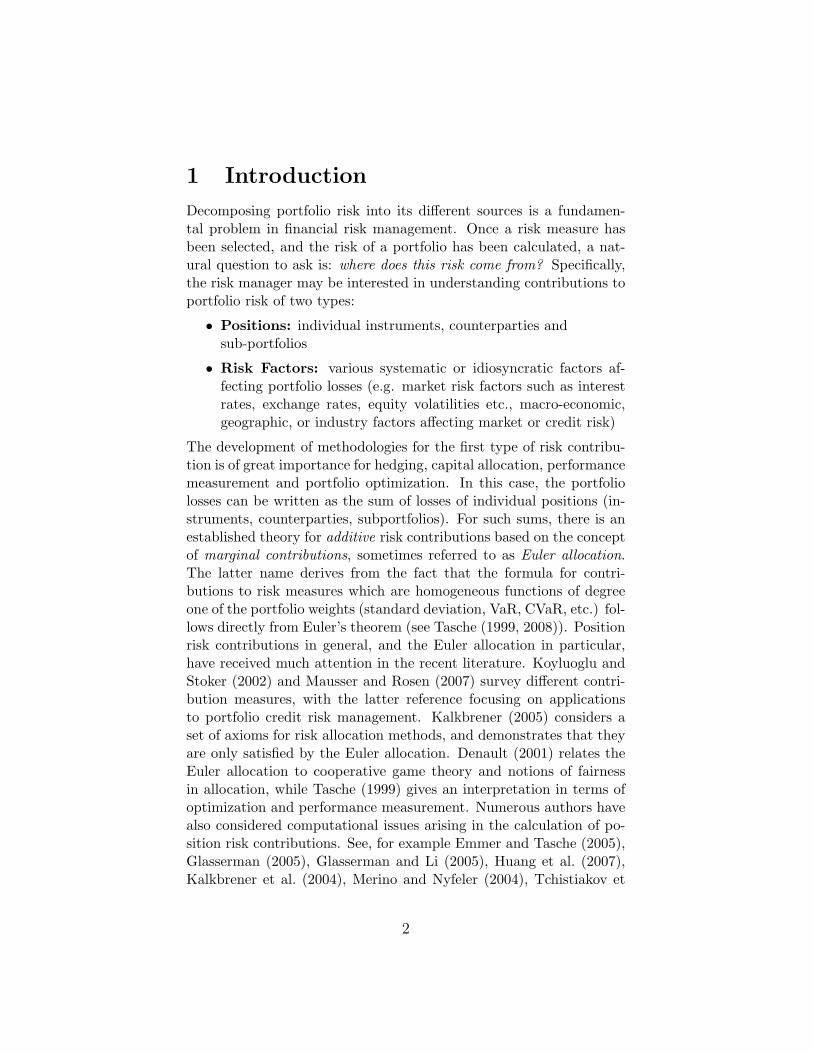
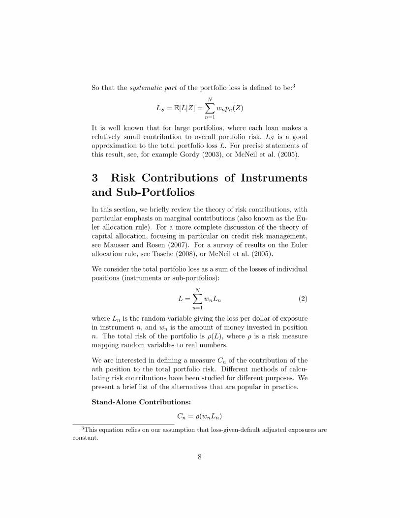
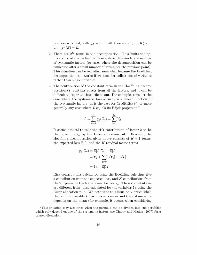
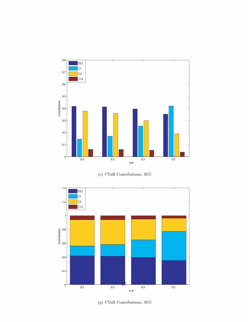
and a lower degree of systematic dependence (i.e. higher idiosyncraticrisk, βB = 0.2), and can be interpreted as the high-yield component ofthe portfolio. We vary the weight wA placed on the investment gradeportion of the portfolio wA = 0.2, 0.3, 0.5, 0.7, with wB = 1 − wA, sothat the weights may be interpreted as the (exposure-weighted) per-centages of wealth invested in each asset class. CVaR contributions fordifferent asset allocations and different confidence levels are given infigures m-v.12 We observe that the contribution of Z1 in isolation (C1)grows quickly in the portfolio weight wA, principally at the expense ofthe contribution C2, and that this effect is more pronounced at higherconfidence levels. The residual contribution of factor co-movementsC12 also tends to decline as the weight wA is increased. This contri-bution is highest when wA is small (wA = 0.2), and the confidencelevel is high (e.g. 99.9%).

5.2 Multi-Factor Example

We now consider as the underlying portfolio the CDXIG index, usingdata from March 31, 2006. One year default probabilities are impliedfrom credit default swap spreads.13 We assume a multi-factor modelwith a single global factor ZG and a set of sector factors ZS repre-senting the systematic risk of industry sectors which is not alreadycaptured by the global factor ZG. The creditworthiness index of aname in sector S is given by:

Y =√ρG · ZG +

√ρS − ρG · ZS +

√1− ρS · ε

where ρG = 0.17 and ρS = 0.23 are parameters that are the same forall instruments. This specification ensures a correlation of ρG for thecreditworthiness indices of two names not in the same sector (inter-sector correlation) and a correlation of ρS for the creditworthiness in-dices of two names in the same sector (intra-sector correlation). Thesevalues are selected to match estimated correlations from Akhavein etal. (2005).

We use a total of seven industrial sectors, consolidated from 25 Fitchsectors. Each name in the index is mapped to one industry sector.

12Again, contributions are calculated using Monte-Carlo without importance sampling,with ten million scenarios.

13Technically then, we are using risk-neutral default probabilities.

25

0.2 0.3 0.5 0.70

0.1

0.2

0.3

0.4

0.5

0.6

0.7

0.8

wA

Con

trib

utio

n

E[L]

C1

C2

C12

(m) CVaR Contributions: 90%

0.2 0.3 0.5 0.70

0.2

0.4

0.6

0.8

1

1.2

1.4

w A

Con

trib

utio

n

E[L]

C1

C2

C12

(n) CVaR Contributions: 90%26

0.2 0.3 0.5 0.70

0.1

0.2

0.3

0.4

0.5

0.6

0.7

0.8

w A

Con

trib

utio

nE[L]

C1

C2

C12

(o) CVaR Contributions: 95%

0.2 0.3 0.5 0.70

0.2

0.4

0.6

0.8

1

1.2

1.4

w A

Con

trib

utio

n

E[L]

C1

C2

C12

(p) CVaR Contributions: 95%

27

0.2 0.3 0.5 0.70

0.1

0.2

0.3

0.4

0.5

0.6

0.7

0.8

w A

Con

trib

utio

n

E[L]

C1

C2

C12

(q) CVaR Contributions: 99%

0.2 0.3 0.5 0.70

0.2

0.4

0.6

0.8

1

1.2

1.4

w A

Con

trib

utio

n

E[L]

C1

C2

C12

(r) CVaR Contributions: 99%

28

0.2 0.3 0.5 0.70

0.1

0.2

0.3

0.4

0.5

0.6

0.7

0.8

w A

Con

trib

utio

n

E[L]

C1

C2

C12

(s) CVaR Contributions: 99.5%

0.2 0.3 0.5 0.70

0.2

0.4

0.6

0.8

1

1.2

1.4

w A

Con

trib

utio

n

E[L]

C1

C2

C12

(t) CVaR Contributions: 99.5%

29

0.2 0.3 0.5 0.70

0.1

0.2

0.3

0.4

0.5

0.6

0.7

0.8

0.9

w A

Con

trib

utio

nE[L]

C1

C2

C12

(u) CVaR Contributions: 99.9%

0.2 0.3 0.5 0.70

0.2

0.4

0.6

0.8

1

1.2

1.4

w A

Con

trib

utio

n

E[L]

C1

C2

C12

(v) CVaR Contributions: 99.9%

30

Aggregate Sector Weight (Exposure) Weight (EL)TECH 20.8% 20.4%

SERVICE 9.6% 9.9%PHARMA 5.6% 3.7%RETAIL 20.0% 27.8%

FINANCE 19.2 % 15.0 %INDUSTRIAL 9.6% 9.8%

ENERGY 15.2% 13.4%

Table 1: CDXIG Index Sector Concentrations

For the details of the mapping, see Rosen and Saunders (2007). Theindustry concentrations for the index are given in Table 1, weightedboth by notional and expected loss. The average one year defaultprobability of the index is 0.19%.

It is easy to see that for this specification of the Gaussian copulamodel, the only nonzero terms in the Hoeffding decomposition corre-spond to the expected loss term, the single factor terms (both globaland sector), and the joint influence terms involving the global factorand one of the sector factors. Percentage CVaR contributions for theseterms for several confidence levels are given in Table 2. Contributionsare calculated using Monte-Carlo simulation with one million scenar-ios. Notice that the global factor dominates the risk contributions.This is not surprising, given that it is the only factor that influencesall of the names. Again, the contribution of the expected loss term ismore significant for lower quantiles, and less significant as one movesfurther in the tail. In this region one also sees a higher contributionfrom the terms giving the joint influence of the global factor and one ofthe sectors. To examine the impact of the parameters on the risk con-tributions calculated by the model, we repeat the calculations withan intra-sector correlation of 70% and an inter-sector correlation of20%. This leads to the results in Table 3. Observe that in this casewe see substantially higher contributions for the industry factors (inparticular TECH and RETAIL).

31

Fac

tor

CVaR

-90%

CVaR

-95%

CVaR

-99%

CVaR

-99.

5%C

VaR

-99.

9%E[L

]19

.13%

13.6

3%7.

19%

5.71

%3.

59%

GLO

BA

L73

.26%

76.9

9%80

.46%

81.1

3%82

.07%

TE

CH

0.78

%0.

67%

0.50

%0.

44%

0.33

%SE

RV

ICE

0.19

%0.

15%

0.09

%0.

07%

0.05

%P

HA

RM

A0.

03%

0.03

%0.

02%

0.01

%0.

00R

ETA

IL1.

35%

1.10

%0.

75%

0.64

%0.

47%

FIN

AN

CE

0.47

%0.

41%

0.31

%0.

26%

0.17

%IN

DU

ST

RIA

L0.

18%

0.16

%0.

11%

0.10

%0.

07%

EN

ER

GY

0.37

%0.

32%

0.21

%0.

19%

0.14

%G

LO

BA

L+

TE

CH

0.95

%1.

52%

2.60

%2.

92%

3.44

%G

LO

BA

L+

SE

RV

ICE

0.24

%0.

35%

0.48

%0.

45%

0.61

%G

LO

BA

L+

PH

AR

MA

0.04

%0.

07%

0.10

%0.

11%

-0.0

2%G

LO

BA

L+

RE

TA

IL1.

53%

2.33

%3.

59%

3.97

%4.

43%

GLO

BA

L+

FIN

AN

CE

0.68

%1.

06%

1.78

%1.

95%

2.18

%G

LO

BA

L+

IND

UST

RIA

L0.

29%

0.42

%0.

64%

0.73

%0.

85%

GLO

BA

L+

EN

ER

GY

0.51

%0.

79%

1.19

%1.

34%

1.62

%

Tab

le2:

CD

XIG

Syst

emat

icFac

tor

CVaR

Con

trib

uti

ons

32

Fac

tor

CVaR

-90%

CVaR

-95%

CVaR

-99%

CVaR

-99.

5%C

VaR

-99.

9%E[L

]11

.63%

6.99

%2.

87%

2.17

%1.

34%

GLO

BA

L32

.76%

27.1

3%19

.27%

17.5

4%16

.15%

TE

CH

8.42

%7.

80%

7.04

%6.

91%

7.95

%SE

RV

ICE

3.09

%2.

44%

1.29

%0.

90%

0.15

%P

HA

RM

A0.

79%

0.57

%0.

15%

0.09

%0.

05%

RE

TA

IL11

.94%

10.8

9%9.

47%

9.20

%9.

11%

FIN

AN

CE

5.69

%5.

06%

4.37

%4.

25%

4.04

%IN

DU

ST

RIA

L3.

06%

2.45

%1.

33%

0.99

%0.

23%

EN

ER

GY

4.65

%4.

08%

3.16

%2.

92%

1.88

%G

LO

BA

L+

TE

CH

3.58

%7.

02%

12.7

5%14

.74%

18.5

2%G

LO

BA

L+

SE

RV

ICE

1.97

%2.

97%

2.88

%2.

27%

0.91

%G

LO

BA

L+

PH

AR

MA

0.73

%0.

92%

0.50

%0.

36%

0.25

%G

LO

BA

L+

RE

TA

IL4.

41%

9.01

%16

.02%

18.0

5%21

.29%

GLO

BA

L+

FIN

AN

CE

2.91

%5.

38%

9.28

%10

.27%

11.6

6%G

LO

BA

L+

IND

UST

RIA

L1.

94%

2.93

%3.

07%

2.55

%1.

15%

GLO

BA

L+

EN

ER

GY

2.42

%4.

36%

6.54

%6.

80%

5.32

%

Tab

le3:

CD

XIG

Syst

emat

icFac

tor

CVaR

Con

trib

uti

ons

33

6 Concluding Remarks

This paper extends the techniques developed for marginal risk contri-butions of portfolio positions (instruments and sub-portfolios) to thecalculation of risk contributions from risk factors, with a focus on ap-plications in portfolio credit risk management. This enables a fullerrisk analysis of any portfolio, where loss contributions can be calcu-lated on both an instrument/sub-portfolio and a risk factor basis togive risk managers’ a better impression of the key drivers of potentialportfolio losses. We employ the Hoeffding decomposition of the lossrandom variable and calculate contributions for each term in this de-composition. We further develop several examples of applications ofthis decomposition technique to factor models of portfolio credit risk.We demonstrate the financial interpretation of the risk contributionsarising from the terms in the Hoeffding decomposition of portfoliolosses. They represent the quadratic “best hedges” involving instru-ments of increasing complexity.

The ideas and examples presented in this paper raise a number of ques-tions that we believe are worthy of consideration in future research.Some of these include:

• From a practical perspective, the development of efficient al-gorithms for the calculation of factor contributions is impor-tant. For example, the application of importance sampling andother techniques used for position contributions (e.g. Glasser-man (2005), Huang et al. (2007), and Merino and Nyfeler (2004))needs to be investigated.

• The development of efficient algorithms for computing the termsof the Hoeffding decomposition, conditional on realizations of thefactor values, is necessary when explicit analytical formulas arenot available. This is crucial to areas such as the risk manage-ment of structured credit portfolios, as well as other non-linearportfolios including equity, fixed-income and FX options.

• From a theoretical perspective, it is important to develop anaxiomatic characterization of factor contribution measures in amanner similar to Kalkbrener et al. (2004).

• Finally, we have related the Hoeffding decomposition to quadratichedges involving instruments of increasing complexity. This tech-nique may be extended to consider best hedges with respect to

34

other risk measures. In particular, it seems natural to considerbest hedges defined by the risk measure ρ whose value for aparticular portfolio we are seeking to allocate. Such hedges areunlikely to be analytically tractable and hence require the devel-opment of efficient numerical algorithms.

35

A Hoeffding Decompositions

This appendix presents a more technical review of Hoeffding decom-positions than that which appears in the main body of the text. Fora fuller discussion, see van der Vaart (1998), sections 11.3-11.4, whichwe follow closely.

Consider a fixed probability space (Ω,F ,Q). Let L be a random vari-able with finite variance, and let Z1, . . . , ZK be independent randomvariables with finite variances. For a given index set A ⊆ 1, . . . ,K,define a closed subspace HA of L2(Q) in the following way. HA con-sists of all square-integrable random variables of the form g(Zi; i ∈ A)for some Borel measurable g (that is, all variables in L2(Q) that aremeasurable with respect to the σ-algebra FA = σ(Zk, k ∈ A)) suchthat additionally:

E[g(Zk, k ∈ A)|Zj , j ∈ B] = 0 (11)

for every B such that |B| < |A|. Then we have the direct sum:

L2(Ω,FA,Q) =⊕B⊆A

HB (12)

Denoting by PB the projection onto HB, we then obtain the (orthog-onal) decomposition:

E[L|FA] = E[L|Zk, k ∈ A] =∑B⊆A

PBL (13)

The projections PA can be evaluated more explicitly (for a proof, seevan der Vaart (1998)):

PAL =∑B⊆A

(−1)|A|−|B| · E[L|Zk, k ∈ B] = gA(Zk; k ∈ A) (14)

In particular, if L = g(Z1, . . . , ZK), then by taking A to be the fullindex set, A = 1, . . . ,K in (12) we obtain:

L =∑

B⊆1,...,K

gB(Zk; k ∈ B)

=∑

B⊆1,...,K

∑B′⊆B

(−1)|B|−|B′| · E[L|Zk, k ∈ B′] (15)

this is called the Hoeffding decomposition of the random variable L.

36