Risk, External Adjustment and Capital Flows

Martin D. D. Evans

Department of Economics

Georgetown University

⇤

Second Draft

December 30, 2013

This paper studies the process of external adjustment. I develop an open economy model with endowment

and preference shocks that can account for the empirical behavior of real exchange rates, interest rates and

consumption in the U.S. and Europe. The model includes cross border holdings of bonds and equity,

and financial frictions that impede international risk-sharing. I find that external adjustment following

endowment shocks predominantly takes place via trade flows, consistent with the intertemporal approach to

the current account. In contrast, preference shocks that change investors’ risk aversion induce adjustment

via the trade and valuation channels; where the latter includes the effects of unexpected capital gains and

loss on existing cross border holdings and changes in the expected future return differentials between foreign

assets and liabilities. The model estimates imply that the valuation channel of external adjustment is more

important for the U.S. than the trade channel. Consistent with this implication, I show that forecasts of

future return differentials contributed most to the volatility of the U.S. net foreign asset position in the post

Bretton-Woods era.

Keywords: International Capital Flows, External Adjustment, Open-Economy Macro Models, Habits, In-

complete Markets, Collateral Constraints.

JEL Codes: F3; F4; G1.

*This paper was prepared for the International Seminar on Macroeconomics held at the Bank of Italy in June

2013. I thank the Guest Editor, Gita Gopinath; the anonymous referees; the discussants, Jeffrey Frankel and Robert

Kollmann; and the other seminar participants for many useful comments. Any remaining errors are my own. Email:

evansmdd@gmail.com.

Introduction

A central challenge in international macroeconomics is to understand how unexpected changes in economic

conditions in one country are transmitted internationally via international trade and financial markets. In

principle, the process of external adjustment can take place via changes in consumption and investment

decisions that generate international trade flows, via unexpected variations in asset prices, and through

changes in risk premia that produce portfolio re-allocations driving international capital flows. In practice,

our understanding of the process is very incomplete. What factors determine the importance of these different

adjustment channels? Does greater integration of world financial markets facilitate adjustment or simply

increase an economy’s susceptibility to adverse foreign shocks? Are the persistent and large imbalances in

current accounts and net foreign asset positions we observe across the world consistent with a well-functioning

adjustment process or are they a symptom of a fragile international financial system?

Unfortunately, standard open economy macro models give limited guidance on these questions. In canon-

ical models where all international borrowing and lending take place via a single risk free bond, external

adjustment takes place entirely via the current account reflecting revisions in forward-looking consumption

and investment decisions. This perspective on adjustment, referred to as the intertemporal approach to the

current account (see, e.g., Obstfeld and Rogoff, 1995), ignores the fact that there are large cross border

holdings of many financial assets in different currencies, not just holdings of a single risk free bond. As

such, it is silent on the possible adjustment roles played by unexpected capital gains and losses on existing

holdings and expected capital gains and losses on future holdings that compensate investors for risk. These

valuation effects may be empirically important. Gourinchas and Rey (2013) observe that changes in the net

foreign asset positions of many counties appear to be increasingly influenced by capital gains and losses. Are

these gains and losses unanticipated; or do they represent, in part, compensation for risk? More generally,

are these financial effects benign, reflecting efficient risk sharing, or do they impede adjustment? The aim

of this paper is to make progress on these questions. For this purpose I develop a new open economy model

that allows for multiple channels of external adjustment and use it to assess their empirical importance.

The model is built around a standard core. There are two countries, each populated by a continuum

of infinitely-lived households with preferences exhibiting home bias defined over the consumption of two

perishable traded goods. Households have access to a wide array of financial assets: domestic equity and risk

free bonds as well as foreign equity and bonds. Their optimal portfolio decisions are the driver of international

capital flows in bonds and equity. On the production side I assume that the world supply of each traded good

follows an exogenous endowment process and that there are no impediments to international goods trade. I

add three key elements to this simple structure: collateral constraints that limit international borrowing, a

portfolio friction that limits the flexibility households have in re-allocating their wealth among foreign bonds

and equity, and habits in households’ preferences (adapted from Campbell and Cochrane, 1999). The first

two elements make markets incomplete so households’ portfolio decisions affect equilibrium consumption,

savings and international trade flows. The third element allows me to compare external adjustment following

temporary output/endowment shocks with the adjustment following heteroskedastic preference shocks that

change households’ risk aversion. The financial and macro effects of these risk shocks are quite different from

1

output/endowment shocks and play a central role in my analysis.

The model identifies two distinct adjustment processes; one triggered by output shocks and one triggered

by risk shocks. Adjustment following output shocks occurs via international trade and unexpected capital

gains. For example, a shock that temporarily raises the output of the domestic good induces a deterioration

in the terms of trade (i.e. a fall in the relative price of domestic to foreign traded goods), and a rise

(fall) in domestic (foreign) aggregate consumption. These adjustments ensure goods market clearing in the

presence of home consumption bias. They also imply a jump depreciation in the real exchange rate followed

by an expected future appreciation, and a fall in the domestic real interest rate relative to the foreign

rate as households smooth consumption intertemporally - consistent with uncovered interest parity (UIP).

The shock also produces higher domestic dividends together with unexpected capital gains on domestic

equity and foreign asset holdings that finance domestic trade deficits until it dissipates. In sum, output

shocks produce adjustments via international trade and unexpected gains/loses on existing net foreign asset

positions. Quantitatively, most adjustment takes place via trade, referred to as “the trade channel” by

Gourinchas and Rey (2007).

Adjustments triggered by risk shocks follow a different pattern because they change the risk premia

embedded in expected future returns on domestic and foreign assets. For example, a shock that temporarily

increases the risk aversion of domestic households induces an immediate appreciation in the real exchange

rate. This improves international risk sharing (i.e., it reduces the difference between marginal utility across

countries) but it also produces unexpected capital losses on domestic equity and foreign asset positions when

domestic marginal utility is high. Households view these adverse valuation effects as more likely in the

future because the current risk shock increases the likelihood of future shocks (via heteroskedasticity), so in

equilibrium the risk premia on domestic equity and foreign assets (equity and bonds) rise to compensate.

As a result, the risk shock produces an initial unexpected capital loss on the domestic net foreign asset

position and higher expected future returns on foreign assets relative to liabilities until its effects dissipate.

Beyond these external valuation adjustments, the risk shock increases domestic precautionary saving which

lowers the real interest rate. As a consequence, there is a fall in real interest differential and a rise in the

foreign exchange risk premium (the risk premium embedded in the expected excess return on foreign bonds)

that together match the expected real depreciation rate following the shock. Unlike the pattern following

output shocks, these adjustments are inconsistent with UIP. The risk shock also produces a trade surplus

because the appreciation in the exchange rate improves the terms of trade. However, external adjustment via

trade is quantitatively much less important than through the capital gains/loses and risk premia variations,

collectively referred to as “the valuation channel” by Gourinchas and Rey (2007).

Clearly, these adjustment processes are quite different: temporary output shocks primarily trigger ad-

justment via the trade channel, while risk shocks mainly produce adjustment via the valuation channel. The

contributions of these channels to actual adjustment thus depends on the relative importance of (temporary)

output and risk shocks as drivers of international business cycles. To address this issue, I estimate the

parameters of endowment and habit processes (driven by output and risk shocks respectively) so that the

second moments for equilibrium real depreciation rates, interest rates and consumption growth rates in the

model match their counterparts in quarterly U.S. and E.U. data. This estimation procedure reveals that

2

risk shocks are a much more important driver of exchange rate, interest rate and consumption dynamics in

U.S./E.U. data than temporary output shocks. The key reason for this is that risk shocks produce a strong

negative correlation between future depreciation rates and the current real interest differential via variations

in the foreign exchange risk premium, whereas endowment shocks produce a positive correlation consistent

with UIP. In U.S./E.U. data, future depreciation rates are strongly negatively correlated the current interest

differential, so the incidence of risk shocks needs to be high for the model to replicate this feature of the

data. The high incidence of risk shocks also allows the model to match the empirical volatilities of real

depreciation rates, interest differentials and consumption growth rates.

My estimation results imply that valuation effects (driven by risk shocks) should play an important role

in the U.S. external adjustment process. To investigate this implication of the model, I estimate the role

of valuation effects in the U.S. process. Gourinchas and Rey (2007) first studied the empirical importance

of the trade and valuation channels of external adjustment in the U.S. using an approximation that linked

a country’s external position to forecasts of future net export growth (identifying the trade channel) and

forecast of future returns on foreign assets and liabilities (identifying the valuation channel). They found

that the valuation channel accounted for approximately 30 percent of the cyclical variations in U.S. external

position between 1952 and 2004. I use a similar approximation to estimate the contribution of forecast

revisions for net export growth and returns to the variance of the U.S. net foreign asset position between

1973 and 2007. My estimates indicate that the valuation channel was more important than the trade channel

during this period, contributing between 60 and 88 percent of variance. When I perform the same calculations

with data from the estimated model, I find that the valuation channel accounts for 86 percent of the variance

in the net foreign asset position.

Finally, I examine the implications of the estimated model for the behavior of international capital

flows. Since households can hold domestic and foreign bonds and equity, the model allows for complex

patterns of bond and equity inflows and outflows as part of the external adjustment process. Once again,

these patterns depend on the shock triggering adjustment. Output shocks produce very small capital flows

because they have negligible effects on households portfolio decisions. The international trade flows induced

by the shocks are finance by capital gains/losses on existing positions and changes in dividends. In contrast,

risk shocks produce debt and equity flows as households re-allocate their portfolios in the face of changing

risk premia and risk aversion. It is here that the effects of financial frictions in the model appear most

clearly. Intuitively, the portfolio friction stops the equilibrium risk premia on foreign equity and bonds from

adjusting to a point where all households are willing to maintain their pre-existing holdings, so flows arise

as household establish new optimal positions. These flows are also affected by the presence of collateral

constraints. Unexpected capital losses that push households closer to the point where the constraint binds

induce portfolio re-allocations that amplify the capital flows produced by the portfolio friction. According

to the model estimates, the presence of collateral constraints doubles the size of the debt and equity capital

flows induced by risk shocks.

The remainder of the paper is divided into six sections. The model I develop draws on several lines of

research from the asset-pricing and open-economy macro literatures. Section 1 discusses this research and

explains where I extend existing work. Section 2 presents the model. Section 3 explains how I solve and

3

calibrate the model to match the U.S. and E.U. data. In Section 4 I identify the elements that contribute

to the external adjustment process. Section 5 contains my quantitative analysis of the model, including my

empirical examination of the U.S. external adjustment process. Section 6 concludes. Information concerning

the data used in my empirical analysis, the solution method and other mathematical details can be found in

the Web Appendix.

1 Related Literature

My analysis is related to three main areas of research: The first studies the asset-pricing implications of

non-standard preferences, the second examines portfolio choice in open economy general equilibrium models,

and the third focuses on the process of international external adjustment.

This paper adds to a large literature that uses habit formation to explain asset prices in closed and open

economies (see, e.g., Sundaresan, 1989, Abel 1990, Constantinides 1990, Detemple and Zapatero 1991, Ferson

and Constantinides 1991, Heaton 1995, Jermann 1998, Boldrin, Christiano, and Fisher 2001, Chan and Kogan

2002, Menzly, Santos, and Veronesi 2004, Santos and Veronesi 2010 and Buraschi and Jiltsov 2007). The

model I develop adapts the Campbell and Cochrane (1999) habit specification to an open-economy setting.

In their model habits are a function of past consumption shocks which are completely determined by an

exogenous endowment process. As in Bekaert, Engstrom, and Xing (2009), I allow habits to depend on

domestic consumption and exogenous preference shocks. These shocks have the natural interpretation of

risk shocks because they change the local curvature of the households’ utility. They are correlated with

equilibrium consumption via variations in the terms of trade so that habits remain tightly linked to current

and past consumption, as in Campbell and Cochrane (hereafter C&C).

In the C&C model consumption shocks can have differing effects on the marginal utility of investors

(depending the proximity of current consumption to the level of habit) producing variations in the price of

risk. Several papers in the international asset-pricing literature exploit this feature. Verdelhan (2010) uses the

C&C habit specification to account for deviations from UIP in a two-country model with complete markets.1

In his model shocks to domestic consumption produce pro-cyclical movements in the real interest rates and

counter-cyclical variations in the foreign exchange risk premia. Moore and Roche (2010) and Heyerdahl-

Larsen (2012) also use models with habits and complete markets to account for UIP deviations, but here

habits are relate to the consumption of individual goods (so called deep-habits). The model I present extends

this line of research in two directions: First, I estimate parameters of the model so that it replicates the

UIP deviations in U.S. and E.U. data in an equilibrium with incomplete risk-sharing and financial frictions.

Second, I specify households’ preferences over multiple traded goods to allow for consumption home bias,

international trade and realistic co-movements between real exchange rates and the terms of trade (see,

e.g., Engel, 1999).2 These extensions narrow the gap between international asset-pricing and open economy1Under conventional rational expectations assumptions, UIP implies that the slope coefficient from a regression of future

exchange rate changes on the current differential between domestic and foreign risk-free rates should equal one. Instead, a verylarge literature finds estimates less than one and often negative; see, Lewis (1995) and Engel (1996, 2013) for surveys. Theliterature refers to these findings as deviations from UIP, the UIP puzzle or the forward premium anomaly.

2In contrast, Verdelhan (2010) assumes that households only consume domestically produced goods. This extreme form ofhome bias allows him to circumvent the problems induced by variations in the terms of trade but at the cost of eliminating

4

macro literatures (see, e.g., Engel, 2013 and Lewis, 2011).

The model I develop falls into the class of dynamic general equilibrium models with portfolio choice.

Papers by Coeurdacier and Gourinchas (2008), Engel and Matsumoto (2009), Coeurdacier, Kollmann, and

Martin (2010), Hnatkovska (2010), Devereux and Sutherland (2011), Coeurdacier and Rey (2012) and others

use these models to examine the reasons for home bias in equity portfolio holdings. This literature considers

home bias arising from exchange-rate risk and non-tradable income risk, primarily in a complete markets

setting. In contrast, home equity bias arises in my model because financial frictions stop the equilibrium risk

premia from providing sufficient compensation to households for the poor exchange-rate hedging properties

of foreign equity. These frictions also impede international risk sharing. In this respect the my analysis

adds to a growing literature studying open economy models with portfolio choice and incomplete markets

(see, e.g., Evans and Hnatkovska, 2013 and 2007, Hnatkovska, 2010, Devereux and Sutherland, 2011, and

Tille and van Wincoop, 2010). One distinctive feature of my analysis relative to this literature concerns

the solution method used to compute the equilibrium of the model. Both Devereux and Sutherland (2011)

and Tille and van Wincoop (2010) use a method that approximates the financial side of the model in the

neighborhood of deterministic steady state where differences between expected returns on risky assets are

very small.3 This paper adapts the solution method developed by Evans and Hnatkovska (2012) to allow for

the presence of collateral constraints. Importantly, it approximates the equilibrium of the model around a

stochastic steady state where there are significant differences in the risk characteristics of different financial

assets (e.g., domestic vs. foreign equity). These differences are reflected in the steady state risk premia, and

in how the premia react to risk shocks - a central focus of my analysis.

My analysis also relates to research on the joint determination of capital flows and equity returns. Repre-

sentative papers in this area include Bohn and Tesar (1996), Froot and Teo (2004) and Froot, O’Connell, and

Seasholes (2001). Hau and Rey (2006, 2004) extend the analysis of the equity return-capital flow interaction

to include the real exchange rate. Evans and Hnatkovska (2013), Devereux and Sutherland (2011), Tille and

van Wincoop (2010) and Coeurdacier, Kollmann, and Martin (2010) all model capital flows as the result of

optimal portfolio reallocations in a similar manner to this paper. Noteworthy aspects of my analysis relative

to these papers include: (i) the contrast between the effects of risk shocks on equity returns and capital flows

and the effects of output shocks; and (ii) the role of collateral constraints.

Finally, the paper adds to a growing empirical and theoretical literature on international external adjust-

ment. My empirical analysis of the U.S. external position is most closely related to the work of Gourinchas

and Rey (2007) (noted above), but I examine variations in a measure of the total external position rather

international trade. Bansal and Shaliastovich (2010) and Colacito and Croce (2011) also assume an extreme form of home biasto avoid a similar problem in their adaption of the long-run risk framework proposed by Bansal and Yaron (2004). In Mooreand Roche (2010) households consume a basket comprising a single traded and nontraded good so variations in the terms oftrade are absent. This is also true in the Appendix of Verdelhan (2010) which considers a model variant where householdsconsume a single trade good subject to trading costs. Stathopoulos (2012) also studies a two-country external habit modelwhere households’ preferences are defined over multiple traded goods. His focus is on the co-movements in consumption growthand real exchange rates rather than the forward premium anomaly. And, again, he studies a complete markets equilibriumwithout financial frictions.

3Technically speaking, the approximate solution to the model is computed by a perturbation method where the standarddeviation of the exogenous shocks is one of the perturbation variables. Approximations to the expected returns on risky assetsderived from this approach differ from zero to second-order (i.e. they depend on the variance of the shocks), so they are verysimilar across assets near the approximation point used to solve the model.

5

than the cyclical measure they study. This difference in focus accounts for the larger estimated contribution

of the valuation channel I estimate. Corsetti and Konstantinou (2012) also study the cyclical dynamics of

the U.S. external position. They find that transitory shocks drive changes in the net foreign asset position

while variations in aggregate consumption and gross positions are dominated by permanent shocks. In my

model, risk shocks are the dominant source of transitory shocks that drive the net foreign asset position

while permanent endowment shocks (common to all goods) change gross asset positions. On the theoretical

side, Pavlova and Rigobon (2008), Tille and van Wincoop (2010) and Devereux and Sutherland (2011) all

study external adjustment in open economy models with incomplete markets. In these models valuation

adjustment takes place via unexpected capital gains and losses rather than through changes in the expected

return differentials between foreign assets and liabilities.4

2 The Model

The model comprises two symmetric countries, which I refer to as the U.S. and Europe. Each country is

populated by infinitely-lived households with preferences defined over the consumption of two perishable

traded goods. For simplicity, there are no nontraded goods or impediments to trade in goods between the

two countries. I also assume that the world supply of each traded good follows an exogenous endowment

process, one located in each country.5 The model includes three key features beyond this simple structure:

habits in household preferences, a collateral constrain that limits international borrowing, and a restriction

that limits portfolio reallocations among foreign assets.

2.1 Household Preferences

Each country is populated by a continuum of identical households distributed on the interval [0,1]. House-

holds’ preferences are defined over a basket of traded consumption goods. In particular, the expected utility

of a representative U.S. household i 2 [0, 1] in period t is given by

Ui,t

= Et

1X

j=0

�jU(Ci,t+j

, Ht+j

), with U(Ci,t

, Ht

) =

1

1��

{(Ci,t

�Ht

)

1�� � 1}, (1)

where 1 > � > 0, � > 0 and Et

denotes expectations conditioned on period-t information, which is common

to all households. Each household’s sub-utility U(Ci,t

, Ht

) depends on current consumption, Ci,t

, and the

subsistence level of consumption, or habit level, Ht

. This habit level is treated as exogenous by individual

U.S. households but varies with aggregate U.S. consumption, Ct

.6 Specifically, let St

= (Ct

�Ht

)/Ct

denote4In Pavlova and Rigobon (2008) households have log preferences so there is no intertemporal hedging and risk premia are

constant. Shocks produce negligible changes in expected return differentials between foreign assets and liabilities in Devereuxand Sutherland (2011) and Tille and van Wincoop (2010) for the reasons discussed above.

5This assumption rules out the possibility that domestic production could be impaired by the effects of capital outflowson domestic credit markets, as in the literature on sudden stops. Clearly, this is a concern in economies where the domesticbanking system is heavily dependent on foreign funding and domestic firms have limited access to world capital markets. Myfocus in this paper is on large economies where these issues are much less of a concern. I leave the task of extending the modelto include production and domestic banking for future work.

6In this specification the level of habit is determined externally by the consumption decisions of all U.S. households. Alter-natively, the level of habit could be determined internally by the consumption decisions of individual households. C&C find

6

the aggregate surplus consumption ratio. Following C&C, I assume that the log surplus ratio st

= ln(St

)

follows a heteroskedastic AR(1) process

st+1

= (1� �)s+ �st

+ !(st

)vt+1

, (2)

where 1 > � > 0 and s is the steady state value of st

. (Hereafter I use lowercase letters to denote the natural

log of their uppercase counterpart.) The i.i.d. mean-zero, unit variance vt

shocks affect the surplus ratio

via a non-negative sensitivity function !(st

), which I discuss below. Notice that the U.S. habit level is given

by Ht

= [1 � exp(st

)]Ct

so negative vt

shocks raise habit relative to current aggregate consumption, but

they cannot push habit above current consumption. The surplus ratio also determines the local curvature

of households’ utility functions. For a representative household �Ci,t

Uc

(Ci,t

, Ht

)/Ucc

(Ci,t

, Ht

) = �/St

, so

their risk aversion tends toward infinity as the surplus ratio goes to zero.

The U.S. consumption basket comprises U.S. and E.U. traded goods:

Ci,t

= C(Cusi,t

, Ceui,t

) =

⇣

⌘1✓Cus

i,t

✓�1✓

+ (1� ⌘)1✓ Ceu

i,t

✓�1✓

⌘

✓✓�1

, (3)

where Cusi,t

and Ceui,t

identify the consumption of U.S. and E.U. goods by U.S. household i. The parameter

⌘ 2 (0, 1) governs the desired share of each good in the basket and ✓ is the elasticity of substitution between

goods. I follow standard practice in the literature and focus on the case where ⌘ > 1/2, so that households’

preferences exhibit consumption home-bias.

E.U. household i 2 [0, 1] has analogous preferences:

bUi,t

= Et

1X

j=0

�jU( ˆCi,t+j

, ˆHt+j

), (4)

where the E.U. consumption basket is

ˆCi,t

= C( ˆCeui,t

, ˆCusi,t

, ) =⇣

⌘1✓ ˆCeu

i,t

✓�1✓

+ (1� ⌘)1✓ ˆCus

i,t

✓�1✓

⌘

✓✓�1

. (5)

The external E.U. habit level ˆHt

= [1� exp(st

)]

ˆCt

depends on aggregate E.U. consumption, ˆCt

, and the log

surplus ratio, st

= ln

ˆSt

, which follows

st+1

= (1� �)s+ �st

+ !(st

)vt+1

, (6)

where vt+1

are i.i.d. mean-zero, unit variance shocks. As above, the surplus ratio ˆSt

determines the local

curvature of E.U. household utility: � ˆCi,t

Uc

(

ˆCi,t

, ˆHt

)/Ucc

(

ˆCi,t

, ˆHt

) = �/ ˆSt

.

In the C&C model shocks to the log surplus ratio are perfectly correlated with unexpected changes in

aggregate consumption. In their closed economy equilibrium consumption is determined by an endowment

process so unexpected consumption depends on the exogenous endowment shock. This specification also

that most asset-pricing implications of their model are robust to the presence of internal rather than external habits. Sincemodels with internal habits are inherently more complex, I utilize the external habit specification here.

7

implies that the level of external habit is a nonlinear function of current and past aggregate consumption.

Here, in contrast, each country’s aggregate consumption comprises a basket of traded goods so shocks

affecting the endowments of either good and/or relative prices contribute to unexpected consumption in

both countries. Thus, in this setting the C&C specification would produce a cross-country correlation

between shocks to the log surplus ratios that greatly complicates the analysis of how changes in risk-aversion

are transmitted internationally. To facilitate this analysis, I assume instead that shocks to the log surplus

processes in (2) and (6) are independent and exogenous. They thus have the natural interpretation as risk

shocks because they change the local curvature of households’ utility. This specification enables us to study

how changes in risk aversion originating in one country are transmitted internationally by tracing their effects

on equilibrium asset prices and capital flows.

My specification for the st

and st

processes has two other noteworthy implications. First, it does not rule

out a correlation between consumption growth and the log surplus ratio in each country. On the contrary, risk

shocks affect consumption growth because they alter the real exchange rate and the terms of trade, which in

turn induce households to adjust the composition of their consumption baskets. Thus, consumption growth

is correlated with the log surplus ratios, but the correlation is imperfect and is determined as part of the

model’s equilibrium. This feature of the model is consistent with the results in Bekaert, Engstrom, and

Xing (2009). They find evidence in U.S. data of an imperfect correlation between the log surplus ratio and

consumption growth in a model that adds exogenous shocks to the C&C specification.

The second implication concerns the dynamics of habits. By definition the level of U.S. habit is given

by Ht

= [1 � exp(st

)]Ct

, so domestic risk shocks can in principle affect the level of habit independently of

their effect on aggregate consumption (i.e., via their impact on st

). This is not an important effect in the

calibrated equilibrium of the model. I show below that almost all the variations in the level of habit are

related to current and past innovations in domestic consumption.

The processes for the log surplus ratios in (2) and (6) also contain a sensitivity function that governs the

reaction of the ratios to risk shocks. I assume that the function is decreasing in the log surplus:

!(s) =

8

<

:

p

!(smax

� s) s smax

0 s > smax

,

where ! is a positive parameter. In the continuous time limit, st

and st

never exceed the upper bound of

smax

, so there is a corresponding lower limit on households’ risk-aversion. The sensitivity function in the

C&C specification is also decreasing in the log surplus ratio but is parameterized to keep risk free interest

rates constant. The specification here allows for variations in the risk free rates depending on the values for w

and smax

. I estimate these parameters from data on real exchange rates, real interest rates and consumption

below.

Prices and Exchange Rates

The model contains two international relative prices: the terms of trade and the real exchange rate. These

prices are linked through the consumption price indices in each country. Let P ust

and P eut

denote the prices

8

of the U.S. and E.U. goods in dollars, while ˆP ust

and ˆP eut

denote their prices in euros, respectively. The U.S.

and E.U. price indices corresponding to the consumption baskets in (3) and (5) are

Pt

=

✓

⌘(P ust

)

1�✓

+ (1� ⌘) (P eut

)

1�✓

◆

11�✓

and ˆPt

=

✓

⌘( ˆP eut

)

1�✓

+ (1� ⌘) ( ˆP ust

)

1�✓

◆

11�✓

.

The real exchange rate is defined as the relative price of the E.U. consumption basket in terms of the U.S.

basket, Et

= St

ˆPt

/Pt

, where St

denotes the dollar price of euros. There are no impediments to international

trade between the U.S. and the E.U. so the law of one price applies to both the U.S. and E.U. goods: i.e.,

P ust

= St

ˆP ust

and P eut

= St

ˆP eut

. Combining these expressions with the definitions of the real exchange rate

and the price indices gives

Et

=

✓

⌘Tt

1�✓

+ (1� ⌘)

⌘ + (1� ⌘) Tt

1�✓

◆

11�✓

, (7)

where Tt

denotes the U.S. terms of trade, defined as the relative price of imports in terms of exports, P eut

/P ust

.

When there is home bias in consumption (⌘ > 1/2), a deterioration in the U.S. terms of trade (i.e. a rise in

Tt

) is associated with a real depreciation of the dollar (i.e. a rise in Et

).

Equation (7) makes clear that the model attributes all variations in real exchange rates to changes in

the relative prices of traded goods via the terms of trade. This feature of the model is broadly consistent

with existing empirical evidence on the source of real exchange rate variations. For example, Engel (1999)

finds that little of the variation in real depreciations rates over horizons of five years or less originate from

differences between the relative prices of traded and nontraded goods across countries. The omission of

non-traded goods from the model doesn’t significantly impair its ability to replicate the short- and medium-

term dynamics of real exchange rates. Equation (7) also implies that the real depreciation rate is strongly

correlated with changes in the terms of trade when there is home bias in consumption. This implication is

also consistent with the data. Real depreciation rates are very strongly correlated with changes in terms of

trade over short horizons (see, e.g., Evans, 2011).

Assets and Goods Markets

There are four financial markets: a market for U.S. equities, E.U. equities, U.S. bonds and E.U. bonds. U.S.

equity represents a claim on the stream of U.S. good endowments. In particular, at the start of period t,

the holder of one share of U.S. equity receives a dividend of Dt

= (P ust

/Pt

)Yt

, measured in terms of the

U.S. consumption basket, where Yt

is the endowment of the U.S. good. The ex-dividend price of U.S. equity

in period t is Qt

, again measured in terms of U.S. consumption. A share of E.U. equity pays a period-t

dividend of ˆDt

= (

ˆP eut

/ ˆPt

)

ˆYt

and has an ex-dividend price of ˆQt

, where ˆYt

is the period-t endowment of the

E.U. good. Notice that ˆQt

and ˆDt

are measured relative to the E.U. consumption basket. The gross real

returns on U.S. and E.U equity are given by

Reqt+1

= (Qt+1

+Dt+1

)/Qt

and ˆReqt+1

= (

ˆQt+1

+

ˆDt+1

)/ ˆQt

.

9

Households can also hold one-period real U.S. and E.U. bonds. The gross return on holding U.S. bonds

between periods t and t + 1 is Rt

, measured in terms of U.S. consumption; the analogous return on E.U.

bonds is ˆRt

, measured in terms of E.U. consumption.

Households have access to both domestic and foreign bond and equity markets subject to two financial

frictions (discussed below). Let Busi,t

, Beui,t

, Ausi,t

and Aeui,t

respectively denote U.S. household i0s holdings of

U.S. and E.U. bonds, and shares of U.S. and E.U. equity in period t. The budget constraint facing the

household is

Et

ˆQt

Aeui,t

+ Et

Beui,t

+Qt

Ausi,t

+Busi,t

+ Ci,t

=

Rt�1

Busi,t�1

+Ausi,t�1

(Qt

+Dt

) + Et

ˆRt�1

Beui,t�1

+ Et

Aeui,t�1

(

ˆQt

+

ˆDt

). (8)

Notice that the first two terms on the left-hand-side represent the value of U.S. foreign asset holdings in

period t. The budget constraint facing E.U. household i is

Qt

ˆAusi,t

/Et

+

ˆBusi,t

/Et

+

ˆBeui,t

+

ˆQt

ˆAeui,t

+

ˆCi,t

=

ˆAeui,t�1

(

ˆQt

+

ˆDt

) +

ˆRt�1

ˆBeui,t�1

+Rt�1

ˆBusi,t�1

/Et

+

ˆAusi,t�1

(Qt

+Dt

)/Et

, (9)

where ˆBusi,t

, ˆBeui,t

, ˆAusi,t

and ˆAeui,t

respectively denote the number of U.S. bonds, E.U. bonds and the number of

shares of U.S. and E.U. equity held by E.U. household i in period t.

The market clearing conditions are straightforward. Both U.S. and E.U bonds are in zero net supply so

the bond market clearing conditions are

0 =

ˆ1

0

Busi,t

di+

ˆ1

0

ˆBusi,t

di and 0 =

ˆ1

0

Beui,t

di+

ˆ1

0

ˆBeui,t

di. (10)

The supplies of the U.S. and E.U. equities are normalized to one, so market clearing requires that

1 =

ˆ1

0

Ausi,t

di+

ˆ1

0

ˆAusi,t

di and 1 =

ˆ1

0

Aeui,t

di+

ˆ1

0

ˆAeui,t

di. (11)

Market clearing in the goods markets requires that aggregate demand from U.S. and E.U. households matches

the world endowment of each traded good:

Yt

=

ˆ1

0

Cusi,t

di+

ˆ1

0

ˆCusi,t

di and ˆYt

=

ˆ1

0

Ceui,t

di+

ˆ1

0

ˆCeui,t

di. (12)

Endowments of the two traded goods are driven by exogenous non-stationary processes. Specifically, I

assume that the log endowments yt

= lnYt

and yt

= ln

ˆYt

follow:

yt

= zt

+ zt

and yt

= zt

+ zt

, with (13a)

zt

= zt�1

+ g + ut

, zt

= ⇢zt�1

+ et

and zt

= ⇢zt�1

+ et

. (13b)

10

Here zt

identifies the stochastic trend (unit root process), while zt

and zt

denote the cyclical components

that follow AR(1) processes with 1 > ⇢ > 0. The three endowment shocks, ut

, et

and et

are mutually

uncorrelated mean-zero random variables, with variances �2

u

, �2

e

and �2

e

, respectively. In the absence of any

shocks, both endowments grow at rate g.

Financial Frictions and Household Decisions

Households face two financial frictions when making their optimal consumption and portfolio decisions. The

first limits their ability to reallocate their foreign asset holdings between bonds and equities. The second

friction takes the form of a collateral constraint that prevents rolling over international debt through the use

of Ponzi schemes.

I assume that households cannot hold foreign equity and bonds directly. Rather, they can hold them

indirectly in a foreign asset mutual fund with fixed proportions. Specifically let FAi,t

= Et

ˆQt

Aeui,t

+ Et

Beui,t

denote the value of the foreign mutual fund held by U.S. household i in period t. The portfolio weights for

equity and bonds in the fund are fixed at } and 1 � }, so that the value of E.U. equity and bond holdings

held indirectly by U.S. household i are

Et

ˆQt

Aeui,t

= }FAi,t

and Et

Beui,t

= (1� })FAi,t

. (14)

Similarly, E.U. households hold U.S. bonds and equities indirectly as part of a their foreign mutual fund,dFA

i,t

= Qt

ˆAusi,t

/Et

+

ˆBusi,t

/Et

, such that

Qt

ˆAusi,t

/Et

= }dFAi,t

and ˆBusi,t

/Et

= (1� })dFAi,t

. (15)

The return on U.S. and E.U foreign asset mutual funds are given by

Rfat+1

= (Et+1

/Et

)(} ˆReqt+1

+ (1� }) ˆRt

) and ˆRfat+1

= (Et

/Et+1

)(}Reqt+1

+ (1� })Rt

).

These assumptions limit households’ ability to change the composition of their foreign asset portfolios

but not the value of foreign assets in their total wealth. Obviously, they are not an accurate description of

the actual re-allocation costs households face, but they can be interpreted as arising from the presence of

fixed transaction costs.7 Suppose, for example, that each period households could choose from a continuum

of foreign asset mutual funds, each characterized by a different value for }. Further, assume that establishing

an account with a fund incurs a fixed cost, while changing the amount invested in an existing account does

not. In the steady state all households would establish an account in the fund with the value for }, say

}⇤, that maximized expected utility. Away from the steady state, they would compare the utility from

moving to a new fund net of the fixed cost with the utility of keeping the }⇤ fund. If the fixed costs were

sufficiently large, households would find it optimal to vary the amount of wealth invested in the }⇤ fund,7An alternative would be to assume that households could hold foreign assets directly and incur a transaction cost whenever

they change their holdings (see e.g., Meier, 2013). This approach would also give households’ more flexibility in reallocatingtheir wealth among domestic than foreign assets, but the explicit introduction of transaction costs would add significantly toan already complex model.

11

so the assumption above would hold with } = }⇤. This fixed cost interpretation is broadly consistent with

U.S. data. In Section 3.3 I show that the value for }⇤ implied by the model is close the value for } implied

by the average equity-to-debt ratio in U.S. foreign asset positions.

The effects of greater financial integration in world equity markets on external adjustment and capital

flows can be easily studied by comparing solutions of the model with different values }. For example, all

foreign assets are held in the form of bonds when } = 0, so international bond transactions exclusively drive

capital flows. My analysis of the external adjustment process below is based on a calibration of the model

where the value of } matches the average equity-to-debt ratio in U.S. foreign asset positions. These data show

that the shares of equity and debt in foreign assets and liabilities are quite stable on a quarter-by-quarter

basis and only make a small contribution to the variability of asset and liability returns.

The second financial friction takes the form of a collateral constraint. For the case of U.S. household i,

the constraint takes the form of a lower bound on U.S. bond holdings:

Busi,t

� �(1 + {)FAi,t

, (16)

where { > 0. The constraint implies that U.S. households can borrow by issuing domestic bonds up to the

point where the real vale of their debt is (1 + {) times the value of their foreign mutual fund holdings. The

constraint facing E.U. household i takes an analogous form:

ˆBeui,t

� �(1 + {)dFAi,t

. (17)

The constraints in (16) and (17) have several noteworthy implications. First, they do not limit the total

amount of borrowing by any household. Second, variations in both exchange rates and equity prices affect

the collateral value of foreign fund holdings. For example, since FAi,t

= Et

ˆQt

Aeui,t

+ Et

Beui,t

, a shock inducing

a fall in foreign equity prices ˆQt

and/or a real appreciation of the dollar (i.e. a fall in Et

) will push U.S.

households towards the point where the constraint binds. This, in turn, can lead to financial amplification.

If households react in a way that induces a further fall in foreign equity prices and/or an appreciation of the

dollar, the effects of the shock will be amplified by the presence of the constraint (see Jeanne and Korinek,

2010 and Brunnermeier, Eisenbach, and Sannikov, 2012). Third, the constraints in (16) and (17) assume

that foreign equity and bonds (held indirectly in mutual funds) have collateral value but not domestic equity

holdings. I omit domestic equity from the constraints because it cannot be held directly by the lender, even

in the event of a default. For example, any U.S. equity seized in a default would have to be held by the

E.U. foreign asset mutual fund, and so could only compensate E.U. households (indirectly) if the fund lent

more to U.S. households by purchasing additional U.S. bonds. By contrast, E.U. equity and bonds seized in

a default can be held directly by E.U. households and so provide compensation without the need for further

international lending.8

8In this model all borrowing and lending takes place internationally because households within each country are identical.If the model were extended to include different agents types (e.g., investors and savers) within each country, domestic equitywould also have collateral value insofar as it compensated domestic savers in a default. Devereux and Yetman (2010) analyzea model where borrowing and lending takes place between investors and savers within countries and internationally subject tocollateral constraints where both domestic and foreign equity has collateral value.

12

I now describe the consumption and portfolio allocations decisions facing households. Let Wi,t

denote

the real wealth of U.S. household i at the start of period t and let ↵eqi,t

and ↵fai,t

identify the fraction of wealth

held in domestic equity and foreign assets at the end of period t:

↵eqi,t

= Qt

Ausi,t

/(Wi,t

� Ci,t

) and ↵fai,t

= FAi,t

/(Wi,t

� Ci,t

).

The problem facing U.S. household i may now be written as

Max{Cusi,t,C

eui,t,↵

eqi,t,↵

fai,t}Et

1X

j=0

�jU�

C(Cusi,t+j

, Ceui,t+j

), Ht+j

�

(18a)

s.t. Wi,t+1

= Rwi,t+1

(Wi,t

� Ci,t

) and (18b)

Ni,t

= (1� ↵eqi,t

+ {↵fai,t

)(Wi,t

� Ci,t

) � 0. (18c)

Equation (18c) rewrites the collateral restriction in (16) using the portfolio shares. Equation (18b) rewrites

the budget constraint in terms of wealth and the real return on the households’ portfolio:

Rwi,t+1

= Rt

+ ↵eqi,t

�

Reqt+1

�Rt

�

+ ↵fai,t

�

Rfat+1

�Rt

�

. (19)

The problem facing E.U. household i is analogous:

Max{ ˆ

C

usi,t,

ˆ

C

eui,t,↵

eqi,t,↵

fai,t}

Et

1X

j=0

�jU⇣

C( ˆCeui,t+j

, ˆCusi,t+j

), ˆHt+j

⌘

(20a)

s.t. ˆWi,t+1

=

ˆRwi,t+1

(

ˆWi,t

� ˆCi,t

) and (20b)

ˆNi,t

= (1� ↵eqi,t

+ {↵fai,t

)(

ˆWi,t

� ˆCt

) � 0. (20c)

Here ↵eqi,t

=

ˆQt

ˆAeui,t

/( ˆWi,t

� ˆCi,t

) and ↵fai,t

=

dFAi,t

(

ˆWi,t

� ˆCi,t

) are the fractions of wealth invested in E.U.

equity and foreign assets; ˆWi,t

is real wealth (measured in terms of E.U. consumption) at the start of period

t, and ˆRwi,t+1

is the real return on the household’s portfolio:

ˆRwi,t+1

=

ˆRt

+ ↵eqi,t

(

ˆReqt+1

� ˆRt

) + ↵fai,t

(

ˆRfat+1

� ˆRt

). (21)

Since households within each country have the same preferences and face the same constraints, we can focus

on the behavior of a representative U.S. and E.U. household without loss of generality. Hereafter, I drop the

i subscripts on consumption and the portfolio shares to simplify notation.

13

3 Equilibrium

3.1 Solution Method

An equilibrium in this model comprises a sequence for the real exchange rate {Et

}, real interest rates {Rt

andˆRt

}, and equity returns {Reqt

and ˆReqt

}, consistent with market clearing in the goods and asset markets given

the optimal consumption and portfolio decisions of households and the exogenous endowments. Finding the

equilibrium processes for {Et

, Rt

, ˆRt

, Reqt

and ˆReqt

} is complicated by the presence of incomplete markets,

portfolio choice, and occasionally binding collateral constraints. In principle, models with these features

can be solved with existing global methods, but here the method is computationally infeasible because the

state space is too large.9 Local methods, based on approximations around the steady state, often provide a

computationally attractive alternative when this curse of dimensionality appears. For example, Evans and

Hnatkovska (2012) Tille and van Wincoop (2010) and Devereux and Sutherland (2011) show how models

with portfolio choice, incomplete markets and large state spaces can be solved with local methods, but

they do not accommodate occasionally binding constraints. In recognition of these problems, I use a new

solution method developed Evans (2012). It combines barrier methods and approximations around the

model’s stochastic steady state to produce an accurate solution in a very computationally efficient manner.

Consequently, I am able to use the solution method as part of an GMM estimation procedure in which

the model is solved thousands of times to match moments of U.S. and E.U. data. Below, I provide a brief

overview of the method. A detailed description and accuracy assessment can be found in the Web Appendix.

Barrier methods are widely used in the optimal control literature to solve optimization problems involving

inequality constraints (see, e.g., Forsgren Anders and Wright, 2002). The basic idea is to modify the objective

function so that the optimizing agent is penalized as his actions bring him closer to the barrier described

by the inequality constraint. This approach converts the original optimization problem with inequality

constraints into one with only equality constraints that can be readily combined with the other equilibrium

conditions to derive an approximate solution to the model. Preston and Roca (2007) and Kim, Kollmann,

and Kim (2010) use barrier methods in this way to solve incomplete markets’ models with heterogenous

agents.

Following Kim, Kollmann, and Kim (2010), I modify the sub-utility functions for the representative U.S.

and E.U. households to

U(Ct

, Ht

, Nt

) =

1

1� �

n

(Ct

�Ht

)

1�� � 1

o

+

µ ¯Nt

(Ct

¯S)�

⇢

ln

✓

Nt

Nt

◆

�✓

Nt

� ¯Nt

¯Nt

◆�

(22a)

and

U( ˆCt

, ˆHt

, ˆNt

) =

1

1� �

n

(

ˆCt

� ˆHt

)

1�� � 1

o

+

µ ¯Nt

(Ct

¯S)�

(

ln

ˆNt

Nt

!

�

ˆNt

� ¯Nt

¯Nt

!)

, (22b)

where µ > 0 and bars denote the values of variables in the steady state. These modifications penalize9Rabitsch, Stepanchuk, and Tsyrennikov (2013) use a global solution method to analyze a small model with portfolio choice

and incomplete markets, but they are forced for tractability reasons to focus on a wealth-recursive Markov equilibrium in whichrelative wealth is the only endogenous state variable. Applying their global solution method to this model is impracticablebecause there are simply too many endogenous state variables.

14

households as their portfolio choices bring them closer to their respective collateral constraints. For example,

as U.S. households’ foreign asset holdings close in on the point where the constraint binds, Nt

= (1� ↵eqt

+

{↵fat

)(Wt

� Ct

) nears zero, and the last term on the right-hand-side of (22a) approaches its limiting value

of �1. Similarly, the last term in (22b) approaches �1 when E.U. households near the point where their

collateral constraint binds. As a consequence, households will occasionally choose portfolios that come close

to the point where the collateral constraint binds, but never to the point where is actually does. The

importance of this distinction depends on the size of the barrier parameter, µ, that governs the rate at which

the utility cost rises as the household approaches the constraint. If we consider a sequence of solutions to

the modified households’ problems as µ takes smaller and smaller values, the sequence will converge to the

solutions of their original problem in the limit as µ ! 0 (see, e.g., Forsgren Anders and Wright, 2002). The

solutions of the model I examine below are robust to alternative choices for µ close to zero. Notice, also, that

the last terms on the right-hand-side on (22) disappear when Nt

=

ˆNt

=

¯Nt

. This implies that household

decisions are unaffected by collateral constraints in the steady state.

I use standard log-linear approximations to the households’ first-order conditions from the modified

optimization problems and the market clearing conditions to find the equilibrium process for the real exchange

rate, real interest rates, and other endogenous variables. These approximations are computed around the

model’s stochastic steady state.10 This is the point at which the exogenous surplus ratios, st

and st

, equal

their long run value of s, and the cyclical components in the endowment processes, zt

and zt

, equal zero so

the endowments of U.S. and E.U. goods are equal and follow the stochastic trend (i.e., yt

= yt

= zt

).11 In the

stochastic steady state households expect both endowments to grow at rate g, (i.e., Et

�yt+i

= Et

�yt+i

= g,

for all i > 0 ), but they do not expect any future changes in the surplus ratios (i.e., Et

st+i

= Et

st+i

= s for all

i > 0 ). Households also recognize that future endowments and surplus ratios are subject to shocks. It is this

recognition that distinguishes the stochastic steady state from its conventional deterministic counterpart. It

implies that households’ steady state portfolios are uniquely identified from the joint conditional distribution

of future returns and marginal utility.12

3.2 Parameterization

The model contains 15 parameters: the preference parameters, �, �, ⌘ and ✓; the parameters governing the

surplus ratios, �, s, smax

and !; the parameters of the endowment processes, ⇢, g, �2

e

and �2

u

; the collateral

constraint, {, the barrier parameter, µ, and foreign asset weight, }. I set the values for some parameters to

be consistent with the values that appear elsewhere in the literature. The values for other parameters are

estimated by the Generalized Method of Moments (GMM) using U.S. and E.U. data.10In some models, incomplete risk-sharing induces non-stationary dynamics in household wealth so there is no unique deter-

ministic steady state around which to approximate equilibrium dynamics. Schmitt-Grohe and Uribe (2003) discuss how theintroduction of endogenous discounting in households’ preferences, asset-holding costs and (ad hoc) debt-elastic interest ratescan induce stationarity. In this model stationarity is induced endogenously via the collateral constraints that make interestrates sensitive to a country’s net foreign asset position.

11Coeurdacier, Rey, and Winant (2011) use a similar steady state concept, but their definition includes all the state variablesnot just the exogenous state variables as I do here.

12All assets have the same riskless return in the deterministic steady state so portfolios are not uniquely identified. Oneapproach to this identification problem is to consider the portfolio choices in the limit as the variance of exogenous shocks goesto zero; see, e.g., Judd and Guu (2001).

15

Table 1: Parameterization

Symbol Parameter Values

A: Assigned Values

� discount function 0.990� utility curvature 2.000⌘ home good share 0.850✓ elasticity of substitution 0.110g steady state growth rate 0.028¯S average log consumption-surplus 0.050

} equity share in foreign asset portfolios 0.420{ collateral constraint 0.500µ barrier parameter 0.030

B: GMM Estimates

� autocorrelation in log surplus 0.826Smax

upper bound on log surplus 0.060! variance sensitivity 0.198⇢ autocorrelation in endowments 0.877�e

standard deviation of endowment shocks⇤ 0.777

Notes:

⇤expressed in percent per quarter.

The values assigned to the model’s parameters are shown in Table 1. The model is parameterized so that

one period corresponds to one quarter. � is set equal to 0.99, while � and ⌘ are assigned standard values of 2

and 0.85, respectively. Thus, households are risk-averse and have a strong bias towards the consumption of

domestic goods. In actual economies the local prices of domestic- and foreign-produced consumer goods are

relatively unresponsive to quarterly variations in spot exchange rates because the effects are absorbed by the

production and distribution sectors. These sectors are absent in the model. Consequently, variations in the

real exchange rate are directly reflected in the relative prices that drive households’s consumption decisions.

To compensate for this feature, I treat ✓ as a composite parameter, ✓⇤(1� &), where & denotes the fraction

of exchange rate variations absorbed by the un-modeled production and distribution sectors, and ✓⇤ is the

“true” elasticity of substitution. Setting ✓⇤ equal to 0.72, as in Hnatkovska (2010) and Corsetti, Dedola, and

Leduc (2008), and & equal to 0.85, gives a value for ✓ of 0.11.13

The parameters }, { and µ determine how financial frictions affect the model’s equilibrium. In the

benchmark parameterization I set the share of equity in foreign asset portfolios } equal to 0.42. This is one

half the average share of equity and FDI in U.S. foreign assets and liability portfolios between 1973 and 2007.

The values for { and µ are chosen to imply reasonable restrictions on the degree of international borrowing.13Obviously, this is a very reduced-form approach of capturing the low rate of exchange-rate pass-through we observe empir-

ically (see, e.g., Campa and Goldberg, 2008).

16

I set the value of { equal to 0.5 so that households can issue debt up to 150 percent of the value of their

foreign asset holdings. This limit implies an upper bound on the ratio of net foreign debt (i.e. debt minus

foreign assets) to trend GDP of approximately 190 percent. I set µ equal to 0.03 and check that the solution

is robust to using alternative small values for the barrier parameter.

The remaining parameters govern the endowment and log surplus processes. I assign values to two of

these parameters. The first is the value for the long run growth rate, g, which I set equal to 0.028. The

values of �, � and g together imply that the steady state real interest rate in both countries equals 1.5

percent per year. Following Campbell and Cochrane (1999) I also assign a value to the steady state surplus

consumption ratio, ¯S, of 0.057, so the steady state level of habit is 94 percent of consumption. The remaining

parameters are estimated by GMM so that the model’s equilibrium matches five key moments of quarterly

U.S. and E.U data (described below): (i) the variance of the real depreciation rate for the USD/EUR, (ii)

the variance in the per capita consumption growth differential between the U.S. and E.U., (iii) the variance

of the real interest differential between the U.S. and E.U., (iv) the first-order autocorrelation in the real

interest differential, and (v) the slope coefficient from a regression of the future real depreciation rate on

the current real interest differential. I find the GMM estimates for �, smax

, !, ⇢, and �2

e

that match the

unconditional moments computed from the equilibrium of the model with statistics computed from quarterly

data spanning 1990:I to 2007:IV. The results are reported in the panel B of Table 1.14

Three aspects of GMM estimates deserve comment. First, matching the moments in this model requires

less persistence in the log surplus ratios that is assumed in other models. For example, C&C and Verdelhan

(2010) use values for � very close to one, well above the GMM value of 0.826. Second, the GMM value for the

upper bound on the surplus ratio Smax

is close to ¯S so the unconditional distribution for st

is skewed further

to the left of s than in other habit models. The third feature concerns the relative importance of endowment

shocks and risk shocks in the stochastic steady state. The GMM values imply that in the steady state the

standard deviation of the log surplus ratios (st

and st

) is 11 times that of the cyclical endowments (zt

and

zt

). This means that time series variations in the log surplus ratios are the dominant driver of equilibrium

exchange rates, real rate and consumption growth differentials.

3.3 Equilibrium Dynamics

Exchange Rates, Interest Rates and Consumption

Table 2 compares the unconditional moments of the real exchange rate, real interest rates, and consumption

growth produced from the equilibrium of the model with sample moments computed in U.S. and E.U. data.

These data come from Datastream and span the period 1990:I to 2007:IV. The real exchange rate at the start

of month t, Et

⌘ exp("t

), is computed as St

ˆPt

/Pt

, where St

is the spot rate (USD/EUR) at the end of trading

(i.e. 12:00 noon E.S.T.) on the last trading day (Monday - Friday) in quarter t � 1. Pt

and ˆPt

are the last

reported levels for the U.S. and E.U. consumer price indices before the start of quarter t. The real interest14The endowment process also depends on the variance of common growth shocks, �

2u. I choose the value for �

2u so that

the long run correlation between consumption growth in each country matches the unconditional sample correlation in US andEuro-area data. Because growth shocks affect both countries equally, the value of this parameter does not affect my examinationof the external adjustment process below.

17

differential is computed from inflation and the three month nominal rates on Eurodeposits. Specifically, I

estimate the U.S. real rate at the start of quarter t as the fitted value from an AR(2) regression for the ex

post real return on Eurodeposits, it

� (pt+1

� pt

), where it

is the midpoint of the bid and offer rates on

the last trading day of quarter t � 1. The E.U. real rate is similarly computed as the fitted value from an

AR(2) for the ex post real return, ıt

� (pt+1

� pt

). The consumption growth rates are computed from real

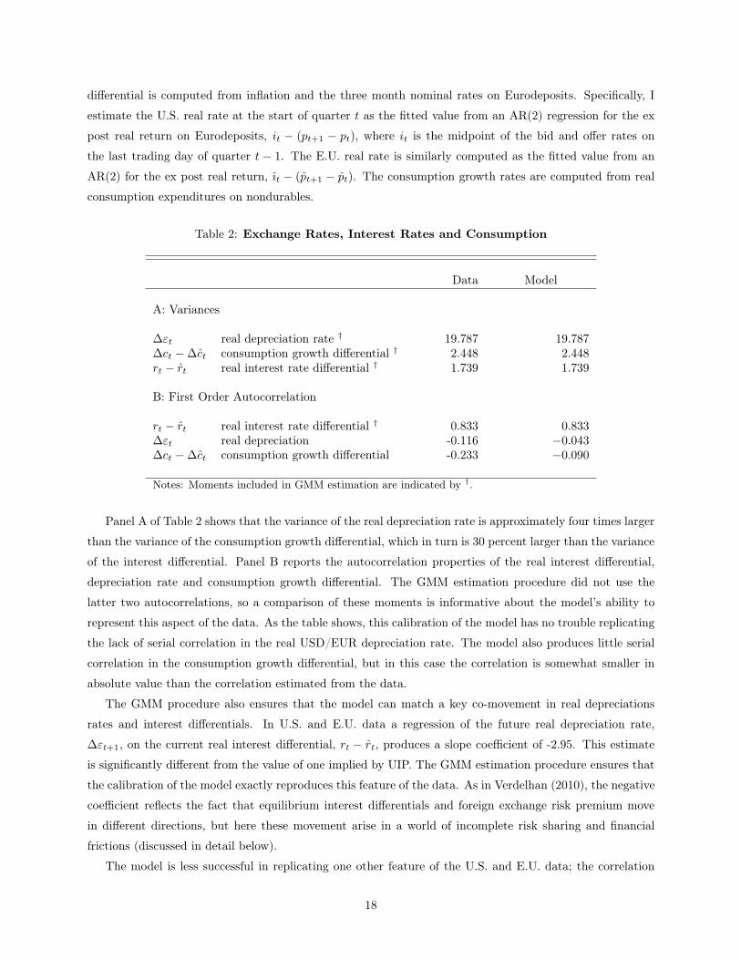
consumption expenditures on nondurables.

Table 2: Exchange Rates, Interest Rates and Consumption

Data Model

A: Variances

�"t

real depreciation rate † 19.787 19.787�c

t

��ct

consumption growth differential † 2.448 2.448rt

� rt

real interest rate differential † 1.739 1.739

B: First Order Autocorrelation

rt

� rt

real interest rate differential † 0.833 0.833�"

t

real depreciation -0.116 �0.043�c

t

��ct

consumption growth differential -0.233 �0.090

Notes: Moments included in GMM estimation are indicated by

†.

Panel A of Table 2 shows that the variance of the real depreciation rate is approximately four times larger

than the variance of the consumption growth differential, which in turn is 30 percent larger than the variance

of the interest differential. Panel B reports the autocorrelation properties of the real interest differential,

depreciation rate and consumption growth differential. The GMM estimation procedure did not use the

latter two autocorrelations, so a comparison of these moments is informative about the model’s ability to

represent this aspect of the data. As the table shows, this calibration of the model has no trouble replicating

the lack of serial correlation in the real USD/EUR depreciation rate. The model also produces little serial

correlation in the consumption growth differential, but in this case the correlation is somewhat smaller in

absolute value than the correlation estimated from the data.

The GMM procedure also ensures that the model can match a key co-movement in real depreciations

rates and interest differentials. In U.S. and E.U. data a regression of the future real depreciation rate,

�"t+1

, on the current real interest differential, rt

� rt

, produces a slope coefficient of -2.95. This estimate

is significantly different from the value of one implied by UIP. The GMM estimation procedure ensures that

the calibration of the model exactly reproduces this feature of the data. As in Verdelhan (2010), the negative

coefficient reflects the fact that equilibrium interest differentials and foreign exchange risk premium move

in different directions, but here these movement arise in a world of incomplete risk sharing and financial

frictions (discussed in detail below).

The model is less successful in replicating one other feature of the U.S. and E.U. data; the correlation

18

between the real depreciation rate, �"t

, and the consumption growth differential, �ct

� �ct

. The sample

correlation is -0.103, while in the model the unconditional correlation is -0.754. Producing a negative

correlation has long been a challenge for standard models using isoelastic time-separable utility with complete

markets (see, e.g., Backus and Smith, 1993), but here the combination of external habits and incomplete risk-

sharing produces too large a negative correlation. Unfortunately there does not appear to be an alternative

(reasonable) calibration of the model that produces a correlation between the real depreciation rate and

consumption growth differential closer to -0.1. while replicating the size of the UIP deviation and the

moments in Table 2.15

Habits

Habits are tightly linked to consumption in the calibrated equilibrium of the model. Recall that the level

of U.S. habit, Ht

, is related to the surplus ratio, St

, and aggregate consumption, Ct

, by the identity,

Ht

= (1�St

)Ct

. In equilibrium intertemporal smoothing by households ensures that aggregate consumption

responds immediately and one-for-one with shocks to the endowment trend. The log of equilibrium U.S.

consumption can therefore be represented as ct

= ct

+ccylt

, where ct

(=zt

) is the trend in consumption and

ccylt

is the remaining cyclical component driven by the temporary endowment shocks and the risk shocks.

Combing this decomposition with the definition of Ht

and using the fact that St

is stationary, we can

represent the dynamics of log U.S. habit by

ht

=

¯ht

+ hcyct

, where

¯ht

= ct

and hcyct

= ln(1� exp(st

)) + ccylt

.

Permanent shocks to consumption (i.e., shocks to ct

) are fully reflected in the level of habit via the trend

component ¯ht

. Other shocks affect the level of habit via the cyclical component hcyct

. In the C&C specifi-

cation, ccylt

= 0 and the log surplus ratio st

is driven by shocks to ct

. As I discuss below, in this model ccylt

varies in response to temporary endowment shocks and risk shocks because both shocks produce changes

in the terms of trade that affect households’ consumption decisions. As a result, even though risk shocks

directly affect the level of habit via their impact on the log surplus ratio, st

, they do not produce significant

variations in habit that are unrelated to consumption.

This feature can be seen from the time series representation of hcyct

. To derive the representation,

I first generate time series over 100,000 quarters for hcyct

and the innovations in cyclical consumption,

ccylt

� Et�1

ccylt

, from the model’s equilibrium. I then use these series to estimate the following ARMA15The problem of simultaneously replicating the size of UIP deviation, the volatility of real depreciation rates, and their

correlation with consumption growth differentials is long-standing in the literature. For example, Verdelhan (2010) replicatesthe anomaly but not the volatility of depreciation rates or their correlation with consumption. On the other hand, Colacitoand Croce (2011) have more success accounting for the volatility of depreciation rates and correlation with consumption, buttheir model cannot replicate the UIP deviation because it generates a constant market price of risk.

19

model:

hcyct

= 0.982hcyct�1

+ 1.061(ccylt

� Et�1

ccylt

)� 0.136(ccylt�1

� Et�2

ccylt�1

) + ✏t

, R2

= 0.954.

As the R2 statistic indicates, cyclical variation in habits are tightly tied to the history of consumption

innovations in the model’s equilibrium. Of course actual consumption innovations come from four different

shocks in the model which have different implications for the dynamics of habits and other variables. This

means that the estimated ARMA coefficients have no structural interpretation.16 They simply summarize

the fact that positive shocks to cyclical consumption are, on average, associated with higher levels of cyclical

habit that persist far into the future.

Returns on Foreign Assets and Liabilities

Table 3 compares the characteristics of U.S. foreign asset and liability returns with the foreign asset returns

generated by the model. The statistics on U.S. returns are based on the dataset from Evans (2012b)

that contains U.S. foreign asset and liability positions at market value and their associated returns at the

quarterly frequency. The data is constructed following procedures described in Gourinchas and Rey (2005)

that combine information on the market value for four categories of U.S. foreign asset and liabilities: Equity,

Foreign Direct Investment (FDI), Debt and Other; with information on the U.S. International Investment

Position reported by the Bureau of Economic Analysis.17 To facilitate comparisons with the model, the

table reports returns on two categories: “equity” that combines Equity and FDI, and “debt” that combines

Debt and Other. I also compute statistics for two sample periods: 1973:I-2007:IV and 1990:I-2007:IV. The

former period covers the entire post Bretton-Woods era prior to 2008 financial crisis, while the latter covers

the period after the adoption of the Euro used to compute the statistics in Table 2.

Columns (i) and (ii) of panels A and B report the sample means and standard deviations for log excess

returns on U.S. foreign assets, liabilities and their equity and debt components computed as rzj,t+1

� rt

,

where rzj,t+1

for z = {a, l} denotes the log real return on asset/liability j. Column (iii) reports Sharpe

ratios, computed as the sample average of gross excess returns, Rz

j,t+1

�Rt

, divided by their sample standard

deviation, while columns (iv) and (v) show the sample means and standard deviations of the portfolio shares,

↵zj,t

. Panel C reports analogous statistics computed from simulating the model over 100,000 quarters. Since

the model is symmetric, simulations of the U.S. foreign liability returns produce identical unconditional

moments.1816The estimated coefficients have extremely small standard errors, on the order of 0.003, so sampling error is not a concern

here. The estimates are also robust to adding further lags of hcylt and c

cylt � Et�1c

cylt .

17The Web Appendix provides details concerning the construction of the U.S. foreign asset and liability position data andthe associated returns.

18To be clear, the expected log excess return on the U.S. foreign asset portfolio is equal to the expected log excess return onthe U.S. foreign liability portfolio in the stochastic steady state of the model. So, long simulations produce average log excessreturns on foreign asset and liability portfolios that are identical (as are their sample variances). In contrast, my examinationof the external adjustment process below focuses on how endowment and risk shocks affect conditional expectations of futurelog returns, specifically conditional expectations concerning the differential between the log return on U.S. foreign assets andliabilities. Table 3 does not provide information on the dynamics of these conditional expectations in either the model or theU.S./E.U. data.

20

Table 3: Foreign Asset and Liability Returns

Mean Std. SharpeRatio

MeanShare

Std.Share Variance Contributions

Returns (i) (ii) (iii) (iv) (v) (vi) (vii) (viii)

A: 1973:I-2007:IV

All Assets 1.347 13.743 0.115 1.000 0.000 1.022 0.932 0.932Equity 1.960 26.927 0.108 0.483 0.105Debt -2.373 14.095 -0.149 0.517 0.105

All Liabilities 0.943 10.648 0.103 1.000 0.000 0.988 1.049 1.064Equity 1.805 27.806 0.103 0.361 0.073Debt -2.623 18.831 -0.113 0.639 0.073

B: 1990:I-2007:IV

All Assets 2.285 14.878 0.172 1.000 0.000 0.861 0.882 0.749Equity 3.187 25.566 0.158 0.568 0.061Debt -2.600 10.912 -0.221 0.432 0.061

All Liabilities 1.816 10.374 0.188 1.000 0.000 1.134 0.957 0.890Equity 3.261 24.046 0.168 0.418 0.052Debt -3.142 14.588 -0.194 0.582 0.052

C: Model

All Assets 3.471 19.764 0.176 1.000Equity 4.470 19.129 0.420 0.000Debt 0.000 17.127 0.580 0.000

Notes: The upper panels report statistics computed from U.S. data over the sample periods indicated. The lower panelreports statistics computed from the stochastic steady state of the model. Columns (i) and (ii) show the means andstandard deviations for log excess returns for all assets listed in the left hand column. All log returns are multiplied by400. Column (iii) reports the Sharpe ratios. Columns (iv) and (v) show the average and standard deviation of the shareof each asset and liability category in total assets and liabilities, respectively. Variance decompositions for the returns onU.S. foreign assets and liabilities are in the three right-hand columns. The variance contribution of returns using constantasset or liability shares, the average of asset and liability shares, and the constant average of asset and liability shares areshown in column (vi)- (viii), respectively.

.

An inspection of the table reveals that the sample statistics computed from the U.S. data are generally

comparable with those implied by the model. Log excess foreign asset returns in the model have a somewhat

higher mean and standard deviation than in the two data samples, but the Sharpe ratio implied by the

model closely matches the ratio computed in the second data sample. It is worth emphasizing that the

model’s equilibrium is calibrated to match the moments of exchange rates, interest rates and consumption

in Table 2 rather than the behavior of these returns, so some differences between the sample statistics in

Panels A and B and the model statistics are to be expected. Moreover, the U.S. data on returns comes from

21

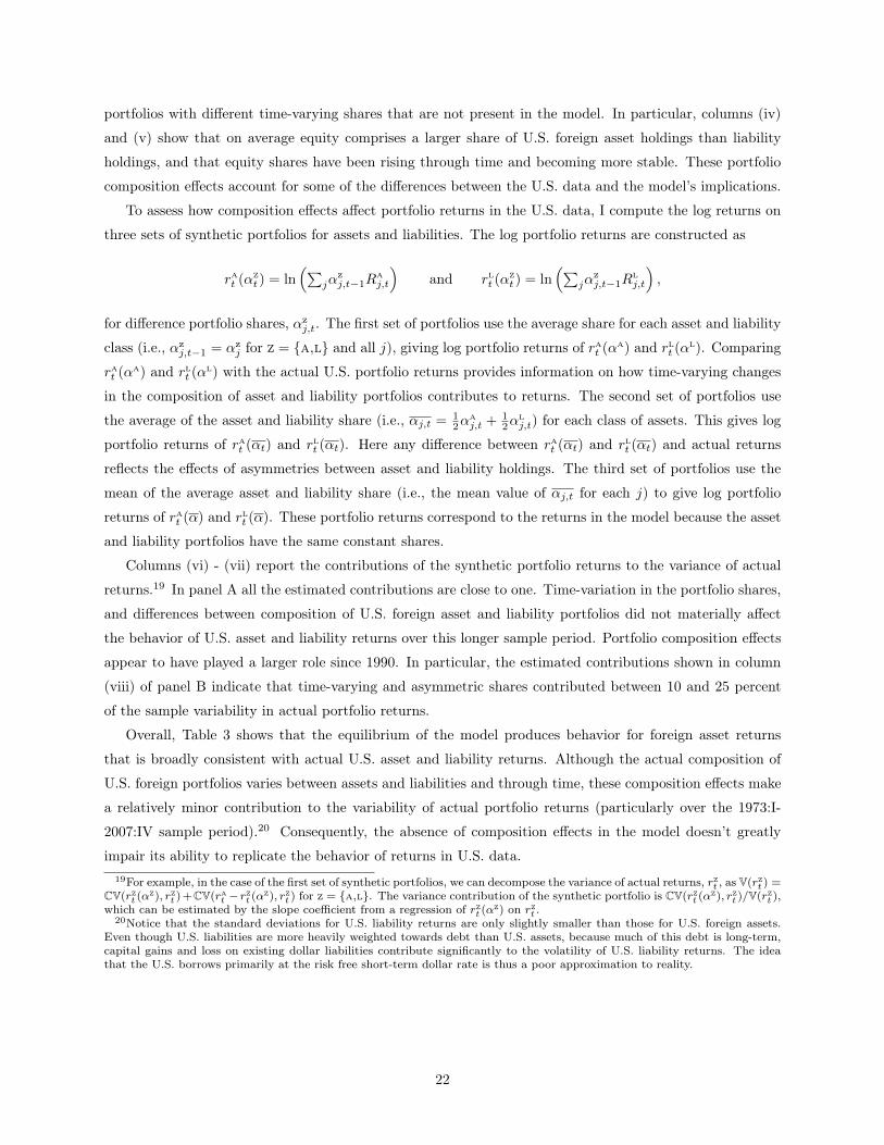
portfolios with different time-varying shares that are not present in the model. In particular, columns (iv)

and (v) show that on average equity comprises a larger share of U.S. foreign asset holdings than liability

holdings, and that equity shares have been rising through time and becoming more stable. These portfolio

composition effects account for some of the differences between the U.S. data and the model’s implications.

To assess how composition effects affect portfolio returns in the U.S. data, I compute the log returns on

three sets of synthetic portfolios for assets and liabilities. The log portfolio returns are constructed as

rat

(↵zt

) = ln

⇣

P

j

↵zj,t�1

Raj,t

⌘

and rlt

(↵zt

) = ln

⇣

P

j

↵zj,t�1

Rlj,t

⌘

,

for difference portfolio shares, ↵zj,t

. The first set of portfolios use the average share for each asset and liability

class (i.e., ↵zj,t�1

= ↵zj

for z = {a,l} and all j), giving log portfolio returns of rat

(↵a) and rl

t

(↵l). Comparing

rat

(↵a) and rl

t

(↵l) with the actual U.S. portfolio returns provides information on how time-varying changes

in the composition of asset and liability portfolios contributes to returns. The second set of portfolios use

the average of the asset and liability share (i.e., ↵j,t

=

1

2

↵aj,t

+

1

2

↵lj,t

) for each class of assets. This gives log

portfolio returns of rat

(↵t

) and rlt

(↵t

). Here any difference between rat

(↵t

) and rlt

(↵t

) and actual returns

reflects the effects of asymmetries between asset and liability holdings. The third set of portfolios use the

mean of the average asset and liability share (i.e., the mean value of ↵j,t

for each j) to give log portfolio

returns of rat

(↵) and rlt

(↵). These portfolio returns correspond to the returns in the model because the asset

and liability portfolios have the same constant shares.

Columns (vi) - (vii) report the contributions of the synthetic portfolio returns to the variance of actual

returns.19 In panel A all the estimated contributions are close to one. Time-variation in the portfolio shares,

and differences between composition of U.S. foreign asset and liability portfolios did not materially affect

the behavior of U.S. asset and liability returns over this longer sample period. Portfolio composition effects

appear to have played a larger role since 1990. In particular, the estimated contributions shown in column

(viii) of panel B indicate that time-varying and asymmetric shares contributed between 10 and 25 percent

of the sample variability in actual portfolio returns.

Overall, Table 3 shows that the equilibrium of the model produces behavior for foreign asset returns

that is broadly consistent with actual U.S. asset and liability returns. Although the actual composition of

U.S. foreign portfolios varies between assets and liabilities and through time, these composition effects make

a relatively minor contribution to the variability of actual portfolio returns (particularly over the 1973:I-

2007:IV sample period).20 Consequently, the absence of composition effects in the model doesn’t greatly

impair its ability to replicate the behavior of returns in U.S. data.19For example, in the case of the first set of synthetic portfolios, we can decompose the variance of actual returns, rzt , as V(rzt ) =

CV(rzt (↵z), r

zt )+CV(rat � r

zt (↵

z), r

zt ) for z = {a,l}. The variance contribution of the synthetic portfolio is CV(rzt (↵z

), r

zt )/V(rzt ),

which can be estimated by the slope coefficient from a regression of rzt (↵z) on r

zt .

20Notice that the standard deviations for U.S. liability returns are only slightly smaller than those for U.S. foreign assets.Even though U.S. liabilities are more heavily weighted towards debt than U.S. assets, because much of this debt is long-term,capital gains and loss on existing dollar liabilities contribute significantly to the volatility of U.S. liability returns. The ideathat the U.S. borrows primarily at the risk free short-term dollar rate is thus a poor approximation to reality.

22

Portfolios Shares

Table 4 reports the shares of domestic and foreign assets in households’ portfolios in the stochastic steady

state of the model. Column (i) reports the portfolio shares for the benchmark specification where } = 0.420,

the value calibrated from U.S. data. Column (ii) shows the steady state portfolio shares in an equilibrium

where } = 0.491. The shares of foreign equity and bonds in this equilibrium match the steady state shares in

an equilibrium where households freely choose the composition of their foreign asset portfolios (i.e., } = }⇤

as discussed in Section 2.1).21

Table 4: Steady State Portfolio Shares

Share Benchmark Optimal(} = 0.420) (} = 0.491)

(i) (ii)

Domestic Equity 0.937 0.926

Domestic Bonds -0.087 -0.076

Foreign Equity 0.063 0.074

Foreign Bonds 0.087 0.076

Notes: The table reports the shares of equity and bonds in household wealthin the stochastic steady state of the model under the benchmark calibration incolumn (i) and when } is chosen to maximize household utility in column (ii).

.

As Table 4 shows, the steady state of the model is characterized by a very high degree of equity home

bias. This feature of the model arises for two reasons. First, households receive all their income in the form

of dividends from domestic equity and their foreign asset holdings. As such, they are not concerned with

hedging non-tradable income risk. Following the logic in Baxter, Jermann, and King (1998), extending the

model to include non-tradable (wage) income in households’ budgets could lower the degree of equity home

bias. The second reason arises from the presence of the portfolio constraints. As I show below, holdings in

the foreign asset mutual fund provide domestic households with a poor hedged against risk shocks because

they suffer capital losses (via exchange rate appreciation) when marginal utility is unexpected high. In a

world without frictions (complete markets), households would hold equal long positions in domestic and

foreign equity to benefit from international diversification, and a short position in foreign bonds to hedge

against the adverse effects of domestic risk shocks. In the model, by contrast, the presence of the portfolio

constraint restricts households to either long or short positions in both foreign equity and bonds (as part

of their foreign fund holdings). As a consequence, the expected return on the foreign asset fund needs to

compensate for this lack of flexibility if households are to take large equilibrium positions. This level of21The portfolio shares in column (ii) are computed from the steady state in which the parameters in Panel B of Table 1 are

re-estimated by GMM to insure that the moments implied by the equilibrium also match the data as in Table 2.

23

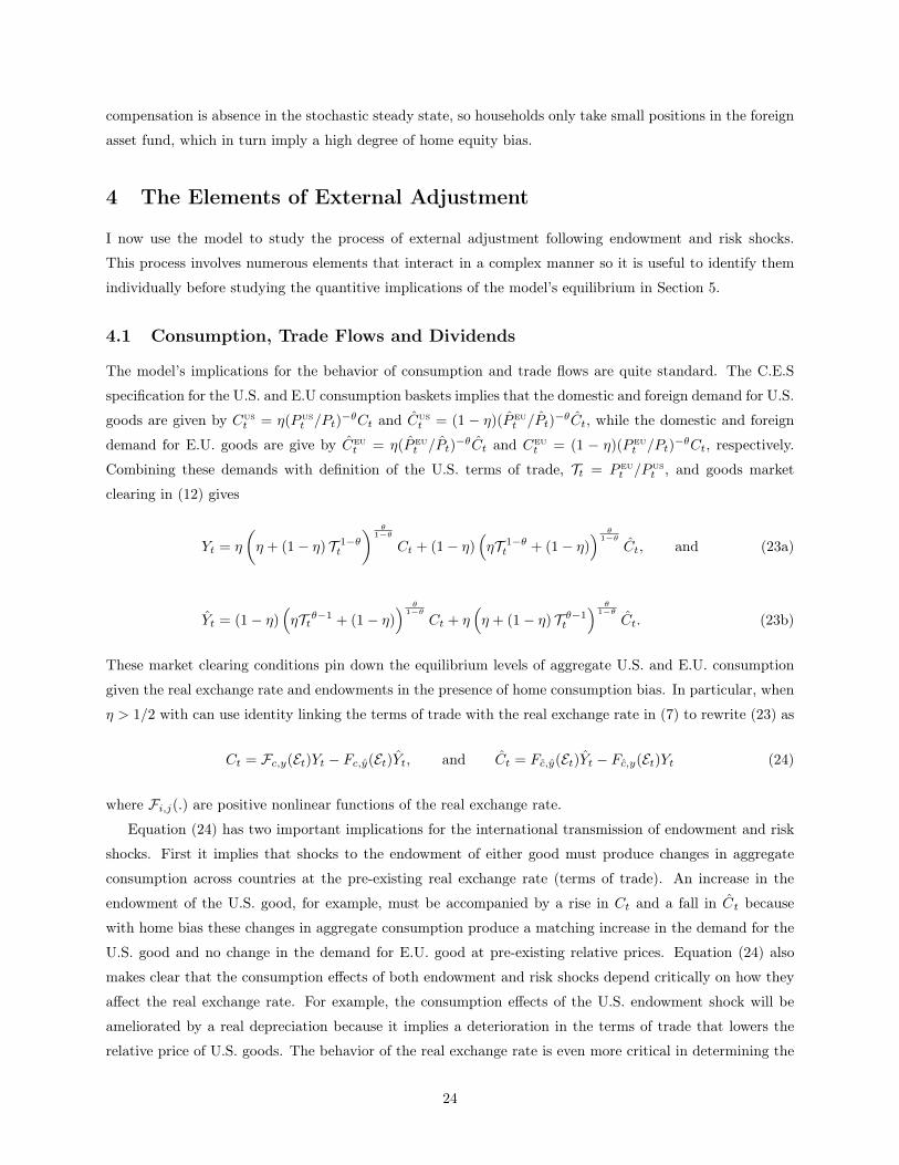
compensation is absence in the stochastic steady state, so households only take small positions in the foreign

asset fund, which in turn imply a high degree of home equity bias.

4 The Elements of External Adjustment

I now use the model to study the process of external adjustment following endowment and risk shocks.

This process involves numerous elements that interact in a complex manner so it is useful to identify them

individually before studying the quantitive implications of the model’s equilibrium in Section 5.

4.1 Consumption, Trade Flows and Dividends

The model’s implications for the behavior of consumption and trade flows are quite standard. The C.E.S

specification for the U.S. and E.U consumption baskets implies that the domestic and foreign demand for U.S.

goods are given by Cust

= ⌘(P ust

/Pt

)

�✓Ct

and ˆCust

= (1 � ⌘)( ˆP eut

/ ˆPt

)

�✓

ˆCt

, while the domestic and foreign

demand for E.U. goods are give by ˆCeut

= ⌘( ˆP eut

/ ˆPt

)

�✓

ˆCt

and Ceut

= (1 � ⌘)(P eut

/Pt

)

�✓Ct

, respectively.

Combining these demands with definition of the U.S. terms of trade, Tt

= P eut

/P ust

, and goods market

clearing in (12) gives

Yt

= ⌘

✓

⌘ + (1� ⌘) T 1�✓

t

◆

✓1�✓

Ct

+ (1� ⌘)⇣

⌘T 1�✓

t

+ (1� ⌘)⌘

✓1�✓

ˆCt

, and (23a)

ˆYt

= (1� ⌘)⇣

⌘Tt

✓�1

+ (1� ⌘)⌘

✓1�✓

Ct

+ ⌘⇣

⌘ + (1� ⌘) T ✓�1

t

⌘

✓1�✓

ˆCt

. (23b)

These market clearing conditions pin down the equilibrium levels of aggregate U.S. and E.U. consumption

given the real exchange rate and endowments in the presence of home consumption bias. In particular, when

⌘ > 1/2 with can use identity linking the terms of trade with the real exchange rate in (7) to rewrite (23) as

Ct

= Fc,y

(Et

)Yt

� Fc,y

(Et

)

ˆYt

, and ˆCt

= Fc,y

(Et

)

ˆYt

� Fc,y

(Et

)Yt

(24)

where Fi,j

(.) are positive nonlinear functions of the real exchange rate.

Equation (24) has two important implications for the international transmission of endowment and risk

shocks. First it implies that shocks to the endowment of either good must produce changes in aggregate

consumption across countries at the pre-existing real exchange rate (terms of trade). An increase in the

endowment of the U.S. good, for example, must be accompanied by a rise in Ct

and a fall in ˆCt

because

with home bias these changes in aggregate consumption produce a matching increase in the demand for the

U.S. good and no change in the demand for E.U. good at pre-existing relative prices. Equation (24) also

makes clear that the consumption effects of both endowment and risk shocks depend critically on how they

affect the real exchange rate. For example, the consumption effects of the U.S. endowment shock will be

ameliorated by a real depreciation because it implies a deterioration in the terms of trade that lowers the

relative price of U.S. goods. The behavior of the real exchange rate is even more critical in determining the

24

response of aggregate consumption to risk shocks. As (24) clearly shows, all the effects of risk shocks on

equilibrium consumption are transmitted via changes in the real exchange rate.

Aggregate consumption and the terms of trade govern international trade flows. By definition U.S.

exports and imports are determined by E.U. households’ demand for U.S. goods, and U.S. demand for E.U.

goods, respectively. So, when measured in terms of the U.S. consumption basket, U.S. exports and imports

are given by

Xt

= (1� ⌘)�

⌘Tt

1�✓

+ (1� ⌘)��1 E

t

ˆCt

and Mt

= (1� ⌘)�

⌘Tt

✓�1

+ (1� ⌘)��1

Ct

. (25)

In the stochastic steady state, Tt

= Et

= 1 and Ct

=

ˆCt

so these expressions simplify to Xt

= (1� ⌘) ˆCt

and

Mt

= (1� ⌘)Ct

and trade is balanced between the countries.

Recall that equities are claims to the endowments of U.S. and E.U. goods. In particular, one share of

U.S. equity entitles the holder to receive a dividend of Dt

= (P ust

/Pt

)Yt

, while one share of E.U. equity

receives a dividend of ˆDt

= (

ˆP eut

/ ˆPt

)

ˆYt

. Substituting for relative prices with the terms of trade produces

Dt

=

✓

⌘ + (1� ⌘) T 1�✓

t

◆

�11�✓

Yt

and ˆDt

=

⇣

⌘ + (1� ⌘) T ✓�1

t

⌘

�11�✓

ˆYt

. (26)

Clearly, endowment shocks have a direct impact on domestic dividends. They also have an indirect impact

via the terms of trade which also affects foreign dividends. In contrast, risk shocks only affect dividends via

the terms of trade. Dividends are also linked to domestic consumption and the trade balance. In particular,

equations (23) - (26) imply that

Dt

= Ct

+Xt

�Mt

, and ˆDt

=

ˆCt

+ (Mt

�Xt

)/Et

. (27)

Thus U.S. trade surpluses (Xt

> Mt

) push the dividends on U.S. equity above consumption and the dividends

on E.U. equity below consumption.

4.2 Asset Prices

Asset prices play three important roles in the external adjustment process. First, they determine household

wealth at pre-existing asset holdings. Shocks that produce unexpected changes in asset prices induce re-

valuations of household wealth that affect their consumption and saving decisions. Second, asset price

variations produce international capital flows as households re-balance their portfolio holdings of foreign

assets and liabilities. Changes in asset prices can also affect the risk premia and risk free rates by pushing

households towards their collateral constraints.

The prices of domestic equity are readily determined from the first-order conditions of households’ op-

timizing problems. Let Dt

/Qt

= 1/⇤eqt

denote the dividend-price ratio for U.S. equity. The first-order

condition governing optimal share of domestic equity in U.S. households’ portfolios implies that

⇤

eqt

= Et

Mt+1

(1 + ⇤

eqt+1

)

Dt+1

Dt

�

with Mt+1

= �

✓

Ct+1

Ct

◆��

✓

St+1

St

◆��

. (28)

25

Analogously, the first-order condition for E.U. households implies that

ˆ

⇤

eqt

= Et

"

cMt+1

(1 +

ˆ

⇤

eqt+1

)

ˆDt+1

ˆDt

#

with cMt+1

= �

ˆCt+1

ˆCt

!��

ˆSt+1

ˆSt

!��

, (29)

where ˆDt

/ ˆQt

= 1/ˆ⇤eqt

is the dividend-price ratio for E.U. equity. The prices of U.S. and E.U. equity,

measured in terms of domestic consumption, are therefore

Qt

= ⇤

eqt

Dt

and ˆQt

=

ˆ

⇤

eqt

ˆDt

. (30)

Endowment shocks and risk shocks affect equity prices in several different ways. First, risk shocks directly

affect the intertemporal marginal rates of substitution, Mt+1

and cMt+1

, that govern dividend-price ratios

via their impact on the surplus ratios, St

and ˆSt

. Intuitively, equity prices must change in response to

risk shocks to compensate for the uncertainty associated with future dividend flows. Risk shocks also affect

equity prices indirectly via their impact on the terms of trade, aggregate consumption and dividends in both

countries as discussed above. Similarly, endowment shocks to either good have a direct effect on equity prices

via dividends, and indirect effects via the terms of trade.

Shocks to the common trend in the endowments have a different effect on equity prices. They have a

one-to-one impact on the level of U.S. and E.U. consumption because households prefer smooth consumption

paths, so goods markets clear without any change in the terms of trade. This has two consequences. First,

current U.S. and E.U. dividends rise one-for-one with the endowment shock. Second, the shock has no effect

on dividend-price ratios because the conditional distributions of future consumption, dividend and surplus

growth remain unchanged. As a result, shocks to the common trend in the endowments have the same

proportional effect on U.S. and E.U. equity prices.

The real exchange rate also acts as an asset price in the model because it determines the domestic value of

the foreign asset mutual funds: i.e., FAt

= Et

(Beut

+

ˆQt

Aeut

) and dFAt

= (Qt

ˆAust

+

ˆBust

)/Et

. The equilibrium

real exchange rate is determined by the real interest differentials and the foreign exchange risk premium. Let

�t

= Et

"t+1

� "t

+ rt

� rt

define the foreign exchange risk premium (hereafter simply the “FX premium”).22

Rewriting this definition as a difference equation in "t

, solving forward, and applying the Law of Iterated

expectations produces

Et

= exp

�Et

1X

i=0

{rt+i

� rt+i

+ �t+i

}+ Et

"

!

, (31)

where " ⌘ lim

t!1 "t

. In the steady state of the model the real exchange rate equals unity so Et

" = 0.

Equilibrium variations in the real exchange rate must reflect changes in current and expected future real

interest differentials, rt+i

� rt+i

; and/or changes in current and expected future FX premia, �t+i

.

The equilibrium interest differential is determined by the first-order conditions governing the optimal22Some definitions of the risk premium also include one half the variance of the real depreciation rate to account for the fact

that we are dealing with log rather than gross returns. I use this simpler definition for clarity but fully account for the presenceof log returns when solving the model.

26

holdings of domestic bonds

1 = Et

[Mt+1

]Rt

+ Bt

and 1 = Et

h

cMt+1

i

ˆRt

+

ˆBt

, (32)

with Bt

= C�

t

S�

t

Lt

and ˆBt

=

ˆC�

t

ˆS�

t

ˆLt

, where Lt

and ˆLt

are the Lagrange multipliers on the collateral

constraints in (18c) and (20c), respectively. Like equity prices, endowment and risk shocks affect real

interest rates via their impact on the intertemporal marginal rates of substitution. They can also affect

interest rates via the collateral constraints. Shocks that change the value of foreign assets so that the

constraints bind produce positive values for Bt

and ˆBt

and push real rates down relative to Et

[Mt+1

] and

Et

[

cMt+1

]. Intuitively, households’ expected utility from additional borrowing exceeds the real interest rate

when the collateral constraint is binding. Notice, also, that portfolio constraints have no direct effect on real

interest rates. The conditions in (32) would still apply if households were able to freely choose their foreign

equity and debt holdings.

The equilibrium FX premium is similarly determined by combining the first-order conditions governing

households’ choice of domestic bonds and foreign asset holdings:

0 = Et

"

Mt+1

Et+1

ˆRt

Et

�Rt

!#

+ }Et

Mt+1

Et+1

Et

⇣

ˆReqt

� ˆRt

⌘

�

+ {Bt

, and (33a)

0 = Et

cMt+1

✓

Et

Rt

Et+1

� ˆRt

◆�

+ }Et

cMt+1

Et

Et+1

(Reqt

�Rt

)

�

+ { ˆBt

. (33b)

These equations identify how financial frictions play a role in the determination of the equilibrium FX

premium. The first term on the right-hand-side of each equation jointly determine the premium in an

equilibrium where households are free to choose their holdings of foreign bonds and equity directly, and

there are no collateral constraints. Financial frictions can push the FX premium away from this benchmark.

When collateral constraints are absent but households can only hold foreign assets indirectly via the foreign

asset fund, optimal portfolio choice requires that (33) holds with { = 0. In this case the equilibrium FX

premium will also depend on the riskiness of foreign equity returns, identified by the second terms on the

right-hand-side of (33). The size of these terms depends upon } and the degree of international risk sharing.

In an equilibrium where risk sharing is complete, the expectations terms equal zero, and the presence of the

portfolio constraint does not affect the equilibrium FX premium.23 When risk sharing is incomplete, the FX

premium must adjust so that households are compensated for the risk of holding foreign bonds and equities

so its size will depend on }. Things are more complex when both portfolio and collateral constraints are

present. First, the presence of collateral constraints impair international risk sharing, so the FX premium

adjusts to reflect the risk of holding foreign equity when } > 0. Second, the collateral constraints directly

affect the equilibrium expected excess return on the foreign asset fund via the last terms on the right-hand-23The first-order conditions governing the choice of domestic and bonds by U.S. and E.U. households imply that

Et [Mt+1(Reqt �Rt)] = 0 and Et[cMt+1( ˆR

eqt � ˆ

Rt)], respectively. Combining these expressions with the complete risk-sharingcondition, cMt+1 = (Et+1/Et)Mt+1, gives Et

hcMt+1

EtEt+1

(R

eqt �Rt)

i= 0 and Et

hMt+1

Et+1Et

⇣ˆ

R

eqt � ˆ

Rt

⌘i= 0, so the condi-

tions in (33) simplify back to the case without financial frictions.

27

side of (33). These terms are positive when the constraints bind. Ceteris paribus, this lowers the equilibrium

expected excess return on foreign assets and the FX premium. I examine the quantitative significance of

both financial frictions on the behavior of the equilibrium FX premium in Section 5.

4.3 Saving, Portfolio Holdings and Capital Flows

Households’ savings and portfolio decisions play a central role in the international transmission mechanism.

U.S. and E.U. households enter period t with real wealth Wt

and ˆWt

that comprises pre-existing holdings

of domestic equity, bond and foreign assets (chosen in period t � 1) valued at current asset prices, and the

period t dividend payments from their equity holdings.24 Households then choose how much of this wealth

to save, and how to allocate their savings across domestic bonds, equity and foreign assets. Together these

decisions determine households desired changes in asset holdings that drive international capital flows.

Endowment and risk shocks affect households’ consumption and savings decisions via the consumption-

saving ratios: Ct

/(Wt

� Ct

) = 1/⇤ct

and ˆCt

/( ˆWt

� ˆCt

) = 1/ˆ⇤ct

. Combining the households’ first-order

conditions with these definitions and the budget constraints in (18b) and (20b) produces

⇤

ct

= Et

Mt+1

(1 + ⇤

ct+1

)

Ct+1

Ct

�

and ˆ

⇤

ct

= Et

"

cMt+1

(1 +

ˆ

⇤

ct+1

)

ˆCt+1

ˆCt

#

. (34)

The level of saving and consumption in each country relative to beginning-of-period wealth are therefore

U.S.: Wt

� Ct

=

⇤

ct

1 + ⇤

ct

Wt

, Ct

=

1

1 + ⇤

ct

Wt

, and (35a)

U.S.: ˆWt

� ˆCt

=

ˆ

⇤

ct

1 +

ˆ

⇤

ct

ˆWt

, ˆCt

=

1

1 +

ˆ

⇤

ct

ˆWt

. (35b)

The equations display two noteworthy features: First, ceteris paribus, ⇤

ct

and ˆ

⇤

ct

rise when households

anticipate higher growth in their future consumption. As a result, household save a larger fraction of their

wealth, consistent with standard intertemporal consumption smoothing. Second, the Lagrange multipliers on

the collateral constraints are absent from (34). Financial frictions only affect households consumption/saving

decisions indirectly via their impact on the equilibrium intertemporal marginal rate of substitution and

prospective future consumption growth.

Savings decisions, portfolio choices and asset price variations all contribute to capital flows. Consider the

flows associated with foreign equity. By definition the value of E.U. equity and bonds in U.S. households’

portfolio are given by Et

ˆQt

Aeut

= }↵fat

(Wt

�Ct

) and Et

Beui,t

= (1� })FAt

, so the flows of equity and bonds

24The real value of dividend payments also depends upon the period t real exchange rate/terms of trade; see (26) above.

28

during period t are

Et

ˆQt

�Aeut

= ↵fat

}(Wt

� Ct

)� ↵fat�1

}(Wt�1

� Ct�1

)

Et

ˆQt

Et�1

ˆQt�1

= �↵fat

}(Wt

� Ct

) + }↵fat�1

"

�(Wt

� Ct

)�

Et

ˆQt

Et�1

ˆQt�1

� 1

!

(Wt�1

� Ct�1

)

#

, (36)

and

Et

�Beut

= ↵fat

(1� })(Wt

� Ct

)� ↵fat�1

(1� })(Wt�1

� Ct�1

)

Et

Et�1

= �↵fat

(1� })(Wt

� Ct

) + (1� })↵fat�1

�(Wt

� Ct

)�✓

Et

Et�1

� 1

◆

(Wt�1

� Ct�1

)

�

. (37)

The first term in the second line of each equation identifies the flow resulting from U.S. households’ desire to

alter the share of foreign assets in their savings. Variations in these flow components are perfectly correlated

across equity and bond flows because households cannot adjust the composition of their foreign asset holdings.

The second term in each equation identifies the effects of changing savings behavior via �(Wt

�Ct

) and the

effects of capital gains or losses on pre-existing positions. Notice that these portfolio rebalancing effects can

have differing affects on equity and bond flows. Real capital gains and losses on pre-existing equity positions

depend on the variations in foreign equity prices and the real exchange rate, while the gains and loses on

bonds depend only on changes in the real exchange rate.

Equations (36) and (37) identify U.S. gross capital outflows. By convention, negative outflows represent

the purchase of foreign assets by U.S. households which correspond to positive values for Et

ˆQt

�Aeut

and

Et

�Beut

. Purchases of U.S. equity and bonds by E.U. households, (Qt

/Et

)�

ˆAust

and (1/Et

)�

ˆBust

represent

positive U.S capital inflows, and are identified from E.U. households’ choice for ↵fat

, and savings, ˆWt

� ˆCt

in an analogous manner to (36) and (37).

5 Quantitative Analysis

I now use the model to study the external adjustment process following endowment and risk shocks. The

goal of this analysis is to quantify the roles played the trade and valuation channels in the model and to

compare them against their estimated contributions to external adjustment in the U.S.. To identify how

financial frictions affect the adjustment process, I compare the impulse responses to endowment and risk

shocks in the benchmark specification with the portfolio and collateral constraints against the responses in

an alternative specification where the portfolio constraint is the only financial friction.

5.1 Internal Adjustment

Figure 1 shows the impulse responses of consumption and the terms of trade following a positive shock to

the U.S. endowment process, and a negative shock to the U.S. log surplus ratio. These responses identify

the effect of a one standard deviation shock when the economy is initially in the stochastic steady state.

29

The solid plots show the responses of variables in the benchmark equilibrium where both financial friction

are present; responses from the equilibrium where portfolio constraints are the only friction are shown by

the dashed plots. Overall, the plots show that the presence of collateral constraints have little quantitative

impact on the reaction of consumption and the terms of trade to either endowment or risk shocks. In the

upper panel, the consumption and terms of trade responses are essentially identical. In the lower panel the

responses are smaller (in absolute value) when collateral constraints are present, but the differences are not

economically significant.

To develop the intuition behind the responses in Figure 1, it proves useful to consider how the financial

frictions affect the degree of international risk sharing. Recall from (24) that equilibrium consumption

depends on the endowments and the real exchange rate: Ct

= Fc,y

(Et

)Yt

�Fc,y

(Et

)

ˆYt

and ˆCt

= Fc,y

(Et

)

ˆYt

�Fc,y

(Et

)Yt

. In the absence of any financial frictions, households could trade the two equities and bonds to

completely share the idiosyncratic risks they face (i.e., markets would be dynamically complete) so the real

exchange rate would equalize marginal utilities internationally: Et

= (Ct

/ ˆCt

)

�

(St

/ ˆSt

)

� . This risk-sharing

condition and (24) pin down equilibrium aggregate consumption and the real exchange rate in terms of

the exogenous endowments and surplus ratios: i.e., Ccmt

= F(St

, ˆSt

, Yt

, ˆYt

), ˆCcmt

=

ˆF(St

, ˆSt

, Yt

, ˆYt

), and

Ecmt

= (F(St

, ˆSt

, Yt

, ˆYt

)/ ˆF(St

, ˆSt

, Yt

, ˆYt

))

�

(St

/ ˆSt

)

� .25

Now consider how the introduction of the portfolio restriction affects the equilibrium degree of interna-

tional risk sharing. If the processes for Ccmt

, ˆCcmt

and Ecmt

fail to satisfy the market clearing conditions and

the first-order conditions governing household decision-making with the portfolio constraints, their presence

must impair international risk sharing. Alternatively, if the conditions are satisfied, Ccmt

, ˆCcmt

and Ecmt

identify the consumption and real exchange rate processes in an equilibrium where the portfolio constraint is

present and risk sharing is complete. Assessing these alternatives is straightforward. Our examination of the

first-order conditions (32) and (33) in Section 4.2 showed that the presence of the portfolio constraints does

not affect real interest differentials and the FX premium if aggregate consumption in each country follow the

Ccmt

and ˆCcmt

processes. Consequently, the process for the real exchange rate implied by the present value

relation (31) matches Ecmt

, so the Ccmt

and ˆCcmt

processes satisfy the goods market clearing conditions in

(24). Thus, the Ccmt

, ˆCcmt

and Ecmt

processes satisfy the model’s equilibrium conditions when the portfolio

constraints are present, and allow for complete international risk sharing: i.e., Ecmt

= (Ccmt

/ ˆCcmt

)

�

(St

/ ˆSt

)

� .

In contrast, international risk sharing is incomplete in the equilibrium where both the portfolio and

collateral constraints are present (i.e. the benchmark specification). In this case the collateral constraints

affect the behavior of real interest rates and the foreign exchange risk premium even if consumption follow

the Ccmt

and ˆCcmt

processes, so the present value relation in (31) gives values for the real exchange rate

that differ from Ecmt

. Consequently, the Ccmt

, ˆCcmt

and Ecmt

process do not satisfy the model’s equilibrium

conditions when both financial frictions are present, so the actual equilibrium processes imply incomplete

risk sharing.

Understanding the economics behind the plots in Figure 1 is straightforward with this risk-sharing per-25More formally, from (24) aggregate consumption must satisfy Ct = Fc,y((Ct/ ˆ

Ct)�(St/ ˆSt)

�)Yt �Fc,y((Ct/ ˆ

Ct)�(St/ ˆSt)

�)

ˆ

Yt

and ˆ

Ct = Fc,y((Ct/ ˆ

Ct)�(St/ ˆSt)

�)

ˆ

Yt � Fc,y((Ct/ ˆ

Ct)�(St/ ˆSt)

�)Yt. Solving these equations gives C

cmt = F(St, ˆSt, Yt, ˆYt) and

ˆ

C

cmt =

ˆF(St, ˆSt, Yt, ˆYt).

30

Fig

ure

1:Im

puls

eR

espon

ses

ofC

onsu

mpti

onan

dth

eTer

ms

ofTra

de

Not

es:

The

uppe

ran

dlo

wro

ws

show

the

effec

tsof

apo

siti

vesh

ock

toth

eU

.S.e

ndow

men

tan

dne

gati

vesh

ock

toth

eU

.S.s

urpl

usra

tio,

resp

ecti

vely

.B

oth

shoc

ksar

eon

est

anda

rdde

viat

ion

inm

agni

tude

,and

thei

reff

ects

onth

een

dow

men

tan

dsu

rplu

sra

tio

are

show

nin

pane

lsA

and

C.S

olid

plot

sid

enti

fyth

ere

spon

ses

inth

ebe

nchm

ark

equi

libri

umw

ith

both

finan

cial

fric

tion

s,w

hile

dash

edpl

ots

iden

tify

the

equi

libri

umre

spon

sew

hen

port

folio

cons

trai

nts

are

the

only

fric

tion

.In

pane

lsB

and

Eth

epl

ots

wit

hbu

llets

iden

tify

the

path

sof

E.U

.con

sum

ptio

n,th

ose

wit

hout

iden

tify

U.S

.con

sum

ptio

n.T

heho

rizo

ntal

axis

mea

sure

sth

eti

me

elap

sed

sinc

eth

esh

ock

inye

ars.

31

spective. For example, a positive shock to the U.S. endowment (see Panel A) requires a deterioration in the

U.S. terms of trade (i.e., a rise in P eut

/P ust

, see Panel C) to maintain goods market clearing at pre-existing

consumption levels. This, in turn, implies a real depreciation of the dollar. So, from risk-sharing perspective,

there needs to be a rise in relative consumption, Ct

/ ˆCt

. Panel B of Figure 1 shows that this comes about

via a larger rise in U.S. consumption than the fall in E.U. consumption because home bias in consumption

(⌘ > 1/2) produces the higher demand for U.S. goods necessary to clear markets. Notice, also, that the

responses of consumption are essentially the same in both equilibria because the presence of the collateral

constraint does little to impair the ability of households to fully share risk following the endowment shock.

In principle endowment shocks produce capital gains and losses that drive households towards the collateral

constraints thereby pushing equilibrium real interest rates and the foreign exchange risk premium away from

adjustment paths that allow for complete risk sharing. In practice, these affects are very small when a typi-

cally sized endowment shock hits the economy in the steady state. Consequently, the equilibrium adjustment

paths for consumption, the real exchange rate and the terms of trade following such shocks are very similar

to paths in the equilibrium with just the portfolio constraint that permit complete risk sharing.

The presence of collateral constraints has a larger impact on the adjustments following risk shocks. The

lower panels of Figure 1 show the effects of positive U.S. risk shock that increases local curvature of U.S.

households’ utility by approximately 6.5 percent and temporarily lowers their surplus ratio (see Panel D).

From risk-sharing perspective, the risk shock must produce immediate appreciation in the real exchange rate

to equalize marginal utility across countries. This appreciation also induces an improvement in the U.S.

terms of trade in the presence of home bias (see Panel F), so there must be a rise in U.S. consumption and

fall in E.U. consumption to clear goods markets (see Panel E). In this case the presence of the collateral

constraints have a small effect on consumption and the terms of trade (real exchange rate) because they

dampen the response of the real interest differential and the FX premium (see below).

The left hand panels of Figure 2 show the responses of log dividends, dt

and ˆdt

; and equity prices, qt

and qt

; to the endowment and risk shocks. Panels A and B show that following the endowment shock there

is a rise in both U.S. and E.U. dividends, a large rise in U.S. equity prices and a small fall in E.U. equity

prices. Intuitively, the rise in U.S. dividends reflects the positive effect of the shock on U.S. output which is

partially offset by the deterioration in the U.S. terms of trade. In addition, the shock increases the expected

intertemporal marginal rate of substitution via its affects on U.S. consumption, producing a rise in the equity

price-to-dividend ratio ⇤

eqt

[see (28)], so U.S. equity prices rise more than dividends. The endowment shock

also affects E.U. dividends and equity prices via its affect on the terms of trade. In this case the deterioration

in the U.S. terms of trade raise E.U. dividends ( ˆDt

in line with Dt

) and lowers ˆ

⇤

eqt

via its impact on expected

future dividend and consumption growth. The net effect is a small fall in E.U. equity prices ˆQt

=

ˆ

⇤

eqt

ˆDt

(see Panel B).

Panels E and F show the effects of the risk shock. Here all the variations in dividends reflect the effect

of the improvement in the U.S. terms of trade that produce a temporary rise (fall) in the real value of U.S.

(E.U.) dividends. These valuation effects have very different impacts on equity prices. In the U.S., the

risk shock produces a large fall in ⇤

eqt

via expectations of lower intertemporal marginal rate of substitution

and dividend growth [see (28)] that overwhelm the effects of higher dividends, so U.S. equity prices fall. In

32

Fig

ure

2:Fin

anci

alM

arke

ts

Not

es:

The

uppe

ran

dlo

wer

row

ssh

owth

eeff

ects

ofth

epo

siti

vesh

ock

toth

eU

.S.

endo

wm

ent

and

nega

tive

shoc

kto

the

U.S

.su

rplu

sra

tio

depi

cted

inFig

ure

1.T

heve

rtic

alax

isin

each

plot

show

sth

ere

spon

sepe

ron

epe

rcen

tof

the

shoc

k.So

lidpl

ots

iden

tify

the

resp

onse

sin

the

benc

hmar

keq

uilib

rium

wit

hbo

thfin

anci

alfr

icti

ons,

whi

leda

shed

plot

sid

enti

fyth

eeq

uilib

rium

resp

onse

whe

npo

rtfo

lioco

nstr

aint

sar

eth

eon

lyfr

icti

on.

Inpa

nels

A-C

and

E-G

the

plot

sw

ith

bulle

tsid

enti

fyth

epa

ths

ofE

.U.va

riab

les,

thos

ew

itho

utid

enti

fyU

.S.

vari

able

s.T

heho

rizo

ntal

axis

mea

sure

sth

eti

me

elap

sed

sinc

eth

esh

ock

inye

ars.

33

contrast, the fall in E.U. dividends produces a small drop in equity prices because the combined effect of the

risk shock on expected E.U. consumption and dividend growth produces a small rise in ˆ

⇤

eqt

.

The right hand panels of Figure 2 show the responses of the log risk free rates, rt

and rt

, and the

FX premium, �t

. Panels C and D show that the endowment shock affects the risk free rates but not

the premium. Specifically, lower (higher) expected consumption growth following the shock (see Panel B

in Figure 1) produce a significant fall in the U.S. rate and small rise in the E.U. rate via intertemporal

smoothing. As in Figure 1, the responses in the benchmark equilibrium are very similar to those in the

equilibrium with only the portfolio constraint where risk sharing is complete. Panels G and H show how

real interest rates and the FX premium respond to the risk shock. Here, in contrast to Panels C and D,

the interest rate responses are far smaller than the premium response. Although the exact effects of the risk

shock on interest rates differ between the two equilibria, their (absolute) size amounts to a few basis points

whereas the FX premium rises by approximately 30 basis points. These differences imply quite different

adjustment mechanisms for real exchange rates. Recall from (31) that variations in the real exchange rate

must reflect changes in current and expected future real interest differentials and/or changes in the current

and expected FX premia. The responses shown here imply that risk shocks primarily affect the real exchange

rate via changes in the premia, while all the exchange-rate effects of endowment shocks are transmitted via

real interest differentials.

We can gain a better understanding of how different shocks affect interest rates and the FX premium

by considering the first-order conditions governing households’ portfolio choices. In the equilibrium without

collateral constraints, these conditions (approximately) imply that

rt

= � ln� + �Et

�ct+1

+ �Et

�st+1

� 1

2

�2Vt

(ct+1

+ st+1

), (38a)

rt

= � ln� + �Et

�ct+1

+ �Et

�st+1

� 1

2

�2Vt

(ct+1

+ st+1

), and (38b)

�t

=

1

2

�CVt

(ct+1

+ ct+1

, "t+1

) +

1

2

�CVt

(st+1

+ st+1

, "t+1

). (38c)

Following the U.S. endowment shock, households lower (raise) their expectations of future U.S. (E.U.) con-

sumption growth but not their forecasts for changes in the log surplus ratios or conditional second moments

involving consumption. Thus, the interest rates responses to the endowment shock in Panel B are entirely

produced by intertemporal smoothing via the second terms on the right-hand-side of (38a) and (38b), and

there is no change in the FX premium as shown by Panel D.

Risk shocks have more complex interest-rate effects. In particular, the U.S. risk shock raises both

�Et

�st+1

and �2Vt

(ct+1

+ st+1

) because U.S. households anticipate a future rise in the log surplus ra-

tio and greater volatility in marginal utility. These effects act on the equilibrium U.S. real interest rate in

opposite directions. The rise in �Et

�st+1

puts upward pressure on the real interest rate because households

want to borrow more, while in the increase in �2Vt

(ct+1

+ st+1

) induces greater precautionary saving. The

risk shock also lowers expectations of future U.S. consumption growth via its effects on the terms of trade.

These effects largely offset each other, so their combined impact on the U.S. real rate is very small (i.e., a

few basis points). Risk shocks also produce a small change in E.U. interest rates because the improvement in

the terms of trade induce a rise in �Et

�ct+1

. The small size of these interest-rate effects is not surprising. In

34

the C&C model the parameters of the habit process are chosen so that interest rates are constant. Here the

parameters are estimated so that the volatility of interest differentials match the data. This requires that

the intertemporal smoothing and precautionary savings effects of risk shocks on real interest rates largely

offset each other.

Risk shocks have significant effects of the FX premium because they change the hedging properties

of foreign asset portfolios. In particular, the U.S. risk shock produces a real appreciation of the dollar

that generates an unanticipated capital loss on the foreign asset holdings when U.S. marginal utility is

unexpectedly high. Thus, the expected equilibrium excess return on foreign assets must compensate U.S.

households for the poor hedge they provide against the adverse effects of future U.S. risk shocks. When the

U.S. risk shock hits, this compensation rises because the fall in st

makes marginal utility more sensitive to

future risk shocks [see (2)]. As a result, the expected excess return on U.S. foreign assets increases via a rise in

the FX risk premium.26 Equation (38c) identifies this hedging effect by an increase in CVt

(st+1

+ st+1

, "t+1

).

The right hand panels in Figure 2 show that the presence of collateral constraints only visibly affect the

interest-rate and FX risk premium responses to risk shocks. In particular, the fall in U.S. equity prices and

appreciation of the dollar reduces the collateral value of U.S. and E.U. households’ foreign asset holdings

which in turn lower interest rates by a few basis points. The fall in the collateral value of foreign asset

holdings also dampens the rise in the FX premium (again by a few basis points). Intuitively, equilibrium

expected excess returns need not rise as much to compensate for the deterioration in the hedging properties

of U.S. foreign assets when they also have collateral value.

One final aspect of Figure 2 deserves special comment. As I noted above, all the variations in the real

exchange rate induced by endowments shocks are produced by changes in current and expected future real

interest differentials because the shocks have no discernible effect on the FX premium (even when collateral

constraints are present). Consequently, the equilibrium dynamics of real depreciation rates and interest

differentials driven by endowment shocks are consistent with UIP: A regression of �"t+1

on rt

� rt

generated

by endowment shocks would produce a slope coefficient of one. In contrast, risk shocks produce variations

in the FX premium and interest differentials. Indeed, an inspection of Panels G and H reveals that rt

� rt

falls and �t

rises following the U.S. risk shock. More generally, risk shocks produce a negative correlation

between the real interest differential and the FX premium, and greater volatility in the FX premium than

the interest differential. These are the statistical properties necessary to produce a negative slope coefficient

from a regression of �"t+1

on rt

� rt

(see, e.g., Fama, 1984), so risk shocks must play an important role in the

GMM calibration of the model to replicate the coefficient of -2.95 estimated from U.S./E.U. data (together

with the other moments in Table 2).27

26Recall from Section 4.2 that the expected excess return on foreign assets equals the FX premium in the equilibrium withoutcollateral constraints.

27Although Figure 2 shows that endowment shocks produce no visible variations in the FX premia, this feature arisesendogenously in the model rather than directly from an specific assumption. In principle, endowment shocks could inducelarge enough changes in the value of foreign asset holdings to produce sizable variations in the FX premia in the benchmarkequilibrium with collateral constraints - via their effects on Bt and ˆBt in the first-order conditions (32) and (33). Calibrationsproducing such effects are implicitly considered by the GMM estimation procedure, but they are discarded in favor of thebenchmark calibration because it produces a match between the model moments and the data. In sum, the model allowsendowment shocks to produce variations in the FX premium, but it cannot do so without generating counterfactual behaviorfor exchange rates, consumption growth and interest rates.

35

5.2 External Adjustment

I now quantify the roles played the trade and valuation channels of external adjustment. First I derive a

simple approximation that links the U.S. foreign asset position to exports, imports and the returns on foreign

assets and liabilities. I then use this approximation to study how endowment and risk shocks affect the U.S.

net foreign asset position, and compare these implications of the model with estimates from U.S. data.

Net Foreign Assets, Trade and Returns

In the steady state of the model households hold long positions in domestic equity, and foreign assets, and

a short position in domestic bonds. Thus U.S. foreign assets comprise a portfolio of E.U. equity and bonds

with a real value of FAt

= Et

(Beut

+

ˆQt

Aeut

), while U.S. foreign liabilities comprise U.S. equity and bonds

held by E.U. households with a real value of FLt

=

ˆBust

+ Qt

ˆAust

(= Et

dFAt

). Combining these definitions

with the bond and equity market clearing conditions in (10) and (11); the aggregated budget constraint for

U.S. households in (8); and the equation for dividends in (27) gives

FAt

� FLt

= Xt

�Mt

�Rflt

FLt�1

+Rfat

FAt�1

, (39)

where Rflt

=

ˆRfat

(Et+1

/Et

) is the gross real return on U.S. foreign liabilities.

Equation (39) is the consolidated U.S. budget constraint that links changes in foreign assets and liabilities

to exports, imports and returns. These links place restrictions on the process of external adjustment. To

see how, let NFAt

= FAt

� FLt

and Rnfat

= (Rfat

FAt�1

� Rfat

FLt�1

)/NFAt�1

denote the value of and

return on the U.S. net foreign asset position. Using these definitions we can rewrite (39) as NFAt

=

Xt

�Mt

+Rnfat

NFAt�1

. Iterating this expression forward, and taking conditional expectations produces

NFAt

= �Et

" 1X

i=1

⇣

Q

i

j=1

Rnfat+j

⌘�1

(Xt+i

�Mt+i

)

#

+ lim

k!1Et

⇣

Q

k

j=1

Rnfat+j

⌘�1

NFAt+k

.

In the steady state of the model net foreign asset positions are zero, so the last terms on the right hand side

disappears leaving

NFAt

= �Et

" 1X

i=1

⇣

Q

i

j=1

Rnfat+j

⌘�1

(Xt+i

�Mt+i

)

#

. (40)

Thus, at any point in time, the value of the U.S. net foreign asset position must reflect households expectations

concerning the future path of net exports, Xt

�Mt

, and the returns on net foreign assets, Rnfat

.

Equation (40) identifies the international solvency constraint that must hold in any model where inter-

national Ponzi-schemes are ruled out. In a world where the only internationally traded asset is a single risk

free real bond with a constant return R, (39) simplifies to NFAt

= �Et

P1i=1

R�i

(Xt+i

�Mt+i

), so changes

in the net foreign asset position only reflect revisions in the expected future path of net exports. Under

these circumstances all external adjustments to shocks take place through the “trade channel”: that is via

changes in future net exports. Moreover, since the net foreign asset position simply reflects a country’s long

or short position in bonds, capital gains and losses on pre-existing net asset positions cannot play any role

36

in the adjustment process.

In this model equation (40) places a more complex set of restrictions on the adjustment process because

two bonds and two equities are traded internationally. As a consequence, shocks can induce revisions in

expected future returns on both foreign assets and liabilities, as well as net exports, and unexpected changes

in exchange rates and equity prices can produce capital gains or losses on pre-existing net foreign asset

positions. While (40) continues to hold in this more complex environment, examining how these factors

interact is considerably facilitated by considering an approximation.

To derive the approximation, I first rewrite (39) as

ln

✓

FAt

Rfat

FAt�1

�

1� Mt

Rfat

FAt�1

�◆

= ln

✓

FLt

Rflt

FLt�1

�

1� Xt

Rflt

FLt�1

�◆

+ ln

✓

Rflt

Rfat

FLt�1

FAt�1

◆

. (41)

In the stochastic steady state, exports and imports are constant shares of consumption, Xt

= (1� ⌘) ˆCt

and

Mt

= (1 � ⌘)Ct

; the returns on foreign assets and liabilities are equal and constant, Rfat

= Rflt

= Rft

; and

both foreign assets and liabilities are constant fractions of households savings, FAt�1

= ↵f(W

t�1

� Ct�1

)

and FLt�1

= ↵f(

ˆWt�1

� ˆCt�1

), where ↵f is the steady state value for the portfolio shares, ↵fat

and ↵fat

.

The steady state is also characterized by a constant common consumption growth rate g and savings-to-

consumption ratios, ⇤

ct

=

ˆ

⇤

ct

= ⇤

c. Under these circumstances, the terms in square brackets in (41) are

constants equal to = 1� (1�⌘) exp(g)

R

f↵

f⇤

c 2 (0, 1). Taking a first-order Taylor series approximation to the left-

and right-hand sides of (41) around the steady state, and simplifying the resulting expression produces

nfat

= �(1� )Et

nxt+1

� Et

(rfat+1

� rflt+i

) + Et

nfat+1

,

where nfat

= ln(FAt

/FLt

) and nxt

= ln(Xt

/Mt

) are the log ratios of foreign assets to liabilities and exports

to imports. Finally, I iterate forward and take conditional exceptions (noting that limk!1E

t

knfat+k

= 0)

to obtain

nfat

= nfatrt

+ nfavalt

where (42)

nfatrt

= �(1� )Et

1X

i=1

i�1nxt+i

and nfavalt

= �E1X

i=1

i�1

(rfat+i

� rflt+i

).

The approximation in (42) embodies the central features of the international solvency constraint in (40).

For example, (42) implies that a shock producing an upward revision in the expected future path for U.S. net

exports (i.e., a rise in Et

nxt+i

) must also produce either an fall in expected future returns on foreign assets

Et

rfat+i

, a rise in expected future liability returns Et

rflt+i

, and/or a fall in value of net foreign assets (i.e., a

fall in nfat

). In the special case were a single riskless bond is the only internationally traded asset, returns

on foreign assets and liabilities are equal so (42) simplifies to nfat

= nfatrt

= �(1 � )Et

P1i=1

i�1nxt+i

.

I refer to nfatrt

as the trade component of the net foreign asset ratio. The effects of revisions in expected

37

future returns are identified by the valuation component, nfavalt

.28

There are two main advantages to using (42) rather than (40) to study external adjustment. First, (42)

links trade flows and returns to the net foreign asset position via a linear present value relation rather than

through the complex nonlinear relation in (40). This facilitates the examination of how net foreign assets

behave in the model and in actual U.S. data. Second, expressions for the log returns on U.S. foreign assets

and liabilities are readily determined from the model’s equilibrium conditions. Variations in these returns

are empirically important, so it proves useful to examine their theoretical drivers in the model.

Drivers of the U.S. Net Foreign Asset Position

We can use the approximate solvency constraint in (42) and a VAR to study the U.S. external adjustment

process. The VAR is used to construct the forecasts for net exports, nxt

, and the return differentials,

rnfat

= rfat

� rflt

, that appear in the definitions of the trade and valuation components, nfatrt

and nfavalt

. I

then compare the actual movements in nfat

against these estimates of nfatrt

and nfavalt

derived from the

VAR.

I estimate the trade and valuation components with several VAR specifications. In the base specification

I estimate a VAR for three variables: the return differential, rnfat

; the growth differential between exports

and imports, �nxt

= �xt

��mt

; and the sum the log net asset position and exports, nxat

= nfat

+ nxt

. I

include the latter two variables because the U.S. time series for nxt

and nfat

are quiet persistent in the sample

period (1973:I to 2007:IV). The approximation in (42) implies that nxat

= �Et

P1i=1

i�1

(�nxt+i

+ rnfat+i

),

so shocks producing persistent variations in nxt

should have little impact on nxat

because they have small

effects on the near-term forecasts for �nxt

. In addition, I estimate VARs that include �xt

and �mt

instead

of �nxt

, as well as rfat

and rflt

instead of rnfat

. In all these specifications the returns on foreign assets and

liabilities are constructed from the actual U.S. portfolios with time-varying shares. To facilitate comparisons

between the U.S. data and the model, I also estimate VARs where the returns on assets and liabilities are

constructed from portfolios with constant shares equal to the sample average, rfat

(↵) and rflt

(↵) (as discussed

in Section 3.3).

Let Yt

=

˜AYt�1

+

˜Vt

represent the estimates of a VAR written in first-order form, where the vector Yt

appropriately stacks the current and lagged values of all the VAR’s variables, and ˜A is the companion matrix

of estimated VAR coefficients. I compute estimates of the trade and valuation components as

gnfatrt

= �ıtr ˜A(I � ˜A)

�1Yt

� nxt

and gnfavalt

= �ıval ˜A(I � ˜A)

�1Yt

,

where ıtr and ıval are vectors such the �nxt

= ıtrYt

and rnfat

= ıvalYt

.

By definition, nfat

=

gnfatrt

+

gnfavalt

+ ⇠t

, where ⇠t

is a composite error comprising the approximation

error in (42) and the estimation error associated with forecasting the future path for �nxt

and rnfat

from28Gourinchas and Rey (2007) derive a similar approximation to the dynamics in (39) around a deterministic trend path where

solvency is satisfied. Their approximation links the cyclical components of exports, imports and the foreign asset and liabilitypositions rather than the trade flows and positions themselves.

38

the VAR. We may therefore decompose the unconditional variance of the log net foreign asset ratio as

V(nfat

) = CV(gnfatrt

, nfat

) + CV(gnfavalt

, nfat

) + CV(⇠t

, nfat

),

where V(.) and CV(., .) denote the variance and covariance operators, respectively. The first term on the

right-hand-side identifies the variance contribution of the estimated trade component, the second identifies

the contribution of the valuation component. I estimate these contributions as the slope coefficient from the

OLS regression of the estimated component on nfat

:

gnfatrt

= �trnfat

+ ⇣trt

and gnfavalt

= �valnfat

+ ⇣valt

. (43)

By least squares, �tr= CV(gnfa

trt

, nfat

)/V(nfat

) and �val= CV(gnfa

valt

, nfat

)/V(nfat

) so the regression

coefficients provide estimates of the variance contributions. I also compute confidence bands for these

estimates using White (1980) heteroskedastic consistent standard errors.

Panel A of Table 5 reports estimates of nfat

variance decomposition for the U.S. between 1973:I and

2007:IV computed from different VAR specifications. In all cases I report results based on second-order

VARs, but I obtain similar results using first- and third-order ones as well. The left-hand column lists the

variables included in the VAR. The center columns report the estimates of �tr, �val and �tr+�val together

with their 95 percent confidence bands. The right-hand column of the table reports the value for used

to compute the nfat

components. The values for of 0.988 and 0.980 maximize �tr+ �val for the VAR

specifications in rows (1) and (2), respectively.

The results in Panel A show a consistent pattern in the estimated variance contributions of the trade and

valuation components across the different VAR specifications. In all cases the variations in the estimates of

the expected future return differentials contribute more to the sample variance of the log net foreign asset

ratio than the estimated revisions future trade flows.29 There are, however, some noteworthy differences

across the estimates based on different VAR specifications. Comparing rows (1) and (2) we see that the

variance contribution of the trade (valuation) component is larger (smaller) when based on separate VAR

forecasts for export and import growth and returns than when based on VAR forecast for net export growth

and return differentials. Although both VAR specifications generate estimates of the trade and valuation

components that account for almost all the sample variation in the nfat

(the estimates of �tr+ �val are

close to one), it is hard to precisely pin down how real-time forecasts of future trade flows and returns

differentials were changing over the sample period. The estimates in rows (3) and (4) provide information

on the importance of changes in the composition of U.S. asset and liabilities portfolios. Here I report results

derived from VARs that replace the returns on actual portfolios with the returns on asset and liability

portfolios where the share of equity are fixed at the sample average of 0.42. This restriction reduces the

estimated variance contributions of the valuation components. It also reduces the explanatory power of the

VAR for nfat

, as measured by the estimates of �tr+ �val, compared to their counterparts in rows (1) and

29Gourinchas and Rey (2007) estimate a smaller variance contribution (of approximately 30 percent) from the valuationcomponent in their decomposition of the cyclical component of nfat. If I replace nxat with a cyclical component estimatedwith the HP filter in my analysis, I also find a much small variance contribution from revisions in forecasts of future returndifferentials.

39

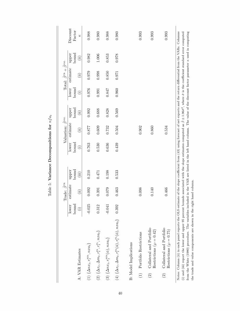
Tabl

e5:

Var

iance

Dec

ompos

itio

ns

fornfat

Trad

e:ˆ �tr

Val

uati

on:ˆ �va

lTo

tal:

ˆ �tr

+

ˆ �va

l

low

eres

tim

ate

uppe

rlo

wer

esti

mat

eup

per

low

eres

tim

ate

uppe

rD

isco

unt

boun

dbo

und

boun

dbo

und

boun

dbo

und

Fact

orA

:VA

RE

stim

ates

(i)

(ii)

(iii)

(i)

(ii)

(ii)

(i)

(ii)

(ii)

(1){�

nxt

,rnf

at

,nxat

}-0

.025

0.09

20.

210

0.76

30.

877

0.99

20.

976

0.97

90.

982

0.98

8

(2){�

xt

,�m

t

,rfat

,rflt

,nxat

}0.

312

0.39

10.

471

0.53

00.

609

0.68

80.

991

0.99

81.

006

0.98

0

(3){�

nxt

,rnf

at

(↵),n

xat

}-0

.041

0.07

90.

198

0.63

60.

732

0.82

80.

847

0.85

00.

853

0.98

8

(4){�

xt

,�m

t

,rfat

(↵),r

flt

(↵),n

xat

}0.

392

0.46

30.

533

0.43

90.

504

0.56

90.

960

0.97

10.

978

0.98

0

B:M

odel

Impl

icat

ions

(1)

Port

folio

Res

tric

tion

s0.

098

0.90

20.

993

(2)

Col

late

rala

ndPo

rtfo

lioR

estr

icti

ons

(}=

0.42)

0.14

00.

860

0.99

3

(2)

Col

late

rala

ndPo

rtfo

lioR

estr

icti

ons

(}=

0.75)

0.46

60.

534

0.99

3

Not

es:

Col

umn

(ii)

inea

chpa

nelr

epor

tsth

eO

LS

esti

mat

eof

the

slop

eco

effici

ent

from

(43)

usin

gfo

reca

stof

net

expo

rts

and

the

retu

rndi

ffere

ntia

lfro

mth

eVA

Rs.

Col

umns

(i)

and

(iii)

repo

rtth

elo

wer

and

uppe

r95

perc

ent

boun

dsas

soci

ated

wit

hth

esl

ope

esti

mat

esco

mpu

ted

asˆ

�±

1.96�

2,w

here

�is

the

coeffi

cien

tst

anda

rder

ror

com

pute

dfr

omth

eW

hite

(198

0)pr

oced

ure.

The

vari

able

sin

clud

edin

the

VA

Rar

elis

ted

inth

ele

ftha

ndco

lum

n.T

heva

lue

ofth

edi

scou

ntfa

ctor

para

met

er

used

inco

mpu

ting

the

trad

ean

dva

lue

com

pone

nts

are

show

nin

the

righ

tha

ndco

lum

n.

40

(2). This finding is consistent with the idea that real-time forecasts for future return differentials factor in

the effects of changing portfolio compositions.

Panel B of Table 5 reports values for �tr and �val implied by different equilibria of the model. These

values are computed from unconditional variances and covariances for nfat

, nfatrt

and nfavalt

using =

0.993, which is the value for implied by the model’s steady state. Rows (1) and (2) show that variations

in the valuation components account for high fractions of the variance in nfat

in the equilibrium with

the portfolio restriction (that permits complete risk sharing) and the equilibrium with both collateral and

portfolio constraints (that impair risk sharing). Indeed, the contribution of the valuation component in the

benchmark equilibrium in row (2) appears at the upper end of the range of estimates based on the U.S. data.

Of course these calculations are based on an equilibrium of a model that was calibrated to match the sample

moments of real exchange rates, interest rates and consumption growth differentials. It is not too surprising

that the values for �tr and �val implied by the external adjustment mechanism in the model do not exactly

match the estimates from U.S. data. Moreover, the values for �tr and �val implied by model appear to be

quite sensitive to the value for }, the share of equity in households’ foreign asset portfolios. For example,

row (3) shows that when } is set to 0.75, and all the other parameters are at their benchmark values, the

model’s equilibrium implies that �tr= 0.466 and �val

= 0.534.

Overall, the results in Table 5 show that variations in expected future return differentials between foreign

assets and liabilities made a major historic contribution to the variability of the U.S. net foreign asset ratio.

They also show that variations in expected future return differentials make a similarly important contribution

to the dynamics of the net foreign asset ratio in the model. As I noted in Section 2, this feature of the model

is new to the literature. To understand its theoretical foundation, I next consider how endowment and risk

shocks affect the value of net foreign assets via their impact on forecasts for future foreign asset returns and

trade flows.

Trade and Valuation Channels

Figure 3 shows the impulse responses of the log net export ratio, nxt

, the expected return differential on net

foreign assets, Et

rnfat+1

, the log net foreign asset ratio, nfat

, and its valuation component, nfavalt

. As above,

the solid plots show the responses of variables in the benchmark equilibrium where both financial friction are

present; responses from the equilibrium where portfolio constraints are the only friction are shown by the

dashed plots. Panels A-C plot the responses to the U.S. endowment shock. Recall that the shock produces

a rise in U.S. consumption and a deterioration in the U.S. term of trade. These effects produce a rise in U.S.

demand for E.U. goods and a fall in the E.U. demand for U.S. goods so nxt

initially falls before gradually

rising back to its steady state level as shown in Panel A. These plots also show that the adjustment path for

nxt

is not materially affected by the presence of the collateral constraints. Panel B plots the responses of

the expected return differential on U.S. foreign assets, Et

rnfat+1

= Et

(rfat+1

��"t+1

� rfat+1

). The endowment

shock has no effect on Et

rnfat+1

in the equilibrium without collateral constraints, but when they are present

there is a very small rise in Et

rnfat+1

(i.e., by a fraction of a basis point). Thus, most of the variation in the

value of U.S. net foreign asset position following an endowment shock occurs via the trade channel. This is

41

Fig

ure

3:Ext

ernal

Adju

stm

ent

Not

es:

The

uppe

ran

dlo

wer

row

ssh

owth

eeff

ects

ofth

epo

siti

vesh

ock

toth

eU

.S.

endo

wm

ent

and

nega

tive

shoc

kto

the

U.S

.su

rplu

sra

tio

depi

cted

inFig

ure

1.T

heve

rtic

alax

isin

each

plot

show

sth

ere

spon

sepe

ron

epe

rcen

tof

the

shoc

k.So

lidpl

ots

iden

tify

the

resp

onse

sin

the

benc

hmar

keq

uilib

rium

wit

hbo

thfin

anci

alfr

icti

ons,

whi

leda

shed

plot

sid

enti

fyth

eeq

uilib

rium

resp

onse

whe

npo

rtfo

lioco

nstr

aint

sar

eth

eon

lyfr

icti

on.

The

righ

tha

ndpa

nels

plot

the

resp

onse

sof

nfa

tw

itho

utci

rcle

s,an

dnfa

val

tw

ith

circ

les.

The

hori

zont

alax

ism

easu

res

the

tim

eel

apse

dsi

nce

the

shoc

kin

year

s.

42

illustrated by the responses for nfat

and nfavalt

plotted in Panel C.

These responses are consistent with the standard process of international adjustment that underlies the

intertemporal approach to the current account. In this case the transitory endowment shock produces capital

gains on U.S. households’ holdings of domestic equity and foreign assets that they use to raise consumption,

producing temporary current account deficits that are financed by higher dividends on their equity holdings.

As in a standard model, the adjustment of the net foreign asset position following the shock comes primarily

via the trade channel, but at the time the shock hits there are capital gains an losses on existing holdings.

Thus, unexpected valuation effects play a role in the external adjustment process following (temporary)

endowment shocks even though revisions in expect future trade flows account for most of the variations in

the net foreign asset position. The adjustment processes examined by Pavlova and Rigobon (2008), Tille

and van Wincoop (2010) and Devereux and Sutherland (2011) have these same features.

Panels D-F in Figure 3 show the external responses produced by the U.S. risk shock. Recall that this

shock induces a real appreciation of the dollar, a rise in U.S. consumption and a fall in E.U. consumption.

As a consequence there is a fall in the ratio of E.U. to U.S. consumption expenditure Et

ˆCt

/Ct

, and a rise in

the share of spending on U.S. goods in each country’s consumption basket. These factors affect net exports

in opposite directions, but in both equilibria the latter factor dominates producing the rise in nxt

shown in

Panel D. Notice that this trade response is smaller (in absolute value) than the response to the endowment

shock. In contrast, the risk shock has a much larger effect on the expected return differential, Et

rnfat+1

. As

Panel E shows, the presence of collateral constraints dampens the rise in Et

rnfat+1

by approximately 50 percent,

but it is still 25 times larger than the rise produced by the endowment shock. The response of the U.S. net

foreign asset ratio are shown in Panel F. Here we see the valuation component, nfavalt

, accounts for the

lion’s share of the nfat

responses in both equilibria. Since nfavalt

equals the presence value of expected

future return differentials, the Et

rnfat+1

responses in Panel E translate into sizable nfavalt

variations. In fact

the initial effect of the risk shock on nfat

in the benchmark equilibrium is roughly twice the (absolute) size

of the effect produced by the endowment shock.

The plots in Figure 3 reconcile the results in Table 5 and the analysis of the adjustment process following

endowment and risk shocks. Specifically, the small value for �tr and large value �val implied by the model’s

equilibrium arise because: (i) risk shocks affect the net foreign asset ratio primarily through the valuation

channel (i.e., via changes in Et

rnfat+1

that drive variations in nfavalt

), and (ii) they are the dominant source

of cyclical dynamics in the model. In contrast, (temporary) endowments shocks induce adjustment via the

trade channel and through unexpected valuation effects, so they cannot account for the estimates of �tr and

�val from U.S. data reported in Panel A of Table 5 unless they are unimportant drivers of cyclical U.S./E.U.

dynamics; which is, of course, consistent with the GMM estimates of the model.

To understand why the valuation channel is so important in the external adjustment process following

risk shocks, it proves useful to consider the links between the FX and equity risk premia and the expected

returns on the foreign asset mutual funds. Following Campbell and Viceira (2002), these returns can be

43

approximated by

rfat+1

= rt

+�"t+1

+

1

2

}(1� })Vt

�

reqt+1

�

+ }(reqt+1

� rt

) and

rfat+1

= rt

��"t+1

+

1

2

}(1� })Vt

�

reqt+1

�

+ }(reqt+1

� rt

).

Subtracting the log of the domestic real interest rate from each equation, and combining the results with

the definition of the FX premium, �t

, produces

Et

rfat+1

� rt

= �t

+ } brpeqt

� 1

2

}2Vt

�

reqt+1

�

and (44a)

Et

rfat+1

� rt

= ��t

+ }rpeqt

� 1

2

}2Vt

�

reqt+1

�

, (44b)

where rpeqt

= Et

reqt+1

� rt

+

1

2

Vt

(reqt+1

) and brpeqt

= Et

reqt+1

� rt

+

1

2

Vt

(reqt+1

) are the U.S. and E.U. equity

premia.30 In equilibrium these premia are determined by the first-order conditions governing households’

domestic equity and bond holdings [see (28), (29) and (32)], and are well-approximated by

rpeqt

=�CVt

(reqt+1

, ct+1

+ st+1

)� ln(1� Bt

), and (45a)

brpeqt

=�CVt

(reqt+1

, ct+1

+ st+1

)� ln(1� bBt

). (45b)

Finally, combining (44) with the definition of the return differential, rnfat+1

= rfat+1

��"t+1

� rfat+1

, gives

Et

rnfat+1

= �t

+ }⇥

brpeqt

� rpeqt

⇤

+

1

2

}2

⇥

Vt

�

reqt+1

�

� Vt

�

reqt+1

�⇤

. (46)

These equations provide the key to understanding why the valuation channel plays such different roles

following endowment and risk shocks. Consider first the effects of the endowment shock. Recall from Figure

2 that the shock has no effect on the FX premia in either equilibrium so the valuation channel will only

be operable if the shock changes Et

rnfat+1

via the equity risk premia, rpeqt

and brpeqt

, or the variance terms in

(46). Equation (45) shows that the equilibrium equity risk premia compensate for the hedging properties of

equities identified by the covariance terms, and the effects of the collateral constraints via Bt

and bBt

. When

the constraints are absent, the endowment shock has no affect on the conditional second moments so there is

no change in the equity premia in (45), or the variance terms in (46). As a result there is no revision in the

expected return differentials (i.e., Et

rnfat+i

for i > 0), so the valuation channel remains inoperable. When the

collateral constraints are present, the capital loss suffered by E.U. households on their foreign asset holdings

drives down rt

thereby raising the E.U. equity premium via the last term on the right-hand-side of (45b).

This produces a rise in Et

rfat+1

� rt

[see (44a)] which is reflected in Et

rnfat+1

, but the effect is extremely small,

30As is standard, I include the Jensen inequality terms, 12Vt(r

eqt+1) and 1

2Vt(reqt+1), to account for the fact that we are working

with log returns.

44

as was seen in Panel B of Figure 3. Consequently, the valuation channel plays almost no role in the external

adjustment process following (temporary) endowment shocks even when collateral constraints are present.

In contrast, the valuation channel plays an important role in the adjustment process following risk shocks

for three reasons: First, as discussed above, risk shocks have sizable affects on the FX premium because they

change the hedging properties of foreign bonds. Recall from Figure 2 that the U.S. risk shock had a larger

effect on �t

than on the real interest differential in both equilibria. These effects are directly reflected in

Et

rnfat+1

via the first term on the right-hand-side of (46). Second, risk shocks change the hedging properties

of equities. Recall that the U.S. risk shock produced an unanticipated fall in U.S. equity prices when U.S.

marginal utility was unexpectedly high, so the increased likelihood of further risk shocks must produce a rise

in the U.S. equity premium to compensate. This hedging effect is identified by an increase in the covariance

term on the right-hand side of (45a). U.S. risk shocks have minimal effects on E.U. equity prices and marginal

utility, so hedging properties of E.U. equity remain almost unchanged. In the equilibrium without collateral

constraints, the rise in rpeqt

dampens the effects of the higher FX premium on the expected return differential

so the rise in Et

rnfat+1

(see Panel C of Figure 3) is smaller than the rise in �t

(see Panel H of Figure 2). In

the equilibrium with collateral constraints, the dampened effects of the equity premia on Et

rnfat+1

are larger.

In this case, the capital losses U.S. households suffer on their foreign asset position drive the U.S. equity

premium even higher so that the effect of the risk shock on the expected return differential is reduced by

approximately 50 percent (see Panel E of Figure 3).

5.3 Asset Holdings and Capital Flows

I now turn to the remaining aspect of the external adjustment process, the behavior of capital flows. Panel

A in Table 6 reports the unconditional standard deviations from simulations of the benchmark equilibrium

with both portfolio and collateral constraints and from the equilibrium with just the portfolio constraints

for U.S. log savings, wt

� ct

; the log value of U.S. foreign assets, fat

; the U.S. portfolio shares for domestic

equity and foreign assets, ↵eqt

and ↵fat

; and the U.S. capital outflows for bonds and equity, Et

�Beut

and

Et

ˆQt

�Aeut

. These statistics show that the presence of collateral constraints has little impact on the volatility

of savings. This is consistent with the similarity of the impulse responses for consumption, dividends and

trade flows across in the different equilibria depicted in Figures 1-3. Households find it optimal in the

presence of collateral constraints to approximate the real consumption and savings decisions they would

make under complete markets. The constraints play a larger role on households’ financial decisions. As

the ratios in column (iv) show, the volatility of the U.S. foreign asset position is approximately 20 percent

higher when both constraints are present. By definition fat

= ln↵fat

+wt

� ct

, so the higher volatility in fat

induced by the financial frictions reflects more variability in households’ choice for ↵fat

. In fact the standard

deviations of both the foreign asset and domestic equity portfolio shares are approximately 15 percent higher

in the benchmark equilibrium. The presence of collateral constraints also raises the standard deviations of

U.S. capital outflows by approximately 10 percent. Bond flows are more volatile than equity flows in both

equilibria because the share of E.U. equities in U.S. foreign assets is fixed at } = 0.42. The volatility of

equity outflows is higher than bond outflows in equilibria with } > 0.5.

45

Table 6: Capital Flows

Variables Equilibria Ratio

Portfolio andCollateral Constraints Portfolio Constraints

(i) (ii) (iii) (iv)

A: Standard Deviations

wt

� ct

0.302 0.297 1.016

fat

0.782 0.654 1.195

↵eqt

0.089 0.077 1.155

↵fat

0.212 0.183 1.158

Et

�Beut

0.167 0.152 1.098

Et

ˆQt

�Aeut

0.120 0.109 1.101

B: Return Chasing Contributions

Bond Flows: Et

�Beut

0.717 0.714

Equity Flows: Et

ˆQt

�Aeut

1.381 1.381

Notes: Panel A reports the unconditional standard deviation from simulations of the benchmarkequilibrium with portfolio and collateral constraints in column (ii) and the equilibrium with justportfolio constraints in column (iii) for the variables listed in column (i). Column (iv) reports theratio of the statistics in columns (ii) to (iii). Panel B reports the variance contribution of the returnchasing components in U.S. foreign bond flows and equity flows in the benchmark and completemarkets equilibria. All statistics are computed from simulations spanning 100,000 quarters.

The statistics in Panel B identify the contribution of U.S. households’ portfolio reallocation decisions to

U.S. capital outflows. Recall from equations (36) and (37) that a portion of the equity and bond outflow,

Et

ˆQt

�Aeut

and Et

�Beut

, can be attributed to the change in the portfolio share ↵fat

: i.e., �↵fat

}(Wt

� Ct

)

and �↵fat

(1 � })(Wt

� Ct

). Panel B reports the variance contributions of these so-called “return chasing

contributions” to the bond and equity outflows. Even though these components are perfectly correlated

across the flows, their variance contributions are quite different because the effects of capital gains and losses

on pre-existing foreign bond and equity positions differs. Notice, also, that the variance decompositions are

almost identical across the two equilibria. The presence of collateral constraints raise the volatility of capital

outflows but has little affect on the role played by portfolio reallocations.31

31These variance decomposition results are similar to the findings reported elsewhere in the literature. For example, Tilleand van Wincoop (2010) find that changes in portfolio shares are an important driver of flows following endowment shocksin a model where only equity is traded internationally. Similarly, Evans and Hnatkovska (2013) show that the return chasingcomponent contributes most to the variance of bond and equity flows driven by productively shocks in a model with incomplete

46

We can study the role of capital flows in the external adjustment process in greater detail with the aid

of Figure 4. Here I plot the impulse responses of U.S. and E.U. bond and equity holdings following the

endowment and risk shocks. Each panel shows the percent deviation from the steady state holdings. For

example, Panel A plots the deviations in U.S. holdings of U.S. bonds, 100 ⇥ (Bust

� ¯Bust

)/ ¯Bust

, and the

deviations in E.U. holdings of E.U. bonds, 100⇥ (

ˆBeut

� ¯

ˆBeut

)/¯

ˆBeut

, where bars indicate steady state values.

As above, the upper and lower panels show the responses following the endowment and risk shocks. The

solid lines indicate the responses in the benchmark equilibrium with portfolio and collateral constraints and

the dashed lines show the responses in the equilibrium with only the portfolio constraints.

Two features of the plots in Figure 4 immediately stand out: First, the changes in bond and equity

positions following endowment shocks are extremely small and are far smaller than the changes induced by

the risk shocks. Since Et

ˆQt

�Aeut

, Et

�Beut

, (Qt

/Et

)�

ˆAust

and (1/Et

)�

ˆBust

represent U.S. capital outflows and

inflows for equities and bonds, the capital flows produced by endowment shocks must be very small. Indeed,

it turns out that endowment shocks account for less than one percent of the variance in bond and equity flows

produced by simulations of both equilibria. Thus, capital flows appear to play an insignificant role in the

adjustment process following endowment shocks. Intuitively, endowment shocks are typically too small to

affect equilibrium risk premia so households keep their portfolio shares constant.32 As a consequence, when

the shock hits U.S. households issue more domestic bonds to balance the capital gains on their pre-existing

domestic equity and foreign asset positions. The corresponding change in the U.S. and E.U. bond positions

are shown in panels A and B of Figure 4. This small bond flow is sufficient to finance the initial U.S. current

account deficit that follows the endowment shock. It is then reversed as U.S. households buy back the their

bonds with the proceeds of higher domestic dividends.

The second striking feature in Figure 4 appears in the lower panels. Here we see that the initial changes in

the foreign bond and equity positions produced by risk shocks are economically large, and are approximately

twice the size when collateral constraints are present. These position changes are an important driver of

bond and equity capital flows. In particular, the plots in panels F and H show that risk shocks induce sharp

initial falls in foreign bond and equity positions of both U.S. and E.U. households. They therefore represent

large positive bond and equity foreign capital outflows across the world economy.

To understand the source of these capital flows, recall that the U.S. risk shock produces a real appreciation

of the dollar and a fall in the domestic value of E.U. equity. Thus, E.U. equity holdings contribute more to

the capital loss U.S. households sustain on their foreign asset portfolio than do E.U. bonds. If households

were free to choose the composition of their foreign asset portfolio, the risk shock would produce a larger risk

premium on foreign equity than bonds to compensate U.S. households for their inferior hedging properties in

the face of future risk shocks. However, since the composition of the portfolio is fixed, the risk shock raises

the equilibrium expected excess return on the foreign assets instead; i.e., Et

rfat+1

� rt

[see (44a)], but not

enough to fully compensate U.S. households for the higher risk associated with holding E.U. equity, so they

markets.32Of course it is possible that an endowment shock hits when households are already close to their collateral constraints so

that the equilibrium risk premia and portfolio shares change. Under these circumstances, the shock would produce a morecomplex pattern of capital flows, but the simulations indicate that such patterns are very rare.

47

Fig

ure

4:Fo

reig

nA

sset

Hol

din

gsan

dC

apit

alFlo

ws

Not

es:

The

uppe

ran

dlo

wer

row

ssh

owth

eeff

ects

ofth

epo

siti

vesh

ock

toth

eU

.S.e

ndow

men

tan

dne

gati

vesh

ock

toth

eU

.S.s

urpl

usra

tio

depi

cted

inFig

ure

1.T

heve

rtic

alax

isin

each

plot

show

sth

ede

viat

ion

inpe

rcen

tfr

omth

est

eady

stat

eas

set

hold

ings

.So

lidpl

ots

iden

tify

the

resp

onse

sin

the

benc

hmar

keq

uilib

rium

wit

hbo

thfin

anci

alfr

icti

ons,

whi

leda

shed

plot

sid

enti

fyth

eeq

uilib

rium

resp

onse

whe

npo

rtfo

lioco

nstr

aint

sar

eth

eon

lyfr

icti

on.

Plo

tspl

ots

wit

hbu

llets

iden

tify

the

path

sof

E.U

.var

iabl

es,t

hose

wit

hout

iden

tify

U.S

.var

iabl

es.T

heho

rizo

ntal

axis

mea

sure

sth

eti

me

elap

sed

sinc

eth

esh

ock

inye

ars.

48

reduce their exposure to foreign assets by lowering ↵fat

.33 When coupled with the fall in U.S. saving, this

portfolio reallocation produces an 8 percent fall in U.S. holdings of foreign bonds and equity, as shown by the

dashed black plots in panels F and H of Figure 4. Similarly, the rise in Et

rfat+1

� rt

under-compensated E.U.

households for the higher risk of future capital losses on U.S. equity, so they reduce their exposed to foreign

assets by lowering ↵fat

. Although E.U. households savings remain relatively stable (because the capital loss

on U.S. equity is offset by the exchange rate), the fall in ↵fat

and appreciation of the dollar produce a fall in

E.U. holdings of U.S. bonds of approximately 12 percent (see Panel F).

Collateral constraints amplify the effects of the risk shocks on capital flows. The U.S. risk shock produces

capital losses on pre-existing U.S. equity and foreign asset positions as well as a desired portfolio reallocation

that lowers ↵fat

. Together, these effects lower the value of foreign asset holdings that can be used as collateral

when issuing U.S. bonds. In response, U.S. households sell a larger fraction of their foreign asset portfolio

in order to buy back more outstanding U.S. bonds. These actions produce the larger U.S. capital outflows

depicted in panels F and H of Figure 4. The reallocation of E.U. portfolios has a similar collateral effect on

E.U. outflows. In this case the fall in ↵fat

reduces the value of foreign assets available for E.U. households

to use when issuing E.U. bonds. And, as a result, E.U. households sell foreign assets to buy back previously

issued domestic bonds. As Figure 4 shows, the size of the E.U. bond and equity outflows produced by these

transactions are very similar to their U.S. counterparts.

Table 7: U.S. Asset and Liability Position Changes

Equity Assets Debt Assets EquityLiabilities

Debt Liabilities

Equity Assets - 0.682 0.903 0.440Debt Assets 0.399 - 0.611 0.847

Equity Liabilities 0.877 0.298 - 0.383Debt Liabilities -0.015 0.617 -0.062 -

Notes: The table reports correlations between changes in U.S. foreign asset and liability positions at theannual frequency above and quarterly frequency below the leading diagonal. All positions are valued atmarket prices converted to constant dollars. Correlations are computed from the 1973:I-2007:IV sampleperiod.

Finally, it is instructive to compare the dynamics of foreign asset and liability holdings in the model

with actual changes in U.S. foreign asset and liability positions. Table 7 reports the correlations between

quarterly and annual changes in gross U.S. asset and liability positions in equity and debt in the post Bretton-

Woods era. Here we see that annual changes (reported above the leading diagonal) in gross positions are

positively correlated across assets and liabilities and across debt and equity. At the quarterly frequency

(reported below the leading diagonal) the correlations are smaller, and slightly negative for equities with

debt liabilities.34 In contrast, changes in foreign equity and bond holdings are perfectly correlated in the33Because the risk shock increases the local curvature of U.S. utility, households are more concerned about the under-

compensation for equity risk than over-compensation for bond risk in the foreign portfolio.34Coeurdacier, Kollmann, and Martin (2010) examine correlations of annual changes between net foreign equity positions

49

model because households cannot change the composition of their foreign asset portfolios. The correlations

in Table 7 indicate the presence of some “stickiness” in the composition of U.S. foreign asset and liability

portfolios, but the portfolio constraint in the model is too restrictive to accurately account for this aspect of

the data.

6 Conclusion

In this paper I developed a new open economy macro model to study the process of external adjustment.

The model contains a novel combination of features (i.e., external habits, financial frictions, portfolio choice

and incomplete risk-sharing) and can replicate key features of international data when risk shocks are the

dominant drivers of international business cycles. My analysis of the model reveals two distinct adjustment

processes; one triggered by output/endowment shocks and one trigged by risk shocks. External adjustment

following (temporary) endowment shocks predominantly takes place via trade flows (consistent with the

intertemporal approach to the current account), without large gross capital flows. In contrast, risk shocks

primarily induce adjustment through and valuation channel via revisions in the expected future return

differential between foreign asset and liability portfolios. In this case adjustment is accompanied by sizable

variations in risk premia and large gross capital flows. The model estimates imply that the valuation channel

is more important for the U.S. than the trade channel. Consistent with this implication, I find that forecasts

of future return differentials contribute most to the volatility of the U.S. net foreign asset position in the

post Bretton-Woods era.

References

Abel, A. B. (1990): “Asset Prices under Habit Formation and Catching Up with the Joneses,” American

Economic Review, 80(2), 38–42.

Backus, D. K., and G. W. Smith (1993): “Consumption and Real Exchange Rates in Dynamic Exchange

Economies with Nontraded Goods,” Journal of International Economics, 35(3-4), 297–316.

Bansal, R., and I. Shaliastovich (2010): “A Long-Run Risks Explanation of Predictability Puzzles in

Bond and Currency Markets,” Discussion paper, Fuqua School of Business, Duke University.

Bansal, R., and A. Yaron (2004): “Risks for the long run: A potential resolution of asset pricing puzzles,”

The Journal of Finance, 59(4), 1481–1509.

Baxter, M., U. J. Jermann, and R. G. King (1998): “Nontraded Goods, Nontraded Factors, and

International Non-diversification,” Journal of International Economics, 44(2), 211–229.

and bond positions. They report an average correlation across the G-7 countries of -0.27 and in the U.S. -0.09. In these datathe net correlations are 0.186 and -0.135 at the quarterly and annual frequency, respectively. Interpreting these net correlationsis tricky because, as Table 7 shows, the correlations between equity and debt asset positions differ from the correlation betweenequity and debt liability positions at the quarterly and annual frequencies.

50

Bekaert, G., E. Engstrom, and Y. Xing (2009): “Risk, uncertainty, and asset prices,” Journal of

Financial Economics, 91(1), 59–82.

Bohn, H., and L. L. Tesar (1996): “U.S. Investment in Foreign Markets: Portfolio Rebalancing or Return

Chasing?,” American Economic Review, Papers and Proceedings, 86(2), 77–81.

Boldrin, M., L. J. Christiano, and J. D. M. Fisher (2001): “Habit Persistence, Asset Returns, and

the Business Cycle,” The American Economic Review, 91(1), pp. 149–166.

Brunnermeier, M. K., T. M. Eisenbach, and Y. Sannikov (2012): “Macroeconomics with Financial

Frictions: A Survey,” Working Paper 18102, National Bureau of Economic Research.

Buraschi, A., and A. Jiltsov (2007): “Habit Formation and Macroeconomic Models of the Term Structure

of Interest Rates,” The Journal of Finance, 62(6), 3009–3063.

Campa, J. M., and L. S. Goldberg (2008): “Pass-Through of Exchange Rates to Consumption Prices:

What Has Changed and Why?,” in International Financial Issues in the Pacific Rim: Global Imbalances,

Financial Liberalization, and Exchange Rate Policy (NBER-EASE Volume 17), NBER Chapters, pp.

139–176. National Bureau of Economic Research, Inc.

Campbell, J. Y., and J. H. Cochrane (1999): “By force of habit: A consumption-based explanation of

aggregate stock market behavior,” Journal of Political Economy, 107(2), 205–251.

Campbell, J. Y., and L. M. Viceira (2002): Strategic Asset Allocation. Oxford University Press.

Chan, Y. L., and L. Kogan (2002): “Catching Up with the Joneses: Heterogeneous Preferences and the

Dynamics of Asset Prices,” Journal of Political Economy, 110(6), pp. 1255–1285.

Coeurdacier, N., and P.-O. Gourinchas (2008): “When Bonds Matter: Home Bias in Goods and

Assets,” Working Paper Series 2008-25, Federal Reserve Bank of San Francisco.

Coeurdacier, N., R. Kollmann, and P. Martin (2010): “International portfolios, capital accumulation

and foreign assets dynamics,” Journal of International Economics, 80(1), 100–112.

Coeurdacier, N., and H. Rey (2012): “Home Bias in Open Economy Financial Macroeconomics,” Journal

of Economic Literature, 51(1), 63–115.

Coeurdacier, N., H. Rey, and P. Winant (2011): “The risky steady state,” American Economic Review,

101(3), 398–401.

Colacito, R., and M. M. Croce (2011): “Risks for the Long Run and the Real Exchange Rate,” Journal

of Political Economy, 119(1), 153–181.

Constantinides, G. M. (1990): “Habit Formation: A Resolution of the Equity Premium Puzzle,” Journal

of Political Economy, 98(3), pp. 519–543.

51

Corsetti, G., L. Dedola, and S. Leduc (2008): “International Risk Sharing and the Transmission of

Productivity Shocks,” Review of Economic Studies, 75(2), 443–473.

Corsetti, G., and P. T. Konstantinou (2012): “What Drives US Foreign Borrowing? Evidence on the

External Adjustment to Transitory and Permanent Shocks,” American Economic Review, 102(2), 1062–92.

Detemple, J. B., and F. Zapatero (1991): “Asset prices in an exchange economy with habit formation,”

Econometrica, pp. 1633–1657.

Devereux, M. B., and A. Sutherland (2011): “Solving for Country Portfolios in Open Economy Macro

Models,” Journal of the European Economic Association, 9(2), 337–369.

Devereux, M. B., and J. Yetman (2010): “Leverage Constraints and the International Transmission of

Shocks,” Journal of Money, Credit and Banking, 42, 71–105.

Engel, C. (1996): “The forward discount anomaly and the risk premium: A survey of recent evidence,”

Journal of Empirical Finance, 3(2), 123–192.

Engel, C. (1999): “Accounting for US Real Exchange Rate Changes,” Journal of Political Economy, 107(3),

507.

Engel, C. (2013): “Exchange Rates and Interest Parity,” vol. 4 of Handbook of International Economics.

Elsevier.

Engel, C., and A. Matsumoto (2009): “The International Diversification Puzzle When Goods Prices Are

Sticky: It’s Really about Exchange-Rate Hedging, Not Equity Portfolios,” American Economic Journal:

Macroeconomics, 1(2), 155–88.

Evans, M. D. D. (2011): Exchange-Rate Dynamics, Princeton Series in International Finance. Princeton

University Press.

(2012a): “Exchange-Rate Dark Matter,” IMF Working Paper 12/66, International Monetary Fund.

(2012b): “International Capital Flows and Debt Dynamics,” IMF Working Paper 12/175, Interna-

tional Monetary Fund.

Evans, M. D. D., and V. Hnatkovska (2007): “International financial integration and the real economy,”

IMF Staff Papers, 54(2), 220–269.

Evans, M. D. D., and V. Hnatkovska (2012): “A method for solving general equilibrium models with

incomplete markets and many financial assets,” Journal of Economic Dynamics and Control, 36(12), 1909

– 1930.

(2013): “International Capital Flows, Returns and World Financial Integration,” Journal of Inter-

national Economics, forthcoming.

Fama, E. (1984): “Spot and forward exchange rates,” Journal of Monetary Economics, 14(3), 319–338.

52

Ferson, W. E., and G. M. Constantinides (1991): “Habit persistence and durability in aggregate

consumption: Empirical tests,” Journal of Financial Economics, 29(2), 199 – 240.

Forsgren Anders, P. G., and M. Wright (2002): “Interior Methods for Nonlinear Optimization,” SIAM

Review, 44, 525–597.

Froot, K. A., P. G. J. O’Connell, and M. S. Seasholes (2001): “The portfolio flows of international

investors,” Journal of Financial Economics, 59(2), 151–193.

Froot, K. A., and M. Teo (2004): “Equity Style Returns and Institutional Investor Flows,” NBER

Working Papers 10355, National Bureau of Economic Research, Inc.

Gourinchas, P.-O., and H. Rey (2005): “From World Banker to World Venture Capitalist: US External

Adjustment and the Exorbitant Privilege,” Working Paper 11563, National Bureau of Economic Research.

Gourinchas, P.-O., and H. Rey (2007): “International financial adjustment,” Journal of Political Econ-

omy, 115(4), 665–703.

Gourinchas, P.-O., and H. Rey (2013): “External Adjustment, Global Imbalances, Valuation Effects,”

Handbook of International Economics, 4.

Hau, H., and H. Rey (2004): “Can Portfolio Rebalancing Explain the Dynamics of Equity Returns, Equity

Flows, and Exchange Rates?,” American Economic Review Papers and Proceedings, 94(2), 126–133.

Hau, H., and H. Rey (2006): “Exchange Rates, Equity Prices, and Capital Flows,” Review of Financial

Studies, 19(1), 273–317.

Heaton, J. (1995): “An Empirical Investigation of Asset Pricing with Temporally Dependent Preference

Specifications,” Econometrica, 63(3), pp. 681–717.

Heyerdahl-Larsen, C. (2012): “Asset Prices and Real Exchange Rates with Deep Habits,” manuscript,

London Business School.

Hnatkovska, V. (2010): “Home bias and high turnover: Dynamic portfolio choice with incomplete mar-

kets,” Journal of International Economics, 80(1), 113 – 128.

Jeanne, O., and A. Korinek (2010): “Managing Credit Booms and Busts: A Pigouvian Taxation Ap-

proach,” Working Paper 16377, National Bureau of Economic Research.

Jermann, U. J. (1998): “Asset pricing in production economies,” Journal of Monetary Economics, 41(2),

257 – 275.

Judd, K. L., and S.-M. Guu (2001): “Asymptotic methods for asset market equilibrium analysis,” Eco-

nomic Theory, 18(1), 127–157.

Kim, S. H., R. Kollmann, and J. Kim (2010): “Solving the incomplete market model with aggregate

uncertainty using a perturbation method,” Journal of Economic Dynamics and Control, 34(1), 50–58.

53

Lewis, K. K. (1995): “Puzzles in international financial markets,” in Handbook of International Economics,

ed. by G. M. Grossman, and K. Rogoff, vol. 3 of Handbook of International Economics, chap. 37, pp.

1913–1971. Elsevier.

(2011): “Global Asset Pricing,” Working Paper 17261, National Bureau of Economic Research.

Meier, S. (2013): “Financial Globalization and Monetary Transmission,” Discussion paper, Swiss National

Bank.

Menzly, L., T. Santos, and P. Veronesi (2004): “Understanding Predictability,” Journal of Political

Economy, 112(1), pp. 1–47.

Moore, M. J., and M. J. Roche (2010): “Solving exchange rate puzzles with neither sticky prices nor

trade costs,” Journal of International Money and Finance, 29(6), 1151–1170.

Obstfeld, M., and K. S. Rogoff (1995): “The intertemporal approach to the current account,” vol. 3 of

Handbook of International Economics, pp. 1731–1799. Elsevier.

Pavlova, A., and R. Rigobon (2008): “Equilibrium portfolios and external adjustment under incomplete

markets,” manuscript, London Business School.

Preston, B., and M. Roca (2007): “Incomplete Markets, Heterogeneity and Macroeconomic Dynamics,”

Working Paper 13260, National Bureau of Economic Research.

Rabitsch, K., S. Stepanchuk, and V. Tsyrennikov (2013): “International Portfolios: A Comparison

of Solution Methods„” Discussion paper.

Santos, T., and P. Veronesi (2010): “Habit formation, the cross section of stock returns and the cash-flow

risk puzzle,” Journal of Financial Economics, 98(2), 385 – 413.

Schmitt-Grohe, S., and M. Uribe (2003): “Closing small open economy models,” Journal of International

Economics, 61(1), 163–185.

Stathopoulos, A. (2012): “Asset prices and risk sharing in open economies,” manuscript, University of

Southern California, Marshall School of Business.

Sundaresan, S. M. (1989): “Intertemporally dependent preferences and the volatility of consumption and

wealth,” Review of financial Studies, 2(1), 73–89.

Tille, C., and E. van Wincoop (2010): “International Capital Flows,” Journal of International Eco-

nomics, 80(2), 157–175.

Verdelhan, A. (2010): “A Habit-Based Explanation of the Exchange Rate Risk Premium,” The Journal

of Finance, 65(1), 123–146.

White, H. (1980): “A heteroskedasticity-consistent covariance matrix estimator and a direct test for het-

eroskedasticity,” Econometrica, pp. 817–838.

54