Risk assessment method of debris flow occurrence utilizing ...

Risk assessment method of debris flow occurrence utilizing a digital terrain model

O. Nunokawa1, T. Sugiyama1, N. Ota1, K. Okada2 & T. Fujii1 1Disaster Prevention Technology Division, Railway Technical Research Institute, Japan 2Kokushikan University, Japan

Abstract

In Japan, train operation control based on rainfall index is being applied when it rains to secure the safety of the train. It is necessary to evaluate the stability of the slope considering the change of the water level on the slope’s surface layer for executing operation control more appropriately during wet weather. We have investigated an analytical model to make the evaluation method for the debris flow occurrence risk. The velocity of the water, which runs on the surface of the ground changes in various ways according to the ground’s inequalities, whereas, using this method, the velocity of the flow on the surface of a mesh is expediently constant. The velocity of the surface flow was assumed to be constant, and we examined the influence that the velocity exerted on the safety factor and the runoff. When the velocity of the surface flow is 2m/min, the peak of the rainfall is corresponding to the peak of the amount of flow. Such a tendency obtained as a result of calculation gave good agreement with the report of some past debris flows. Therefore, it is concluded that this method is appropriate for the evaluation of the risk of the debris flow occurrence. Keywords: digital terrain model, surface flow, rainfall.

1 Introduction

In Japan, railway operation is controlled according to rainfall in order to ensure railway safety from rain-induced slope failures. Rainfall levels at which to start operational control have been determined empirically on the basis of factors such as disaster prevention measures, information on past disasters, and rainfalls that

Monitoring, Simulation, Prevention and Remediation of Dense and Debris Flows IV 85

www.witpress.com, ISSN 1743-3533 (on-line) WIT Transactions on Engineering Sciences, Vol 73, © 201 WIT Press2

doi:10.2495/DEB1200 18

have been experienced at the site under consideration. Appropriate operational control requires a slope risk evaluation method that takes water flow during rainfall into consideration. One way to evaluate slope stability by taking into account water flow during rainfall is to analyze slope stability by using analytical results obtained from three-dimensional seepage analysis. In order to evaluate slope stability by this method, however, it is necessary to carry out a detailed site investigation. Furthermore, parameters to be used for calculation are often difficult to determine. In many cases, therefore, slope stability is evaluated by a method paying attention to endogenous causes of slope failure, and the water flowing in or on the slope is rarely taken into consideration. Under these circumstances, with the aim of developing a method for evaluating the failure risk of the surface layer of a slope, the authors studied a method for estimating groundwater movement in a slope surface layer by using a simple calculation method.

2 Prediction modelling

2.1 Overview of the model

Okimura and Ichikawa [1] proposed a method for easily evaluating the stability of the surface layer of a slope against rain-induced failure. In the proposed method, a topographic map of the slope of interest is divided into square plane elements, a certain thickness is defined for each element, and slope stability is evaluated according to the results of calculation of water exchange within and between elements. Using this method as a basis, we have incorporated newly gained knowledge and newly developed techniques into the method. In the newly developed method, the slope of interest is divided into elements as shown in Figure 1, water flow within and between those elements is calculated, and groundwater movement in the surface layer of the slope during rainfall is estimated.

Figure 1: Concept of slope water flow.

Figure 2 shows the calculation flow. As shown, at the outset, data that does not change over time, such as digital terrain data, the permeability coefficient of

Surface layer Groundwater level

Seepage into surface layer

Rain

Outflow to bedrock Saturated seepage flow

Surface flow

メッシュ化Meshing

86 Monitoring, Simulation, Prevention and Remediation of Dense and Debris Flows IV


each element and the thickness of the surface soil layer, are set as basic conditions. The subsequent steps are as follows: (1) calculate the gradient (hydraulic gradient) of each element and the direction of water flow and specify streams (for the purposes of this study, a stream is defined as a topographic recess), (2) calculate the flow into and out of each element for given rainfalls and then calculate the degree of saturation of elements from the calculation results and (3) calculate the groundwater level in each element. By repeating Steps (2) and (3) at time intervals Δt, groundwater movement in the surface layer of the slope is estimated.

Figure 2: Calculation flow.

The difference between the studied method and the method proposed by Okimura et al. is that “streams” are specified as topographic conditions. In calculating the groundwater level, Okimura et al. assumed that effective rainfall (rainfall that seeps into the slope) immediately reaches the bedrock surface and forms the groundwater level. In the method we propose, the relation between the degree of saturation and the groundwater level is formulated by assuming that the formation of the groundwater level is dependent on the degree of saturation of the surface layer of the slope, and the groundwater level is calculated by using the relation thus derived. This is because we thought that by using this calculation method, the groundwater level formation process, which is thought to differ depending on such factors as soil type, can be simulated.

Enter initial conditions (e.g., rainfall conditions digital terrain data, soil condition; e.g., permeability coefficient, surface layer thickness)

Calculate topographic conditions

Calculate water flow in each mesh

Water inflow Outflow Degree of saturation

Calculate groundwater level in each mesh

Check calculation time Within limit

End

Start

Hydraulic gradient Water flow direction Definition of streams



2.2 Calculation of topographic conditions

The first step in calculating topographic conditions is to calculate the hydraulic gradient of each element in the X and Y directions. The hydraulic gradient was calculated as described below. The four grid points constituting each element are represented by Pp (Xp, Yp, Zp) (p = 1 to 4), and the hydraulic gradients IX and IY in the X and Y directions are calculated as follows:

22

21

3241

)(

22

X

XX

X

hXX

hI

ZZZZh

(1)

22

41

4321

)(

22

Y

YY

Y

hYY

hI

ZZZZh

(2) where X1 = X4, X2 = X3, Y1 = Y2 and Y3 = Y4. The direction of water flow in the X and Y directions is the positive direction of the hydraulic gradient. On the basis of the direction of water flow, streams are defined as described below. (1) If the direction of water flow between adjoining elements is determined according to the hydraulic gradient of each element, there are cases where water flows from element i to element j and at the same time from element j to element i. An element boundary where water flows in from both of the adjoining elements in this way is deemed to be a stream (Fig. 3).

Figure 3: Treatment of stream.

(2) Water that flows from an element toward a stream (surface flow and saturated seepage flow shown in Fig. 1(b)) collects in a stream. (3) Water that collects at the downstream end of a stream is divided equally into two streams, each of which flows into one of the two elements, among the four elements adjoining the downstream end, that do not include any element boundary constituting the stream.

Lower end of stream

Water flow direction

Stream element

Element i

Element j



2.3 Calculation of water flow in to or out of each element

In the calculation of water flow in to or out of each element (Fig. 1(b)), the quantity of water that enters each element and the quantity of water that leaves each element are calculated, and the degree of saturation of each element is calculated by using the equation shown below. The quantity of water that enters an element equals the combined quantity of water flowing in as rainwater and water flowing in from adjoining elements. The quantity of water that leaves an element equals the combined quantity of water that flows out to adjoining elements and the quantity of water flowing out to the bedrock.

w

ioutiinii V

qq

)()()1()(

(3)

100

)1()()(

w

iir e

GseS

(4) where

w

ioutiinii V

qq

)()()1()(

(5)

100

)1()()(

w

iir e

GseS

(6) where γ(i): wet density of an element at time step i (t/m3) γ(i−1): wet density of an element at time step (i − 1) (t/m3) qin(i): quantity of water flowing in to an element at time step i (m3) qout(i): quantity of water flowing out of an element at time step i (m3) V: volume of an element (area of element × thickness of surface layer) (m3) γw: density of water (t/m3) Sr(i): degree of saturation of an element at time step i (%) e: void ratio of an element Gs: density of soil particles (t/m3) If the degree of saturation in the mesh reaches 100%, water no longer enters the element. Water that does not enter the element flows downstream, in the form of surface flow, to the surface of a downstream element. The quantity of surface flow can be calculated by subtracting from the quantity of water that enters an element the maximum quantity of water that can seeps into the element calculated from the permeability coefficient of the element. The saturated seepage flow was calculated, in accordance with Darcy’s law [2], from the hydraulic gradient of the mesh and the groundwater level calculated in the preceding step (Δt earlier), by using the following equations:



ahtI

kq iXioutX )1()( 6060

100 (7)

bhtI

kq iYioutY )1()( 6060

100 (8) where qoutX(i): quantity of water flowing in the X direction due to saturated seepage flow at time step i (m3) qoutY(i): quantity of water flowing in the Y direction due to saturated seepage flow at time step i (m3) k: permeability coefficient (cm/s) IX, IY: hydraulic gradients Δt: time step (h) h(i−1): groundwater level from bedrock surface at time step (i − 1) a: width of the element adjoining in the X direction (m) b: width of the element adjoining in the Y direction (m)

2.4 Calculation of groundwater level for each element

To calculate the groundwater level for each element, it was decided to calculate the groundwater level from the degree of saturation determined as described in Section 2.3 by using the following equations:

nrhirn

rhih SS

SR )(

)100(

1)()(

(9)

DRh ihi )()( (10)

where Rh(i): groundwater level ratio (= groundwater level/surface layer thickness) Sr(i): degree of saturation of element at time step i (%) (Sr(i) > Srh) Srh: degree of saturation at the time of occurrence or disappearance (i.e., becoming zero) of the groundwater level (%) n: coefficient h(i): groundwater level from bedrock surface at time step i (m) D: thickness of surface layer (m) Equation (9) expresses the relationship between the degree of saturation of the slope surface layer and the groundwater level ratio. The relationship was determined from the results of groundwater level and saturation measurement carried out at real slopes and the results of two-dimensional saturated– unsaturated seepage analysis of an idealized slope surface layer. The relationship between the groundwater level and the degree of saturation obtained through the field measurement and seepage analysis is as follows. Figure 4 shows the relationship between the average saturation level of the slope surface layer and the groundwater level derived from the results of groundwater level and saturation measurements carried out at real slopes. As



shown, since the data shown here in the figure were obtained under various rainfall conditions, the relationship between the average saturation level and the groundwater level show more or less uniform tendencies, regardless of rainfall patterns.

Figure 4: Relationship between average saturation level of slope and groundwater level (field measurement results).

In view of this result, a seepage analysis of an idealized slope surface layer was carried out, and the relationship between the average saturation level of the slope surface layer and the groundwater level was determined. The soil characteristic values needed for seepage analysis were determined taking into account the type of the soil at the measurement site. Figure 5 shows an example of the relationship between the average saturation level of the slope surface layer and the groundwater level ratio (= groundwater level/surface layer thickness) derived from the seepage analysis. Figure 5, which shows results obtained by approximating the average saturation level–groundwater level relationship derived from seepage analysis by Eq. (9) (approximation curve), indicates that

Figure 5: Relationship between average saturation level of slope and the groundwater level ratio (seepage analysis result; slope angle 45 degrees).

0

0.2

0.4

0.6

0.8

1

70 80 90 100

S rh ：80.63（%）

n：1.45相関係数：0.996

データ

近似式

Average saturation level (%)

Gro

undw

ater

leve

l rat

io Srh: 80.63(%)

n: 1.45 Correlation coefficient: 0.996

Approximation formula

Angle of slope =π/4

Gro

undw

ater

leve

l (m

) (d

epth

fro

m g

roun

d su

rfac

e)

Average saturation level (%)

-2.5

-2

-1.5

-1

-0.5

0

70 80 90 100

データ0.5

1.0

1.5

2.0

2.5



analytical results can be approximated with a high correlation coefficient by use of Eq. (9). It is assumed that in cases where the saturation level Sr(i) at time step i is not greater than Srh in Eq. (9), the groundwater level does not occur. It is generally known that if there is no inflow of water, the degree of saturation falls after the disappearance of the groundwater level under the influence of unsaturated seepage flow and other factors. If Sr(i) ≤ Srh and if no water flows into the element of interest, the degree of saturation does not change in Eq. (3) or Eq. (4). The relationship, therefore, between the time after the disappearance of the groundwater level and the degree of saturation is determined from seepage analysis results, and if Sr(i) ≤ Srh and if no water flows into the element of interest, then this relation is used and it is assumed that the degree of saturation falls over time.

3 Examples of analysis

3.1 Example of analysis of groundwater level

3.1.1 Analysis conditions An analysis using real rainfall observation data was conducted, by using the method described in Chapter 2, for the site where field measurements had been carried out. The validity of the model was verified by comparing the groundwater level obtained from in situ measurement and the groundwater level obtained from the analysis. Figure 6 shows the topographic map of the slope meshed for analysis and the locations of groundwater measurement points. Before conducting the analysis using the rainfall data, a preliminary analysis was carried out by a method developed with reference to the method proposed by Okada et al. [3] for the purpose of defining the initial degree of saturation of the soil and the groundwater level in the area of interest. In the preliminary analysis, a rainfall of 0.694 mm/h (hourly rainfall obtained by assuming an annual rainfall of 2,000 mm, a rainfall frequency of once in 3 days and a rainfall duration of 24 hours) was given at a frequency of once in 3 days until the degree of saturation and the 地下水位計測箇所

（B-1）地下水位計測箇所

（B-2）地下水位計測箇所

（B-3）

斜面上部

斜面下部

Hea

d of

slo

pe

Toe

part

of

slop

e

Measurement location (B-1)



Figure 6: Topographic map of analysis area and meshing (mesh size 10 m).



groundwater level distribution went into a steady state. Table 1 shows the initial conditions for the analysis. Surface layer thickness, soil particle density, void ratio, and the permeability coefficient were determined according to slope investigation results.

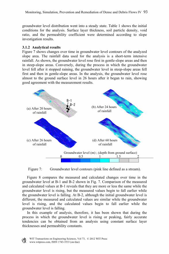
3.1.2 Analytical results Figure 7 shows changes over time in groundwater level contours of the analyzed slope area. The rainfall data used for the analysis is a short-term intensive rainfall. As shown, the groundwater level rose first in gentle-slope areas and then in steep-slope areas. Conversely, during the process in which the groundwater level fell after it stopped raining, the groundwater level in steep-slope areas fell first and then in gentle-slope areas. In the analysis, the groundwater level rose almost to the ground surface level in 26 hours after it began to rain, showing good agreement with the measurement results.

Figure 7: Groundwater level contours (pink line defined as a stream).

Figure 8 compares the measured and calculated changes over time in the groundwater level at B-1 and B-2 shown in Fig. 7. Comparison of the measured and calculated values at B-1 reveals that they are more or less the same while the groundwater level is rising, but the measured values begin to fall earlier while the groundwater level is falling. At B-2, although the initial groundwater level is different, the measured and calculated values are similar while the groundwater level is rising, and the calculated values begin to fall earlier while the groundwater level is falling. In this example of analysis, therefore, it has been shown that during the process in which the groundwater level is rising or peaking, fairly accurate tendencies can be obtained from an analysis using constant surface layer thicknesses and permeability constants.

0 0.5 1 1.5 2 Groundwater level (m) ; (depth from ground surface)

2.5

1 125

2.5

1 876

2.5

0 196

(c) After 26 hours of rainfall

(d) After 60 hours of rainfall

(b) After 24 hours of rainfall

(a) After 20 hours of rainfall

2.5

0 022

B-1 B-2



Figure 8: Relationship between rainfall and groundwater level.

3.2 Example of analysis of stability

3.2.1 Analysis conditions The analyzed slope is a slope where a debris flow occurred in the past. The analysis was carried out by using the rainfall data at the time of the debris flow; the maximum hourly rainfall is 27 mm/h and the cumulative rainfall is 199 mm. The relationships of the groundwater level with some analysis parameters, namely, soil particle density, void ratio, permeability coefficient and the degree of saturation, were determined on the basis of the results of various laboratory tests conducted by using specimens collected at the site. The surface layer thickness was determined on the basis of the results of simple dynamic cone penetration tests carried out at the site. For soil strength parameter, the values obtained by assuming an internal friction angle of 30 degrees and back-calculating the cohesion of soil so that the factor of safety for the steepest element of the slope of interest becomes 1.2 were used.

3.2.2 Analytical results Figure 9 shows stability distributions at 0 and 40 hours (cumulative rainfall 193 mm) in the analysis. As shown, the stability of the slopes near the streams has decreased because of rain. Field investigation confirmed the existence of many slope failure sites near the streams, showing that the analytical results are consistent with the site conditions. Thus, the proposed method accurately captures changing stability of the near-stream slope, which is thought to greatly affect the occurrence of debris flows. Figure 10 shows the changes in hourly rainfall and the changes in the flow rate at the outlet of the stream. This figure indicates that immediately after hourly rainfall peaks, the water flow rate at the outlet of the stream peaks. In many of the debris flows that occurred in the past, stream runoff peaked immediately after hourly rainfall peaked, and a debris flow occurred almost at the same time. This tendency, which was observed in past debris flows when debris flow risk increased, is consistent with the analytical results. From this, it can be concluded

Hou

rly

Rai

nfal

l (m

m/h

)

-2.5

-2

-1.5

-1

-0.5

0

0 20 40 60

0

50

100

150

200

計測結果

解析結果

時間雨量

0.5

1.0

1.5

2.0

2.5 Gro

undw

ater

leve

l (m

) (d

epth

fro

m g

roun

d su

rfac

e)

Time

measured calculated

Rainfall-2.5

-2

-1.5

-1

-0.5

0

0 20 40 60

0

50

100

150

200

計測結果

解析結果

時間雨量

0.5

1.0

1.5

2.0

2.5

Time

measured calculated

Rainfa

Gro

undw

ater

leve

l (m

) (d

epth

fro

m g

roun

d su

rfac

e)

Hou

rly

Rai

nfal

l (m

m/h

) B-1 B-2



Stream outlet

Stream

Slope stability

High

Low

Figure 9: Changes in risk level.

Figure 10: Changes in flow rate at stream outlet.

that the debris flow risk evaluation method using the proposed method can be used to obtain reasonable results.

4 Summary and tasks ahead

(1) A method for expressing the three-dimensional distribution of the changing groundwater level has been developed, taking into consideration rain-induced water flow in the surface layer of the slope of interest. By performing stability calculation for the slope of interest on the basis of the water level obtained by this method, changes in stability can be shown three-dimensionally, and the results thus obtained can be used for debris flow risk evaluation. (2) One characteristic of the proposed method is that streams, which are thought to greatly affect water flow in slopes, can be defined.

0

5

10

15

20

25

30

0 20 40 60 80 100

0

50

100

150

200

250

Hou

rly

rain

fall

(m

m/h

)

Flo

w r

ate

at s

trea

m o

utle

t (m

3 /h)

Analysis time (hour)

Flow rate at stream outlet

Rainfall

After 0 hours of rainfall After 40 hours of rainfall

(cumulative rainfall： 193mm)



(3) In the proposed method, the effect of soil type on the groundwater level can be expressed in analytical results by using the relationship between the groundwater level in the slope surface layer and the degree of saturation. (4) The relationship between measured values and calculated values showed differences between the groundwater level rising process and the groundwater level falling process. The cause of these differences needs to be identified by studying the calculation process in detail. (5) It is necessary to investigate the effects of changes in surface layer thickness, permeability coefficient, etc., on calculated changes and develop methods for determining the values of these parameters.

5 Concluding remarks

This paper has reported on a study conducted to develop a method for evaluating rain-induced debris flow risk and described the results of the study on the method of predicting the groundwater movement in the surface layer of the slope of interest by using a simple calculation method. As the next step, the authors will evaluate the validity and applicability of the proposed model by solving the problems mentioned in this paper and applying the method to various slopes. On the basis of the proposed method, the authors also hope to establish a method for controlling train operation during rainfall.

References

[1] Okimura, T. and Ichikawa, R., Surface failure risk prediction method using digital terrain model (in Japanese). Journal of JSCE, Vol. 358/III-3, pp. 69–75, June, 1985.

[2] Yamaguchi, H., Soil mechanics (in Japanese), pp. 55, 1984. [3] Okada, K., Iwasaki, S., Sugiyama, T. and Muraishi, H., Estimation of

steady-state groundwater level for stability analysis of fills during heavy rain (in Japanese). 34th Japan National Conference on Geotechnical Engineering, pp. 2121–2122, 1999.



Risk assessment method of debris flow occurrence utilizing ...

Documents

Transcript of Risk assessment method of debris flow occurrence utilizing ...