Risk and return: evaluating reverse tracing of precursors...

GJI gji_4666 Dispatch: June 8, 2010 CE: WRV

Journal MSP No. No. of pages: 8 PE: JM12

3456789

10111213141516171819202122232425262728293031323334353637383940414243444546474849505152535455565758596061626364

Geophys. J. Int. (2010) doi: 10.1111/j.1365-246X.2010.04666.x

GJI

Sei

smol

ogy

Risk and return: evaluating reverse tracing of precursors earthquakepredictions

Q1

Q2Q3

J. Douglas Zechar1,2 and Jiancang Zhuang3

1Swiss Seismological Service, Institute of Geophysics, ETH Zurich, Sonneggstrasse 5, 8092 Zurich, Switzerland. E-mail: [email protected] Earth Observatory, Columbia University, NY, USA3Institute of Statistical Mathematics

Accepted 2010 May 17. Received 2010 May 3; in original form 2010 February 25

S U M M A R YIn 2003, the reverse tracing of precursors (RTP) algorithm attracted the attention of seismol-ogists and international news agencies when researchers claimed two successful predictionsof large earthquakes. These researchers had begun applying RTP to seismicity in Japan,California, the eastern Mediterranean and Italy; they have since applied it to seismicity in thenorthern Pacific, Oregon and Nevada. RTP is a pattern recognition algorithm that uses earth-quake catalogue data to declare alarms, and these alarms indicate that RTP expects a moderateto large earthquake in the following months. The spatial extent of alarms is highly variableand each alarm typically lasts 9 months, although the algorithm may extend alarms in timeand space. We examined the record of alarms and outcomes since the prospective applicationof RTP began, and in this paper we report on the performance of RTP to date. To analysethese predictions, we used a recently developed approach based on a gambling score, and weused a simple reference model to estimate the prior probability of target earthquakes for eachalarm. Formally, we believe that RTP investigators did not rigorously specify the first two ‘suc-cessful’ predictions in advance of the relevant earthquakes; because this issue is contentious,we consider analyses with and without these alarms. When we included contentious alarms,RTP predictions demonstrate statistically significant skill. Under a stricter interpretation, thepredictions are marginally unsuccessful.

Key words: Probabilistic forecasting; Probability distributions; Earthquake interaction, fore-casting, and prediction; Seismicity and tectonics; Statistical seismology.

1 I N T RO D U C T I O N

In this paper, we present an analysis of earthquake predictions thatwere generated by reverse tracing of precursors (RTP), a patternrecognition algorithm intended to predict large earthquakes in atime window of at least 9 months (Keilis-Borok et al. 2004; Shebalinet al. 2004, 2006). Below, we provide a conceptual overview of RTPwith an emphasis on the details relevant to this study, and we referthe interested reader to Section 2 and Table 3 of Shebalin et al.(2004) for a comprehensive description of the algorithm.

RTP searches for seismicity precursors in two distinct steps:short-term recognition and intermediate-term confirmation. In thefirst step, the algorithm decomposes a declustered regional earth-quake catalogue into chains, which are composed of neighbours(Shebalin 2006); two earthquakes are neighbours if they occur suffi-ciently close in space and time, where the definition of ‘sufficientlyclose’ depends on the magnitudes of the two earthquakes. Aftergrouping all earthquakes into chains, RTP keeps only the chainsthat have a large spatial extent and comprise several events. Thealgorithm interprets chains that satisfy these criteria as signals of

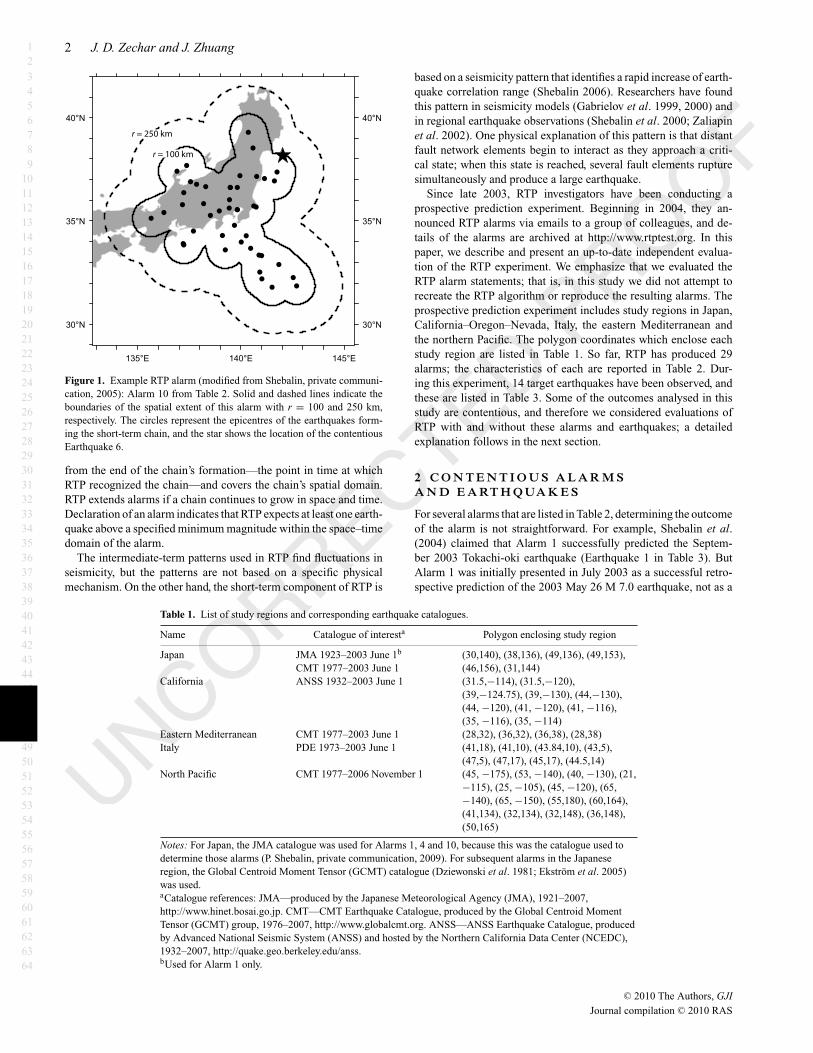
a short-term precursor to a target earthquake. A chain’s spatial do-main is delimited by the union of circles of radius r that are centredon each epicentre in the chain and the area connecting these circles.See Fig. 1 for an example of a chain’s spatial extent with varying r.

The second step of RTP seeks to confirm (or disconfirm) theshort-term precursor by searching for intermediate-term patternswithin each precursory chain’s spatial domain. In this step, valuesof eight precursory functions (described in Table 2 of Shebalin et al.2004) are computed. These functions capture four types of supposedprecursory behaviour: increased seismic activity, increased spatialclustering, increased correlation length and a transformed relation-ship between earthquake frequency and magnitude. Researchershave used such precursory behaviours in previous prediction stud-ies with some limited success (see reviews by Keilis-Borok 2002,2003).

The algorithm computes the values of the intermediate-term pre-cursory functions in sliding time windows, and it defines thresholdvalues for each combination of precursory function and window-ing value, yielding 64 threshold values. If many of these thresholdvalues are exceeded, RTP declares an alarm that lasts for 9 months

C© 2010 The Authors 1Journal compilation C© 2010 RAS

12

3456789

10111213141516171819202122232425262728293031323334353637383940414243444546474849505152535455565758596061626364

2 J. D. Zechar and J. Zhuang

Figure 1. Example RTP alarm (modified from Shebalin, private communi-cation, 2005): Alarm 10 from Table 2. Solid and dashed lines indicate theboundaries of the spatial extent of this alarm with r = 100 and 250 km,respectively. The circles represent the epicentres of the earthquakes form-ing the short-term chain, and the star shows the location of the contentiousEarthquake 6.

from the end of the chain’s formation—the point in time at whichRTP recognized the chain—and covers the chain’s spatial domain.RTP extends alarms if a chain continues to grow in space and time.Declaration of an alarm indicates that RTP expects at least one earth-quake above a specified minimum magnitude within the space–timedomain of the alarm.

The intermediate-term patterns used in RTP find fluctuations inseismicity, but the patterns are not based on a specific physicalmechanism. On the other hand, the short-term component of RTP is

based on a seismicity pattern that identifies a rapid increase of earth-quake correlation range (Shebalin 2006). Researchers have foundthis pattern in seismicity models (Gabrielov et al. 1999, 2000) andin regional earthquake observations (Shebalin et al. 2000; Zaliapinet al. 2002). One physical explanation of this pattern is that distantfault network elements begin to interact as they approach a criti-cal state; when this state is reached, several fault elements rupturesimultaneously and produce a large earthquake.

Since late 2003, RTP investigators have been conducting aprospective prediction experiment. Beginning in 2004, they an-nounced RTP alarms via emails to a group of colleagues, and de-tails of the alarms are archived at http://www.rtptest.org. In thispaper, we describe and present an up-to-date independent evalua-tion of the RTP experiment. We emphasize that we evaluated theRTP alarm statements; that is, in this study we did not attempt torecreate the RTP algorithm or reproduce the resulting alarms. Theprospective prediction experiment includes study regions in Japan,California–Oregon–Nevada, Italy, the eastern Mediterranean andthe northern Pacific. The polygon coordinates which enclose eachstudy region are listed in Table 1. So far, RTP has produced 29alarms; the characteristics of each are reported in Table 2. Dur-ing this experiment, 14 target earthquakes have been observed, andthese are listed in Table 3. Some of the outcomes analysed in thisstudy are contentious, and therefore we considered evaluations ofRTP with and without these alarms and earthquakes; a detailedexplanation follows in the next section.

2 C O N T E N T I O U S A L A R M SA N D E A RT H Q UA K E S

For several alarms that are listed in Table 2, determining the outcomeof the alarm is not straightforward. For example, Shebalin et al.(2004) claimed that Alarm 1 successfully predicted the Septem-ber 2003 Tokachi-oki earthquake (Earthquake 1 in Table 3). ButAlarm 1 was initially presented in July 2003 as a successful retro-spective prediction of the 2003 May 26 M 7.0 earthquake, not as a

Table 1. List of study regions and corresponding earthquake catalogues.

Name Catalogue of interesta Polygon enclosing study region

Japan JMA 1923–2003 June 1b

CMT 1977–2003 June 1(30,140), (38,136), (49,136), (49,153),(46,156), (31,144)

California ANSS 1932–2003 June 1 (31.5,−114), (31.5,−120),(39,−124.75), (39,−130), (44,−130),(44, −120), (41, −120), (41, −116),(35, −116), (35, −114)

Eastern Mediterranean CMT 1977–2003 June 1 (28,32), (36,32), (36,38), (28,38)Italy PDE 1973–2003 June 1 (41,18), (41,10), (43.84,10), (43,5),

(47,5), (47,17), (45,17), (44.5,14)North Pacific CMT 1977–2006 November 1 (45, −175), (53, −140), (40, −130), (21,

−115), (25, −105), (45, −120), (65,−140), (65, −150), (55,180), (60,164),(41,134), (32,134), (32,148), (36,148),(50,165)

Notes: For Japan, the JMA catalogue was used for Alarms 1, 4 and 10, because this was the catalogue used todetermine those alarms (P. Shebalin, private communication, 2009). For subsequent alarms in the Japaneseregion, the Global Centroid Moment Tensor (GCMT) catalogue (Dziewonski et al. 1981; Ekstrom et al. 2005)was used.aCatalogue references: JMA—produced by the Japanese Meteorological Agency (JMA), 1921–2007,http://www.hinet.bosai.go.jp. CMT—CMT Earthquake Catalogue, produced by the Global Centroid MomentTensor (GCMT) group, 1976–2007, http://www.globalcmt.org. ANSS—ANSS Earthquake Catalogue, producedby Advanced National Seismic System (ANSS) and hosted by the Northern California Data Center (NCEDC),1932–2007, http://quake.geo.berkeley.edu/anss.bUsed for Alarm 1 only.

C© 2010 The Authors, GJI

Journal compilation C© 2010 RAS

12

3456789

10111213141516171819202122232425262728293031323334353637383940414243444546474849505152535455565758596061626364

Evaluating RTP predictions 3

Table 2. List of all announced RTP alarms, including the study region, time range of interest, target magnitude range and alarm radius.

Alarm no., i Region Alarm start Alarm end Magnitude Radius, r (km)

1a Japan 2003 March 27 2003 November 27 M JMA ≥ 7.0 752a California 2003 May 5 2004 February 27 MANSS ≥ 6.4 753 California 2003 November 13 2004 September 5 MANSS ≥ 6.4 504 Japan 2004 February 8 2004 November 8 Mw ≥ 7.2 1005a Italy 2004 February 29 2004 November 29 Mw ≥ 5.5 506 California 2004 November 14 2005 August 14 MANSS ≥ 6.4 507 California 2004 November 16 2005 August 16 MANSS ≥ 6.4 508 Italy 2004 December 31 2005 October 1 MPDE ≥ 5.5 509 Italy 2005 May 6 2006 February 6 MPDE ≥ 5.5 5010a Japan 2005 June 2 2006 March 2 Mw ≥ 7.2 10011 California 2005 June 17 2006 March 17 MANSS ≥ 6.4 5012 California 2006 March 18 2006 September 18 MANSS ≥ 6.4 5013 California 2006 March 24 2006 December 24 MANSS ≥ 6.4 5014 California 2006 December 25 2007 May 2 MANSS ≥ 6.4 5015 Italy 2006 May 2 2007 February 3 MPDE ≥ 5.5 10016 Japan 2006 May 11 2007 February 11 Mw ≥ 7.2 10017 California 2006 September 23 2007 June 23 MANSS ≥ 6.4 5018 Japan 2006 September 30 2007 June 30 Mw ≥ 7.2 10019 North Pacific 2006 October 28 2007 July 28 Mw ≥7.2 10020 California 2007 January 17 2007 October 17 MANSS ≥ 6.4 5021 California 2007 May 3 2008 January 28 MANSS ≥ 6.4 5022 California 2007 October 18 2008 January 14 MANSS ≥ 6.4 5023 North Pacific 2007 July 29 2008 January 28 Mw ≥ 7.2 10024 North Pacific 2007 August 24 2008 May 24 Mw ≥ 7.2 10025 California 2008 January 29 2008 September 26 MANSS ≥ 6.4 5026 Italy 2008 April 7 2009 January 7 MPDE ≥ 5.5 5027 California 2008 April 14 2009 January 14 MANSS ≥ 6.4 5028 North Pacific 2008 July 17 2009 April 17 Mw ≥ 7.2 10029 California 2009 January 29 2009 October 29 MANSS ≥ 6.4 50

Note: Alarms are listed in chronological order according to their start date. The epicentres that define the spatial extent of each alarm regionare listed in Supporting Information.aContentious alarm; see Section 2 for details.

Table 3. Earthquakes with magnitudes that equal or exceed the typical target magnitude for the RTP study region in which they occurred,having occurred since testing began in the respective region.

Earthquake no. Region Origin date Magnitude Latitude (◦) Longitude (◦) Inside alarm?

1a Japan 2003 September 25 M JMA = 8.0 42.21 143.84 Maybe2a Japan 2003 September 25 Mw = 7.3 41.75 143.62 Maybe3a California 2003 December 22 MANSS = 6.5 35.70 −121.10 Maybe4 California 2005 June 15 MANSS = 7.2 41.29 −125.95 No5 California 2005 June 17 MANSS = 6.6 40.77 −126.57 No6a Japan 2005 August 16 Mw = 7.2 38.24 142.05 Maybe7 Japan 2006 November 15 Mw = 8.3 46.71 154.33 Yes8 Japan 2007 January 13 Mw = 8.1 46.17 154.80 Yes9 North Pacific 2007 December 19 Mw = 7.2 51.02 −179.27 Yes10 North Pacific 2008 July 5 Mw = 7.7 54.12 153.37 No11 North Pacific 2008 November 24 Mw = 7.3 54.27 154.71 No12 North Pacific 2009 January 15 Mw = 7.4 46.97 155.39 No13 Italy 2009 April 6 Mw = 6.3 42.33 13.33 No14 Italy 2009 April 7 Mw = 5.5 42.28 13.46 No

Note: Events with magnitudes listed as Mw are listed as reported from the GCMT catalogue.aContentious earthquake; see Section 2 for details.

prospective prediction (Shebalin et al. 2003). In addition, Shebalinet al. (2003) did not include the magnitude range of interest or thealarm duration in the alarm description. One could argue that themagnitude range could be inferred from the fact that the 2003 May26 event was considered a target earthquake, but the alarm durationwas not specified. Therefore, it is contentious to interpret alarm 1as a successful prediction of Earthquakes 1 and 2.

Similarly, RTP investigators declared Alarm 2 in a memo sentto colleagues, and the memo included neither an explicit statement

of the alarm time window nor a definition of the target earthquake;rather, the authors used vague phrases such as ‘preparing for a majorearthquake’ (K. Aki et al. private communication, 2003). Therefore,it is suspect to interpret alarm 2 as a successful prediction of the2003 San Simeon earthquake (Earthquake 3).

For Alarm 5 in Italy, RTP investigators announced the targetmagnitude range as Mw ≥ 5.5, although they had developed andoptimized RTP using the ‘official magnitude’ of the PDE catalogue(P. Shebalin, private communication, 2009). If the PDE catalogue



12

3456789

10111213141516171819202122232425262728293031323334353637383940414243444546474849505152535455565758596061626364


contains more than one estimate of magnitude for an earthquake,the official magnitude is the maximum of all estimates. An eventwith ML 5.7 occurred within the space–time extent of Alarm 5,but, because the reported moment magnitude was Mw 5.2, Alarm 5formally cannot be considered successful.

Because of a delay in the earthquake catalogue data used tosearch for chains in the Japan testing region, RTP investigators didnot declare Alarm 10 until after Earthquake 6 occurred (P. Shebalinprivate communication, 2009). If they had declared this alarm inadvance of the earthquake, it would be a clear success; yet given thecircumstances, the success of Alarm 10 as a prospective predictionof Earthquake 6 is questionable.

Because these alarms are contentious, we present two evalua-tions: one that includes these alarms and the corresponding targetearthquakes, and another that excludes them. We refer to theseevaluations as the loose interpretation and the strict interpretation,respectively.

3 E VA LUAT I O N M E T H O D S

In the context of deterministic prediction of binary events, there arefour possible outcomes: If one predicts that an event will happen (apositive prediction) and it happens, this is a hit. If one predicts thatan event will happen but it does not happen, this is a false alarm.If one predicts that an event will not happen (a negative prediction)but it does happen, this is a miss. If one predicts that an event willnot happen and it does not happen, this is a correct negative.

To measure the skill of a set of predictions, one can organizethe outcomes in a contingency table, which denotes the frequencyof each outcome, and choose some related metric to quantify skill(Mason 2003). In the specific context of deterministic earthquakeprediction, one such metric that has been used is the R-score (alsoknown as the Hanssen–Kuiper skill score) (Shi et al. 2001; Harte &Vere-Jones 2005). The R-score is defined as the difference betweenthe hit rate and the false alarm rate

R = a

a + c− b

b + d, (1)

where a is the number of hits, b is the number of false alarms, cis the number of misses and d is the number of correct negatives.The R-score of RTP is uninformative because RTP only producespositive predictions; therefore, c and d are zero and, regardless ofthe alarms and outcomes, R is always zero. Wherever there is noRTP alarm in space and time, we interpreted this as a statementof no prediction rather than inferring a negative prediction; wediscuss the alternative interpretation in Section 6. We note thatmost contingency table metrics, including the R-score, implicitlyassume that the probability of a hit is the same for each prediction;this is not the case for RTP alarms (details in Section 4), and it israrely the case for earthquake predictions in general.

Another diagnostic that is commonly used to evaluate the per-formance of alarm-based earthquake predictions is the Molchandiagram (Molchan & Keilis-Borok 2008; Zechar & Jordan 2008),which compares the fraction of space–time–magnitude covered byalarms with the miss rate, ν = c/(a + c). Unfortunately, because RTPdoes not issue negative alarms, the miss rate of RTP is always zero,and therefore the Molchan diagram approach is also uninformative.

Because the usual contingency table measures are not informa-tive for RTP, we used the gambling score of Zhuang (2010). Thisscoring approach requires the explicit choice of a reference modelfor earthquake probability; the Poisson process is a reasonable ref-

Q4 erence model for ‘independent’ events (Gardner & Knopoff 1974),

and the Omori–Utsu distribution (Utsu et al. 1995) is appropriate forevaluating ‘aftershock’ forecasts. For evaluation of RTP alarms, thePoisson reference model yields prior probabilities for the successof each alarm.

To understand the gambling score method, suppose that the ref-erence model indicates a probability p that at least one target earth-quake will occur in a given space–time–magnitude window. Thinkof the forecaster as a gambler and a prediction as being a bet ofone credit of professional reputation. RTP does not yield negativepredictions, so one only needs to consider positive predictions. (Werefer the reader to Zhuang (2010) for details on negative predictionsand an extension to probabilistic forecasts.) The RTP forecaster canbet one reputation credit on ‘Yes’, or he may abstain from bettingif no RTP prediction is available. If no target earthquake satisfiesthe alarm, the forecaster loses and his reputation is diminished byone credit. If at least one target earthquake satisfies the alarm, hecorrectly bet on ‘Yes’ and he gains credits according to the returnratio for ‘Yes’ bets, rYES = (1 − p)/p. This ratio is designed suchthat the expected change in reputation, �R, for this bet is zero ifthe reference model is an exact representation of the system (i.e. itis the ‘true’ model)

E[�R] = rYES p − (1 − p) = 0, (2)

where E[x] denotes the expectation of x. Zhuang (2010) proved thatif a set of predictions obtains a positive �R, the prediction model issuperior to the reference model; in particular, a gain in reputationindicates that the correlation between the prediction model and the(unknown) true model is greater than the correlation between thereference model and the true model.

4 R E F E R E N C E P RO B A B I L I T YA NA LY S I S

The gambling score method requires the explicit choice of a ref-erence model with which to compare a forecaster’s bets. Con-sidering alarm-based predictions, the reference model yields anestimate of the probability that an alarm will be successful or,equivalently, the probability that at least one earthquake will occurin the space–time–magnitude domain of an alarm. Assuming thattarget earthquake rates are well described by a Poisson process, thereference model needs to estimate only the probability of at leastone earthquake occurring in the space–duration–magnitude domainof an alarm, without regard for the specific time period of the alarm.In other words, if the alarm duration is 9 months, the Poisson ref-erence probability is relevant to any 9-month period covering thesame space–magnitude domain, not only the9-month period duringwhich the alarm is active. Although there is ample evidence that thePoisson distribution is less than ideal for describing earthquake ratevariability (Kagan 2010; Schorlemmer et al. 2010), we neverthelessused a Poisson reference model because of its uniform applicabil-ity to all alarms and because of its simplicity—namely, it includesfew assumptions and it is easily interpreted. To estimate the refer-ence probability for the ith alarm Ai, we used the relevant catalogue(Table 1) and computed the daily rate of earthquakes, N(mi), in Ai’sspace–magnitude domain. When estimating this rate, we includedall events that occurred before the alarm was declared. Under thePoisson assumption, the probability of observing at least one earth-quake in the space–magnitude domain of Ai in a time window ofduration ti days is

pi = 1 − exp(−N (mi )ti ). (3)



12

3456789

10111213141516171819202122232425262728293031323334353637383940414243444546474849505152535455565758596061626364


Table 4. Duration ti, minimum magnitude mi, historical daily rate, N(mi)or N(mi), and corresponding Poisson reference probability pi (from eq. 3)for each alarm.

Alarm no., i ti (days) mi N(mi) N(mi) pi (%)

1 246 7.2 1.40E−4 – 29.122 299 6.4 7.68E−5 – 2.273 308 6.4 3.05E−4 – 8.964 275 7.2 1.01E−4 – 2.745 275 5.5 7.03E−4 – 17.586 274 6.4 1.50E−4 – 4.037 274 6.4 – 1.01E−4 2.748 275 5.5 5.13E−4 – 13.179 277 5.5 7.62E−4 – 19.0310 274 7.2 9.63E−5 – 2.6111 274 6.4 2.61E−4 – 6.9012 185 6.4 1.11E−4 – 2.0313 276 6.4 3.32E−4 – 8.7614 129 6.4 2.92E−4 – 3.7015 278 5.5 8.21E−4 – 20.4216 277 7.2 9.33E−4 – 22.7717 274 6.4 – 7.33E−5 1.9918 274 7.2 6.44E−4 – 16.1819 274 7.2 3.67E−4 – 9.5720 274 6.4 1.09E−4 – 2.9521 271 6.4 2.54E−4 – 6.6622 89 6.4 1.08E−4 – 0.9623 184 7.2 3.58E−4 – 6.3824 275 7.2 – 4.47E−5 1.2225 242 6.4 2.52E−4 – 5.9126 276 5.5 1.55E−4 – 4.2027 276 6.4 – 1.04E−4 2.8328 275 7.2 – 3.58E−6∗ 0.9829 274 6.4 7.10E−5 – 1.93

Note: When the historical rate N(mi) was zero, we used the rate of smallerevents N(mi) ∼ N(mi – �m) to estimate the alarm’s success probability. IfN(mi) was zero, we arbitrarily set the rate to one-half earthquake per theduration of the catalogue; this is marked with an asterisk.

For any alarm where N(mi) = 0—that is, the catalogue containedno earthquakes with magnitude at least mi in the alarm’s geo-graphic domain—we estimated the rate of target earthquakes usingN(mi − �m), a rate that includes smaller events. We did this be-cause earthquake catalogues are finite and a zero rate/probabilityseems unphysical. In estimating this rate of target earthquakes, wefurther assumed that the magnitude–frequency distribution followsthe Gutenberg–Richter relation with a b-value of unity

N (mi ) = N (mi − �m)

10�m. (4)

For alarms where N(mi) = 0, we chose �m = 1 and substitutedthe estimate N(mi) of eq. 4 for N(mi) in eq. 3. For Alarm 28, eventhis estimation yielded a zero rate. For this special situation, wearbitrarily set the rate to one earthquake per twice the durationof the catalogue. This choice corresponds to a posterior estimatein which the rate has a prior density that is proportional to thelikelihood.

For each alarm, we report in Table 4 the minimum magnitudeof interest, duration, estimated daily rate of earthquakes and corre-sponding prior probability. The probabilities represent the chanceof each alarm’s success under the Poisson reference model, and theyvary widely from alarm to alarm. As mentioned in the previous sec-tion, this variation makes the application of most contingency tablemeasures invalid.

We emphasize that the reference probabilities for false alarmsare not used for the RTP gambling score calculation and we report

them here to be consistent and to facilitate comparison of alarms.Therefore, our most uncertain estimates (for Alarm 28 and all othersbased on eq. 4) do not affect the gambling score results.

5 R E S U LT S

In Table 5, we report the results of testing the RTP alarms withthe gambling score and a Poisson reference model. Because someof the outcomes are contentious, we present results from two end-member interpretations. The loose interpretation counts the con-tentious alarms as successful predictions, whereas the strict inter-pretation ignores the contentious alarms or, for Alarm 5, countsthem as false alarms. The total return from the 29 RTP alarms is84.4 credits under the loose interpretation and −4.15 credits underthe strict interpretation. Because the former value is positive, underthe loose interpretation the gambling score deems RTP alarms su-perior to the Poisson reference model. On the other hand, the strictinterpretation result indicates performance that is marginally worsethan the Poisson model. The biggest difference between the resultsis caused by the reputation credits associated with Alarm 2 andthe 2003 San Simeon earthquake (Earthquake 3), which occurredin a region of relatively low historical seismic activity. Neglectingthis earthquake and the corresponding alarm (as we did under thestrict interpretation), the total reputation gain is negative. The othermajor contribution to the reputation gain is Alarm 23 (Earthquake9), which resulted in a 14.7 credit increase.

The gambling score approach allows a straightforward hypothesistest regarding the RTP alarms. In the context of this study, the nullhypothesis is that the performance of the RTP alarms, quantifiedby the net gambling score return, is no better than what could beexpected from the Poisson reference model. In other words, we areinterested in the question: is the RTP reputation change significantlylarger than what one would obtain if bets were placed according tothe reference probabilities? To address this question, we used a sim-ple simulation method. For each RTP alarm, a number was chosenrandomly from the uniform distribution on [0, 1). If the selectednumber was smaller than the reference probability for the RTPalarm, an identical, positive alarm was declared; if the number waslarger, a negative alarm covering the same space–time–magnitudevolume was declared. After this process was repeated for all RTPalarms, a gambling score was computed for this set of simulatedalarms {Xi}

�R =∑

i

[Xi Yi

(1 − pi

pi

)+ (1 − Xi ) Yi (−1)

+ Xi (1 − Yi ) (−1) + (1 − Xi ) (1 − Yi )

(pi

1 − pi

) ]. (5)

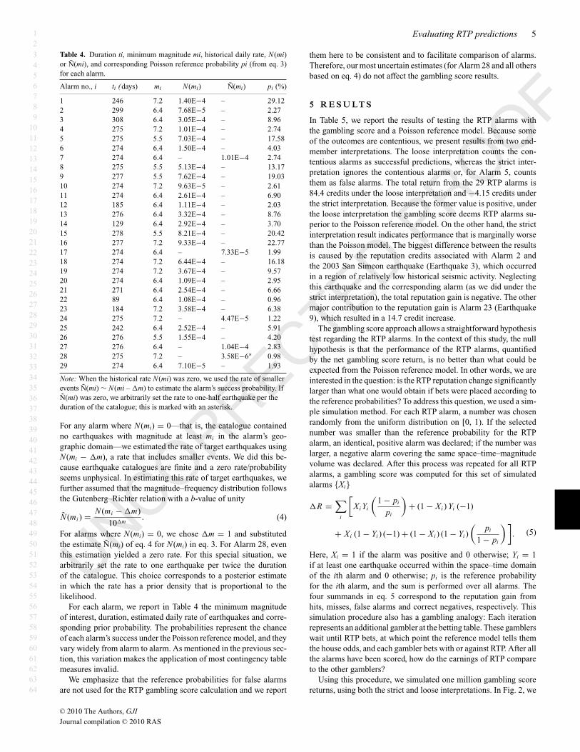
Here, Xi = 1 if the alarm was positive and 0 otherwise; Yi = 1if at least one earthquake occurred within the space–time domainof the ith alarm and 0 otherwise; pi is the reference probabilityfor the ith alarm, and the sum is performed over all alarms. Thefour summands in eq. 5 correspond to the reputation gain fromhits, misses, false alarms and correct negatives, respectively. Thissimulation procedure also has a gambling analogy: Each iterationrepresents an additional gambler at the betting table. These gamblerswait until RTP bets, at which point the reference model tells themthe house odds, and each gambler bets with or against RTP. After allthe alarms have been scored, how do the earnings of RTP compareto the other gamblers?

Using this procedure, we simulated one million gambling scorereturns, using both the strict and loose interpretations. In Fig. 2, we



12

3456789

10111213141516171819202122232425262728293031323334353637383940414243444546474849505152535455565758596061626364


Table 5. Success probability, loose and strict interpretations of the outcome, and corresponding changes in repu-tation for each alarm.

Alarm no., i Success probability, pi (%) Outcome (loose) Outcome (strict) �Ri (loose) �Ri (strict)

1 29.12 Hita (Eqk. 1, 2) – 2.43 –2 2.27 Hitb (Eqk. 3) – 43.07 –3 8.96 False alarm False alarm −1.00 −1.004 2.74 False alarm False alarm −1.00 −1.005 17.58 Hitc False alarm 4.69 −1.006 4.03 False alarm False alarm −1.00 −1.007 2.74 False alarm False alarm −1.00 −1.008 13.17 False alarm False alarm −1.00 −1.009 19.03 False alarm False alarm −1.00 −1.0010 2.61 Hitd (Eqk. 6) – 37.38 –11 6.90 False alarm False alarm −1.00 −1.0012 2.03 False alarm False alarm −1.00 −1.0013 8.76 False alarm False alarm −1.00 −1.0014 3.70 False alarm False alarm −1.00 −1.0015 20.42 False alarm False alarm −1.00 −1.0016 22.77 False alarm False alarm −1.00 −1.0017 1.99 False alarm False alarm −1.00 −1.0018 16.18 Hit (Eqk. 7, 8) Hit (Eqk. 7, 8) 5.18 5.1819 9.57 False alarm False alarm −1.00 −1.0020 2.95 False alarm False alarm −1.00 −1.0021 6.66 False alarm False alarm −1.00 −1.0022 0.96 False alarm False alarm −1.00 −1.0023 6.38 Hit (Eqk. 9) Hit (Eqk. 9) 14.67 14.6724 1.22 False alarm False alarm −1.00 −1.0025 5.91 False alarm False alarm −1.00 −1.0026 4.20 False alarm False alarm −1.00 −1.0027 2.83 False alarm False alarm −1.00 −1.0028 0.98 False alarm False alarm −1.00 −1.0029 1.93 False alarm False alarm −1.00 −1.00Total reputation change 84.42 −4.15

Note: For those outcomes interpreted as hits, we also note the earthquake number (from Table 3), which the alarmhas been interpreted to predict.aThe magnitude range was not specified in advance of the target earthquake; see Section 2 for details.bThe magnitude range was not specified in advance of the target earthquake; see Section 2 for details.cMagnitude ambiguously specified in original alarm statement; see Section 2 for details.dDue to delay of catalogue data, the alarm was declared after a satisfactory target earthquake; see Section 2 fordetails.

show the resulting empirical cumulative distribution functions foreach set of simulated gambling scores. Under the loose interpreta-tion, the null hypothesis is rejected with a high level of confidence:less than 0.009% of all simulations resulted in a reputation gainof more than 84.4 credits. But under the strict interpretation, theresult is decidedly less compelling, and the null hypothesis cannotbe rejected with much confidence: nearly 93.70% of the simulationshad reputation gains larger than the 4.15 credits lost by RTP.

6 D I S C U S S I O N A N D C O N C LU S I O N S

Using a Poisson reference model and the gambling score methodof Zhuang (2010), we evaluated the 29 prospective earthquake pre-diction alarms produced by RTP investigators. Because the detailsof several of the alarms and the corresponding outcomes are debat-able, we considered a very formal, strict interpretation of the alarmsusing the exact statements of the RTP investigators. To be fair, wealso considered a very loose interpretation that favoured RTP in anydoubtful situation. When using the loose interpretation, we foundthat RTP was significantly better than a simple Poisson referencemodel, mostly due to the prediction involving the 2003 San Simeonearthquake. When using the strict interpretation, because the 2003

San Simeon earthquake and the related alarm were disregarded, thenull hypothesis that RTP is no better than a Poisson model could notbe rejected with much confidence; indeed, RTP fared marginallyworse than the Poisson model.

At least one aspect of this study may be discomfiting to the reader:because RTP declared only positive alarms, it is not penalized for theoccurrence of those large earthquakes inside RTP study regions andoutside any alarm (Earthquakes 4, 5, 10–14 in Table 3)—outcomesthat normally might be considered misses. Nevertheless, RTP didnot issue negative alarms and therefore we treated these events ashappening in regions of space–time–magnitude where no RTP betwas placed; we contend that this interpretation is the most judicious.

Alternatively, what if one treated any lack of an alarm as a neg-ative prediction, rather than as a statement of ‘no available predic-tion’? Because this is a dubious interpretation—if not an outrightmisinterpretation—of a predictive non-statement, any evaluationthat resulted from this approach would be far from defensible. Be-yond this important semantic issue, several technical challengeswould remain: How would one estimate the reference probabilityfor a missed earthquake (as opposed to the reference probabilityfor a well-defined space–time–magnitude volume, as we used inthis study)? Could one fairly and reasonably define an appropriatevolume after a large earthquake happened? More generally, how



12

3456789

10111213141516171819202122232425262728293031323334353637383940414243444546474849505152535455565758596061626364


0

0.1

0.2

0.3

0.4

0.5

0.6

0.7

0.8

0.9

1

change in reputation

fraction o

f sim

ula

tions

0 20 40 60 80

Figure 2. Empirical cumulative distribution functions for simulated gam-bling returns under the strict interpretation (solid line) and loose interpreta-tion (dashed line). RTP reputation changes are indicated by a circle (strictinterpretation) and a square (loose interpretation). Because almost no simu-lations under the loose interpretation yield a return that is greater than RTP’sgain, the null hypothesis is rejected with great confidence—one can say thatthe RTP alarms are superior to the reference model. On the other hand, un-der the strict interpretation, because a substantial percentage of simulationshave a larger reputation increase than RTP, the null hypothesis cannot berejected with great confidence.

would the volume of each inferred negative alarm be defined, so asto also count correct negatives? If one discretized the total avail-able space–time–magnitude volume in any or all dimensions, thechoice of discretization size would affect the scoring results. Be-cause there are so many pitfalls with the alternatives, we argue thatthe interpretations used and the evaluation presented in this studyinvolve the fewest assumptions and yield the most robust results,despite effectively ignoring some of the large earthquakes listed inTable 3.

As mentioned in the Introduction, one of the RTP parametersis the radius, r, of circles centred on each event in the chain; thisparameter is used to define the spatial extent of each alarm. In thisstudy, we only considered the alarms defined by the smaller r-valuefor each alarm, consistent with the value specified for the earlyRTP alarms. Later in the experiment, RTP investigators introducedalarms based on a larger r; they announced these alarms simultane-ously with the smaller alarms (P. Shebalin private communication,2009); we chose to test only the smaller alarms. Nevertheless, forthe alarms analysed in this study, the larger alarm variants wouldfare no better than their smaller counterparts. In particular, the ref-erence probabilities would be at least as large as those reported inTable 4, and no target earthquake occurred in the larger alarms thatdid not fall within the smaller alarms; therefore, the total changesin reputation necessarily would be no greater than those reportedin Table 5. Along these same lines, we emphasize that we testedthe RTP alarm statements, not the entire algorithm as it has beendescribed in various publications. In particular, we did not declusterthe catalogues when determining target earthquakes and we did notdisregard deep events.

There are some general lessons to be learned from the contentiousalarms and earthquakes discussed in Section 2. When making earth-quake forecast statements, it is critically important that every pre-diction is well defined and unambiguously falsifiable. In the contextof RTP, the fact that the San Simeon alarm (Alarm 2) is contro-versial obscures the distinction between a result that demonstratescompelling predictive skill (under the loose interpretation) and onethat does not (under the strict interpretation). As earthquake mod-ellers increasingly rely on computer codes to analyse data and toproduce forecasts, an open-source, hands-off approach is beneficialto the forecaster’s credibility. If the RTP codes were fully auto-mated, or at least made available and documented well enough toallow reproducibility, the integrity of the forecasts would increase.

Testing the RTP alarms is not straightforward: owing to the ir-regularity with which they are announced and because there are noexplicit negative alarms, many commonly used evaluation tech-niques are not informative. More generally, we are unaware ofany other models making predictions in the same format, mannerand study regions that RTP does, and this precludes comparisonswith other earthquake prediction algorithms. The simultaneous,multiple-investigator experiments occurring within the Collabo-ratory for the Study of Earthquake Predictability (CSEP) testingcentres (Jordan 2006; Zechar et al. 2009) offer a unique oppor-tunity to advance earthquake forecasting research, and includingthe RTP algorithm in CSEP experiments might be enlightening.The investigators of RTP have attempted to share and archive theirprospective earthquake alarms. Nevertheless, it remains difficult toreproduce the algorithm by following only the publications that de-scribe the RTP approach and the outcomes of its alarms. It is alsodifficult to judge if the RTP algorithm or any of the myriad modelparameter values have changed, or are changing, as the experimentprogresses—such changes would make RTP a moving target forevaluation. Moreover, in this study we applied a testing procedurethat was designed after the experiment began, and certainly it is notthe only evaluation possible.

CSEP is designed to address these specific problems: testing cen-tres curate and execute model codes in an automated, reproducibleenvironment where the testing metrics are defined in advance (e.g.Schorlemmer et al. 2007; Zechar et al. 2010); and during prospec-tive prediction experiments, codes and model parameter values can-not be changed (Schorlemmer & Gerstenberger 2007; Zechar et al.2009). Integrating RTP into a CSEP testing centre would reducecontroversy and ambiguity related to alarm declaration and evalua-tion. The chains, alarms and the results of any test would be formallyreproducible. This would obviate the need for multiple analyses ofthe same set of alarms and further clarify whether RTP demonstratesgenuine predictive skill.

A C K N OW L E D G E M E N T S

The authors thank Peter Shebalin for his cooperation and livelyexchanges. The authors thank Christine Smyth and Patricia S. Elziefor carefully reading, and thoughtfully responding to, an early draftof the paper. The authors thank two anonymous reviewers for theirconstructive comments.

R E F E R E N C E S

Dziewonski, A.M., Chou, T.-A. & Woodhouse, J.H., 1981. Determination ofearthquake source parameters from waveform data for studies of globaland regional seismicity, J. geophys. Res., 86, 2825–2852.



12

3456789

10111213141516171819202122232425262728293031323334353637383940414243444546474849505152535455565758596061626364


Ekstrom, G., Dziewonski, A.M., Maternovskaya, N.N. & Nettles, M., 2005.Global seismicity of 2003: centroid-moment-tensor solutions for 1087earthquakes, Phys. Earth planet. Inter., 148, 327–351.

Gabrielov, A., Newman, W.I. & Turcotte, D.L., 1999. An exactly soluble hi-erarchical clustering model: inverse cascades, self-similarity and scaling,Phys. Rev. E, 60, 5293–5300.

Gabrielov, A., Keilis-Borok, V., Zaliapin, I. & Newman, W.I., 2000. Criticaltransitions in colliding cascades, Phys. Rev. E, 62, 237–249.

Harte, D. & Vere-Jones, D., 2005. The entropy score and its uses in earth-quake forecasting, Pure appl. Geophys., 162, 1229–1253.

Jordan, T.H., 2006. Earthquake predictability, brick by brick, Seism. Res.Lett., 77, 3–6.

Kagan, Y.Y., 2010. Statistical distributions of earthquake numbers: conse-quence of branching process, Geophys. J. Int., 180, 1313–1328.

Keilis-Borok, V.I., 2002. Earthquake prediction, state-of-the-art and emerg-ing possibilities, Annu. Rev. Earth planet. Sci., 30, 1–33.

Keilis-Borok, V.I., 2003. Fundamentals of earthquake prediction: fourparadigms, in Nonlinear Dynamics of the Lithosphere and EarthquakePrediction, pp. 1–36, eds Keilis-Borok, V.I. & Soloviev, A.A., Springer-Verlag, Berlin.

Keilis-Borok, V.I., Shebalin, P.N., Gabrielov, A. & Turcotte, D.L., 2004.Reverse tracing of short-term earthquake precursors, Phys. Earth planet.Inter., 145, 75–85.

Mason, I.B., 2003. Binary events, in Forecast Verification, pp. 37–76, edsJolliffe, I.T. & Stephenson, D.B., Wiley, Hoboken.

Molchan, G.M. & Keilis-Borok, V.I., 2008. Earthquake prediction: proba-bilistic aspect., Geophys. J. Int., 173, 1012–1017.

Schorlemmer, D. & Gerstenberger, M.C., 2007. RELM testing centre, Seism.Res. Lett., 78, 30–36.

Schorlemmer, D., Gerstenberger, M.C., Wiemer, S., Jackson, D.D. &Rhoades, D.A., 2007. Earthquake likelihood model testing, Seism. Res.Lett., 78(1), 17–29.

Schorlemmer, D., Zechar, J.D., Werner, M.J., Field, E.H., Jackson, D.D. &Jordan, T.H., 2010. First results of the Regional Earthquake LikelihoodModels experiment, Pure appl. Geophys., 167, 8/9, doi: 10.1007/s00024-010-0081-5.

Shebalin, P., 2006. Increased correlation range of seismicity before largeevents manifested by earthquake chains, Tectonophysics, 424, 335–349.

Shebalin, P.N., Zaliapin, I. & Keilis-Borok, V.I., 2000. Premonitory rise ofthe earthquakes’ correlation range: Lesser Antilles, Phys. Earth Planet.Inter., 122, 241–249.

Shebalin, P.N., Keilis-Borok, V.I., Zaliapin, I., Uyeda, S., Nagao, T. &

Tsybin, N., 2003. Short-Term Premonitory Rise of the Earthquake Cor-relation Range. IUGG Abstracts, Sapporo, Japan.

Shebalin, P.N., Keilis-Borok, V.I., Zaliapin, I., Uyeda, S., Nagao, T. &Tsybin, N., 2004. Advance short-term prediction of the large Tokachi-oki earthquake, September 25, 2003, M = 8.1: A case history, Earthplanet. Space, 56, 715–724.

Shebalin, P., Keilis-Borok, V.I., Gabrielov, A., Zaliapin, I. & Turcotte, D.,2006. Short-term earthquake prediction by reverse analysis of lithospheredynamics, Tectonophysics, 413, 63–75.

Shi, Y., Liu, J. & Zhang, G., 2001. An evaluation of Chinese earthquakeprediction, 1990–1998. J. Appl. Probab., 38, 222–231.

Utsu, T., Ogata, Y. & Matsu’ura, R.S., 1995. The centenary of the Omoriformula for a decay law of aftershock activity, J. Phys. Earth, 43, 1–33.

Zaliapin, I., Keilis-Borok, V.I. & Axen, G., 2002. Premonitory spreadingof seismicity over the faults’ network in southern California: precursoraccord, J. geophys. Res., 107, 2221, doi: 10.1029/2000JB000034.

Zechar, J.D. & Jordan, T.H., 2008. Testing alarm-based earthquakepredictions, Geophys. J. Int., 172, 715–724, doi: 10.1111/j.1365-246X.2007.03676.x.

Zechar, J.D., Schorlemmer, D., Liukis, M., Yu, J., Euchner, F., Maechling,P.J. & Jordan, T.H., 2009. The Collaboratory for the Study of EarthquakePredictability perspective on computational earthquake science, Concurr.Comp.-Pract. E., doi:10.1002/cpe.1519.

Q5Zechar, J.D., Gerstenberger, M.C., & Rhoades, D.A., 2010. Likelihood-based tests for evaluating space-rate-magnitude earthquake forecasts,Bull. seism. Soc. Am., 100, doi: 10.1785/0120090192.

Zhuang, J., 2010. Gambling scores for earthquake forecasts and predictions,Geophys. J.Int., 181, 382–390, doi: 10.1111/j.1365-246X.2010.04496.x

S U P P O RT I N G I N F O R M AT I O N

Additional Supporting Information may be found in the online ver-sion of this article: Q6Supplement. We list the epicentral latitudes and longitudes forevents that define the spatial extent of each alarm.

Please note: Wiley-Blackwell are not responsible for the content orfunctionality of any supporting materials supplied by the authors.Any queries (other than missing material) should be directed to thecorresponding author for the article.



Q u e r i e s

Journal: GJIPaper: gji_4666

Dear Author

During the copy-editing of your paper, the following queries arose. Please respond to these by marking up your proofs with

the necessary changes/additions. Please write your answers on the query sheet if there is insufficient space on the page proofs.

Please write clearly and follow the conventions shown on the corrections sheet. If returning the proof by fax do not write too

close to the paper’s edge. Please remember that illegible mark-ups may delay publication.

Query Query Remarks

Reference

Q1 Author: Please check and confirm that you arehappy with the section (shown on the right-handside of the title page) to which this paper hasbeen assigned: a list of all the sections can befound in the Author Guidelines (http://www.wiley.com/bw/submit.asp?ref=0956-540X&site=1).

Q2 Author: Please check authors’ affiliation.

Q3 Author: Please provide complete affiliation.

Q4 Author: Reference ‘Gardner & Knopoff 1974’ is notlisted in reference list. Please provide complete bib-liographic details.

Q5 Author: Please provide volume number for reference‘Zechar et al. (2009)’.

Q6 Author: Please feel free to reword these captions asyou see fit.

October 29, 2009 6:11 Geophysical Journal International gji2521-KeywordsList

Authors are requested to choose key words from the list below to describe their work. The key words will be printed underneath the summary and are usefulfor readers and researchers. Key words should be separated by a semi-colon and listed in the order that they appear in this list. An article should contain nomore than six key words.

GEOPHYSICAL METHODSTime series analysisImage processingNeural networks, fuzzy logicNumerical solutionsFourier analysisWavelet transformInstability analysisInverse theoryNumerical approximations

and analysisPersistence, memory,

correlations, clusteringProbabilistic forecastingSpatial analysisDownhole methodsTomographyInterferometryThermobarometryFractals and multifractalsNon-linear differential equationsProbability distributionsSelf-organization

GEODESY and GRAVITYSatellite geodesyReference systemsSea level changeSpace geodetic surveysSeismic cycleTransient deformationGravity anomalies and Earth structureGeopotential theoryTime variable gravityEarth rotation variationsGlobal change from geodesyLunar and planetary geodesy and gravityRadar interferometryPlate motionsTides and planetary wavesAcoustic-gravity waves

GEOMAGNETISM andELECTROMAGNETISMElectrical propertiesElectromagnetic theoryMagnetotelluricNon-linear electromagneticsArchaeomagnetismBiogenic magnetic mineralsDynamo: theories and simulationsEnvironmental magnetismGeomagnetic excursionsGeomagnetic inductionGround penetrating radarMagnetic anomalies: modelling

and interpretationMagnetic and electrical propertiesMagnetic fabrics and anisotropyMagnetic mineralogy and petrologyMagnetostratigraphy

PalaeointensityPalaeomagnetic secular variationPalaeomagnetism applied to

tectonicsPalaeomagnetism applied to

geologic processesRapid time variationsRemagnetizationReversals: process, time scale,

magnetostratigraphyRock and mineral magnetismSatellite magneticsMarine magnetics and

palaeomagneticsMarine electromagnetics

GENERAL SUBJECTSGeomorphologyGeomechanicsGlaciologyHydrogeophysicsIonosphere/atmosphere interactionsIonosphere/magnetosphere interactionsGas and hydrate systemsOcean drillingHydrologyUltra-high pressure metamorphismUltra-high temperature metamorphismTsunamisThermochronologyHeat flowHydrothermal systemsMantle processesCore, outer core and inner core

COMPOSITION and PHYSICALPROPERTIESMicrostructuresPermeability and porosityPlasticity, diffusion, and creepComposition of the coreComposition of the continental

crustComposition of the oceanic crustComposition of the mantleComposition of the planetsCreep and deformationDefectsElasticity and anelasticityEquations of stateHigh-pressure behaviourFracture and flowFrictionFault zone rheologyPhase transitions

SEISMOLOGYControlled source seismologyEarthquake dynamicsEarthquake ground motionsEarthquake source observations

Seismic monitoring and test-bantreaty verification

PalaeoseismologyEarthquake interaction, forecasting,

and predictionSeismicity and tectonicsBody wavesSurface waves and free oscillationsInterface wavesGuided wavesCoda wavesSeismic anisotropySeismic attenuationSite effectsSeismic tomographyVolcano seismologyComputational seismologyTheoretical seismologyStatistical seismologyWave scattering and diffractionWave propagationAcoustic propertiesEarly warningRheology and friction of

fault zones

TECTONOPHYSICSPlanetary tectonicsMid-ocean ridge processesTransform faultsSubduction zone processesIntra-plate processesVolcanic arc processesBack-arc basin processesCratonsContinental margins: convergentContinental margins: divergentContinental margins: transformContinental neotectonicsContinental tectonics: compressionalContinental tectonics: extensionalContinental tectonics: strike-slip

and transformSedimentary basin processesOceanic hotspots and

intraplate volcanismOceanic plateaus and

microcontinentsOceanic transform and fracture

zone processesSubmarine landslidesSubmarine tectonics and volcanismTectonics and landscape evolutionTectonics and climatic interactionsDynamics and mechanics of faultingDynamics of lithosphere and mantleDynamics: convection currents, and

mantle plumesDynamics: gravity and tectonicsDynamics: seismotectonicsHeat generation and transport

October 29, 2009 6:11 Geophysical Journal International gji2521-KeywordsList

2 Key words

Impact phenomenaHotspotsLarge igneous provincesLithospheric flexureObduction tectonicsNeotectonicsDiapir and diapirismFolds and foldingFractures and faultsKinematics of crustal and mantle

deformationHigh strain deformation zonesCrustal structureMechanics, theory, and modellingRheology: crust and lithosphereRheology: mantle

PLANETSPlanetary interiorsPlanetary volcanism

VOLCANOLOGYPhysics of magma and

magma bodiesMagma chamber processesMagma genesis and partial meltingPluton emplacementEffusive volcanismMud volcanismSubaqueous volcanismExplosive volcanismVolcaniclastic depositsVolcano/climate interactionsAtmospheric effects (volcano)Volcanic gasesLava rheology and morphologyMagma migration and fragmentationEruption mechanisms and

flow emplacementPhysics and chemistry of magma

bodies

CalderasExperimental volcanismTephrochronologyRemote sensing of volcanoesVolcano monitoringVolcanic hazards and risks

GEOGRAPHIC LOCATIONAfricaAntarcticaArctic regionAsiaAtlantic OceanAustraliaEuropeIndian OceanNew ZealandNorth AmericaPacific OceanSouth America

C 2009 RAS, GJI

Risk and return: evaluating reverse tracing of precursors...

Documents

Transcript of Risk and return: evaluating reverse tracing of precursors...