Risk Analysis and Optimization of Dual- Sourcing with ...608004/FULLTEXT01.pdf · Risk Analysis and...

Risk Analysis and Optimization of Dual-Sourcing with Buffering Using Monte Carlo Simulations

Mohamed Mekerba

Degree of Master Thesis (1yr), Stockholm, Sweden 2012

Royal Institute of Technology, KTH Page |

ii


iii

Abstract

This report, presents the thesis work done at Ericsson AB in order to fulfill one of the conditions for obtaining the Master of Science degree in “project management and operation development” at the “Royal Institute of technology” KTH, Stockholm.

The thesis work has been done at one of the system design departments of Ericsson AB in Kista Sweden. The design department is responsible for the systemization of Digital units used in Radio Base Stations. The research and development activities of the system department are carried out in projects in which sourcing takes an important place. Sourcing related matters are to be treated early enough. The availability of components throughout the project life cycle determines the design choices. The suitability, cost and availability of a component must be analyzed as early as the pre-study and feasibility phases of a project, in order for the design to proceed with valid assumptions.

This thesis work is about analyzing component shortage risks during the requirement analysis phase, moreover an optimization of a risk mitigation method is performed and a tool for that is provided.


iv

Forward

I would like to express my endless gratitude to my mother who never failed in encouraging me for going forward in life. And my father, the lion of lions.


v

Abbreviations

CDF Cumulative Distribution Function

KPI Key performance Indicator

PMBOK Project Management Body of Knowledge

PMI Project Management Institute

RV Random Variable


vi

Table of Contents

1. Introduction .................................................................................................. 1

1.1. Background .............................................................................................. 1

1.2. Goal ........................................................................................................... 2

1.3. Scope .......................................................................................................... 3

2. Project Sourcing Management ................................................................... 4

2.1. Background .............................................................................................. 4

3. Sourcing Models ........................................................................................... 6

3.1. Background .............................................................................................. 6

3.2. Single Sourcing ......................................................................................... 6

3.3. Multiple Sourcing ..................................................................................... 6

3.4. Single vs. Multiple Sourcing .................................................................... 7

4. Risk Management in Sourcing .................................................................... 8

4.1. Background .............................................................................................. 8

4.2. Risks in Sourcing ...................................................................................... 9

4.3. Risk Mitigation Methods ......................................................................... 9

4.3.1. Redundancy .............................................................................................. 9

4.3.2. Sourcing Diversity .................................................................................... 9

4.3.3. Over-Provisioning .................................................................................. 10

5. Risk Analysis .............................................................................................. 11

5.1. The computational Model ..................................................................... 11

5.1.1. Dual Sourcing without Buffering ......................................................... 12

5.1.2. Dual Sourcing with Buffering ............................................................... 17

5.1.3. Simulation Parameters .......................................................................... 20

5.1.4. Result Interpretation ............................................................................. 20

6. Results ......................................................................................................... 26

6.1. Sourcing without Buffering and μ = 2 .................................................. 26



6.4. Sourcing with 1% Buffering and μ = 5 ................................................ 38



6.7. Sourcing with 10% Buffering and μ = 5 .............................................. 50


vii

7. Discussion .................................................................................................... 54

8. Conclusions and Recommendations ......................................................... 56

Bibliography ......................................................................................................... 57

Appendices ............................................................................................................ 58

Appendix A: Probability Distributions ........................................................... 58

Appendix B: Monte Carlo Simulations ........................................................... 61

B1: Monte Carlo Simulations .......................................................................... 61

B2 : Theory and Application of Monte Carlo Simulations ....................... 61

B3: Estimating a Mean using the Independent Monte Carlo ...................... 62


1

1. Introduction

1.1. Background

The success of a corporate organization depends primarily on how well its

projects are managed. Companies build their success and maintain their market shares when they have competitive advantages based on exclusive services or products. The continuous availability of key products is an important success factor which preserves the reputation of a company, as being able to be there when expected. Project management practiced according to well defined standards takes in consideration the question of deliverable’s continuous availability, throughout the contract life time. Two of the project management areas of knowledge, namely risk management and sourcing deal with this availability. “Sourcing”, which is also known as “procurement”, is defined in PMI’s1 Project management body of knowledge (aka PMBOK) as “the process of acquiring goods and services from outside the performing organization”. Consultancy or simply buying subparts for a device are examples of sourcing. An organization makes use of sourcing when it is not in its interest to invest in developing a product or a service, but should rather acquire it as a finished deliverable. It is often, due to financial considerations on the short to mid term and sometimes due to a lack of technical mastery.

Another area of knowledge of the PMBOK standard is “Risk Management”. Risk management is associated to all the other areas of knowledge presented in the PMBOK. Most of the areas of knowledge such as time and cost management, contain a certain degree of uncertainty introduced by the imperfection of the real world. For example cost can increase due to market fluctuations, schedules get delayed and procured goods become insufficient in order to satisfy manufacturing needs.

There is consequently a need to analyze risks in every area of knowledge of the PMBOK and mitigate it. The earthquake of Japan in 2011 affected many players in the telecom field, who lost parts of their markets because they could not deliver products in time due to missing components procured only from the area impacted by this natural disaster. Some small manufacturers, stopped their productions for weeks, resulting in significant income and market share losses.

For the design of a strategic product in a harshly competitive environment, the issues related to sourcing of components are considered as early as the project pre-study phase. At this stage it is needed to decide which components to use, depending on their future availability from suppliers satisfying well defined requirements. These requirements put on suppliers are here to secure sourced

1 The PMI is the Project Management Institute


2

products availability throughout the execution of the project and further during the manufacturing of the target product.

There are many questions related to procurement, which need to be answered at an early stage of the design of a strategic product. Some of these questions are listed below:

What are the risks involved with sourcing a given component? Which requirements must be put on a supplier in order to lower the impact of

those risks? How to quantify those requirements? Is there any strategy to secure sourcing? To which extent do these requirements reduce the probability of component

shortage?

These questions need to be formulated and analyzed, and metrics are to be provided in order to make the necessary quantitative risk analysis. Qualitative methods are very efficient for the classification and characterization of risks but lack precision and do not provide answers to all questions. The quantitative analysis through statistical methods, complete the qualitative one.

1.2. Goal

The goal of this thesis work is to simulate a sourcing model to estimate the

risk frequency of occurrence associated with an outsourced product. This simulation helps calculating the probability of shortage of an arbitrary procured item. It is also used to simulate a mitigation method and assess its benefits vs. Cost ratio. The used computational model can also be used to set new requirements on suppliers.

The quantitative methods used in this thesis work are statistical methods based on “Monte Carlo” simulations. One of the goals is to provide a model and educate on how “Monte Carlo” methodology can be used as a tool for the following sourcing processes defined in the PMBOK.

1. Procurement Planning: This tool determines the optimal number of orders of

sub quantities of a total outsourced quantity of goods over the contract duration.

2. Solicitation Planning: The result of the simulations will indicate if the model parameters2 are satisfactory, which can be used to set requirements on the suppliers.

2 Some parameters are proxies of supplier characteristics


3

3. Source Selection: Suppliers will be selected according to the requirement metrics obtained from the results of the models simulation.

1.3. Scope

The primary aim of this work is to estimate the frequency of occurrence of a

procurement default. The identification of all possible risks is a necessary step for building an appropriate model used to make the statistical estimations of defaults encountered in electronic component sourcing. Having an understanding of possible risks is necessary when modeling sourced quantities as random variables obeying certain probability laws with well defined expectations “mean”. In other words, we are to identify risks and characterize them, and then use them in the simulation model of our sourcing contract. Of course this does not prevent us from providing examples of commonly encountered risks. Mitigation methods are also described and often these methods are specific to sourcing.

The analysis is based on a “Monte Carlo simulation” performed on a mathematical model of a procurement contract over a period of twenty four months. The algorithm consists of decision statements corresponding to possible situations generated by random variables. The results are presented in the form of histograms to calculate the probability of sourced component shortage. The main results are the supplied quantities of good with different sourcing schemes, and the overall cost of procurement of the supplied goods. In fact the supply cost fluctuates as procurement changes from a one to another supplier in order to compensate for one of the supplier’s default. Some suppliers might be tempted to sell at higher prices when the concurrent supplier defaults or when products are scarce. This introduces a certain randomness to cost of the overall contract.

Two sourcing strategies are explored with their respective assumptions. These strategies are: 1. Dual Sourcing without Buffering: In this case the customer outsources the same good from two different

suppliers, each one is committed to supply a certain amount and both amounts together are equal to the total needed quantity.

2. Dual Sourcing with Buffering: This strategy involves over-provisioning (i.e. sourcing more than needed) and

buffering (.i.e. stocking for fast delivery)

Both strategies have their pros and cons, our objective is to support sourcing with a tool for optimal decision making.


4

2. Project Sourcing Management

2.1. Background

There is an abundant literature about sourcing management. The PMBOK

includes sourcing as one of its areas of knowledge. It is referred to as “Project Procurement Management”.

Procurement Management in the PMBOK published in 1996 is based on six groups of processes as illustrated in Figure 1

Figure 1

The procurement groups of processes are as follows: 1. Procurement Planning:” It is to identify which project needs can be best met

by procuring product and services outside the organization”. 2. Solicitation Planning: “Involves preparing the documents necessary to support

solicitation”. 3. Solicitation: “involves obtaining bids and proposals from prospective sellers

on how project needs can be met”. 4. Source Selection: “ It involves the receipt of bids and proposals and the

application of evaluation criteria to select a provider” 5. Contract Administration: “is the process of insuring that the seller’s

performance meets contractual requirements”. 6. Contract Close Out: “involves the product verification and administration

closure”

Project Procurement Management

Procurement Planning

Contract Administration

Contract Close Out

Source Selection

Sollicitation

Solicitation Plannig


5

This thesis work results find their best use in the “Source selection” process

The “Source Selection” process requires input such as: Proposals Evaluation criteria Organizational policies

The “Source Selection” process uses tools such as: Contract Negotiation Weighting System Screening System Independent Estimates.

The output of Source Selection is a contract which binds the supplier and the customer over a certain period of time.

There is a need to make sure, the evaluation criteria are well chosen. Received proposals are scored according to how they fulfill certain requirements (.i.e. evaluation criteria), Requirements can be classified as:

1. Objective requirements: do not need to be evaluated or set by an expert. A

well educated project manager with the appropriate certifications is skilled enough to assess those requirements.

2. Subjective requirements: require expert judgment to provide a reliable assessment. The ultimate goal of setting requirements on a supplier is to insure that

continuous provisioning happens with the right quantity, at the right time. Requirements put on a supplier shall be quantitative and qualitative. Those requirements should be set as early as the “Solicitation process” phase and be used for the “Source Selection” in order to create a clear and transparent customer/supplier relation.

During the “Contract Administration” requirements are used to set KPIs (.i.e. key performance indicator) necessary for an effective contract regulation. KPIs are used to insure that a supplier fulfills agreed upon conditions, otherwise the business relation might be disrupted. Disruption is to be avoided as much as possible, because building a customer/supplier relation is an investment which has a cost, choosing a supplier satisfying the right requirements at the very beginning of a project is a crucial step in the whole sourcing process.


6

3. Sourcing Models

3.1. Background

An organization decides on which sourcing strategy to adopt, sourcing

managers choose the appropriate sourcing model meeting the best needs of the organization. The model describes the supplier/buyer interactions, the number of suppliers and the sourcing contract administration. Models can be classified according to the number of suppliers involved or their strategies in securing continuous supply.

An organization shall choose between multiple or single sourcing. Each model has different characteristics as explained in the next sub sections.

3.2. Single Sourcing

In single sourcing, an agreement between a customer and one supplier for all

the needed services or products is established. This choice of having one entity carrying the whole responsibility is favored when there are cost effective possibilities for changing suppliers in case of default. Single sourcing is characterized by the following [6]:

Total delegation of responsibility. Long term customer/supplier relation. Customer relation locked into a single supplier.

3.3. Multiple Sourcing

In multiple sourcing, the customer outsources from more than one supplier.

Agreements depend on the nature and quantities to be ordered. Multiple sourcing has the following characteristics [6]:

Diversified choice of goods. Multiple supplier/customer interactions


7

3.4. Single vs. Multiple Sourcing

A sourcing model responds to certain needs. The main reason for having more

than one supplier is to minimize the probability of total default (i.e. total default is the inability of all suppliers to supply) through risk spreading. Multiple sourcing could be referred to as diversified sourcing. Having more sources introduces more risks, but the probability of simultaneous occurrence is lower. The semiconductor industries obey this rule. Multiple sourcing lowers suppliers’ market share and the quantities to supply which in turn encourages suppliers to propose a higher price per unit. On the other hand single sourcing promotes larger volumes and better pricing.

Dual-sourcing is a balanced model between multiple sourcing with three or more suppliers and single sourcing.

For many organizations Dual Sourcing has become the de-facto procurement scheme used today, this is mainly due to the balanced benefits vs. the costs involved.

Some of the pros and cons of both sourcing schemes are explained in Table 1.

Single Sourcing Dual Sourcing Pros It creates long term commitment and

strengthen the relationship between supplier/Client

The Sourcing diversity reduces the risk as it is spread between two suppliers

Creates an environment favorable to better quality of service.

The concurrence between Suppliers to gain market share improves quality of service.

Cost Per unit supplied can be lowered as supplied quantities are important

Increased flexibility in splitting market share between suppliers according to the quality of service delivered.

Cons Any default in supply results in severe consequences

Increased cost introduced by contract fees, transport costs and overhead

Trust relation can change to dependency relation in the mid to long term which imply a loss of freedom.

Increased laziness as exclusivity is lost

Table 1


8

4. Risk Management in Sourcing

4.1. Background

The project management body of knowledge (i.e. PMBOK) contains risk

management as one of its knowledge areas. It is made of four groups of processes as illustrated in Figure 2.

Figure 2

Although very informative and comprehensive, project risk management as presented in the PMBOK remains generic. It does not provide, specific information on how to handle risk related to sourcing.

The Australian risk management standard [8] is more comprehensive, it provides definitions of terms used in risk management and an algorithmic way of proceeding with the risk management process. The risk management process is composed of the following sub processes: a) Communicate and consult b) Establish the context c) Identify risks d) Analyze risks e) Evaluate risks f) Treat risks g) Monitor and review.

The analysis of risks is about determining the consequences and likelihoods of identified risks. To evaluate risks, is to quantify the frequency of occurrence of a given risk and asses its severity.

Project Risk Management

Risk Identification

Risk Response Development

Risk Response Control

Risk Quantification


9

Few authors have explored the quantitative aspects of risk in sourcing; on the other hand the literature on qualitative analysis is abundant. A similar work to the one presented in this report has been done before but the model used and the assumptions are different. It is presented in [2]. The model used is of interest, but not the methodology. Our work is not about comparing single vs. dual sourcing. Also we do not have a preferred supplier over another. We rather focus on the risk mitigation benefits vs. cost.

4.2. Risks in Sourcing

There is a multitude of risks which can hazard the supply of an outsourced

good. Not all of them are stated here. Only some very encountered ones:

Political Risks: In today’s conflicting world, the political instability of many cheap labor countries makes continuous production and economical activities uncertain.

Economical/Financial Risks: The supply of primary goods and secondary ones is pretty much dependant on fluctuating prices, regulated by anarchic speculative markets.

Environmental risks: Natural disasters are not controllable, but predictable, as many outsourced locations are in seismic sensitive regions.

4.3. Risk Mitigation Methods

The sourcing strategy is reflected in the sourcing model of the organization.

Among other things, the sourcing model describes how many suppliers are to be selected and the mitigation methods used to lower the risk of default.

4.3.1. Redundancy

In engineering “Redundancy” is defined as the duplication of critical

components for the sake of reliability increase [7]. In sourcing it is the duplication of sources from which goods are procured. Just as in system engineering, when two sources are totally uncorrelated, the probability of common failure is much lower than the probability of individual failures.

4.3.2. Sourcing Diversity


10

Diversity is different from redundancy. While redundancy is the duplication or multiplication of the same source, diversity is the availability of different sources procuring the same good but having different characteristics. These different characteristics provide a protection against possible hazards.

For example geographical diversity is achieved by selecting a supplier having production facilities in different locations, this lowers the probability of total default is case of natural disasters.

4.3.3. Over-Provisioning

Over-provisioning is a relatively costly risk mitigation method which consists

of ordering more than needed of the outsourced good for coping with possible future shortages. In case of shortage, the buffered quantity can be used for survival for some period of time. If no shortage happens, the buffered goods are not necessarily used and become an unnecessary expense. One of the aims of the simulation done in this thesis work is to calculate the optimal amount of buffering, that is the quantity which is enough for coping with possible shortages while still not being a penalizing expense in case over-provisioning was not necessary.


11

5. Risk Analysis

The risk analysis in sourcing is about determining the risk level associated to a

supplier when it is to supply a certain ordered amount of good. The level of a given risk is equal to the frequency of occurrence of the risky event multiplied by the severity of the consequences associated to that risk.

A supply default happens when the supplied quantity is inferior to the ordered one. The goal of the Monte Carlo simulation is to calculate the frequency of occurrence of a risky event and use it to estimate the level of the risk.

The primary metric estimated by Carlo simulation is the “simulated supplied quantity”. The “simulated supplied quantity” can then after be used to calculate the following: The “default ratio” defaultR which is the ratio of the “simulated supplied

quantity” simtotQ _ over the “ordered quantity” totalQ , that is:

total

simtotdefault Q

QR _=

The “simulated supplied quantity cost” simtotC _ including variations introduced

by the supply default.

The “default ratio” is an estimate of the gap between the expected quantities in comparison to the ordered ones.

The mathematical model used for this simulation is explained in the next section. It provides a better insight in the relation between the different variables of interest.

5.1. The computational Model

The developed computational model simulates two sourcing strategies; which

are depicted in Figure 4 and Figure 5:

1. Sourcing without buffering. 2. Sourcing with buffering

The model used for simulating our sourcing strategy without buffering is very similar to the one used by Costantino and Pellegrino [2], but contains some differences. Our simulation model considers the case of two suppliers aS and bS both sharing a sourcing contract of a buying company. The total quantity to be sourced totalQ , which is the “ordered quantity” is different from the “simulated


12

supplied quantity” simtotQ _ , while the first is a fixed value the latter is a random

variable. Suppliers aS and bS are to supply quantities aQ and bQ , respectively, such as:

batotal QQQ += (5) But due to risk and uncertainties they often result is supplying a default

quantity simtotQ _ which is lower than what was agreed upon.

In a dual sourcing scheme, the two suppliers do not have necessarily the same market shares, in other words aQ and bQ are not always equal. This could be due to their delivery capacities not being the same. In fact, the quantity to be supplied of a given supplier over the total quantity to be supplied has to be proportional to one’s supplier’s production or delivery capacity. For example a partition of 40% and 60 % of totalQ for aS and bS respectively is typical when aS has less capacity than bS . Shares can have different proportions of course, nevertheless, a too important market share difference, does not encourage competitiveness and reduces the willingness of suppliers to perform well.

The simulation scenario of our model is a sourcing contract of duration 24=T months. It is a procurement of a quantity totalQ of a single component used

for manufacturing a product. totalQ is not delivered all at once, but is split in M equal deliveries. The scenario simulates M deliveries every N months, with

[ ]24,12,8,6,4,3,2,1∈N being a factor of 24. The delivery periodicity here does not make a difference in the simulation as the temporal aspect has no influence on the statistical properties of the simulated random variables. In other words the random variables are not correlated in time. On the other hand the frequency of delivery, which is how often we shall deliver the equal part of, totalQ has an effect as it will be shown in the simulation results.

Frequent deliveries introduce transport costs, but on the other hand the buying company does not need to stock components which are to be used later. The two sourcing strategies are explained in more details in the next sub-sections.

5.1.1. Dual Sourcing without Buffering

Dual Sourcing without buffering is a strategy which does not overprovision

goods for possible future needs, it assumes that suppliers are capable of delivering their respective shares at a given delivery session at a certain time, even though this is not always the case.

Figure 4 depicts the simulation algorithm for this strategy. The ordered goods

are finite and so is the algorithm. The “ordered quantity” totalQ is split into equal periodical deliveries at a given time kT with ( )Mk ,1∈ . For a contract period of 24 months, goods can be delivered 24 times, every month or 12 times every 2 months


13

or just be split over 2 deliveries every 12 months. Other delivery periodicities are simulated as well.

Both suppliers aS and bS have their respective quantities aQ and bQ to supply for the whole contract, that is quantities MQa / and MQb / at each periodic delivery. As an example, in the case of delivering 8 times every 3 months, the “ordered quantity” totalQ is split in periodic deliveries of 8/aQ + 8/bQ .

The “simulated supplied quantity” simtotQ _ is equal to the sum of the periodic simulated quantities for supplier aS and bS , such as:

simbsimasimtot QQQ ___ += (6)

aasima QqQ ×=_ (7)

bbsimb QqQ ×=_ (7)

aq and bq are random variables exponentially distributed according to the

following equation:

( ) ≥

=−

otherwiseifxe

xfx

,00,λλ

(8)

with rateλ , inversely proportional to the buyer’s expectation [2].

λµ 1= (7)

Figure 3


14

In our project the mean of the exponentially distributed random variable aq can be used as a requirement to be put on the supplier in order for it to be compliant with the project needs. In order for a supplier to qualify as a secure one, it shall have a certain delivery capacity. The delivery or supply capacity is set in the simulation as the mean of aq . For different simulations, having different values of aq , the values of aq giving satisfactory simulated results shall be used for setting the requirements for selecting a supplier.

The simulation algorithm is depicted in Figure 4, it is a collection of loops and

decision boxes, it simulates the contract process by starting as the contract begins and proceeds depending on the occurring events.

1. The algorithm starts by checking if there are goods to be supplied by checking

the value M (.i.e. M is the number of times goods are delivered in subparts of the whole quantity). When the contract starts this number is set according to the contract agreement, and the simulation proceeds to the different possible randomly generated cases. When the simulation proceeds, M values changes and when set to zero the algorithm is about to terminate.

2. Both suppliers aS and bS fail to deliver for the remaining time of the contract:

This is an extreme situation which happens very seldom, but is due to factors beyond the control of both suppliers. Such a case is referred to as “Global Default”. This event is modeled using a uniform random variable, taking its value from a very narrow segment corresponding to a small probability 005.0=GDP . In that case M is set to 0 and the algorithm is terminated.

3. Both suppliers aS and bS honor their commitments: This case corresponds to both suppliers delivering or exceeding what they are

expected to supply such as asima QQ ≥_ and bsimb QQ ≥_ Or 1≥aq and 1≥bq . M is decremented.

4. Both suppliers aS and bS default: In this case both suppliers deliveries are below what they are committed to

deliver, it corresponds to 1<aq and 1<bq . This case is referred to as “Partial Default”. In that case quantities are delivered on a best effort scheme. M is decremented.

5. One the suppliers defaults while the other delivers: This case happens, when one of the suppliers defaults while the other delivers

a quantity equal or exceeding what it is expected to supply. If the non-defaulting supplier can compensate for the default quantity or a part of it at an


15

advantageous price, it shall compensate with the quantity in excess, otherwise the defaulting supplier does not deliver and the non-defaulting supplier delivers the originally agreed upon quantity. The negotiated price is modeled as a random variable as described below:

α×= originalnegotiated PP with α being a uniform random variable such as ( )βα +∈ 1,1 and β a simulation parameter between [ ]3.0,1.0 corresponding

to a price variation between 10% and 30% The different cases in which the contract happen to be in, are dictated by the

values of aq and bq . When the algorithm proceeds, these values are randomly generated, and depending on their values they are used to decide in which case we are.


16

The contract is terminated

Supplier A AND B deliver

All quantity Q

(Qa+Qb) / M is supplied at the original price

Yes

Supplier A defaults but Supplier B

delivers

Yes Can Supplier B deliver A’s Default ?

No

No

Does B offer compensation at an

advantageaous price?(Qad + Qb) / M

Qb / M is supplied at the original priceand

Qa / M is supplied at the new price

No

Yes

Supplier B defaults but Supplier A

delivers

Yes Can Supplier A deliver B’s Default ?

Does A offer compensation at an

advantageaous price?Yes (Qa + Qbd) / M

Qa / M is supplied at the original priceand

Qb / M is supplied at the new price

No

Yes

Yes No

No

Begin

All M Deliveries supplied?

Yes

No goods are supplied.

Terminate the contract

Stop

Stop

Supplier A AND B, default

Is the default Total?

No

Yes

Yes

(Qad+Qbd) / M is supplied at the original price

no

Figure 4 Dual-Sourcing without Buffering


17

5.1.2. Dual Sourcing with Buffering

In dual sourcing with buffering, over provisioning of goods is used to

compensate for possible defaults happening in the future. This strategy involves additional costs, such as stocking facilities and the risk of not using accumulated goods. The algorithm used in this case is slightly different from the previous strategy, the quantities to supply are not fixed and any excess is used to maintain a security buffer which might be used in case of partial or total supplier default. The buffer is to be kept at a certain level. A too large buffering has a larger cost and involves a higher risk of not using accumulated goods. In this simulation, we focus on the size of the buffer rather than the costs implied by its size. We leave costs to be determined when this algorithm is applied to real cases. We would like instead to show how we can determine a satisfactory and sufficient buffer size which reduces the probability of shortage (.i.e. default). The simulated strategy with buffering is illustrated in Figure 5. It proceeds as described below:

1. The algorithm starts by checking if there are goods to be supplied by checking

the value M (.i.e. M is the number of times goods are delivered in subparts of the whole quantity). When the contract starts this number is set according to the contract agreement, and the simulation proceeds to the different possible randomly generated cases. When the simulation proceeds, M values changes and when set to zero the algorithm is about to terminate.

2. Both suppliers aS and bS default completely and for the whole contract, this

happens with probability 005.0=GDP . 3. Both suppliers aS and bS honor their commitments: This case correspond to both suppliers delivering or exceeding what they are

expected to supply such as asima QQ ≥_ and bsimb QQ ≥_ Or 1≥aq and 1≥bq . Some of the excess goods are stocked in order to

maintain the buffer at a certain level. If the buffer level is reached, no over-provisioning is done of course.

4. Both suppliers aS and bS default: This is a “partial default” case with 1<aq and 1<bq . The buyer compensates

the missing part by taking any available goods in the buffer. If the stock is empty, the supply is done on a best effort basis.

5. One of the suppliers defaults while the other delivers:


18

This partial default is mitigated differently from the one without buffering, instead of directly negotiating compensation from the non-default supplier, the buyer checks first if it can help bridging the gap with goods from the stock (.i.e. buffer), if the quantity is not enough or not existing, it proceeds with negotiating a reasonable price for a delivery from the non-defaulting supplier. If the price is not advantageous (.i.e. no mitigation method successful), the non defaulting supplier delivers its expected quantity defaultingnonQ _ and the defaulting one simdefaultingQ _ with defaultingnonsimdefaulting QQ __ <


19

The contract is terminated

Supplier A AND B deliver

all quantity Q

(Qa+Qb) / M is supplied at the original price

Supplier A defaults but Supplier B

delivers

Yes Are there goods stocked?

No

No

Does B offer compensation at an

advantageaous price?

Supply (Qa + Qb) / M

Qb / M + Qbuffer is supplied at the original price

and Qa / M – Qbuffer is supplied at the

negotiated price

yes

No

No

Begin

All M Deliveries supplied?

Yes

No goods are supplied.

Terminate the contract

Stop

Stop

Supplier A AND B, default Is the default

Total?

No

Yes

Yes

(Qad+Qbd) / M is supplied at the original

price.and

supply with what is possible from the

buffer stock

Supplier A AND B exceed Q/M ? NoYes

Is the stock full ?

yes

yes

(Qa+Qb) / M is supplied at the original price And

fill up the buffer

No

Is the Stock empty?

NoNo

(Qad+Qbd) / M is supplied at the original price.

Yes

Can Supplier B deliver A’s Default ?

No

yesQb/M + Qbuffer is supplied at original

price

No

Yes

Supplier B defaults but Supplier A

delivers

Yes Are there goods stocked?

Does A offer compensation at an

advantageaous price?

(Qa + Qb) / M

Qa / M + Qbuffer is supplied at the original price

and Qb / M – Qbuffer is supplied at the

negotiated price

yes

NoCan Supplier A deliver B’s Default ?

No

yesQa/M + Qbuffer is supplied at original

price

No

Yes

Figure 5 Dual-Sourcing with Buffering


20

5.1.3. Simulation Parameters

The different simulation parameters can be changed, and the consequent

results as well. It is difficult to analytically determine if it is better to outsource all the quantity at once or get it delivered in subparts, and if there is a difference, in how many splits should it be done? There is also a need to examine the improvements introduced by increasing the buffer size. The simulation parameters that will be changed are listed below with their respective values.

• The number M of partial deliveries of quantities MQa / and MQb / of the

whole quantity totalQ : The simulated values are M = {24, 12, 8, 6, 4, 3, 2}. • The expectations aµ and bµ of the exponentially distributed random variables

aq and bq representing the supply capacities of suppliers aS and bS : The simulated values are ba µµ = = {2, 5, 7}.

• The size of the buffer used to over provision goods, as a percentage of the whole ordered quantity: The simulated values are sizebuffer = {1%, 2%, 5%, 10%} of totalQ .

Other variables, are kept fixed in the simulations, these are:

• The “Total Ordered Quantity” totalQ : 100 000 units. • The Unit price of the ordered good: 10$. • The price variation percentage modeled as a uniform RV. When a non

defaulting supplier proposes to compensate for the default quantity, the price increases with a uniform random variation from 10% to 30%.

5.1.4. Result Interpretation

The two algorithms (i.e. Sourcing with and without buffering) have been

executed 100 000 times to obtain a large number of samples insuring statistical reliability. The results are presented as follows: • Non normalized histograms and Cumulative Distribution Functions CDF for

the “simulated supplied quantity” simtotQ _

• Non normalized histograms and Cumulative Distribution Functions CDF for the “simulated supplied quantity cost” simtotC _

Firstly the simulation results of sourcing without buffering are presented. The exponentially distributed random variables aq and bq expected values are varied between ba µµ = = {2, 5, 7}. This is to simulate different supply capacities. It


21

varies from double to 7 times larger expected supply capacity then the ordered quantity.

Secondly the results for simulating sourcing with buffering are presented for different buffer sizes, namely sizebuffer = {1%, 2%, 5%, 10%} of the ordered quantity totalQ . For this sourcing strategy, the simulated supply capacity is kept fixed such as ba µµ = = 5.

The ordered quantity totalQ is delivered either in two shares or split in many ones. The results for different splitting of totalQ are presented.

The CDFs of both the “simulated supplied quantity” simtotQ _ and the “simulated supplied quantity cost” simtotC _ , are presented in graphs and in

numerical values as shown in Table 2.

Number of splits

M=24

Min Minimal Sample value Max Maximal Sample value Mean Mean value of all samples Median Median of all samples Std Standard deviation value 1% 1 percentile 2% 2 percentile 5% 5th Percentile 10% 10th percentile 25% 25th percentile 50% 50th percentile (median) 75% 75th percentile 90% 90th percentile 100% 100th percentile

Table 2

The result interpretation can be done using histograms, CDF, or the statistical

results summarized in as in Table 2. For each simulation, 7 different sub-delivery schemes are presented. Examples of these results are presented below in the different representation.


22

Histograms

Figure 6

Figure 6 presents 7 histograms of the “simulated delivered quantity ” simtotQ _ ”,

each histogram corresponds to a particular contract simulation, the upper left histogram is for a delivered quantity split in 24 sub deliveries while the lower left corresponds to a contract where the ordered quantity is supplied in two sub-deliveries, in the figure share means delivery here. For each simulation similar histograms are presented for the “simulated supplied quantity cost” simtotC _ .


23

Cumulative distribution functions

Figure 7

The cumulative distribution functions in Figure 7 correspond to the histograms presented earlier in Figure 6. We notice that all curves ends at 100 000 suppliable units, which is normal as it is the ordered quantity. The red curve correspond to a contract with the ordered quantity split into two times 50 000 units. This curve reaches 100 000 units at approximately 76% percentile, in other words around 24% of the simulated contracts satisfy the ordered quantity of 100 000 units. The orange curve reaches 100 000 units somewhere between 85% and 90% percentiles which mean that between 15% and 10% of the contracts guarantee the ordered quantity.


24

Statistical data.

24 delivery

12 delivery

8 delivery

6 delivery

4 delivery

3 delivery

2 delivery

Min 0 0 0 0 0 0 0 Max 99573,92 100000 100000 100000 100000 100000 100000 Mean 81790,46 81724,96 81718,59 81784,42 81754,01 81805,66 81770,33 Median 81980,77 82080,85 82290,38 82477,52 82720,74 83742,42 83111,7 Std 4714,858 6681,769 8167,381 9393,801 11497,54 13258,99 16328,82

1% 70189,87 64972,42 60902,28 57321,67 51304,56 46104,56 36570,69 2% 71667,13 67040,81 63438,34 60481,47 55266,29 50806,49 42186,69 5% 73739,28 70173,09 67341,4 65192,1 61092,3 57708,65 51819,98

10% 75632,47 72882,08 70853,29 69260,46 66278,2 63617,41 58772,32 25% 78697,03 77369,52 76430,27 75747,87 74421,05 73177,01 71969,72 50% 81980,77 82080,85 82290,38 82477,52 82720,74 83742,42 83111,7 75% 85083,02 86449,04 87602,09 88607,38 90126,81 91708,22 99012,52 90% 87717,11 90085,48 91874,69 93349,59 96415,86 100000 100000

100% 99573,92 100000 100000 100000 100000 100000 100000

Table 3

24 delivery

12 delivery

8 delivery

6 delivery

4 delivery

3 delivery

2 delivery

Min 0 0 0 0 0 0 0 Max 997105,2 1012537 1021556 1025731 1037935 1045749 1049558 Mean 820964,4 820301,9 820261 820911,3 820591,2 821131,9 820806,5 Median 822873,1 823828,5 825819,2 827671,8 830131,3 840128,4 833889,9 Std 47676,13 67576,89 82595,57 94995,59 116262,1 134103,7 165156,1

1% 703799,8 651097,9 609876,3 574167,4 513864,9 461497,3 365706,9 2% 718617,8 672002,4 635869,9 606002,8 553334,8 508291,5 421866,9 5% 739573,7 703716 674948,1 653282,3 612101,5 578133,6 518614,5

10% 758751,6 730835,9 710468,7 694164,3 664129,4 637271,9 588681 25% 789616,8 776223,8 766756,9 759623,9 746235,5 733731,7 721149 50% 822873,1 823828,5 825819,2 827671,8 830131,3 840128,4 833889,9 75% 854262,1 868031,4 879685 889831,8 905323,8 920837,5 993635,8 90% 880864,9 904867,3 923280,8 938259,4 968885,2 1000000 1002547

100% 997105,2 1012537 1021556 1025731 1037935 1045749 1049558

Table 4

Table 3, correspond to the statistical data of the histograms and CDF presented earlier, it consists of points in the CDF at chosen percentiles for the “simulated supplied quantity”. Table 4 correspond to the “simulated cost for each contract”

The 1 percentile for the blue curve corresponds to 70189 supplied units on the y axis. It means that only 1 % on all the simulated contracts will have an outcome lower than 70189 (costing 703 799 dollars as indicated in Table 4) units out of the 100 000 ordered units which is better than the 1 percentile of the 2 deliveries contract corresponding to 36 570 (costing 365 706 dollars).


25

In Table 4 we can see that for a 2 delivery scheme contract, we obtain 90% of the contract being less than 100 2547 dollars. The CDF provides a graphical representation while the numbers in the histograms are more precise values


26

6. Results

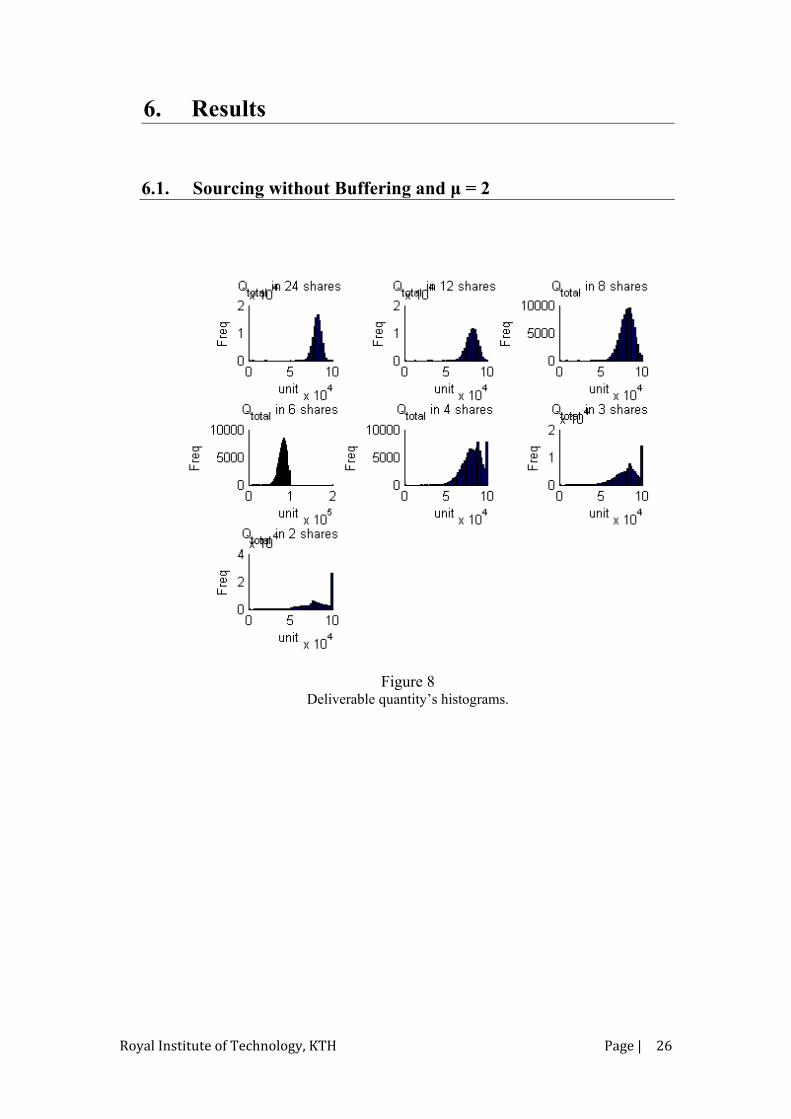
6.1. Sourcing without Buffering and μ = 2

Figure 8

Deliverable quantity’s histograms.


27

Figure 9

Estimated contract cost’s histograms.


28

Figure 10

Deliverable quantity’s CDFs for sourcing without buffering and μ = 2.

24 delivery

12 delivery

8 delivery

6 delivery

4 delivery

3 delivery

2 delivery

Min 0 0 0 0 0 0 0 Max 99573,92 100000 100000 100000 100000 100000 100000 Mean 81790,46 81724,96 81718,59 81784,42 81754,01 81805,66 81770,33 Median 81980,77 82080,85 82290,38 82477,52 82720,74 83742,42 83111,7 Std 4714,858 6681,769 8167,381 9393,801 11497,54 13258,99 16328,82

1% 70189,87 64972,42 60902,28 57321,67 51304,56 46104,56 36570,69 2% 71667,13 67040,81 63438,34 60481,47 55266,29 50806,49 42186,69 5% 73739,28 70173,09 67341,4 65192,1 61092,3 57708,65 51819,98

10% 75632,47 72882,08 70853,29 69260,46 66278,2 63617,41 58772,32 25% 78697,03 77369,52 76430,27 75747,87 74421,05 73177,01 71969,72 50% 81980,77 82080,85 82290,38 82477,52 82720,74 83742,42 83111,7 75% 85083,02 86449,04 87602,09 88607,38 90126,81 91708,22 99012,52 90% 87717,11 90085,48 91874,69 93349,59 96415,86 100000 100000

100% 99573,92 100000 100000 100000 100000 100000 100000

Table 5 Deliverable quantity’s statistics for sourcing without buffering and μ = 2.


29

Figure 11

Overall contract cost CDFs for sourcing without buffering and μ = 2.

24 delivery

12 delivery

8 delivery

6 delivery

4 delivery

3 delivery

2 delivery

Min 0 0 0 0 0 0 0 Max 997105,2 1012537 1021556 1025731 1037935 1045749 1049558 Mean 820964,4 820301,9 820261 820911,3 820591,2 821131,9 820806,5 Median 822873,1 823828,5 825819,2 827671,8 830131,3 840128,4 833889,9 Std 47676,13 67576,89 82595,57 94995,59 116262,1 134103,7 165156,1

1% 703799,8 651097,9 609876,3 574167,4 513864,9 461497,3 365706,9 2% 718617,8 672002,4 635869,9 606002,8 553334,8 508291,5 421866,9 5% 739573,7 703716 674948,1 653282,3 612101,5 578133,6 518614,5

10% 758751,6 730835,9 710468,7 694164,3 664129,4 637271,9 588681 25% 789616,8 776223,8 766756,9 759623,9 746235,5 733731,7 721149 50% 822873,1 823828,5 825819,2 827671,8 830131,3 840128,4 833889,9 75% 854262,1 868031,4 879685 889831,8 905323,8 920837,5 993635,8 90% 880864,9 904867,3 923280,8 938259,4 968885,2 1000000 1002547

100% 997105,2 1012537 1021556 1025731 1037935 1045749 1049558

Table 6 Overall contract cost’s statistics for sourcing without buffering and μ = 2.


30


Figure 12



31

Figure 13



32

Figure 14


24 delivery

12 delivery

8 delivery

6 delivery

4 delivery

3 delivery

2 delivery

Min 25656,01 8333,333 0 0 0 0 0 Max 100000 100000 100000 100000 100000 100000 100000 Mean 92862,96 92864,87 92877,18 92868,38 92851,64 92907,79 92925,17 Median 93123,24 93376,3 93835,56 93663,74 94379,55 96851,88 100000 Std 3157,678 4458,369 5494,129 6315,343 7704,855 8819,946 10817,71

1% 84629,99 80683 77393,49 74318,94 69097,74 65479,22 56781,66 2% 85694,69 82297,23 79609,2 77256,74 72759,25 69636,94 61771,48 5% 87278,29 84736,56 82769,72 80923,98 77946,32 75147,53 71877,56

10% 88702,69 86876,36 85443,29 84276,49 81948,66 81018,69 77115,79 25% 90880,4 90119,44 89566,97 89098,34 88506,91 87200,54 86495,36 50% 93123,24 93376,3 93835,56 93663,74 94379,55 96851,88 100000 75% 95120,35 96171,37 96990,64 98413,19 100000 100000 100000 90% 96709,53 98231,82 100000 100000 100000 100000 100000

100% 100000 100000 100000 100000 100000 100000 100000



33

Figure 15

Overall contract cost’s CDFs for sourcing without buffering and μ = 5.

24 delivery

12 delivery

8 delivery

6 delivery

4 delivery

3 delivery

2 delivery


1% 847935,9 808118,9 774760,9 744590,4 691679 655798,8 568111,2 2% 858593,6 824464,9 797008,5 773675,2 728327,7 697142,1 618156,9 5% 874661,1 848984,5 829155,2 810599,7 780645,7 752474 719317,5

10% 888907,5 870512,1 855991,8 844311,8 821048 811312,4 772618,8 25% 910948,5 903106,7 897599,5 892841,1 886999,6 873814,2 866549 50% 933438,9 936029,4 940270,8 939093,6 946043,7 970754,8 1000000 75% 953603,3 964107,3 972479 986696,8 1000000 1000000 1000000 90% 969688,2 984947,8 1000000 1001116 1003921 1005397 1006069

100% 1007680 1018472 1021473 1030863 1037604 1044170 1048747



34


Figure 16



35

Figure 17



36

Figure 18


24 delivery

12 delivery

8 delivery

6 delivery

4 delivery

3 delivery

2 delivery

Min 41163,81 0 0 33333,33 0 0 0 Max 100000 100000 100000 100000 100000 100000 100000 Mean 94974,67 94952,87 94977,82 95005,08 94983,24 94951,32 94973,32 Median 95233,75 95596,03 95555,68 96003,58 98499,74 100000 100000 Std 2672,796 3779,669 4587,397 5293,428 6500,641 7511,146 9191,205

1% 87672,81 84248,83 81310,64 78796,06 74506,76 70148,45 61492,66 2% 88708,21 85747,74 83459,69 81234,94 77591,65 73586,47 68189,49 5% 90209,2 87949,95 86282,82 84816,44 81809,27 79978,04 76127,9

10% 91434,09 89822,72 88714,65 87508,38 86444,07 84406,06 79974,8 25% 93338,19 92707,06 92355,21 92157,13 90813,97 90403,58 92707,26 50% 95233,75 95596,03 95555,68 96003,58 98499,74 100000 100000 75% 96898,82 97741,58 99163,6 100000 100000 100000 100000 90% 98195,4 99892,44 100000 100000 100000 100000 100000

100% 100000 100000 100000 100000 100000 100000 100000



37

Figure 19

Overall contract cost’s CDFs for sourcing without buffering and μ = 7.

24 delivery

12 delivery

8 delivery

6 delivery

4 delivery

3 delivery

2 delivery

Min 411638,1 0 0 333333,3 0 0 0 Max 1010290 1015897 1020932 1028685 1033971 1045247 1047290 Mean 951532,9 951319,3 951572,5 951837,4 951630 951282 951533,6 Median 954078,3 957728,1 957516,2 961861 986618,5 1000000 1000000 Std 26908,98 38068,04 46199,26 53308,74 65461,43 75637,01 92562,98

1% 878001,9 843621,2 814700 788809,5 745683,1 702539,6 616497,9 2% 888558,2 858780,5 835855,1 813603,1 777239,3 737008,1 682704,7 5% 903662,8 880814,6 864271 849248,1 819012,1 800643,2 762138

10% 915925,7 899722,2 888487,6 876357,9 865599,6 845287,6 800708,4 25% 935026,6 928592,1 925042,8 923109,2 909703,2 905241,6 927900,4 50% 954078,3 957728,1 957516,2 961861 986618,5 1000000 1000000 75% 970893,7 979396,5 993539,1 1000000 1000000 1000000 1000000 90% 983973,7 1000000 1001232 1002658 1004245 1004509 1003335

100% 1010290 1015897 1020932 1028685 1033971 1045247 1047290



38

6.4. Sourcing with 1% Buffering and μ = 5

Figure 20



39

Figure 21



40

Figure 22 Deliverable quantity’s CDFs for sourcing with a buffer = 1% and μ = 5.

24 delivery

12 delivery

8 delivery

6 delivery

4 delivery

3 delivery

2 delivery


1% 88515,64 82452,91 78543,48 75180,57 69782,38 65755,88 57492,09 2% 89600,88 84151,38 80671,03 77888,81 73284,8 69874,62 62688,41 5% 91068,92 86468,18 83688,01 81459,21 78307,18 75079,93 72462,3

10% 92268,2 88400,89 86230,82 84651,82 82019,09 80678,08 77443,45 25% 94149,86 91388,25 90109,56 89195,53 88670,75 87044,59 85516,24 50% 95953,89 94257,21 93838,77 93626,03 93491,81 94799,66 100000 75% 97445,42 96696,97 96728,97 97387,01 100000 100000 100000 90% 98502,93 98342,65 99302,65 100000 100000 100000 100000

100% 100000 100000 100000 100000 100000 100000 100000

Table 11 Deliverable quantity’s statistics for sourcing with a buffer = 1% and μ = 5.


41

Figure 23

Overall contract cost’s CDFs for sourcing with a buffer = 1% and μ = 5.

24 delivery

12 delivery

8 delivery

6 delivery

4 delivery

3 delivery

2 delivery

Min 285641,1 84175,28 0 0 0 0 0 Max 1091066 1060485 1045000 1036659 1033742 1030456 1039509 Mean 977306,9 960322,8 953692 949986,9 945540,9 943126,5 939285,7 Median 980213,1 966867,1 961287,7 959848 969903,5 998355,7 1000000 Std 24469,12 37084,41 47057,38 55587,8 69593,96 82014,03 102102,7

1% 908870,6 850845,6 812361 777128,1 719018,6 675911,8 582182,2 2% 918752,5 868213,3 833557,9 803601,8 758874,4 715213,3 640739,6 5% 933423,2 891153,2 864184 843782,2 806285,8 776610,4 751328,8

10% 945406 910422 890400 873439,1 850479,8 839863,5 785884,3 25% 963297,6 939583,4 927730,9 922619,7 904672,1 892694,2 888348 50% 980213,1 966867,1 961287,7 959848 969903,5 998355,7 1000000 75% 993879,7 987567,8 993235,7 1000000 1000000 1000000 1000000 90% 1005261 1000601 1001562 1002430 1003609 1004160 1003626

100% 1091066 1060485 1045000 1036659 1033742 1030456 1039509

Table 12 Overall contract cost’s statistics for sourcing with a buffer = 1% and μ = 5.


42


Figure 24 Deliverable quantity’s histograms.


43

Figure 25



44

Figure 26

Deliverable quantity’s CDFs for sourcing with a buffer = 1% and μ = 5.

24 delivery

12 delivery

8 delivery

6 delivery

4 delivery

3 delivery

2 delivery

Min 0 24900,95 0 0 0 0 0 Max 100000 100000 100000 100000 100000 100000 100000 Mean 97876,68 95491,34 94306,11 93654,92 93095,93 92765,7 92736,03 Median 98303,28 96193,17 95266,24 94659,61 94396,66 95429,46 100000 Std 2074,293 3571,535 4714,132 5685,409 7154,119 8502,699 10509,42

1% 91737,4 84592,74 79960,29 76235,01 70908,96 65988,19 57510,55 2% 92729,11 86298,68 82100,39 78922,46 74394,17 70241,08 62606,62 5% 94095,37 88660 85312,09 82804,96 79240,36 75627,07 72873,76

10% 95220,84 90642,16 87823,11 85973,35 83009,61 81230,02 78022,9 25% 96843,51 93544,62 91699,83 90500,39 89555,48 87651,37 86239,05 50% 98303,28 96193,17 95266,24 94659,61 94396,66 95429,46 100000 75% 99438,3 98191,4 97837,5 98237,15 100000 100000 100000 90% 100000 99505,76 100000 100000 100000 100000 100000

100% 100000 100000 100000 100000 100000 100000 100000



45

Figure 27


24 delivery

12 delivery

8 delivery

6 delivery

4 delivery

3 delivery

2 delivery

Min 0 250000 0 0 0 0 0 Max 1150000 1120117 1090000 1090000 1060000 1046373 1038804 Mean 996042,2 974996,1 963867,9 957462,5 950780,1 946386,8 941844,4 Median 998421,1 981372,7 972190,4 969240,8 978103,6 1000000 1000000 Std 23971,66 35329,51 45175,78 54055,3 67656,73 80693,07 101191,2

1% 935409,5 866929,7 821838,5 784856,1 729027 678077,3 580077,6 2% 945197 884887,6 844928 812910,1 768081,8 718756,4 638976 5% 958294,9 909224,5 876766,7 852660,8 814258 780998,6 752717

10% 968749,7 928561,6 903129,9 883984,3 857844,8 842405,2 791150,4 25% 983625,9 956803,8 940728,5 931162,1 912847,1 898965,5 895483,6 50% 998421,1 981372,7 972190,4 969240,8 978103,6 1000000 1000000 75% 1004441 1000000 1000000 1000000 1000000 1000000 1000000 90% 1028748 1011374 1002741 1002773 1003441 1003915 1003656

100% 1150000 1120117 1090000 1090000 1060000 1046373 1038804



46




47

Figure 29 Estimated contract cost’s histograms.


48

Figure 30

Deliverable quantity’s CDFs for sourcing with a buffer = 5% and μ = 5.

24 delivery

12 delivery

8 delivery

6 delivery

4 delivery

3 delivery

2 delivery

Min 12500 16666,67 0 0 25000 0 0 Max 100000 100000 100000 100000 100000 100000 100000 Mean 99411,34 98124,92 96931,15 95894,28 94587,54 93881,98 93219,7 Median 100000 99378,25 98693,93 97588,23 96738,45 97559,54 100000 Std 1232,046 2697,55 3959,525 5012,105 6684,595 8069,12 10287,73

1% 95091,13 88790,01 83360,14 78994,04 72038,87 67046,69 57809,7 2% 96006,5 90397,37 85720,85 81857,58 75689,27 71508,9 63174,73 5% 97063,47 92706,45 88922,17 85739,27 81069,14 77316,6 72999,33

10% 97990,22 94482,42 91495,29 89062,27 85226,18 82911,8 78831,26 25% 99181,8 96996,11 95035,59 93432,85 91556,45 89749,01 87430,93 50% 100000 99378,25 98693,93 97588,23 96738,45 97559,54 100000 75% 100000 100000 100000 100000 100000 100000 100000 90% 100000 100000 100000 100000 100000 100000 100000

100% 100000 100000 100000 100000 100000 100000 100000



49

Figure 31


24 delivery

12 delivery

8 delivery

6 delivery

4 delivery

3 delivery

2 delivery

Min 125000 166666,7 0 0 250000 0 0 Max 1092053 1226820 1225000 1158003 1150000 1090390 1075000 Mean 995907,6 994149,7 985641,1 975843,4 962722,8 954850,9 945272,6 Median 1000000 1000000 1000000 995311,4 1000000 1000000 1000000 Std 13095,57 33095,53 43842,24 52146,28 66526,37 79380,57 101284,7

1% 954488,1 901116 851128,5 806052,3 732260,6 680818,5 579007,7 2% 962843,1 918359,5 874627,7 836093,8 773651,2 726281,6 637916 5% 973323,9 939346,5 905115,3 875387,8 828129,1 792223,8 750793,8

10% 981383,9 958751,9 933311,2 910027 876350,7 847172,5 800477,2 25% 994757,8 981545,1 966452,9 954268,1 933928,7 916887,1 905012,3 50% 1000000 1000000 1000000 995311,4 1000000 1000000 1000000 75% 1000000 1000000 1000000 1000000 1000000 1000000 1000000 90% 1000055 1024821 1020587 1003824 1003112 1003175 1002875

100% 1092053 1226820 1225000 1158003 1150000 1090390 1075000



50




51

Figure 33



52

Figure 34 Deliverable quantity’s CDFs for sourcing with a buffer = 10% and μ = 5.

24 delivery

12 delivery

8 delivery

6 delivery

4 delivery

3 delivery

2 delivery

Min 4166,667 0 0 0 0 0 0 Max 100000 100000 100000 100000 100000 100000 100000 Mean 99553,09 99007,15 98290,16 97535,17 96332,68 95279,75 94062,65 Median 100000 100000 100000 100000 100000 100000 100000 Std 1150,343 2135,675 3251,288 4313,251 6085,503 7599,711 9949,759

1% 95702,75 91096,19 85930,69 81463,94 74322,44 68058,83 57840,11 2% 96451,82 92608,84 88367,66 84566,41 78043,17 72224,4 63402,26 5% 97574,81 94740,92 91485,38 88450,68 83442,24 79290,32 73956,76

10% 98224,33 96271,54 94075,88 91891,24 88033,5 84528,57 79258,74 25% 99766,32 98926,2 97635,4 96151,78 94164,11 93210,8 90154,6 50% 100000 100000 100000 100000 100000 100000 100000 75% 100000 100000 100000 100000 100000 100000 100000 90% 100000 100000 100000 100000 100000 100000 100000

100% 100000 100000 100000 100000 100000 100000 100000



53

Figure 35 Overall contract cost’s CDFs for sourcing with a buffer = 10% and μ = 5.

24 delivery

12 delivery

8 delivery

6 delivery

4 delivery

3 delivery

2 delivery

Min 41666,67 0 0 0 0 0 0 Max 1060677 1151477 1292468 1303010 1300000 1165742 1150000 Mean 995692,9 991773,8 989276 986426,3 976502,6 965631,6 951720,8 Median 1000000 1000000 1000000 1000000 1000000 1000000 1000000 Std 11514,8 22415,06 38105,68 51491,53 67316,48 80491,11 101830

1% 957574,3 913196,7 866002,4 823510,5 752975,3 684737 578558,9 2% 964819,8 928199,2 890184,9 854527,6 789311 728633,8 635972 5% 976071,6 949902,3 922217,7 895123 847919,6 804113,6 751011,9

10% 982437,9 964290,2 944937,3 926120 889440,7 855031,7 801705,4 25% 998125,7 992981,9 985003,4 975812,7 963395 946735,2 926093,8 50% 1000000 1000000 1000000 1000000 1000000 1000000 1000000 75% 1000000 1000000 1000000 1000000 1000000 1000000 1000000 90% 1000000 1000000 1000411 1001432 1001745 1001955 1001839

100% 1060677 1151477 1292468 1303010 1300000 1165742 1150000



54

7. Discussion

The results of the Monte Carlo simulation are reflected in histograms and

cumulative distribution function (.i.e. CDF). We can clearly see that as M (i.e. M is the number of sub deliveries of the whole ordered quantity totalQ ) changes, the shape of the histograms does as well. The supplier simulated capacity (.i.e. supplier simulated capacityµ is the expectation of the random variables aq and bq )

introduces significant changes in the results as well. So does the buffer size for the case of souring with buffering.

For the case of sourcing without buffering, it is easily seen that for a given supplier’s expected capacity xµ , the samples are distributed more on the right toward totalQ as M tends toward smaller values (i.e. as goods are supplied less

often but in higher quantities). We see in Table 4, that the delivered quantity median values for the case where µ = 2, increase from 81980.77 unit for M =24 to

83111.7 units for M = 2. The increase in noticeable for all percentile values superior to 50%, on the other hand the values of lower percentiles are better for higher values of M which suggest that an improvement in the likelihood of not having default happens as goods are delivered with a value of M between 2 and 24..

An improvement of the same nature is noticeable as the simulated expected

supplier capacity increases from 2 till 7. This improvement was expected, but could not be quantified without simulation. The median values of the delivered total quantities supplied in 24 sub-deliveries (i.e. see Table 4, Table 6 and Table 8) are 81980.77, 93123.25 and 95233.75 for simulated suppliers’ capacities being 2, 5, and 7 times higher than the ordered quantities.

Figure 9, illustrates the simulated contract overall cost for sourcing without buffering and supplier’s expected capacityµ = 2.

As for the corresponding quantities of Figure 8, the prices increase as the delivered quantities do.

Figure 10 shows a continuous improvement in the sharpness of the CDFs as the numbers of splits is reduced, at the same time, the median (i.e. the 50% percentile) is a little larger than 80 000 unit and is very close to some points in which curves cross.

Figure 11 shows possible excess for the cost of contracts. The excess starts at 90% percentile, for schemes with two splits. The Excess decreases as the number of splits increases.


55

Table 6, presents the numerical values of the overall cost CDF, we can see that the maximal cost value can increase by 4.9% when the quantity is split in two shares and 1.2% while split in 12 shares. When totalQ is split in 24 shares the overall cost CDF, shows that the maximal value is 997105, which is due to the not satisfactory amount of delivered goods.

As soon as buffering is used, we can notice a clear improvement in the histograms patterns, which values have the tendency to be distributed closer to the upper limit totalQ . As the Buffer size is increased from 1%, 2%, 5% and 10% of totalQ , the histogram samples get closer to totalQ .

For the case of buffering 1% of totalQ , as shown in Figure 26, the probability of having goods quantities between values close to

totalQ becomes very large. This is seen in the sharp vertical lines of the CDFs for M=2 and M=3. The CDFs for larger buffer sizes looks likes inverted “L”, which demonstrated the tremendous improvements.

For every value of M, the deliverable quantity statistics improve as the buffer

size increases too, but at the expense of an excess in the possible cost. This is due to the increased likelihood of buffering quantities which will probably not be of any use. , Comparing the performance of sourcing with and without buffering for the same suppliers capacity µ = 5, we can see that 2% buffering does increase the

performance when M =2, but with a small margin. This suggests further comparison of buffering vs. ordering larger quantities. The performance of sourcing with 1% buffering at M=2 is close to sourcing with 2% buffering at M= 6 and sourcing with 5% buffering and M= 12. This suggests that instead of ordering large quantities less often, we can order less goods more often and but buffer more. These compromises are possible to quantify only if costs of buffering and stocking goods are available.


56

8. Conclusions and Recommendations

Two sourcing schemes have been simulated to determine their performances

with respect to different variables. The problem encountered was to determine the optimal variation of parameters to obtain the best statistics at the lowest cost. Buffering proves to be a very powerful mitigation method, but it is has a cost reflected in cost excess as seen in the cost CDFs. While splitting a total ordered quantity in larger shares and ordering larger quantities less often, costs are introduced, such as stocking and in some cases preserving goods. These costs have not been included in our simulation, nevertheless, it has been shown that the problem is multidimensional and can be solved using modeling and simulation. When stocking and preserving goods is not expensive, it is recommended to order more quantities but less often with less buffering (.i.e. reduced over provisioning). On the other hand when goods are expensive and can be over provisioned as compared to what it would cost to stock them, buffering is a better way to go. The model and the simulator can be use to calculate the statistics of the different schemes and obtain comparative results for finding the optimal solution.

There is a need to develop the mathematical bases of the proposed algorithm, by exploring the use of other distributions for the sample generation. We have modeled the supplied quantity using a geometric distribution, which is a reasonable choice, but for other conditions, this choice might not be appropriate. In an environment where supply is subject to a large number of stochastic influences, the normal distribution could be a better choice. It is recommended to do the same work with different distributions and compare the results.

This work was inspired of previously done work [2], but was improved to include more variations and introduce the effect of buffering. It is recommended, to use the model and simulator of this thesis work to explore realistic cases where cost of stocking and different “overheads” are included, this will certainly result in a tool capable of optimizing sourcing by saving tremendous budgeting and insuring continuous and prosper supply.


57

Bibliography

[1] A guide to the project management body of knowledge. PMI Standards Committee.

[2] Choosing between single and multiple sourcing based on supplier default risk: A real options approach: Nicola Costantino, Roberta Pellegrino.

[3] Monte Carlo methods. John Michael Hammersley,David Christopher Handscomb

[4] A first Course in Monte Carlo. George S. Fishman.

[5] Multiple sourcing vs single sourcing, Madhusudan Partani, 2010.

[6] Single and multi-sourcing models. C Ford, A Maughan, S Stevensson Morrisson & Foerster LLP.

[7] http://en.wikipedia.org/wiki/Redundancy_(engineering)

[8] ]. Standards Australia and Standards New Zealand (2004). Risk Management. AS/NZS 4360:2004.

[9] Introduction to Probability. Dimitri Bertsekas, John N tsitsiklis. MIT Press

http://en.wikipedia.org/wiki/Redundancy_(engineering)


58

Appendices

Appendix A: Probability Distributions

As we have seen in the previous IMC algorithm, sampling comes from random number generators obeying well chosen probability distributions. In the case of mean calculations, a uniform distribution is used.

Probability distributions are different and each one corresponds to an event

scenario. Some distributions are introduced in Appendix A. A distribution function has certain properties as summarized below:

It is always positive Integration over the overall region is equal to unity when the distribution is

deduced analytically. When it is a result of sampling it must be normalized. It can be deduced of a certain probability event or not. When it is discrete it is called probability mass function When it is continuous it is called probability density function.

It is essential to choose the right probability distribution function to model a

random variable, and to justify the choice. When there is a lack of knowledge on the nature of the random variable in question, or when it is not possible to develop an analytical model for it, approximate distributions are used. When the nature of randomness is not possible to distinguish, the Normal (aka Gaussian) distribution is usually used. The central limit theorem states that the result of a very large summation of identically distributed random variable can be modeled using a Gaussian distribution.

1. Continuous Uniform: The uniform distribution is used when we know the intervals from which samples are obtained. These samples have the same likelihood of occurrence

+=

−−=otherwise

baakifabkPX

,0

,....1.,1

1)( (9)

a. Mean: 2

ba +=µ (10)

b. variance: 12

)( 22 ab −=σ (11)


59

2. Bernoulli with parameter p: The Bernoulli describes events with success or failure in single trials.

=−=

=0,11,

)(kifpkifp

kPX (12)

a. Mean: p=µ (13) b. Variance: )1(2 pp −=σ (14)

3. Binomial with parameter p and n: Describes the number of trials until the first success in a sequence of independent Bernoulli trials

( ) knkX pp

kn

kP −−

= )1( k= 0,1,………….,n (15)

a. Mean: np=µ (16)

b. Variance: )1(2 pnp −=σ (17)

4. Geometric with parameter p Describes the number of trials until the first success in a sequence of independent Bernoulli trials

ppkP kX

1)( −= k=1…….., (18)

a. Mean: p1

=µ (19)

b. Variance: 22 1

pp−

=σ (20)

5. Poisson with parameter λ Approximate the binomial when n is very large and p is small, and λ=np

!)( kX

k

ekPλ

λ−= k =1……, (21)


60

a. Mean: λµ = (22) b. Variance: λµ = (23)

6. Exponential with parameter λ Describes the time until the first success in a continuous time interval

≥

=−

otherwisexife

fx

X ,00,λλ

(24)

a. Mean: λ

µ 1= (25)

b. Mean: 22 1

λσ = (26)

7. Gaussian random with mean µ and standard deviation σ

Is used to models random contributions due to numerous unknown but identically distributed random variables

2

2

2)(

21 σ

µ

σπ

−−=

x

X ef (27)

a. Mean: µ (28)

b. Variance: 2σ (29)


61

Appendix B: Monte Carlo Simulations

B1: Monte Carlo Simulations

In a stochastic model, random variables can be the resultant of a large number of other variables. To evaluate a random variable which is the combination of other variables, analytical methods can be used but if the model is complex this can become very tedious if not impossible. The probability distribution of the sum of two random variables X and Y is analytically an easy task to resolve.

If Z, X, and Y are three random variables with X and Y having probability distributions )(xf and )(yg respectively, if Z = X + Y, then the distribution h of Z is the convolution of f and g [9]:

gfh ∗= (1)

When the resultant random variable is a successive summation of RVs, the convolution theorem can be used to compute the distribution of the resultant variable. On the other hand when the resultant random variable is not a summation but the nonlinear combination of many other random variables, then Monte Carlo simulation becomes the ultimate choice for such mathematical problem. It is a powerful method that provides very straightforward results with acceptable confidence. The next subsections are an introduction to Monte Carlo simulation and the mathematics behind it.

B2 : Theory and Application of Monte Carlo Simulations

Monte Carlo Simulation is a branch of mathematics; often referred to as

experimental mathematics. While mathematics used deductions from postulates, Monte Carlo simulation is based on generating pseudo-random numbers to find solutions. There exist two types of Monte Carlo simulations, one where the problem is deterministic and one where it is random.

For probabilistic matters, Monte Carlo Simulation is used to generate random numbers using a collection of techniques to directly emulate physical random behaviors. The following examples present cases where Monte Carlo simulations can be used [3].


62

Insect population growth according to certain vital statistics: The advantage of using Monte Carlo is a significant gain of time, because the growth time is omitted

Design of telephone exchanges and simulations of call arrival patterns. The simulation in this case emulates users and saves using testers.

Radio performance testing where hardware is subject to recursive strains and performance parameters are logged and displayed in histograms.

Simulation of nuclear reactors performance using random numbers to simulate neutron dynamics.

Monte Carlo can be used using different approach [3]. It is very hard to define

a single one. However most of the methods make use of the following methodology.

1. Possible input domain definition 2. Random input generation from the domain using specified probability

distributions: The simulation during each iteration generates one random value out of a random number generator ruled by a modeling distribution function

3. Deterministic Computation using the input: The random input is fed to an arithmetic function or combined in a simulation algorithm to produce the resultant random variable.

4. Result aggregation: The result is aggregated in the form of a histogram and cumulative distribution function out of which probabilities can be computed.

B3: Estimating a Mean using the Independent Monte Carlo

Monte Carlo Simulation can be used to estimate a mean of a population. The following is an example of an algorithm which provide a solution to an

integral, this algorithm can be used to solve other problems which can be stated mathematically [2].

Let’s suppose we have an integral of the following form representing a mean calculation.

∫=x

dxxgy )( (2)

We assume that the integral is bounded that is ∞<∫ dxxg

x

)(2

Let ω denote a probability density function such as the mean µ is obtained by


63

µωω =

)()(

XXgE (3)

To estimate the mean the following algorithm can be used it is called the

independent Monte Carlo, IMC [2].

Given a number n := number of replications3 Method: i=1 While :ni ≤

Randomly generate:

( ))()(1

)( ,......,: im

ii XXX = Independently from ω

Evaluate: ( )( ))(

)(

i

i

XXg

ω

i=i+1 Compute:

( )( )∑

=

=n

ii

i

n XXg

n 1)(

)(1:ω

µ (4)

As n tend to ∞ µµ →n µ is the mean and not an estimate of it.

3 Replications here mean iterations of sample generations.

Risk Analysis and Optimization of Dual- Sourcing with ...608004/FULLTEXT01.pdf · Risk Analysis and...

Documents

Transcript of Risk Analysis and Optimization of Dual- Sourcing with ...608004/FULLTEXT01.pdf · Risk Analysis and...