ABSTRACT

HOANG, PHUONG. Supervised Learning in Baseball Pitch Prediction and Hepatitis CDiagnosis. (Under the direction of Hien T. Tran.)

Machine learning is so ubiquitous nowadays that one probably uses it multiple times

during the day without realizing it. For example, it is used in web search engines to improve

efficiency, by email providers to identify junk emails, and in voice recognition, among others.

Machine learning is a powerful tool that can be used to analyze large amount of data to

make actionable predictions. Since machine learning uses algorithms that iterate on data,

the quality and quantity of training data are important factors for accurate predictions. In

particular, the data available for baseball pitch prediction is huge, millions of observations

(pitches) each containing more than fifty features. However, the prediction task restricts

researchers to working only with the less than ideal features that were measured before the

target pitch is thrown. In addition, the presence of noise in pitch type labels makes it even

harder to train classifiers. Meanwhile, the dataset for Hepatitis C is fairly small with less

than two hundreds observations and 20 features. This disadvantage prevents researchers

from removing observations with low quality when building reliable diagnosis models.

Hence, prediction problems in the presence of missing features are pervasive in machine

learning. This thesis focuses on a number of classification methods and other machine

learning tools, and tailor them to address the above issues specifically.

First, in the pitch prediction problem, unlike the current method which suggests a

static feature selection algorithm for each pitcher, we propose a novel dynamic feature

selection procedure that is shown to be more adaptive for each pitcher in each count. The

tradeoff is that the size of training data is reduced dramatically with pitcher-count data

segmentation. Thus, we propose a simple heuristic approach for constructing and selecting

features to include during training that are shown to surpass this tradeoff, which in turn

yields considerable improvement in prediction accuracy.

In the second part of the thesis, we propose a new learning algorithm for Hepatitis C

diagnosis that addresses the important issue of class imbalance. Most existing learning algo-

rithms simply ignore the presence of class imbalance due to the lucrative high accuracy that

can be easily attained. The current method suggests combining over-sampling (minority

class) and weighted cost in Support Vector Machine. Through our research study, however,

we were able to show that doing both is unnecessary. We choose only to employ the later

but add the parameter optimization procedure to improve classification performance. Our

experimental results show that our proposed method is more accurate and reliable than

the existing learning methods.

Supervised Learning in Baseball Pitch Prediction and Hepatitis C Diagnosis

byPhuong Hoang

A dissertation submitted to the Graduate Faculty ofNorth Carolina State University

in partial fulfillment of therequirements for the Degree of

Doctor of Philosophy

Applied Mathematics

Raleigh, North Carolina

2015

APPROVED BY:

Carl Meyer Negash Medhin

Ernie Stitzinger Hien T. TranChair of Advisory Committee

DEDICATION

This thesis is dedicated to my parents, my wife, my son and Odisg.

ii

BIOGRAPHY

Phuong Hoang was born in Saigon, Vietnam on September 3, 1985. He went to the United

States at the age 17 spending a year as an exchange student in Hartford high school, Michi-

gan. In 2005, he started his undergraduate studies at University of Bridgeport, Connecticut

in Business Administration before seeing the light and switching to mathematics in the

second year. He later transferred to North Carolina State University and earned a B.S. in

applied mathematics with financial mathematics concentration in May 2010. During his

undergraduate studies, he interned at Sony Ericsson as a software tester on the GPS team.

After graduation, he continued on at NC State for graduate school in applied mathematics.

During his doctoral studies, he served as a REU graduate assistant for three summers. In his

spare time, he manages of an e-commerce store that sells and trades textbooks and house-

hold electronics. He is also an avid photographer and has volunteered to be a cameraman

on a few research workshops.

iii

ACKNOWLEDGEMENTS

First and foremost, I would like to thank my advisor Dr. Hien Tran for his guidance, encour-

agement, and support during the past 10 years. I deeply appreciate his great patience and

the freedom he gave me to pursue new ideas, many of which were made into this thesis.

His enthusiasm, persistence and expertise on research guided me throughout my doctoral

study, from brainstorming ideas to doing experiments and writing technical papers, among

many other things.

I would also like to thank my thesis committee members, Dr. Carl Meyer, Dr. Negash

Medhin, and Dr. Ernie Stitzinger for their valuable feedbacks on this thesis. Especially, Dr.

Meyer’s fruitful lectures play a big role in keeping my love with applied mathematics.

Special thanks go to my undergraduate advisors Dr. Jeff Scroggs and Dr, Sandra Paur. I

consider successful completion of Dr. Paur’s analysis courses to be my best achievement

in undergraduate study. I also owe to her for guiding me to graduate school and making

sure it happens. I would also like to acknowledge Dr. H. T. Banks who provided me with a

research fellowship during the third year of my Ph.D. program.

Graduate school would not have been the same with my colleagues Mark Hunnell, Rohit

Sivaparasad, Hansi Jiang, Glenn Sidle and George Lankford. Besides our many fun social

activities, they were always a useful sounding board when tackling theoretical questions. I

wish to thank my former REU students, Michael Hamilton, Joseph Murray and Shar Shuai.

Mentoring those who are smarter than I am has helped me in many ways, especially in

finding better solution for a "solved" problem by looking at them from a different angle.

Thanks also go to the research mentors from MIT Lincoln Laboratory Dr. Lori Layne and

Dr. David Padgett for whom I was lucky enough to work with for two summers.

There are many friends who have helped me immeasurably throughout my student life.

A few deserve special recognition. Nhat-Minh Phan who helped me in scrapping data that

I used in this thesis and Nam Tran was always there for me, whether helping me financially

during the rainy day or "shipping" his wife to Raleigh to help my wife and babysit my son

when I were away for conferences. Particular thanks also go to Quoc Nguyen and Thanh

Nguyen for putting up with me throughout the years. Also I would like to thank Dung Tran

and Sombat Southivorarat for being excellent readers of this thesis.

My biggest thanks go to my loving and supportive parents, my wife and my son. This

thesis is dedicated to them. Thank you for sharing this journey with me.

iv

TABLE OF CONTENTS

LIST OF TABLES . . . . . . . . . . . . . . . . . . . . . . . . . . . . . . . . . . . . . . . . . . . . . . . . . . vii

LIST OF FIGURES . . . . . . . . . . . . . . . . . . . . . . . . . . . . . . . . . . . . . . . . . . . . . . . . . viii

Chapter 1 Introduction . . . . . . . . . . . . . . . . . . . . . . . . . . . . . . . . . . . . . . . . . . . 11.1 Statement of the Problems . . . . . . . . . . . . . . . . . . . . . . . . . . . . . . . . . . . . 11.2 Dissertation Outline . . . . . . . . . . . . . . . . . . . . . . . . . . . . . . . . . . . . . . . . . 21.3 Summary of Contributions . . . . . . . . . . . . . . . . . . . . . . . . . . . . . . . . . . . . 3

Chapter 2 Classification . . . . . . . . . . . . . . . . . . . . . . . . . . . . . . . . . . . . . . . . . . 42.1 k -Nearest Neighbors . . . . . . . . . . . . . . . . . . . . . . . . . . . . . . . . . . . . . . . . 72.2 Linear Discriminant Analysis . . . . . . . . . . . . . . . . . . . . . . . . . . . . . . . . . . 102.3 Support Vector Machines . . . . . . . . . . . . . . . . . . . . . . . . . . . . . . . . . . . . . 13

2.3.1 Linear Separable Case . . . . . . . . . . . . . . . . . . . . . . . . . . . . . . . . . . 132.3.2 Nonseparable Case - Soft Margin SVM . . . . . . . . . . . . . . . . . . . . . . 182.3.3 Nonlinearly Separable Case - Kernel trick . . . . . . . . . . . . . . . . . . . . 22

Chapter 3 Overfitting . . . . . . . . . . . . . . . . . . . . . . . . . . . . . . . . . . . . . . . . . . . . 283.1 Regularization . . . . . . . . . . . . . . . . . . . . . . . . . . . . . . . . . . . . . . . . . . . . . 303.2 Validation . . . . . . . . . . . . . . . . . . . . . . . . . . . . . . . . . . . . . . . . . . . . . . . . 33

3.2.1 Hold-Out Validation . . . . . . . . . . . . . . . . . . . . . . . . . . . . . . . . . . . 343.2.2 Cross Validation . . . . . . . . . . . . . . . . . . . . . . . . . . . . . . . . . . . . . . 35

Chapter 4 Baseball Pitch Prediction . . . . . . . . . . . . . . . . . . . . . . . . . . . . . . . . . 374.1 PITCHf/x Data . . . . . . . . . . . . . . . . . . . . . . . . . . . . . . . . . . . . . . . . . . . . . 384.2 Related Work . . . . . . . . . . . . . . . . . . . . . . . . . . . . . . . . . . . . . . . . . . . . . . 384.3 Our Model . . . . . . . . . . . . . . . . . . . . . . . . . . . . . . . . . . . . . . . . . . . . . . . . 41

4.3.1 Dynamic Feature Selection Approach . . . . . . . . . . . . . . . . . . . . . . . 414.3.2 Model Implementation . . . . . . . . . . . . . . . . . . . . . . . . . . . . . . . . . 434.3.3 ROC Curves . . . . . . . . . . . . . . . . . . . . . . . . . . . . . . . . . . . . . . . . . 444.3.4 Hypothesis Testing . . . . . . . . . . . . . . . . . . . . . . . . . . . . . . . . . . . . 464.3.5 Classification . . . . . . . . . . . . . . . . . . . . . . . . . . . . . . . . . . . . . . . . 47

4.4 Results Analysis . . . . . . . . . . . . . . . . . . . . . . . . . . . . . . . . . . . . . . . . . . . . 474.4.1 Overall Results . . . . . . . . . . . . . . . . . . . . . . . . . . . . . . . . . . . . . . . 474.4.2 By Count Analysis . . . . . . . . . . . . . . . . . . . . . . . . . . . . . . . . . . . . . 494.4.3 By Pitcher Analysis . . . . . . . . . . . . . . . . . . . . . . . . . . . . . . . . . . . . 494.4.4 By Noise Level . . . . . . . . . . . . . . . . . . . . . . . . . . . . . . . . . . . . . . . . 52

Chapter 5 Medical Diagnosis . . . . . . . . . . . . . . . . . . . . . . . . . . . . . . . . . . . . . . . 545.1 Previous Work . . . . . . . . . . . . . . . . . . . . . . . . . . . . . . . . . . . . . . . . . . . . . 55

v

5.2 Class Imbalance and Related Work . . . . . . . . . . . . . . . . . . . . . . . . . . . . . . 575.3 Model Implementation . . . . . . . . . . . . . . . . . . . . . . . . . . . . . . . . . . . . . . . 60

5.3.1 Data Preprocessing . . . . . . . . . . . . . . . . . . . . . . . . . . . . . . . . . . . . 605.3.2 Cost Sensitive SVM . . . . . . . . . . . . . . . . . . . . . . . . . . . . . . . . . . . . 635.3.3 Parameters Optimization . . . . . . . . . . . . . . . . . . . . . . . . . . . . . . . . 645.3.4 Evaluation Metrics . . . . . . . . . . . . . . . . . . . . . . . . . . . . . . . . . . . . 66

5.4 Results Analysis . . . . . . . . . . . . . . . . . . . . . . . . . . . . . . . . . . . . . . . . . . . . 66

Chapter 6 Conclusion and Future Work . . . . . . . . . . . . . . . . . . . . . . . . . . . . . . . 726.1 Pitch Prediction . . . . . . . . . . . . . . . . . . . . . . . . . . . . . . . . . . . . . . . . . . . . 726.2 Hepatitis Diagnosis . . . . . . . . . . . . . . . . . . . . . . . . . . . . . . . . . . . . . . . . . 74

BIBLIOGRAPHY . . . . . . . . . . . . . . . . . . . . . . . . . . . . . . . . . . . . . . . . . . . . . . . . . . 76

APPENDICES . . . . . . . . . . . . . . . . . . . . . . . . . . . . . . . . . . . . . . . . . . . . . . . . . . . . 82Appendix A Baseball Pitch Prediction . . . . . . . . . . . . . . . . . . . . . . . . . . . . 83

A.1 Features in Groups . . . . . . . . . . . . . . . . . . . . . . . . . . . . . . . . . . . . . . 83A.2 Baseball Glossary and Info . . . . . . . . . . . . . . . . . . . . . . . . . . . . . . . . 88A.3 Software . . . . . . . . . . . . . . . . . . . . . . . . . . . . . . . . . . . . . . . . . . . . . 89

Appendix B Hepatitis C Diagnosis . . . . . . . . . . . . . . . . . . . . . . . . . . . . . . . 90B.1 Definitions of Attributes . . . . . . . . . . . . . . . . . . . . . . . . . . . . . . . . . . 90

vi

LIST OF TABLES

Table 2.1 Frequently Used Notation, adapted from [1, 12, 37, 57] . . . . . . . . . . . 6Table 2.2 Accuracy and speed comparison of k -NN method using different metrics 8

Table 4.1 List of original attributes selected for pitch prediction . . . . . . . . . . . 39Table 4.2 Data for each pitcher. . . . . . . . . . . . . . . . . . . . . . . . . . . . . . . . . . . . 50Table 4.3 Prediction accuracy comparison (percents). Symbols: k -Nearest Neigh-

bors (k -NN), Support Vector Machine with linear kernel (SVM-L), Sup-port Vector Machine with Gaussian kernel (SVM-G), Naive Guess (NG). 50

Table 4.4 CPU Times (seconds) . . . . . . . . . . . . . . . . . . . . . . . . . . . . . . . . . . . 51Table 4.5 Best Improvement over Naive Guess (percents) . . . . . . . . . . . . . . . . 51Table 4.6 Prediction results by Type Confidence levels (TC). Symbol: k -Nearest

Neighbors (k -NN), Support Vector Machine with linear kernel (SVM-L), and with Gaussian kernel (SVM-G), Linear Discriminant Analysis(LDA). . . . . . . . . . . . . . . . . . . . . . . . . . . . . . . . . . . . . . . . . . . . . . . 52

Table 5.1 Hepatitis C classification accuracies comparison among recent studies. 56Table 5.2 Breast cancer classification accuracies comparison among recent stud-

ies. . . . . . . . . . . . . . . . . . . . . . . . . . . . . . . . . . . . . . . . . . . . . . . . . . 57Table 5.3 Hepatitis C data: description of attributes. See Appendix B.1 for the

definitions of some of the attributes. . . . . . . . . . . . . . . . . . . . . . . . . 62Table 5.4 The table shows the sensitivity and specificity comparison between

algorithms: Support Vector Machines (SVM), Under-sampling (US),Different Error Costs (DEC), SMOTE with Different Costs (SDC). . . . . 69

Table 5.5 The table shows the G-Mean comparison between algorithms: Sup-port Vector Machines (SVM), Under-sampling (US), Different ErrorCosts (DEC), SMOTE with Different Costs (SDC). . . . . . . . . . . . . . . . 69

vii

LIST OF FIGURES

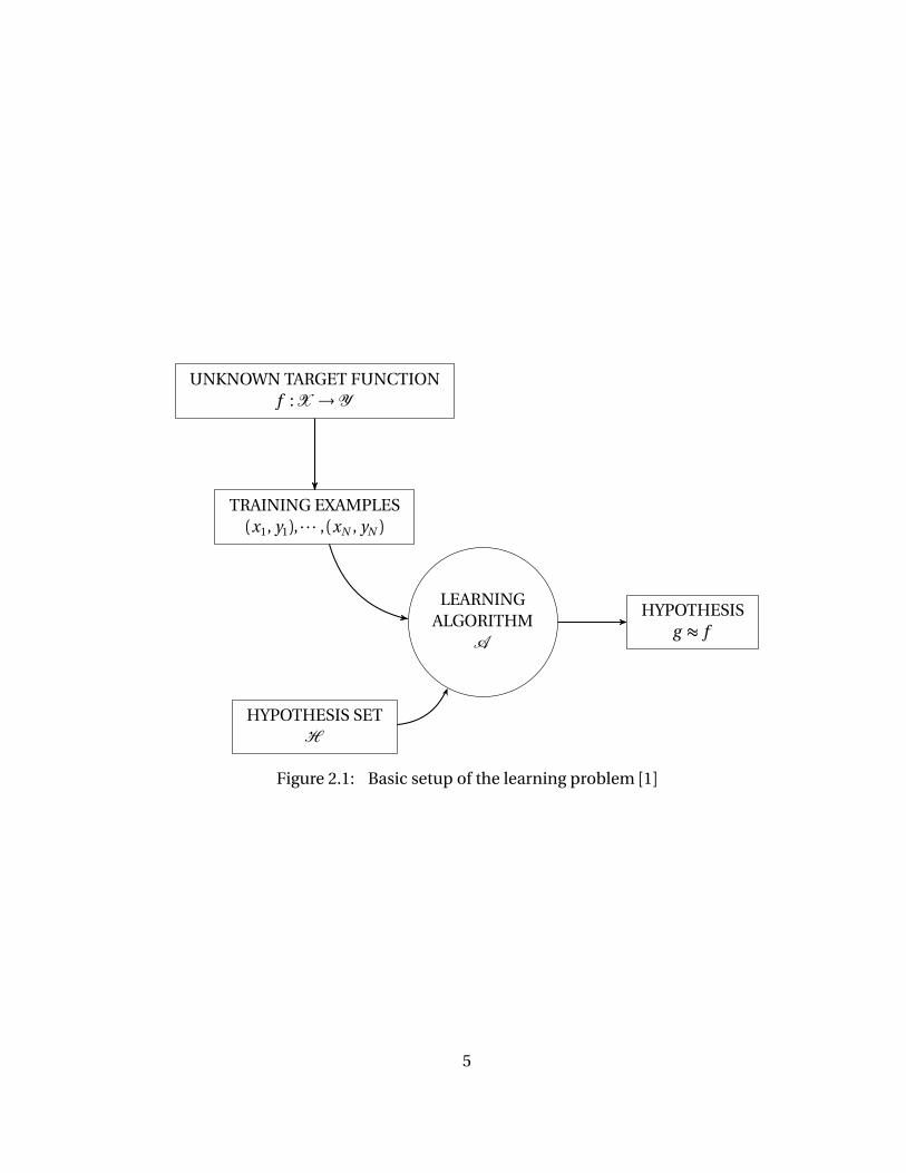
Figure 2.1 Basic setup of the learning problem [1] . . . . . . . . . . . . . . . . . . . . . . 5Figure 2.2 An example of k -NN; using the 7-NN rule, the unknown data point

in red is classified to the black class. Out of the seven nearest neigh-bors, five are of black class and two are of white class (the dashedcircle denotes the region that contains the 7 nearest neighbors of theunknown data point). . . . . . . . . . . . . . . . . . . . . . . . . . . . . . . . . . . 7

Figure 2.3 An example of binary classification problem. Data from class 1 (blue)favor the y -axis while data from class 2 (red) spread out the alongthe North East direction. The unknown data (black) is to be classifiedwith k -NN. . . . . . . . . . . . . . . . . . . . . . . . . . . . . . . . . . . . . . . . . . . 9

Figure 2.4 An example of LDA. Two one-dimensional density functions areshown. The dashed vertical line represents the Bayes decision bound-ary. The solid vertical line represents the LDA decision boundary es-timated from training data. The source code used to make this figureis adapted from [58], used under CC0 1.0, via Wikimedia Commons. 12

Figure 2.5 An example of a linearly separable two-class problem with SVM. Thesource code used to make this figure is adapted from [51]. . . . . . . . . 14

Figure 2.6 An example of a linearly nonseparable two-class problem with SVM.The incorrectly classified data points are enclosed in blue circle. Thesource code used to make this figure is adapted from [51]. . . . . . . . . 19

Figure 2.7 Kernels are used for mapping a non-linearly separable problem intoa higher dimension linearly separable problem. The source codeused to make this figure is adapted from [50]. . . . . . . . . . . . . . . . . . 22

Figure 2.8 An example of kernel trick. . . . . . . . . . . . . . . . . . . . . . . . . . . . . . . . 23

Figure 3.1 Example showing overfittting of a classifier by Chabacano, used underCC BY-SA, via Wikimedia Commons [17]. The green curve separatesthe blue and the red dots perfectly in this (training) data set, hence ithas lower Ein than that of the black curve. However, it also modelsthe noise at the boundary in addition to model the underlying trend.Hence, it will more likely perform poorly on a new data set from thesame population, has higher Eout. The green curve is an example ofan overfitted classifier. . . . . . . . . . . . . . . . . . . . . . . . . . . . . . . . . . 29

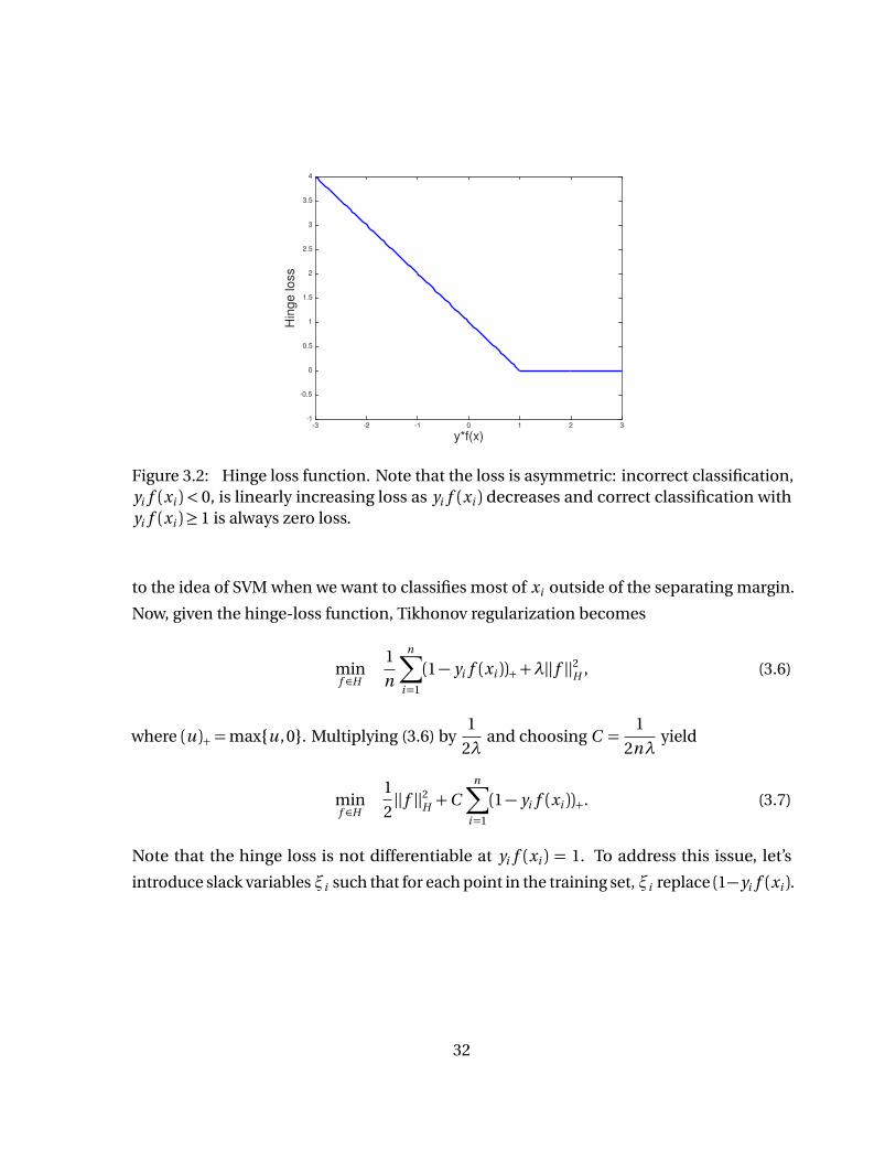
Figure 3.2 Hinge loss function. Note that the loss is asymmetric: incorrect clas-sification, yi f (xi )< 0, is linearly increasing loss as yi f (xi ) decreasesand correct classification with yi f (xi )≥ 1 is always zero loss. . . . . . . 32

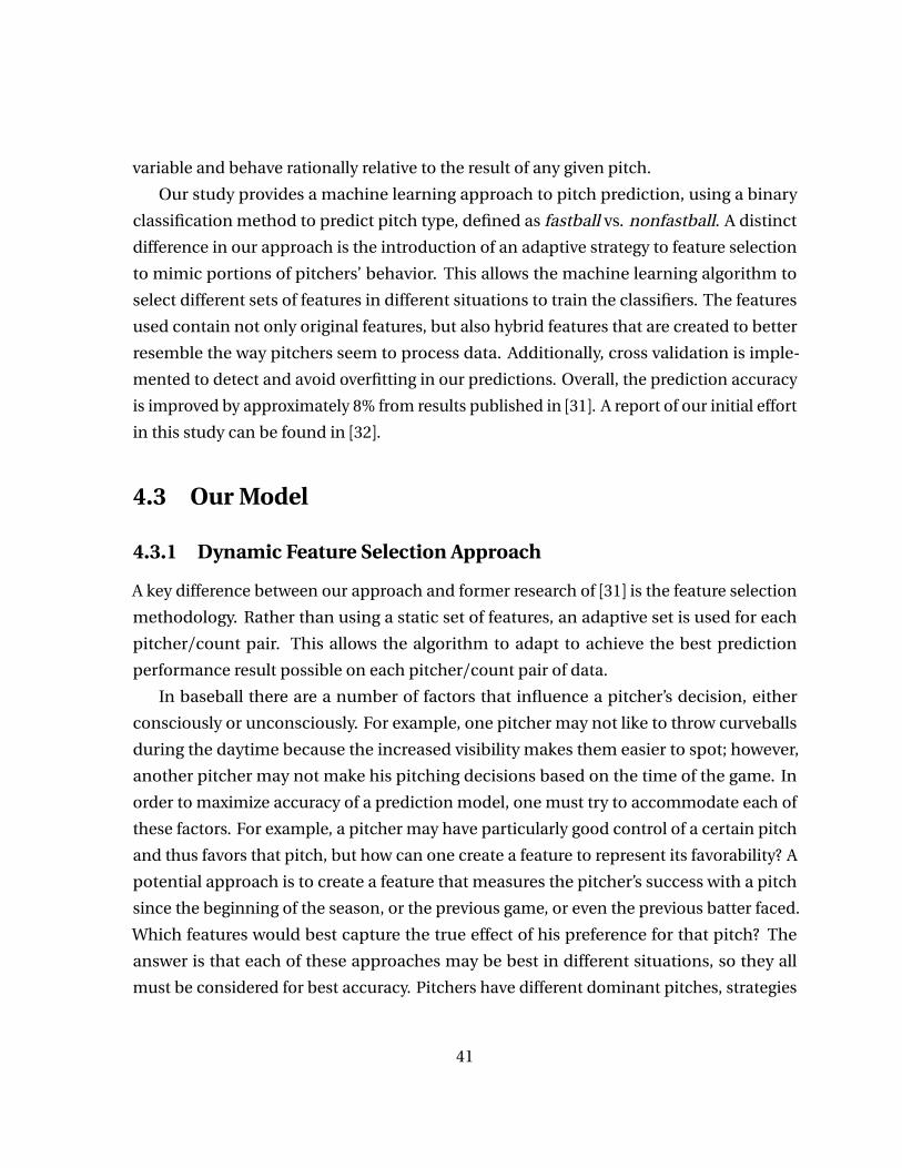
Figure 4.1 Distribution of Group 1 features (1-13) via feature selection methodof Miguel Batista (2008-2009). . . . . . . . . . . . . . . . . . . . . . . . . . . . . 43

viii

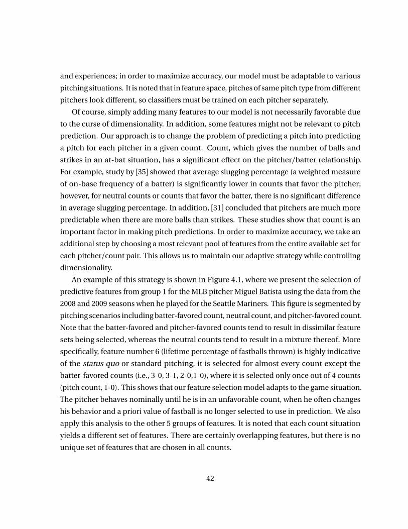
Figure 4.2 Schematic diagram of the proposed adaptive feature selection. . . . . 44Figure 4.3 ROC curve. In this example, three features are measured with the

ROC curve. The blue curve represents the best feature among thethree since it has the highest AUC. The diagonal line represents ran-dom guessing. The area between a ROC curve and the diagonal linequantifies how much better that feature is at distinguishing the twoclasses compared to random guessing. . . . . . . . . . . . . . . . . . . . . . . 45

Figure 4.4 Hypotheis testing for feature selection. The black bars are the numberof features returned by the ROC curve test, the blue are the featuresconsidered optimal for α= .01, the red are for α= 0.05. . . . . . . . . . . 46

Figure 4.5 Prediction accuracy comparison (percents). Symbol: k -Nearest Neigh-bors (k -NN), Support Vector Machine with linear kernel (SVM-L),and with Gaussian kernel (SVM-G), Linear Discriminant Analysis(LDA), Prediction Tree (PT). . . . . . . . . . . . . . . . . . . . . . . . . . . . . . . 48

Figure 4.6 Prediction accuracy by count. . . . . . . . . . . . . . . . . . . . . . . . . . . . . 49

Figure 5.1 Hepatitis C classification comparison with 10-fold CV over N = 500repetitions. . . . . . . . . . . . . . . . . . . . . . . . . . . . . . . . . . . . . . . . . . . 58

Figure 5.2 Schematic diagram of the proposed diagnosis classification . . . . . . 61Figure 5.3 Parameter Optimization via Grid Search on Hepatitis C (10-CV). . . . 65Figure 5.4 G-Mean comparison on Hepatitis C dataset with 10-fold CV over

N = 500 repetitions. . . . . . . . . . . . . . . . . . . . . . . . . . . . . . . . . . . . . 67Figure 5.5 ROC-AUC comparison on Hepatitis C dataset with 10-fold CV over

N = 500 repetitions. . . . . . . . . . . . . . . . . . . . . . . . . . . . . . . . . . . . . 68Figure 5.6 Feature Selection comparison with 10-fold CV over N = 500 repeti-

tions. Number of missing values associated with features 19, 16, 20are 67, 29, and 20 respectively (see Table 5.3). . . . . . . . . . . . . . . . . . 70

Figure 5.7 The scatter plots of the reduced feature subsets by LFDA. . . . . . . . . 71

Figure 6.1 Relationship among three main components of this learning model. 74

ix

CHAPTER

1

INTRODUCTION

1.1 Statement of the Problems

In this thesis, we address some challenges in supervised learning when dealing with both

large and small datasets in the context of baseball pitch prediction and medical diagnosis

domains. The purpose of this dissertation is to address some major issues that come up

with each problem. For pitch prediction, the challenge is finding better alternatives for

pitch prediction when only pre-pitch information is available in training. Furthermore,

pitchers tend to develop similar pitching patterns at the same pitch count. So instead of

having one learning model per pitcher, having a separate model for each pitcher-count

pair may adapt to the changes in game situation better. This further data segmentation

indeed divides the number of observations available for training classifier into smaller sets.

This brings us back to the previous challenge, how to find features with higher predictive

strength to compensate for the potential lack of training data. We propose in this thesis an

1

approach that will overcome this shortcoming. More specifically, from the raw data, we

generate synthetic features that replicate human (pitchers) decision making, then group

them in their similarity and perform two filtering steps to include only a set of optimal

features that are then used for training classifiers. In validation, we applied our final model

to other datasets that were unseen by the machine to ensure its effectiveness in predicting

future data.

For Hepatitis C diagnosis, researchers have been developing methods for disease classi-

fication where nearly perfect (above 95%) accuracy were reached. Many of these studies

however omit the presence of class imbalance where accuracy alone is a poor evalua-

tion metric. Some studies use validation method, but report only the best result, another

misleading measurement of classification performance with particularly small number

of training observations. We propose a method that (1) provides a simpler solution that

outperforms the current methods and (2) employs parameters optimization and cross

validation within metrics designated for treating class imbalance.

The essence of our methods is to attain the best fit of the (in-sample) data at hand

and perform reliably with the out-of-sample data once they encountered (i.e., minimize

overfitting possibilities). To achieve this goal, we carefully examine theoretical foundation of

overfitting, modify our classifier appropriately and provide as much theoretical justification

to the observed heuristic as possible.

1.2 Dissertation Outline

The thesis begins, in Chapter 2, with an introduction of the supervised learning and three

classification techniques used later in this study. Chapter 3 follows with the discussion of

the overfitting problem in supervised learning, as well as two useful tools to address the

overfitting problem. In Chapter 4 we propose a pitch prediction model, built on PITCHf/x

data of MLB seasons 2008-2012. We also compare the performance of various classification

methods mentioned and employ cross validation techniques that previously introduced

in Chapter 2 and 3. Chapter 5 focuses on the medical diagnosis applications in which

we reconfigure the Support Vector Machine classification with weighted cost and employ

parameters optimization and conduct a wide range of validation techniques to address

2

the overfitting and to enhance the performance overall. Chapter 6 draws conclusions and

suggests areas of potential interest for future work.

1.3 Summary of Contributions

This section summarizes the contributions of this study and refers to the specific sections

of the thesis where they can be found:

1. We design and implement a novel feature selection approach for baseball pitch

prediction (section 4.3). Our model is shown to adapt well to the different pitchers

(section 4.4.3) and different count situation (section 4.4.2) even at the time they

change their pitch type. Overall, our experimental results show that our model (1)

can achieve higher accuracy (up to 10 %) than the existing method under hold-out

validation (introduced in section 3.2.1) and (2) shown to be stable with low variances

in cross validation results (less than 2% difference).

2. We propose a new disease diagnosis system that is able to combat overfitting caused by

unbalanced datasets. Our model adapts the Support Vector Machine (SVM) method

using modified cost function that is sensitive to class imbalance (section 5.3.2). We

implement cross validation within the grid search algorithm to determine the best

choices of parameters C and γ of the SVM with Gaussian kernel (section 5.3.3). For

each classifier, we make 500 simulation runs to measure and compare consistency in

term of variances.

3

CHAPTER

2

CLASSIFICATION

Classification is the process of taking an unlabeled data observation and using some rule

or decision-making process to assign a label to it. GivenX is the input space and Y is

the output space (often called labels), D denotes the data set of input-output examples

(x1, y1), ...(xN , yN )where yi = f (xi ) for i = 1, ..., N . The process of classification is to find an

algorithm or strategy that uses the data setD to find a function g from the hypothesis set

H that best approximates the ideal function f :X →Y [1].To support this concept, in [1], the authors present the credit card approval example.

The goal here is for the bank to use historical records of previous customers to figure

out a good formula for credit approval. In this case, as illustrated in Figure 2.1, xi is the

customer information that is used to make a credit decision, yi is a Yes/No decision, f is

the ideal formula for credit approval and data set D contains all input-output examples

corresponding to previous customers and the credit decision for them in hindsight. Once

we find g ( f remains unknown) that best matches f on the training data, we apply g to

classify new credit card customer with the hope that it would still match f on (future)

4

UNKNOWN TARGET FUNCTIONf :X →Y

TRAINING EXAMPLES(x1, y1), · · · , (xN , yN )

LEARNINGALGORITHM

A

HYPOTHESISg ≈ f

HYPOTHESIS SETH

Figure 2.1: Basic setup of the learning problem [1]

5

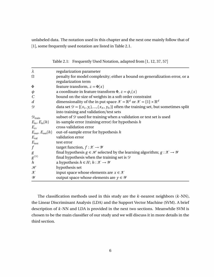
unlabeled data. The notation used in this chapter and the next one mainly follow that of

[1], some frequently used notation are listed in Table 2.1.

Table 2.1: Frequently Used Notation, adapted from [1, 12, 37, 57]

λ regularization parameterΩ penalty for model complexity; either a bound on generalization error, or a

regularization termΦ feature transform, z =Φ(x )φ a coordinate in feature transform Φ, z =φi (x )C bound on the size of weights in a soft order constraintd dimensionality of the in put spaceX =Rd orX = 1×Rd

D data setD = (x1, yi ), ..., (xN , yN ) often the training set, but sometimes splitinto training and validation/test sets

Dtrain subset ofD used for training when a validation or test set is usedEin, Ein(h ) in-sample error (training error) for hypothesis hEcv cross validation errorEout, Eout(h ) out-of-sample error for hypothesis hEval validation errorEtest test errorf target function, f :X →Yg final hypothesis g ∈H selected by the learning algorithm; g :X →Yg (D) final hypothesis when the training set isDh a hypothesis h ∈H ; h :X →YH hypothesis setX input space whose elements are x ∈XY output space whose elements are y ∈Y

The classification methods used in this study are the k -nearest neighbors (k -NN),

the Linear Discriminant Analysis (LDA) and the Support Vector Machine (SVM). A brief

description of k -NN and LDA is provided in the next two sections. Meanwhile SVM is

chosen to be the main classifier of our study and we will discuss it in more details in the

third section.

6

2.1 k -Nearest Neighbors

The k -nearest neighbors algorithm (k -NN) classifies an unlabeled point based on the

closest k training points in the multidimensional feature space; each of the k neighbors

has a class label and the label of a given point is determined by the majority vote of the

class labels of its k -nearest neighbors, see [57]. An example of k-NN is presented below in

Figure 2.2.

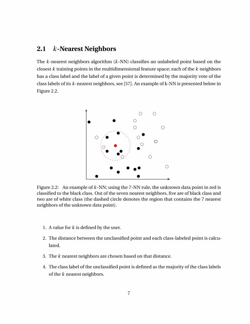
Figure 2.2: An example of k -NN; using the 7-NN rule, the unknown data point in red isclassified to the black class. Out of the seven nearest neighbors, five are of black class andtwo are of white class (the dashed circle denotes the region that contains the 7 nearestneighbors of the unknown data point).

1. A value for k is defined by the user.

2. The distance between the unclassified point and each class-labeled point is calcu-

lated.

3. The k nearest neighbors are chosen based on that distance.

4. The class label of the unclassified point is defined as the majority of the class labels

of the k nearest neighbors.

7

This method is customizable—the user can use different values of k and optionally pick

different distance metrics. The standard choice of metric is the Euclidean distance (2.1),

d Eucl(x , y ) =l∑

i=1

(xi − yi )2. (2.1)

Mahalanobis distance (2.2) takes into account the correlations of the data,

d iMahal(x , y ) =

Æ

(x − y TΣ−1(x − y ), (2.2)

where Σ is the covariance [9, 57]. It is clear that if the covariance matrix Σ is the identity

matrix, then Mahalanobis distance is the same as the Euclidean distance. Another common

metric often used with k -NN is the Manhattan distance (2.3) ,also known as the city-block

distance or L1 norm,

d Man(x , y ) =l∑

i=1

|xi − yi |. (2.3)

An example of a binary class problem using k -NN classifier is presented below. In this

example, data from both classes are generated from the Gaussian distribution with different

means and covariances, as illustrated in Figure 2.3. We use the k -NN algorithm with three

metrics above to classify the unknown data set (black). The unknown set distributes similar

to class 2 but its center is closer to that of class 1. As shown in Table 2.2, Mahalanobis

outperforms the other two types of distance in this case because it pays more attention to

the covariances of each class. However the drawback is the time complexity due to matrix

multiplication.

Table 2.2: Accuracy and speed comparison of k -NN method using different metrics

Methods Accuracy CPU timek-NN 97.80 0.039014s

k-NN Man 97.90 0.039674sk-NN Mahal 98.40 0.174085s

8

x-5 0 5 10

y

-4

-2

0

2

4

6

8

Class 1Class 2unknown

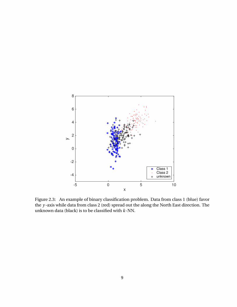
Figure 2.3: An example of binary classification problem. Data from class 1 (blue) favorthe y -axis while data from class 2 (red) spread out the along the North East direction. Theunknown data (black) is to be classified with k -NN.

9

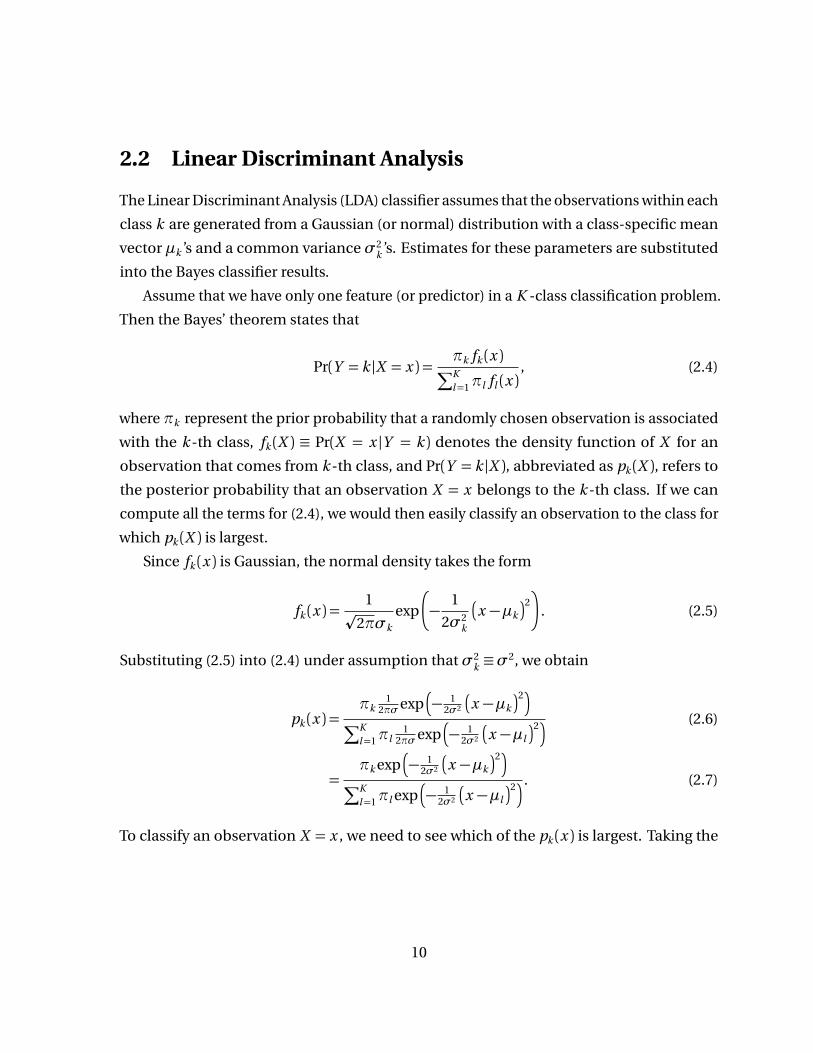
2.2 Linear Discriminant Analysis

The Linear Discriminant Analysis (LDA) classifier assumes that the observations within each

class k are generated from a Gaussian (or normal) distribution with a class-specific mean

vector µk ’s and a common varianceσ2k ’s. Estimates for these parameters are substituted

into the Bayes classifier results.

Assume that we have only one feature (or predictor) in a K -class classification problem.

Then the Bayes’ theorem states that

Pr(Y = k |X = x ) =πk fk (x )

∑Kl=1πl fl (x )

, (2.4)

where πk represent the prior probability that a randomly chosen observation is associated

with the k -th class, fk (X ) ≡ Pr(X = x |Y = k ) denotes the density function of X for an

observation that comes from k -th class, and Pr(Y = k |X ), abbreviated as pk (X ), refers to

the posterior probability that an observation X = x belongs to the k -th class. If we can

compute all the terms for (2.4), we would then easily classify an observation to the class for

which pk (X ) is largest.

Since fk (x ) is Gaussian, the normal density takes the form

fk (x ) =1

p2πσk

exp

−1

2σ2k

x −µk

2

. (2.5)

Substituting (2.5) into (2.4) under assumption thatσ2k ≡σ

2, we obtain

pk (x ) =πk

12πσexp

− 12σ2

x −µk

2

∑Kl=1πl

12πσexp

− 12σ2

x −µl

2 (2.6)

=πk exp

− 12σ2

x −µk

2

∑Kl=1πl exp

− 12σ2

x −µl

2 . (2.7)

To classify an observation X = x , we need to see which of the pk (x ) is largest. Taking the

10

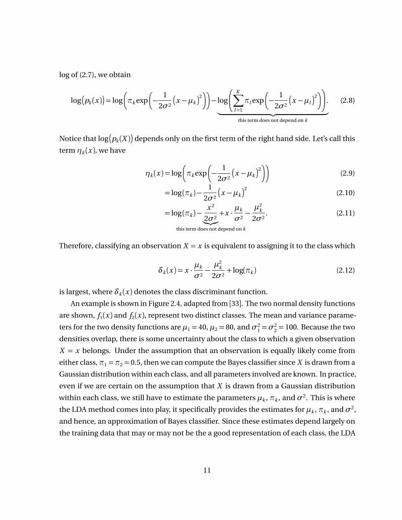
log of (2.7), we obtain

log

pk (x )

= log

πk exp

−1

2σ2

x −µk

2

− log

K∑

l=1

πl exp

−1

2σ2

x −µl

2

.

︸ ︷︷ ︸

this term does not depend on k

(2.8)

Notice that log

pk (X )

depends only on the first term of the right hand side. Let’s call this

term ηk (x ), we have

ηk (x ) = log

πk exp

−1

2σ2

x −µk

2

(2.9)

= log (πk )−1

2σ2

x −µk

2(2.10)

= log (πk )−x 2

2σ2︸︷︷︸

this term does not depend on k

+x ·µk

σ2−µ2

k

2σ2. (2.11)

Therefore, classifying an observation X = x is equivalent to assigning it to the class which

δk (x ) = x ·µk

σ2−µ2

k

2σ2+ log(πk ) (2.12)

is largest, where δk (x ) denotes the class discriminant function.

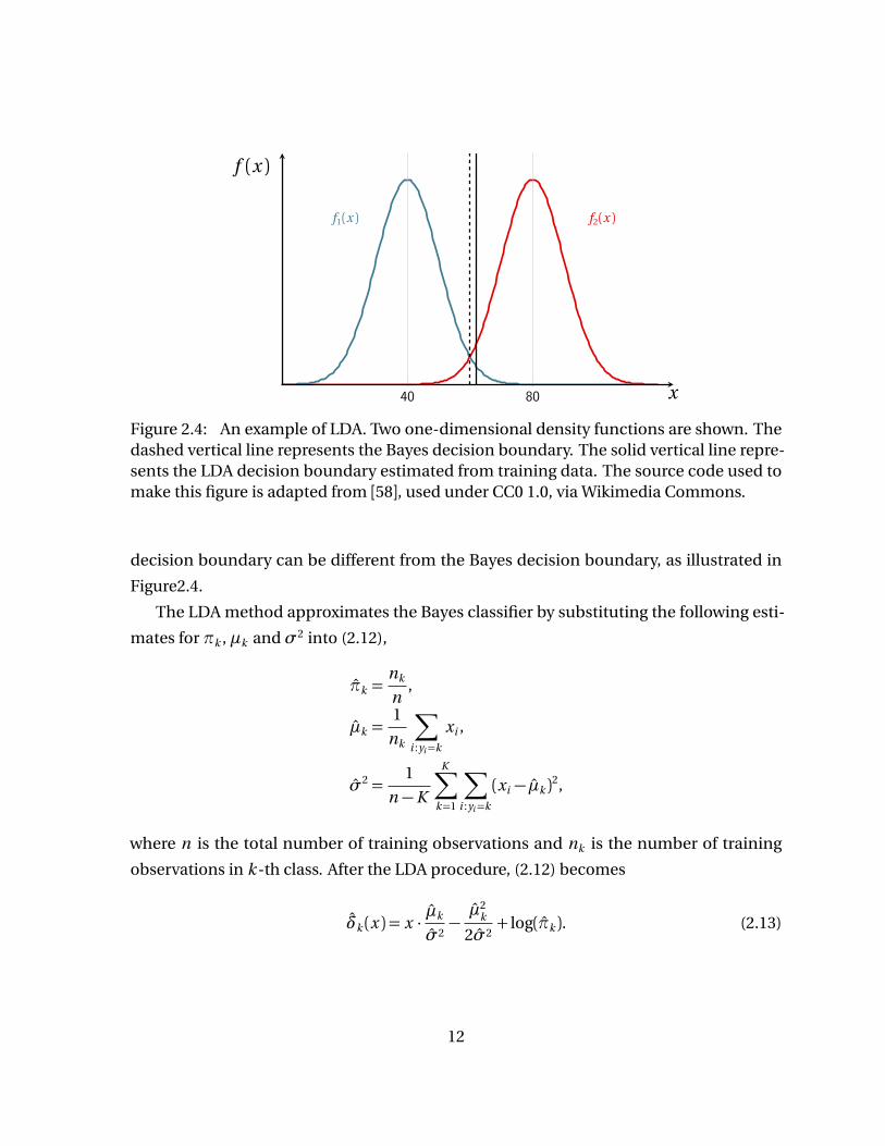
An example is shown in Figure 2.4, adapted from [33]. The two normal density functions

are shown, f1(x ) and f2(x ), represent two distinct classes. The mean and variance parame-

ters for the two density functions are µ1 = 40, µ2 = 80, andσ21 =σ

22 = 100. Because the two

densities overlap, there is some uncertainty about the class to which a given observation

X = x belongs. Under the assumption that an observation is equally likely come from

either class, π1 =π2 = 0.5, then we can compute the Bayes classifier since X is drawn from a

Gaussian distribution within each class, and all parameters involved are known. In practice,

even if we are certain on the assumption that X is drawn from a Gaussian distribution

within each class, we still have to estimate the parameters µk , πk , and σ2. This is where

the LDA method comes into play, it specifically provides the estimates for µk , πk , andσ2,

and hence, an approximation of Bayes classifier. Since these estimates depend largely on

the training data that may or may not be the a good representation of each class, the LDA

11

f2(x )f1(x )

40 80 x

f (x )

Figure 2.4: An example of LDA. Two one-dimensional density functions are shown. Thedashed vertical line represents the Bayes decision boundary. The solid vertical line repre-sents the LDA decision boundary estimated from training data. The source code used tomake this figure is adapted from [58], used under CC0 1.0, via Wikimedia Commons.

decision boundary can be different from the Bayes decision boundary, as illustrated in

Figure2.4.

The LDA method approximates the Bayes classifier by substituting the following esti-

mates for πk , µk andσ2 into (2.12),

πk =nk

n,

µk =1

nk

∑

i :yi=k

xi ,

σ2 =1

n −K

K∑

k=1

∑

i :yi=k

(xi − µk )2,

where n is the total number of training observations and nk is the number of training

observations in k -th class. After the LDA procedure, (2.12) becomes

δk (x ) = x ·µk

σ2−µ2

k

2σ2+ log(πk ). (2.13)

12

The LDA classifier can be extended to multiple predictors. To do this, we assume that

X = (X1, X2, ..., Xp ) is drawn from a multivariate Gaussian distribution with a class-specific

mean vector and common covariance matrix, the corresponding equations (2.5) and (2.12)

are

f (x ) =1

(2π)p/2|Σ|1/2exp

−1

2(x −µ)TΣ−1(x −µ)

, (2.14)

and

δk (x ) = x TΣ−1µk −1

2µT

k Σ−1µk + log(πk ). (2.15)

The formulas for estimating the unknown parameters πk , µk , and Σ are similar to the one-

dimensional case. To assign an observation X = x , the LDA uses these estimates in (2.15)

and assigns the class label for which discrimination function δk (x ) is largest. The word

linear in the classifier’s name comes from the fact that these discrimination functions are

linear functions of x . Unlike the k -NN, where no assumptions are made about the shape

of the decision boundary, the LDA produces linear decision boundaries. See [33] for more

details.

2.3 Support Vector Machines

2.3.1 Linear Separable Case

Support Vector Machine is a linear classification tool that simultaneously optimizes predic-

tion accuracy and avoids overfitting (Chapter 3). The algorithm is dependent on the notion

of margin.

For a two-class classification problem, the separating hyperplane

u (x ) =w · x + b (2.16)

is not unique as it may be biased towards one class 1. The goal is to maximize the distance

between two classes, and effectively drawing the decision boundary that maximizes this

margin. Intuitively, this separation is achieved by the hyperplane that has the largest

distance to the nearest training data point (the so-called support vectors) of either class.

1the dot symbol in (2.16) denotes the inner product

13

w· x+ b=

0w· x+ b=

1

w· x+ b=−1

2||w ||

|b |||w ||

w

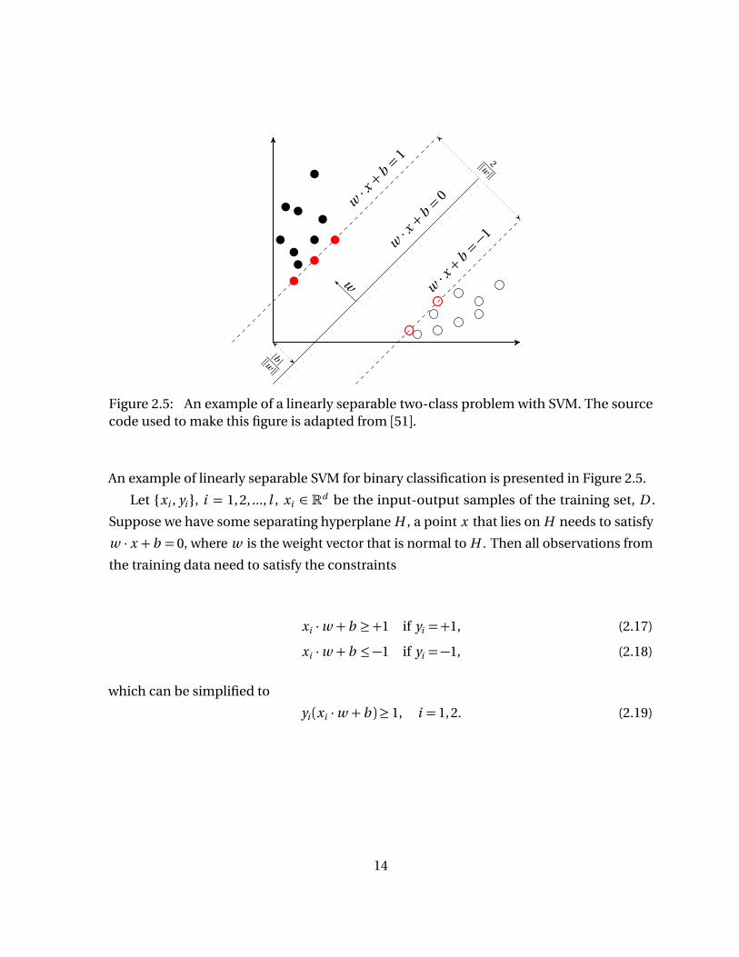
Figure 2.5: An example of a linearly separable two-class problem with SVM. The sourcecode used to make this figure is adapted from [51].

An example of linearly separable SVM for binary classification is presented in Figure 2.5.

Let xi , yi , i = 1,2, ..., l , xi ∈ Rd be the input-output samples of the training set, D .

Suppose we have some separating hyperplane H , a point x that lies on H needs to satisfy

w · x + b = 0, where w is the weight vector that is normal to H . Then all observations from

the training data need to satisfy the constraints

xi ·w + b ≥+1 if yi =+1, (2.17)

xi ·w + b ≤−1 if yi =−1, (2.18)

which can be simplified to

yi (xi ·w + b )≥ 1, i = 1, 2. (2.19)

14

We define the following hyperplanes,

H1 : xi ·w + b =+1,

H2 : xi ·w + b =−1,(2.20)

such that the points on the planes H1 and H2 are the support vectors. Note that H1 and H2

have same normal vector hence they are parallel to each other. In addition, no training

points should lie between them. Now, from (2.20) the distances from the origin to H1 and

H2 are|1− b |||w ||

and| −1− b |||w ||

, respectively. Hence, the margin between H1 and H2 is2

||w ||. In

order to maximize the margin between H1 and H2, ||w ||must be minimized. Combining

this with the constraint (2.19), we have an optimization problem

min1

2||w ||2, (2.21)

subject to yi (xi w + b )≥ 1, i = 1, 2, ..., l . (2.22)

Since the norm ||w || involves a square root, which makes optimization difficult, we have

replaced ||w || with||w ||2

2. We now have a quadratic program that can be solved using

Lagrange multipliers, as suggested in [14, 57, 60]. The Lagrangian for this problem is

L =1

2||w ||2−

l∑

i=1

αi [yi (xi ·w + b )−1], (2.23)

where αi denotes the Lagrangian multipliers. To minimize L , the following Karush-Kuhn-

Tucker (KKT) conditions [57]must be satisfied

Lw = 0, (2.24)

Lb = 0, (2.25)

αi ≥ 0, i = 1, 2, ..., l , (2.26)

αi [yi (xi ·w + b )−1] = 0, i = 1, 2, ..., l . (2.27)

15

Combining these with equation (2.23) we have

w =l∑

i=1

αi yi xi , (2.28)

l∑

i=1

αi yi = 0. (2.29)

We now consider the Lagrangian duality problem which is called the Wolfe dual repre-

sentation form. Following [14, 57], we have,

max1

2||w ||2−

l∑

i=1

αi [yi (xi ·w + b )−1], (2.30)

subject to w =l∑

i=1

αi yi xi , (2.31)

l∑

i=1

αi yi = 0, (2.32)

αi ≥ 0. (2.33)

Substituting (2.31) in (2.30) yields

1

2

l∑

i=1

αi yi xi

·

l∑

j=1

α j yj x j

!

−

l∑

i=1

αi yi xi

·

l∑

j=1

α j yj x j

!

+ bl∑

i=1

αi yi −l∑

i=1

αi

!

. (2.34)

Applying (2.32) and rearranging the terms, we have

l∑

i=1

αi −1

2

l∑

i=1

αi yi xi

·

l∑

j=1

α j yj x j

!

. (2.35)

16

The Lagrangian problem becomes

maxl∑

i=1

αi −1

2

∑

i , j=1

αiα j yi yj xi · x j , (2.36)

subject tol∑

i=1

αi yi = 0, (2.37)

αi ≥ 0. (2.38)

Ifαi > 0, the corresponding data point is the support vector and the solution for the optimal

separating hyperplane is

w =n∑

i=1

αi yi xi , (2.39)

where n ≤ l is the number of support vectors. Once we determine w and b , from equation

(2.27), the optimal linear discriminant function is

g (x ) = sgn(w · x + b ) (2.40)

= sgn

l∑

i=1

αi yi xi · x + b

. (2.41)

Finally, from equation (2.27), for any nonzero αm which is associated with some support

17

vector xm and label ym , we compute b as followed

αm [ym (xm ·w + b )−1] = 0, (2.42)

ym (xm ·w + b )−1= 0, (2.43)

ym xm ·w + ym b −1= 0, (2.44)

b =1

ym(1− ym xm w ), (2.45)

=1

ym− xm ·w , (2.46)

=1

ym−

l∑

i=1

αi yi xi · xm , (2.47)

= ym −l∑

i=1

αi yi xi · xm . (2.48)

Notice that equation (2.48) holds because ym =±1.

2.3.2 Nonseparable Case - Soft Margin SVM

The above setup only works for separable data. For a nonseparable two-class problem, we

cannot draw a separating hyperplane with associated hyperplanes H1 and H2 such that

there is no data point lying between them. To address this issue, recall that H1 and H2 have

the form

xi ·w + b =±1 (2.49)

and the margin is the distance between them. Any training data point, xi (with associated

class label yi ) in the training set must belong to one of the following three cases (see Figure

2.6),

• xi lies outside the margin and correctly classified, so x satisfies the inequality con-

straints in (2.22), i.e., yi (xi ·w + b )≥ 1,

• xi lies between the margin and correctly classified, so 0≤ yi (xi ·w + b )< 1,

• xi lies between the margin and incorrectly classified, so yi (xi ·w + b )< 0.

18

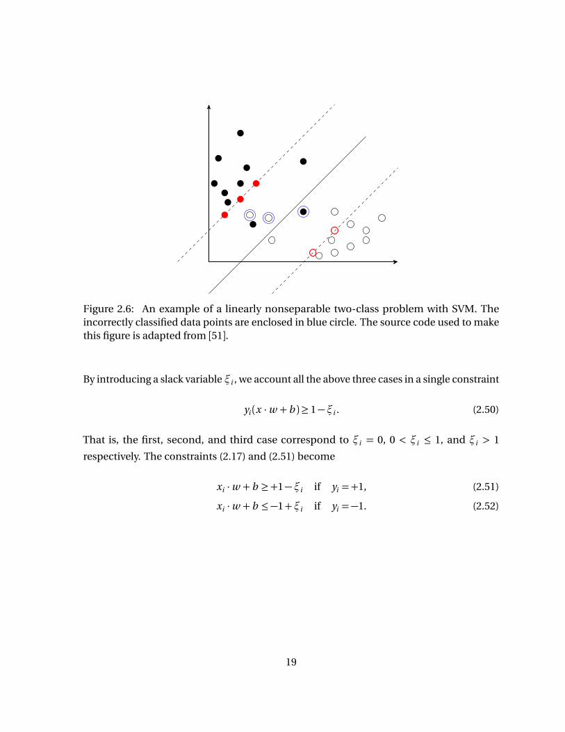
Figure 2.6: An example of a linearly nonseparable two-class problem with SVM. Theincorrectly classified data points are enclosed in blue circle. The source code used to makethis figure is adapted from [51].

By introducing a slack variable ξi , we account all the above three cases in a single constraint

yi (x ·w + b )≥ 1−ξi . (2.50)

That is, the first, second, and third case correspond to ξi = 0, 0 < ξi ≤ 1, and ξi > 1

respectively. The constraints (2.17) and (2.51) become

xi ·w + b ≥+1−ξi if yi =+1, (2.51)

xi ·w + b ≤−1+ξi if yi =−1. (2.52)

19

The new optimization problem is

min1

2||w ||2+C

l∑

i=1

ξi ,

subject to yi (xi w + b )≥ 1−ξi , i = 1, 2, ..., l ,

ξi ≥ 0, i = 1, 2, ..., l ,

(2.53)

where C is a parameter that controls the trade-off between the two main goals: maximizing

margin and having fewer number of misclassification. This is still a convex optimization

problem, hence we proceed with the Lagrange method as before [57]. The Lagrangian for

this new problem is

L =1

2||w ||2+C

l∑

i=1

ξi −l∑

i=1

µiξi −l∑

i=1

αi [yi (xi ·w + b )−1+ξi ], (2.54)

with the corresponding KKT conditions

Lw = 0 or w =l∑

i=1

αi yi xi , (2.55)

Lb = 0 orl∑

i=1

αi yi = 0, (2.56)

Lξi= 0 or C −µi −αi = 0, i = 1, 2, ..., l , (2.57)

αi [yi (xi ·w + b )−1+ξi ] = 0, i = 1, 2, ..., l , (2.58)

µiξi = 0, i = 1, 2, ..., l , (2.59)

αi ≥ 0, i = 1, 2, ..., l , (2.60)

µi ≥ 0, i = 1, 2, ..., l , (2.61)

20

and the associated Wolfe dual representation

max1

2||w ||2+C

l∑

i=1

ξi −l∑

i=1

µiξi −l∑

i=1

αi [yi (xi ·w + b )−1+ξi ], (2.62)

subject to w =l∑

i=1

αi yi xi , (2.63)

l∑

i=1

αi yi = 0, (2.64)

C −µi −αi = 0, i = 1, 2, ..., l , (2.65)

αi ≥ 0, µi ≥ 0, i = 1, 2, ..., l . (2.66)

By substituting the equality constraints (2.63) and (2.64) into the Lagrangian (2.62), the

optimization problem becomes

maxl∑

i=1

αi −1

2

∑

i , j=1

αiα j yi yj xi · x j , (2.67)

subject tol∑

i=1

αi yi = 0, (2.68)

0≤αi ≤C , i = 1, 2, ..., l . (2.69)

As before, we use KKT conditions, equations (2.58) and (2.59) to solve for b . Combining

equation (2.57), C −αi −µi = 0 and equation (2.59), µiξi = 0 in show that ξi = 0 if αi <C .

Therefore we simply take any point that satisfies 0<αi <C and ξi = 0, and using equation

(2.58) to compute b . With some algebra, we should obtain the solution for b that is identical

to equation (2.48) from the separable case in the previous section. Once α, w , and b are

determined, we obtain the optimal decision function

g (x ) = sgn

l∑

i=1

αi yi xi · x + b

, (2.70)

where b = ym −l∑

i=1

αi yi xi · xm . (2.71)

21

This decision function is identical to equation (2.41) of the separable case with the only

exception that the Lagrange multipliers αi are now bounded above by C , as seen in (2.69)

[14].

2.3.3 Nonlinearly Separable Case - Kernel trick

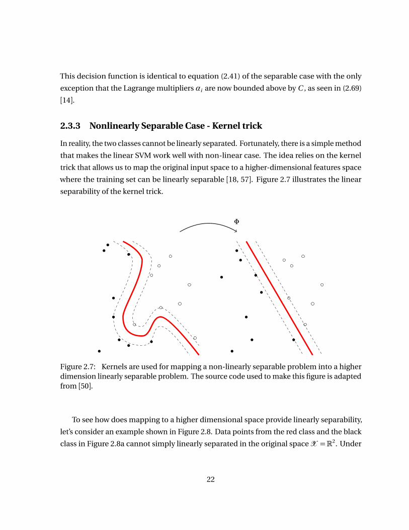
In reality, the two classes cannot be linearly separated. Fortunately, there is a simple method

that makes the linear SVM work well with non-linear case. The idea relies on the kernel

trick that allows us to map the original input space to a higher-dimensional features space

where the training set can be linearly separable [18, 57]. Figure 2.7 illustrates the linear

separability of the kernel trick.

Φ

Figure 2.7: Kernels are used for mapping a non-linearly separable problem into a higherdimension linearly separable problem. The source code used to make this figure is adaptedfrom [50].

To see how does mapping to a higher dimensional space provide linearly separability,

let’s consider an example shown in Figure 2.8. Data points from the red class and the black

class in Figure 2.8a cannot simply linearly separated in the original spaceX =R2. Under

22

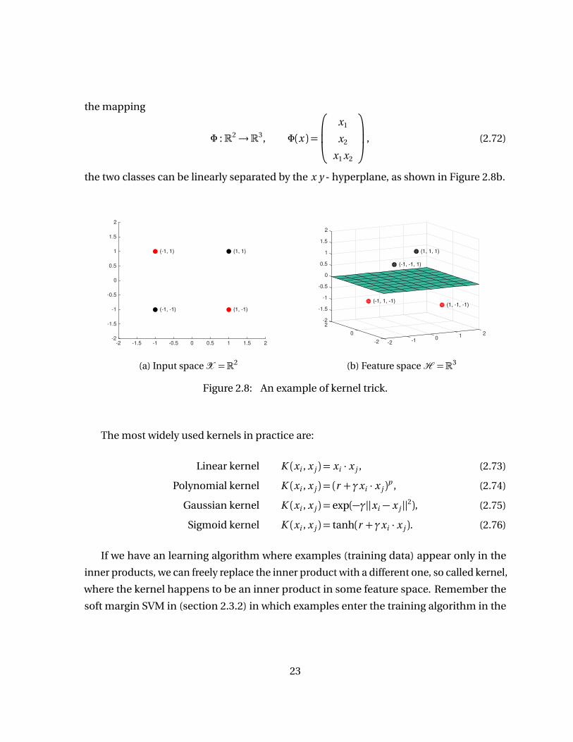
the mapping

Φ :R2→R3, Φ(x ) =

x1

x2

x1 x2

, (2.72)

the two classes can be linearly separated by the x y - hyperplane, as shown in Figure 2.8b.

-2 -1.5 -1 -0.5 0 0.5 1 1.5 2-2

-1.5

-1

-0.5

0

0.5

1

1.5

2

(1, 1)

(-1, -1)

(-1, 1)

(1, -1)

(a) Input spaceX =R2

2

(1, -1, -1)

1

(1, 1, 1)

0

(-1, -1, 1)

-1

(-1, 1, -1)

-2-2

0

2

1.5

1

0.5

0

-0.5

-1

-1.5

-22

(b) Feature spaceH =R3

Figure 2.8: An example of kernel trick.

The most widely used kernels in practice are:

Linear kernel K (xi , x j ) = xi · x j , (2.73)

Polynomial kernel K (xi , x j ) = (r +γxi · x j )p , (2.74)

Gaussian kernel K (xi , x j ) = exp(−γ||xi − x j ||2), (2.75)

Sigmoid kernel K (xi , x j ) = tanh(r +γxi · x j ). (2.76)

If we have an learning algorithm where examples (training data) appear only in the

inner products, we can freely replace the inner product with a different one, so called kernel,

where the kernel happens to be an inner product in some feature space. Remember the

soft margin SVM in (section 2.3.2) in which examples enter the training algorithm in the

23

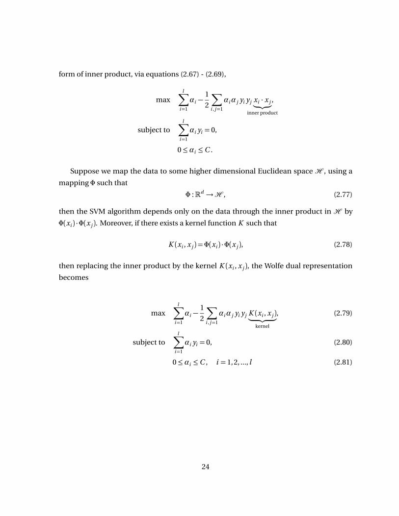
form of inner product, via equations (2.67) - (2.69),

maxl∑

i=1

αi −1

2

∑

i , j=1

αiα j yi yj xi · x j︸ ︷︷ ︸

inner product

,

subject tol∑

i=1

αi yi = 0,

0≤αi ≤C .

Suppose we map the data to some higher dimensional Euclidean spaceH , using a

mapping Φ such that

Φ :Rd →H , (2.77)

then the SVM algorithm depends only on the data through the inner product inH by

Φ(xi ) ·Φ(x j ). Moreover, if there exists a kernel function K such that

K (xi , x j ) =Φ(xi ) ·Φ(x j ), (2.78)

then replacing the inner product by the kernel K (xi , x j ), the Wolfe dual representation

becomes

maxl∑

i=1

αi −1

2

∑

i , j=1

αiα j yi yj K (xi , x j )︸ ︷︷ ︸

kernel

, (2.79)

subject tol∑

i=1

αi yi = 0, (2.80)

0≤αi ≤C , i = 1, 2, ..., l (2.81)

24

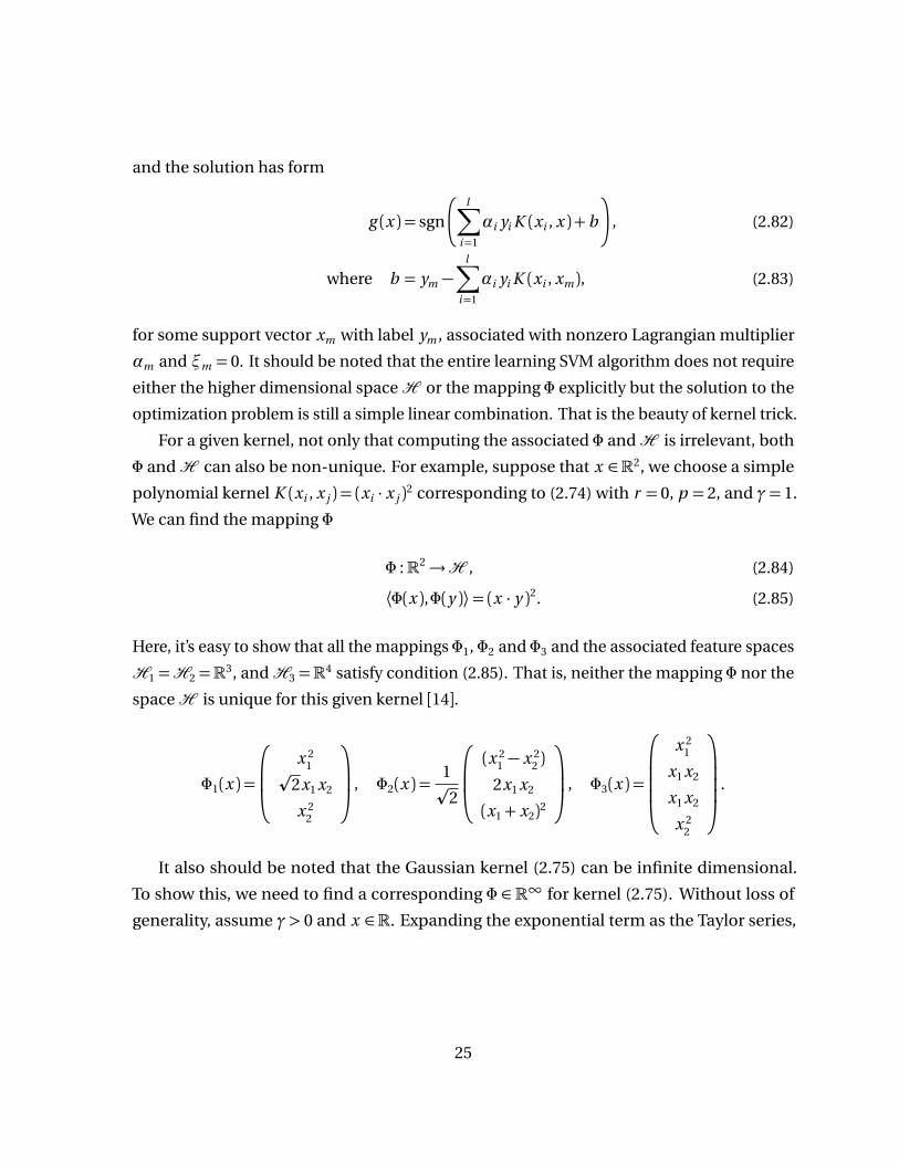
and the solution has form

g (x ) = sgn

l∑

i=1

αi yi K (xi , x ) + b

, (2.82)

where b = ym −l∑

i=1

αi yi K (xi , xm ), (2.83)

for some support vector xm with label ym , associated with nonzero Lagrangian multiplier

αm and ξm = 0. It should be noted that the entire learning SVM algorithm does not require

either the higher dimensional spaceH or the mapping Φ explicitly but the solution to the

optimization problem is still a simple linear combination. That is the beauty of kernel trick.

For a given kernel, not only that computing the associated Φ andH is irrelevant, both

Φ andH can also be non-unique. For example, suppose that x ∈R2, we choose a simple

polynomial kernel K (xi , x j ) = (xi · x j )2 corresponding to (2.74) with r = 0, p = 2, and γ= 1.

We can find the mapping Φ

Φ :R2→H , (2.84)

⟨Φ(x ),Φ(y )⟩= (x · y )2. (2.85)

Here, it’s easy to show that all the mappings Φ1, Φ2 and Φ3 and the associated feature spaces

H1 =H2 =R3, andH3 =R4 satisfy condition (2.85). That is, neither the mapping Φ nor the

spaceH is unique for this given kernel [14].

Φ1(x ) =

x 21p

2x1 x2

x 22

, Φ2(x ) =

1p

2

(x 21 − x 2

2 )

2x1 x2

(x1+ x2)2

, Φ3(x ) =

x 21

x1 x2

x1 x2

x 22

.

It also should be noted that the Gaussian kernel (2.75) can be infinite dimensional.

To show this, we need to find a corresponding Φ ∈ R∞ for kernel (2.75). Without loss of

generality, assume γ > 0 and x ∈R. Expanding the exponential term as the Taylor series,

25

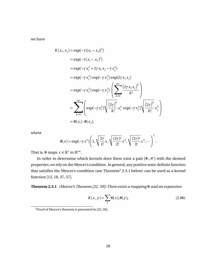
we have

K (xi , x j ) = exp(−γ||xi − x j ||2)

= exp(−γ(xi − x j )2)

= exp(−γx 2i +2γxi x j −γx 2

j )

= exp(−γx 2i ) exp(−γx 2

j ) exp(2γxi x j )

= exp(−γx 2i ) exp(−γx 2

j )

∞∑

k=0

2γxi x j

k

k !

=

∞∑

k=0

exp(−γx 2i )

√

√

√

2γk

k !x k

i exp(−γx 2j )

√

√

√

2γk

k !x k

j

=Φ(xi ) ·Φ(x j ),

where

Φ(x ) = exp(−γx 2)

1,

√

√2γ

1!x ,

√

√ (2γ)2

2!x 2,

√

√ (2γ)3

3!x 3, · · ·

T

.

That is, Φmaps x ∈R1 to R∞.

In order to determine which kernels does there exist a pair (Φ,H ) with the desired

properties, we rely on the Mercer’s condition. In general, any positive semi-definite function

that satisfies the Mercer’s condition (see Theorem2 2.3.1 below) can be used as a kernel

function [12, 18, 37, 57].

Theorem 2.3.1 (Mercer’s Theorem [22, 59]) There exists a mapping Φ and an expansion

K (x , y ) =∑

i

Φ(x )iΦ(y )i (2.86)

2Proof of Mercer’s theorem is presented in [22, 59].

26

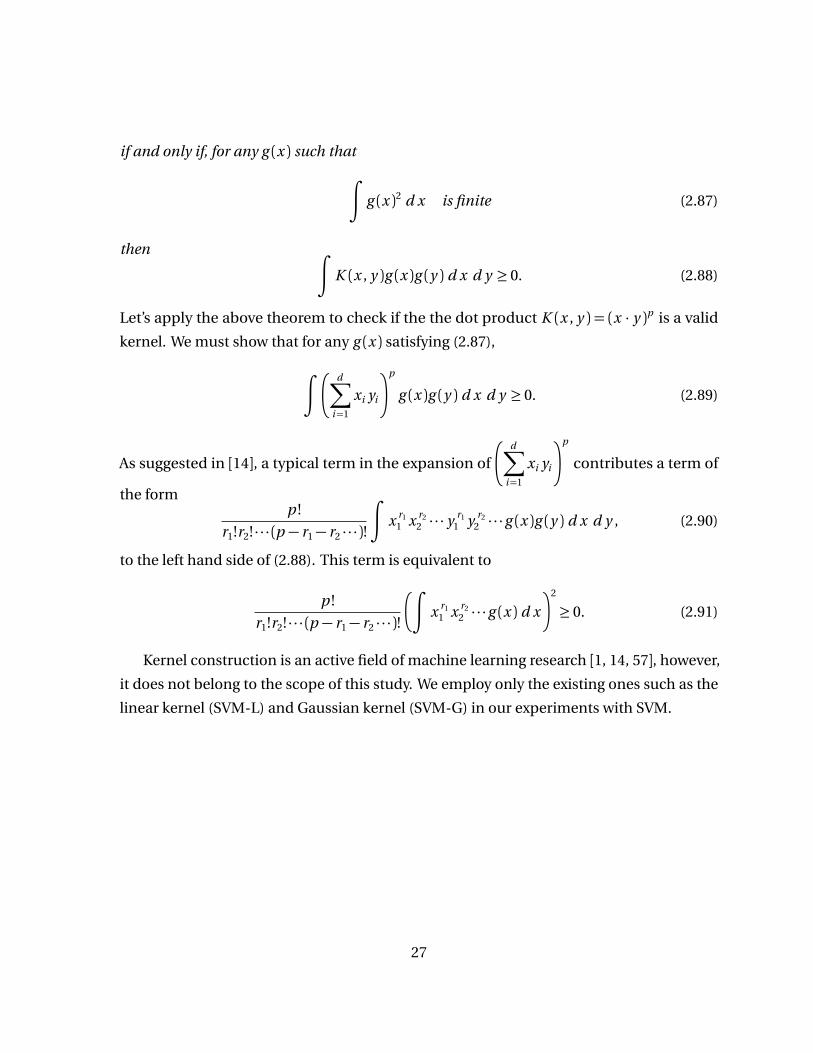
if and only if, for any g (x ) such that

∫

g (x )2 d x is finite (2.87)

then∫

K (x , y )g (x )g (y ) d x d y ≥ 0. (2.88)

Let’s apply the above theorem to check if the the dot product K (x , y ) = (x · y )p is a valid

kernel. We must show that for any g (x ) satisfying (2.87),

∫

d∑

i=1

xi yi

p

g (x )g (y ) d x d y ≥ 0. (2.89)

As suggested in [14], a typical term in the expansion of

d∑

i=1

xi yi

p

contributes a term of

the formp !

r1!r2! · · · (p − r1− r2 · · · )!

∫

x r11 x r2

2 · · · yr1

1 y r22 · · ·g (x )g (y ) d x d y , (2.90)

to the left hand side of (2.88). This term is equivalent to

p !

r1!r2! · · · (p − r1− r2 · · · )!

∫

x r11 x r2

2 · · ·g (x ) d x

2

≥ 0. (2.91)

Kernel construction is an active field of machine learning research [1, 14, 57], however,

it does not belong to the scope of this study. We employ only the existing ones such as the

linear kernel (SVM-L) and Gaussian kernel (SVM-G) in our experiments with SVM.

27

CHAPTER

3

OVERFITTING

Overfitting is the phenomenon where a hypothesis with lower in-sample error Ein yields

a higher out-of-sample error Eout. In this case, Ein is no longer useful in choosing the

hypothesis that best represents the target function. Often it is the case when the model

is more complex than necessary, as Abu-Mostafa (2012) put, "it uses additional degrees

of freedom to fit idiosyncrasies (noise), yielding a final hypothesis that is inferior" [1].

An example of overfitting is illustrated in Figure 3.1. Overfitting can also occurs when a

hypothesis that is far simpler than the target function, hence it is referred as underfitting 1.

Overfitting mainly depends on the three parameters: the noiseσ2, the target function

complexity Q f , and the number of training data points N . Asσ2 increases, more stochastic

noise2 is added to the data. Meanwhile, as Q f increases, we add more deterministic noise3 to

1We will examine this special case in detail in chapter 52When learning from data, there are random fluctuations and/or measurements errors in the data which

cannot be modeled. This phenomenon is referred to the stochastic noise.3For a given learning problem, there is a best approximation to the target function, the part of the target

function outside this best fit acts like noise in the data. This model’s inability to approximate f is referred to

28

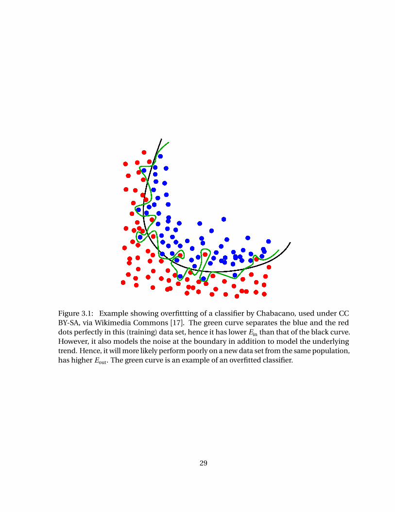
Figure 3.1: Example showing overfittting of a classifier by Chabacano, used under CCBY-SA, via Wikimedia Commons [17]. The green curve separates the blue and the reddots perfectly in this (training) data set, hence it has lower Ein than that of the black curve.However, it also models the noise at the boundary in addition to model the underlyingtrend. Hence, it will more likely perform poorly on a new data set from the same population,has higher Eout. The green curve is an example of an overfitted classifier.

29

the data. As the number of data points N increases, noise levelσ2 drops and less overfitting

occurs. It is important to realize that both stochastic and deterministic noises cannot be

modeled and cannot be distinguished [1]. To understand how these two types of noise

affect the model performance, one could use the bias-variance decomposition of error

(loss) function:

ED [Eout] =σ2+bias+var. (3.1)

In equation (3.1),σ2 and bias are the direct impact of the stochastic noise and deterministic

noise, respectively. The interesting var term is indirectly impacted by both types of the

noise, through the hypothesis setH . Because var is controlled by the size ofH , it decreases

as the number of data points N increases. Moreover, if we makeH more complex, we will

decrease bias in the expense of increasing var. In practice, the later usually dominates, so

overfitting occurs not because of the direct impact on noise, but mainly because of the

indirect impact on variance. In this chapter, we mainly adapt the context of Chapter 4 in

[1]which gives a throughout discussion to the topic of overfitting and the methodology to

prevent overfitting.

3.1 Regularization

Regularization is used to prevent overfitting by explicitly controlling the model complexity.

To achieve this goal, an additional parameter Ω(h ) is introduced to account for model

complexity of an individual hypothesis h . As shown in the error function (3.2), instead of

minimizing Ein(h ) alone, one would minimizes both Ein(h ) and Ω(h ). By doing this, the

learning algorithm is constrained to not only fitting the data well but also using a simpler

hypothesis hence improves generalization [1, 12].

Eout(h )≤ Ein(h ) +Ω(H ) for all h ∈H . (3.2)

Several regularization techniques have been presented in the machine learning litera-

ture. Some notable ones are weight decay [1], L1 and L2 regularization in regression [48],

and Tikhonov regularization [12]. We emphasize on the last technique, most commonly

the deterministic noise.

30

used for ill-posed problems and widely adapted in statistics and machine learning. For ex-

ample, the author of [11] proves that training with noise is equivalent to solving a Tikhonov

regularization with Neural Network classifier. We will also see how it can be viewed as a

soft constraint SVM problem.

In the simplest case, given a mapping A : X → Y , to obtain a regularized solution to

Ax = y , we seek for x that fits y in the least squares sense, but penalize solutions of large

norm and solve the optimization problem

xλ = arg min||Ax − y ||2Y +λ||x ||2X ,

= (A∗A+λI )−1A∗y ,(3.3)

where λ> 0 is called the regularization parameter.

Back to the supervised learning regime, given n input-output examples (x1, y1), ..., (xn , yn )

with xi ∈ Rd and yi ∈ −1,1 for all i , we want to choose a classifier function f :X →Ythat fits the data but not too complex. Tikhonov regularization (3.3) suggests such function

as follows:

minf ∈H

1

n

n∑

i=1

V (yi , f (xi ))+λ|| f ||2H , (3.4)

where V : Y ×Y → R is the loss function, || · ||H is the norm on the hypothesis space

of functionsH , and λ ∈ R is the regularization parameter [55]. The most intuitive loss

function is indeed the missclassifiation loss function, i.e, the 0-1 loss, which gives 0 if we

have classified correctly, f (xi ) and yi have the same sign, and 1 if incorrectly classified. This

forms a step function

V (yi , f (xi )) =

1 for yi f (xi )< 0,

0 for yi f (xi )≥ 0.(3.5)

The major drawback is that the step function (3.5) is non convex (also undefined at

x = 0), which gain difficulties in the optimization problem [1, 55, 57]. To address this

shortcoming, one can use the hinge loss function. In particular, the hinge loss function

assigns a positive loss to correct classification in such 0< yi f (xi )< 1, as shown in Figure

3.2. The goal is to classify most input xi with at least a value of yi f (xi )≥ 1. It’s analogous

31

y*f(x)-3 -2 -1 0 1 2 3

Hin

ge

lo

ss

-1

-0.5

0

0.5

1

1.5

2

2.5

3

3.5

4

Figure 3.2: Hinge loss function. Note that the loss is asymmetric: incorrect classification,yi f (xi )< 0, is linearly increasing loss as yi f (xi ) decreases and correct classification withyi f (xi )≥ 1 is always zero loss.

to the idea of SVM when we want to classifies most of xi outside of the separating margin.

Now, given the hinge-loss function, Tikhonov regularization becomes

minf ∈H

1

n

n∑

i=1

(1− yi f (xi ))++λ|| f ||2H , (3.6)

where (u )+ =maxu , 0. Multiplying (3.6) by1

2λand choosing C =

1

2nλyield

minf ∈H

1

2|| f ||2H +C

n∑

i=1

(1− yi f (xi ))+. (3.7)

Note that the hinge loss is not differentiable at yi f (xi ) = 1. To address this issue, let’s

introduce slack variablesξi such that for each point in the training set,ξi replace (1−yi f (xi ).

32

For each ξi , we require ξi ≥ (1− yi f (xi ))+. The Tikhonov regularization problem becomes

minf ∈H

1

2|| f ||2H +C

n∑

i=1

ξi ,

subject to yi f (xi )≥ 1−ξi , i = 1, ..., n ,

ξi ≥ 0,

(3.8)

which is equivalent to the SVM problem (2.53) in Section 2.3. For a more comprehensive

explanation of regularization perspective on SVM, see [11, 14, 55, 57].

3.2 Validation

In the previous section, we show that regularization can combat overfitting by control

model complexity. Validation on the other hand estimates the out-of-sample error directly,

as illustrated in (3.9). Note that both techniques are often used together in a learning

problem as an attempt to minimizing Eout rather than just Ein.

Eout(h ) = Ein(h ) +overfit penalty︸ ︷︷ ︸

regularization estimates this quantity

,

Eout(h )︸ ︷︷ ︸

validation estimates this quantity

= Ein(h ) +overfit penalty.(3.9)

The process of validation requires the presence of the validation set. But first let’s define the

test set. The test set is a subset of input spaceD that is removed from the data set. The test

set is absolutely not involved in the learning process, hence unlike Ein, Etest is an unbiased

estimation of Eout. The validation set is constructed similarly, it is also a subset ofD that is

not used directly in the training process. However, the validation error, Eval, is used to help

us make certain choices in choosing parameters of a classifier or feature selection. This

indirectly impacts the learning process rendering the validation set no longer qualified

to be a test set. Nevertheless, Eval is still a better choice than Ein in term of bias for model

evaluation.

33

3.2.1 Hold-Out Validation

Hold-out method involves randomly partition the dataset D of size N into two parts: a

training set Dtrain of size (N −K ) and a validation set (or hold out-set) Dval of size K . The

learning model is trained on the Dtrain to obtain a final hypothesis g − that is later used

to predict the responses for the observations in the Dval4. The validation error for g − is

computed using the validation setDval as follows,

Eval =1

K

∑

xn∈Dval

e

g −(xn ), yn

, (3.10)

where e

g −(x ), y

denotes the point-wise error function,

e

g −(x ), y

=

0 for g −(x ) = y ,

1 for otherwise.(3.11)

It is important to realize that the validation error rate Eval gives an unbiased estimate of

Eout because the hypothesis g − was formed independently of the data point inDval. In fact,

taking expectation of Eval with respect toDval, results in

EDval

Eval(g−)

=1

K

∑

xn∈Dval

EDval

e

g −(xn ), yn

, (3.12)

=1

K

∑

xn∈Dval

Exn

e

g −(xn ), yn

, (3.13)

=1

K

∑

xn∈Dval

Eout(g ), (3.14)

= Eout(g−). (3.15)

The first equality in (3.12) uses linearity of expectation and the second equality in (3.13) is

true because e

g −(xn ), yn

depends only on xn . Hold-out method is a very simple strategy

but it has two drawbacks: (1) the test error Eout can be greatly varying depending on which

4The minus subscript in g − indicates that some data points have been removed from the training (forvalidation purpose. At the end g is the final hypothesis that is trained with all data points inDtrain.

34

observations are included in the training and validation set; and (2) only a subset of the

available observations are used for training and validating the model, so we can potentially

lose valuable information especially with smaller datasets [37].

3.2.2 Cross Validation

In the validation process, finding K , the size of the validation set is not easy. The dilemma

we encounter is described in (3.16). In the first approximation, we want K to be small, to

minimize the difference between Eout(g ) and Eout(g −). However, in the second approxima-

tion, larger K results in less variance between Eout(g −) and Eval(g −).

Eout(g ) ≈small K

Eout(g−) ≈

large KEval(g

−) (3.16)

This leads us to a refinement of the hold-out approach, called cross validation (CV), a com-

mon strategy for model selection that gained widespread application due to its simplicity

and universality.

The popularity of the cross validation technique is mostly due to the universality of

the data splitting heuristics [8]. In the basic approach, called k -fold cross-validation, the

original sample is randomly partitioned into k equal size subsamples. Commonly, k = 10 is

considered standard CV, another choice when k =N so K = 1 is referred as leave-one-out

approach. Of the k subsamples, a single subsample is retained as the validation data for

testing the model, and the remaining k − 1 subsamples are used as training data. The

cross-validation process is then repeated k times (the folds), with each of the k subsamples

used exactly once as the validation data. The k results from the folds can then be averaged

(or otherwise combined) to produce a single estimation of the true error rate. That is,

Ecv(g−) =

1

k

k∑

n=1

Eval(g−n ). (3.17)

The advantage of this method is that all observations are used for both training and

validation, and each observation is used for validation exactly once. Not only does k -fold

CV give a nearly unbiased estimate of the generalized (out-of-sample) error rate, it also

reduces the variability in the estimation, hence considered better than the hold-out method

35

in term of avoiding overfitting [37]. However it often produce unpredictable high variability

on small dataset. Efron, Bradley (1983) shows that applying randomized bootstrap (a

nonparametric maximum likelihood estimation) can enhance the stability of regular CV

[27]. Furthermore, Andrew Ng (1996) points out that overfitting can occur even with large

dataset that is partially corrupted by noise. The author shows that it can be overcome

by selecting the hypothesis with a higher CV error, over others with lower CV errors and

propose an algorithm (LOOCVCV 5) to perform this task.

5LOOCVCV: Leave-one-out Cross-Validated Cross Validation

36

CHAPTER

4

BASEBALL PITCH PREDICTION

Baseball, one of the most popular sports in the world, has a uniquely discrete gameplay

structure that naturally allows fans and observers to record information about the game in

progress, resulting in a wealth of data that is available for analysis. Major League Baseball

(MLB), the professional baseball league in the US and Canada, uses a system known as

PITCHf/x to record information about every individual pitch that is thrown in league

play. We apply several machine learning classification methods to this data to classify

pitches by type (fastball or nonfastball). We then extend the classification to prediction by

restricting our analysis to pre-pitch features. By performing significant feature analysis

and introducing a dynamic approach for feature selection, moderate improvement over

published results is achieved.

37

4.1 PITCHf/x Data

In this study, a database created by Sportvision’s PITCHf/x pitch tracking system that

characterizes each pitch with approximately 50 features in which 18 features from the raw

data are used directly (see Table 4.1). Additional features are derived from the raw data

that we believe to be more relevant to pitch prediction. The motivation for our approach is

that prediction, unlike classification, relies on pre-delivery game information. For example,

post-delivery features such as speed and curve angle, which can be used to determine

whether or not it was a fastball, are not available pre-pitch. So for prediction, we use

information from prior pitches in similar game plan situation to judge which pitch can be

expected. Some of the adaptive features include the percentage of fastballs thrown in the

previous inning, the velocity of the previous pitch, strike result percentage of the previous

pitch, and current game count. Overall, we developed a set of 77 features and arranged them

into 6 groups of similarity. Group 1 contains features that describe general information

of the current game situation such as inning, number of outs, number of base runners,

etc. Group 2 features focus on pitch type tendency of the pitcher, such as percentage of

fastballs thrown in the previous inning, in previous game, or lifetime percentage of fastballs,

etc. Group 3 features aggregate pitch velocity information from the past, while group 4

concerns the location of previous pitches as they cross the home plate. Group 5 consists of

features that illustrate different ways to measure strike result percentage in a given situation

while group 6 does the same for ball-strike combo from the similar count in the past. For a

full list of features used in each of the 6 groups, see Appendix A.1. In addition, a glossary of

baseball terminologies is provided in Appendix A.2.

4.2 Related Work

One area of statistical analysis of baseball that has gained attention in the last decade

is pitch analysis. Studying pitch characterisitcs allows baseball teams to develop more

successful pitching routines and batting strategies. To aid this study, baseball pitch data

produced by the PITCHf/x system is now widely available for both public and private use.

PITCHf/x is a pitch tracking system that allows measurements to be recorded and associated

38

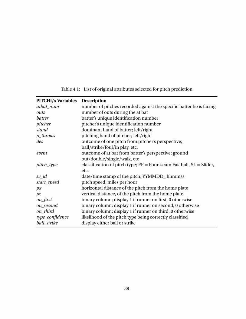
Table 4.1: List of original attributes selected for pitch prediction

PITCHf/x Variables Descriptionatbat_num number of pitches recorded against the specific batter he is facingouts number of outs during the at batbatter batter’s unique identification numberpitcher pitcher’s unique identification numberstand dominant hand of batter; left/rightp_throws pitching hand of pitcher; left/rightdes outcome of one pitch from pitcher’s perspective;

ball/strike/foul/in play, etc.event outcome of at bat from batter’s perspective; ground

out/double/single/walk, etcpitch_type classification of pitch type; FF = Four-seam Fastball, SL = Slider,

etc.sv_id date/time stamp of the pitch; YYMMDD_ hhmmssstart_speed pitch speed, miles per hourpx horizontal distance of the pitch from the home platepz vertical distance, of the pitch from the home plateon_first binary column; display 1 if runner on first, 0 otherwiseon_second binary column; display 1 if runner on second, 0 otherwiseon_third binary column; display 1 if runner on third, 0 otherwisetype_confidence likelihood of the pitch type being correctly classifiedball_strike display either ball or strike

39

with every pitch thrown in Major League Baseball (MLB) games. The system, which was

installed in every MLB stadium circa 2006, records useful information for every pitch.

Some measurements such as the initial velocity, plate velocity, release point, spin angle

and spin rate are useful to characterize the pitch type (e.g., fastball, curveball, changeup,

knuckleball). The pitch type is determined by PITCHf/x using a proprietary classification

algorithm. Because of the large number of MLB games in a season (2430) and the high

number of pitches thrown in a game (an average of 146 pitches per team), PITCHf/x provides

a rich data set on which to train and evaluate methodologies for pitch classification and

prediction. Pitch analysis can either be performed using the measurements provided by

PITCHf/x in their raw form or by using data derived features. Each of the recorded pitches

is classified by the PITCHf/x proprietary algorithm and provided with measurement data.

For the purposes of analysis, the proprietary PITCHf/x classification algorithm is assumed

to generally represent truth. For example, in [9] and [10], several classification algorithms

including Support Vector Machine (SVM) and Bayesian classifiers were used to classify pitch

types based on features derived from PITCHf/x data. The authors evaluated classification

algorithms both on accuracy, as compared to the truth classes provided by PITCHf/x,

and speed. In addition, Linear Discrimination Analysis (LDA) and Principal Component

Analysis (PCA) were used to evaluate feature dimension reduction useful for classification.

The pitch classification was evaluated using a set of pitchers’ data from the 2011 MLB

regular season.

Another important area of ongoing research is pitch prediction, which could have sig-

nificant real-world applications and potentially provides MLB managers with the statistical

competitive edge in simulation using in training and coaching. One example of research

on this topic is the work by [31], who use a Linear Support Vector Machine (SVM-L) to

perform binary (fastball vs. nonfastball) classification on pitches of unknown type. The

SVM-L model is trained on PITCHf/x data from pitches thrown in 2008 and tested on data

from 2009. Across all pitchers, an average prediction accuracy of roughly 70 percent is

obtained, though pitcher specific accuracies vary.

Other related pitch data analysis in the literature, such as [65], which examines the

pitching strategy of major league pitchers, specifically determining whether or not they

(from a game theoretic approach) implement optimally mixed strategies for handling

batters. The paper concludes that pitchers do mix optimally with respect to the pitch

40

variable and behave rationally relative to the result of any given pitch.

Our study provides a machine learning approach to pitch prediction, using a binary

classification method to predict pitch type, defined as fastball vs. nonfastball. A distinct

difference in our approach is the introduction of an adaptive strategy to feature selection

to mimic portions of pitchers’ behavior. This allows the machine learning algorithm to

select different sets of features in different situations to train the classifiers. The features

used contain not only original features, but also hybrid features that are created to better

resemble the way pitchers seem to process data. Additionally, cross validation is imple-

mented to detect and avoid overfitting in our predictions. Overall, the prediction accuracy

is improved by approximately 8% from results published in [31]. A report of our initial effort

in this study can be found in [32].

4.3 Our Model

4.3.1 Dynamic Feature Selection Approach

A key difference between our approach and former research of [31] is the feature selection

methodology. Rather than using a static set of features, an adaptive set is used for each

pitcher/count pair. This allows the algorithm to adapt to achieve the best prediction

performance result possible on each pitcher/count pair of data.

In baseball there are a number of factors that influence a pitcher’s decision, either

consciously or unconsciously. For example, one pitcher may not like to throw curveballs

during the daytime because the increased visibility makes them easier to spot; however,

another pitcher may not make his pitching decisions based on the time of the game. In

order to maximize accuracy of a prediction model, one must try to accommodate each of

these factors. For example, a pitcher may have particularly good control of a certain pitch

and thus favors that pitch, but how can one create a feature to represent its favorability? A

potential approach is to create a feature that measures the pitcher’s success with a pitch

since the beginning of the season, or the previous game, or even the previous batter faced.

Which features would best capture the true effect of his preference for that pitch? The

answer is that each of these approaches may be best in different situations, so they all

must be considered for best accuracy. Pitchers have different dominant pitches, strategies

41

and experiences; in order to maximize accuracy, our model must be adaptable to various

pitching situations. It is noted that in feature space, pitches of same pitch type from different

pitchers look different, so classifiers must be trained on each pitcher separately.

Of course, simply adding many features to our model is not necessarily favorable due

to the curse of dimensionality. In addition, some features might not be relevant to pitch

prediction. Our approach is to change the problem of predicting a pitch into predicting

a pitch for each pitcher in a given count. Count, which gives the number of balls and

strikes in an at-bat situation, has a significant effect on the pitcher/batter relationship.

For example, study by [35] showed that average slugging percentage (a weighted measure

of on-base frequency of a batter) is significantly lower in counts that favor the pitcher;

however, for neutral counts or counts that favor the batter, there is no significant difference

in average slugging percentage. In addition, [31] concluded that pitchers are much more

predictable when there are more balls than strikes. These studies show that count is an

important factor in making pitch predictions. In order to maximize accuracy, we take an

additional step by choosing a most relevant pool of features from the entire available set for

each pitcher/count pair. This allows us to maintain our adaptive strategy while controlling

dimensionality.

An example of this strategy is shown in Figure 4.1, where we present the selection of

predictive features from group 1 for the MLB pitcher Miguel Batista using the data from the

2008 and 2009 seasons when he played for the Seattle Mariners. This figure is segmented by

pitching scenarios including batter-favored count, neutral count, and pitcher-favored count.

Note that the batter-favored and pitcher-favored counts tend to result in dissimilar feature

sets being selected, whereas the neutral counts tend to result in a mixture thereof. More

specifically, feature number 6 (lifetime percentage of fastballs thrown) is highly indicative

of the status quo or standard pitching, it is selected for almost every count except the

batter-favored counts (i.e., 3-0, 3-1, 2-0,1-0), where it is selected only once out of 4 counts

(pitch count, 1-0). This shows that our feature selection model adapts to the game situation.

The pitcher behaves nominally until he is in an unfavorable count, when he often changes

his behavior and a priori value of fastball is no longer selected to use in prediction. We also

apply this analysis to the other 5 groups of features. It is noted that each count situation

yields a different set of features. There are certainly overlapping features, but there is no

unique set of features that are chosen in all counts.

42

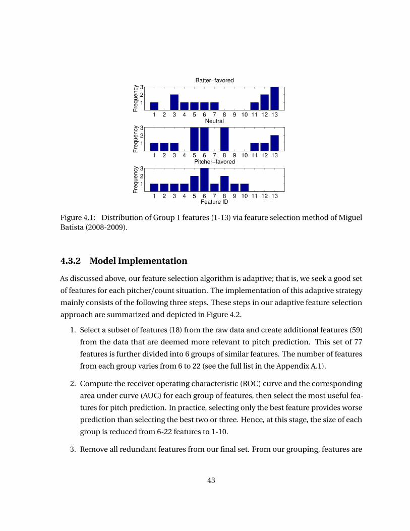
1 2 3 4 5 6 7 8 9 10 11 12 13

1

2

3Batter−favored

Fre

qu

en

cy

1 2 3 4 5 6 7 8 9 10 11 12 13

1

2

3Neutral

Fre

qu

en

cy

1 2 3 4 5 6 7 8 9 10 11 12 13

1

2

3Pitcher−favored

Feature ID

Fre

qu

en

cy

Figure 4.1: Distribution of Group 1 features (1-13) via feature selection method of MiguelBatista (2008-2009).

4.3.2 Model Implementation

As discussed above, our feature selection algorithm is adaptive; that is, we seek a good set

of features for each pitcher/count situation. The implementation of this adaptive strategy

mainly consists of the following three steps. These steps in our adaptive feature selection

approach are summarized and depicted in Figure 4.2.

1. Select a subset of features (18) from the raw data and create additional features (59)

from the data that are deemed more relevant to pitch prediction. This set of 77

features is further divided into 6 groups of similar features. The number of features

from each group varies from 6 to 22 (see the full list in the Appendix A.1).

2. Compute the receiver operating characteristic (ROC) curve and the corresponding

area under curve (AUC) for each group of features, then select the most useful fea-

tures for pitch prediction. In practice, selecting only the best feature provides worse

prediction than selecting the best two or three. Hence, at this stage, the size of each

group is reduced from 6-22 features to 1-10.

3. Remove all redundant features from our final set. From our grouping, features are

43

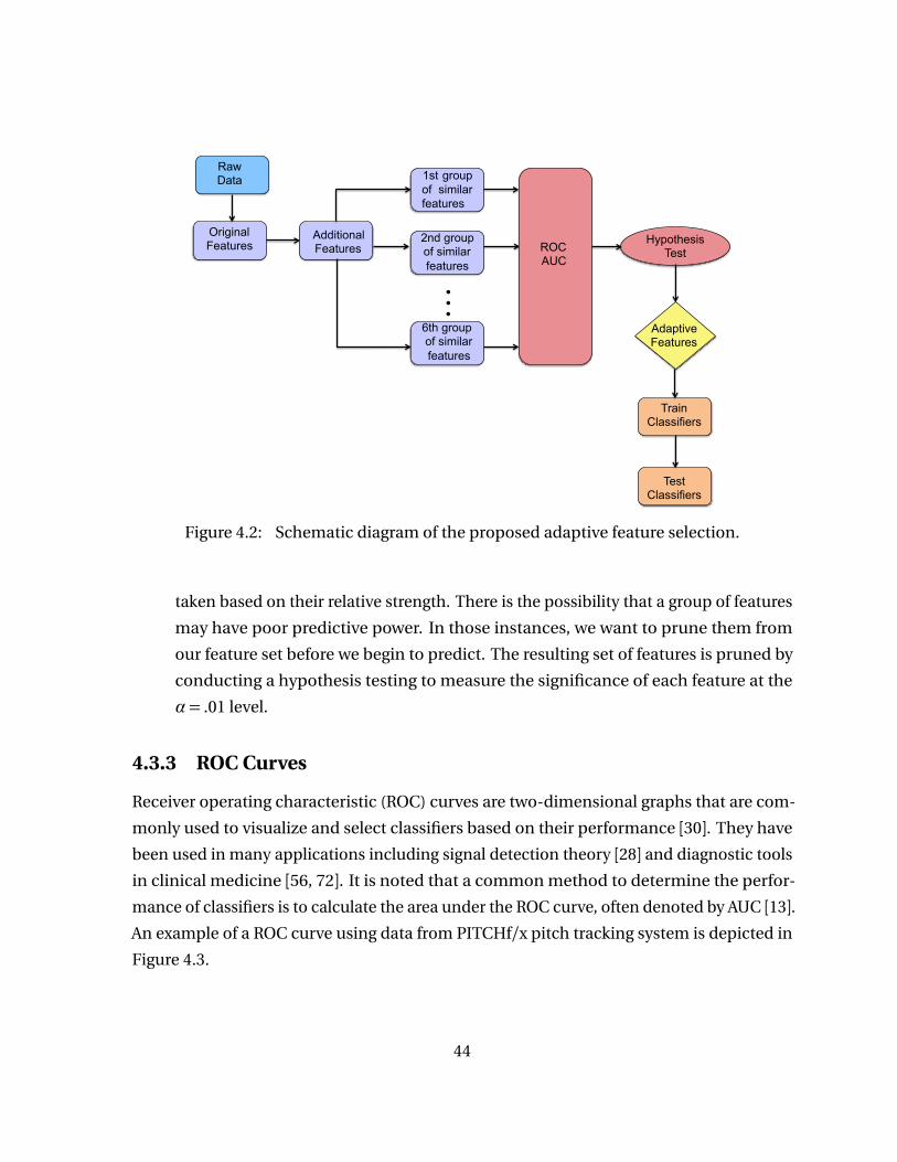
Raw Data

Original Features

1st group of similar features

Hypothesis Test

6th group of similar features

2nd group of similar features

Adaptive Features

Train Classifiers

Test Classifiers

Additional Features

⋮

ROC AUC

Figure 4.2: Schematic diagram of the proposed adaptive feature selection.

taken based on their relative strength. There is the possibility that a group of features

may have poor predictive power. In those instances, we want to prune them from

our feature set before we begin to predict. The resulting set of features is pruned by

conducting a hypothesis testing to measure the significance of each feature at the

α= .01 level.

4.3.3 ROC Curves

Receiver operating characteristic (ROC) curves are two-dimensional graphs that are com-

monly used to visualize and select classifiers based on their performance [30]. They have

been used in many applications including signal detection theory [28] and diagnostic tools

in clinical medicine [56, 72]. It is noted that a common method to determine the perfor-

mance of classifiers is to calculate the area under the ROC curve, often denoted by AUC [13].

An example of a ROC curve using data from PITCHf/x pitch tracking system is depicted in

Figure 4.3.

44

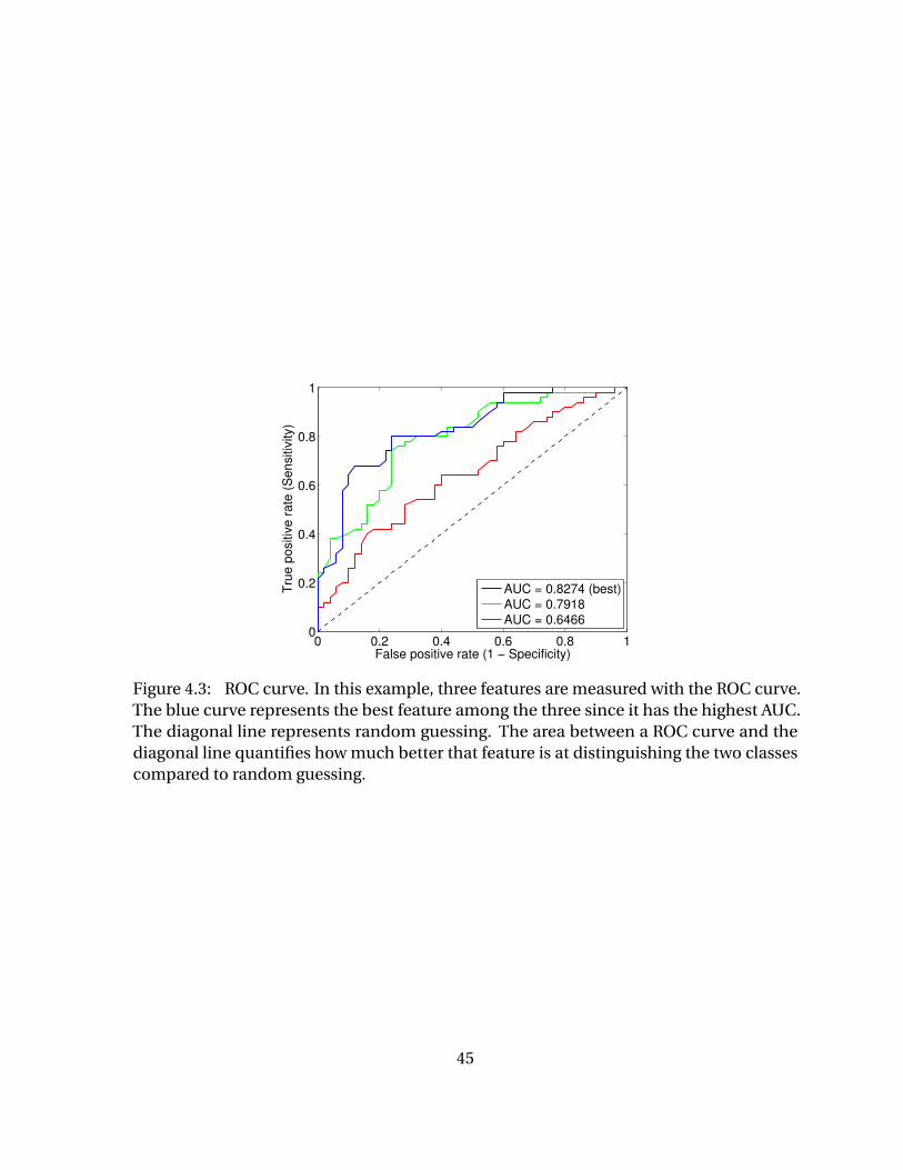
0 0.2 0.4 0.6 0.8 10

0.2

0.4

0.6

0.8

1

False positive rate (1 − Specificity)

Tru

e p

ositiv

e r

ate

(S

en

sitiv

ity)

AUC = 0.8274 (best)

AUC = 0.7918

AUC = 0.6466

Figure 4.3: ROC curve. In this example, three features are measured with the ROC curve.The blue curve represents the best feature among the three since it has the highest AUC.The diagonal line represents random guessing. The area between a ROC curve and thediagonal line quantifies how much better that feature is at distinguishing the two classescompared to random guessing.

45

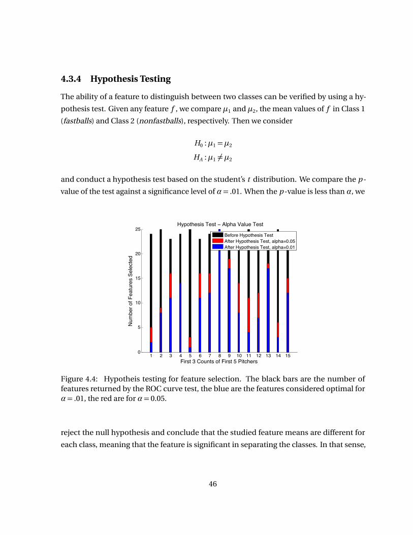
4.3.4 Hypothesis Testing

The ability of a feature to distinguish between two classes can be verified by using a hy-

pothesis test. Given any feature f , we compare µ1 and µ2, the mean values of f in Class 1

(fastballs) and Class 2 (nonfastballs), respectively. Then we consider

H0 :µ1 =µ2

HA :µ1 6=µ2

and conduct a hypothesis test based on the student’s t distribution. We compare the p -

value of the test against a significance level of α= .01. When the p -value is less than α, we

1 2 3 4 5 6 7 8 9 10 11 12 13 14 150

5

10

15

20

25Hypothesis Test − Alpha Value Test

First 3 Counts of First 5 Pitchers

Num

ber o

f Fea

ture

s Se

lect

ed

Before Hypothesis TestAfter Hypothesis Test, alpha=0.05After Hypothesis Test, alpha=0.01

Figure 4.4: Hypotheis testing for feature selection. The black bars are the number offeatures returned by the ROC curve test, the blue are the features considered optimal forα= .01, the red are for α= 0.05.

reject the null hypothesis and conclude that the studied feature means are different for

each class, meaning that the feature is significant in separating the classes. In that sense,

46

this test allows us to remove features which have insignificant separation power.

Figure 4.4 depicts the hypothesis testing step for the first 15 pitcher-count pairs in

our dataset. The number of features rise in the optimal set when we increase α = .01 to

α= .05 as expected. In our experiment, the accuracy, however, is lowered than the stricter

significant level. It is also important to notice that the number of the optimal features is

varying throughout different pitcher-count pairs.

4.3.5 Classification

Classification is the process of taking an unlabeled data observation and using some rule

or decision making process to assign a label to it as presented earlier in Chapter 2. Within

the scope of this study, classification represents determining the type of a pitch, i.e., given

a pitch x with characteristics xi , determine the pitch type x is. Several classification can be

used to accomplish this task. The methods used in this study are the k -nearest neighbor

(k -NN), the Linear Discriminant Analysis (LDA) and the Support Vector Machine (SVM),

see chapter 2 for a discussion of each method.

4.4 Results Analysis

To form a baseline for our prediction results, the prediction model is compared against the

naive guess model. The naive guess simply returns the most frequent pitch type thrown

by each pitcher, calculated from the training set, see [31]. The improvement factor I is

calculated as follows:

I =A1−A0

A0×100 (4.1)

where A0 and A1 denotes the accuracies of naive guess and our model, respectively.

4.4.1 Overall Results

We apply prediction techniques to all pitchers who threw at least 750 pitches in both 2008

and 2009. After performing feature selection on each data subset, each classifier (see

Appendix A.3) is trained on data from 2008 and tested on data from 2009. The average

classification accuracy for each classifier is computed for test points with a type confidence

47

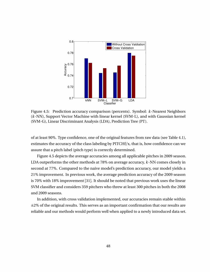
kNN SVM−L SVM−G LDA0.7

0.72

0.74

0.76

0.78

0.8

Classifier

Accu

racy

Without Cross Valdiation

Cross Validation

Figure 4.5: Prediction accuracy comparison (percents). Symbol: k -Nearest Neighbors(k -NN), Support Vector Machine with linear kernel (SVM-L), and with Gaussian kernel(SVM-G), Linear Discriminant Analysis (LDA), Prediction Tree (PT).

of at least 90%. Type confidence, one of the original features from raw data (see Table 4.1),

estimates the accuracy of the class labeling by PITCHf/x, that is, how confidence can we

assure that a pitch label (pitch type) is correctly determined.

Figure 4.5 depicts the average accuracies among all applicable pitches in 2009 season.

LDA outperforms the other methods at 78% on average accuracy, k -NN comes closely in

second at 77%. Compared to the naive model’s prediction accuracy, our model yields a

21% improvement. In previous work, the average prediction accuracy of the 2009 season

is 70% with 18% improvement [31]. It should be noted that previous work uses the linear

SVM classifier and considers 359 pitchers who threw at least 300 pitches in both the 2008

and 2009 seasons.

In addition, with cross validation implemented, our accuracies remain stable within

±2% of the original results. This serves as an important confirmation that our results are

reliable and our methods would perform well when applied to a newly introduced data set.

48

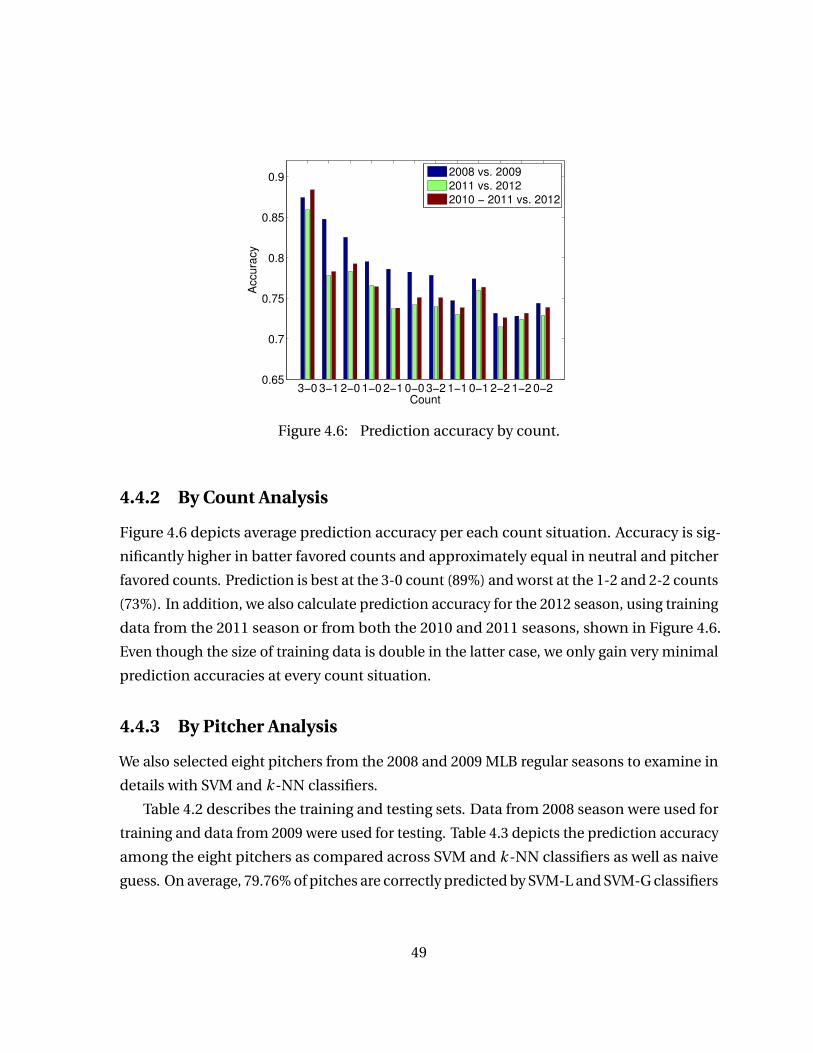
3−0 3−1 2−0 1−0 2−1 0−0 3−2 1−1 0−1 2−2 1−2 0−20.65

0.7

0.75

0.8

0.85

0.9

Count

Accu

racy

2008 vs. 2009

2011 vs. 2012

2010 − 2011 vs. 2012

Figure 4.6: Prediction accuracy by count.

4.4.2 By Count Analysis

Figure 4.6 depicts average prediction accuracy per each count situation. Accuracy is sig-

nificantly higher in batter favored counts and approximately equal in neutral and pitcher

favored counts. Prediction is best at the 3-0 count (89%) and worst at the 1-2 and 2-2 counts

(73%). In addition, we also calculate prediction accuracy for the 2012 season, using training

data from the 2011 season or from both the 2010 and 2011 seasons, shown in Figure 4.6.

Even though the size of training data is double in the latter case, we only gain very minimal

prediction accuracies at every count situation.

4.4.3 By Pitcher Analysis

We also selected eight pitchers from the 2008 and 2009 MLB regular seasons to examine in

details with SVM and k -NN classifiers.

Table 4.2 describes the training and testing sets. Data from 2008 season were used for

training and data from 2009 were used for testing. Table 4.3 depicts the prediction accuracy

among the eight pitchers as compared across SVM and k -NN classifiers as well as naive

guess. On average, 79.76% of pitches are correctly predicted by SVM-L and SVM-G classifiers

49

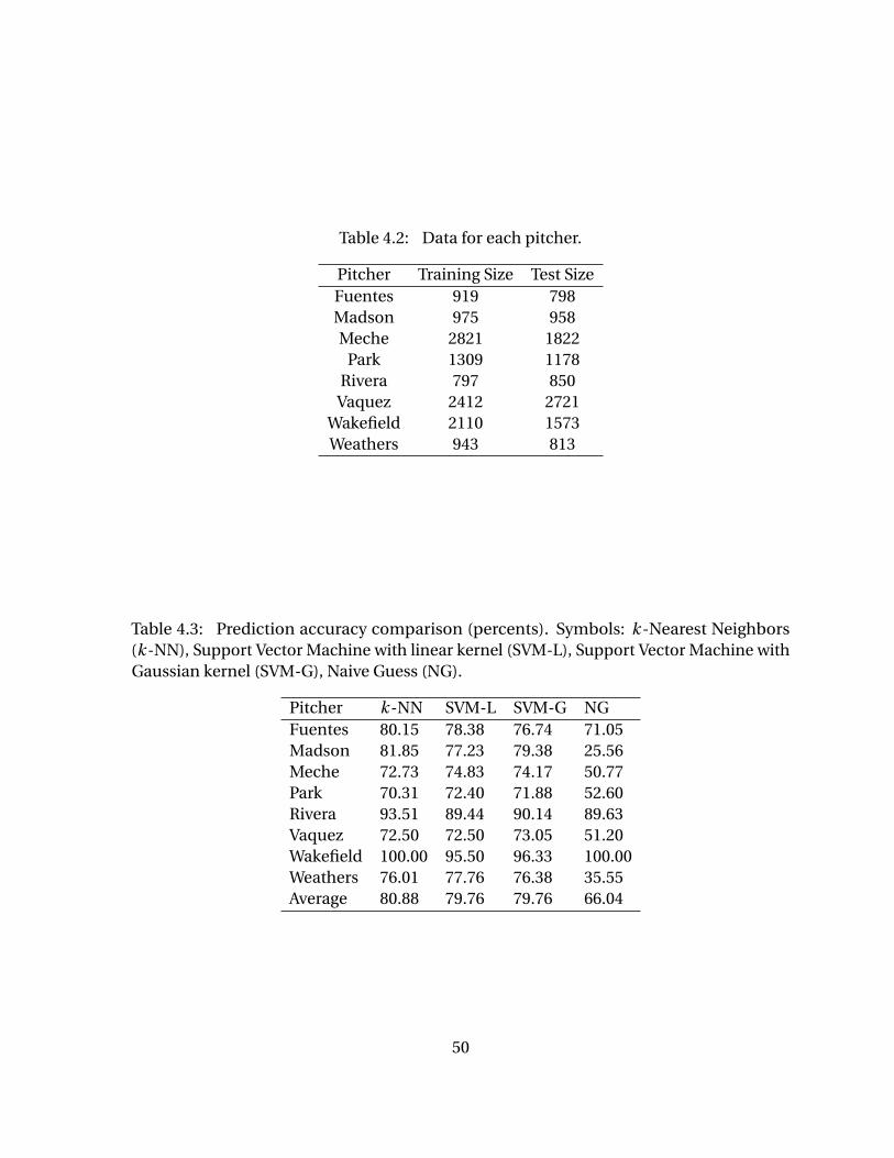
Table 4.2: Data for each pitcher.

Pitcher Training Size Test SizeFuentes 919 798Madson 975 958Meche 2821 1822

Park 1309 1178Rivera 797 850Vaquez 2412 2721

Wakefield 2110 1573Weathers 943 813

Table 4.3: Prediction accuracy comparison (percents). Symbols: k -Nearest Neighbors(k -NN), Support Vector Machine with linear kernel (SVM-L), Support Vector Machine withGaussian kernel (SVM-G), Naive Guess (NG).

Pitcher k -NN SVM-L SVM-G NGFuentes 80.15 78.38 76.74 71.05Madson 81.85 77.23 79.38 25.56Meche 72.73 74.83 74.17 50.77Park 70.31 72.40 71.88 52.60Rivera 93.51 89.44 90.14 89.63Vaquez 72.50 72.50 73.05 51.20Wakefield 100.00 95.50 96.33 100.00Weathers 76.01 77.76 76.38 35.55Average 80.88 79.76 79.76 66.04

50

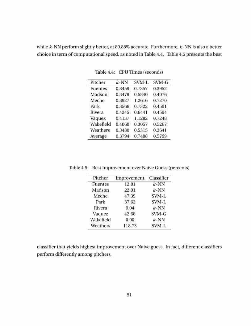
while k -NN perform slightly better, at 80.88% accurate. Furthermore, k -NN is also a better

choice in term of computational speed, as noted in Table 4.4. Table 4.5 presents the best

Table 4.4: CPU Times (seconds)

Pitcher k -NN SVM-L SVM-GFuentes 0.3459 0.7357 0.3952Madson 0.3479 0.5840 0.4076Meche 0.3927 1.2616 0.7270Park 0.3566 0.7322 0.4591Rivera 0.4245 0.6441 0.4594Vaquez 0.4137 1.1282 0.7248Wakefield 0.4060 0.3057 0.5267Weathers 0.3480 0.5315 0.3641Average 0.3794 0.7408 0.5799

Table 4.5: Best Improvement over Naive Guess (percents)

Pitcher Improvement ClassifierFuentes 12.81 k -NNMadson 22.01 k -NNMeche 47.39 SVM-L

Park 37.62 SVM-LRivera 0.04 k -NNVaquez 42.68 SVM-G

Wakefield 0.00 k -NNWeathers 118.73 SVM-L

classifier that yields highest improvement over Naive guess. In fact, different classifiers

perform differently among pitchers.

51

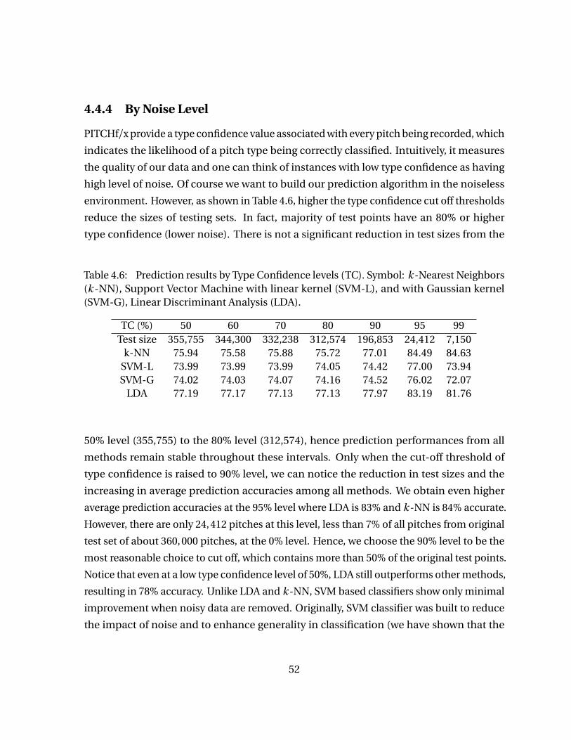
4.4.4 By Noise Level

PITCHf/x provide a type confidence value associated with every pitch being recorded, which

indicates the likelihood of a pitch type being correctly classified. Intuitively, it measures

the quality of our data and one can think of instances with low type confidence as having

high level of noise. Of course we want to build our prediction algorithm in the noiseless

environment. However, as shown in Table 4.6, higher the type confidence cut off thresholds

reduce the sizes of testing sets. In fact, majority of test points have an 80% or higher

type confidence (lower noise). There is not a significant reduction in test sizes from the

Table 4.6: Prediction results by Type Confidence levels (TC). Symbol: k -Nearest Neighbors(k -NN), Support Vector Machine with linear kernel (SVM-L), and with Gaussian kernel(SVM-G), Linear Discriminant Analysis (LDA).

TC (%) 50 60 70 80 90 95 99Test size 355,755 344,300 332,238 312,574 196,853 24,412 7,150

k-NN 75.94 75.58 75.88 75.72 77.01 84.49 84.63SVM-L 73.99 73.99 73.99 74.05 74.42 77.00 73.94SVM-G 74.02 74.03 74.07 74.16 74.52 76.02 72.07

LDA 77.19 77.17 77.13 77.13 77.97 83.19 81.76

50% level (355,755) to the 80% level (312,574), hence prediction performances from all

methods remain stable throughout these intervals. Only when the cut-off threshold of

type confidence is raised to 90% level, we can notice the reduction in test sizes and the

increasing in average prediction accuracies among all methods. We obtain even higher

average prediction accuracies at the 95% level where LDA is 83% and k -NN is 84% accurate.

However, there are only 24, 412 pitches at this level, less than 7% of all pitches from original

test set of about 360, 000 pitches, at the 0% level. Hence, we choose the 90% level to be the

most reasonable choice to cut off, which contains more than 50% of the original test points.

Notice that even at a low type confidence level of 50%, LDA still outperforms other methods,

resulting in 78% accuracy. Unlike LDA and k -NN, SVM based classifiers show only minimal

improvement when noisy data are removed. Originally, SVM classifier was built to reduce

the impact of noise and to enhance generality in classification (we have shown that the

52

SVM has Tikhonov regularization embedded in section 3.1 ). Furthermore, only the support

vectors (a subset of training data) are used in the final decision function while the rest of the

training data are not considered (section 2.3). It would be very likely that those data points

with low level of type confidence are not selected to be support vectors. Thus, SVM results

are consistency among different levels of type confidence threshold cut-off. This is indeed

the motivation for us to focus on implement SVM based classifier for our medical diagnosis

work where the datasets are much smaller and the presence of noise is not negligible.

53

CHAPTER

5

MEDICAL DIAGNOSIS

Medical diagnostic decision support systems (MDSS) play important role in assisting physi-

cians with making clinical decisions. Berner et al. (1999) suggest that physicians’ perfor-

mance can be strongly influenced by the quality of the information the system 1 produce

and the type of cases on which the system is used. Physicians’ diagnostic performance is

significant higher on easier cases for which MDSS could provide higher-quality information

[46]. The less than ideal performance on harder cases motivates researchers to seek for

better diagnostic models because the cost of false negative 2 is often too high in health care.

1In this research, a national sample of 67 internists, 35 family physicians, and 6 other physicians use QuickMedical Reference diagnostic support system to assist them in the diagnosis of clinical case. Three sets ofeight cases, stratified by diagnostic difficulty and the potential of QMR to produce high-quality information,were used. The effects of using QMR on three measures of physicians diagnostic performance were analyzedusing analyses of variance [46].

2False negative refers to incorrectly indicating a person does not have a disease or condition when theperson actually does have it.

54

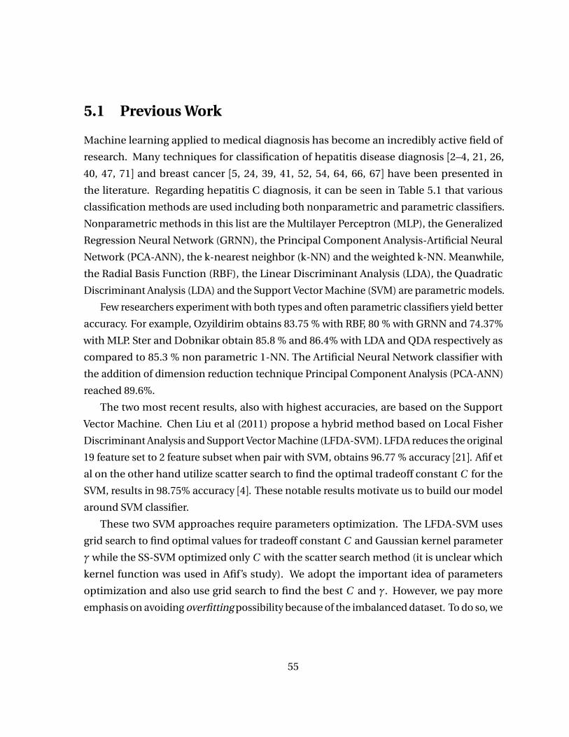
5.1 Previous Work

Machine learning applied to medical diagnosis has become an incredibly active field of

research. Many techniques for classification of hepatitis disease diagnosis [2–4, 21, 26,

40, 47, 71] and breast cancer [5, 24, 39, 41, 52, 54, 64, 66, 67] have been presented in

the literature. Regarding hepatitis C diagnosis, it can be seen in Table 5.1 that various

classification methods are used including both nonparametric and parametric classifiers.

Nonparametric methods in this list are the Multilayer Perceptron (MLP), the Generalized

Regression Neural Network (GRNN), the Principal Component Analysis-Artificial Neural

Network (PCA-ANN), the k-nearest neighbor (k-NN) and the weighted k-NN. Meanwhile,

the Radial Basis Function (RBF), the Linear Discriminant Analysis (LDA), the Quadratic

Discriminant Analysis (LDA) and the Support Vector Machine (SVM) are parametric models.

Few researchers experiment with both types and often parametric classifiers yield better

accuracy. For example, Ozyildirim obtains 83.75 % with RBF, 80 % with GRNN and 74.37%

with MLP. Ster and Dobnikar obtain 85.8 % and 86.4% with LDA and QDA respectively as

compared to 85.3 % non parametric 1-NN. The Artificial Neural Network classifier with

the addition of dimension reduction technique Principal Component Analysis (PCA-ANN)

reached 89.6%.

The two most recent results, also with highest accuracies, are based on the Support

Vector Machine. Chen Liu et al (2011) propose a hybrid method based on Local Fisher

Discriminant Analysis and Support Vector Machine (LFDA-SVM). LFDA reduces the original

19 feature set to 2 feature subset when pair with SVM, obtains 96.77 % accuracy [21]. Afif et

al on the other hand utilize scatter search to find the optimal tradeoff constant C for the

SVM, results in 98.75% accuracy [4]. These notable results motivate us to build our model

around SVM classifier.

These two SVM approaches require parameters optimization. The LFDA-SVM uses

grid search to find optimal values for tradeoff constant C and Gaussian kernel parameter

γwhile the SS-SVM optimized only C with the scatter search method (it is unclear which

kernel function was used in Afif’s study). We adopt the important idea of parameters

optimization and also use grid search to find the best C and γ. However, we pay more

emphasis on avoiding overfitting possibility because of the imbalanced dataset. To do so, we

55

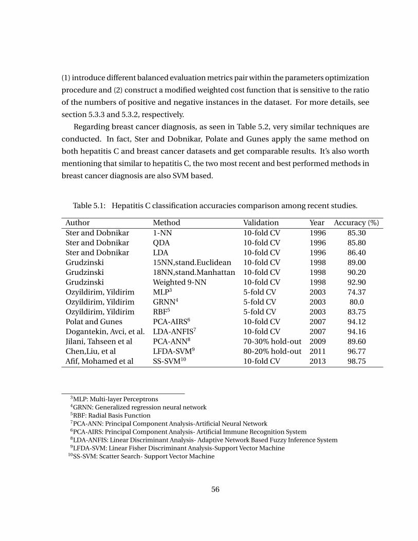
(1) introduce different balanced evaluation metrics pair within the parameters optimization

procedure and (2) construct a modified weighted cost function that is sensitive to the ratio

of the numbers of positive and negative instances in the dataset. For more details, see

section 5.3.3 and 5.3.2, respectively.

Regarding breast cancer diagnosis, as seen in Table 5.2, very similar techniques are

conducted. In fact, Ster and Dobnikar, Polate and Gunes apply the same method on

both hepatitis C and breast cancer datasets and get comparable results. It’s also worth

mentioning that similar to hepatitis C, the two most recent and best performed methods in

breast cancer diagnosis are also SVM based.

Table 5.1: Hepatitis C classification accuracies comparison among recent studies.

Author Method Validation Year Accuracy (%)Ster and Dobnikar 1-NN 10-fold CV 1996 85.30Ster and Dobnikar QDA 10-fold CV 1996 85.80Ster and Dobnikar LDA 10-fold CV 1996 86.40Grudzinski 15NN,stand.Euclidean 10-fold CV 1998 89.00Grudzinski 18NN,stand.Manhattan 10-fold CV 1998 90.20Grudzinski Weighted 9-NN 10-fold CV 1998 92.90Ozyildirim, Yildirim MLP3 5-fold CV 2003 74.37Ozyildirim, Yildirim GRNN4 5-fold CV 2003 80.0Ozyildirim, Yildirim RBF5 5-fold CV 2003 83.75Polat and Gunes PCA-AIRS6 10-fold CV 2007 94.12Dogantekin, Avci, et al. LDA-ANFIS7 10-fold CV 2007 94.16Jilani, Tahseen et al PCA-ANN8 70-30% hold-out 2009 89.60Chen,Liu, et al LFDA-SVM9 80-20% hold-out 2011 96.77Afif, Mohamed et al SS-SVM10 10-fold CV 2013 98.75

3MLP: Multi-layer Perceptrons4GRNN: Generalized regression neural network5RBF: Radial Basis Function7PCA-ANN: Principal Component Analysis-Artificial Neural Network6PCA-AIRS: Principal Component Analysis- Artificial Immune Recognition System8LDA-ANFIS: Linear Discriminant Analysis- Adaptive Network Based Fuzzy Inference System9LFDA-SVM: Linear Fisher Discriminant Analysis-Support Vector Machine

10SS-SVM: Scatter Search- Support Vector Machine

56

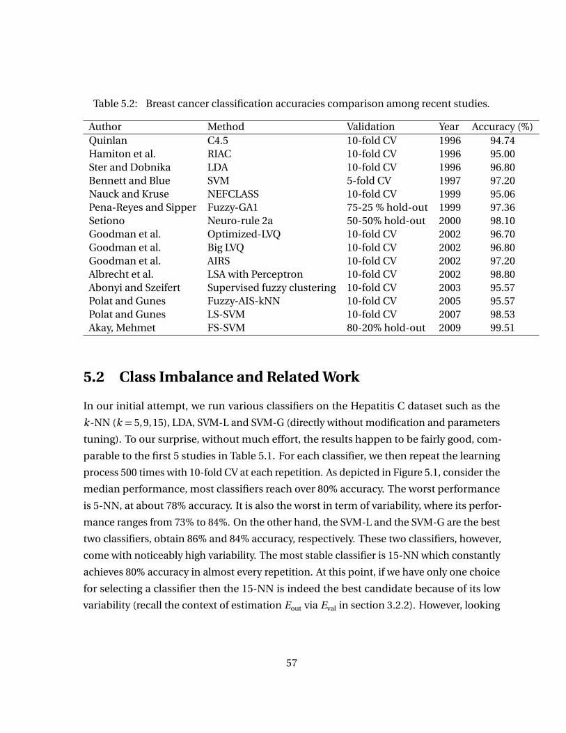
Table 5.2: Breast cancer classification accuracies comparison among recent studies.

Author Method Validation Year Accuracy (%)Quinlan C4.5 10-fold CV 1996 94.74Hamiton et al. RIAC 10-fold CV 1996 95.00Ster and Dobnika LDA 10-fold CV 1996 96.80Bennett and Blue SVM 5-fold CV 1997 97.20Nauck and Kruse NEFCLASS 10-fold CV 1999 95.06Pena-Reyes and Sipper Fuzzy-GA1 75-25 % hold-out 1999 97.36Setiono Neuro-rule 2a 50-50% hold-out 2000 98.10Goodman et al. Optimized-LVQ 10-fold CV 2002 96.70Goodman et al. Big LVQ 10-fold CV 2002 96.80Goodman et al. AIRS 10-fold CV 2002 97.20Albrecht et al. LSA with Perceptron 10-fold CV 2002 98.80Abonyi and Szeifert Supervised fuzzy clustering 10-fold CV 2003 95.57Polat and Gunes Fuzzy-AIS-kNN 10-fold CV 2005 95.57Polat and Gunes LS-SVM 10-fold CV 2007 98.53Akay, Mehmet FS-SVM 80-20% hold-out 2009 99.51

5.2 Class Imbalance and Related Work

In our initial attempt, we run various classifiers on the Hepatitis C dataset such as the

k -NN (k = 5, 9, 15), LDA, SVM-L and SVM-G (directly without modification and parameters

tuning). To our surprise, without much effort, the results happen to be fairly good, com-

parable to the first 5 studies in Table 5.1. For each classifier, we then repeat the learning

process 500 times with 10-fold CV at each repetition. As depicted in Figure 5.1, consider the

median performance, most classifiers reach over 80% accuracy. The worst performance

is 5-NN, at about 78% accuracy. It is also the worst in term of variability, where its perfor-

mance ranges from 73% to 84%. On the other hand, the SVM-L and the SVM-G are the best

two classifiers, obtain 86% and 84% accuracy, respectively. These two classifiers, however,

come with noticeably high variability. The most stable classifier is 15-NN which constantly

achieves 80% accuracy in almost every repetition. At this point, if we have only one choice

for selecting a classifier then the 15-NN is indeed the best candidate because of its low

variability (recall the context of estimation Eout via Eval in section 3.2.2). However, looking

57

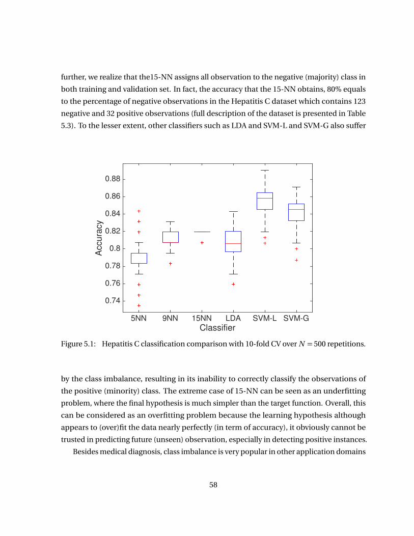
further, we realize that the15-NN assigns all observation to the negative (majority) class in

both training and validation set. In fact, the accuracy that the 15-NN obtains, 80% equals

to the percentage of negative observations in the Hepatitis C dataset which contains 123

negative and 32 positive observations (full description of the dataset is presented in Table

5.3). To the lesser extent, other classifiers such as LDA and SVM-L and SVM-G also suffer

Classifier5NN 9NN 15NN LDA SVM-L SVM-G

Accu

racy

0.74

0.76

0.78

0.8

0.82

0.84

0.86

0.88

Figure 5.1: Hepatitis C classification comparison with 10-fold CV over N = 500 repetitions.

by the class imbalance, resulting in its inability to correctly classify the observations of

the positive (minority) class. The extreme case of 15-NN can be seen as an underfitting

problem, where the final hypothesis is much simpler than the target function. Overall, this

can be considered as an overfitting problem because the learning hypothesis although

appears to (over)fit the data nearly perfectly (in term of accuracy), it obviously cannot be

trusted in predicting future (unseen) observation, especially in detecting positive instances.

Besides medical diagnosis, class imbalance is very popular in other application domains

58

such as gene profiling, (email) spam detection and credit card fraud detection. For example,

an imbalance of 100 to 1 exists in fraud detection [53]. Classifiers perform poorly on

unbalanced datasets because they are often designed to output the simplest hypothesis

that best fits the data. For example, recall the soft-margin SVM (section 2.3.2) which can be

seen as an Tikhonov regularization (section 3.1) to reduce model complexity. This approach

works well on balanced dataset (pitch prediction in previous chapter) but it often fails with

highly unbalanced datasets where the simplest model is often the one that classifies every

instance as negative. Thus, the classifiers consider positive instances as noise and ignore

them in the learning process.

Previous work on class imbalance classification can be categorized into two main divi-

sions: the data processing approach and the algorithmic approach [7, 34, 69].The data pro-

cessing approach is to adjust the class distribution of the data set by either under-sampling

the majority class or over-sampling the minority class. An example of under-sampling, pre-

sented in [42, 43], is to remove noisy and redundant majority instances. This method can be

challenging to use for small datasets (such as our Hepatitis C) where removing data points

can be expensive. Over-sampling is the opposite of under-sampling approach. Authors in

[20] suggest duplicating and/or interpolating minority instances under the method called

SMOTE 11. SMOTE assumes the neighborhood of a positive instance to be positive and

instances that locate between two positive instances are also positive. These assumptions

may not be true and can be data-dependent so again with small datasets, it would raise the

problem of inconsistency. For example, with cross validation, at each iteration, a different

partition of training and validation sets is formed, hence the idea of positive neighborhood

or the space between two positive instances may fail to remain intact. Furthermore, both

under-sampling and over-sampling techniques attempt to change the class distribution, in

turn, change class prior. Hence, it violates the assumption of many Bayesian classifiers,

such as LDA classifier where the discriminant function uses the estimate of the prior prob-

ability that a random chosen observation is associated with a certain class (section 2.2) [70].

Although the SVM is not directly affected by adjusting class prior, the inconsistency perfor-

mance with small datasets is enough for us to skip the under-sampling and over-sampling

techniques in our model.

11SMOTE: Synthetic Minority Oversampling Technique

59

The algorithmic approach, which is adopted in our study, is to bias the classifiers so

that they pay more attention to the positive instances. In the SVM regime, this is equivalent

to assign higher cost in misclassifying positive instances (we will discuss this further in

section 5.3.2). This idea is first suggested by Veropoulos et al [61] and its later extensions

can be found in [15, 45, 63]. Algorithmic approach also applies to other classifiers such as

[49] on modified multilayer perceptron or [25, 29] decision tree generator.

5.3 Model Implementation

Our benchmark is the study of Akbani et al [7]. The authors apply SVM with Veropoulos’s cost

sensitive approach [61] and implement SMOTE [20] in attempt to combat class imbalance.

Their model is tested with 10-fold cross validation on many unbalanced data sets, including

the UCI Hepatitis C dataset we use here. For our study, we employ the cost sensitive

approach (of using different penalty constants for different classes) combing with Gaussian

kernel parameter optimization on soft margin SVM. The steps of our diagnosis model is

depicted in Figure 5.2. Our model is implemented in the LIBSVM package for MATLAB.

LIBSVM software and its documentation can be found in [19].

5.3.1 Data Preprocessing

We perform our experiments on the Hepatitis C dataset taken from the UCI machine learn-

ing repository [44]. The dataset contains 155 observations, of which 32 of them are labeled

die while the remaining 123 observations are labeled live. Beside class label, 19 features are

associated with each observation from which 13 are binary values and 6 contains discrete

values. The description of all features in this dataset is presented in Table 5.3.

The data preparation process prior applying the SVM involves transforming categorical

feature to vector and scaling. The SVM requires that each instance is represented as a vector

of real numbers. To do this, we adapt the converting procedure suggested in [36], a vector

of length m is used to represent an m-category attribute. Only one of the m numbers is

one, and the others are zero. For example, a three-category attribute red, green, bluewill

be represented as (0,0,1), (0,1,0), and (1,0,0) instead of using a single indicator number

such as 1,2, and 3 [36].

60

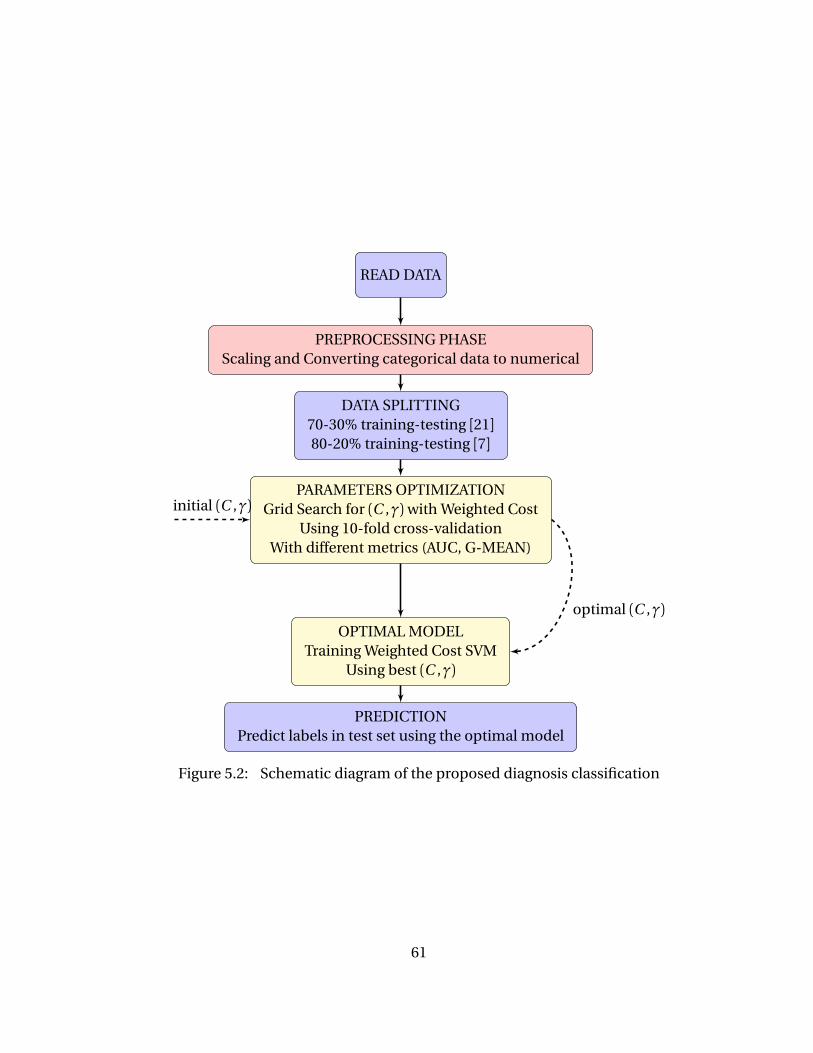
READ DATA

PREPROCESSING PHASEScaling and Converting categorical data to numerical

DATA SPLITTING70-30% training-testing [21]80-20% training-testing [7]

PARAMETERS OPTIMIZATIONGrid Search for (C ,γ)with Weighted Cost

Using 10-fold cross-validationWith different metrics (AUC, G-MEAN)

OPTIMAL MODELTraining Weighted Cost SVM

Using best (C ,γ)

PREDICTIONPredict labels in test set using the optimal model

initial (C ,γ)

optimal (C ,γ)

Figure 5.2: Schematic diagram of the proposed diagnosis classification

61

Table 5.3: Hepatitis C data: description of attributes. See Appendix B.1 for the definitionsof some of the attributes.

No Variable Values # of Missings1 Class Die (32), Alive (123) 02 AGE 7-78 03 SEX Male, Female 04 STEROID Yes, No 15 ANTIVIRALS Yes, No 06 FATIGUE Yes, No 17 MALAISE Yes, No 18 ANOREXIA Yes, No 19 LIVER BIG Yes, No 1010 LIVER FIRM Yes, No 1111 SPLEEN PALPABLE Yes, No 512 SPIDERS Yes, No 513 ASCITES Yes, No 514 VARICES Yes, No 515 BILIRUBIN 0.39- 4.0 616 ALK PHOSPHATE 33-250 2917 SGOT 13-500 418 ALBUMIN 2.1-6.0 1619 PROTIME 10-90 6720 HISTOLOGY Yes, No 20

62

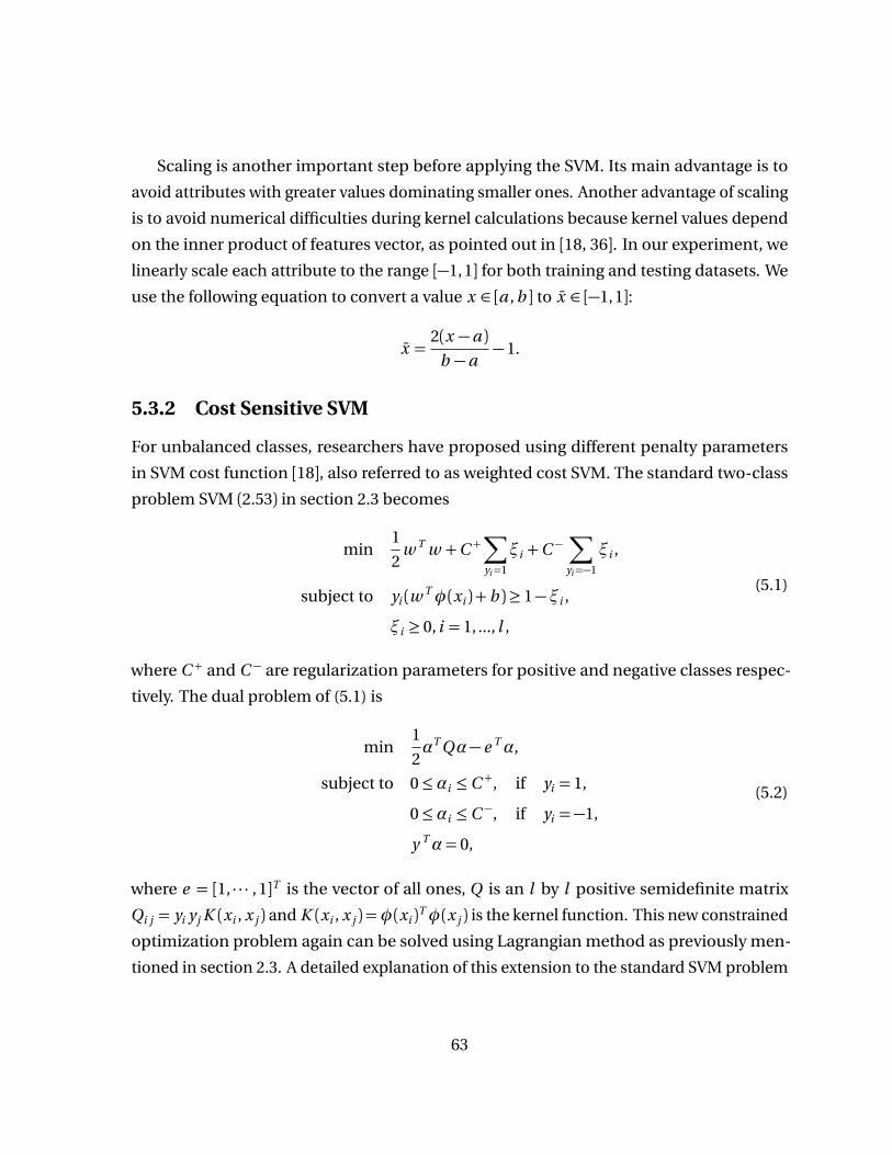
Scaling is another important step before applying the SVM. Its main advantage is to

avoid attributes with greater values dominating smaller ones. Another advantage of scaling

is to avoid numerical difficulties during kernel calculations because kernel values depend

on the inner product of features vector, as pointed out in [18, 36]. In our experiment, we

linearly scale each attribute to the range [−1,1] for both training and testing datasets. We

use the following equation to convert a value x ∈ [a , b ] to x ∈ [−1, 1]:

x =2(x −a )

b −a−1.

5.3.2 Cost Sensitive SVM

For unbalanced classes, researchers have proposed using different penalty parameters

in SVM cost function [18], also referred to as weighted cost SVM. The standard two-class

problem SVM (2.53) in section 2.3 becomes

min1

2w T w +C +

∑

yi=1

ξi +C −∑

yi=−1

ξi ,

subject to yi (wTφ(xi ) + b )≥ 1−ξi ,

ξi ≥ 0, i = 1, ..., l ,

(5.1)

where C + and C − are regularization parameters for positive and negative classes respec-

tively. The dual problem of (5.1) is

min1

2αT Qα− e Tα,

subject to 0≤αi ≤C +, if yi = 1,

0≤αi ≤C −, if yi =−1,

y Tα= 0,

(5.2)

where e = [1, · · · ,1]T is the vector of all ones, Q is an l by l positive semidefinite matrix

Qi j = yi yj K (xi , x j ) and K (xi , x j ) =φ(xi )Tφ(x j ) is the kernel function. This new constrained

optimization problem again can be solved using Lagrangian method as previously men-

tioned in section 2.3. A detailed explanation of this extension to the standard SVM problem

63

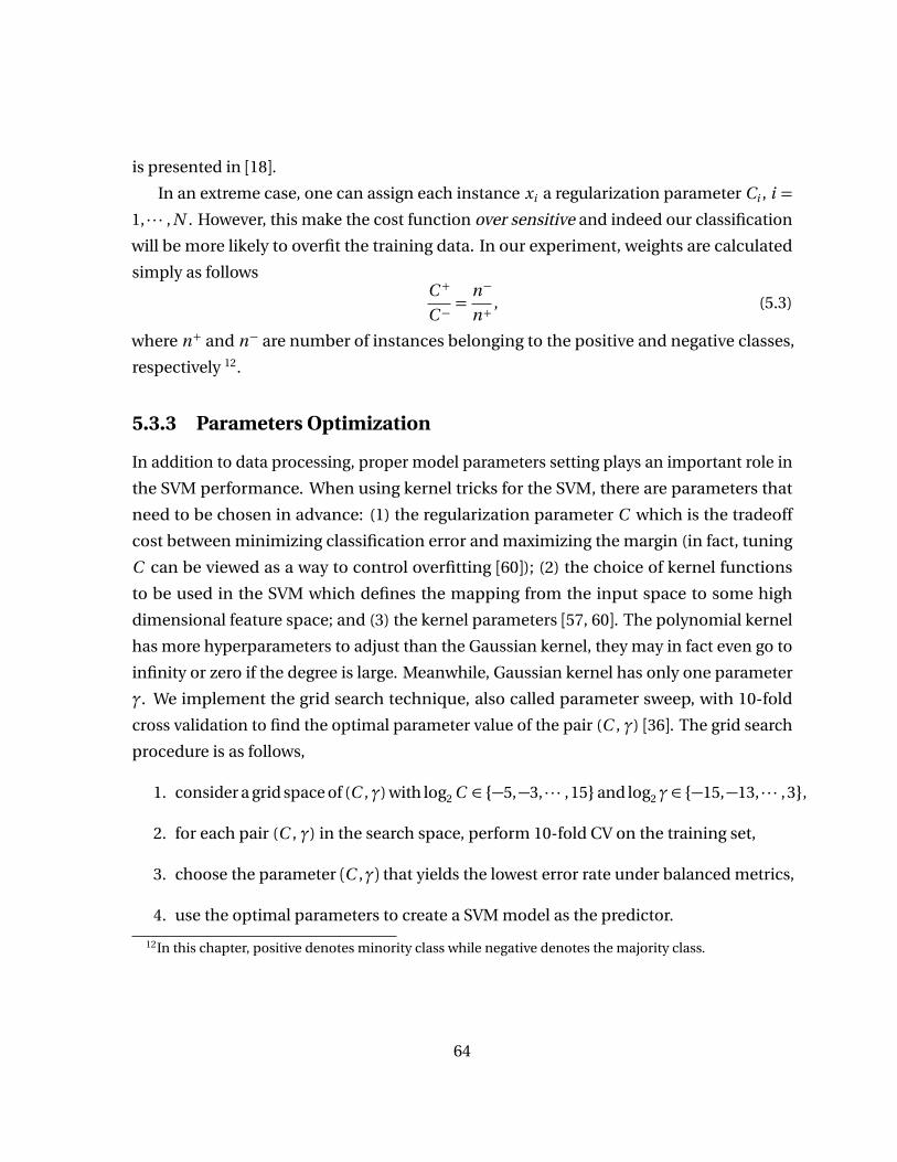
is presented in [18].

In an extreme case, one can assign each instance xi a regularization parameter Ci , i =

1, · · · , N . However, this make the cost function over sensitive and indeed our classification

will be more likely to overfit the training data. In our experiment, weights are calculated

simply as followsC +

C −=

n−

n+, (5.3)

where n+ and n− are number of instances belonging to the positive and negative classes,

respectively 12.

5.3.3 Parameters Optimization

In addition to data processing, proper model parameters setting plays an important role in

the SVM performance. When using kernel tricks for the SVM, there are parameters that

need to be chosen in advance: (1) the regularization parameter C which is the tradeoff

cost between minimizing classification error and maximizing the margin (in fact, tuning

C can be viewed as a way to control overfitting [60]); (2) the choice of kernel functions

to be used in the SVM which defines the mapping from the input space to some high

dimensional feature space; and (3) the kernel parameters [57, 60]. The polynomial kernel

has more hyperparameters to adjust than the Gaussian kernel, they may in fact even go to

infinity or zero if the degree is large. Meanwhile, Gaussian kernel has only one parameter

γ. We implement the grid search technique, also called parameter sweep, with 10-fold

cross validation to find the optimal parameter value of the pair (C , γ) [36]. The grid search

procedure is as follows,

1. consider a grid space of (C ,γ) with log2 C ∈ −5,−3, · · · , 15and log2γ ∈ −15,−13, · · · , 3,

2. for each pair (C , γ) in the search space, perform 10-fold CV on the training set,

3. choose the parameter (C ,γ) that yields the lowest error rate under balanced metrics,

4. use the optimal parameters to create a SVM model as the predictor.

12In this chapter, positive denotes minority class while negative denotes the majority class.

64

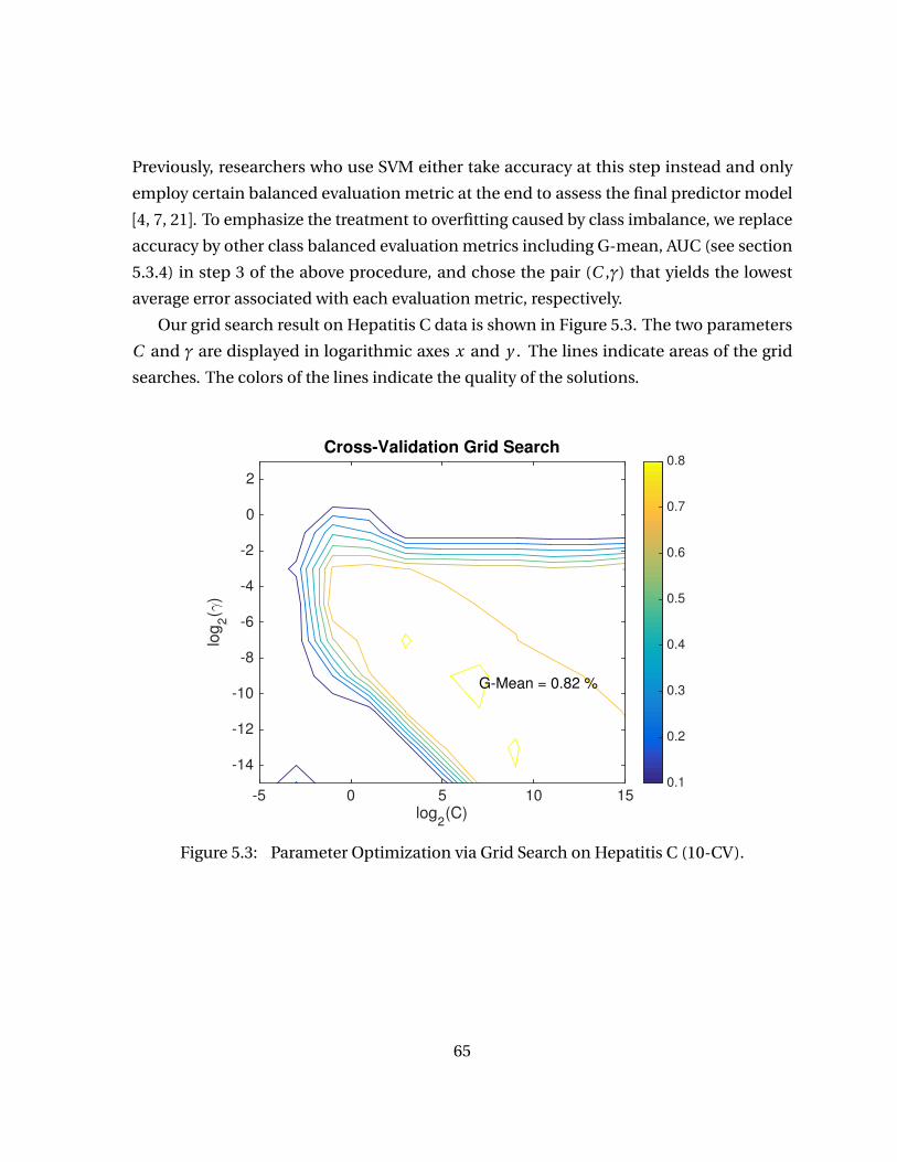
Previously, researchers who use SVM either take accuracy at this step instead and only

employ certain balanced evaluation metric at the end to assess the final predictor model

[4, 7, 21]. To emphasize the treatment to overfitting caused by class imbalance, we replace

accuracy by other class balanced evaluation metrics including G-mean, AUC (see section

5.3.4) in step 3 of the above procedure, and chose the pair (C ,γ) that yields the lowest

average error associated with each evaluation metric, respectively.

Our grid search result on Hepatitis C data is shown in Figure 5.3. The two parameters

C and γ are displayed in logarithmic axes x and y . The lines indicate areas of the grid

searches. The colors of the lines indicate the quality of the solutions.

G-Mean = 0.82 %

Cross-Validation Grid Search

log2(C)

-5 0 5 10 15

log

2(γ

)

-14

-12

-10

-8

-6

-4

-2

0

2

0.1

0.2

0.3

0.4

0.5

0.6

0.7

0.8

Figure 5.3: Parameter Optimization via Grid Search on Hepatitis C (10-CV).

65

5.3.4 Evaluation Metrics

Accuracy is a poor choice for model evaluation on unbalanced datasets as seen in previously.

The machine learning and medical communities mainly use two metrics, sensitivity and

specificity to evaluate the model performance [7]. Sensitivity, also called recall or true

positive rate, is defined as the accuracy on the positive instances,

Sensitivity=True Positive

True Positive+False Negative=Recall,

while specificity is defined as the accuracy on the negative instances,

Specificity=True Negative

True Negative+False Positive.

There is a variety of ways to combine sensitivity and specificity into a single metric. Kubat

et al [42] suggest the G-Means metric defined

g =Æ

Sensitivity×Specificity

This metric is used by authors from our benchmark study [7] and several researchers in

the references there of, [42, 43, 69]. We use G-mean and also list sensitivity and specificity

separately in the evaluation of our classifier so that the results can be easily compared.

In addition, we also employ ROC-AUC metric in our evaluation, ROC-AUC is previously

introduced in section 4.3.3.

5.4 Results Analysis

In our experiments of the Hepatitis C classification, we first compare our classifier with the

regular SVM-L (SVM using linear kernel), the regular SVM-G (SVM using Gaussian kernel),

the SVM-G with Grid Search, the SVM-L with Weighted Cost, the SVM-G with Weighted

Cost, and finally the SVM-G with Weighted Cost and Grid Search. These classifiers are

sorted in the order of algorithmic complexity in Figure 5.4. Typically small datasets result

in higher variability in testing due to the nature of training-testing partitioning (section

66

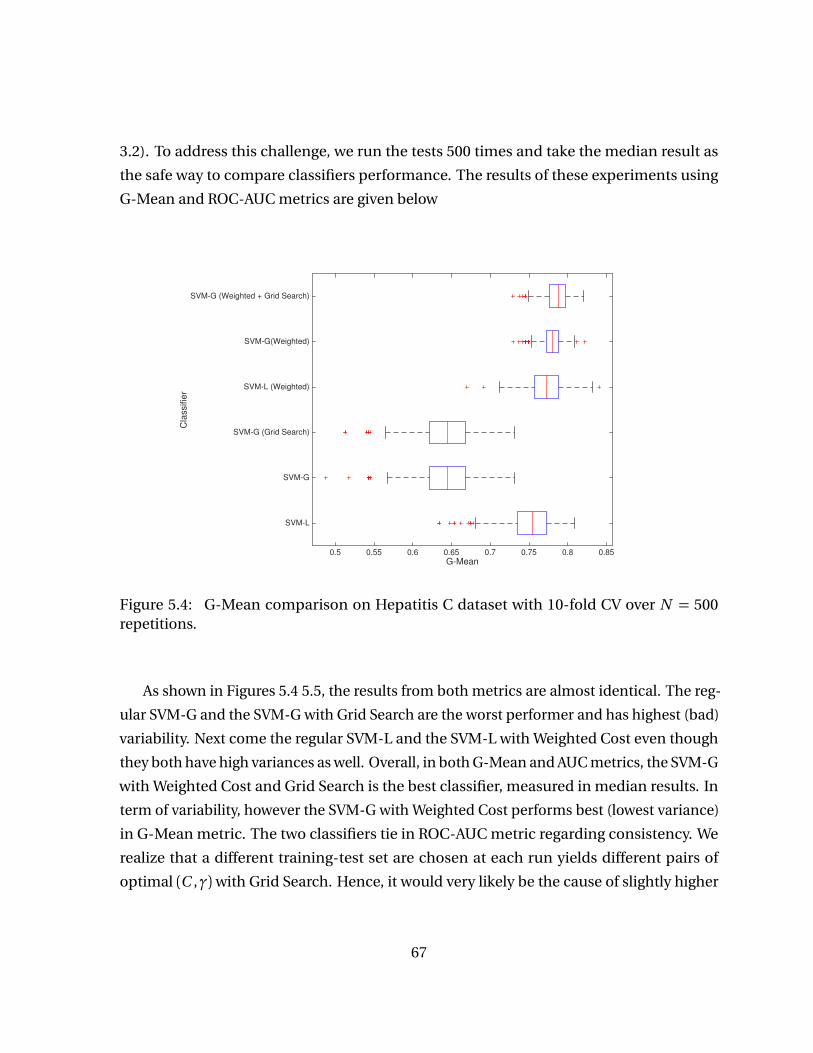
3.2). To address this challenge, we run the tests 500 times and take the median result as

the safe way to compare classifiers performance. The results of these experiments using

G-Mean and ROC-AUC metrics are given below

G-Mean0.5 0.55 0.6 0.65 0.7 0.75 0.8 0.85

Cla

ssifie

r

SVM-L

SVM-G

SVM-G (Grid Search)

SVM-L (Weighted)

SVM-G(Weighted)

SVM-G (Weighted + Grid Search)

Figure 5.4: G-Mean comparison on Hepatitis C dataset with 10-fold CV over N = 500repetitions.

As shown in Figures 5.4 5.5, the results from both metrics are almost identical. The reg-

ular SVM-G and the SVM-G with Grid Search are the worst performer and has highest (bad)

variability. Next come the regular SVM-L and the SVM-L with Weighted Cost even though

they both have high variances as well. Overall, in both G-Mean and AUC metrics, the SVM-G

with Weighted Cost and Grid Search is the best classifier, measured in median results. In

term of variability, however the SVM-G with Weighted Cost performs best (lowest variance)

in G-Mean metric. The two classifiers tie in ROC-AUC metric regarding consistency. We

realize that a different training-test set are chosen at each run yields different pairs of

optimal (C ,γ)with Grid Search. Hence, it would very likely be the cause of slightly higher

67

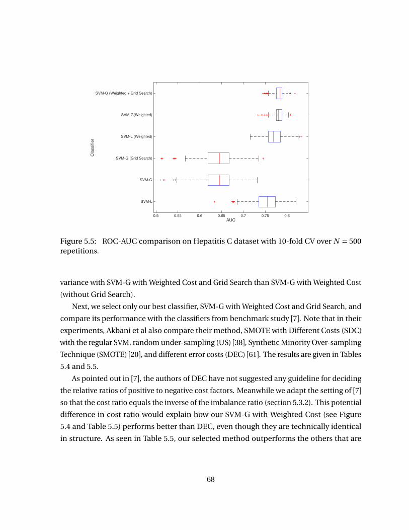
AUC0.5 0.55 0.6 0.65 0.7 0.75 0.8

Cla

ssifie

r

SVM-L

SVM-G

SVM-G (Grid Search)

SVM-L (Weighted)

SVM-G(Weighted)

SVM-G (Weighted + Grid Search)

Figure 5.5: ROC-AUC comparison on Hepatitis C dataset with 10-fold CV over N = 500repetitions.

variance with SVM-G with Weighted Cost and Grid Search than SVM-G with Weighted Cost

(without Grid Search).

Next, we select only our best classifier, SVM-G with Weighted Cost and Grid Search, and

compare its performance with the classifiers from benchmark study [7]. Note that in their

experiments, Akbani et al also compare their method, SMOTE with Different Costs (SDC)

with the regular SVM, random under-sampling (US) [38], Synthetic Minority Over-sampling

Technique (SMOTE) [20], and different error costs (DEC) [61]. The results are given in Tables

5.4 and 5.5.

As pointed out in [7], the authors of DEC have not suggested any guideline for deciding

the relative ratios of positive to negative cost factors. Meanwhile we adapt the setting of [7]

so that the cost ratio equals the inverse of the imbalance ratio (section 5.3.2). This potential

difference in cost ratio would explain how our SVM-G with Weighted Cost (see Figure

5.4 and Table 5.5) performs better than DEC, even though they are technically identical

in structure. As seen in Table 5.5, our selected method outperforms the others that are

68

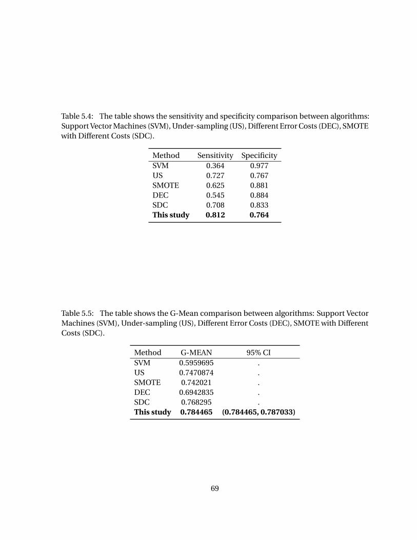
Table 5.4: The table shows the sensitivity and specificity comparison between algorithms:Support Vector Machines (SVM), Under-sampling (US), Different Error Costs (DEC), SMOTEwith Different Costs (SDC).

Method Sensitivity SpecificitySVM 0.364 0.977US 0.727 0.767SMOTE 0.625 0.881DEC 0.545 0.884SDC 0.708 0.833This study 0.812 0.764

Table 5.5: The table shows the G-Mean comparison between algorithms: Support VectorMachines (SVM), Under-sampling (US), Different Error Costs (DEC), SMOTE with DifferentCosts (SDC).

Method G-MEAN 95% CISVM 0.5959695 .US 0.7470874 .SMOTE 0.742021 .DEC 0.6942835 .SDC 0.768295 .This study 0.784465 (0.784465, 0.787033)

69

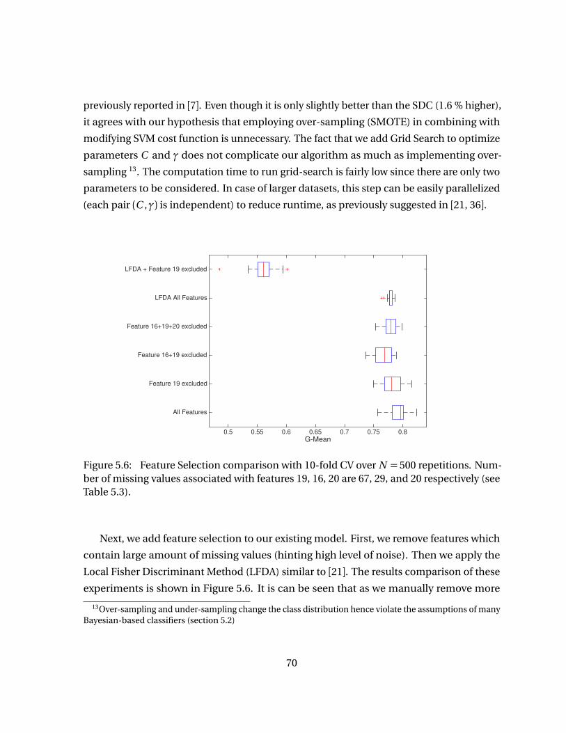
previously reported in [7]. Even though it is only slightly better than the SDC (1.6 % higher),

it agrees with our hypothesis that employing over-sampling (SMOTE) in combining with

modifying SVM cost function is unnecessary. The fact that we add Grid Search to optimize

parameters C and γ does not complicate our algorithm as much as implementing over-

sampling 13. The computation time to run grid-search is fairly low since there are only two

parameters to be considered. In case of larger datasets, this step can be easily parallelized

(each pair (C ,γ) is independent) to reduce runtime, as previously suggested in [21, 36].

G-Mean

0.5 0.55 0.6 0.65 0.7 0.75 0.8

All Features

Feature 19 excluded

Feature 16+19 excluded

Feature 16+19+20 excluded

LFDA All Features

LFDA + Feature 19 excluded

Figure 5.6: Feature Selection comparison with 10-fold CV over N = 500 repetitions. Num-ber of missing values associated with features 19, 16, 20 are 67, 29, and 20 respectively (seeTable 5.3).

Next, we add feature selection to our existing model. First, we remove features which

contain large amount of missing values (hinting high level of noise). Then we apply the

Local Fisher Discriminant Method (LFDA) similar to [21]. The results comparison of these

experiments is shown in Figure 5.6. It is can be seen that as we manually remove more

13Over-sampling and under-sampling change the class distribution hence violate the assumptions of manyBayesian-based classifiers (section 5.2)

70

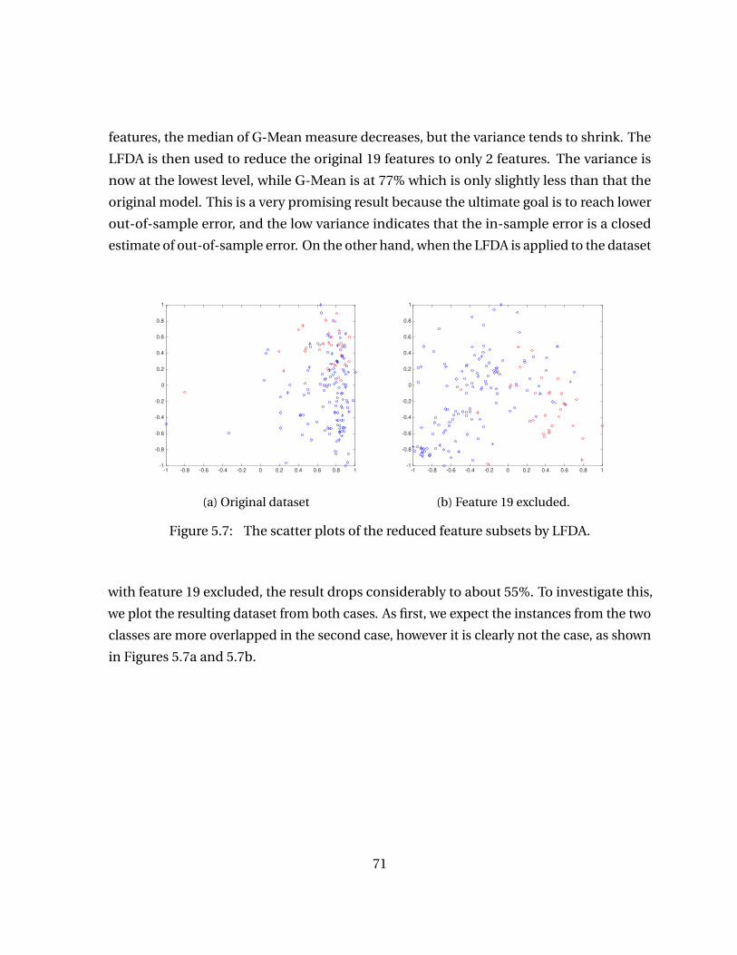
features, the median of G-Mean measure decreases, but the variance tends to shrink. The

LFDA is then used to reduce the original 19 features to only 2 features. The variance is

now at the lowest level, while G-Mean is at 77% which is only slightly less than that the

original model. This is a very promising result because the ultimate goal is to reach lower

out-of-sample error, and the low variance indicates that the in-sample error is a closed

estimate of out-of-sample error. On the other hand, when the LFDA is applied to the dataset

-1 -0.8 -0.6 -0.4 -0.2 0 0.2 0.4 0.6 0.8 1-1

-0.8

-0.6

-0.4

-0.2

0

0.2

0.4

0.6

0.8

1

(a) Original dataset

-1 -0.8 -0.6 -0.4 -0.2 0 0.2 0.4 0.6 0.8 1-1

-0.8

-0.6

-0.4

-0.2

0

0.2

0.4

0.6

0.8

1

(b) Feature 19 excluded.

Figure 5.7: The scatter plots of the reduced feature subsets by LFDA.

with feature 19 excluded, the result drops considerably to about 55%. To investigate this,

we plot the resulting dataset from both cases. As first, we expect the instances from the two

classes are more overlapped in the second case, however it is clearly not the case, as shown

in Figures 5.7a and 5.7b.

71

CHAPTER

6

CONCLUSION AND FUTURE WORK

6.1 Pitch Prediction

In baseball pitch prediction, strong predictive features such as speed and spin rate cannot

be used. This issue forces us to find an innovative way to enhance the quality of the available

feature set. Our research hence revolves around the feature selection step. We highlight

some key contributions below.

• Originally, our approach developed from consideration of the factors that affect

pitching decisions. For example, the pitcher/batter handedness matchup is often

mentioned by sports experts as an effect [31, 35], and was originally included in our

model. However, it was discovered that implementing segmentation of data based on

handedness has essentially no effect on the prediction results. Thus, handedness is no

longer implemented as a further splitting criterion of the model, but this component

remains a considered feature. In general, unnecessary data segmentations have a

72

negative impact solely because they reduce the size of training and testing data for

the classifiers to work with.

• The most notable is our dynamic feature selection approach which widely varies the

set of features used in each pitcher-count situation. Features that yield strong predic-

tion in some situations fail to provide any benefit in others. In fact, it is interesting to

note that in the 2008 vs. 2009 prediction scheme, every feature is used in at least one

situation and no feature is used in every situation. It is also interesting to note that

the LDA, the most successful classification algorithm of this model is supported by

our feature selection technique. In general, as a Bayesian classifier, the LDA relies on

a feature independence assumption, which is realistically not satisfied. Our model

survives this assumption; even though the features within each of the 6 groups are

highly dependent, the final features that are chosen are highly independent.

• The model represents a significant improvement over simple guessing. It is a useful

tool for batting coaches, batters, and others who wish to understand the potential

pitching implications of a given game scenario. For example, batters could theoret-

ically use this model to increase batting average, assuming that knowledge about

a pitch’s type makes it easier to hit. The model, for example, is especially useful in

certain intense game scenarios and achieves accuracy as high as 90 percent. It is in

these game environments that batters can most effectively use this model to translate

knowledge into hits.

Looking forward, much can be done to improve the model.

• First, new features would be helpful. There is much game information that we did

not include in our model, such as batting averages, slugging percentage per batter,

stadium location, weather, and others, which could help improve the prediction

accuracy of the model.

• Another potential modification is extension to multi-class classification. Currently,

our model makes a binary decision and decides if the next pitch will be a fastball or

not. It does not determine what kind of fastball the pitch may be. However, this task

is much more difficult and would almost certainly result in a decrease in accuracy.

73

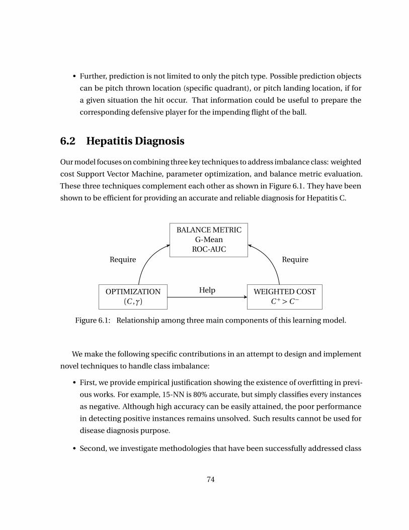
• Further, prediction is not limited to only the pitch type. Possible prediction objects

can be pitch thrown location (specific quadrant), or pitch landing location, if for

a given situation the hit occur. That information could be useful to prepare the

corresponding defensive player for the impending flight of the ball.

6.2 Hepatitis Diagnosis

Our model focuses on combining three key techniques to address imbalance class: weighted

cost Support Vector Machine, parameter optimization, and balance metric evaluation.

These three techniques complement each other as shown in Figure 6.1. They have been

shown to be efficient for providing an accurate and reliable diagnosis for Hepatitis C.

BALANCE METRICG-Mean

ROC-AUC

OPTIMIZATION(C ,γ)

WEIGHTED COSTC + >C −

Help

Require Require

Figure 6.1: Relationship among three main components of this learning model.

We make the following specific contributions in an attempt to design and implement

novel techniques to handle class imbalance:

• First, we provide empirical justification showing the existence of overfitting in previ-

ous works. For example, 15-NN is 80% accurate, but simply classifies every instances

as negative. Although high accuracy can be easily attained, the poor performance

in detecting positive instances remains unsolved. Such results cannot be used for

disease diagnosis purpose.

• Second, we investigate methodologies that have been successfully addressed class

74

imbalance. We design our model by combining the weighted cost SVM with the

parameters optimization via Grid Search. We also replace accuracy by other metrics

such as G-Mean and ROC-AUC that are more appropriate for model evaluation of

unbalanced datasets.

• Finally, learning from small datasets can yield inconsistent results even with cross

validation. In response, we perform 500 simulation runs on our model and use mean

value and 95% confidential interval. This is an attempt to ensure that the result

comparison with the benchmark study is accurate and reliable. Our experiments

show that this model can effectively use the small and unbalanced medical data to

obtain trustworthy diagnosis.

Going forward, we discuss several future research directions as follows.

• Feature selection is a critical step in constructing classifier, it is in fact the center of our

the contribution for the baseball pitch prediction. Our attempt of feature selection

is applying LFDA to reduce the original 19 features to 2 features before feeding in

the classification algorithm. While lower the classification result a little, it greatly en-

hances consistency with noticeable low variance. To enhance classification accuracy,

one potential approach is to determine the right input-output features (currently is

19-2) for LFDA. This is however a tough task against the "Curse of Dimensionality" 1.

• There does not exist a set rule to pre-determine which kernel is best for a given dataset

[1, 6]. In our experiment, we select linear kernel and Gaussian kernel because they

have shown good results and run typically fast. However, authors of [23] introduce

the notion of kernel alignment which indicates the degree of agreement between

a kernel and a given learning task. This notion can potentially be used for kernel

selection. Specifically for unbalanced datasets, the authors of [69] proposed the

conformal transformation kernels. It is interesting to see whether or not this new

class-boundary alignment kernel would interfere with the weighted cost SVM if they

coexist in the same learning algorithm.

1It is common knowledge in machine learning that increasing the number of features increases theaccuracy up to a certain point. Thereafter, it degrades the performance. This phenomenon is referred as the"Curse of Dimensionality"[6].

75

BIBLIOGRAPHY

[1] Abu-Mostafa, Y. S. et al. Learning From Data. AMLBook, 2012.

[2] Adeli, M. & Zarabadipour, H. “Automatic disease diagnosis systems using patternrecognition based genetic algorithm and neural networks”. Int. J. Phys. Sci. v6 i25(2011), pp. 6076–6081.

[3] Adeli, M. et al. “New hybrid hepatitis diagnosis system based on Genetic algorithmand adaptive network fuzzy inference system”. Electrical Engineering (ICEE), 201321st Iranian Conference on. IEEE. 2013, pp. 1–6.

[4] Afif, M. H. et al. “SS-SVM (3SVM): a new classification method for hepatitis diseasediagnosis”. Int. J. Adv. Comput. Sci. Appl 4 (2013).

[5] Akay, M. F. “Support vector machines combined with feature selection for breastcancer diagnosis”. Expert systems with applications 36.2 (2009), pp. 3240–3247.

[6] Akbani, R. Defending against malicious nodes in closed MANETs through packetauthentication and a hybrid trust management system. The University of Texas atSan Antonio, 2009.

[7] Akbani, R. et al. “Applying support vector machines to imbalanced datasets”. MachineLearning: ECML 2004. Springer, 2004, pp. 39–50.

[8] Arlot, S. “A survey of cross-validation procedures for model selection”. StatisticsSurveys 4 (2010), pp. 40–79.

[9] Attarian, A. et al. “A Comparison of Feature Selection and Classification Algorithmsin Identifying Baseball Pitches”. Int. MultiConference of Engineers and ComputerScientists 2013, Lecture Notes in Engineering and Computer Science. NewswoodLimited, 2013, pp. 263–268.

[10] Attarian, A. et al. “Baseball Pitch Classification: A Bayesian Method and Dimension Re-duction Investigation”. IAENG Transactions on Engineering Sciences (2014), pp. 392–399.

[11] Bishop, C. M. “Training with noise is equivalent to Tikhonov regularization”. Neuralcomputation 7.1 (1995), pp. 108–116.

[12] Bishop, C. M. Pattern recognition and machine learning. Springer, 2006.

76

[13] Bradley, A. “The use of the area under the ROC curve in the evaluation of machinelearning algorithms”. Pattern Recogn. 30.7 (1997), pp. 1145–1159.

[14] Burges, C. J. “A tutorial on support vector machines for pattern recognition”. Datamining and knowledge discovery 2.2 (1998), pp. 121–167.

[15] Cawley, G. C. & Talbot, N. L. “Manipulation of prior probabilities in support vectorclassification”. Neural Networks, 2001. Proceedings. IJCNN’01. International JointConference on. Vol. 4. IEEE. 2001, pp. 2433–2438.

[16] Central, H. What is Ascites? URL: http://www.hepatitiscentral.com/hcv/whatis/ascites/.

[17] Chabacano. Diagram showing overfitting of a classifier. 2008. URL:https://commons.wikimedia.org/wiki/File:Overfitting.svg.

[18] Chang, C.-C. & Lin, C.-J. “LIBSVM: A library for support vector machines”. ACMTransactions on Intelligent Systems and Technology (TIST) 2.3 (2011), p. 27.

[19] Chang, C.-C. & Lin, C.-J. “LIBSVM: A library for support vector machines”. ACMTransactions on Intelligent Systems and Technology 2 (3 2011). Software available athttp://www.csie.ntu.edu.tw/~cjlin/libsvm, 27:1–27:27.

[20] Chawla, N. V. et al. “SMOTE: synthetic minority over-sampling technique”. Journal ofartificial intelligence research (2002), pp. 321–357.

[21] Chen, H.-L. et al. “A new hybrid method based on local fisher discriminant analysisand support vector machines for hepatitis disease diagnosis”. Expert Systems withApplications 38.9 (2011), pp. 11796–11803.

[22] Courant, R. & Hilbert, D. Methods of mathematical physics. Vol. 1. CUP Archive, 1966.

[23] CRISTIANINI, N. “On kernel-target alignment”. Advances in Neural InformationProcessing Systems (2002).

[24] Delen, D. et al. “Predicting breast cancer survivability: a comparison of three datamining methods”. Artificial intelligence in medicine 34.2 (2005), pp. 113–127.

[25] Drummond, C. & Holte, R. C. “Exploiting the cost (in) sensitivity of decision treesplitting criteria”. ICML. 2000, pp. 239–246.

[26] Duch, W. et al. “Minimal distance neural methods” (1998).

77

[27] Efron, B. “Estimating the error rate of a prediction rule: improvement on cross-validation”. Journal of the American Statistical Association 78.382 (1983), pp. 316–331.

[28] Egan, J. Signal detection theory and ROC analysis. New York: Cognition and Percep-tion. Academic Press, 1975.

[29] Elkan, C. “The foundations of cost-sensitive learning”. International joint conferenceon artificial intelligence. Vol. 17. 1. Citeseer. 2001, pp. 973–978.

[30] Fawcett, T. “An introduction to ROC analysis”. Pattern recognition letters 27.8 (2006),pp. 861–874.

[31] Ganeshapillai, G. & Guttag, J. “Predicting the Next Pitch”. MIT Sloan Sports AnalyticsConference. 2012.

[32] Hamilton, M. et al. “Applying Machine Learning Techniques to Baseball Pitch Predic-tion”. 3rd Int. Conf. on Pattern Recognition Applications and Methods. SciTePress,2014, pp. 520–527.

[33] Hastie, T. & Tibshirani, R. The elements of statistical learning. Springer, 2009.

[34] He, H., Garcia, E., et al. “Learning from imbalanced data”. Knowledge and DataEngineering, IEEE Transactions on 21.9 (2009), pp. 1263–1284.

[35] Hopkins, T. & Magel, R. “Slugging Percentage in Differing Baseball Counts”. Journalof Quantitative Analysis in Sports 4.2 (2008), p. 1136.

[36] Hsu, C.-W. et al. A practical guide to support vector classification. 2003.

[37] James, G. et al. An introduction to statistical learning. Springer, 2013.

[38] Japkowicz, N. “The class imbalance problem: Significance and strategies”. Proc. ofthe Int. Conf. on Artificial Intelligence. Citeseer. 2000.

[39] Jerez-Aragonés, J. M. et al. “A combined neural network and decision trees model forprognosis of breast cancer relapse”. Artificial intelligence in medicine 27.1 (2003),pp. 45–63.

[40] Jilani, T. A. et al. “PCA-ANN for classification of Hepatitis-C patients”. InternationalJournal of Computer Applications (0975–8887) 14.7 (2011).

78

[41] Karabatak, M. & Ince, M. C. “An expert system for detection of breast cancer based onassociation rules and neural network”. Expert Systems with Applications 36.2 (2009),pp. 3465–3469.

[42] Kubat, M., Matwin, S., et al. “Addressing the curse of imbalanced training sets: one-sided selection”. ICML. Vol. 97. Nashville, USA. 1997, pp. 179–186.

[43] Kubat, M. et al. “Learning when negative examples abound”. Machine learning:ECML-97. Springer, 1997, pp. 146–153.

[44] Lichman, M. UCI Machine Learning Repository. 2013.

[45] Lin, Y. et al. “Support vector machines for classification in nonstandard situations”.Machine learning 46.1-3 (2002), pp. 191–202.

[46] Marckmann, G. “Recommendations for the ethical development and use of medicaldecision-support systems.” MedGenMed: Medscape general medicine 3.3 (2001),pp. 5–5.

[47] Neshat, M. & Yaghobi, M. “Designing a fuzzy expert system of diagnosing the hep-atitis B intensity rate and comparing it with adaptive neural network fuzzy system”.Proceedings of the World Congress on Engineering and Computer Science. Vol. 2.2009, pp. 797–802.

[48] Ng, A. Y. “Feature selection, L 1 vs. L 2 regularization, and rotational invariance”.Proceedings of the twenty-first international conference on Machine learning. ACM.2004, p. 78.

[49] Nugroho, A. S. et al. “A solution for imbalanced training sets problem by combnet-iiand its application on fog forecasting”. IEICE TRANSACTIONS on Information andSystems 85.7 (2002), pp. 1165–1174.

[50] Peng, Y. Tikz example-Kernel trick. 2013. URL: http://blog.pengyifan.com/tikz-example-kernel-trick/.

[51] Peng, Y. Tikz example-SVM trained with samples from two classes. 2013. URL:http://blog.pengyifan.com/tikz-example-svm-trained-with-samples-from-two-classes/.

[52] Polat, K. & Günes, S. “Breast cancer diagnosis using least square support vectormachine”. Digital Signal Processing 17.4 (2007), pp. 694–701.

79

[53] Provost, F. “Machine learning from imbalanced data sets 101”. Proceedings of theAAAI 2000 workshop on imbalanced data sets. 2000, pp. 1–3.

[54] Sahan, S. et al. “A new hybrid method based on fuzzy-artificial immune system andk-nn algorithm for breast cancer diagnosis”. Computers in Biology and Medicine37.3 (2007), pp. 415–423.

[55] Smola, A. J. et al. “The connection between regularization operators and supportvector kernels”. Neural networks 11.4 (1998), pp. 637–649.

[56] Swets, J. et al. “Better decisions through science”. Scientific American 283 (2000),pp. 82–87.

[57] Theodoridis, S. & Koutroumbas, K. Pattern recognition. 4th. Burlington, Mass.: Aca-demic Press, 2009.

[58] Thoma, M. Normal distribution for a discriminant analysis. 2014. URL: https://commons.wikimedia.org/wiki/File:Lda-gauss-1.svg#globalusage.

[59] Vapnik, V. The nature of statistical learning theory. Springer Science & Business Media,2013.

[60] Vapnik, V. N. “An overview of statistical learning theory”. Neural Networks, IEEETransactions on 10.5 (1999), pp. 988–999.

[61] Veropoulos, K. et al. “Controlling the sensitivity of support vector machines”. Pro-ceedings of the international joint conference on AI. 1999, pp. 55–60.

[62] Veterans Affirs, U. D. of. Viral Hepatitis: Commonly used terms in cirrhosis. URL:http://www.hepatitis.va.gov/patient/complications/cirrhosis/terms.asp.

[63] Wang, B. X. & Japkowicz, N. “Boosting support vector machines for imbalanced datasets”. Knowledge and Information Systems 25.1 (2010), pp. 1–20.

[64] Wang, S.-j. et al. “Empirical analysis of support vector machine ensemble classifiers”.Expert Systems with Applications 36.3 (2009), pp. 6466–6476.

[65] Weinstein-Gould, J. “Keeping the Hitter Off Balance: Mixed Strategies in Baseball”.Journal of Quantitative Analysis in Sports 5.2 (2009), p. 1173.

80

[66] West, D. & West, V. “Model selection for a medical diagnostic decision support system:a breast cancer detection case”. Artificial Intelligence in medicine 20.3 (2000), pp. 183–204.

[67] West, D. et al. “Ensemble strategies for a medical diagnostic decision support system:A breast cancer diagnosis application”. European Journal of Operational Research162.2 (2005), pp. 532–551.

[68] Wikipedia. Wikipedia Glossary of Baseball. 2013. URL:http://en.wikipedia.org/wiki/Glossary-of-baseball.

[69] Wu, G. & Chang, E. Y. “Class-boundary alignment for imbalanced dataset learning”.ICML 2003 workshop on learning from imbalanced data sets II, Washington, DC.2003, pp. 49–56.

[70] Xue, J.-H. & Hall, P. “Why Does Rebalancing Class-unbalanced Data Improve AUCfor Linear Discriminant Analysis?” Pattern Analysis and Machine Intelligence, IEEETransactions on 37.5 (2015), pp. 1109–1112.

[71] Yasin, H. et al. “Hepatitis-C classification using data mining techniques”. Interna-tional Journal of Computer Applications 24.3 (2011), pp. 1–6.

[72] Zweig, M. H. & Campbell, G. “Receiver-operating characteristic ROC plots: A fun-damental evaluation tool in clinical medicine”. Clin. Chem. 39.4 (1993), pp. 561–577.

81

APPENDICES

82

APPENDIX

A

BASEBALL PITCH PREDICTION

A.1 Features in Groups

From the original 18 features given in Table 4.1, we generated a total of 77 features and

arranged them into 6 groups as follows:

Group 1: General information of game situation

1. Inning

2. Time (day/afternoon/night)

3. Number of outs

4. Last at bat events

5. Pitcher vs. batter specific: fastball or nonfastball on previous pitch

83

6. Pitcher vs. batter specific: lifetime percentage of fastballs

7. Pitcher vs. batter specific: previous pitch’s events

8. Numeric score of previous at bat event

9. Player on first base (true/false)

10. Player on second base (true/false)

11. Player on third base (true/false)

12. Number of base runners

13. Weighted base score

Group 2: Pitch type tendency from the past

1. Percentage of fastball thrown in previous inning

2. Percentage of fastball thrown in previous game

3. Percentage of fastballs thrown in previous at bat

4. Lifetime percentage of fastballs thrown to a specific batter over all at bats

5. Percentage of fastballs over previous 5 pitches

6. Percentage of fastballs over previous 10 pitches

7. Percentage of fastballs over previous 15 pitches

8. Percentage of fastballs over previous 20 pitches

9. Previous pitch in specific count: pitch type

10. Previous pitch in specific count: fastball or nonfastball

11. Previous 2 pitches in specific count: fastball/nonfastball combo

84

12. Previous 3 pitches in specific count: fastball/nonfastball combo

13. Previous pitch: pitch type

14. Previous pitch: fastball or nonfastball

15. Previous 2 pitches: fastball/nonfastball combo

16. Inning

17. Player on first base (true/false)

18. Percentage of fastballs over previous 10 pitches thrown to a specific batter

19. Percentage of fastballs over previous 15 pitches thrown to a specific batter

20. Previous 5 pitches in specific count: percentage of fastballs

21. Previous 10 pitches in specific count: percentage of fastballs

22. Previous 15 pitches in specific count: percentage of fastballs

Group 3: Pitch velocity from the past

1. Previous pitch: velocity

2. Previous 2 pitches: velocity average

3. Previous 3 pitches: velocity average

4. Previous pitch in specific count: velocity

5. Previous 2 pitches in specific count: velocity average

6. Previous 3 pitches in specific count: velocity average

85

Group 4: Pitch location at home plate

1. Previous pitch: horizontal position

2. Previous pitch: vertical position

3. Previous 2 pitches: horizontal position average

4. Previous 2 pitches: vertical position average

5. Previous 3 pitches: horizontal position average

6. Previous 3 pitches: vertical position average

7. Previous pitch: zone (Cartesian quadrant)

8. Previous 2 pitches: zone (Cartesian quadrant) average

9. Previous 3 pitches: zone (Cartesian quadrant) average

10. Previous pitch in specific count: horizontal position

11. Previous pitch in specific count: vertical position

12. Previous 2 pitches in specific count: horizontal position average

13. Previous 2 pitches in specific count: vertical position average

14. Previous 3 pitches in specific count: horizontal position average

15. Previous 3 pitches in specific count: vertical position average

16. Previous pitch in specific count: zone (Cartesian quadrant)

17. Previous 2 pitches in specific count: zone (Cartesian quadrant) average

18. Previous 3 pitches in specific count: zone (Cartesian quadrant) average

86

Group 5: Strike-result-percentage

Strike-result percentage (SRP): a metric we created that measures the percentage of strikes

from all pitches in the given situation.

1. SRP of fastball thrown in the previous inning

2. SRP of fastball thrown in the previous game

3. SRP of fastball thrown in the previous 5 pitches

4. SRP of fastball thrown in the previous 10 pitches

5. SRP of fastball thrown in the previous 15 pitches

6. SRP of fastball thrown in previous 5 pitches thrown to the currently facing batter

7. SRP of nonfastball thrown in the previous inning

8. SRP of nonfastball thrown in the previous game

9. SRP of nonfastball thrown in the previous 5 pitches

10. SRP of nonfastball thrown in the previous 10 pitches

11. SRP of nonfastball thrown in the previous 15 pitches

12. SRP of nonfastball thrown in previous 5 pitches thrown to the currently facing batter

Group 6: Ball-strike combo from the similar count in the past

1. Previous pitch: ball or strike (boolean)

2. Previous 2 pitches: ball/strike combo

3. Previous 3 pitches: ball/strike combo

4. Previous pitch in specific count: ball or strike

5. Previous 2 pitches in specific count: ball/strike combo

6. Previous 3 pitches in specific count: ball/strike combo

87

A.2 Baseball Glossary and Info

Most of these definitions are obtained directly from [68].

1. Strike Zone: A box over the home plate which defines the boundaries through which

a pitch must pass in order to count as a strike when the batter does not swing. A pitch

that does not cross the plate through the strike zone is a ball.

2. Strike: When a batter swings at a pitch but fails to hit it, when a batter does not swing

at a pitch that is thrown within the strike zone, when the ball is hit foul and the strike

count is less than 2 (a batter cannot strike out on a foul ball, however he can fly out),

when a ball is bunted foul, regardless of the strike count, when the ball touches the

batter as he swings at it, when the ball touches the batter in the strike zone, or when

the ball is a foul tip. Three strikes and the batter is said to have struck out.

3. Ball: When the batter does not swing at the pitch and the pitch is outside the strike

zone. If the batter accrues four balls in an at bat he gets a walk, a free pass to first

base.

4. Hit-By-Pitch: When the pitch hits the batters body. The batter gets a free pass to first

base, similar to a walk.

5. Hit: When the batter makes contact with the pitch and successfully reaches first,

second or third base. Types of hits include single (batter ends at first base), doubles

(batter ends at second base), triple (batter ends at third base) and home-run.

6. Out: When a batter or base runner cannot, for whatever reason, advance to the next

base. Examples include striking out (batter can not advance to first), grounding out,

popping out and lining out.

7. Count: Is the number of balls and strikes during an at bat. There are 12 possible

counts spanning every combination of 0-3 balls (4 balls is a walk) and 0-2 strikes (3

strikes is a strikeout).

88

8. Run: When a base runner crosses home plate. This is a point for that player’s team.

The outcome of a baseball game is determined by which team has more runs at the

end of nine Innings.

9. Inning: One of nine periods of playtime in a standard game.

10. Slugging Percentage: A measure of hitter power. Defined as the average number of

bases the hitter earns per at bat.

11. Batting Average: The percentage of time the batter earns a hit.

12. At Bat : A series of pitches thrown by the pitcher to one hitter resulting in a hit, a walk,

or an out.

A.3 Software

All data processing and classification tasks were preformed off-line using commercial

software package MATLAB (R2014a), The MathWorks Inc., Natick, MA.

1. k -NN(s, c): k -nearest-neighbors algorithm (MATLAB: knnsearch) with standardized

Euclidean metric/Manhattan metric

2. SVM (L, G): Support Vector Machine with linear kernel and with Gaussian kernel

3. LDA: Linear discriminant analysis (MATLAB: classify) with linear and quadratic types.

89

APPENDIX

B

HEPATITIS C DIAGNOSIS

B.1 Definitions of Attributes

1. Steroid: Any group of lipids with a specific 7 carbon atom ring system [71].

2. Antiviral: It’s a drug that inhibits the viral effects [71].

3. Fatigue: A state of increased discomfort and decreased efficiency due to prolonged

or excessive exertion [71].

4. Malaise: Feeling of discomfort [71].

5. Anorexia: Lack or loss of appetite for foods [71].

6. Liver Big: Liver increased in size or fatty liver [71].

7. Liver Firm: Irregular hardness of liver [71].

90

8. Spleen Palpable: This symptom usually occur when the liver is questionably enlarged

[16].

9. Spiders: Tiny veins that look like little red spiders on face, chest, and arms. They are

signs of cirrhosis [62].

10. Ascites: The presence of excess fluid in the peritoneal cavity [16].

11. Bilirubin: A yellowish substance that is created by the breakdown (destruction) of

hemoglobin, a major component of red blood cells [62].

12. Alk Phosphate: An enzyme exists in the blood [40].

13. Varices: Enlarged veins in the esophagus that can burst open and lead to vomiting

blood or having black stool [40].

14. SGOT: Serum glutamic oxaloacetic transaminase (SGOT) is an enzyme generally exists

in serum. Also, it is present in the heart [40].

15. Albumin: The chief protein of blood plasma as well as other serous solutions [40].

16. PROTIME: Prothrombin is a predecessor of thrombin which is produced in the liver

[40].

91