Rigging the Lottery: Making All Tickets Winners

Utku Evci 1 Trevor Gale 1 Jacob Menick 2 Pablo Samuel Castro 1 Erich Elsen 2

Abstract Many applications require sparse neural networks due to space or inference time restrictions. There is a large body of work on training dense networks to yield sparse networks for inference, but this lim-its the size of the largest trainable sparse model to that of the largest trainable dense model. In this paper we introduce a method to train sparse neural networks with a fixed parameter count and a fixed computational cost throughout training, without sacrificing accuracy relative to existing dense-to-sparse training methods. Our method updates the topology of the sparse network during training by using parameter magnitudes and infrequent gra-dient calculations. We show that this approach requires fewer floating-point operations (FLOPs) to achieve a given level of accuracy compared to prior techniques. We demonstrate state-of-the-art sparse training results on a variety of networks and datasets, including ResNet-50, MobileNets on Imagenet-2012, and RNNs on WikiText-103. Fi-nally, we provide some insights into why allowing the topology to change during the optimization can overcome local minima encountered when the topology remains static*.

1. Introduction

The parameter and floating point operation (FLOP) effi-ciency of sparse neural networks is now well demonstrated on a variety of problems (Han et al., 2015; Srinivas et al., 2017). Multiple works have shown inference time speedups are possible using sparsity for both Recurrent Neural Net-works (RNNs) (Kalchbrenner et al., 2018) and Convolu-tional Neural Networks (ConvNets) (Park et al., 2016; Elsen et al., 2019). Currently, the most accurate sparse models

1Google Brain 2DeepMind. Correspondence to: Utku Evci <evcu@google.com>, Erich Elsen <eriche@google.com>.

Proceedings of the 37 th International Conference on Machine Learning, Vienna, Austria, PMLR 119, 2020. Copyright 2020 by the author(s).

*Code available at github.com/google-research/rigl

Figure 1. RigL improves the optimization of sparse neural net-works by leveraging weight magnitude and gradient information to jointly optimize model parameters and connectivity.

are obtained with techniques that require, at a minimum, the cost of training a dense model in terms of memory and FLOPs (Zhu & Gupta, 2018; Guo et al., 2016), and some-times significantly more (Molchanov et al., 2017).

This paradigm has two main limitations. First, the maximum size of sparse models is limited to the largest dense model that can be trained; even if sparse models are more parameter efficient, we can’t use pruning to train models that are larger and more accurate than the largest possible dense models. Second, it is inefficient; large amounts of computation must be performed for parameters that are zero valued or that will be zero during inference. Additionally, it remains unknown if the performance of the current best pruning algorithms is an upper bound on the quality of sparse models. Gale et al. (2019) found that three different dense-to-sparse training algorithms all achieve about the same sparsity / accuracy trade-off. However, this is far from conclusive proof that no better performance is possible.

The Lottery Ticket Hypothesis (Frankle & Carbin, 2019) hypothesized that if we can find a sparse neural network with iterative pruning, then we can train that sparse network from scratch, to the same level of accuracy, by starting from

Rigging the Lottery: Making All Tickets Winners

the original initial conditions. In this paper we introduce a new method for training sparse models without the need of a “lucky” initialization; for this reason, we call our method “The Rigged Lottery” or RigL†. We make the following specific contributions:

• We introduce RigL - an algorithm for training sparse neural networks while maintaining memory and com-putational cost proportional to density of the network.

• We perform an extensive empirical evaluation of RigL on computer vision and natural language tasks. We show that RigL achieves higher quality than all previ-ous techniques for a given computational cost.

• We show the surprising result that RigL can find more accurate models than the current best dense-to-sparse training algorithms.

• We study the loss landscape of sparse neural networks and provide insight into why allowing the topology of nonzero weights to change over the course of training aids optimization.

2. Related Work

Research on finding sparse neural networks dates back decades, at least to Thimm & Fiesler (1995) who concluded that pruning weights based on magnitude was a simple and powerful technique. Strom (1997) later introduced the idea of retraining the previously pruned network to increase ac-curacy. Han et al. (2016b) went further and introduced multiple rounds of magnitude pruning and retraining. This is, however, relatively inefficient, requiring ten rounds of retraining when removing 20% of the connections to reach a final sparsity of 90%. To overcome this problem, Narang et al. (2017) introduced gradual pruning, where connec-tions are slowly removed over the course of a single round of training. Zhu & Gupta (2018) refined the technique to minimize the amount of hyper-parameter selection required.

A diversity of approaches not based on magnitude pruning have also been proposed. Mozer & Smolensky (1989), Le-Cun et al. (1990) and Hassibi & Stork (1993) are some early examples, but impractical for modern neural networks as they use information from the Hessian to prune a trained net-work. More recent work includes L0 Regularization (Chris-tos Louizos, 2018), Variational Dropout (Molchanov et al., 2017), Dynamic Network Surgery (Guo et al., 2016), Dis-covering Neural Wirings (Wortsman et al., 2019), Sensitiv-ity Driven Regularization (Tartaglione et al., 2018). Gale et al. (2019) examined magnitude pruning, L0 Regulariza-tion, and Variational Dropout and concluded that they all

†Pronounced ”wriggle”.

achieve about the same accuracy versus sparsity trade-off on ResNet-50 and Transformer architectures.

There are also structured pruning methods which attempt to remove channels or neurons so that the resulting network is dense and can be accelerated easily (Dai et al., 2018; Nek-lyudov et al., 2017; Christos Louizos, 2018). We compare RigL with these state-of-the-art structured pruning meth-ods in Appendix B. We show that our method requires far fewer resources and finds smaller networks that require less FLOPs to run.

Training techniques that allow for sparsity throughout the entire training process were, to our knowledge, first intro-duced in Deep Rewiring (DeepR) (Bellec et al., 2018). In DeepR, the standard Stochastic Gradient Descent (SGD) optimizer is augmented with a random walk in parameter space. Additionally, at initialization connections are as-signed a pre-defined sign at random; when the optimizer would normally flip the sign, the weight is set to 0 instead and new weights are activated at random.

Sparse Evolutionary Training (SET) (Mocanu et al., 2018) proposed a simpler scheme where weights are pruned ac-cording to the standard magnitude criterion used in prun-ing and are added back at random. The method is simple and achieves reasonable performance in practice. Dynamic Sparse Reparameterization (DSR) (Mostafa & Wang, 2019) introduced the idea of allowing the parameter budget to shift between different layers of the model, allowing for non-uniform sparsity. This allows the model to distribute parameters where they are most effective. Unfortunately, the models under consideration are mostly convolutional networks, so the result of this parameter reallocation (which is to decrease the sparsity of early layers and increase the sparsity of later layers) has the overall effect of increasing the FLOP count because the spatial size is largest in the early layers. Sparse Networks from Scratch (SNFS) (Dettmers & Zettlemoyer, 2019) introduces the idea of using the momen-tum of each parameter as the criterion to be used for growing weights and demonstrates it leads to an improvement in test accuracy. Like DSR, they allow the sparsity of each layer to change and focus on a constant parameter, not FLOP, budget. Importantly, the method requires computing gra-dients and updating the momentum for every parameter in the model, even those that are zero, at every iteration. This can result in a significant amount of overall computation. Additionally, depending on the model and training setup, the required storage for the full momentum tensor could be prohibitive. Single-Shot Network Pruning (SNIP) (Lee et al., 2019) attempts to find an initial mask with one-shot pruning and uses the saliency score of parameters to decide which parameters to keep. After pruning, training proceeds with this static sparse network. Properties of the different sparse training techniques are summarized in Table 1.

�

�

�

�

�

Rigging the Lottery: Making All Tickets Winners

Method Drop Grow Selectable FLOPs Space & FLOPs / SNIP

DeepR SET DSR SNFS

RigL (ours)

min(|✓ ⇤ r✓L(✓)|) stochastic min(|✓|) min(|✓|) min(|✓|) min(|✓|)

none random random random

momentum gradient

yes yes yes no no yes

sparse sparse sparse sparse dense sparse

Table 1. Comparison of different sparse training techniques. Drop and Grow columns correspond to the strategies used during the mask update. Selectable FLOPs is possible if the cost of training the model is fixed at the beginning of training.

There has also been a line of work investigating the Lot-tery Ticket Hypothesis (Frankle & Carbin, 2019). Frankle et al. (2019) showed that the formulation must be weakened to apply to larger networks such as ResNet-50 (He et al., 2015). In large networks, instead of the original initializa-tion, the values after thousands of optimization steps must be used for initialization. (Zhou et al., 2019) showed that ”winning lottery tickets” obtain non-random accuracies even before training has started. Though the possibility of train-ing sparse neural networks with a fixed sparsity mask using lottery tickets is intriguing, it remains unclear whether it is possible to generate such initializations – for both masks and parameters – de novo.

3. Rigging The Lottery

Our method, RigL, is illustrated in Figure 1 and detailed in Algorithm 1. RigL starts with a random sparse network, and at regularly spaced intervals it removes a fraction of con-nections based on their magnitudes and activates new ones using instantaneous gradient information. After updating the connectivity, training continues with the updated net-work until the next update. The main parts of our algorithm, Sparsity Distribution, Update Schedule, Drop Criterion, Grow Criterion, and the various options considered for each, are explained below.

(0) Notation. Given a dataset D with individual samples xi and targets yi, we aim to minimize the loss functionP

i L(f⇥(xi), yi), where f⇥(·) is a neural network with pa-rameters ⇥ 2 RN . Parameters of the lth layer are denoted with ⇥l which is a length N l vector. A sparse layer keeps only a fraction sl 2 (0, 1) of its connections and parameter-ized with vector ✓l of length (1 sl)N l . Parameters of the corresponding sparse network is denoted with ✓. Finally, the overall sparsity of a sparse network is defined as the ratio ofP

zeros to the total parameter count, i.e. S = l s l N l

N

(1) Sparsity Distribution. There are many ways of dis-tributing the non-zero weights across the layers while main-taining a certain overall sparsity. We avoid re-allocating parameters between layers during the training process as it makes it difficult to target a specific final FLOP budget,

which is important for many applications. We consider the following three strategies:

1. Uniform: The sparsity sl of each individual layer is equal to the total sparsity S. In this setting, we keep the first layer dense, since sparsifying this layer has a disproportional effect on the performance and almost no effect on the total size.

2. Erd˝ enyi: As introduced in (Mocanu et al., 2018),os-R´ l-1 l n +nsl scales with 1 , where nl denotes number nl-1⇤nl

of neurons at layer l. This enables the number of con-nections in a sparse layer to scale with the sum of the number of output and input channels.

3. Erd˝ enyi-Kernel (ERK): This method modifies the os-R´ original Erdos-Renyi formulation by including the ker-´ nel dimensions in the scaling factors. In other words, the number of parameters of the sparse convolutional

l-1 l l n +n +w +hl

layers are scaled proportional to 1 ,nl-1⇤nl⇤wl⇤hl

where wl and hl are the width and the height of the l’th convolutional kernel. Sparsity of the fully connected layers scale as in the original Erdos-Renyi formulation.´ Similar to Erdos-Renyi, ERK allocates higher sparsi-´ ties to the layers with more parameters while allocating lower sparsities to the smaller ones.

In all methods, the bias and batch-norm parameters are kept dense, since these parameters scale with total number of neurons and have a negligible effect on the total model size.

(2) Update Schedule. The update schedule is defined by the following parameters: (1) T : the number of iterations between sparse connectivity updates, (2) Tend: the iteration at which to stop updating the sparse connectivity, (3) ↵: the initial fraction of connections updated and (4) fdecay: a function, invoked every T iterations until Tend, possibly decaying the fraction of updated connections over time. For the latter, as in Dettmers & Zettlemoyer (2019), we use cosine annealing, as we find it slightly outperforms the other methods considered.

✓ ✓ ◆◆ ↵ t⇡

fdecay (t; ↵, Tend) = 1 + cos 2 Tend

�� �

� �

�

�

�

��

�

�

Rigging the Lottery: Making All Tickets Winners

Results obtained with other annealing functions, such as constant and inverse power, are presented in Appendix G.

(3) Drop criterion. Every T steps we drop the con-nections given by ArgTopK( |✓l|, (1 sl)N l), where ArgTopK(v, k) gives the indices of the top-k elements of vector v.

(4) Grow criterion. The novelty of our method lies in how we grow new connections. We grow the connections with highest magnitude gradients, ArgTopKi/ (|r⇥l Lt|, k), where ✓l \ Idrop is the 2✓l\Idrop

set of active connections remaining after step (3). Newly activated connections are initialized to zero and therefore don’t affect the output of the network. However they are ex-pected to receive gradients with high magnitudes in the next iteration and therefore reduce the loss fastest. We attempted using other initialization like random values or small values along the gradient direction for the activated connections, however zero initialization brought the best results.

This procedure can be applied to each layer in sequence and the dense gradients can be discarded immediately after selecting the top connections. If a layer is too large to store the full gradient with respect to the weights, then the gra-dients can be calculated in an online manner and only the

1top-k gradient values are stored. As long as T > , the 1 s extra work of calculating dense gradients is amortized and still proportional to 1 S. This is in contrast to the method of (Dettmers & Zettlemoyer, 2019), which requires calculat-ing and storing the full gradients at each optimization step.

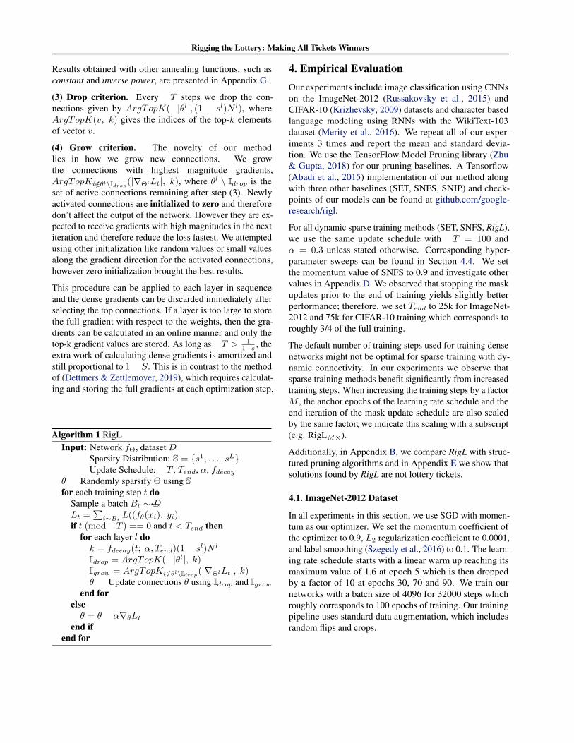
Algorithm 1 RigL Input: Network f⇥, dataset D

1Sparsity Distribution: S = {s , . . . , sL} Update Schedule: T , Tend, ↵, fdecay

✓ Randomly sparsify ⇥ using S for each training step t do

Sample a batch Bt ⇠ DP Lt = L((f✓(xi), yi)i⇠Bt

if t (mod T ) == 0 and t < Tend then for each layer l do k = fdecay(t; ↵, Tend)(1 sl)N l

Idrop = ArgTopK( |✓l|, k) Igrow = ArgTopKi/ (|r⇥l Lt|, k)2✓l \Idrop

✓ Update connections ✓ using Idrop and Igrow

end for else ✓ = ✓ ↵r✓Lt

end if end for

4. Empirical Evaluation

Our experiments include image classification using CNNs on the ImageNet-2012 (Russakovsky et al., 2015) and CIFAR-10 (Krizhevsky, 2009) datasets and character based language modeling using RNNs with the WikiText-103 dataset (Merity et al., 2016). We repeat all of our exper-iments 3 times and report the mean and standard devia-tion. We use the TensorFlow Model Pruning library (Zhu & Gupta, 2018) for our pruning baselines. A Tensorflow (Abadi et al., 2015) implementation of our method along with three other baselines (SET, SNFS, SNIP) and check-points of our models can be found at github.com/google-research/rigl.

For all dynamic sparse training methods (SET, SNFS, RigL), we use the same update schedule with T = 100 and ↵ = 0.3 unless stated otherwise. Corresponding hyper-parameter sweeps can be found in Section 4.4. We set the momentum value of SNFS to 0.9 and investigate other values in Appendix D. We observed that stopping the mask updates prior to the end of training yields slightly better performance; therefore, we set Tend to 25k for ImageNet-2012 and 75k for CIFAR-10 training which corresponds to roughly 3/4 of the full training.

The default number of training steps used for training dense networks might not be optimal for sparse training with dy-namic connectivity. In our experiments we observe that sparse training methods benefit significantly from increased training steps. When increasing the training steps by a factor M , the anchor epochs of the learning rate schedule and the end iteration of the mask update schedule are also scaled by the same factor; we indicate this scaling with a subscript (e.g. RigLM⇥).

Additionally, in Appendix B, we compare RigL with struc-tured pruning algorithms and in Appendix E we show that solutions found by RigL are not lottery tickets.

4.1. ImageNet-2012 Dataset

In all experiments in this section, we use SGD with momen-tum as our optimizer. We set the momentum coefficient of the optimizer to 0.9, L2 regularization coefficient to 0.0001, and label smoothing (Szegedy et al., 2016) to 0.1. The learn-ing rate schedule starts with a linear warm up reaching its maximum value of 1.6 at epoch 5 which is then dropped by a factor of 10 at epochs 30, 70 and 90. We train our networks with a batch size of 4096 for 32000 steps which roughly corresponds to 100 epochs of training. Our training pipeline uses standard data augmentation, which includes random flips and crops.

�

Rigging the Lottery: Making All Tickets Winners

Method Top-1 Accuracy

FLOPs (Train)

FLOPs (Test)

Top-1 Accuracy

FLOPs (Train)

FLOPs (Test)

Dense 76.8±0.09 1x (3.2e18)

1x (8.2e9)

S=0.8 S=0.9

Static 70.6±0.06 0.23x 0.23x 65.8±0.04 0.10x 0.10x SNIP 72.0±0.10 0.23x 0.23x 67.2±0.12 0.10x 0.10x

Small-Dense 72.1±0.12 0.20x 0.20x 68.9±0.10 0.12x 0.12x SET 72.9±0.39 0.23x 0.23x 69.6±0.23 0.10x 0.10x RigL 74.6±0.06 0.23x 0.23x 72.0±0.05 0.10x 0.10x

Small-Dense5⇥ 73.9±0.07 1.01x 0.20x 71.3±0.10 0.60x 0.12x RigL5⇥ 76.6±0.06 1.14x 0.23x 75.7±0.06 0.52x 0.10x

Static (ERK) 72.1±0.04 0.42x 0.42x 67.7±0.12 0.24x 0.24x DSR* 73.3 0.40x 0.40x 71.6 0.30x 0.30x

RigL (ERK) 75.1±0.05 0.42x 0.42x 73.0±0.04 0.25x 0.24x RigL5⇥ (ERK) 77.1±0.06 2.09x 0.42x 76.4±0.05 1.23x 0.24x

SNFS* 74.2 n/a n/a 72.3 n/a n/a SNFS (ERK) 75.2±0.11 0.61x 0.42x 72.9±0.06 0.50x 0.24x

Pruning* 75.6 0.56x 0.23x 73.9 0.51x 0.10x Pruning1.5⇥ * 76.5 0.84x 0.23x 75.2 0.76x 0.10x

DNW* 76 n/a n/a 74 n/a n/a

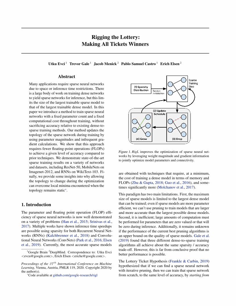
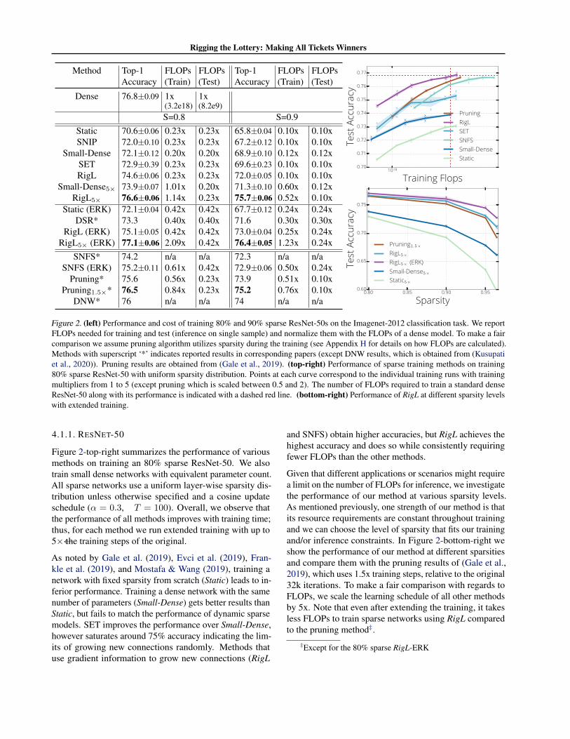
Figure 2. (left) Performance and cost of training 80% and 90% sparse ResNet-50s on the Imagenet-2012 classification task. We report FLOPs needed for training and test (inference on single sample) and normalize them with the FLOPs of a dense model. To make a fair comparison we assume pruning algorithm utilizes sparsity during the training (see Appendix H for details on how FLOPs are calculated). Methods with superscript ‘*’ indicates reported results in corresponding papers (except DNW results, which is obtained from (Kusupati et al., 2020)). Pruning results are obtained from (Gale et al., 2019). (top-right) Performance of sparse training methods on training 80% sparse ResNet-50 with uniform sparsity distribution. Points at each curve correspond to the individual training runs with training multipliers from 1 to 5 (except pruning which is scaled between 0.5 and 2). The number of FLOPs required to train a standard dense ResNet-50 along with its performance is indicated with a dashed red line. (bottom-right) Performance of RigL at different sparsity levels with extended training.

4.1.1. RESNET-50

Figure 2-top-right summarizes the performance of various methods on training an 80% sparse ResNet-50. We also train small dense networks with equivalent parameter count. All sparse networks use a uniform layer-wise sparsity dis-tribution unless otherwise specified and a cosine update schedule (↵ = 0.3, T = 100). Overall, we observe that the performance of all methods improves with training time; thus, for each method we run extended training with up to 5⇥ the training steps of the original.

As noted by Gale et al. (2019), Evci et al. (2019), Fran-kle et al. (2019), and Mostafa & Wang (2019), training a network with fixed sparsity from scratch (Static) leads to in-ferior performance. Training a dense network with the same number of parameters (Small-Dense) gets better results than Static, but fails to match the performance of dynamic sparse models. SET improves the performance over Small-Dense, however saturates around 75% accuracy indicating the lim-its of growing new connections randomly. Methods that use gradient information to grow new connections (RigL

and SNFS) obtain higher accuracies, but RigL achieves the highest accuracy and does so while consistently requiring fewer FLOPs than the other methods.

Given that different applications or scenarios might require a limit on the number of FLOPs for inference, we investigate the performance of our method at various sparsity levels. As mentioned previously, one strength of our method is that its resource requirements are constant throughout training and we can choose the level of sparsity that fits our training and/or inference constraints. In Figure 2-bottom-right we show the performance of our method at different sparsities and compare them with the pruning results of (Gale et al., 2019), which uses 1.5x training steps, relative to the original 32k iterations. To make a fair comparison with regards to FLOPs, we scale the learning schedule of all other methods by 5x. Note that even after extending the training, it takes less FLOPs to train sparse networks using RigL compared to the pruning method‡.

‡Except for the 80% sparse RigL-ERK

Rigging the Lottery: Making All Tickets Winners

S Method Top-1 FLOPs

0.75 Small-Dense5⇥

Pruning (Zhu) RigL5⇥

RigL5⇥ (ERK)

66.0±0.11 67.7

71.5±0.06 71.9±0.01

0.23x 0.27x 0.27x 0.52x

0.9 Small-Dense5⇥

Pruning (Zhu) RigL5⇥

RigL5⇥ (ERK)

57.7±0.34 61.8

67.0±0.17 68.1±0.11

0.09x 0.12x 0.12x 0.27x

Dense 72.1±0.17 1x (1.1e9)

0.75 Big-Sparse5⇥

Big-Sparse5⇥ (ERK) 76.4±0.05 77.0±0.08

0.98x 1.91x

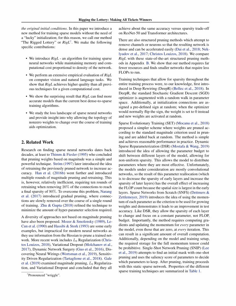
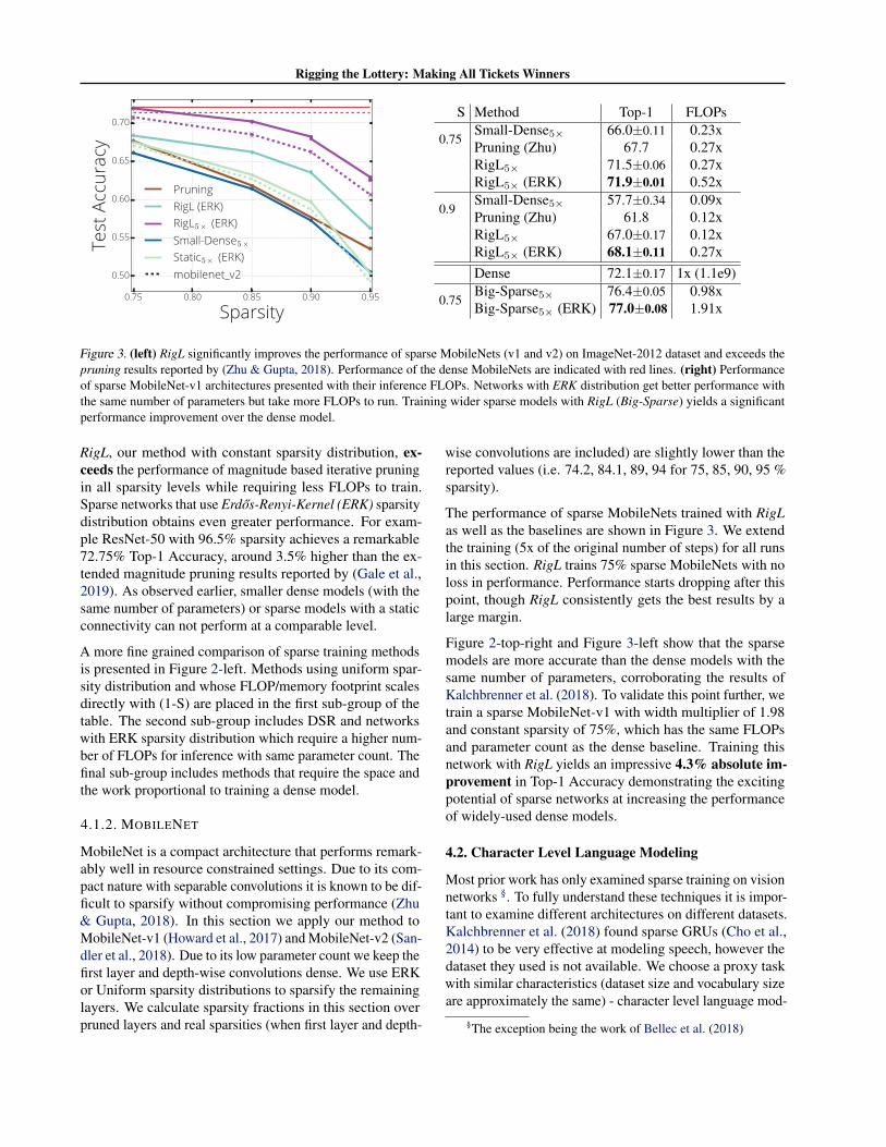
Figure 3. (left) RigL significantly improves the performance of sparse MobileNets (v1 and v2) on ImageNet-2012 dataset and exceeds the pruning results reported by (Zhu & Gupta, 2018). Performance of the dense MobileNets are indicated with red lines. (right) Performance of sparse MobileNet-v1 architectures presented with their inference FLOPs. Networks with ERK distribution get better performance with the same number of parameters but take more FLOPs to run. Training wider sparse models with RigL (Big-Sparse) yields a significant performance improvement over the dense model.

RigL, our method with constant sparsity distribution, ex-ceeds the performance of magnitude based iterative pruning in all sparsity levels while requiring less FLOPs to train. Sparse networks that use Erdos-Renyi-Kernel (ERK) sparsity distribution obtains even greater performance. For exam-ple ResNet-50 with 96.5% sparsity achieves a remarkable 72.75% Top-1 Accuracy, around 3.5% higher than the ex-tended magnitude pruning results reported by (Gale et al., 2019). As observed earlier, smaller dense models (with the same number of parameters) or sparse models with a static connectivity can not perform at a comparable level.

A more fine grained comparison of sparse training methods is presented in Figure 2-left. Methods using uniform spar-sity distribution and whose FLOP/memory footprint scales directly with (1-S) are placed in the first sub-group of the table. The second sub-group includes DSR and networks with ERK sparsity distribution which require a higher num-ber of FLOPs for inference with same parameter count. The final sub-group includes methods that require the space and the work proportional to training a dense model.

4.1.2. MOBILENET

MobileNet is a compact architecture that performs remark-ably well in resource constrained settings. Due to its com-pact nature with separable convolutions it is known to be dif-ficult to sparsify without compromising performance (Zhu & Gupta, 2018). In this section we apply our method to MobileNet-v1 (Howard et al., 2017) and MobileNet-v2 (San-dler et al., 2018). Due to its low parameter count we keep the first layer and depth-wise convolutions dense. We use ERK or Uniform sparsity distributions to sparsify the remaining layers. We calculate sparsity fractions in this section over

wise convolutions are included) are slightly lower than the reported values (i.e. 74.2, 84.1, 89, 94 for 75, 85, 90, 95 % sparsity).

The performance of sparse MobileNets trained with RigL as well as the baselines are shown in Figure 3. We extend the training (5x of the original number of steps) for all runs in this section. RigL trains 75% sparse MobileNets with no loss in performance. Performance starts dropping after this point, though RigL consistently gets the best results by a large margin.

Figure 2-top-right and Figure 3-left show that the sparse models are more accurate than the dense models with the same number of parameters, corroborating the results of Kalchbrenner et al. (2018). To validate this point further, we train a sparse MobileNet-v1 with width multiplier of 1.98 and constant sparsity of 75%, which has the same FLOPs and parameter count as the dense baseline. Training this network with RigL yields an impressive 4.3% absolute im-provement in Top-1 Accuracy demonstrating the exciting potential of sparse networks at increasing the performance of widely-used dense models.

4.2. Character Level Language Modeling

Most prior work has only examined sparse training on vision networks §. To fully understand these techniques it is impor-tant to examine different architectures on different datasets. Kalchbrenner et al. (2018) found sparse GRUs (Cho et al., 2014) to be very effective at modeling speech, however the dataset they used is not available. We choose a proxy task with similar characteristics (dataset size and vocabulary size are approximately the same) - character level language mod-

pruned layers and real sparsities (when first layer and depth- §The exception being the work of Bellec et al. (2018)

�

Rigging the Lottery: Making All Tickets Winners

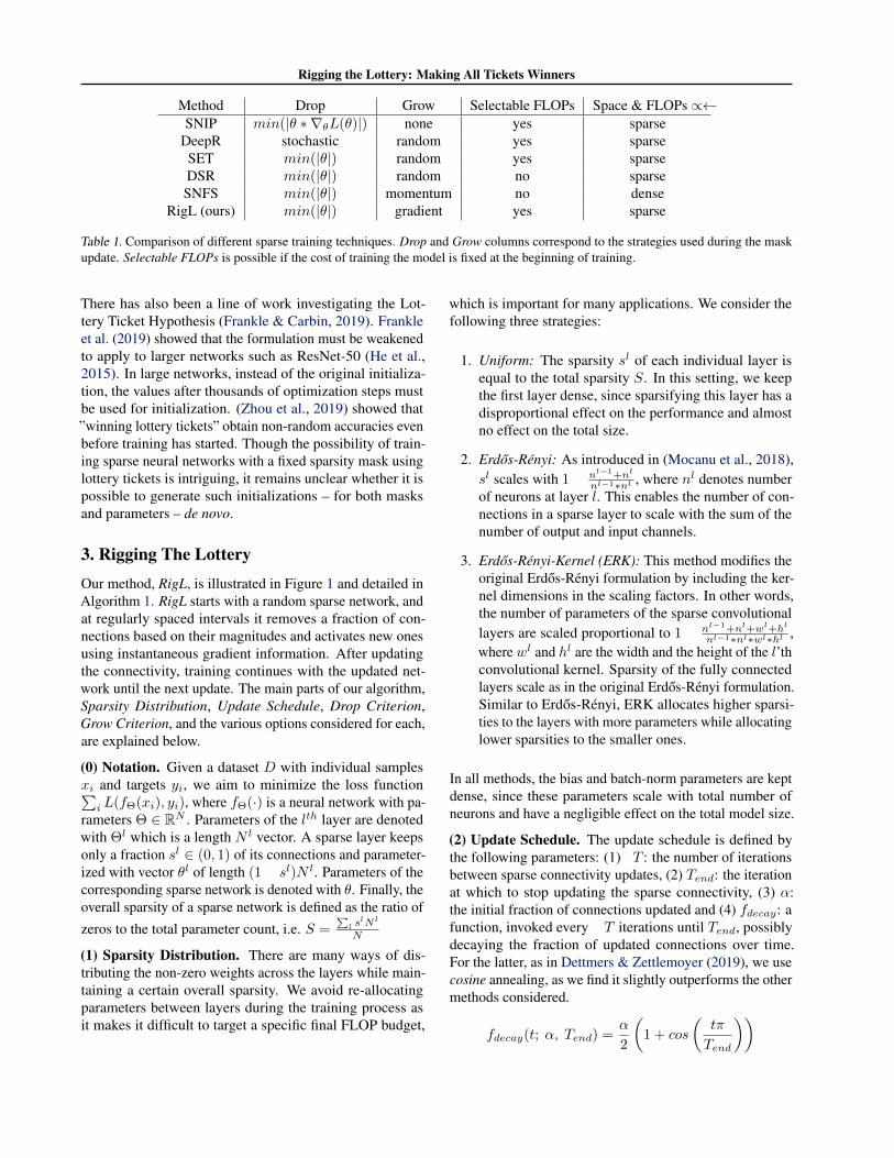
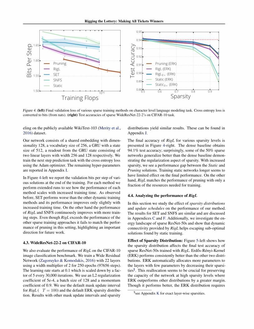
Figure 4. (left) Final validation loss of various sparse training methods on character level language modeling task. Cross entropy loss is converted to bits (from nats). (right) Test accuracies of sparse WideResNet-22-2’s on CIFAR-10 task.

eling on the publicly available WikiText-103 (Merity et al., 2016) dataset.

Our network consists of a shared embedding with dimen-sionality 128, a vocabulary size of 256, a GRU with a state size of 512, a readout from the GRU state consisting of two linear layers with width 256 and 128 respectively. We train the next step prediction task with the cross entropy loss using the Adam optimizer. The remaining hyper-parameters are reported in Appendix I.

In Figure 4-left we report the validation bits per step of vari-ous solutions at the end of the training. For each method we perform extended runs to see how the performance of each method scales with increased training time. As observed before, SET performs worse than the other dynamic training methods and its performance improves only slightly with increased training time. On the other hand the performance of RigL and SNFS continuously improves with more train-ing steps. Even though RigL exceeds the performance of the other sparse training approaches it fails to match the perfor-mance of pruning in this setting, highlighting an important direction for future work.

4.3. WideResNet-22-2 on CIFAR-10

We also evaluate the performance of RigL on the CIFAR-10 image classification benchmark. We train a Wide Residual Network (Zagoruyko & Komodakis, 2016) with 22 layers using a width multiplier of 2 for 250 epochs (97656 steps). The learning rate starts at 0.1 which is scaled down by a fac-tor of 5 every 30,000 iterations. We use an L2 regularization coefficient of 5e-4, a batch size of 128 and a momentum coefficient of 0.9. We use the default mask update interval for RigL ( T = 100) and the default ERK sparsity distribu-tion. Results with other mask update intervals and sparsity

distributions yield similar results. These can be found in Appendix J.

The final accuracy of RigL for various sparsity levels is presented in Figure 4-right. The dense baseline obtains 94.1% test accuracy; surprisingly, some of the 50% sparse networks generalize better than the dense baseline demon-strating the regularization aspect of sparsity. With increased sparsity, we see a performance gap between the Static and Pruning solutions. Training static networks longer seems to have limited effect on the final performance. On the other hand, RigL matches the performance of pruning with only a fraction of the resources needed for training.

4.4. Analyzing the performance of RigL

In this section we study the effect of sparsity distributions and update schedules on the performance of our method. The results for SET and SNFS are similar and are discussed in Appendices C and F. Additionally, we investigate the en-ergy landscape of sparse ResNet-50s and show that dynamic connectivity provided by RigL helps escaping sub-optimal solutions found by static training.

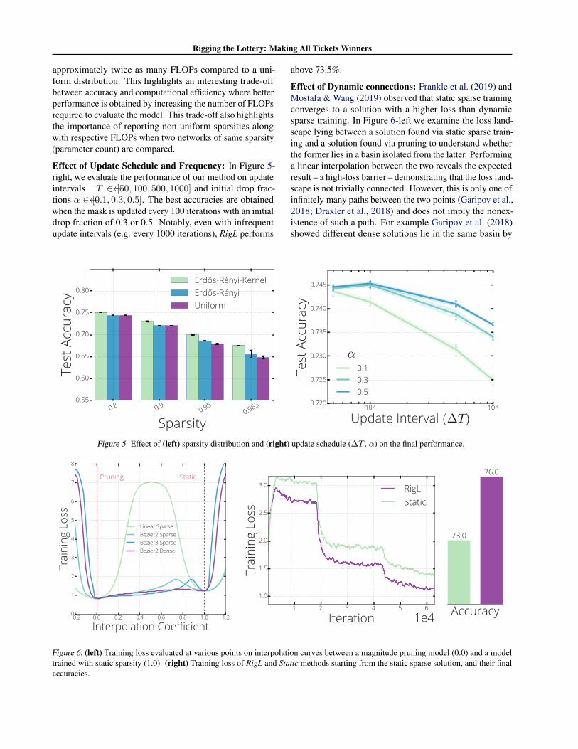
Effect of Sparsity Distribution: Figure 5-left shows how the sparsity distribution affects the final test accuracy of sparse ResNet-50s trained with RigL. Erdos-Renyi-Kernel´ (ERK) performs consistently better than the other two distri-butions. ERK automatically allocates more parameters to the layers with few parameters by decreasing their sparsi-ties¶. This reallocation seems to be crucial for preserving the capacity of the network at high sparsity levels where ERK outperforms other distributions by a greater margin. Though it performs better, the ERK distribution requires

¶see Appendix K for exact layer-wise sparsities.

�

Rigging the Lottery: Making All Tickets Winners

approximately twice as many FLOPs compared to a uni-form distribution. This highlights an interesting trade-off between accuracy and computational efficiency where better performance is obtained by increasing the number of FLOPs required to evaluate the model. This trade-off also highlights the importance of reporting non-uniform sparsities along with respective FLOPs when two networks of same sparsity (parameter count) are compared.

Effect of Update Schedule and Frequency: In Figure 5-right, we evaluate the performance of our method on update intervals T 2 [50, 100, 500, 1000] and initial drop frac-tions ↵ 2 [0.1, 0.3, 0.5]. The best accuracies are obtained when the mask is updated every 100 iterations with an initial drop fraction of 0.3 or 0.5. Notably, even with infrequent update intervals (e.g. every 1000 iterations), RigL performs

above 73.5%.

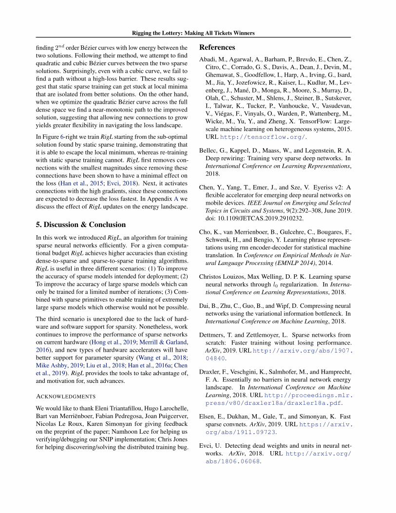
Effect of Dynamic connections: Frankle et al. (2019) and Mostafa & Wang (2019) observed that static sparse training converges to a solution with a higher loss than dynamic sparse training. In Figure 6-left we examine the loss land-scape lying between a solution found via static sparse train-ing and a solution found via pruning to understand whether the former lies in a basin isolated from the latter. Performing a linear interpolation between the two reveals the expected result – a high-loss barrier – demonstrating that the loss land-scape is not trivially connected. However, this is only one of infinitely many paths between the two points (Garipov et al., 2018; Draxler et al., 2018) and does not imply the nonex-istence of such a path. For example Garipov et al. (2018) showed different dense solutions lie in the same basin by

Figure 5. Effect of (left) sparsity distribution and (right) update schedule (�T , ↵) on the final performance.

Figure 6. (left) Training loss evaluated at various points on interpolation curves between a magnitude pruning model (0.0) and a model trained with static sparsity (1.0). (right) Training loss of RigL and Static methods starting from the static sparse solution, and their final accuracies.

Rigging the Lottery: Making All Tickets Winners

finding 2nd order Bezier curves with low energy between the two solutions. Following their method, we attempt to find quadratic and cubic Bezier curves between the two sparse solutions. Surprisingly, even with a cubic curve, we fail to find a path without a high-loss barrier. These results sug-gest that static sparse training can get stuck at local minima that are isolated from better solutions. On the other hand, when we optimize the quadratic Bezier curve across the full dense space we find a near-monotonic path to the improved solution, suggesting that allowing new connections to grow yields greater flexibility in navigating the loss landscape.

In Figure 6-right we train RigL starting from the sub-optimal solution found by static sparse training, demonstrating that it is able to escape the local minimum, whereas re-training with static sparse training cannot. RigL first removes con-nections with the smallest magnitudes since removing these connections have been shown to have a minimal effect on the loss (Han et al., 2015; Evci, 2018). Next, it activates connections with the high gradients, since these connections are expected to decrease the loss fastest. In Appendix A we discuss the effect of RigL updates on the energy landscape.

5. Discussion & Conclusion

In this work we introduced RigL, an algorithm for training sparse neural networks efficiently. For a given computa-tional budget RigL achieves higher accuracies than existing dense-to-sparse and sparse-to-sparse training algorithms. RigL is useful in three different scenarios: (1) To improve the accuracy of sparse models intended for deployment; (2) To improve the accuracy of large sparse models which can only be trained for a limited number of iterations; (3) Com-bined with sparse primitives to enable training of extremely large sparse models which otherwise would not be possible.

The third scenario is unexplored due to the lack of hard-ware and software support for sparsity. Nonetheless, work continues to improve the performance of sparse networks on current hardware (Hong et al., 2019; Merrill & Garland, 2016), and new types of hardware accelerators will have better support for parameter sparsity (Wang et al., 2018; Mike Ashby, 2019; Liu et al., 2018; Han et al., 2016a; Chen et al., 2019). RigL provides the tools to take advantage of, and motivation for, such advances.

ACKNOWLEDGMENTS

We would like to thank Eleni Triantafillou, Hugo Larochelle, Bart van Merrienboer, Fabian Pedregosa, Joan Puigcerver, Nicolas Le Roux, Karen Simonyan for giving feedback on the preprint of the paper; Namhoon Lee for helping us verifying/debugging our SNIP implementation; Chris Jones for helping discovering/solving the distributed training bug.

References

Abadi, M., Agarwal, A., Barham, P., Brevdo, E., Chen, Z., Citro, C., Corrado, G. S., Davis, A., Dean, J., Devin, M., Ghemawat, S., Goodfellow, I., Harp, A., Irving, G., Isard, M., Jia, Y., Jozefowicz, R., Kaiser, L., Kudlur, M., Lev-enberg, J., Mane, D., Monga, R., Moore, S., Murray, D., Olah, C., Schuster, M., Shlens, J., Steiner, B., Sutskever, I., Talwar, K., Tucker, P., Vanhoucke, V., Vasudevan, V., Viegas, F., Vinyals, O., Warden, P., Wattenberg, M., Wicke, M., Yu, Y., and Zheng, X. TensorFlow: Large-scale machine learning on heterogeneous systems, 2015. URL http://tensorflow.org/.

Bellec, G., Kappel, D., Maass, W., and Legenstein, R. A. Deep rewiring: Training very sparse deep networks. In International Conference on Learning Representations, 2018.

Chen, Y., Yang, T., Emer, J., and Sze, V. Eyeriss v2: A flexible accelerator for emerging deep neural networks on mobile devices. IEEE Journal on Emerging and Selected Topics in Circuits and Systems, 9(2):292–308, June 2019. doi: 10.1109/JETCAS.2019.2910232.

Cho, K., van Merrienboer, B., Gulcehre, C., Bougares, F., Schwenk, H., and Bengio, Y. Learning phrase represen-tations using rnn encoder-decoder for statistical machine translation. In Conference on Empirical Methods in Nat-ural Language Processing (EMNLP 2014), 2014.

Christos Louizos, Max Welling, D. P. K. Learning sparse neural networks through l0 regularization. In Interna-tional Conference on Learning Representations, 2018.

Dai, B., Zhu, C., Guo, B., and Wipf, D. Compressing neural networks using the variational information bottleneck. In International Conference on Machine Learning, 2018.

Dettmers, T. and Zettlemoyer, L. Sparse networks from scratch: Faster training without losing performance. ArXiv, 2019. URL http://arxiv.org/abs/1907. 04840.

Draxler, F., Veschgini, K., Salmhofer, M., and Hamprecht, F. A. Essentially no barriers in neural network energy landscape. In International Conference on Machine Learning, 2018. URL http://proceedings.mlr. press/v80/draxler18a/draxler18a.pdf.

Elsen, E., Dukhan, M., Gale, T., and Simonyan, K. Fast sparse convnets. ArXiv, 2019. URL https://arxiv. org/abs/1911.09723.

Evci, U. Detecting dead weights and units in neural net-works. ArXiv, 2018. URL http://arxiv.org/ abs/1806.06068.

Rigging the Lottery: Making All Tickets Winners

Evci, U., Pedregosa, F., Gomez, A. N., and Elsen, E. The difficulty of training sparse neural networks. ArXiv, 2019. URL http://arxiv.org/abs/1906.10732.

Frankle, J. and Carbin, M. The lottery ticket hypothe-sis: Finding sparse, trainable neural networks. In In-ternational Conference on Learning Representations, 2019. URL https://openreview.net/forum? id=rJl-b3RcF7.

Frankle, J., Dziugaite, G. K., Roy, D. M., and Carbin, M. The lottery ticket hypothesis at scale. ArXiv, 2019. URL http://arxiv.org/abs/1903.01611.

Gale, T., Elsen, E., and Hooker, S. The state of sparsity in deep neural networks. ArXiv, 2019. URL http: //arxiv.org/abs/1902.09574.

Garipov, T., Izmailov, P., Podoprikhin, D., Vetrov, D. P., and Wilson, A. G. Loss surfaces, mode connectivity, and fast ensembling of dnns. In Advances in Neural Information Processing Systems, 2018.

Guo, Y., Yao, A., and Chen, Y. Dynamic network surgery for efficient DNNs. ArXiv, 2016. URL http://arxiv. org/abs/1608.04493.

Han, S., Pool, J., Tran, J., and Dally, W. Learning both weights and connections for efficient neural network. In Advances in Neural Information Processing Systems, 2015.

Han, S., Liu, X., Mao, H., Pu, J., Pedram, A., Horowitz, M. A., and Dally, W. J. EIE: Efficient Inference Engine on compressed deep neural network. In Proceedings of the 43rd International Symposium on Computer Architecture, 2016a.

Han, S., Mao, H., and Dally, W. J. Deep compression: Compressing deep neural network with pruning, trained quantization and huffman coding. In International Con-ference on Learning Representations, 2016b. URL http://arxiv.org/abs/1510.00149.

Hassibi, B. and Stork, D. Second order derivatives for network pruning: Optimal Brain Surgeon. In Advances in Neural Information Processing Systems, 1993.

He, K., Zhang, X., Ren, S., and Sun, J. Delving deep into rectifiers: Surpassing human-level performance on imagenet classification. In Proceedings of the 2015 IEEE International Conference on Computer Vision (ICCV), 2015.

Hong, C., Sukumaran-Rajam, A., Nisa, I., Singh, K., and Sadayappan, P. Adaptive sparse tiling for sparse ma-trix multiplication. In Proceedings of the 24th Sym-posium on Principles and Practice of Parallel Pro-

gramming, 2019. URL http://doi.acm.org/10. 1145/3293883.3295712.

Howard, A. G., Zhu, M., Chen, B., Kalenichenko, D., Wang, W., Weyand, T., Andreetto, M., and Adam, H. Mobilenets: Efficient convolutional neural networks for mobile vision applications. ArXiv, 2017. URL http: //arxiv.org/abs/1704.04861.

Kalchbrenner, N., Elsen, E., Simonyan, K., Noury, S., Casagrande, N., Lockhart, E., Stimberg, F., Oord, A., Dieleman, S., and Kavukcuoglu, K. Efficient neural au-dio synthesis. In International Conference on Machine Learning, 2018.

Krizhevsky, A. Learning multiple layers of fea-tures from tiny images. In University of Toronto, 2009. URL https://www.cs.toronto.edu/ ˜kriz/learning-features-2009-TR.pdf.

Kusupati, A., Ramanujan, V., Somani, R., Wortsman, M., Jain, P., Kakade, S., and Farhadi, A. Soft threshold weight reparameterization for learnable sparsity. In International Conference on Machine Learning, 2020.

LeCun, Y., Denker, J. S., and Solla, S. A. Optimal Brain Damage. In Advances in Neural Information Processing Systems, 1990.

Lee, N., Ajanthan, T., and Torr, P. H. S. SNIP: Single-shot Network Pruning based on Connection Sensitivity. In International Conference on Learning Representations, 2019.

Liu, C., Bellec, G., Vogginger, B., Kappel, D., Partzsch, J., Neumaerker, F., Hoppner, S., Maass, W., Furber, S. B., Legenstein, R. A., and Mayr, C. Memory-efficient deep learning on a spinnaker 2 prototype. In Front. Neurosci., 2018.

Liu, Z., Sun, M., Zhou, T., Huang, G., and Darrell, T. Re-thinking the value of network pruning. In International Conference on Learning Representations, 2019.

Merity, S., Xiong, C., Bradbury, J., and Socher, R. Pointer sentinel mixture models. ArXiv, 2016. URL http: //arxiv.org/abs/1609.07843.

Merrill, D. and Garland, M. Merge-based sparse matrix-vector multiplication (spmv) using the csr storage for-mat. In Proceedings of the 21st ACM SIGPLAN Sym-posium on Principles and Practice of Parallel Pro-gramming, 2016. URL http://doi.acm.org/10. 1145/2851141.2851190.

Mike Ashby, Christiaan Baaij, P. B. M. B. O. B. A. C. C. C. L. C. S. D. N. v. D. J. F. G. H. B. H. D. P. J.

Rigging the Lottery: Making All Tickets Winners

S. S. S. Exploiting unstructured sparsity on next-generation datacenter hardware. 2019. URL https:// myrtle.ai/wp-content/uploads/2019/06/ IEEEformatMyrtle.ai_.21.06.19_b.pdf.

Mocanu, D. C., Mocanu, E., Stone, P., Nguyen, P. H., Gibescu, M., and Liotta, A. Scalable training of ar-tificial neural networks with adaptive sparse connec-tivity inspired by network science. Nature Communi-cations, 2018. URL http://www.nature.com/ articles/s41467-018-04316-3.

Molchanov, D., Ashukha, A., and Vetrov, D. P. Variational Dropout Sparsifies Deep Neural Networks. In Interna-tional Conference on Machine Learning, pp. 2498–2507, 2017.

Molchanov, P., Tyree, S., Karras, T., Aila, T., and Kautz, J. Pruning Convolutional Neural Networks for Resource Efficient Transfer Learning. ArXiv, 2016. URL https: //arxiv.org/abs/1611.06440.

Mostafa, H. and Wang, X. Parameter efficient training of deep convolutional neural networks by dynamic sparse reparameterization. In International Conference on Ma-chine Learning, 2019. URL http://proceedings. mlr.press/v97/mostafa19a.html.

Mozer, M. C. and Smolensky, P. Skeletonization: A tech-nique for trimming the fat from a network via relevance assessment. In Advances in Neural Information Process-ing Systems, 1989.

Narang, S., Diamos, G., Sengupta, S., and Elsen, E. Ex-ploring sparsity in recurrent neural networks. In In-ternational Conference on Learning Representations, 2017. URL https://openreview.net/forum? id=BylSPv9gx.

Neklyudov, K., Molchanov, D., Ashukha, A., and Vetrov, D. Structured bayesian pruning via log-normal multiplicative noise. In Advances in Neural Information Processing Systems, 2017.

Park, J., Li, S. R., Wen, W., Li, H., Chen, Y., and Dubey, P. Holistic SparseCNN: Forging the trident of accuracy, speed, and size. ArXiv, 2016. URL http://arxiv. org/abs/1608.01409.

Russakovsky, O., Deng, J., Su, H., Krause, J., Satheesh, S., Ma, S., Huang, Z., Karpathy, A., Khosla, A., Bernstein, M., Berg, A. C., and Fei-Fei, L. Imagenet large scale visual recognition challenge. International Journal of Computer Vision (IJCV), 2015.

Sandler, M., Howard, A., Zhu, M., Zhmoginov, A., and Chen, L. Mobilenetv2: Inverted residuals and linear bottlenecks. In 2018 IEEE/CVF Conference on Computer Vision and Pattern Recognition, 2018.

Srinivas, S., Subramanya, A., and Babu, R. V. Training sparse neural networks. In 2017 IEEE Conference on Computer Vision and Pattern Recognition Workshops (CVPRW), 2017.

Strom, N. Sparse Connection and Pruning in Large Dynamic Artificial Neural Networks. In EUROSPEECH, 1997.

Szegedy, C., Vanhoucke, V., Ioffe, S., Shlens, J., and Wojna, Z. Rethinking the inception architecture for computer vision. In Proceedings of IEEE Conference on Computer Vision and Pattern Recognition,, 2016. URL http:// arxiv.org/abs/1512.00567.

Tartaglione, E., Lepsøy, S., Fiandrotti, A., and Francini, G. Learning sparse neural networks via sensitivity-driven regularization. In Advances in Neural Information Pro-cessing Systems, 2018. URL http://dl.acm.org/ citation.cfm?id=3327144.3327303.

Thimm, G. and Fiesler, E. Evaluating pruning methods. In Proceedings of the International Symposium on Artificial Neural Networks, 1995.

Wang, P., Ji, Y., Hong, C., Lyu, Y., Wang, D., and Xie, Y. Snrram: An efficient sparse neural network computation architecture based on resistive random-access memory. In Proceedings of the 55th Annual Design Automation Conference, 2018. URL http://doi.acm.org/10. 1145/3195970.3196116.

Wortsman, M., Farhadi, A., and Rastegari, M. Discovering neural wirings. ArXiv, 2019. URL http://arxiv. org/abs/1906.00586.

Zagoruyko, S. and Komodakis, N. Wide residual networks. In British Machine Vision Conference, 2016. URL http://www.bmva.org/bmvc/2016/ papers/paper087/index.html.

Zhou, H., Lan, J., Liu, R., and Yosinski, J. Deconstruct-ing lottery tickets: Zeros, signs, and the supermask. ArXiv, 2019. URL http://arxiv.org/abs/1905. 01067.

Zhu, M. and Gupta, S. To prune, or not to prune: Explor-ing the efficacy of pruning for model compression. In International Conference on Learning Representations Workshop, 2018. URL https://arxiv.org/abs/ 1710.01878.