Riemannian Geometry, Lie Groups and Geometric...

New Mexico Tech (April 6, 2010)

DRAFT

Riemannian Geometry,

Lie Groups

and Geometric Analysis

Ivan G. Avramidi

Department of MathematicsNew Mexico Institute of Mining and Technology

Socorro, NM 87801, USAE-mail: [email protected]

We present the theory of Riemannian geometry, Lie groups andgeometric analysis in the form suitable for local calculations.

1 Tensor Algebra

1.1 Basis

Let M be an n-dimensional orientable Riemannian manifold with the matricg. Let xµ, µ = 1, . . . , n, be the local coordinates on M . Then ∂µ and dxµ formcoordinate bases in the tangent and the cotangent spaces. Let ea = eµa∂µbe a basis in the tangent space and σa = σaµdx

µ be the dual basis in thecotangent space, so that

σa(eb) = σaµeµb = δab , (1.1)

then alsoeµaσ

aν = δµν . (1.2)

We will use Greek indices to label the components of tensors with respectto the coordinate basis and Latin indices to label the components of tensorswith respect to a generic basis (that we will call a local frame). We also useEinstein summation convention and sum over repeated indices.

1.2 Tensor Fields

A tensor field of type (p, q) has the form

T = T µ1...µpν1...νq(x)dxν1 ⊗ · · · ⊗ dxνq ⊗ ∂µ1 ⊗ · · · ⊗ ∂µp

= Ta1...apb1...bq

(x)σb1 ⊗ · · · ⊗ σbq ⊗ ea1 ⊗ · · · ⊗ eap , (1.3)

where

T µ1...µpν1...νq= T (dxµ1 , . . . , dxµp , ∂ν1 , . . . , ∂νp) , (1.4)

Ta1...apb1...bq

= T (σa1 , . . . , σaq , eb1 , . . . , ebq) , (1.5)

The components of the tensor T are related by

T µ1...µpν1...νq= T

a1...apb1...bq

σb1ν1 . . . σbqνqe

µ1a1 . . . e

µpap . (1.6)

The vector space of tensors of type (p, q) is denoted by T pq . Its dimensionis obviously

dimT pq = np+q . (1.7)

riemgeom.tex; April 20, 2015; 10:12; p. 1

The (r, s)-contraction of tensors of type (p, q) is the map

tr rs : T pq → T p−1q−1 (1.8)

defined by

tr rs T = T µ1...µr−1αµr+1...µp−1ν1...νs−1ανs+1...νq

dxν1 ⊗ · · · dxνs · · · ⊗ dxνq ⊗ ∂µ1 ⊗ · · · ∂µr · · · ⊗ ∂µp ,(1.9)

where the hat indicates that the corresponding factor is missing.

1.3 Transformation Properties

Let x′ = x′(x) be a diffeomorphism. Then

dx′µ =∂x′µ

∂xνdxν , ∂′µ =

∂xν

∂x′µ∂ν , (1.10)

where ∂′µ = ∂∂x′µ

. Let us denote the Jacobian of the diffeomorphism by

J(x) = det

(∂x′µ

∂xν

). (1.11)

The frame components of the tensor do not change and the coordinate com-ponents of the tensor transform as

T ′µ1...µpν1...νq(x′) =

∂x′µ1

∂xα1· · · ∂x

′µp

∂xαp∂xβ1

∂x′ν1· · · ∂x

βq

∂x′νqTα1...αpβ1...βq

(x) (1.12)

A pseudo-tensor is a collection of two tensors, one for each orientation ofthe manifold, such that when the orientation is reversed the tensor changessign, that is, it transforms under a diffeomorphism according to

T ′(x′) = sign(J)T (x) . (1.13)

A tensor density of weight w of type (p, q) is a geometric object T whichtransforms under a diffeomorphism according to

T ′(x′) = |J(x)|−wT (x) . (1.14)

A pseudo-tensor density of weight w of type (p, q) is a geometric object Twhich transforms under a diffeomorphism according to

T ′(x′) = sign (J)|J(x)|−wT (x) . (1.15)


1.4 Riemannian Metric

The Riemannian metric is a tensor field of type (0, 2)

g = gµνdxµ ⊗ dxν = γabσ

a ⊗ σb , (1.16)

with symmetric and non-degenerate matrix of the components gµν or γab,which are related by

gµν = γabσaµσ

bν . (1.17)

The inverse (or contravariant, or dual) metric tensor is a tensor of type (2, 0)defined by

g−1 = gµν∂µ ⊗ ∂ν = γabea ⊗ eb , (1.18)

where the matrix (gµν) is inverse to (gµν) and the matrix (γab) is the inverseto (γab). The local frame is orthonormal if

γab = δab . (1.19)

The metric is used to lower and raise the tensor indices, for example,

Aµ = gµνAν , Aµ = gµνAν , (1.20)

and so on.In the following we will also use the following notation for the determinant

of the metric|g| = det(gµν) = det(γab)[det(σaµ)]2 . (1.21)

It is easy to see that√|g| is a scalar density of weight 1. Therefore, if T is

a density of weight w, then |g|−wT is a true tensor.

1.5 Permutations

Let Sp be the symmetric group of order p. The order of the symmetric groupSp is

|Sp| = p! . (1.22)

The elemnts of the group Sp are called permutations. The sign of a permu-tation ϕ ∈ Sp, denoted by sign(ϕ) (or simply (−1)ϕ), is defined by

sign(ϕ) = (−1)ϕ =

+1, if ϕ is even,

−1, if ϕ is odd .(1.23)


Every permutation ϕ ∈ Sp defines a map

ϕ : Tp → Tp , (1.24)

which assigns to every tensor T of type (0, p) a new tensor ϕ(T ), of type(0, p) by: for any collection of vectors v1, . . . ,vp

ϕ(T )(v1, . . . ,vp) = T (vϕ(1), . . . ,vϕ(p)) . (1.25)

The components of the tensor ϕ(T ) are obtained by the action of the per-mutation ϕ on the indices of the tensor T

ϕ(T )a1...ap = Taϕ(1)...aϕ(p) . (1.26)

The symmetrization of the tensor T of the type (0, p) is defined by

Sym(T ) =1

p!

∑ϕ∈Sp

ϕ(T ) . (1.27)

The symmetrization of the components is denoted by parenthesis, that is,the components of the symmetrized tensor Sym(T ) are given by

[Sym(T )]a1...ap = T(a1...ap) =1

p!

∑ϕ∈Sp

Taϕ(1)...aϕ(p) . (1.28)

The anti-symmetrization of the tensor T of the type (0, p) is defined by

Alt(T ) =1

p!

∑ϕ∈Sp

sign (ϕ)ϕ(T ) . (1.29)

The anti-symmetrization is denoted by square brackets, that is, Alt(T ) aregiven by

Alt(T )a1...ap = T[a1...ap] =1

p!

∑ϕ∈Sp

sign (ϕ)Taϕ(1)...aϕ(p) . (1.30)

A tensor T of type (0, p) is called symmetric if for any permutation ϕ ∈ Sp

ϕ(T ) = T , (1.31)


and anti-symmetric if for any permutation ϕ ∈ Sp

ϕ(T ) = sign (ϕ)T . (1.32)

A symmetric tensor is invariant under the permutation of any two indices,and an anti-symmetric changes sign under the permutation of any two indices.

An anti-symmetric tensor of type (0, p) is called a p-form. The vectorspace of all p-forms is denoted by Λp. Its dimension is equal to

dim Λp =

(n

p

). (1.33)

Similarly one can define permutation, symmetrization, and anti-symmetrizationof tensors of type (p, 0). An anti-symmetric tensor of type (p, 0) is called apoly-vector (or p-vector). Even more generally, for a tensor of type (p, q)one can define the permutations of the upper and lower indices separately,which means that the group Sp × Sq acts on the vector space T pq . One canalso define partial permutation of a tensor, leaving some indices fixed. Forexample,

A(a|b|c)d[ef |gh|r] (1.34)

means that there is symmetrization over upper indices a and c and anti-symmetrization over all lower indices excluding indices g and h. The verticallines denote the indices exluded from the (anti)-symmetrization.

1.6 Alternating Tensors

Let (a1, . . . , ap) and (b1, . . . , bp) be two p-tuples of integers such that

1 ≤ a1, . . . , ap, b1, . . . , bp ≤ n . (1.35)

The generalized Kronecker symbol is defined by

δa1... apb1...bp

=

1 if (a1, . . . , ap) is an even permutation of (b1, . . . , bp) ,

−1 if (a1, . . . , ap) is an odd permutation of (b1, . . . , bp) ,

0 otherwise .

(1.36)


One can easily check that

δa1... apb1...bp

= p!δa1[a1 · · · δbpbp]

= det

δa1b1 . . . δa1bp...

. . ....

δapb1

. . . δapbp

(1.37)

Thus, the Kronecker symbols are the components of a tensor of type (p, p),which are anti-symmetric separately in upper indices and the lower indices.Obviously, the Kronecker symbols vanish for p > n.

The contraction of Kronecker symbols gives Kronecker symbols of lowerrank. More precisely, one can show that for any 1 ≤ p, q ≤ n, there holds

δa1... apc1...cqb1...bpc1...cq

=(n− p)!

(n− p− q)!δa1... apb1...bp

. (1.38)

In particular, for any 1 ≤ q ≤ n we have

δa1...aqa1...aq=

n!

(n− q)!. (1.39)

andδa1...ana1...an

= n! . (1.40)

The product of Kronecker tensors is also equal to a Kronecker tensor, moreprecisely,

1

r!δa1...ap b1 ...brc1...cpm1...mr

δk1...krb1...br= δa1...ap k1 ...krc1...cpm1...mr

(1.41)

The completely anti-symmetric (alternating) Levi-Civita symbols are de-fined by

εa1...an = δ1 ... na1...an, εa1...an = δa1...an1 ... n , (1.42)

so that

εa1...an = εa1...an =

1 if (a1, . . . , an) is an even permutation of (1, . . . , n) ,

−1 if (a1, . . . , an) is an odd permutation of (1, . . . , n) ,

0 otherwise .

(1.43)


They satisfy the identity

εa1...anεb1...bn = δa1...anb1...bn. (1.44)

The contraction of this identity over k indices gives a useful identity

1

k!εa1...an−km1...mkεb1...bn−km1...mk = δ

a1...an−kb1...bn−k

, (1.45)

in particular,εa1...anεa1...an = n! . (1.46)

It is easy to see that there holds also

1

(n− p)!εb1...bpc1...cn−pδa1...an−pc1...cn−p = εb1...bpa1...an−p (1.47)

By using these tensors the anti-symmetrization can be written as

T[a1...ap] =1

p!δb1...bpa1...ap

Tb1...bp . (1.48)

Therefore, if A and B are anti-symmetric tensors of type (0, p) and (p, 0),then

Aa1...ap =1

p!δb1...bpa1...ap

Ab1...bp , (1.49)

Ba1...ap =1

p!δa1...apb1 ... bp

Bb1...bp . (1.50)

1.7 Determinants

Let Mat(n,R) be the set of n × n real matrices. The determinant is a mapdet : Mat(n,R) → R that assigns to each matrix A = (Aij) a real numberdetA defined by

detA =∑ϕ∈Sn

sign (ϕ)A1ϕ(1) · · ·Anϕ(n) , (1.51)

It is easy to see now that the determinant of a matrix A = (Aij) can bewritten as

detA = εa1...anA1a1 . . . A

nan

= εb1...bnAb1

1 . . . Abnn

=1

n!δa1...anb1...bn

Ab1a1 . . . Abnan . (1.52)


Moreover, one can express the characteristic determinants (and the ele-mentary symmetric functions) in terms of Kronecker symbols. Let A = (Aµν)be a matrix. Then one can show that the sum of all k × k principal minorsof detA is

Mk =1

k!δµ1...µkν1...νk

Aν1µ1 · · ·Aνkµk . (1.53)

Furthermore, let I = (δµν) be the unit matrix and λk, k = 1, . . . , n, be theroots of the characteristic equation

det(A− λI) = 0 . (1.54)

Then there holds

det(A− λI) =n∏k=1

(λk − λ) =n∑k=0

(−λ)n−kFk

=n∑k=0

(−λ)n−kMk , (1.55)

where Fk are the elementary symmetric functions of the roots

F0 = 1 , (1.56)

F1 = λ1 + · · ·+ λn , (1.57)

F2 = λ1λ2 + · · ·+ λn−1λn , (1.58)

. . . (1.59)

Fn = λ1 · · ·λn . (1.60)

Another useful equation is the formula for the cofactor Cµν of an element

Aµν in the determinant such that

detA = CνµA

µν , (1.61)

and

Cµν =

∂ detA

∂Aνµ. (1.62)

One can show that this cofactor has the form

Cµν =

1

(n− 1)!δµα1...αn−1

νβ1...βn−1Aβ1α1 . . . A

βn−1αn−1 . (1.63)


1.8 Exterior Algebra

The exterior algebra Λ (or Grassmann algebra) is the set of all forms of alldegrees, that is,

Λ = Λ0 ⊕ · · · ⊕ Λn . (1.64)

The dimension of the exterior algebra is obviously.

dim Λ =n∑p=0

(n

p

)= 2n . (1.65)

The exterior product is a map

∧ : Λ× Λ→ Λ , (1.66)

such that for any p-form α and any q-form β the exterior product α ∧ β is a(p+ q)-form

α ∧ β =(p+ q)!

p!q!Alt (α⊗ β) . (1.67)

In components

(α ∧ β)a1...ap+q =(p+ q)!

p!q!α[a1...apβap+1...ap+q ] , (1.68)

which means

α ∧ β =1

p!q!α[a1...apβap+1...ap+q ]σ

a1 ∧ · · · ∧ σap+q . (1.69)

We note a useful formula for the exterior product of a 1-form with aq-form β; it has q + 1 terms

(α ∧ β)ca1...aq = (q + 1)α[cβa1...aq ] = αcβa1...aq + qα[a1β|c|a2...aq ,

= αcβa1...aq + αa1βa2...aqc + · · ·+ αaqβc...aq−1 (1.70)

where all terms come with the plus sign if the indices are permuted in thecyclic order. Another useful formula is for the exterior product of a 2-formα and a q-form β. It has (q+2)(q+1)

2terms

(α ∧ β)cda1...aq =(q + 2)(q + 1)

2α[cdβa1...aq ]

= αcdβa1...aq − qαc[a1β|d|a2...aq ] + qαd[a1β|c|a2...aq ]

+q(q − 1)

2α[a1a2β|cd|a3...aq ] , (1.71)


The exterior product has the following commutation property

α ∧ β = (−1)pqβ ∧ α , (1.72)

where p and q are the degrees of the forms α and β. In particular, this meansthat the exterior square of any p-form α of odd degree p (in particular, forany 1-form) vanishes

α ∧ α = 0 . (1.73)

1.9 Linear Transformations

We list below a couple of useful formulas. Let αa be a collection of 1-forms

αa = Aabσb , (1.74)

where σa is the basis 1-forms and A = (Aab) is a matrix. Then

α1 ∧ · · · ∧ αn = (detA) σ1 ∧ · · · ∧ σn . (1.75)

This has an immediate corollary. Let x′µ = x′µ(x), i = 1, . . . , n, be a diffeo-morphism. Then

dx′1 ∧ · · · ∧ dx′n = det

(∂x′µ

∂xν

)dx1 ∧ · · · ∧ dxn . (1.76)

More generally, let αj, 1 ≤ j ≤ p, be a collections of 1-forms and vi,1 ≤ i ≤ p, be a collection of vectors. Then(

α1 ∧ · · · ∧ αp)

(v1, . . . ,vp) = detA . (1.77)

where A is a p× p matrix defined by

Aj i = αj(vi) . (1.78)

This can be used to show that a collection of 1-forms αj, 1 ≤ j ≤ p, islinearly dependent if and only if

α1 ∧ · · · ∧ αp = 0 . (1.79)


1.10 Volume Form

It is important to realize that the Levi-civita symbols are not tensors! Rather,εµ1...µn represents the components of a pseudo-n-form (that is, a pseudo-tensor density of type (0, n)) of weight (−1), and εµ1...µn represents the com-ponents of a pseudo-n-vector (that is, a pseudo-tensor density of type (n, 0))of weight 1. To make (pseudo)-tensors out of them we define

Eµ1...µn =√|g| εµ1...µn , Eµ1...µn =

1√|g|

εµ1...µn , (1.80)

where |g| = det gµν . Then Eµ1...µn represents the components of a pseudo-n-vector and Eµ1...µn represents the components of a pseudo-n-form

dvol =√|g| dx1 ∧ · · · ∧ dxn (1.81)

called the Riemannian volume element (or the volume form).Notice that now

Eµ1...µn = gµ1ν1 · · · gµnνnEν1...νn , (1.82)

as it should be. Also notice that in the generic basis the volume form isdefined by

dvol =√|γ|σ1 ∧ · · · ∧ σn , (1.83)

where |γ| = det(γab), so that its components in this basis are

Ea1...an = eµ1a1 · · · eµnanEµ1...µn =√|γ| εa1...an . (1.84)

Recall that since gµν = γabσaµσ

bν , then√

|g| =√|γ| det(σaµ) . (1.85)

1.11 Duality and Hodge Star Operator

The volume form allows one to define the duality of p-forms and (n − p)-vectors. For each p-form α one assigns the dual (n− p)-vector α by

αµ1...µn−p =1

p!Eν1...νpµ1...µn−pαν1...νp . (1.86)


Similarly, for each p-vector A one assigns the dual (n− p)-form A by

Aµ1...µn−p =1

p!Eν1...νpµ1...µn−pA

ν1...νp . (1.87)

Now, by lowering and raising the indices of the dual forms we can definethe duality of forms and poly-vectors separately. We define the natural innerproduct 〈·, ·〉 on the space of p forms by

〈α, β〉 =1

p!gµ1ν1 · · · gµnν1αµ1...µnβν1...νn . (1.88)

Then the Hodge star operator

∗ : Λp → Λn−p

maps any p-form α to a (n − p)-form ∗α dual to α defined so that for anyp-form β

α ∧ ∗β = 〈α, β〉 dvol , (1.89)

or∗ (α ∧ ∗β) = 〈α, β〉 . (1.90)

In particular,∗1 = dvol , ∗dvol = 1 . (1.91)

This means that for any p-form α and a (n− p)-form β we have

〈∗β, α〉 =⟨β, ∗−1α

⟩, (1.92)

therefore, for any two p-forms α and β

〈∗β, ∗α〉 = 〈β, α〉 . (1.93)

In components, this means that

(∗α)λ1... λn−p =1

p!Eν1... νp

λ1...λn−pαν1...νp

=1

p!εµ1... µpλ1...λn−p

√|g|gµ1ν1 · · · gµpνpαν1...νp (1.94)

=1

p!

1√|g|gλ1µ1 · · · gλn−pµn−pεν1... νpµ1...µn−pαν1...νp .


The inverse operator is then

(∗−1α)λ1... λn−p =1

p!Eλ1...λn−p

ν1... νpαν1...νp

=1

p!ελ1...λn−pµ1... µp

√|g|gµ1ν1 · · · gµpνpαν1...νp (1.95)

=1

p!

1√|g|gλ1µ1 · · · gλn−pµn−pεµ1...µn−pν1... νpαν1...νp .

Notice that the difference between ∗ and its inverse ∗−1 is in the positionof the free indices (λ1, . . . , λn−p): in the direct transformation they are thelast indices of the alternating tensor, whereas for the inverse transformationthey are the first indices of the alternating tensor. Therefore, they can onlydiffer by a sign. By moving (n − p) indices through p remaining indices ofthe alternating tensor we obtain

∗2α = (−1)p(n−p)α = (−1)p(n+1)α . (1.96)

In particular, for even p and any n or for odd n and any p

∗2 = Id . (1.97)

1.12 Interior Product

The interior product with a vector v is a map

iv : Λp−1 → Λp−1 (1.98)

such that for any p-form α (with p ≥ 1) the interior product ivα is a (p− 1)-form defined for any vectors v1, . . . ,vp−1 by,

ivα(v1, . . . ,vp−1) = α(v,v1, . . . ,vp−1) , (1.99)

and if p = 0, then by definition

ivα = 0 . (1.100)

In particular, if p = 1, then ivα is a scalar

ivα = α(v) . (1.101)


In components,(ivα)a1...ap−1 = vbαba1...ap−1 . (1.102)

A map L : Λ→ Λ is called a derivation if for any two forms α and β

L(α ∧ β) = (Lα) ∧ β + α ∧ (Lβ) , (1.103)

and an anti-derivation if

L(α ∧ β) = (Lα) ∧ β + (−1)pα ∧ (Lβ) , (1.104)

where p is the degree of the form α. Now, it is easy to see that the interiorproduct is an anti-derivation of the exterior algebra.

By using the Hodge star one can define the interior product in a differentway. Let v be a vector and α the corresponding one-form defined by α(w) =g(v,w), that is, in components, vµ = gµναν . Then for any p-form β

∗−1(α ∧ ∗β) = (−1)p−1ivβ , (1.105)

orα ∧ ∗β = (−1)p−1 ∗ ivβ . (1.106)

Indeed, we have(∗−1(α ∧ ∗β)

)λ1...λp−1

=1

(n− p+ 1)!(n− p+ 1)

1

p!

Eλ1...λp−1δν1...νn−pvδEγµ1...µp−1ν1...νn−pβγµ1...µp−1

=1

p!δγµ1...µp−1

λ1...λp−1δvδβγµ1...µp−1

= vδβλ1...λp−1δ = (−1)p−1vδβδλ1...λp−1 . (1.107)

2 Tensor Analysis

2.1 Exterior Derivative

The exterior derivative (or gradient) is a map

d : Λp → Λp+1 , (2.1)


which assigns to any p-form α a (p + 1)-form dα defined for any vectorsv1, . . . ,vp+1 by

(dα)(v1, . . . ,vp+1) =

p+1∑k=1

(−1)k−1vk(α(v1, . . . , vk, . . . ,vp+1))

+∑

1≤i<k≤p+1

(−1)i+kα([vi,vk],v1, . . . , vi, . . . , vk, . . . ,vp+1))

(2.2)

Here, as usual a hat means that the corresponding term is omitted. One canshow that the exterior derivative is an anti-derivation on the exterior algebra,that is,

d(α ∧ β) = (dα) ∧ β + (−1)pα ∧ (dβ) , (2.3)

where p is the degree of the form α.This takes especially simple form in coordinate basis. Let α be a p-form

α =1

p!αµ1...µpdx

µ1 ∧ · · · ∧ dxµp . (2.4)

Then

dα =1

p!∂[µ1αµ2...µp+1]dx

µ1 ∧ · · · ∧ dxµp+1 . (2.5)

Notice that the anti-symmetrization sign can be omitted here since the basisis already anti-symmetric. In components

(dα)µ1µ2...µp+1 = (p+ 1)∂[µ1αµ2...µp+1]

=

p+1∑k=1

(−1)k−1∂µkαµ1...µk...µp+1 , (2.6)

= ∂µ1αµ2...µp+1 + cyclic permutation of indices .

By using this definition it is easy to show that

d2 = 0 . (2.7)

For 0-form f and a 1-form α the exterior derivative has the form

(df)(v) = v(f) , (2.8)

(dα)(v,w) = v(α(w))−w(α(v))− α([v,w]) , (2.9)


which in local coordinates reads

df = ∂µf dxµ , (2.10)

dα =1

2(∂µAν − ∂νAµ) dxµ ∧ dxν . (2.11)

2.2 Coderivative

The coderivative (or divergence) is a linear map

δ : Λp → Λp−1 (2.12)

defined byδ = (−1)p+1 ∗−1 d∗ = (−1)pn+1 ∗ d ∗ . (2.13)

Since ∗2 = ±Id and d2 = 0 we immediately have

δ2 = 0 . (2.14)

Also, we see that, for any 0-form f , ∗f is an n-form and, therefore, d∗f = 0,i.e. a coderivative of any 0-form is zero

δf = 0 . (2.15)

In local coordinates this takes the form

(δα)λ1...λp−1 = (−1)p+1 1

(n− p+ 1)!Eλ1...λp−1

ρµ1...µn−p

×(n− p+ 1)∂ρ

(1

p!Eβ1...βp−1σ

µ1...µn−pαβ1...βp−1σ

)= (−1)p+1 1

p!(n− p)!1√|g|gλ1κ1 · · · gλp−1κp−1ε

κ1...κp−1γν1...νn−p

×∂γ(εµ1...µp−1ρν1...νn−p

√|g|gµ1β1 · · · gµp−1βp−1gρσαβ1...βp−1σ

)= (−1)p+1 1

p!(n− p)!εκ1...κp−1γν1...νn−pεµ1...µp−1ρν1...νn−p

× 1√|g|gλ1κ1 · · · gλp−1κp−1∂γ

(√|g|gµ1β1 · · · gµp−1βp−1gρσαβ1...βp−1σ

).

(2.16)


Finally, by using the formula for the product of alternating tensors we obtain

(δα)λ1...λp−1 = (−1)p+1gλ1µ1 · · · gλp−1µp−1

× 1√|g|∂ρ

(√|g|gµ1β1 · · · gµp−1βp−1gρσαβ1...βp−1σ

)= gλ1µ1 · · · gλp−1µp−1

1√|g|∂µp

(√|g|gµpβpgµ1β1 · · · gµp−1βp−1αβpβ1β2...βp−1

)(2.17)

For a 1-form this reads

δα =1√|g|∂µ

(√|g|gµναν

). (2.18)

By using these formulas one can show that δ is the negative adjoint ofthe exterior derivative d with respect to the Riemanian volume element inthe sense that for any p-form α and a (p+ 1)-form β

(β, dα)L2 = −(δβ, α)L2 . (2.19)

2.3 Hodge Laplacian

Let C∞(Λp) be the space of smooth p-forms. The Hodge-Laplacian is anoperator

∆Hodge : C∞(Λp)→ C∞(Λp) , (2.20)

defined by∆Hodge = (d+ δ)2 = dδ + δd . (2.21)

This operator is obviously self-adjoint. Moreover, since δ = (−1)p+1 ∗−1 d∗it commutes with the star operator,

∗∆Hodge = ∆Hodge ∗ . (2.22)

It is a second order partial differential operator. We can now obtain theexpression in local coordinates for it. Let ω be a p-form. Then

(dδω)α1...αp (2.23)

= p∂[α1

[gα2|µ2| · · · gαp|µp|]

1√|g|∂µ1

(√|g|gµ1β1gµ2β2 · · · gµpβpωβ1β2...βp

)],


where the last anti-symmetrization goes over all αi and the indices µi areexcluded from it. Next,

(δdω)α1...αp = (p+ 1)gα1µ1 · · · gαpµp (2.24)

× 1√|g|∂µp+1

(√|g|gµp+1βp+1gµ1β1 · · · gµpβp∂[βp+1ωβ1...βp]

).

Thus the Hodge Laplacian on p-forms has the form

(∆Hodgeω)α1...αp (2.25)

=

p∂[α1gα2|µ2| · · · gαp|µp|]

1√|g|∂µ1√|g|gµ1β1gµ2β2 · · · gµpβp

+(p+ 1)gα1µ1 · · · gαpµp1√|g|∂µp+1

√|g|g[|µp+1|βp+1g|µ1|β1 · · · g|µp|βp]∂βp+1

ωβ1...βp ,

where there is an anti-symmetrization over all βi in the second term and theindices µj are excluded from anti-symmetrization.

On scalars, for p = 0 this takes the familiar form

∆Hodge =1√|g|∂µ√|g|gµν∂ν . (2.26)

On one-forms, for p = 1 this reads

(∆Hodgeω)α =

∂α

1√|g|∂µ√|g|gµβ + 2gαµ

1√|g|∂ν√|g|gν[γgβ]µ∂γ

ωβ .

(2.27)

We will describe below how the Hodge Laplacian is related to the BochnerLaplacian defined with the help of the Levi-Civita connection.

2.4 Lie Derivative

Let X be a vector field. Let C∞(T pq ) be the set of smooth sections of a tensorbundle of type (p, q). The Lie derivative with respect to X is a map

LX : C∞(T pq )→ C∞(T pq ) (2.28)


defines as follows.The Lie derivative of a function f is equal to the directional derivative of

f along the vector field, that is,

Lf = X(f) . (2.29)

The Lie derivative of a vector field Y is equal to the commutator of vectorfields

LXY = [X,Y] . (2.30)

The Lie derivative of α with respect to X is a 1-form LXα defined for anyvector Y by

(LXα)(Y) = X(α(Y))− α([X,Y]) , (2.31)

so that the Leibnitz rule holds

LX(α(Y)) = (LXα)(Y) + α(LXY) (2.32)

Similarly, for any p-form α the Lie derivative is defined by

(LXα)(Y1, . . . ,Yp) = LX (α(Y1, . . . ,Yp))

−p∑i=1

α(Y1, . . . , [X,Yi], . . . ,Yp) . (2.33)

Then one can show that Lie derivative LXΛp → Λp is a derivation of theexterior algebra and Leibnitz rule holds

LX(α ∧ β) = (LXα) ∧ β + α ∧ (LXβ) . (2.34)

The Lie derivative of any tensors is defined similarly, so that Leibnitz rule issatisfied, in general,

LX(T ⊗R) = (LXT )⊗R + T ⊗ (LXR) . (2.35)

We list now the expressions for Lie derivative in local coordinates. For atensor of type (p, q) we obtain

(LXT )µ1...µpν1...νq= Xα∂αT

µ1...µpν1...νq

+

q∑k=1

T µ1...µpν1...νk−1ανk+1...νq∂νkX

α

−p∑

k=1

T µ1...µk−1αµk+1...µpν1...νq

∂αXµk . (2.36)


For a p-form β this reads

(LXβ)ν1...νp = Xα∂αβν1...νp + βαν2...ip∂i1Xj + · · ·+ βν1...νp−1α∂νpX

α . (2.37)

In particular, for a 1-form β we have

(LXβ)ν = Xα∂αβν + βα∂νXα . (2.38)

Another important formula is the expression for the Lie derivative of a tensorg of type (0, 2) (not necessarily antisymmetric)

(LXg)µν = Xα∂αgµν + gµα∂νXα + gαν∂µX

α . (2.39)

By using the definition of the Lie derivative one can prove the followingproperties

LX+Y = LX + LY, (2.40)

LcX = cLX, (2.41)

LXY = −LYX, (2.42)

[LX,LY] = L[X,Y]. (2.43)

The Lie derivative on forms has, in addition, the following properties

LXd = dLX , (2.44)

LX = iXd+ diX , (2.45)

[LX, iY] = i[X,Y] . (2.46)

Let dvol be the Riemannian volume form, let α be a one-form and v bethe corresponding vector, such that vµ = gµναν . Then the scalar

div v = δα = ∗−1d ∗ α = ∗Lvdvol = ∗d(ivdvol ) (2.47)

is called the divergence of the vector field v.

2.5 Affine Connection, Torsion and Curvature

Let ea be a basis of vector fields. Then the commutation coefficients θabc aredefined by

[ea, eb] = θcabec . (2.48)


The commutation coefficients are

θabc = σaν (eµb ∂µeνb − eµc ∂µeνb ) . (2.49)

An affine connection ∇ is defined by

∇eaeb = ωcbaec . (2.50)

where ωcba are the coefficients of the affine connection. Let σa be the dualbasis of one-forms. Then the coefficients of the affine connection are givenby

ωcba = σc(∇eaeb) . (2.51)

The torsion of the affine connection is a tensor of type (1, 2) defined forany one-form α and two vector fields X and Y by

T (α,X, Y ) = α(∇XY −∇YX − [X, Y ]) . (2.52)

The components of the torsion and the curvature tensors are

T abc = ωacb − ωabc − θabc . (2.53)

The connection is torsion-free (or symmetric) if for any two vector fields Xand Y

∇XY −∇YX = [X, Y ] , (2.54)

that is,ωacb − ωabc = −θacb . (2.55)

The curvature of the affine connection is a tensor of type (1, 3) definedfor any one-form α and three vector fields X, Y and Z by

Riem(α,Z,X, Y ) = α[(

[∇X ,∇Y ]−∇[X,Y ]

)Z]. (2.56)

The components of the curvature tensor are

Rabcd = ec(ω

abd)− ed(ωabc) + ωafcω

fbd − ωafdωf bc − ωabfθf dc . (2.57)

The connection is flat if for any three vector fields X, Y and Z

[∇X ,∇Y ]Z = ∇[X,Y ]Z . (2.58)


The curvature is parallel if for any vector fields X, Y , Z, V and a one-formα,

V [Riem(α,Z,X, Y )] = Riem(α,∇VZ,X, Y ) + Riem(α,Z,∇VX, Y )

+Riem(α,Z,X,∇V Y ) + Riem(∇V α,Z,X, Y ) .

(2.59)

Let g be a Riemannian metric. The affine connection ∇ is said to becompatible with the metric g if for any three vector fields X, Y and Z,

Z[g(X, Y )] = g(∇ZX, Y ) + g(X,∇ZY ) . (2.60)

2.6 Levi-Civita Connection

On any Riemannian manifold there is a unique connection, called the Levi-Civita connection, which is torsion-free and compatible with the metric. Onecan show that the coefficients of the Levi-Civita connection are

ωabc =1

2γad [eb(γcd) + ec(γbd)− ed(γbc)]

+1

2

(γafγceθ

efb + γafγbeθ

efc − θabc

), (2.61)

whereγab = g(ea, eb) (2.62)

are the components of the metric tensor and (γab) = (γab)−1 is the inverse

matrix.In coordinate basis the Levi-Civita connection is described by the Christof-

fel coefficients

Γαβγ =1

2gαδ (∂βgγδ + ∂γgβδ − ∂δgβγ) . (2.63)

The relation of Christoffel symbols with the coefficients of the affine connec-tion is

Γαβγ = ωabceαaσ

bβσ

cγ − σbβ∂γeαb . (2.64)

In an orthonormal basis, when γab = δab, the Levi-Civita connection is de-scribed by

ωabc =1

2(θcab + θbac − θabc) . (2.65)


This also be written in the form

ωabc = eµceaν∂[µσ

bν] − eµcebν∂[µσaν] + eaνebλ∂[λσ

cν] (2.66)

Notice that the Christoffel coefficients are symmetric in lower indices

Γαβγ = Γαγβ , (2.67)

and the connection in orthonormal basis is anti-symmetric in the first twoindices

ωabc = −ωbac . (2.68)

2.7 Covariant Derivatives

Let X be a vector field and T pq be the bundle of tensors of type (p, q). Thecovariant derivative of a tensor field T of type (p, q) is a linear operator

∇ : C∞(T pqM)→ C∞(T pq+1M) (2.69)

that assigns to a tensor field T of type (p, q) a new tensor field ∇T of type(p, q + 1).

First of all, the covariant derivative of a 1-form α on a manifold M is atensor ∇α of type (0, 2) such that for any two vector fields X and Y

(∇α)(X,Y) = (∇Xα)(Y) = X[α(Y)]− α(∇XY) . (2.70)

Then the covariant derivative of a tensor T of type (p, q) is a tensor ∇Tof type (p, q + 1) such that for any vector fields X,Y1, . . . ,Yq and 1-formsω1, ωp

(∇T )(X,Y1, . . . ,Yq, ω1, . . . , ωp) = (∇XT )(X,Y1, . . . ,Yq, ω1, . . . , ωp)

= X[T (Y1, . . . ,Yq, ω1, . . . , ωp)]

−q∑i=1

T (Y1, . . . ,∇XYi, . . .Yq, ω1, . . . , ωp)

−p∑j=1

T (Y1, . . . ,Yq, ω1, . . . ,∇Xωj, . . . , ωp) .

Let ei be a basis of vector fields and σi be the dual basis of 1-forms. Thecovariant derivative of a 1-form has the form

(∇iα)k = ei(αk)− ωlkiαl (2.71)


In the coordinate frame this simplifies to

(∇iα)k = ∂iαk − ωlkiαl . (2.72)

The covariant derivative of a tensor of type (p, q) in a coordinate basis hasthe form

∇iTj1...jpk1...kq

= ∂iTj1...jpk1...kq

+

p∑m=1

ωjm liTj1...jm−1ljm+1...jpk1...kq

−q∑

n=1

ωlkniTj1...jpk1...kn−1lknkq

(2.73)Let T be a tensor field on M . We say that T is parallel along X

∇XT = 0 . (2.74)

Let C∞(T pq ) be the space of smooth (p, q) tensors. The Bochner Laplacianon such tensors is a second-order partial differential operator

∆Bochner : C∞(T pq )→ C∞(T pq ) , (2.75)

defined by∆Bochner = gµν∇µ∇ν . (2.76)

Obviously, the metric, and, therefore, the volume form is parallel, whichmeans that the Hodge star operator ∗ commutes with the covariant derivativeand with the Bochner Laplacian, in particular; therefore,

∆Bochner∗ = ∗∆Bochner . (2.77)

Also, one can show that

2.8 Ricci Identities

The commutators of covariant derivatives of tensors are expressed in termsof the curvature and the torsion. In a coordinate basis for a torsion-freeconnection we have the following identities (called the Ricci identities):

[∇i,∇j]Yk = Rk

lijYl (2.78)

[∇i,∇j]αk = −Rlkijαl (2.79)

[∇i,∇j]Tj1...jpk1...kq

=

p∑m=1

RjmlijT

j1...jm−1ljm+1...jpk1...kq

−q∑

n=1

RlknijT

j1...jpk1...kn−1lkn+1...kq

.

(2.80)


2.9 Normal Coordinates

Let (M, g) be a Riemannian manifold and Γijk be the Christoffel coefficientsdefining the Levi-Civita connection in a coordinate basis. Let x0 be a pointin M and xi be a local coordinate system in a coordinate patch about x0.We expand the metric in a Taylor series at the point x0

gij(x) = gij(x0)+[∂kgij](x0)(xk−xk0)+

1

2[∂k∂lgij](x0)(x

k−xk0)(xl−xl0)+O((x−x0)3)(2.81)

The matrix gij(x0) is a constant real symmetric matrix with real eigenvalues.There exists a coordinate system such that

gij(x0) = δij , [∂kgij](x0) = 0 , (2.82)

so that the Taylor series has the form

gij(x) = δij +1

2[∂k∂lgij](x0)(x

k − xk0)(xl − xl0) +O((x− x0)3) . (2.83)

Such coordinates are called Riemann normal coordinates.In Riemann normal coordinates the Christoffel symbols vanish at x0

Γijk(x0) = 0 (2.84)

and the curvature of the Levi-Civita connection at x0 is expressed in termsof second derivatives of the metric at x0,

Rijkl(x0) =1

2∂k∂jgil − ∂l∂jgik − ∂i∂lgkj + ∂k∂igjl

∣∣∣x0, (2.85)

so that the Taylor series of the metric at x0 has the form

gij(x) = δij −1

3Rikjl(x0)(x

k − xk0)(xl − xl0) +O((x− x0)3) . (2.86)

2.10 Properties of the Curvature Tensor

Let (M, g) be an n-dimensional Riemannian manifold. We will restrict our-selves to the Levi-Civita connection below. We define some new curvaturetensors. The Ricci tensor

Rij = Rkikj . (2.87)


The scalar curvatureR = gijRij = gijRk

ikj . (2.88)

The Einstein tensor

Gij = Rij −1

2gijR . (2.89)

The trace-free Ricci tensor

Eij = Rij −1

ngijR . (2.90)

The Weyl tensor (for n > 2)

Cijkl = Rij

kl −4

n− 2R[i

[kδj]l] +

2

(n− 1)(n− 2)Rδ[i[kδ

j]l]

= Rijkl −

4

n− 2E[i

[kδj]l] −

2

n(n− 1)Rδ[i[kδ

j]l] (2.91)

The Riemann curvature tensor of the Levi-Civita connection has the fol-lowing symmetry properties

Rijkl = −Rijlk (2.92)

Rijkl = −Rjikl (2.93)

Rijkl = Rklij (2.94)

Ri[jkl] = Ri

jkl +Riklj +Ri

ljk = 0 (2.95)

Rij = Rji (2.96)

In particular this gives a useful identity

Ri[kjl] = R[i

kj]l =

1

2Rij

kl . (2.97)

The Weyl tensor has the same symmetry properties as the Riemann tensorand all its contractions vanish, that is,

Cijik = 0 . (2.98)

The number of algebraically independent components of the Riemanntensor of the Levi-Civita connection is equal to

n2(n2 − 1)

12. (2.99)


In dimension n = 2 the Riemann tensor has only one independent componentdetermined by the scalar curvature

R1212 =

1

2R . (2.100)

The trace-free Ricci tensor Eij vanishes, that is

Rijkl = Rδ[i[kδ

j]l]

Rij =1

2Rgij . (2.101)

In dimension n = 3 the Riemann tensor has six independent componentsdetermined by the Ricci tensor Rij. The Weyl tensor Cijkl vanishes, that is,

Rijkl = 4R[i

[kδj]l] +Rδ[i[kδ

j]l] . (2.102)

2.11 Bianchi Identities

Let (M, g) be an n-dimensional Riemannian manifold. We will restrict our-selves to the Levi-Civita connection below. The Riemann tensor satisfies thefollowing identities

∇[mRijkl] = ∇mR

ijkl +∇kR

ijlm +∇lR

ijmk = 0 . (2.103)

These identities are called the Bianchi identities. They have many corro-laries: the divergences of the Riemann tensor and the Ricci tensor have theform

∇iRijkl = ∇kR

jl −∇lR

jk , (2.104)

∇iRij =

1

2∇jR . (2.105)

The divergence of the Einstein tensor vanishes

∇iGij = 0 . (2.106)

By using the Bianchi identities one can simplify the Laplacian of theRiemann tensor, ∆Rij

kl = ∇m∇mRijkl in terms of the derivatives of the

Ricci tensor and the scalar curvature.


2.12 Cartan’s Structural Equations

Let us fix an orthonormal frame σi. One can show that

dσi = −1

2θijkσ

j ∧ σk . (2.107)

Recall that the Levi-Civita connection in an orthonormaL frame is

ωijk =1

2(θkij + θjik − θijk) . (2.108)

Now we define the connection 1-forms

Aij = ωijkσk (2.109)

and the curvature 2-forms

F ij =1

2Ri

jklσk ∧ σl . (2.110)

Then the equationdσi = ωijkσ

j ∧ σk (2.111)

can be written asdσi +Aij ∧ σj = 0 . (2.112)

This is called Cartan’s first structural equation.The curvature 2-forms are obtained from the connection 1-forms by Car-

tan’s second structural equation

F ij = dAij +Aik ∧ Akj . (2.113)

This equation is equivalent to the expression for the curvature componentsand can be obtained from that.

Finally, Cartan’s third structural equation

dF ij +Aik ∧ Fkj −F ik ∧ Akj = 0 . (2.114)

is equivalent to Bianchi identities.Cartan structural equations can be written in a very compact way by

introducing the covariant exterior derivative acting on vector valued andmatrix valued forms. Let α be a p-form valued in a vector space V (in ourcase V = Rn). Such a form is called a twisted form. Let αi be the components


of this form in a fixed basis in V . That is, αi is a p-form for each i = 1, . . . , n.Then the covariant exterior derivative

D : Λp ⊗ V → Λp+1 ⊗ V

is defined by(Dα)i = dαi +Aij ∧ αj

or, in matrix form,Dα = dα +A ∧ α

with obvious notation.Let V ∗ be the dual vector space to V (in our case it is again Rn). We

consider p-forms valued in V ∗ (covectors) and naturally extend the operatorD to such forms

D : Λp ⊗ V ∗ → Λp+1 ⊗ V ∗

by(Dα)i = dαi − (−1)pαj ∧ Aj i

or, in matrix form,Dα = dα− (−1)pα ∧ A .

Finally, we consider matrix-valued p-forms valued in V ⊗ V ∗ and extendthe operator D to such forms

D : Λp ⊗ V ⊗ V ∗ → Λp+1 ⊗ V ⊗ V ∗

by(Dα)ij = dαij +Aik ∧ αkj − (−1)pαik ∧ Akj

or, in matrix form,

Dα = dα +A ∧ α− (−1)pα ∧ A .

Now, let σ = (σi), F = (F ij) and α = (αi) be an arbitrary vector-valued1-form. Then

Dσ = 0

D2α = F ∧ αDF = 0 .


2.13 Connection on Vector Bundles

Now, let V be a vector bundle over a manifold M with a structure groupG and C∞(V) be the space of its smooth sections. Let the sections of thevector bundle V be given locally by a column-vector ϕ = (ϕA), A = 1, . . . , N .A connection on the vector bundle V is an first-order partial differentialoperator

∇ : C∞(V)→ C∞(TM ⊗ V) , (2.115)

given by∇ϕ = dϕ+A⊗ ϕ , (2.116)

where A = Aµdxµ is the connection one-form valued in the Lie algebra ofthe structure group. In local coordinates this takes the form

(∇ϕ)µ = (I∂µ +Aµ)ϕ , (2.117)

where I is the unit matrix and the matrix Aµ acts on the column-vector ϕon the left; we omit I below for simplicity.

This enables one to define the generalized Laplacian on the vector bundle.It has the form

∆ = gµν∇µ∇ν , (2.118)

which in local coordinates takes the form

∆ϕ =1√|g|

(∂µ +Aµ)√|g|gµν(∂ν +Aν)ϕ . (2.119)

2.14 Weitzenbock Endomorphism

Since the Levi-Civita connection is compatible with the metric and it istorsion free it allows to rewrite all formulas for the exterior derivative, co-derivative, and Lie derivative in terms of covariant derivatives, which simpli-fies them greatly. In particular, the exterior derivative and the co-derivativeof p-forms are

(dα)µ1µ2...µp+1 = (p+ 1)∇[µ1αµ2...µp+1] , (2.120)

(δα)λ1...λp−1 = ∇µαµλ1...λp−1 . (2.121)

Therefore, the Hodge Laplacian on p-forms has the form

(∆Hodgeω)α1...αp = p∇[α1∇βω|β|α2...αp] + (p+ 1)∇β∇[βωα1...αp] .

(2.122)


This can be easily simplified to

(∆Hodgeω)α1...αp = ∆Bochnerωα1...αp + p[∇[α1 ,∇β]ω|β|α2...αp] .

(2.123)

Now by commuting covariant derivatives and using the Ricci identities onecan express Hodge Laplacians on p-forms are related to the Bochner Lapla-cians defined above by a formula

∆Hodge = ∆Bochner −W , (2.124)

where W is an endomorphism of the bundle Λp linear in the curvature calledWeitzenbock endomorphisms. We obtain

(Wω)α1...αp = pRβ[α1ω|β|α2...αp] +p

p∑k=2

Rµ[αkα1

βω|β|α2...αk−1|µ|αk+1...αp] , (2.125)

where the indices µ and β are excluded from anti-symmetrization. Now,permuting the indices αi and using the property of the Riemann tensor

Rµ[ρνσ] =

1

2Rµν

ρσ , (2.126)

we get

(Wω)α1...αp = pRν[α1ω|ν|α2...αp] −

p(p− 1)

2Rµν

[α1α2ω|µν|α3...αp] . (2.127)

Of course, for p = 0 the Weitzenbock endomorphism is equal to zero. Also,the second term linear in Riemann curvature is present only for p ≥ 2. Letus list particular formulas for one-forms

(Wω)α = Rβαωβ . (2.128)

and for two-forms,

(Wω)αγ = Rβαωβγ −Rβ

γωβα −Rµβαγωµβ . (2.129)

This defines the bilinear form on the space of p-forms, Λp. For p = 1

〈β,Wω〉 = Ric(β, ω) , (2.130)


For p ≥ 2

〈β,Wω〉 =1

p!βα1...αp(Wω)α1...αp

=1

p!βρσα3...αpWρσ

µνωµνα3...αp , (2.131)

where

W µνρσ = pR[µ

[ρδν]σ] −

p(p− 1)

2Rµν

ρσ . (2.132)

We will need the traces

W µνρν =

p

4[Rδµρ + (n− 2p)Rµ

ρ] (2.133)

and

W µνµν =

p(n− p)2

R . (2.134)

Therefore, for an n-form ω = ∗f , where f is a function, we have

〈ω,Wω〉 =2

n(n− 1)f 2W µν

µν =p(n− p)n(n− 1)

f 2R = 0 , (2.135)

which is equal to zero for p = n. Thus, W = 0 for p = n. Similarly, for a(n− 1)-form ω = ∗α, where α is a 1-form, we have

〈ω,Wω〉 =2

(n− 1)(n− 2)ακ [W µν

µνδκλ − 2W κν

λν ]αλ

=p

(n− 1)(n− 2)ακ [(n− 1− p)Rδκλ − (n− 2p)Rκ

λ]αλ ,

(2.136)

which for p = n−1 is equal to just the Ricci tensor as it should be by duality,

〈ω,Wω〉 = Rλκα

καλ . (2.137)

This is a manifestation of the general property. Since both Laplacianscommute with the star operator ∗, then, in general, for any (n− p)-form ω⟨

∗ω,W(p) ∗ ω⟩

=⟨ω, ∗−1W(p) ∗ ω

⟩=⟨ω,W(n−p)ω

⟩. (2.138)


Therefore, we obtain a non-trivial duality property of the Weitzenbock en-domorphism

∗−1W(p)∗ = W(n−p) . (2.139)

This means

(n− p+ 2)(n− p+ 1)W(p)µν

[µνωγ1...γn−p] = p(p− 1)W(n−p)µν

[γ1γ2ω|µν|γ3...γn−p] .(2.140)

We have

(n− p+ 2)W(p)µν

[µνωγ1...γn−p]

= W(p)µνµνωγ1...γn−p − 2(n− p)W(p)

µνµ[γ1ω|ν|γ2...γn−p]

+(n− p)(n− p− 1)

2W(p)

µν[γ1γ2ω|µν|γ3...γn−p] . (2.141)

This means that the Weitzenbock tensor satisfies a non-trivial identity

(n− p+ 1)W(p)

αβαβδ

[µ[γ1δ

ν]γ2] − 2(n− p)Wα[µ

(p) α[γ1δν]γ2] (2.142)

+(n− p)(n− p− 1)

2W(p)

µνγ1γ2

= p(p− 1)W(n−p)

µνγ1γ2 .

By using the decomposition of the curvature tensor for n ≥ 3

Rijkl = Cij

kl +4

n− 2R[i

[kδj]l] −

2

(n− 1)(n− 2)Rδ[i[kδ

j]l] , (2.143)

where Cijkl is the Weyl tensor (recall that for n = 3 Weyl tensor vanishes)

we can rewrite it in the form

W µνρσ = −p(p− 1)

2Cµν

ρσ +p(n− 2p)

(n− 2)R[µ

[ρδν]σ] +

p(p− 1)

(n− 1)(n− 2)Rδ[µ[ρδ

ν]σ] .

(2.144)

and, further, in terms of irreducible components of the Riemann tensor (Weyltensor, traceless Ricci tensor and scalar curvature)

W µνρσ = −p(p− 1)

2Cµν

ρσ +p(n− 2p)

(n− 2)E[µ

[ρδν]σ] +

p(n− p)n(n− 1)

Rδ[µ[ρδν]σ] .

(2.145)


Notice that the scalar curvature term vanishes for p = 0 and p = n andis positive for p 6= 0, n and positive scalar curvature. Also, a remarkableproperty is that the traceless Ricci term vanishes precisely in the middledimension p = n/2 (for even n). The Weyl tensor term vanishes for p = 0and p = 1 and is positive for negative Weyl curvature.

The importance of Weitzenbock formulas lies in the integral identity

||dω||2L2 + ||δω||2L2 = −(ω,∆Hodgeω)L2

= −(ω,∆Bochnerω)L2 + (ω,Wω)L2

= ||∇ω||2L2 + (ω,Wω)L2 . (2.146)

Therefore, if W is strictly positive uniformly throughout the manifold so that

(ω,Wω)L2 =

∫M

dvol 〈ω,Wω〉 > 0 , (2.147)

then the above expression is strictly positive, which means that there are noharmonic forms.

For example, for one-forms this means that there cannot exists harmonicone-forms on a manifold with strictly positive Ricci curvature. In general,positive Ricci curvature and negative sectional curvature work against har-monic forms. If Ricci curvature is strictly positive and sectional curvature isstrictly negative then there are no harmonic forms for 1 ≤ p ≤ n − 1, thatis, their Betti numbers in corresponding dimension are equal to zero

Bp(M) = 0 for p = 1, 2, . . . , (n− 1) . (2.148)

Since there is exactly one harmonic 0-form (a constant) on compact manifoldsand the dual n-form then

B0(M) = Bn(M) = 1 , (2.149)

and, therefore, the Euler characteristic of such manifolds is

χ(M) =n∑k=0

(−1)kBk(M) = 1 + (−1)n , (2.150)

which is equal to 2 for even n and to zero for odd n. Thus such manifoldscannot have a rich topology. The sphere Sn is such a manifold with positiveconstant curvature. That is why, χ(S2n) = 2 and χ(S2n+1) = 0.


Let M be a compact Lie group, Cabc be the structure constants and

γab = −CcadC

dbc . (2.151)

be the corresponding (positive-definite) Cartan-Killing form (it is the neg-ative of the usual one). Then Riemann tensor of the bi-invariant metricis

Rabcd =1

4γfgC

fabC

gcd , (2.152)

and the Ricci tensor is

Rab =1

4γab . (2.153)

The Weitzenbock tensor is now

W µνρσ =

p

4δ[µ[ρδ

ν]σ] −

p(p− 1)

8γνλCµ

λαCαρσ . (2.154)

2.15 Conformal Transformations

Let ω ∈ C∞(M) be a smooth function on M . A conformal transformationof the metric is defined by gµν 7→ gµν with

gµν = e2ωgµν , (2.155)

so that

gµν = e−2ωgµν , g = det gµν = e2nω det gµν = e2nωg . (2.156)

We introduce the following notation for the derivatives of the function ω

ωµ = ∇µω , ωµν = ∇µ∇νω . (2.157)

Christoffel symbols of the transformed metric are

Γαµν = Γαµν +Kαµν , (2.158)

whereKα

µν = δαµων + δαν ωµ − gµνωα . (2.159)

Therefore the Riemann tensor transforms under the conformal transforma-tions by

Rαβµν = Rα

βµν +∇µKαβν −∇νK

αβµ +Kα

γµKγβν −Kα

γνKγβµ

= Rαβµν + δανωµβ − δαµωνβ + gβµω

αν − gβνωαµ

+δαµωνωβ − δανωµωβ + δανgµβωγωγ − δαµgνβωγωγ

+gβνωµωα − gβµωνωα . (2.160)


The Ricci tensor transforms as

Rβν = Rβν − gβνωµµ − (n− 2)ωνβ

+(n− 2)ωνωβ − (n− 2)gνβωγωγ , (2.161)

and the scalar curvature transforms as

R = e−2ω R− 2(n− 1)ωµµ − (n− 1)(n− 2)ωγωγ , (2.162)

Notice thatωµµ = ∆ω , ωγω

γ = |∇ω|2 . (2.163)

The scalar Laplacian ∆ : C∞(M)→ C∞(M) can be shown to transformby

∆ = e−2ω∆ + (n− 2)ωµ∇µ , (2.164)

which can be written in the form

∆ = e−[(n+2)/2]ω∆e[(n−2)/2]ω − e−2ω

(n− 2)2

4ωµωµ +

n− 2

2ωµµ

, (2.165)

Let Y : C∞(M) → C∞(M) be the Yamabe operator acting on smoothfunctions and defined by

Y = −∆ +(n− 2)

4(n− 1)R . (2.166)

Then, it is easy to see that it transforms covariantly, that is,

Y = e−[(n+2)/2]ωY e[(n−2)/2]ω . (2.167)

This leads to the fact that the spectrum (in fact, all spectral invariants) ofthe Yamabe operator is conformally invariant.

We also compute the transformation of the Hodge Laplacian on p-forms

(∆Hodgeσ)α1...αp = e−2ω

∆Hodgeσα1...αp − p(n− 2p+ 2)ω[α1∇βσ|β|α2...αp]

+p(n− 2p)ωβ∇[α1σ|β|α2...αp] + (p+ 1)(n− 2p− 2)ωβ∇[βσα1...αp]

+p(n− 2p)ωβ [α1σ|β|α2...αp] − p(n− 2p)(n− 2p+ 2)ωβω[α1σ|β|α2...αp]

(2.168)


This can be computed to

(∆Hodgeσ)α1...αp = e−2ω

∆Hodgeσα1...αp + (n− 2p− 2)ωβ∇βσα1...αp

−p(n− 2p+ 2)ω[α1∇βσ|β|α2...αp] + 2pωβ∇[α1σ|β|α2...αp]

+p(n− 2p)ωβ [α1σ|β|α2...αp]

−p(n− 2p)(n− 2p+ 2)ωβω[α1σ|β|α2...αp]

. (2.169)

2.16 Homology of Some Manifolds

Let P (M) be the Poincare polynomial defined by

P (M, t) =n∑p=0

tpBp(M) , (2.170)

where Bp are Betti numbers. Recall that Euler characteristic is

χ(M) = P (M,−1) =n∑p=0

(−1)pBp(M) . (2.171)

Then for the product of two manifolds M1 ×M2 there holds

P (M1 ×M2, t) = P (M1, t)P (M2, t) . (2.172)

Also, if M1 and M2 are compact Lie groups with the same Lie algebra then

P (M1, t) = P (M2, t) . (2.173)

In particular,

P (Sn, t) = tn + 1 , (2.174)

P (SO(4), t) = P (S3 × S3, t) = (t3 + 1)(t3 + 1) = t6 + 2t3 + 1

(2.175)

P (CP n, t) = 1 + t2 + · · ·+ t2n . (2.176)

Recall that

CP n = S2n+1/U(1) = U(n+ 1)/[U(n)× U(1)] . (2.177)


3 Lie Groups

3.1 Introduction

Let G be a Lie group of dimension n. Let xµ, (µ = 1, . . . , n) be local coordi-nates on G such that 0 corresponds to the identity element e of the group,that is, eµ = 0. We will quantities that transform as tensors at an arbitrarypoint as well as quantities that transform as tensors at the identity element.That is why, we will use two different sets of indices. The indices that belongto the tangent space at identity will be denoted by small Latin letters, whilethe indices that belong to the tangent space at an arbitrary point will bedenoted by Greek letters.

Let F : G × G → G be the group multiplication map and ϕ : G → G isthe inverse map given locally by

(xy)µ = F µ(x, y) , (x−1)µ = ϕµ(x) . (3.1)

They satisfy the identities

F µ(x, 0) = F µ(0, x) = xµ , (3.2)

F µ(x, ϕ(x)) = F µ(ϕ(x), x) = 0 , (3.3)

F µ(x, F (y, z)) = F µ(F (x, y), z) . (3.4)

The function F (x, y) is analytic function of both x and y; therefore, itcan be expanded in the Taylor series

F a(x, y) =∞∑

k,m=0

1

k!m!F a

b1...bmc1...ckxb1 · · ·xbmyc1 · · · yck , (3.5)

where

F ab1...bmc1...ck =

∂m

∂xb1 · · · ∂xbm∂k

∂yc1 · · · ∂yckFα(x, y)

∣∣∣x=y=0

. (3.6)

3.2 Differential Identities

First of all, we introduce a special notation for the antisymmetric secondpartial derivatives

Cabc = F a

bc − F acb =

∂2

∂xb∂yc− ∂2

∂xc∂yb

Fα(x, y)

∣∣∣x=y=0

. (3.7)


These constants, called the structure constants, constitute one of the mostimportant characterization of the group. They cannot be arbitrary but satisfya very important identity, called the Jacobi identity, which can be obtainedby differentiating one of the basic group identities (the associativity one)with respect to x, y and z, letting x = y = z = 0 and anti-symmetrizing overα, β and γ. It has the form

Ca[b|f |C

fcd] = 0 , (3.8)

where the index f is excluded from the anti-symmetrization. Let Ca de-note n× n matrices with the entries determined by the structure constants,(Ca)

bc = Cb

ac. Then the Jacobi identity can be rewritten in the form

[Ca, Cb] = CcabCc . (3.9)

This identity will play a role later in the discussion of the Lie algebra andthe adjoint representation of the Lie algebra and the group.

Next, we introduce useful notation for the first partial derivatives of thefunction F

Lαb(x) =∂

∂ybFα(y, x)

∣∣∣y=0

, (3.10)

Rαb(x) =

∂

∂ybFα(x, y)

∣∣∣y=0

, (3.11)

Xaβ(x) =

∂

∂xβF a(x, y)

∣∣∣y=ϕ(x)

, (3.12)

Y aβ(x) =

∂

∂xβF a(y, x)

∣∣∣y=ϕ(x)

. (3.13)

Recall that ϕ(x) just denotes the coordinates of the inverse element x−1,therefore, when y = ϕ(x) then z = F (x, y) = 0. These quantities formn × n matrices L = (Lαb), R = (Rα

b), X = (Xaβ) and Y = (Y a

β). Bydifferentiating the basic identities one can show

L(0) = R(0) = X(0) = Y (0) = I , (3.14)

where I is the unit matrix. Therefore, these matrices are invertible, at leastin the neighborhood of the identity.


Now, by differentiating the basic identities we obtain

∂Fα(x, y)

∂xβLβγ(x) = Lαγ(F (x, y)) , (3.15)

∂Fα(y, x)

∂xβRβ

γ(x) = Rαγ(F (y, x)) . (3.16)

These identities express a very important property of the matrices L and R,namely, that the vector fields defined by these matrices are invariant underthe left or right action of the group; we will say more about this below whendiscussing actions of the group.

Let us denote the inverse matrices of L and R by X and Y , that is,

LX = XL = I , RY = Y R = I . (3.17)

Let zα = Fα(x, y). Then the above equations can be written in the form

∂zα

∂xβ= Lαa(z)Xa

β(x) , (3.18)

∂zα

∂yβ= Rα

a(z)Y aβ(y) . (3.19)

These equations show that the matrices L and R, if known, enable one to findthe function F (x, y) by solving these equations with the appropriate initialconditions.

Now, letting y = ϕ(x) so that z = F (x, y) = 0 in these equations we get

∂

∂xβF a(x, y)

∣∣∣y=ϕ(x)

= Xaβ(x) , (3.20)

∂

∂xβF a(y, x)

∣∣∣y=ϕ(x)

= Y aβ(x) . (3.21)

ThusX = X , Y = Y , (3.22)

that is, the matrices X and Y introduced above are exactly the inverses ofthe matrices L and R.

Differentiating the basic group identities further one can obtain furtherdifferential identities. The most important of these identities are

∂µXaν − ∂νXa

µ = CabcX

bµX

cν , (3.23)

∂µYaν − ∂νY a

µ = −CabcY

bµY

cν . (3.24)


These identities can be rewritten in the coordinate free form by introducingthe one-forms

Xa = Xaµdx

µ , Y a = Y aµdx

µ .

Then they take the form

dXa =1

2Ca

bcXb ∧Xc , (3.25)

dY a = −1

2Ca

bcYb ∧ Y c . (3.26)

This can be written in an even more compact form. Let us define matrix-valued one-forms

C(X) = CaXa , C(Y ) = CaY

a . (3.27)

Then the above equations take a very simple form

dC(X) =1

2C(X) ∧ C(X) (3.28)

dC(Y ) = −1

2C(Y ) ∧ C(Y ) . (3.29)

Here the wedge product of two matrix-valued one-forms A and B is definedby

A ∧B = A⊗B −B ⊗ A , (3.30)

where ⊗ involves the matrix multiplication as well; to avoid any confusionwe write it explicitly

(A ∧B)ij = Aik ⊗Bkj −Bi

k ⊗ Akj . (3.31)

By using these identities one can also obtain similar identities for thematrices L and R

Lµa∂µLνb − Lµb∂µLνa = −Cc

abLγc , (3.32)

Rµa∂µR

νb −Rµ

b∂µRνa = Cc

abRνc . (3.33)

These identities can be rewritten in the coordinate free form by introducingthe vector fields

La = Lµa∂µ , Ra = Rµa∂µ .


Then they take the form

[La, Lb] = −CcabLc , (3.34)

[Ra, Rb] = CcabRc . (3.35)

Recall that the commutator of the vector field is nothing but the Liederivative. Therefore, these identities can be written in the form

LLaLb = −CcabLc , (3.36)

LRaRb = CcabRc , (3.37)

where Lξ is the Lie derivative along the vector field ξ. This leads then to theinvariance properties of the one-forms Xa and Y b with respect to the vectorfields La and Rb. We obtain

LLaXb = CbacX

c , (3.38)

LRaY b = −CbacY

c . (3.39)

This equations take especially compact form by using the matrix-valuedforms, namely,

LLaC(X) = [Ca, C(X)] , (3.40)

LRaC(Y ) = −[Ca, C(Y )] . (3.41)

Moreover, one can show that the vector fields La and Rb commute

[La, Rb] = 0 , (3.42)

therefore,LLaRb = LRaLb = 0 . (3.43)

This can be used further to show that the one-forms Y b are invariant underthe vector fields La and the one-forms Xb are invariant under the the vectorfields Ra, that is,

LLaY b = LRaXb = LLaC(Y ) = LRaC(X) = 0 . (3.44)

The properties (3.15) and (3.16) simply mean that the vector fields La areinvariant under the left action of the group on the manifold, that is why theyare called left-invariant vector fields, and the vector fields Ra are invariantunder the right action of ther group on the manifold, and are therefore calledright-invariant. The corresponding one-forms Xa are also left-invariant andthe one-forms Y a are right-invariant.


3.3 Canonical Coordinates

Let x(t) be a one-parameter Abelian subgroup of G such that

x(0) = 0 , (3.45)

x(t+ s) = F (x(t), x(s)) = F (x(s), x(t)) , (3.46)

andx(−t) = ϕ(x(t)) . (3.47)

Let x(0) = ξ . Then the subgroup satisfies the differential equations

xµ(t) = Lµa(x(t))ξa = Rµa(x(t))ξa . (3.48)

The set of all one-parameter subgroups completely covers the group, atleast in the neighborhood of the identity. Therefore, one can introduce localcoordinates such that

xa(t) = tξa , ϕa(x) = −xa . (3.49)

Such coordinates are called the canonical coordinates.The canonical coordinates enable one to find an explicit form of the matri-

ces X and Y and, therefore, the matrices L and R. Notice that in canonicalcoordinates

xa = Labxb = Ra

bxb = Xa

bxb = Y a

bxb . (3.50)

Differentiating these equations and using the algebra for the one-forms Xa

and Y a one can obtain the following differential equation for the matrices Xand Y

[xa(∂a − Ca) + I]X = I , (3.51)

[xa(∂a + Ca) + I]Y = I . (3.52)

Now, let us define a linear matrix-valued function by

C(x) = Caxa . (3.53)

Then the solution of these equations is

X =exp(C)− I

C= I +

1

2C + . . . , (3.54)

Y =I− exp(−C)

C= I− 1

2C + . . . , (3.55)


where we denoted C = C(x) for simplicity. The matrices L and R are nowgiven by

L =C

exp(C)− I= I− 1

2C + . . . , (3.56)

R =C

I− exp(−C)= I +

1

2C + . . . . (3.57)

Obviously, all matrices L, R, X and Y commute. Also,

X(x) = Y (−x) , L(x) = R(−x) . (3.58)

Moreover,

X(x) = exp[C(x)]Y (x) , L(x) = exp[−C(x)]R(x) . (3.59)

It is easy to see also that

X = exp[C/2]sinh(C/2)

C/2, (3.60)

Y = exp[−C/2]sinh(C/2)

C/2, (3.61)

L = exp[−C/2]C/2

sinh(C/2), (3.62)

R = exp[C/2]C/2

sinh(C/2). (3.63)

Therefore,

XY = Y X =

(sinh(C/2)

C/2

)2

, (3.64)

and

LR = RL =

(C/2

sinh(C/2)

)2

, (3.65)

as well as

XR = RX = exp(C) , Y L = LY = exp(−C) . (3.66)


3.4 Group Actions

Let M be a manifold of dimension m. Let zi, (i = 1, . . . ,m) be local coordi-nates on M . Let Diff(M) be the group of diffeomorphisms of the manifoldM . A left action ψ of the group G on M is a map

ψ : G→ Diff(M) , (3.67)

such that for any x ∈ G there is a diffeomorphism

ψx : M →M , (3.68)

or, in other words, there is a map

Ψ : G×M →M , (3.69)

such that for any z ∈MΨ(x, z) = ψx(z) , (3.70)

satisfying the conditions

Ψ(0, z) = z , (3.71)

Ψ(F (x, y), z) = Ψ(x,Ψ(y, z)) , (3.72)

Ψ(ϕ(x), z) = Ψ−1(x, z) . (3.73)

Then we say that the group G acts on the manifold M , or that the represen-tation defines an action of the group G on the manifold M .

The right action is defined similarly. The only difference is the order ofthe successive actions of the product of two group elements, that is,

Ψ(F (x, y), z) = Ψ(y,Ψ(x, z)) . (3.74)

An action is faithful (or effective, or exact) if for any x, y ∈ G, if x 6= ythen there is z ∈M such that ψx(z) 6= ψy(z).

An action is transitive if for any z, z′ ∈ M there is x ∈ G such thatz′ = ψx(z).

An action is free if for any x, y ∈ G, if x 6= y then for all z ∈ M ,ϕx(z) 6= ψy(z).

An action is regular (or simply transitive) if it is both transitive and free;this is equivalent to saying that for any z, z′ ∈ M there exists precisely onex ∈ G such that z′ = ψx(z).


Of course, the group G always acts on itself by left and right actions. Inthis case the map Ψ is just the group multiplication map F : G×G→ G.

Let M be a manifold on which a Lie group G acts. Then a Riemannianmetric on M is called natural if the group actions are isometries, that is, thegroup G is a subgroup of the group of isometries of the metric.

More generally, let T be a tensor and ψy : G → G be an action of thegroup on itself, ψy(x) = F (y, x) for the left action and ψy(x) = F (x, y) forthe right action. Then T is invariant under this action if

T (ψy(x)) = ψ∗yT (x) , (3.75)

where ψ∗y is the pullback of the tensor.

3.5 Representations

In particular, an action of the group G on a m-dimensional vector space Vdefines a representation of the group

D : G→ Aut(V ) . (3.76)

The m×m matrices D(x) = (Dij(x)) ∈ Aut(V ) are automorphisms (invert-

ible matrices) of the vector space V satisfying the conditions

D(0) = I , (3.77)

D(x)D(y) = D(F (x, y)) , (3.78)

D(ϕ(x)) = D−1(x) . (3.79)

In local coordinates the action of the group is defined by the functions

zi(x) = Ψi(x, z) . (3.80)

For representations these functions are linear

Ψi(x, z) = Dij(x)zj . (3.81)

Every Lie group has a natural representation, called the adjoint represen-tation,

Ad : G→ GL(n) , (3.82)

where n = dimG, which is defined by

Ad(x) = X(x)R(x) . (3.83)


In particular, this means

R(x) = L(x)Ad(x) , X(x) = Ad(x)Y (x) . (3.84)

In canonical coordinates the adjoint representation is given simply by

Ad(x) = exp[C(x)] . (3.85)

Two representations D and D′are said to be equivalent if there is a anon-degenerate m×m matrix U = (Uij) such that for any x ∈ G

D′(x) = UD(x)U−1 . (3.86)

A representation D′ is called dual (or contragredient) to the representationD if

D′(x) = [D(x)]−1T , (3.87)

where D−1T is the transpose of the inverse of D. If a representation D isequivalent to its dual, then, obviously,

detD(x) = ±1 . (3.88)

Since D(0) = I, then in the neighborhood of the identity

detD(x) = 1 . (3.89)

The representation dual to the adjoint representation is called the co-adjoint representation. It is defined by

Ad(x) = [Ad(x)]−1T = LT (x)Y T (x) , (3.90)

in canonical coordinates

Ad(x) = exp[−CT (x)] . (3.91)

The determinant of the adjoint representation determines an importantfunction, called the modular function,

∆(x) = det Ad(x) . (3.92)

In the case when the adjoint and the co-adjoint representations are equivalentthe modular function is equal to 1,

∆(x) = 1 . (3.93)

Such groups are called uni-modular.


3.6 Algebra Lie

Let D be a representation of the group G. The generators, Ga = (Giaj), of

the group G in the representation D are m×m matrices defined by

Ga = ∂aD(x)∣∣∣x=0

. (3.94)

It is easy to show that they satisfy the commutation relations

[Ga, Gb] = CcabGc , (3.95)

and form the Lie algebra of the group G. In canonical coordinates the rep-resentation matrices are given then by

D(x) = exp[G(x)] , (3.96)

where G(x) = Gaxa. Recall the useful formula for the determinant

detD(x) = exp[trG(x)] . (3.97)

For the adjoint representation we obviously have

Ca = ∂aAd(x)∣∣∣x=0

, (3.98)

so thatAd(x) = exp[C(x)] , (3.99)

where C(x) = Caxa. The matrices Ca realize the adjoint representation of

the Lie algebra[Ca, Cb] = Cc

abCc , (3.100)

which simply follows from the Jacobi identity. The matrix C(x) is usuallydenoted by

ad(x) = C(x) , (3.101)

so thatAd(x) = exp[ad(x)] . (3.102)

The determinant of the adjoint representation of the group (the modularfunction) is then determined by the trace of the adjoint representation of theLie algebra

∆(x) = det Ad(x) = exp[tr ad(x)] . (3.103)


One can express the group multiplication in adjoint representation en-tirely in Lie algebra terms as a Taylor series in canonical coordinates. It isgiven by the so-called Campbell-Haussdorff formula. Namely

Ad(x)Ad(y) = Ad(z) , (3.104)

where z = F (x, y). For the sake of compactness of notation let us denotehere X = ad(x), Y = ad(y), and Z = ad(z), so that Ad(x) = expX,Ad(y) = expY , and Ad(z) = expZ. These should not be confuse with thematrices X and Y introduced above. Then

Z =∞∑k=1

(−1)k−1

k

∑ri,si

Xr1Y s1 · · ·XrkY sk

r1!s1! · · · rk!sk!

= X + Y +1

2[X, Y ] +

1

12([X, [X, Y ]]− [Y, [X, Y ]]) + · · · ,(3.105)

where the second summation goes over all non-negative integers r1i and sisuch that ri + si > 0.

The generators of the representation dual to the representation generatedby Ga are −GT

a . Notice that if a representation is equivalent to its dual thenthere exists a non-degenerate m×m matrix U = (Uij) such that

GTa = −UGaU

−1 , (3.106)

and, therefore, the generators are traceless

trGa = 0 , (3.107)

and, as a consequence,detD(x) = 1 . (3.108)

The co-adjoint representation is generated by the matrices −CTa . If the

adjoint representation is equivalent to the co-adjoint representation thenthere exists a nondegenerate matrix γ = (γab) such that

CTa = −γCaγ−1 , (3.109)

and, therefore,trCa = Cb

ac = 0 . (3.110)

This means thattr ad(x) = 0 (3.111)


and, therefore, the group is uni-modular

∆(x) = det Ad(x) = 1 . (3.112)

Notice that for unimodular groups

detX(x) = detY (x) = [detL(x)]−1 = [detR(x)]−1 . (3.113)

In canonical coordinates this determinant takes the form

detX(x) = detY (x) = det

(sinh[C(x)/2]

C(x)/2

). (3.114)

3.7 Invariant Metrics

Every group has a natural family of Riemannian metrics. Such metrics havethe form

gL = γabYa ⊗ Y b , g−1L = γabRa ⊗Rb , (3.115)

gR = γabXa ⊗Xb , g−1R = γabLa ⊗ Lb , (3.116)

where γab is an arbitrary constant symmetric non-degenerate matrix. Thecomponents of these metrics are

gLαβ = γabYaαY

bβ , gαβL = γabRα

aRβb , (3.117)

gRαβ = γabXaαX

bβ , gαβR = γabLαaL

βb , (3.118)

where γab is the matrix inverse to γab. Of course, for positive definite Rie-mannian metric g one needs a positive definite matrix γab.

One can show that the metric gL is invariant with respect to the vectorfields La and the metric gR is invariant with respect to the vector fields Ra,that is,

LLagL = 0 , (3.119)

LRagR = 0 . (3.120)

On another hand, it is easy to show that, in general, the right-invariantmetric is not left-invariant and vice-versa. We compute

LLagL =(γcbC

bad + γdbC

bac

)Xc ⊗Xd , (3.121)

LRagR = −(γcbC

bad + γdbC

bac

)Y c ⊗ Y d . (3.122)


These metrics will be invariant (in fact, bi-invariant) if the matrix γ ischosen so that

γcbCbad + γdbC

bac = 0 , , (3.123)

or, in the matrix formCTa = −γCaγ−1 , (3.124)

which simply means that the adjoint representation is equivalent to the co-adjoint representation and the metric is defined with the matrix γ inter-twining these representations. Such matrix γ always exists on uni-modulargroups. Therefore, a bi-invariant metric exists on unimodular groups. How-ever, such matrix may not exist at all, in which case a bi-invariant metricdoes not exist, or it may exist but be not positive definite. On such groupsthe bi-invariant metric exists but is not positive-definite.

Indeed, one can show that if the adjoint representation is equivalent tothe co-adjoint representation then

XT (x) = γY (x)γ−1 , LT (x) = γR(x)γ−1 . (3.125)

Therefore, in this case

XTγX = Y TγY = γY X = γY X . (3.126)

In canonical coordinates this matrix is equal to

gµν =

γ

(sinh[C(x)/2]

C(x)/2

)2µν

. (3.127)

3.8 Volume Element

We recall a couple of useful formulas. Let Z = Zµ∂µ be a vector field. Thedivergence of the vector field Z is a scalar function defined by

divZ = ∗LZ dvol , (3.128)

so thatLZ dvol = (divZ) dvol . (3.129)

Let α = αµdxµ = gµνZ

νdxµ be a 1-form dual to the vector Z, such that forany vector field V , the value of the one-form α on the vector field V is equalto the inner product of the vector fields Z and V , that is, α(V ) = 〈Z, V 〉 =


g(Z, V ). Let δ = ∗−1d∗ be the coderivative acting on differential forms. Thenone can show that the divergence of the vector field Z is equal to

divZ = δα . (3.130)

It is easy to show that in local coordinates

divZ = δα = g−1/2∂µ(g1/2Zµ) . (3.131)

Now, let f be a scalar function and fdvol be an n-form. Then

LZ(f dvol ) = div(fZ)dvol = δ(fα)dvol , (3.132)

which in local coordinates simply means

∗LZ(f dvol ) = g−1/2∂µ(fg1/2Zµ) . (3.133)

The Riemannian volume elements of the metrics gL and gR are definedas usual

dLvol = g1/2L (x)dx1 ∧ · · · ∧ dxn , (3.134)

dRvol = g1/2R (x)dx1 ∧ · · · ∧ dxn , (3.135)

where

g1/2L (x) = γ1/2 detY (x) , (3.136)

g1/2R (x) = γ1/2 detX(x) , (3.137)

and g = det gµν and γ = det γab. These volume elements are left (or right)-invariant by construction. The invariance of the metric lead to the invarianceof the volume elements,

LLadLvol = 0 , (3.138)

LRadRvol = 0 . (3.139)

These equations read in local coordinates

∂µ(g1/2L Lµa) = 0 , (3.140)

∂µ(g1/2R Rµ

a) = 0 . (3.141)


Also, it is easy to see that

dLvol (ϕ(x)) = dRvol (x) . (3.142)

Moreover, as we have seen above

X(x) = Ad(x)Y (x) (3.143)

and Ad(x) = exp[ad(x)]. Therefore,

detX(x) = ∆(x) detY (x) , (3.144)

where ∆(x) = det Ad(x). Therefore,

dRvol (x) = ∆(x)dLvol (x) . (3.145)

Now we compute the Lie derivative of the left-invariant volume elementwith respect to the right-invariant vector fields and vice versa. By usingthe above equation and the invariance properties of the volume elements weobtain

LLadRvol = LLa(∆dLvol ) = (LLa∆)dLvol = La(∆)dLvol ; (3.146)

similarly,

LRadLvol = LRa(∆−1dRvol ) = (LRa∆−1)dRvol = Ra(∆−1)dRvol . (3.147)

It is easy to computeLa∆ = ∆Laad(x) . (3.148)

In canonical coordinates this can be simplified further

Laad(x) = trCbLba(x) . (3.149)

SimilarlyRa∆ = ∆Raad(x) . (3.150)

andRaad(x) = trCbR

ba(x) . (3.151)

This is obviously equal to zero when the generators of the adjoint representa-tion of the Lie algebra are traceless, tr ad = trCa = 0. Recall that for x = 0


the matrices L and R are equal to the unit matrix L(0) = R(0) = I. Thismeans that this quantity can be equal to zero if and only if trCa = 0.

Summarizing, for unimodular groups (when the adjoint and the co-adjointrepresentations are equivalent, and, as a result, tr ad(x) = 0 and ∆(x) = 1)the left and the right-invariant volume elements coincide

dLvol = dRvol . (3.152)

In canonical coordinates this volume element is qual to

dvol = γ1/2 det

(sinh[C(x)/2]

C(x)/2

)dx1 ∧ · · · ∧ dxn . (3.153)

Notice that even if the matrix γ that intertwines the adjoint and the coad-joint representation is not positive definite, and, as a result, the bi-invariantmetric is not positive definite, there is still a well-defined bi-invariant volumeelement.

3.9 Invariant Connections and Curvature

We compute the Levi-Civita connections of the left- and right-invariant met-rics. We recall a couple of useful formulas. Let ea be a basis of vector fields.Then the commutation coefficients θabc are defined by

[ea, eb] = θcabec . (3.154)

An affine connection ∇ is defined by

∇eaeb = ωcbaec . (3.155)

where ωcba are the coefficients of the affine connection. Let σa be the dualbasis of one-forms. Then the coefficients of the affine connection are givenby

ωcba = σc(∇eaeb) . (3.156)

The torsion of the affine connection is a tensor of type (1, 2) defined forany one-form α and two vector fields X and Y by

T (α,X, Y ) = α(∇XY −∇YX − [X, Y ]) . (3.157)

The components of the torsion and the curvature tensors are

T abc = ωacb − ωabc − θabc . (3.158)


The connection is torsion-free (or symmetric) if for any two vector fields Xand Y

∇XY −∇YX = [X, Y ] , (3.159)

that is,ωacb − ωabc = −θacb . (3.160)

The curvature of the affine connection is a tensor of type (1, 3) definedfor any one-form α and three vector fields X, Y and Z by

Riem(α,Z,X, Y ) = α[(

[∇X ,∇Y ]−∇[X,Y ]

)Z]. (3.161)

The components of the curvature tensor are

Rabcd = ec(ω

abd)− ed(ωabc) + ωafcω

fbd − ωafdωf bc − ωabfθf dc . (3.162)

The connection is flat if for any three vector fields X, Y and Z

[∇X ,∇Y ]Z = ∇[X,Y ]Z . (3.163)

The curvature is parallel if for any vector fields X, Y , Z, V and a one-formα,

V [Riem(α,Z,X, Y )] = Riem(α,∇VZ,X, Y ) + Riem(α,Z,∇VX, Y )

+Riem(α,Z,X,∇V Y ) + Riem(∇V α,Z,X, Y ) .(3.164)

Let g be a Riemannian metric. The affine connection ∇ is said to becompatible with the metric g if for any three vector fields X, Y and Z,

Z[g(X, Y )] = g(∇ZX, Y ) + g(X,∇ZY ) . (3.165)

On any Riemannian manifold there is a unique connection, called theLevi-Civita connection, which is torsion-free and compatible with the metric.One can show that the coefficients of the Levi-Civita connection are

ωabc =1

2gad [eb(gcd) + ec(gbd)− ed(gbc)]

+1

2

(gafgceθ

efb + gafgbeθ

efc − θabc

), (3.166)

wheregab = g(ea, eb) (3.167)


are the components of the metric tensor and (gab) = (gab)−1 is the inverse

matrix.Now, we can apply these formulas to the calculation of the connection

and the curvature on the Lie group. Let us define some group tensors by

ωabc =1

2γaf (γceC

efb + γbeC

efc)−

1

2Ca

bc , (3.168)

Rabcd = ωafcω

fbd − ωafdωf bc − ωabfCf

dc , (3.169)

and

Sabcdg = ωapgRpbcd − ωpbgRa

pcd − ωpcgRabpd − ωpdgRa

bcp . (3.170)

Notice that the tensor S is not zero, in general.Now, let us consider the left-invariant metric gL first. It is defined with the

help of the right-invariant basis of vector fields Ra and one-forms Ya. Theseplay the role of the basis ea and σa above. The commutation coefficients forthe right-invariant vector fields are

θaLbc = Cabc . (3.171)

The components of the metric are simply the matrix γab, which is constant.Therefore, the left-invariant Levi-Civita connection reads

ωaLbc = ωabc . (3.172)

The curvature of this connection reads

RiemL = RabcdRa ⊗ Y b ⊗ Y c ⊗ Y d . (3.173)

Notice that, in general case, even if the components of the curvature tensorare constant, the curvature tensor is not parallel. The covariant derivativeof the curvature is

∇LRgRiemL = SabcdgRa ⊗ Y b ⊗ Y c ⊗ Y d , (3.174)

which is not equal to zero, in general.Similarly, we can compute the Levi-Civita of the right-invariant metric gR.

Now, the basis vector fields and one-forms are La and Xa. The commutationcoefficients are now

θaRbc = −Cabc . (3.175)


Therefore, since the connection is linear in commutation coefficients the co-efficients of the right-invariant Levi-Civita connection differ by just a signfrom the left-invariant one, that is,

ωaRbc = −ωabc . (3.176)

Also, since the curvature is quadratic in the commutation coefficients, itscomponents with respect to the basisXa and La are the same as the curvatureof the left-invariant connection, that is,

RiemR = RabcdLa ⊗Xb ⊗Xc ⊗Xd . (3.177)

This curvature is also not parallel with respect to the right-invariant metric,the covariant derivative

∇RLgRiemR = −SabcdgLa ⊗Xb ⊗Xc ⊗Xd , (3.178)

is not zero, in general.Laplace operator acting on functions for the left-invariant and the right-

invariant metrics is

∆R = γabLaLb + γabCcacLb , (3.179)

∆L = γabRaRb + γabCcacRb , (3.180)

which, for unimodular algebras, become simply

∆R = γabLaLb , (3.181)

∆L = γabRaRb . (3.182)

3.10 Bi-invariant Connection and Curvature

Now, let us consider the case when the adjoint and the co-adjoint represen-tations are equivalent (which is true for unimodular groups, in particular,any semi-simple or compact groups) and the matrix γ is proportional to thematrix intertwining these representations, such that

CTa = −γCaγ−1 , (3.183)

or, in components,γacC

cdb + γbcC

cda = 0 . (3.184)


In this case the objects introduced above take an especially simple form.First, we have

ωabc = −1

2Ca

bc . (3.185)

Now, by using Jacobi identity one can show that

Rabcd = −1

4Cf

cdCafb . (3.186)

By using the equation (3.184) this can be rewritten in a more symmetricform

Rabcd = γapRpbcd , (3.187)

where

Rpbcd =1

4γfgC

gpbC

fcd . (3.188)

Finally, one can also show that in this case

Sabcdg = 0 . (3.189)

Indeed, in this case we have

Sabcdg =1

8

(Ca

gpCpbf − Ca

fpCpbg)C

fcd + Ca

bf

(Cf

cpCpdg − Cf

dpCpcg

).

(3.190)Now, by using the Jacobi identity we get

Sabcdg =1

8

(Ca

gpCpbf − Ca

fpCpbg)C

fcd + Ca

bfCqcdC

fqg

. (3.191)

Relabeling (and permuting) indices we get

Sabcdg =1

8Cf

cd CagpC

pbf + Ca

fpCpgb + Ca

bpCpfg , (3.192)

which is equal to zero by the Jacobi identity.Now, the bi-invariant metric is given by

g = γabXa ⊗Xb = γabY

a ⊗ Y b . (3.193)

That is why, one can use either the left-invariant or the right-invariant basis(but not both!). Although the coefficients of the left-invariant and the right-invariant connection differ by sign, they define the same connection. The


Christoffel coefficients of the bi-invariant metric are, of course, the same. Toclarify this point, the bi-invariant connection is defined either by

∇LRaRb =

1

2Cc

abRc =1

2[Ra, Rb] , (3.194)

or

∇RLaLb = −1

2Cc

abLc =1

2[La, Lb] . (3.195)

These equations define a unique connection ∇ such that for any two vectorfields X and Y

∇XY =1

2[X, Y ] . (3.196)

Therefore, the curvature of this connection is

Riem = RabcdLa ⊗Xb ⊗Xc ⊗Xd = Ra

bcdRa ⊗ Y b ⊗ Y c ⊗ Y d . (3.197)

Finally, this curvature tensor is parallel, that is,

∇RgRiem = ∇LgRiem = 0 . (3.198)

The Ricci curvature tensor is

Ric = RabXa ⊗Xb = RabY

a ⊗ Y b , (3.199)

where

Rab = −1

4Cc

adCdbc = −1

4trCaCb , (3.200)

and the scalar curvature is

R =1

4γabCc

adCdbc . (3.201)

Laplace operator acting on functions for the bi-invariant metric is

∆ = γabLaLb = γabRaRb . (3.202)

3.11 Semi-simple Groups

The Killing form is a bilinear form on the Lie algebra defined by

〈A,B〉 = tr (AB) . (3.203)


In adjoint representation A = AaCa and B = BaCa, therefore,

〈A,B〉 = −γabAaBb , (3.204)

where the matrix γ = (γab) is defined by

γab = −tr (CaCb) = −CdacC

cbd . (3.205)

A groups is called semi-simple if this matrix is non-degenerate. This is socalled Cartan metric on the Lie algebra. One can show that if this matrix isnon-degenerate, then it satisfies the equation (3.124),

CTa = −γCaγ−1, (3.206)

which means that the adjoint and the co-adjoint representations are equiva-lent. That is, the adjoint representation of a semi-simple algebra is traceless,tr ad = trCa = 0, which means that every semi-simple group is uni-modular.

Of course, Cartan metric is not necessarily positive-definite. However, fora compact semi-simple group it is positive definite. Moreover, for a compactsimple group Cartan metric is proportional to the Euclidean metric, that is,

γab = c2δab , (3.207)

where c2 is a positive constant. More generally, for an irreducible represen-tation of a compact simple group

trGaGb = −NnG2δab , (3.208)

where N is the dimension of the representation and G2 is a positive numbercharacterizing the representation. One can show that the adjoint representa-tion of a compact simple group is always irreducible and has the dimensionequal to the dimension of the group.

Thus, on semi-simple group there exists a bi-invariant metric (not neces-sarily positive definite),

g = γabXa ⊗Xb = γabY

a ⊗ Y b . (3.209)

This bi-invariant metric is unique up to scaling and can be written in termsof the matrix-valued one-form C(X) (or C(Y )) in a very compact form

g = −tr [C(X)⊗ C(X)] = −tr [C(Y )⊗ C(Y )] . (3.210)


The Ricci curvature tensor of a bi-invariant metric for semi-simple groupis proportional to the metric

Ric =1

4g , (3.211)

and, therefore, the scalar curvature is

R =n

4. (3.212)

3.12 SL(2,C) and Its Subgroups: SL(2,R), SU(2), SU(1, 1)and SO(1, 2)

The group SL(2,C) is the group of non-degenerate complex matrices withunit determinant. Of course, it has the subgroup SL(2,R) of real non-degenerate matrices with unit determinant, as well as the subgroup SU(2) ofcomplex unitary matrices with unit determinant. The Lie algebra of SL(2,C)consists of traceless complex matrices, while the Lie algebra of SL(2,R) con-sists of traceless real matrices and the Lie algebra of SU(2) consists of trace-less complex anti-Hermitian matrices. Obviously, the dimensions of thesegroups are

dim SL(2,C) = 6 , dim SL(2,R) = dim SU(2) = 3 . (3.213)

In the Lie algebra of SL(2,C) we can choose the following basis

σ1 =1

2

0 i

i 0

, σ2 =1

2

0 1

−1 0

, σ3 =1

2

−i 0

0 i

,

(3.214)

Σ1 =1

2

0 1

1 0

, Σ2 =1

2

0 −i

i 0

, Σ3 =1

2

−1 0

0 1

,

(3.215)so that the matrices σj are anti-Hermitian and the matrices Σk are Hermitian,that is,

σ†j = −σj Σ†k = Σk . (3.216)


The Lie algebra formed by these matrices has the form

[σi, σj] = εijkσk , (3.217)

[σi,Σj] = εijkΣk , (3.218)

[Σi,Σj] = −εijkσk , (3.219)

where εijk is the Levi-Civita symbol. More explicitly,

[σ1, σ2] = σ3 , [σ2, σ3] = σ1 , [σ3, σ1] = σ2 , (3.220)

[σ1,Σ2] = Σ3 , [σ2,Σ3] = Σ1 , [σ3,Σ1] = Σ2 , (3.221)

[Σ1, σ2] = Σ3 , [Σ2, σ3] = Σ1 , [Σ3, σ1] = Σ2 , (3.222)

[Σ1,Σ2] = −σ3 , [Σ2,Σ3] = −σ1 , [Σ3,Σ1] = −σ2 . (3.223)

Now, we immediately see that this algebra has a subalgebra formed bythe matrices σ1, σs and σ3. This is the Lie algebra of SU(2).

Another subalgebra is formed by the real traceless matrices

B1 = Σ1 , B2 = σ2 , B3 = Σ3 . (3.224)

It has the form

[B1, B2] = B3 , [B2, B3] = B1 , [B3, B1] = −B2 . (3.225)

This is the Lie algebra of SL(2,R). We see that it is very similar to the Liealgebra of SU(2). The only difference is the sign of the last commutator.

The third subalgebra is formed by the matrices

A1 = σ3 , A2 = Σ1 , A3 = Σ2 , (3.226)

it has the form

[A1, A2] = A3 , [A2, A3] = −A1 , [A3, A1] = A2 . (3.227)

This is the algebra of complex traceless matrices that satisfy the identity

A†i = −ηAiη−1 , (3.228)

where η is the matrix

η =

1 0

0 −1

. (3.229)


The corresponding group SU(1, 1) is the group of complex matrices with unitdeterminant that preserve the bilinear form η in the sense

U † = ηU−1η−1 . (3.230)

This algebra is isomorphic to the Lie algebra of the group SO(1, 2).In the following we will consider these algebras simultaneously. We in-

troduce parameters (λi) = (λ1, λ2, λ3) such that the algebra is given by

[G1, G2] = λ3G3 , [G2, G3] = λ1G1 , [G3, G1] = λ2G2 . (3.231)

Then for (λi) = (1, 1, 1) this is the algebra of SU(2), while for (λi) = (1,−1, 1)this is the algebra of SL(2,R), and for (λi) = (−1, 1, 1) this is the algebra ofSU(1, 1).

Notice also that if one of the parameters is equal to zero, this describesthe solvable Lie algebra of the group E(2) of motions of the R2, for example, if(λi) = (1, 0, 1) this is the Lie algebra of the group of motions of the xz-planein R3. In this case, G2 generates rotations around the y-axis and G1 and G3

generate translations along the x-axis and the z-axis. If two parameters areequal to zero, then this is the nilpotent Heisenberg algebra H3(R). Finally,if all three parameters are equal to zero then this is just an Abelian algebraof R3. We will only consider the case when all parameters are not equal tozero.

The structure constants of the group define the generators of the adjointrepresentation

C1 =

0 0 0

0 0 −λ20 λ3 0

, C2 =

0 0 λ1

0 0 0

−λ3 0 0

, C3 =

0 −λ1 0

λ2 0 0

0 0 0

,

(3.232)We see that the matrices Ca are traceless, which follows, of course, from thefact that the group is uni-modular. Moreover, for (λi) all matrices Ca areanti-symmetric.

Let xa be the canonical coordinates on the group. Then

C(x) = Caxa =

0 −λ1x3 λ1x2

λ2x3 0 −λ2x1−λ3x2 λ3x1 0

. (3.233)


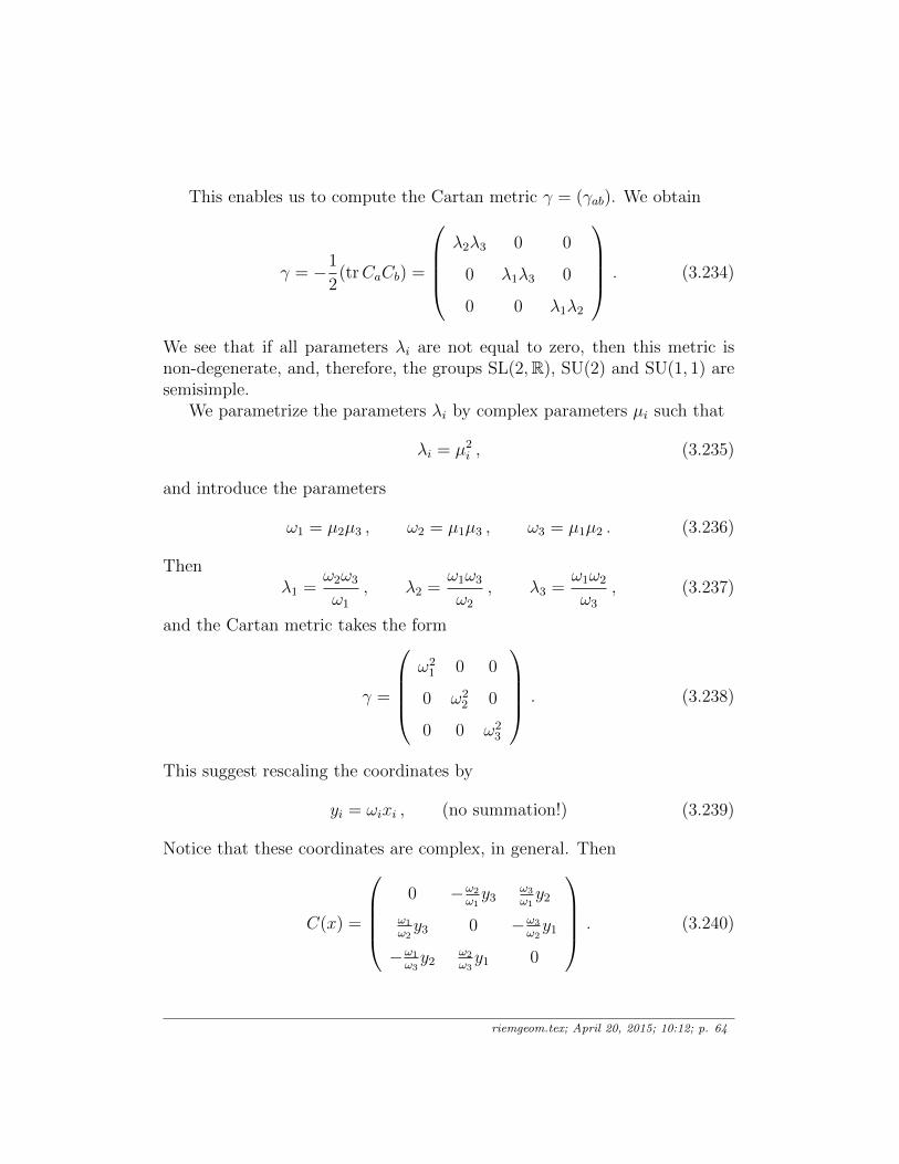
This enables us to compute the Cartan metric γ = (γab). We obtain

γ = −1

2(trCaCb) =

λ2λ3 0 0

0 λ1λ3 0

0 0 λ1λ2

. (3.234)

We see that if all parameters λi are not equal to zero, then this metric isnon-degenerate, and, therefore, the groups SL(2,R), SU(2) and SU(1, 1) aresemisimple.

We parametrize the parameters λi by complex parameters µi such that

λi = µ2i , (3.235)

and introduce the parameters

ω1 = µ2µ3 , ω2 = µ1µ3 , ω3 = µ1µ2 . (3.236)

Thenλ1 =

ω2ω3

ω1

, λ2 =ω1ω3

ω2

, λ3 =ω1ω2

ω3

, (3.237)

and the Cartan metric takes the form

γ =

ω21 0 0

0 ω22 0

0 0 ω23

. (3.238)

This suggest rescaling the coordinates by

yi = ωixi , (no summation!) (3.239)

Notice that these coordinates are complex, in general. Then

C(x) =

0 −ω2

ω1y3

ω3

ω1y2

ω1

ω2y3 0 −ω3

ω2y1

−ω1

ω3y2

ω2

ω3y1 0

. (3.240)


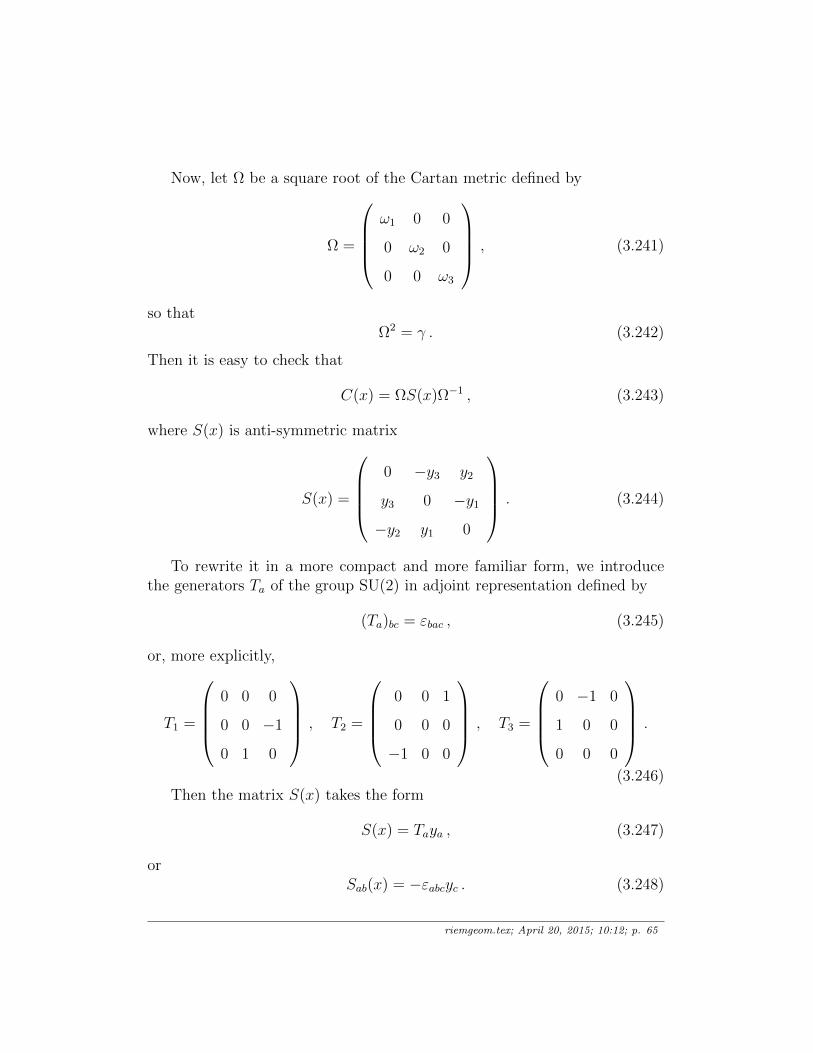
Now, let Ω be a square root of the Cartan metric defined by

Ω =

ω1 0 0

0 ω2 0

0 0 ω3

, (3.241)

so thatΩ2 = γ . (3.242)

Then it is easy to check that

C(x) = ΩS(x)Ω−1 , (3.243)

where S(x) is anti-symmetric matrix

S(x) =

0 −y3 y2

y3 0 −y1−y2 y1 0

. (3.244)

To rewrite it in a more compact and more familiar form, we introducethe generators Ta of the group SU(2) in adjoint representation defined by

(Ta)bc = εbac , (3.245)

or, more explicitly,

T1 =

0 0 0

0 0 −1

0 1 0

, T2 =

0 0 1

0 0 0

−1 0 0

, T3 =

0 −1 0

1 0 0

0 0 0

.

(3.246)Then the matrix S(x) takes the form

S(x) = Taya , (3.247)

orSab(x) = −εabcyc . (3.248)


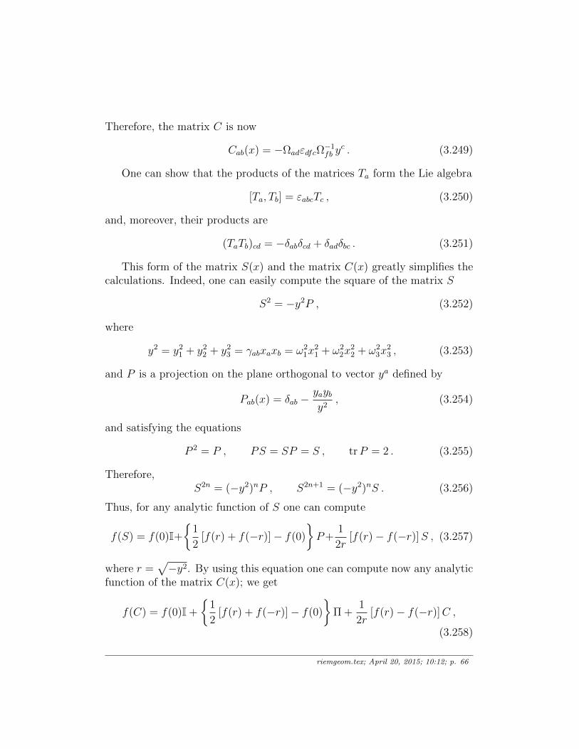
Therefore, the matrix C is now

Cab(x) = −ΩadεdfcΩ−1fb y

c . (3.249)

One can show that the products of the matrices Ta form the Lie algebra

[Ta, Tb] = εabcTc , (3.250)

and, moreover, their products are

(TaTb)cd = −δabδcd + δadδbc . (3.251)

This form of the matrix S(x) and the matrix C(x) greatly simplifies thecalculations. Indeed, one can easily compute the square of the matrix S

S2 = −y2P , (3.252)

where

y2 = y21 + y22 + y23 = γabxaxb = ω21x

21 + ω2

2x22 + ω2

3x23 , (3.253)

and P is a projection on the plane orthogonal to vector ya defined by

Pab(x) = δab −yayby2

, (3.254)

and satisfying the equations

P 2 = P , PS = SP = S , trP = 2 . (3.255)

Therefore,S2n = (−y2)nP , S2n+1 = (−y2)nS . (3.256)

Thus, for any analytic function of S one can compute

f(S) = f(0)I+

1

2[f(r) + f(−r)]− f(0)

P+

1

2r[f(r)− f(−r)]S , (3.257)

where r =√−y2. By using this equation one can compute now any analytic

function of the matrix C(x); we get

f(C) = f(0)I +

1

2[f(r) + f(−r)]− f(0)

Π +

1

2r[f(r)− f(−r)]C ,

(3.258)


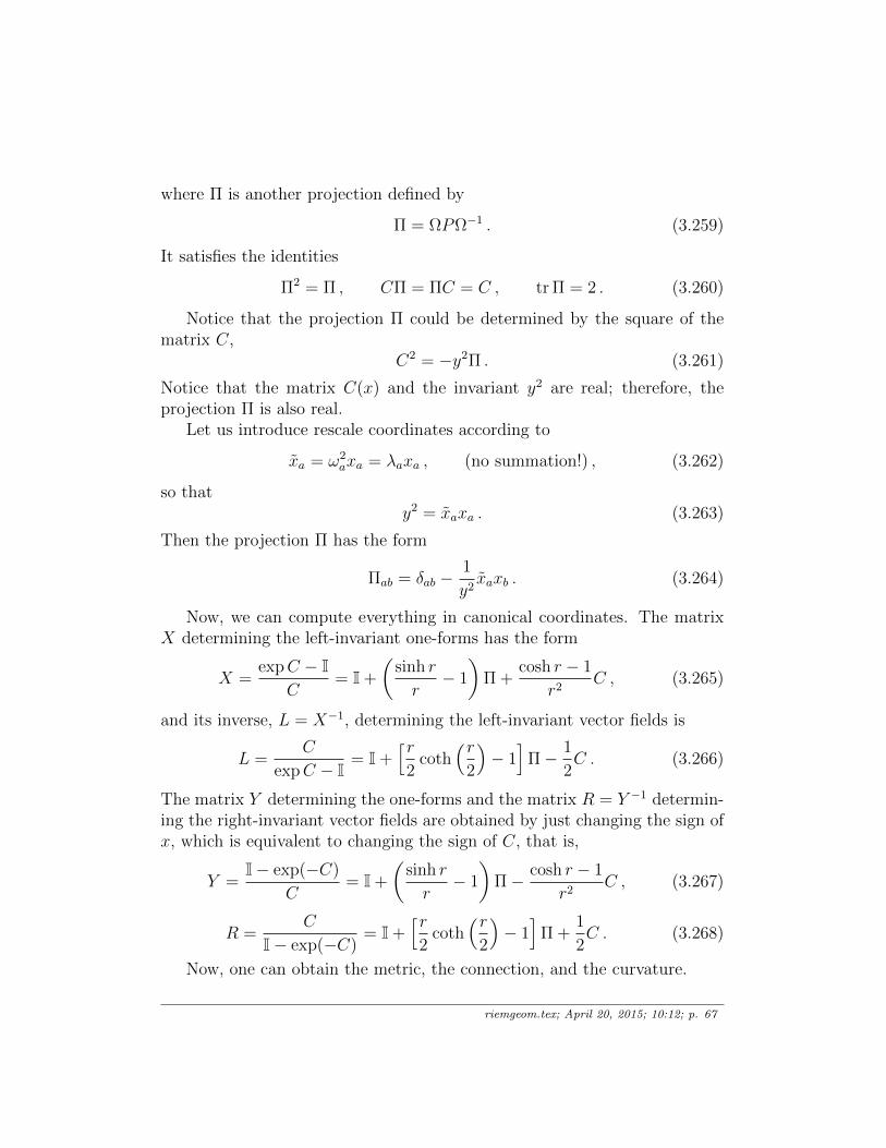
where Π is another projection defined by

Π = ΩPΩ−1 . (3.259)

It satisfies the identities

Π2 = Π , CΠ = ΠC = C , tr Π = 2 . (3.260)

Notice that the projection Π could be determined by the square of thematrix C,

C2 = −y2Π . (3.261)

Notice that the matrix C(x) and the invariant y2 are real; therefore, theprojection Π is also real.

Let us introduce rescale coordinates according to

xa = ω2axa = λaxa , (no summation!) , (3.262)

so thaty2 = xaxa . (3.263)

Then the projection Π has the form

Πab = δab −1

y2xaxb . (3.264)

Now, we can compute everything in canonical coordinates. The matrixX determining the left-invariant one-forms has the form

X =expC − I

C= I +

(sinh r

r− 1

)Π +

cosh r − 1

r2C , (3.265)

and its inverse, L = X−1, determining the left-invariant vector fields is

L =C

expC − I= I +

[r2

coth(r

2

)− 1]

Π− 1

2C . (3.266)

The matrix Y determining the one-forms and the matrix R = Y −1 determin-ing the right-invariant vector fields are obtained by just changing the sign ofx, which is equivalent to changing the sign of C, that is,

Y =I− exp(−C)

C= I +

(sinh r

r− 1

)Π− cosh r − 1

r2C , (3.267)

R =C

I− exp(−C)= I +

[r2

coth(r

2

)− 1]

Π +1

2C . (3.268)

Now, one can obtain the metric, the connection, and the curvature.


3.13 Example: SO(n)

Let us consider a specific example of a compact simple group SO(4). TheBetti numbers for this group are

B0 = B6 = 1 , B3 = 2 . (3.269)

The algebra of this group consists of real 4 × 4 traceless anti-symmetricmatrices and the dimension of this groups is dim SO(4) = 6. We considerthe group SO(n) for generality and will specify n = 6 later. The generatorsof this algebra Tij can be labeled by two indices, ij such that i, j = 1, . . . , nand i < j. The Lie algebra has the form

[T ij, Tkl] = −4δ[i[kTj]l] , (3.270)

which can be written in the form

[Tij, Tkl] =1

2Crs

ij,klTrs . (3.271)

where the structure constants are

Crsij,kl = 8δ[r [iδj][kδ

s]l] . (3.272)

The factor 12

appears because we formally sum over all indices, whereas weshould only sum over r < s. Such factors will appear elsewhere too. TheCartan metric defined by

(α, β) =1

4γij,klα

ijβkl , (3.273)

has the form

γij,kl = −1

4Crs

ij,pqCpqkl,rs (3.274)

which can be computed now easily

γijkl = 16(n− 2)δ[i[kδj]l] . (3.275)

This defines a positive definite quadratic form (for n > 2)

(α, β) =1

4γij,klα

ijβkl = 4(n− 2)αijβij . (3.276)


Notice thatδ[i[kδ

j]l]δ

[k[rδ

l]s] = δ[i[rδ

j]s] (3.277)

therefore, the tensor 2δ[i[kδj]l] plays the role of the identity in the sense that

1

2

(2δ[i[kδ

j]l]

) (2δ[k [rδ

l]s]

)= 2δ[i[rδ

j]s] . (3.278)

Therefore, the inverse of this metric, which will be denoted by γijkl, shouldbe defined so that

1

2γij,rsγrs,kl = 2δ[i[kδ

j]l] , (3.279)

it reads

γijkl =1

4(n− 2)δ[i[kδ

j]l] . (3.280)

Thus, this group is semi-simple (for n > 2) and has a bi-invariant metric.The curvature of this metric is

Rij,kl,rs,pq =1

16γab,cdC

abij,klC

cdrs,pq . (3.281)

This can be computed now; we obtain

Rij,kl,rs,pq = 32(n− 2)δ[i[rδ

j][kδ

[ql]δ

p]s] − δ[i[qδj][kδ[rl]δs]p]

. (3.282)

Here the position of indices on the right-hand side should not mean anything;it is just written in this way for readability (they all should be down indices).Also, there is anti-symmetrization over pairs of the pairs of indices ij, kl, rsand pq separately. The Ricci tensor is

Rij,rs =1

64γkl,pqγab,cdC

abij,klC

cdrs,pq . (3.283)

We compute

Rij,rs =(n− 2)

16δ[i[rδ

j]s] , (3.284)

which should be equal to 14γij,rs.

Now, for any vector X ij on the group we have

Ric(X,X) =1

4Rij,rsX

ijXrs =(n− 2)

64XijX

ij . (3.285)

This is strictly positive for any non-zero X. Also, for any two-form (or ananti-symmetric tensor X ij,kl, that is, X ij,kl = −Xkl,ij) we have

Riem(X,X) =1

64Rij,kl,rs,pqX

ij,klXrs,pq = (n− 2)X ijjlXip

pl . (3.286)

This is also strictly positive for any non-zero X.


3.14 Particular case: SO(4)


References


Riemannian Geometry, Lie Groups and Geometric...

Documents

Transcript of Riemannian Geometry, Lie Groups and Geometric...

References

riemgeom.tex; April 20, 2015; 10:12; p. 71
![Sub-Riemannian geometry, Hamiltonian dynamics, micro ... · Sub-Riemannian (SR) geometry in the framework of geometric optimal control was rst explored in the seminal article [17].](https://static.fdocuments.in/doc/165x107/5f4e7dcbb6f9633f2c3be174/sub-riemannian-geometry-hamiltonian-dynamics-micro-sub-riemannian-sr-geometry.jpg)