RI&DSH7RZQ - COnnecting REpositories · The creation of automated ﬂuid effects for ﬁlm and...

Univers

ity of

Cap

e Tow

n

The copyright of this thesis vests in the author. No quotation from it or information derived from it is to be published without full acknowledgement of the source. The thesis is to be used for private study or non-commercial research purposes only.

Published by the University of Cape Town (UCT) in terms of the non-exclusive license granted to UCT by the author.

Univers

ity of

Cap

e Tow

n

Parallel fluid dynamics for the film andanimation industries

A DISSERTATIONSUBMITTED TO THE DEPARTMENT OF COMPUTER SCIENCE,

FACULTY OF SCIENCEAT THE UNIVERSITY OF CAPE TOWN

IN FULFILLMENT OF THE REQUIREMENTSFOR THE DEGREE OFMASTER OF SCIENCE

By Ashley Reid1

Supervised by: James Gain2and Michelle Kuttel3

Submitted on 18th May 2009

[email protected]@[email protected]

Univers

ity of

Cap

e Tow

n

Abstract

The creation of automated fluid effects for film and media using computer simulations is popular, as artist timeis reduced and greater realism can be achieved through the use of numerical simulation of physical equations.The fluid effects in today’s films and animations have large scenes with high detail requirements. With theserequirements, the time taken by such automated approaches is large. To solve this, cluster environmentsmaking use of hundreds or more CPUs have been used. This overcomes the processing power and memorylimitations of a single computer and allows very large scenes to be created. One of the newer methods forfluid simulation is the Lattice Boltzmann Method (LBM). This is a cellular automata type of algorithm, whichparallelizes easily. An important part of the process of parallelization is load balancing; the distribution of com-putation amongst the available computing resources in the cluster. To date, the parallelization of the LatticeBoltzmann method only makes use of static load balancing. Instead, it is possible to make use of dynamic loadbalancing, which adjusts the computation distribution as the simulation progresses.

Here, we investigate the use of the LBM in conjunction with a Volume of Fluid (VOF) surface representation ina parallel environment with the aim of producing large scale scenes for the film and animation industries. TheVOF method tracks mass exchange between cells of the LBM. In particular, we implement the new dynamicload balancing algorithm to improve the efficiency of the fluid simulation using this method. Fluid scenes fromfilms and animations have two important requirements: the amount of detail and the spatial resolution of thefluid. These aspects of the VOF LBM are explored by considering the time for scene creation using a singleand multi-CPU implementation of the method. The scalability of the method is studied by plotting the runtime, speedup and efficiency of scene creation against the number of CPUs. From such plots, an estimate isobtained of the feasibility of creating scenes of a giving level of detail. Such estimates enable the recommen-dation of architectures for creation of specific scenes.

Using a parallel implementation of the VOF LBM method we successfully create large scenes with great detail.In general, considering the significant amounts of communication required for the parallel method, it is shownto scale well, favouring scenes with greater detail. The scalability studies show that the new dynamic loadbalancing algorithm improves the efficiency of the parallel implementation, but only when using lower numberof CPUs. In fact, for larger number of CPUs, the dynamic algorithm reduces the efficiency. We hypothesisethe latter effect can be removed by making using of centralized load balancing decision instead of the currentdecentralized approach. The use of a cluster comprising of 200 CPUs is recommended for the production oflarge scenes of a grid size 6003 in a reasonable time frame.

1

Univers

ity of

Cap

e Tow

n

Acknowledgments

In the end, this was a difficult Masters. I discovered that writing is hard, more precisely, being exact with thesethings called “words” is hard. I would like to thank my supervisors, James Gain and Michelle Kuttel, for helpingwith this particular endeavor and of course the rest of the effort that they put into the work resulting in thisdocument. Thank you to Duncan Clough for his proof reading.

Life and this thesis would be pointless if it were not for the people around me. I would like to thank my parents,Graham and Shez, for their tireless efforts in providing for me and putting up with my comings and goings. Thegroup that was particularly supportive in the mad days before I left for Germany: Fritz (for late night DOTA),Kath (for boundless energy), Mary (for late night work parties), Ingrid (for always smiling), Duncs (for all thepolitics and exercise), Neil (for the chats over coffee and Chinese), Melch (for the guitar) and Lindsay (for thepositivity). To various friends who supported me during this task: Sally-Anne (for energy and ’life’ support),Kers (for big sister type advice) and Jan (for squash and perspective).

The people on campus: Thyla (for much tea/coffee and philsophical discussion, in truth I owe greater grat-itude for the Maths degree), Chris de Kadt for always speaking his mind, causing trouble and not acceptingsecond rate thought), Carl (for the NVIDIA leg up and all the work into UCT computer science), Andrew (formany laughs and always improving our lives as students), Dave (for joining forces for our publication and ofcourse for gyming), Ian (for being taller than me and for the braai’s), Jannie (for the expert DOTA technique)and Bertus (for still being there).

I would to thank the Centre for High Performance Computing in Cape Town for the use of their machines,they filled a great need and without that the thesis would have been delayed much longer. They have awonderful attitude towards developing research in South Africa. In particular, I would like to thank SebastianWyngaard for his help in setting up this connection.

I would like to thank NVIDIA for the donation of the graphics cards to the lab, which aided in the develop-ment process, and for their involvement at UCT. They have given me and many the opportunity of overseasexposure and extra funding through internships.

With hesitancy, I thank God for creating a world that is very complex. I still haven’t decided if this is a goodthing or not. Hopefully, this thesis explains a part of it correctly.

2

Univers

ity of

Cap

e Tow

n

Notation

Here, we give brief definitions of the symbols used in the derivations and proofs. The definitions are given inthree dimensions, but are similarly defined in two dimensions.

Scalars, Vectors and functions

Vectors are given using the arrow notation and scalars without. For example, the scalar pressure is be writ-ten as P and the velocity is −→u = (ux, uyuz), with co-ordinates of velocity given by ux,uy and uz. The vector−→x = (x, y, z) is used to represent the position vector in three dimensions.

Functions may map to a scalar value or a vector value. In the previous example, P may be a function ofposition, x, y and z. This is denoted as P (x, y, z), or P (−→x ) in short form. An example of a vector valued func-tion is the velocity at any point in space, −→u (−→x ) = (f(−→x ), g(−→x ), h(−→x )), where f, g and h are functions mappingfrom R3 → R. Often, the inputs to a function will not be included, i.e.−→u (−→x ) is written simply as −→u .

Partial Derivatives

∂f∂x denotes the partial derivative of f with respect to x, where f is a scalar valued function. This is obtained byassuming f to be constant with respect to all other variables besides x.

The gradient of a scalar function is given by

∇f =

(∂f

∂x,∂f

∂y,∂f

∂z

)=

∂f

∂−→x.

Again, for scalar f , the divergence operator is

∇ · f =∂f

∂x+∂f

∂y+∂f

∂z.

Now, ∂−→u∂x for a vector valued function is calculated co-ordinate wise, ∂−→u

∂x =(∂f∂x ,

∂h∂x ,

∂g∂x

). The gradient of a

vector function is called the Jacobian and is defined as

3

Univers

ity of

Cap

e Tow

n

4

∇−→u = ∇(f, g, h) =

∂f∂x

∂h∂x

∂g∂x

∂f∂y

∂h∂y

∂g∂y

∂f∂z

∂h∂z

∂g∂z

.

The Laplacian is given as

∇2−→u =∂2−→u∂2x

+∂2−→u∂y2

+∂2−→u∂z2

.

And, finally, the curl of the velocity field, −→u , is

∇×−→u =

(∂w

∂y− ∂v

∂z,∂u

∂z− ∂w

∂x,∂v

∂x− ∂u

∂y

).

Tensors

The tensor notation, uαuβ , is used on occasion to indicate the sum of all combinations of co-ordinates of −→u ,i.e. α, β = 1, 2, 3.

The delta function, δαβ , is the indicator function, equal to 1 if α = β and 0 otherwise

Univers

ity of

Cap

e Tow

n

Contents

1 Introduction 12

1.1 Motivation . . . . . . . . . . . . . . . . . . . . . . . . . . . . . . . . . . . . . . . . . . . . . . . . . 13

1.2 Aims and Evaluation . . . . . . . . . . . . . . . . . . . . . . . . . . . . . . . . . . . . . . . . . . . 14

1.3 Contributions and results . . . . . . . . . . . . . . . . . . . . . . . . . . . . . . . . . . . . . . . . 16

1.4 Thesis Structure . . . . . . . . . . . . . . . . . . . . . . . . . . . . . . . . . . . . . . . . . . . . . 17

2 Background 18

2.1 Computer Simulation . . . . . . . . . . . . . . . . . . . . . . . . . . . . . . . . . . . . . . . . . . . 18

2.2 Fluid Simulation . . . . . . . . . . . . . . . . . . . . . . . . . . . . . . . . . . . . . . . . . . . . . 20

2.3 First Approaches and the Navier-Stokes Equations . . . . . . . . . . . . . . . . . . . . . . . . . . 21

2.4 Simulation Methods . . . . . . . . . . . . . . . . . . . . . . . . . . . . . . . . . . . . . . . . . . . 23

2.5 The Fluid Surface . . . . . . . . . . . . . . . . . . . . . . . . . . . . . . . . . . . . . . . . . . . . . 31

2.6 Parallel Programming . . . . . . . . . . . . . . . . . . . . . . . . . . . . . . . . . . . . . . . . . . 33

2.7 Using High Performance Computing . . . . . . . . . . . . . . . . . . . . . . . . . . . . . . . . . . 37

2.8 Conclusion . . . . . . . . . . . . . . . . . . . . . . . . . . . . . . . . . . . . . . . . . . . . . . . . 38

3 LBM Fluid Simulation 40

3.1 Full Algorithm Description for 3D . . . . . . . . . . . . . . . . . . . . . . . . . . . . . . . . . . . . 40

3.2 Physical Derivation . . . . . . . . . . . . . . . . . . . . . . . . . . . . . . . . . . . . . . . . . . . . 44

3.3 Conclusion . . . . . . . . . . . . . . . . . . . . . . . . . . . . . . . . . . . . . . . . . . . . . . . . 51

4 Single CPU Implementation 52

4.1 Algorithm Summary . . . . . . . . . . . . . . . . . . . . . . . . . . . . . . . . . . . . . . . . . . . 52

4.2 Volume of Fluid Method . . . . . . . . . . . . . . . . . . . . . . . . . . . . . . . . . . . . . . . . . 53

5

Univers

ity of

Cap

e Tow

n

CONTENTS 6

4.3 Fluid Surface Generation . . . . . . . . . . . . . . . . . . . . . . . . . . . . . . . . . . . . . . . . 56

4.4 Houdini Integration . . . . . . . . . . . . . . . . . . . . . . . . . . . . . . . . . . . . . . . . . . . . 58

4.5 Animation Results . . . . . . . . . . . . . . . . . . . . . . . . . . . . . . . . . . . . . . . . . . . . 63

4.6 Conclusion . . . . . . . . . . . . . . . . . . . . . . . . . . . . . . . . . . . . . . . . . . . . . . . . 74

5 Parallelization 75

5.1 Introduction . . . . . . . . . . . . . . . . . . . . . . . . . . . . . . . . . . . . . . . . . . . . . . . . 75

5.2 Design . . . . . . . . . . . . . . . . . . . . . . . . . . . . . . . . . . . . . . . . . . . . . . . . . . . 76

5.3 Implementation . . . . . . . . . . . . . . . . . . . . . . . . . . . . . . . . . . . . . . . . . . . . . . 80

5.4 Conclusion . . . . . . . . . . . . . . . . . . . . . . . . . . . . . . . . . . . . . . . . . . . . . . . . 88

6 Evaluation 90

6.1 Method . . . . . . . . . . . . . . . . . . . . . . . . . . . . . . . . . . . . . . . . . . . . . . . . . . 90

6.2 Results . . . . . . . . . . . . . . . . . . . . . . . . . . . . . . . . . . . . . . . . . . . . . . . . . . 94

6.3 Conclusion . . . . . . . . . . . . . . . . . . . . . . . . . . . . . . . . . . . . . . . . . . . . . . . . 113

7 Discussion 116

7.1 Implementation and development . . . . . . . . . . . . . . . . . . . . . . . . . . . . . . . . . . . . 116

7.2 Animation Creation . . . . . . . . . . . . . . . . . . . . . . . . . . . . . . . . . . . . . . . . . . . . 117

7.3 Dynamic Load balancing parameters . . . . . . . . . . . . . . . . . . . . . . . . . . . . . . . . . . 119

7.4 Scalability and Efficiency . . . . . . . . . . . . . . . . . . . . . . . . . . . . . . . . . . . . . . . . 119

7.5 Architecture and scene scale recommendations . . . . . . . . . . . . . . . . . . . . . . . . . . . 121

8 Conclusions 123

8.1 Thesis Aims . . . . . . . . . . . . . . . . . . . . . . . . . . . . . . . . . . . . . . . . . . . . . . . . 123

8.2 Recommendations and Future work . . . . . . . . . . . . . . . . . . . . . . . . . . . . . . . . . . 124

A Advanced Fluid Effects 126

B Proof of physical correctness 128

C Single CPU Profiles 133

C.1 TAU profile . . . . . . . . . . . . . . . . . . . . . . . . . . . . . . . . . . . . . . . . . . . . . . . . 133

C.2 Operation Counts . . . . . . . . . . . . . . . . . . . . . . . . . . . . . . . . . . . . . . . . . . . . . 134

Univers

ity of

Cap

e Tow

n

CONTENTS 7

D Extended Tests and Results 135

D.1 Latency and bandwidth values for CRUNCH and CHPC . . . . . . . . . . . . . . . . . . . . . . . 135

D.2 Simulations times . . . . . . . . . . . . . . . . . . . . . . . . . . . . . . . . . . . . . . . . . . . . . 139

Univers

ity of

Cap

e Tow

n

List of Figures

2.1 Two triangulations of a 2D sphere. (a) low resolution (b) high resolution. . . . . . . . . . . . . . . 19

2.2 The Marker-And-Cell (MAC) grid and the markers used in the 2D MAC grid method. . . . . . . . 23

2.3 The HPP lattice . . . . . . . . . . . . . . . . . . . . . . . . . . . . . . . . . . . . . . . . . . . . . . 27

2.4 Fluid simulated using Smoothed Particle Hydrodynamics (SPH). . . . . . . . . . . . . . . . . . . 30

2.5 Irregular domain decomposition. . . . . . . . . . . . . . . . . . . . . . . . . . . . . . . . . . . . . 36

3.1 The 3D lattice that we use is commonly known as the D3D19 lattice. . . . . . . . . . . . . . . . . 41

3.2 Distribution functions and obstacles. . . . . . . . . . . . . . . . . . . . . . . . . . . . . . . . . . . 42

3.3 The 2D lattice. . . . . . . . . . . . . . . . . . . . . . . . . . . . . . . . . . . . . . . . . . . . . . . 48

4.1 (left) The Volume of Fluid (VOF) LBM algorithm steps. (right) Scene cell division. . . . . . . . . . 53

4.2 The marching cubes algorithm illustrated. . . . . . . . . . . . . . . . . . . . . . . . . . . . . . . . 57

4.3 The Interpolated Vertices (IVs) structure used to optimise the marching cubes algorithm. . . . . . 58

4.4 Pseudocode for the marching cubes algorithm used to generate the fluid surface from the VOFfill fractions. . . . . . . . . . . . . . . . . . . . . . . . . . . . . . . . . . . . . . . . . . . . . . . . 59

4.5 The basic Houdini interface. . . . . . . . . . . . . . . . . . . . . . . . . . . . . . . . . . . . . . . . 61

4.6 An example of the dynamic fluid network. . . . . . . . . . . . . . . . . . . . . . . . . . . . . . . . 61

4.7 The parameters pane for the VOF LBM custom operator. . . . . . . . . . . . . . . . . . . . . . . 62

4.8 The falling drop at different spatial resolutions (∆t = 0.05s, S = 0.03 and G = 50× 50× 50). . . 65

4.9 The falling drop for different Smagorinsky constants (∆t = 0.01s, ∆x = 0.0004 and G = 50 ×50× 50). . . . . . . . . . . . . . . . . . . . . . . . . . . . . . . . . . . . . . . . . . . . . . . . . . . 66

4.10 The falling drop for different time steps (∆x = 0.0004m, S = 0.03 and G = 50× 50× 50). . . . . . 67

4.11 The falling drop for different grid resolutions (v = 0.00001ms−1 and S = 0.03). . . . . . . . . . . . 68

4.12 The falling drop for different viscosities (∆t = 0.05s, ∆x = 0.0004m, S = 0.03 andG = 50×50×50). 69

8

Univers

ity of

Cap

e Tow

n

LIST OF FIGURES 9

4.13 Artifacts due to the grid representation at a resolution of 80x100x80. . . . . . . . . . . . . . . . . 70

4.14 The time taken to produce the 3.6s falling drop animation for different resolutions. . . . . . . . . . 71

4.15 Percentage of time spent in each of the steps during a simulation. . . . . . . . . . . . . . . . . . 71

4.16 Still pond test case. . . . . . . . . . . . . . . . . . . . . . . . . . . . . . . . . . . . . . . . . . . . 72

4.17 A analysis of the operations per cell in the stream and collide steps for the pond test case. . . . . 72

4.18 Memory usage of the VOF LBM implementation. . . . . . . . . . . . . . . . . . . . . . . . . . . . 73

5.1 Domain decomposition methods. . . . . . . . . . . . . . . . . . . . . . . . . . . . . . . . . . . . 77

5.2 The 2D domain decomposition viewed from the top. . . . . . . . . . . . . . . . . . . . . . . . . . 79

5.3 Dependent and independent cells. . . . . . . . . . . . . . . . . . . . . . . . . . . . . . . . . . . . 80

5.4 Simulation steps and required quantities. . . . . . . . . . . . . . . . . . . . . . . . . . . . . . . . 82

5.5 Simulation steps and required quantities with synchronisation. . . . . . . . . . . . . . . . . . . . 83

5.6 Flow diagram for each slave process. . . . . . . . . . . . . . . . . . . . . . . . . . . . . . . . . . 85

6.1 The five tests cases used to evaluate the parallel VOF LBM implementation. . . . . . . . . . . . . 91

6.2 The final rendered version of the water fall scene. . . . . . . . . . . . . . . . . . . . . . . . . . . . 95

6.3 The final rendered version of the water drop falling into a pool. . . . . . . . . . . . . . . . . . . . 96

6.4 The final rendered version of the shower scene, with fluid rendered as mud. . . . . . . . . . . . . 97

6.5 The final rendered version of the wave breaking over the city. . . . . . . . . . . . . . . . . . . . . 98

6.6 The final rendered version of the breaking dam. . . . . . . . . . . . . . . . . . . . . . . . . . . . . 99

6.7 Dam simulation for different parameter values on CRUNCH. . . . . . . . . . . . . . . . . . . . . . 101

6.8 Drop simulation for different parameter values. . . . . . . . . . . . . . . . . . . . . . . . . . . . . 102

6.9 The run-time for the drop and dam simulations for different computation thresholds. . . . . . . . . 102

6.10 Speedup results for all test cases. . . . . . . . . . . . . . . . . . . . . . . . . . . . . . . . . . . . 104

6.11 Efficiency results for low simulation resolutions. . . . . . . . . . . . . . . . . . . . . . . . . . . . . 105

6.12 The speedup results for the test cases at a medium resolution.. . . . . . . . . . . . . . . . . . . . 107

6.13 The efficiency results for the test cases at a medium resolution. . . . . . . . . . . . . . . . . . . . 108

6.14 The speedup results for the tests cases at high resolutions. . . . . . . . . . . . . . . . . . . . . . 110

6.15 The efficiency results for test cases at high resolutions. . . . . . . . . . . . . . . . . . . . . . . . 111

6.16 Maximum and Mean Geometric deviation for the Gnomon in mud simulation. . . . . . . . . . . . 112

Univers

ity of

Cap

e Tow

n

LIST OF FIGURES 10

6.17 Maximum Geometric deviation for static load balancing, represented by a rainbow colour scalefrom blue to red projected onto the single CPU model. . . . . . . . . . . . . . . . . . . . . . . . . 112

6.18 Profiling of simulations at low resolutions. . . . . . . . . . . . . . . . . . . . . . . . . . . . . . . . 114

6.19 Profiling of drop and dam simulations at medium resolutions. . . . . . . . . . . . . . . . . . . . . 115

C.1 A profile of the single CPU implementation. . . . . . . . . . . . . . . . . . . . . . . . . . . . . . . 133

D.1 The Pingpong_send_recv times using SKaMPI. . . . . . . . . . . . . . . . . . . . . . . . . . . . . 136

D.2 Wallclock time for simulations on the CHPC and CRUNCH architectures. . . . . . . . . . . . . . . 137

D.3 Speedup and efficiency results for dam for a grid resolution of 100× 100× 100. . . . . . . . . . . 138

D.4 Speedup and efficiency results for dam for a grid resolution of 100× 100× 100. . . . . . . . . . . 138

D.5 Wall clock time for simulations at medium resolutions . . . . . . . . . . . . . . . . . . . . . . . . 139

D.6 Wall clock time for simulations at medium resolutions . . . . . . . . . . . . . . . . . . . . . . . . 140

D.7 Wall clock time for simulations at high resolutions . . . . . . . . . . . . . . . . . . . . . . . . . . 141

Univers

ity of

Cap

e Tow

n

List of Tables

4.1 Modified mass exchanges to reduce lone interface cells. . . . . . . . . . . . . . . . . . . . . . . . 56

4.2 The space taken up by one cell in the VOF LBM implementation. . . . . . . . . . . . . . . . . . . 71

5.1 The two different clusters on which we ran our simulations. . . . . . . . . . . . . . . . . . . . . . 87

6.1 The tests that will be run to determine the scalability of the system. . . . . . . . . . . . . . . . . . 93

A.1 An overview of the advanced fluid methods that have been researched by different authors. . . . 127

C.1 The operations used during the stream and collide steps of the LBM for the still pond test case. . 134

11

Univers

ity of

Cap

e Tow

n

Chapter 1

Introduction

Directors seek to produce films or advertisements with complex fluid effects that add realism to scenes and,ultimately, a more visually pleasing experience to viewers. Due to the large scale and fantastical nature ofmany of the scenes required for competitive visual effects, there has been a significant body of research intocreating fluid using computer simulations. These methods have been helped by the increase in CPU powerand parallel systems that use architectures such as clusters. The end result is effective fluid simulation for thefilm and animation industries.

Computer simulations use many methods to approximate fluid, often making use of physical equations todescribe fluid behaviour. Algorithms are then created using these equations to produce fluid effects. The fluidis used as it is or is used together with other visual elements, such as adding water to a city filmed from above.One of the newer and less tested algorithms for fluid simulation is the Lattice Boltzmann method. This thesisadds to the research on the Lattice Boltzmann Method (LBM) by analysing the algorithm and the parallel imple-mentation thereof, to see what scale of fluid effects can be created with different computing resources. Broadlyspeaking, the simulation scale is measured by the detail of the final product, but this will be more rigorouslydefined in the testing section of the thesis.

The LBM is a cellular automata method that simulates fluid movement using a grid and sets of particle dis-tribution functions. The distribution functions represent the movement of molecules within the fluid. Fluid issimulated by stepping these distribution functions through time using update rules. The rules are based onphysical equations that predict the movement of fluid molecules that are moving and colliding.

There are many types of fluids and they can be classified into two groups: liquids or gases. The definingdifference is that a liquid has a definite surface that can freely move, called the free-surface. This gives theportion of space that is occupied by the fluid. For the LBM, a Volume of Fluid (VOF) method uses the simulationof the underlying fluid interactions to track a free-surface.

In our context, computing resources range from a single Dual Core desktop to over a thousand computersin a cluster environment. These resources must be used as efficiently as possible and the LBM implementa-tion must optimise the use of the resources by dividing the fluid simulation up between the cores or CPUs inthe best possible way. This process is known as load balancing. Currently, there are only more straightforwardparallel implementations that make use of static load balancing. In this case, the simulation is divided up once,

12

Univers

ity of

Cap

e Tow

n

CHAPTER 1. INTRODUCTION 13

at the beginning. We implement this method of load balancing and a new dynamic method, that allows theshifting of the simulation division as time progresses.

These implementations are tested to calculate the length of time to simulate a scene with a given level ofdetail. In conjunction with tests of a single CPU LBM implementation, the efficiency of each of the algorithmscan thus be measured. Once the efficiency of the implementations has been determined, recommendationscan be made about the computing resources required to achieve a suitable level of detail within a given timeframe. This is important for media producers, as they need fast turn around times during production and goodestimates will tell us if the LBM is suitable for the media industry.

The next section provides a motivation for this thesis. The evaluation criteria and testing outline is in Sec-tion 1.2, while section 1.3 outlines the main contributions and results. The last section contains an overview ofthe thesis structure.

1.1 Motivation

Visual effects are widespread in today’s media, particularly in films and advertisements. These effects enhancemedia and make them more entertaining for viewers. Some examples of scenes making use of visual effectsinclude: sinking ships, exploding objects and non-existent characters created with computer graphics (CG).High quality visual effects are important, as they make the viewer feel immersed. Such effects are difficult tocreate by conventional means, either because the scenes required are not easily created in real life or becausethe costs are prohibitive. Sometimes the effects are added onto real camera footage, while there are manycases where entire scenes and even entire 3D animated films, such as Shrek, are created in CG. These effectscan be created by artists, by using special camera techniques, or with computer software.

Fluids, such as water, are found in many scenes. They are the cause of some of the most impressive andcomplex natural effects seen in everyday life. Take the examples of a ship sinking or an object exploding.Media producers seek to recreate fluid effects, but scenes such as a city being swamped with water are notpractically possible. It is very important to capture fluid behaviour correctly, as it is well defined by physicalequations and viewers can easily tell when water is behaving incorrectly. In fully CG Media, all fluids haveto be recreated, including honey, oil and air. The last is a particularly interesting case. Although it is notvisible to the human eye, air can be treated as a fluid and its effects, such as wind, influence scene objects.Although the different types of fluid are related, the focus of this thesis will be on the class of fluids called liquids.

Simulation methods are a means of recreating real world behaviours without needing all the real world ele-ments present. In the case of fluids, the individual molecules that make up the fluid are ignored. One meansof simulating fluids is by creating down-scaled versions of the scene, for example, by filming a much smalleramount of water flooding a model of a city that is to be swamped. This gives a somewhat similar result to whatwould be seen for the full size city, but the different scale is often apparent in the final shot. These separatelyfilmed shots can either be used as they are, or overlayed with other footage to provide the final shot, a processknown as compositing. The fluid effects can also be drawn in two dimensions and overlayed onto the finalimage, but this requires an artist to draw the fluid for every frame. These two approaches do not use physicalequations to govern the behaviour of fluids.

Univers

ity of

Cap

e Tow

n


Fluid behaviour is caused by the molecular forces between millions, or even billions, of molecules makingup the fluid. Due to the number of atoms and overall force complexity, simulating all the atoms and the forcesis currently computationally not feasible [Stam, 1999]. Instead, approximate simulations are used to augmentcurrent scenes with visual fluid effects. The simulations often use low detail approximations or do not give thecorrect fluid behaviour due to the use of simplified physical equations [Foster and Metaxas, 1997]. Again, thefluid shots generated from the computer simulations are used as they are or are combined with other real worldcamera shots, with possible alteration by artists.

A more ideal approach is to fully simulate the fluid in 3D as closely as possible without input from the artist.This approach has become increasingly popular, as it provides the most realistic behaviour with the least inputeffort. This lowers the cost of producing a scene. Additionally, in a 3D scene it is not always possible for anartist to capture all fluid detail. Full computer simulations aim to recreate scenes with more detail than anartist would be able to achieve. Due to the faster processing power of today’s Central Processing Units (CPUs)and improved simulation algorithms the full simulation approach has become more feasible [Irving et al., 2006].

Media producers have many deadlines to meet and the time to create a scene is crucial, hence the simu-lation times need to be as fast as possible. Individual CPUs have improved vastly in their performance andparallel chips with two and four cores are commonplace. One way to speed up the simulations is through theuse of parallel algorithms, which make use of the extra cores on single CPUs and multiple CPUs, in environ-ments such as clusters. The use of such techniques can bring simulations, which previously could only runon one CPU and took days or weeks, down to a matter of minutes or hours when running on hundreds of CPUs.

Naturally, the time required for the simulation will be relative to the amount of detail that is being simulatedin the scene. For the LBM, which simulates fluids on a grid, the simulation scale is given by the simulationgrid size [Thurey, 2007]. Effectively, the larger the number of grid cells, the more individual sections of fluidare being simulated. The more individual pieces of fluid simulated, the greater the quality of the final fluidsimulation produced. Juxtaposed to this concept is the spatial resolution of the simulation, which measureshow much each individual piece of fluid represents in the real world. One grid cell could correspond to 1m3 offluid, where small droplets are not simulated, or 1cm3, where large bodies of water require large numbers ofgrid cells for accurate representation.

1.2 Aims and Evaluation

The target market is liquid animations for the film and animation industries. Both these markets require highlydetailed fluid surfaces, but unlike fluids for a gaming platform, the simulation model need not run in real-time.However, to produce a good final product, an animator will need to examine the surface generated by thefluid model and may make modifications to the scene or the model to obtain acceptable results. This placesrestrictions on the running time of simulations, as a long run time reduces turn around time during production.

The aim of this thesis is to create a system that efficiently uses many CPUs to simulate fluid for a 3D scenewithin the target market’s time frame. In particular, we investigate the scalability of the system with respect torequired fluid detail. We have developed a system that is able to produce fluids by running physical simulationusing the VOF LBM to produce fluid surfaces for a given 3D scene. We run scalability and efficiency tests, withrespect to the number of CPUs used, using this implementation.

Univers

ity of

Cap

e Tow

n


For the purposes of this thesis, three VOF LBM implementations will be created: for single CPU, for multi-CPU with static load balancing and a multi-CPU with dynamic load balancing.

The aims of this thesis are:

1. to produce large scale simulations of fluid;

2. To evaluate the robustness of the VOF LBM for simulating fluids with a free surface using a single CPUimplementation;

3. to estimate the simulation scales and spatial resolution that can be created using a single CPU imple-mentation of the VOF LBM;

4. to compare the performance and scalability, with respect to the number of CPUs, of the static and dy-namic load balancing implementations of the VOF LBM;

5. to recommend the architecture required to achieve particular simulation scales using the parallel versionof the VOF LBM.

Note, we developed two different implementations of the multi-CPU fluid simulation, one that makes use of thestatic load balancing and one with dynamic load balancing. Both will need to be evaluated with respect to theappropriate aims.

Evaluation of both the single - and multi-CPU implementations will consider whether the simulations producedare realistic, the possible range of values for the adjustable parameters and the performance (run time andmemory consumption) of the system. An analysis of the effects that are achieved using this software will beperformed. To our knowledge, a detailed analysis for the VOF LBM algorithm is not provided in literature.Firstly, it is important that the VOF LBM algorithm produces adequate fluid motion. As the target application isvisual effects, the results do not need to be physically correct, but they must look realistic and have no visuallyjarring artifacts.

As with most simulations, there are a number of different parameters that are used in the algorithm. Thedifferent possible parameter values are tested to verify the robustness of the algorithm. We try to find out ifthere are points where the algorithm breaks and in which situations it can be used.

The performance of the single CPU implementation is also important. An analysis of the run time and memoryconsumption of the single CPU implementation is provided to determine at what scale it is feasible to producefluid simulations with a single CPU.

The next part of the evaluation is concerned with the multi-CPU implementations; as these implementationsmay produce incorrect results, validation of the multi-CPU implementations is performed. We conduct a com-parison of the same simulation generated by the single CPU implementation. A simulation is consideredadequate as long as it looks realistic even if the results deviate slightly from the single CPU generated fluid.

To evaluate the performance and scalability of the two multi-CPU implementations, a number of different testscenes are constructed. These scenes are inspired by those currently required in today’s visual effects. The

Univers

ity of

Cap

e Tow

n


scenes are: a water fall scene, a wave breaking over a city (inspired from the movie The Day After Tomorrow1),Gnomon2 showering in water/mud (inspired from Shrek3), Breaking Dam (from the literature [Thürey, 2003])and water drop falling into a pool (also from literature [Pohl and Rüde, 2007]). The time taken for a completesimulation is compared against the number of CPUs used for the simulation. This provides an indication asto how efficient the VOF LBM is in a multi-CPU environment and at what level of fluid detail it is feasible toproduce simulations.

1.3 Contributions and results

We provide a scalability analysis of the parallel VOF LBM simulation that makes use of a new dynamic loadbalancing scheme. No similar study can be found in literature.

In addition, several topics have been researched to contribute to this thesis. Firstly, the new scheme needs tobe compared against the currently used static load balancing scheme and a scalability analysis of the parallelVOF LBM simulation using static load balancing is performed for this purpose.

As there is no easily accessible derivation and correctness proof for the LBM in current literature, simpleversions are developed. A distributed fluid simulation plug-in for Houdini, which uses the VOF LBM for thephysical simulation was created to allow scene specification. Houdini is a popular 3D software package cre-ated by SideFX4. It has been used in many of the latest movie titles, such as Spiderman Three, and has asingle CPU fluid simulation tool, but no distributed version.

The fluid simulation will be used by artists and, therefore, the fluid animation should be produced correctlyfor different input parameters. Hence, an analysis of the single CPU VOF LBM implementation for robustnesswith respect to input parameters has been performed. With the this and the other analyses mentioned, wemake feasibility recommendations for producing scenes of a specific detail.

The first result from this thesis is that the VOF LBM was found not to be very stable and requires extra stabilityenhancements. Due to these stability conditions, the length of a cube domain that can be simulated is of theorder of 10cm, which is far from ideal if a city flood is to be simulated. However, in practice, simulating a city atthese orders of spatial resolution, produces reasonable final animations as shown in the results section.

For low grid resolutions, of the order of 1003 (and hence low fluid detail), the parallel implementation of both thestatic and dynamic load balancing scale poorly. Higher resolutions, 3003 and greater, scale at better rates. Thedynamic load balancing only enhances the efficiency of simulations for lower numbers of CPUs and reducesthe efficiency for large numbers of CPUs. In general, there is a crossover point where the static load balancingstarts performing better then the dynamic version. The poor scaling at large CPU numbers for the dynamicsimulation was found to be caused by badly chosen load balances. The maximum run time for a individualslave process for dynamic algorithm was worse than the static algorithm. This is due to local load balancingdecisions.

1http://www.imdb.com/title/tt0319262/2A fantastical Digimon character from TV.3www.shrek.com4www.sidefx.com

Univers

ity of

Cap

e Tow

n


The cause of the poor scaling was found to be the dependency of the parallel LBM algorithm on synchro-nisation. This requires constant communication, which remains the same for all numbers of CPUs. However,considering the amount of communication required, the scaling can be considered good.

The first recommendation made is that the general stability of the algorithm is poor and the basic stabilityimplementations need to be replaced with more advanced measures. Secondly, we note that Infiniband isthe best interconnect for use in the cluster environment. From the scalability analysis’s, we conclude that theproduction a high resolution simulation at a grid size of 6003 in a reasonable time frame requires a cluster of200 CPUs. A reasonable time frame is defined relative to turn around time within a working day or week.

It is very important to establish simulation correctness and we recommend an implementation that can checkfor simulation correctness in an automated fashion. This is necessary when implementing optimisations, es-pecially in a cluster environment, as the software can quickly become large and unmanageable.

The last recommendation is that the dynamic load balancing algorithm needs to use the global computa-tion time for each slave process for better load balancing decisions. The current implementation, suffers fromsub-optimal balances due to only using local information.

1.4 Thesis Structure

The thesis is comprised of seven chapters, which are organised as follows:

• Chapter 2 discusses computer simulations. It covers how simulations are defined and the general ap-proaches to creating fluid using physical equations. The choice of the LBM is motivated.

• Chapter 3 then goes into the details of the physical equations from which the LBM is derived. Thisprovides specifics required for the implementation of the method. The stability of the method is discussed.

• Chapter 4 provides details of the implementation of single CPU version for fluid simulation. The VOF sur-face representation is introduced and the integration of the simulation into the software package Houdiniis outlined. The results of the simulation are provided to show what effects are achievable with the VOFLBM. The robustness of the method with respect to the input parameters is explored.

• The parallelization of the VOF LBM is presented in Chapter 5. Technologies for the parallelization areintroduced and the problems arising from them are discussed. To improve the efficiency of the parallelimplementation, we make use of load balancing. Both static and dynamic load balancing algorithms areoutlined.

• Chapter 6 presents the results of the parallel simulations. A number of test cases are presented. Thesystem correctness of the parallel implementation is validated against the single CPU implementation andthe optimal choice of load balancing parameters are explored. Given these parameters, the scalability ofthe simulations is analysed. Further insight into the performance of the parallel version is gained fromcomparisons of the load balancing methods and code profiling.

• Lastly, the results are discussed and conclusions drawn in Chapter 7 and 8. Recommendations are givenfor the required or preferred architectures for producing fluid simulations at a given detail level.

Univers

ity of

Cap

e Tow

n

Chapter 2

Background

There has been considerable research in the field of fluid simulation across many different disciplines, such asengineering, physics and computer graphics. The first two fields naturally seek methods that produce physi-cally correct behaviour and the last, something that is visually convincing. This chapter introduces computersimulations and fluid concepts. Early approaches to fluid simulation are discussed, with an emphasis on themost popular methods and their application in computer graphics. In addition, we provide motivation for thechoice of the Lattice Boltzmann Method for fluid simulation over other approaches and explain why the par-allelization of fluid simulations is an interesting problem worth investigating. As advanced fluid effects arenot within the scope of the thesis, such background information has been excluded from this chapter. Theinterested reader is referred to Appendix A for a summary of effects currently researched.

2.1 Computer Simulation

It is desirable to use computers to simulate the real world, as they can perform millions of calculations persecond without supervision. However, to do this, real world objects need to be represented appropriately andcomputers only perform calculations to finite precision and store a limited amount of data. Thus, simulationsmay not be accurate and the simulation error must be considered to determine the validity of the simulation asa whole. The simulation error is the difference between the object representations and the actual objects in thereal world. Once an object representation is chosen, a simulation algorithm is created that takes into accountthe chosen representation and computer limitations.

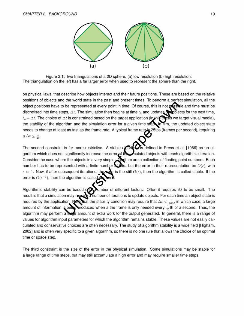
Most cases require a trade-off between the simulation error and the detail or speed of the simulation. Forexample, a 2D or 3D object can be represented as a triangle mesh. Figure 2.1 shows two possible representa-tions for a 2D circle with different levels of detail. The first samples the space on a grid of step size ∆x = 1 andthe second on a grid with ∆x = 0.5. The smaller step values allow representation of higher levels of details,with less error. However, at a higher level of detail, more information has to be stored and the trade-off isbetween detail and the memory required. In addition to the extra memory requirements, more triangles couldresult in more processing, if the complexity of the simulation algorithm is proportional to the number of triangles.

A simulation algorithm updates the object representations over time. The algorithm has rules, often based

18

Univers

ity of

Cap

e Tow

n

CHAPTER 2. BACKGROUND 19

Figure 2.1: Two triangulations of a 2D sphere. (a) low resolution (b) high resolution.The triangulation on the left has a far larger error when used to represent the sphere than the right.

on physical laws, that describe how objects interact and their future positions. These are based on the relativepositions of objects and the world state in the past and present times. To perform a perfect simulation, all theobject positions have to be represented at every point in time. Of course, this is not possible and time must bediscretised into time steps, ∆t. The simulation then begins at time t0 and updates the objects for the next time,to + ∆t. The choice of ∆t is constrained based on the target application (in this thesis we target visual media),the stability of the algorithm and the simulation error for a given time step. In film, the updated object stateneeds to change at least as fast as the frame rate. A typical frame rate is 25fps (frames per second), requiringa ∆t ≤ 1

25 .

The second constraint is far more restrictive. A stable algorithm is defined in Press et al. [1986] as an al-gorithm which does not significantly increase the error of the simulated objects with each algorithmic iteration.Consider the case where the objects in a very simple algorithm are a collection of floating point numbers. Eachnumber has to be represented with a finite number of bits. Let the error in their representation be O(ε), withε 1. Now, if after subsequent iterations, the error is the still O(ε), then the algorithm is called stable. If theerror is O(ε−1), then the algorithm is called unstable.

Algorithmic stability can be based on a number of different factors. Often it requires ∆t to be small. Theresult is that a simulation may require a number of iterations to update objects. For each time an object state isrequired by the application. Note that the stability condition may require that ∆t < 1

100 , in which case, a largeamount of information is being produced when a the frame is only needed every 1

25 th of a second. Thus, thealgorithm may perform a large amount of extra work for the output generated. In general, there is a range ofvalues for algorithm input parameters for which the algorithm remains stable. These values are not easily cal-culated and conservative choices are often necessary. The study of algorithm stability is a wide field [Higham,2002] and is often very specific to a given algorithm, so there is no one rule that allows the choice of an optimaltime or space step.

The third constraint is the size of the error in the physical simulation. Some simulations may be stable fora large range of time steps, but may still accumulate a high error and may require smaller time steps.

Univers

ity of

Cap

e Tow

n


2.2 Fluid Simulation

This section introduces some of the common concepts when dealing with fluids and the behaviour that is re-quired for people to believe that a simulation run on computer is actually real fluid.

A fluid is defined by Batchelor [2000] as a substance that, when pressure is applied, flows into a differentshape. Flowing is the free movement of the substance over time. A fluid may offer some resistance, which ismeasured by the viscosity of the fluid. The higher the resistance it offers, the higher the viscosity. A solid canbe regarded as fluid with infinite viscosity, as it does not flow at all when pressure is applied. Ideally, viscositywill be a parameter of the simulation and different fluids should be produced, based on this parameter. The unitof measurement for kinematic viscosity1 is m2s−1. There are many ways to describe viscosity, but they are allequivalent. Effectively, kinematic viscosity is a measure of how quickly a fluid will accelerate due to movementof surrounding fluid.

There are several other important quantities when considering fluid behaviour. The first is mass, or howheavy the fluid is. Conservation of mass is one of the most important physical constraints. A fluid simulationshould neither create or destroy fluid matter, except for cases where fluid is added to a scene, from a tap forexample, or removed from a scene, at a sink hole. The mass should remain constant from one time step tothe next, unless visual realism is the sole requirement, in which case the change in mass should be sufficientlysmall to be invisible.

Another quantity, already mentioned, is pressure, it is defined as force per unit volume. It describes the amountforce a quantity of fluid at a given position exerts on the fluid around it. The pressure can be different for everypoint in the fluid and is denoted by the scalar field P (x, y, z). When pressure is applied to a fluid from oneside, it will slowly be transmitted to the other side of the fluid over time due to the intermolecular forces. Alsoimportant for fluids is density, defined as the mass per unit volume. This is not necessarily constant, but we willonly be considering fluids with constant density for the purposes of this thesis. This family of fluids is known asincompressible fluids [Carlson, 2004]. Fluids such as water and oil are very close to being incompressible andit is mainly gases that are considered readily compressible. For the purpose of this thesis water and oil aretreated as incompressible. Finally, the physical parameter velocity describes the movement of a body of fluid .

These quantities can also be described at different spatial levels or scales, which represent the amount ofspatial detail being captured. The previous description of quantities is given at a macroscopic level, where onlyan aggregate behaviour of each of the underlying molecules is considered. At a microscopic scale the atomicinteractions are important. For pressure, this would be an expression describing the number of collisions persecond per unit area, as this would result in the corresponding forces per unit area on the macroscopic level.There is a third level, the mesoscopic level, which is in-between the macroscopic and microscopic levels. Thisconsiders a collection of molecules instead of just one. Some quantity representations may be more conve-nient at certain levels.

Fluids can be classified into two categories: Liquids and Gasses. Each of these categories has differentphysical characteristics. Most notably, a liquid has a free surface, which marks the presence or absence offluid and adds additional physical constraints, while a gas has no clear boundary. However, the underlyingfluid behaviour is the same, so the fluid simulation problem is split up into two parts: fluid velocity/pressure

1There are other definitions of viscosity, but this is the one most relevant to this thesis.

Univers

ity of

Cap

e Tow

n


simulation and fluid surface representation.

Turbulence is one of the most important effects to consider for realistic fluid behaviour. This describes thechaotic behaviour of a fluid. An example of turbulent behaviour is a large sea wave breaking on a shore. Thewater churns and is far from but a constant flow of water. Turbulent flow is characterised as a part of the flowthat has a highly differentiated and unpredictable pressure and velocity over a small space [Batchelor, 2000]. Agood simulation should be able to produce turbulent behaviour at full detail. Vortices are also often associatedwith turbulence. These are spinning flows of a fluid, such as when water flows down a drain.

So far, the fluid has been described in a very physical sense. From a more everyday perspective, a fluidis something that splashes, infinitely divisible, sticks to objects, forms whirlpools and flows. Another interestingfluid phenomenon is bubbles, where air is trapped inside the fluid, or foam, as seen on sea waves. Foamoccurs due to the surface tension of fluid. This is the attraction of the fluid surface to other fluid surfaces thatcauses a minimization of surface area [de Gennes et al., 2004]. The most common evidence of surface tensionis the formation of spherical drops when water falls. These are all effects a simulation should support.

Finally, we consider how fluid interacts with its environment, such as rocks and trees. Furthermore, obsta-cles provide a direct method of controlling fluid movement. The way in which the water interacts with obstaclesin the environment is defined in the boundary conditions. These conditions define how the fluid bounces orslips across an obstacle when they come in contact. It is possible to have very complex or simple boundaryconditions and the resulting fluid simulations can be very different [Poinsot and Lele, 1992].

2.3 First Approaches and the Navier-Stokes Equations

There were various early approaches to modelling fluids. These can be differentiated into those which seekphysical accuracy and those where the focus is on appearance. Many of the early approaches fall into the latercategory, as the computation power available was not sufficient for accurate simulations. In such cases, thephysical properties of fluids are not considered (or not all the properties). Rather, the authors seek to createsimilar behaviour to what would be seen with the human eye. Our application is visual effects and this thesisfocuses on similarly producing fluid that at least behaves as a person would expect. Of course, a physicallycorrect simulation will also look correct to the human eye.

The smallest physical building block that causes fluid behaviour is the particle and a fluid is a collection ofparticles. Each particle exerts forces, both attraction and repulsion, on neighbouring particles. This is a sim-plistic view of how a fluid behaves, but is sufficient to reproduce complex movement. Miller and Pearce [1989]used this idea as a basis for fluid simulation. Particles at a close distance repel each other and those at amoderate distance attract. The particles can then be accelerated with the sum of all the forces. To use thisapproach, all particles have to be simulated and all forces calculated.

Fluids can be modelled in other simple ways. For example, Fournier and Reeves [1986] used parametricfunctions to model ocean waves. They modelled the waves as they move across different ocean floors andadded particles to breaking waves, which take on the velocity given by the wave parametrization. This para-metric function makes use, in part, of sinusoidal functions, which were used in other earlier approaches [Fosterand Metaxas, 1996]. Sinusoidal functions are effective because they are wave functions, which are often as-

Univers

ity of

Cap

e Tow

n


sociated with fluid movement. The method is fast, but does not allow for highly detailed interactions with thefluid and the look of the fluid is limited to the shape of the function, which is unsuitable for film applications, asthe results are not realistic enough.

One of the more physically based approaches, applied by Kass and Miller [1990], makes use of shallow-water differential equations. These equations model the water in 21

2 dimensions -only a 2D plane of wateris simulated. The water surface is approximated as a height-field. They also modelled rain and beach waveeffects. Using these differential equations they produce a simple, stable method which only requires one sim-ulation iteration per frame of animation [Kass and Miller, 1990]. The stability of this method is good and theequations are simple, low in computation cost and the animations fast to produce. However, the fluid velocityis only known at the surface, which is a problem for a full 3D scene with submerged objects. Also, object-fluidinteractions are not taken into account and the model does not cater for full 3D fluid simulation.

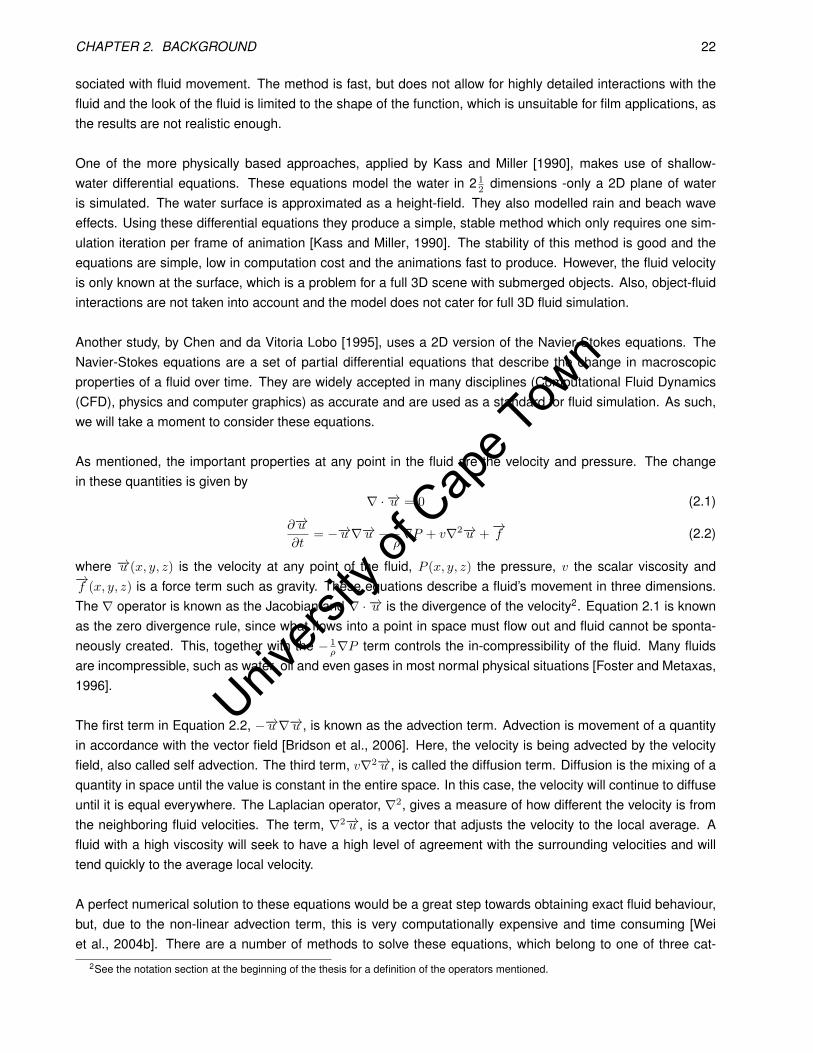
Another study, by Chen and da Vitoria Lobo [1995], uses a 2D version of the Navier-Stokes equations. TheNavier-Stokes equations are a set of partial differential equations that describe the change in macroscopicproperties of a fluid over time. They are widely accepted in many disciplines (Computational Fluid Dynamics(CFD), physics and computer graphics) as accurate and are used as a standard for fluid simulation. As such,we will take a moment to consider these equations.

As mentioned, the important properties at any point in the fluid are the velocity and pressure. The changein these quantities is given by

∇ · −→u = 0 (2.1)

∂−→u∂t

= −−→u∇−→u − 1

ρ∇P + v∇2−→u +

−→f (2.2)

where −→u (x, y, z) is the velocity at any point of the fluid, P (x, y, z) the pressure, v the scalar viscosity and−→f (x, y, z) is a force term such as gravity. These equations describe a fluid’s movement in three dimensions.The ∇ operator is known as the Jacobian and ∇ · −→u is the divergence of the velocity2. Equation 2.1 is knownas the zero divergence rule, since what flows into a point in space must flow out and fluid cannot be sponta-neously created. This, together with the − 1

ρ∇P term controls the in-compressibility of the fluid. Many fluidsare incompressible, such as water, oil and even gases in most normal physical situations [Foster and Metaxas,1996].

The first term in Equation 2.2, −−→u∇−→u , is known as the advection term. Advection is movement of a quantityin accordance with the vector field [Bridson et al., 2006]. Here, the velocity is being advected by the velocityfield, also called self advection. The third term, v∇2−→u , is called the diffusion term. Diffusion is the mixing of aquantity in space until the value is constant in the entire space. In this case, the velocity will continue to diffuseuntil it is equal everywhere. The Laplacian operator, ∇2, gives a measure of how different the velocity is fromthe neighboring fluid velocities. The term, ∇2−→u , is a vector that adjusts the velocity to the local average. Afluid with a high viscosity will seek to have a high level of agreement with the surrounding velocities and willtend quickly to the average local velocity.

A perfect numerical solution to these equations would be a great step towards obtaining exact fluid behaviour,but, due to the non-linear advection term, this is very computationally expensive and time consuming [Weiet al., 2004b]. There are a number of methods to solve these equations, which belong to one of three cat-

2See the notation section at the beginning of the thesis for a definition of the operators mentioned.

Univers

ity of

Cap

e Tow

n


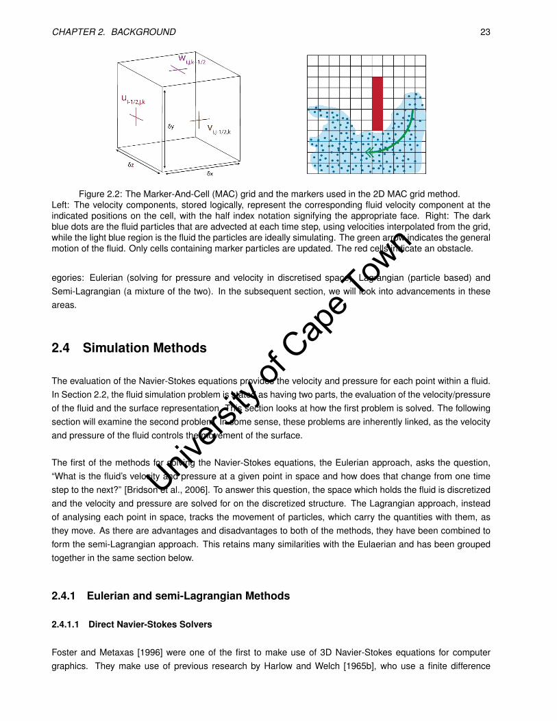
Figure 2.2: The Marker-And-Cell (MAC) grid and the markers used in the 2D MAC grid method.Left: The velocity components, stored logically, represent the corresponding fluid velocity component at theindicated positions on the cell, with the half index notation signifying the appropriate face. Right: The darkblue dots are the fluid particles that are advected at each time step, using velocities interpolated from the grid,while the light blue region is the fluid the particles are ideally simulating. The green arrow indicates the generalmotion of the fluid. Only cells containing marker particles are updated. The red cells indicate an obstacle.

egories: Eulerian (solving for pressure and velocity in discretised space), Lagrangian (particle based) andSemi-Lagrangian (a mixture of the two). In the subsequent section, we will look into advancements in theseareas.

2.4 Simulation Methods

The evaluation of the Navier-Stokes equations provides the velocity and pressure for each point within a fluid.In Section 2.2, the fluid simulation problem is stated as having two parts, the evaluation of the velocity/pressureof the fluid and the surface representation. This section looks at how the first problem is solved. The followingsection will examine the second problem. In some sense, these problems are inherently linked, as the velocityand pressure of the fluid controls the movement of the surface.

The first of the methods for solving the Navier-Stokes equations, the Eulerian approach, asks the question,“What is the fluid’s velocity and pressure at a given point in space and how does that change from one timestep to the next?” [Bridson et al., 2006]. To answer this question, the space which holds the fluid is discretizedand the velocity and pressure are solved for on the discretized structure. The Lagrangian approach, insteadof analysing each point in space, tracks the movement of particles, which carry the quantities with them, asthey move. As there are advantages and disadvantages to both of the methods, they have been combined toform the semi-Lagrangian approach. This retains many similarities with the Eulaerian and has been groupedtogether in the same section below.

2.4.1 Eulerian and semi-Lagrangian Methods

2.4.1.1 Direct Navier-Stokes Solvers

Foster and Metaxas [1996] were one of the first to make use of 3D Navier-Stokes equations for computergraphics. They make use of previous research by Harlow and Welch [1965b], who use a finite difference

Univers

ity of

Cap

e Tow

n


scheme coupled with a Marker-And-Cell (MAC) grid to evaluate the equations. A MAC grid stores the fluidvelocities at the face centres for each face of a grid cell (see Figure 2.2). The pressure is stored at the centerof the cell. For each time step, the following finite difference equation is used [Foster and Metaxas, 1996]:

u∗i+1/2,j,k = ui+1/2,j,k + δt1

δx[u2i,j,k − (ui+1,j,k)2]

+1

δy[(uv)i+1/2,j−1/2,k − (uv)i+1/2,j+1/2,k]

+1

δz[(uw)i+1/2,j,k−1/2 − (uw)i+1/2,j,k+1/2]

+1

δx(ρi,j,k − ρi+1,j,k)

+v

δx2(ui+3/2,j,k − 2× ui+1/2,j,k + ui−1/2,j,k)

+v

δy2(ui+1/2,j+1,k − 2× ui+1/2,j,k + ui+1/2,j−1,k)

+v

δz2(ui+1/2,j,k+1 − 2× ui+1/2,j,k + ui+1/2,j,k−1) (2.3)

where u∗ is the x-component of the velocity for the next time step. The symbols u, v, w are the x, y, z com-ponents, respectively, of velocity for the current time step and δx, δy, δz are the grid resolutions along therespective axes. The equation seeks to solve the Navier-Stokes differential equation by stepping throughspace and time in finite increments. The 1/2 indices denote one of the face positions. For the algorithm toremain stable max[u δtδx , v

δtδy , w

δtδz ] < 1 [Foster and Metaxas, 1996]. For this method, an increase in the spatial

resolutions requires an increase in time resolution of the algorithm and vice versa. The more detail required,the higher the computation cost. Using this given condition, to simulate fluid flowing at 1ms−1 at a scale of1mm, δx = 0.001m, would require a time step of less then 0.001s. Far more simulation steps would be requiredthan animation frames generated.

After Equation 2.3 has been used to update the velocities, the velocity field may no longer have zero di-vergence. For a particular cell, this is corrected by using a similar finite difference form of Equation 2.1, whichadjusts the pressure of a cell to counter the divergence created by the first step. Cell velocities are then ad-justed according to the pressure. Adjusting one cell may affect a neighboring cell, so this is repeated for eachcell. Foster and Metaxas [1996] conclude that their method has a high computational cost of O(n4), where nis the the number of cells along one axis of the grid.

As the previous method requires a large number of extra simulation steps to remain stable, Stam [1999]introduces an unconditionally stable semi-Lagrangian method. The method is unconditionally stable since anysize time-step may be used and the simulation error remains bounded. His method splits up the solution of theNavier-Stokes equations into four steps (each step updates the velocity field). First the external force is usedto accelerate the velocity field:

u1(~x) = u0(~x) +4tf(~x).

Then the velocity field is updated by self advection. During a time-step, 4t, the velocity field will advect fluidaround. The field at ~x(t) is updated by tracing a particle from ~x back through time, along the field lines, to itsposition at the previous time, t−4t. The value of the velocity field at this position is used, namely

u2(~x) = u1(~x(t−∆t)).

Univers

ity of

Cap

e Tow

n


Thirdly, the velocity is diffused by solving the linear system:

(I − v4t∇2)u3(~x) = u2(~x).

The system is solved for u3(−→x ), using a partial differential equation solver. Lastly, the velocity field is correctedto make sure it has zero divergence. The Helmholtz-Hodge Decomposition states that any vector field can bedecomposed into the sum of a divergence free vector field and a scalar field. Using this result, Stam [1999]projects the velocity onto a field with zero-divergence, by converting the projection into a sparse linear system,solvable in linear time. This is a global projection, as the entire velocity field must be known and projected.

The approach by Stam [1999] has become very popular and it, or its variations, are used by Fedkiw et al.[2001], Foster and Fedkiw [2001], Foster and Metaxas [1996], Carlson et al. [2004], Fattal and Lischinski[2004], Irving et al. [2006] and Losasso et al. [2006b]. However, due to the first order integration required, theapproach suffers from numerical dissipation [Fedkiw et al., 2001], which causes fluids to be less turbulent thenthey are in reality.

To inject the energy lost to numerical dissipation into the field, Fedkiw et al. [2001] introduce “vorticity con-finement” to computer graphics; the idea comes originally from CFD literature. They give the measure of thevorticity as the curl of the velocity field, ω = ∇ · −→u , and add a forcing term to Equation 2.2 proportional to thismeasure. The authors claim that this method agrees with the full Navier-Stokes equations, but the magnitudeof the forcing term has to be kept small for a stable simulation. A similar idea is used by Selle et al. [2005],but they use vortex particles to enhance the details of the fluid, where each particle carries a vorticity value.Particles are placed in the fluid flow at any point and use the velocity of the flow and the vorticity form of theNavier-stokes equations 3,

ωt + (−→u · ∇)ω − (ω · ∇)−→u = v∇2ω +∇× f, (2.4)

to evolve the particle positions and vorticity values, respectively, over time. Later, the vorticity at a point in thefluid is calculated by a weighted average of the nearby particles and energy is injected back into the fluid in asimilar fashion to Fedkiw et al. [2001]. An application of these particles is given in Irving et al. [2006], wherethe vortex particles are placed behind a boat to add turbulence as it travels through water.

Currently, a 3D grid or voxel structure is required for an Eulerian simulation and the detail of the simulationis limited to the resolution of the grid. Some scenes may have different regions of detail, indeed, parts of thescene may be completely empty. Losasso et al. [2004] use an octree structure in place of the regular grid,with increased detail over certain regions. They show enhanced smoke simulation around a sphere, an objecttypically difficult to embed in a grid. Irving et al. [2006] use a height field structure for fluid below a surface,coupled with a full 3D grid on the surface. The structure is justified, as most detail will occur on the surface andthe sub-surface level effects will be smoothed and less noticeable.

Departing from the traditional grid-based evaluations of the Navier-Stokes equations, many authors employtetrahedral meshes. The grid based approach does not work well with irregularly shaped obstacles. Feld-man et al. [2005a] improve the interface between a regular grid and objects by filling the gap with tetrahedralmeshes. Similar to the design of the MAC grid, the velocity values are defined at the faces of the tetrahedron

3Obtained by taking the curl, ∇×, of Equation 2.2.

Univers

ity of

Cap

e Tow

n


and the pressure at center. Klingner et al. [2006] generalises the stable method of Stam [1999] to tetrahedralmeshes. As the obstacles are rarely static, Klingner et al. [2006] present a method for smoke animation thatgenerates a new mesh for each iteration of the algorithm. The velocity values are transferred onto the newmesh using the semi-Lagrangian advection of Feldman et al. [2005b]. The pressure correction and forcingterms of the Navier-Stokes equations are then taken into account.

In conclusion, the direct Navier-Stokes solvers provide an unconditionally stable numerical scheme and al-low arbitrary time steps to be used for the simulation. This has considerable advantages, as the speed ofthe simulation is not reduced by unneeded iterations. The most advanced and visually compelling simulationshave been produced using the grid based solvers based on the method of Stam [1999].

The method, however, relies on a global pressure correction step to enforce incompressibility and this, un-fortunately, increases the cost for conversion to a parallel architecture. Being a grid based approach, objectinteractions have to be translated into the grid structure, introducing possible boundary errors. Also, sub-grideffects, such as foam, cannot be modelled by the system.

2.4.1.2 Indirect Navier-Stokes Solvers using Cellular Automata methods

A cellular system is defined by Wolf-Gladrow [2000] as a “regular arrangement of single cells” with similar cellproperties. These cells have states which change in discrete time steps. The rules that govern the changeof state of a cell depend only on neighbouring cells. A cellular automata to describe fluid movement dividesa region up into cells that cover the entire fluid and provide rules that update physical properties of each cell,such that the resulting physical behaviour will obey the Navier-Stokes equations.

The previous Eulerian approach simulated fluid from a macroscopic point of view. The alternative approachtaken is to model the dynamics that produce the correct fluid behaviour. The fluid is now modelled at a meso-scopic level. We begin with the early methods in lattice cellular automata.

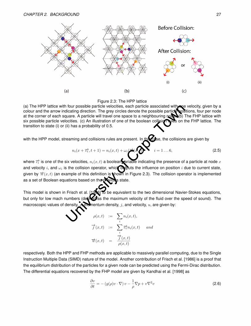
The first of the Lattice-gas cellular automata is called the HPP model (after the initials of the authors) andwas introduced by Hardy et al. [1976]. This two dimensional method evenly divides up the region into squares,with a node placed at each corner (see Figure 2.3). Each node can hold four particles, which travel along oneof four possible velocities to one of the neighbouring nodes. The particles, in effect, represent a collection ofatoms. The model defines a collision operator and a streaming operator. The collision operator resolves theinteraction of particles at a node, while the streaming operator propagates particles to neighbouring nodes.

The HPP model conserves mass and momentum [Kandhai et al., 1998], but fails to reproduce the macro-scopic effects of the Navier-Stokes equations, due to the lack of rotational invariance [Wolf-Gladrow, 2000,Succi, 2001, Kandhai et al., 1998], as a rotation of the lattice yields different results for macroscopic values.Succi [2001] states that he also found that the method produced square vortices. Instead of the usual circularshape, the vortices have four flat edges that line up with the lattice.

Frisch et al. [1986] introduce the FHP model, which overcomes the lack of rotational invariance by dividingup the space into triangles and placing the nodes of the lattice on the corners of the triangles, giving the latticehexagonal symmetry (see Figure 2.3), as each node is connected to six other nodes. Again, each node hassix possible positions for particles, each of which can travel along one of the six possible velocity vectors. As

Univers

ity of

Cap

e Tow

n


Figure 2.3: The HPP lattice(a) The HPP lattice with four possible particle velocities, each particle associated with one velocity, given by acolour and the arrow indicating direction. The grey circles denote the possible particle positions, four per nodeat the corner of each square. A particle will travel one space to a neighbouring node. (b) The FHP lattice withsix possible particle velocities. (c) An illustration of one of the boolean collision rules on the FHP lattice. Thetransition to state (i) or (ii) has a probability of 0.5.

with the HPP model, streaming and collisions rules are present. In this case, the collisions are given by

ni(x+−→ci , t+ 1) = ni(x, t) + ωi(−→n (x, t)) i = 1 . . . 6, (2.5)

where −→ci is one of the six velocities, ni(x, t) a boolean variable indicating the presence of a particle at node xand velocity i, and ωi is the collision operator, which outputs the influence on position i due to current state,given by −→n (x, t) (an example of this definition is shown in Figure 2.3). The collision operator is implementedas a set of Boolean equations based on the previous state.

This model is shown in Frisch et al. [1986] to be equivalent to the two dimensional Navier-Stokes equations,but only for low mach numbers (defined as the maximum velocity of the fluid over the speed of sound). Themacroscopic values of density, ρ, momentum density, j, and velocity, u, are given by:

ρ(x, t) :=∑i

ni(x, t),

−→j (x, t) :=

∑i

−→cini(x, t) and

−→u (x, t) =−→j (x, t)

ρ(x, t)

respectively. Both the HPP and FHP methods are applicable to massively parallel computing, due to the SingleInstruction Multiple Data (SIMD) nature of the model. Another contribution of Frisch et al. [1986] is a proof thatthe equilibrium distribution of the particles for a given node can be predicted using the Fermi-Dirac distribution.The differential equations recovered by the FHP model are given by Kandhai et al. [1998] as

∂v

∂t= − (g(ρ)v · ∇) v − 1

ρ∇p+ v∇2v (2.6)

Univers

ity of

Cap

e Tow

n


These are similar to the Navier-Stokes equations, except for the g(ρ) = ρ−3ρ−6 factor. However, for low mach

numbers, time can be re-scaled, i.e. t∗ = tg(p) [Wolf-Gladrow, 2000] and the full equations can be recovered

with a scaling of the viscosity, v∗ = vg(ρ) . Hence, an adjustment to the required viscosity needs to be made.

Other improvements to the model were made by introducing a rest particle for each node. This is known asthe FHP II model [Frisch et al., 1987] and further modifications made to the collision operator in FHP III, allowthe use of larger range of mach numbers. The drawback of the FHP methods is that the simulations producenoise artifacts and, to obtain pleasing results, the average over a large number of repetitions of the algorithmhas to be used [McNamara and Zanetti, 1988]. This has a large computational requirement.

McNamara and Zanetti [1988] introduce the first of the Lattice-Boltzmann methods. They no longer useBoolean variables, ni, for the presence of particles, but track the average value of the particle distributions,fi, by using real numbers between 0 and 1. The collision operator is the same as the FHP model, but nowsubstitutes the arithmetic operations “+” and “.” for the Boolean operators “and” and “or” used by Frisch et al.[1987]. The use of particle distributions avoids statistical noise, hence the method is more efficient. As withthe FHP model, the collision operator is a non-linear function of all possible particle positions at a node and iscomputationally expensive. To reduce the computational complexity, Higuera and Jiménez [1989] produce aquasi-linear collision operator. The operator gives the change of a given fi as a linear combination of all thecurrent node distribution functions. This advance is seen by Succi [2001] as the "most significant breakthroughin LBM theory" as simulations now become computationally practical.

The current linear combination of fi, for all i, is derived from the rules in FHP, which state when a collisioncan occur between particles traveling along given velocities. These rules were chosen in such a way as toconserve momentum and mass and to give rise to the Navier-Stokes equations. Higuera et al. [1989] showthat they are not the only rules that generate the equations and that other linear combinations still produce fluidbehaviour. They effectively allow the simulation of flows with far lower viscosities than previous methods.

The collision operator was simplified even further by Qian et al. [1992], who use a relaxation technique inplace of the operator. They use the equilibrium distribution,

fei (t, x) = tpρ

1 +

ci · −→uc2s

+uαuβ2c2s

(ciαciβc2s

− δαβ)

,

to give fei for a given velocity, −→u . Here, cs is the speed of sound, tp is a weighting value to retain latticesymmetry (see paper for details) and α, β denotes the sum over Cartesian coordinates. Collisions are thenresolved using the following:

fi(x, t+ 1) = (1− ω)fi(x, t) + ωfei (x, t). (2.7)

This operator only relies on one distribution function, the equilibrium distribution and the parameter ω. This isknown as a relaxation method, as the current distribution, fi, is relaxed towards equilibrium, fe. The LatticeBoltzmann Method is based on this movement of particles from one cell to neighbouring cells and this collisionoperator.

The LBM was introduced into computer graphics by Thürey [2003], based on the use of LBM in metal foamingfrom Körner and Singer [2000] and Körner et al. [2002]. In these papers, the method is validated and testedagainst real fluids, such as a breaking dam experiment. Thürey [2003] is able to produce simulations of fallingdrops, breaking dams and bubbles rising in water. The stability of the simulations is not discussed extensively,but very small bounded time steps are required and stability problems are reported for low viscosities. The time

Univers

ity of

Cap

e Tow

n


step in the lattice is limited by the fluid velocity as a fluid particle cannot travel more then one grid space persimulation iteration. If the step is too large collisions can no longer be resolved in a physically correct mannerand the simulation becomes unstable.

With a fixed time step, the velocity of the fluid may become large and cause instabilities. Thürey et al. [2006]improve the stability of the simulation by introducing adaptive time steps. When the maximum velocity of thefluid is detected to be too large, the simulation is re-parametrized with respect to a new smaller time step.The new parametrization gives new lattice viscosities, such that the behaviour of the fluid at the new time stepwill agree with its previous behaviour and higher overall velocities can be simulated. Using this more stablealgorithm, Thurey et al. [2005a] produce interactive free-surface simulations on grid sizes of 263 to 363, runningat frame rates of 20-27 fps on a standard desktop PC.

To improve the performance of the LBM, Thürey and Rüde [2005] use an adaptive grid. Groups of LBMcells are aggregated in regions of low interest into one larger LBM cell. The interface between the large celland smaller cells is modified to maintain correct behaviour. This approach reduces the running time of sim-ulations by a third for the falling drop and breaking dam test cases. The use of larger grid sizes, however, isa new source for instabilities as the large grid can no longer resolve sub-grid turbulence. Thürey and Rüde[2008] use a sub-grid turbulence model to resolve the instabilities and produce high quality stable animationswith approximately a 3.85 times improvement in speed.

In summary, the cellular automata methods provide a simple cellular automata style fluid representation, withequally simple update rules. During an update, only local information is needed and the method is inherentlyparallizable, as work units can be distributed to different locations (threads, processes or CPUs) and the costof quantity synchronization will be low. This makes the possibility of parallel conversion straightforward. Com-plex boundary conditions are handled simply and quickly, as the particle distributions can individually interactwith objects. Simple boundary conditions offer adequate fluid simulations, but there is room for improvement.Shankar and Sundar [2009] show that the solution obtained from the LBM simulation can be improved withmore complex boundary conditions.

The LBM methods are applicable to computer graphics, but are very memory intensive, as they need to store alarge amount of information for each grid cell. This is a drawback when modelling large scenes. The numericalscheme is not unconditionally stable for fluids with low velocities, so an adaptation needs to be used to intro-duce stability with a consequent added computation cost. Additionally, a maximum fluid velocity is imposed toensure stability.

2.4.2 Lagrangian Methods

The Lagrangian methods use particles to represent the fluid. These particles carry all the fluid quantities withthem as they travel through space. Mass is explicitly defined for each particle and mass is always conservedas the number of particles remains constant. Density is then related to the number of particles per unit volume,while pressure and velocity, for each particle, are then related to the surrounding particles. This is the generalapproach to handling Lagrangian fluids with particles, but some methods may have more specific or differentapproaches.

Univers

ity of

Cap

e Tow

n


Figure 2.4: Fluid simulated using Smoothed Particle Hydrodynamics (SPH).(a) The traditional SPH representation with uniform sized particles. (b) The multi-resolution SPH method withvarying sized particles. Both show the rigid floating duck. A rigid object is populated with particles that formthe basis for the object’s interactions in the scene.

Smoothed Particle Hydrodynamics (SPH) treats the volume of a fluid as a collection of small regions andwas first introduced to the graphics community for fluid simulation by Müller et al. [2003]. SPH embeds parti-cles into a scene where fluid is present, and these particles are advected using the Navier-Stokes equationsto calculate their acceleration, see Figure 2.4 (a). Each particle represents a small element of fluid, with massmj at position −→rj . The key to this method is the calculation of smoothed values of density and relative velocityover the collection of particles. The smoothed density field of a quantity, As, at −→r is given as the sum of allparticle contributions, weighted by a kernel function, W , (such as a Gaussian distribution)

As(−→r ) =∑j

mjAjρjW (−→r −−→rj , h) . (2.8)

In the equation, Aj is the value of the quantity for particle j. The integral of the kernel function is normalizedto 1, to ensure that no loss of mass occurs. The parameter h selects the influence radius of each particle;the further a particle is from another the less influence it has. An advantage to using particles is that massis perfectly conserved and Equation 2.1 can be omitted, although this does introduce some compressibilityeffects. Furthermore, the advection term of Equation 2.2, −u∇u, can also be omitted as the particles areadvected for each step of the simulation and this term is handled implicitly by the representation. With thesesimplifications, the acceleration of the particle i is

−→ai =d−→vidt

=1

ρ

(−∇P + ρ

−→f + µ∇2−→u

). (2.9)

First the density for each particle is calculated using the smoothed density field equation, as this depends onlyon the mass and the kernel function. Then, the smoothed quantities P and −→u are calculated using Equation2.8. An adjustment is needed to make the pressure and viscosity force symmetric between any two particles,making the method non-exact. Some details have been omitted and the interested reader is referred to theoriginal paper. The author produces interactive simulations with frame rates of 25 fps and 5fps for water in aglass, but the surface of the water is “blobby” and unrealistic.

To improve previous results, the moving particle semi-implicit method (MPS) uses a very similar definitionand algorithm to the SPH method, but includes an extra pressure correction step to ensure in-compressibility[Premoze et al., 2003]. This pressure correction mimics that of Stam [1999]. The MPS approach producesfluid simulations in a run time of about 3-4 minutes per frame of animation with 100 000-150 000 particles ona Pentium 4 1.7Ghz with 512Mb RAM. The final results look more realistic than Müller et al. [2003], but this isexpected with a far higher particle count.

Univers

ity of

Cap

e Tow

n


Keiser et al. [2006] introduce a multi-resolution particle approach, where a group of particles are representedas one particle, see Figure 2.4 (b). With this approach, they achieve a 6 times speedup, for some examples,over the single resolution method. However, for simulations of turbulent fluid, most of the fluid has to be repre-sented at the finest resolution. For such cases, no matter which approach one uses, very fine data structureswill be needed to properly simulate fluids, as the dynamics that produce the fluid movement only happen on avery small scale.

The authors also use a unified approach to modelling solid objects in the scene by sampling the objectswith particles. The fluid particles then exert a force on each of the object particles and the combined forcesthen give the transformation of the rigid body. Rigid body-on-rigid body collisions are handled in the same way,by calculating the effect of particle collisions belonging to each body.

In conclusion, the Lagrangian methods conserve mass perfectly, and they are not confined to specific gridlocations. The method is easily parallizable, as each of the particle updates are independent. Indeed, due thekernel function in the smoothed quantities, the influence can even be zero beyond a certain distance, makingonly locally close particles important during the update step. The particle approach also lends itself nicely tofluid-fluid interactions [Müller et al., 2005], deformable objects [Keiser et al., 2005] and representation of effectssuch as bubbles and foam [Losasso et al., 2008]. The particle methods can be coupled with other methods.Losasso et al. [2008] show that the popular Eulerian approach can be augmented with SPH particles to modelfoam and bubbles, which cannot be simulated on a grid.

The disadvantages of the particle methods are in the look and feel of the liquid. Once the particle positionshave been simulated, the surface of the fluid must be generated. In general, it is hard to generate a smoothsurface from particles and a large number of particles are required to make the simulation realistic [Thurey,2007]. Simulations generated using the particle methods do not look as good as simulations using the Eulerianmethods. Compressibility is, in general, allowed in these simulations, unless a costly pressure-correction stepis used.

2.5 The Fluid Surface

There are many methods of representing the fluid surface. A common approach uses marker particles on theMAC grid [Harlow and Welch, 1965a, Foster and Metaxas, 1996], which show where the fluid exists in space(see Figure 2.2 (b)). The collection of all the particles is then used to represent the fluid surface. For eachiteration, the particles are moved using the velocity of the fluid. Foster and Metaxas [1996] instead use aheight-field to represent the surface of a liquid. Stam [1999] uses marker particles to indicate the occurrenceof smoke in a scene, but use a combination of advected texture co-ordinates and density values to render thesmoke.

Foster and Fedkiw [2001] define a particle level set, which uses particles to define the surface of a liquid.An implicit function is created, φ(x), which is defined by finding the closest particle to −→x and then subtractinga given radius, r, from

√(−→x −−→xp)2, where −→xp is the center of the particle. The liquid surface is generated by

sampling φ(x) on a grid and using the marching cubes algorithm to tessellate the φ(x) = 0 iso-contour with

Univers

ity of

Cap

e Tow

n


polygons. Both the particles and the level-set position are updated for each iteration. φ is updated using

φt + u · ∇φ = 0 (2.10)

and the particles using the fluid velocity. Level sets are prone to volume loss [Foster and Metaxas, 1996,Foster and Fedkiw, 2001] due to the finite difference approximation needed to calculate the update given byEquation 2.10. To fix this, regions of φ(x) with large curvature, indicating a region of splashing, are built usingthe particle’s position to alter the level-set. This gives a nice smooth surface for the whole liquid, in general,while regions of greater turbulence are represented with greater accuracy and effects such as splashing andfoam can be modelled. The method only uses particles within the fluid.

The level set approach of Foster and Fedkiw [2001] focuses on modelling the liquid volume. Due to theproblems with level sets, Enright et al. [2002] instead focus on the surface of the liquid to achieve more photo-realistic effects, which they regard as more important for application to movies. They build on work by Fosterand Fedkiw [2001] using the same approach to develop the water’s surface, but instead of using either thetessellated surface at φ = 0 or the particle positions to represent the liquid surface, they use the particles aserror correction term to the implicit function. In addition, particles are placed on the inside and outside of thefluid. This allows them to more correctly model phenomenon such as bubbles.

An alternative to the level set approach is the Volume of Fluid (VOF) method. Essentially, these methodstrack the fluid fill-fraction for each voxel in a grid. A fluid is given by a fraction of 1, while a gas is given by afraction of 0. The advantage of VOF is that mass can be perfectly conserved, however, it is difficult to get andaccurate curvature estimate [Bargteil et al., 2006]. The VOF method is used by Thürey [2003] in conjunctionwith the LBM method as the distribution functions of a lattice cell can be directly used to compute the exchangeof fluid from one voxel to another.

Sussman [2003] combine the level set and VOF techniques to represent the fluid surface. Thin sheets offluid can then be simulated and the volume preserved. Their method allows for higher accuracy, which in turnallows the use of lower grid resolutions, giving an increase in performance. However, the method still requiresthe VOF and level set calculations, which introduces significant overheads [Zhu and Bridson, 2005].

Lastly, in the case of Lagrangian simulations, a fluid surface can be built around particles in the simulation.This is done in a similar fashion to the level set implicit function, but for each frame of the animation. Mülleret al. [2003] use point splatting and iso-contouring to create the fluid surface. Keiser et al. [2005] use simplesurface particles called surfels that are small disk like objects oriented away from nearby associated particleswithin the SPH simulation. The surfels positions are updated using the associated particles movement. Thefluid is rendered by standard point sampled object rendering techniques. Keiser et al. [2006] create a smoothdynamic surface using a Delaunay triangulation between the particles withing the SPH simulation and air par-ticles placed on the outer edge of the fluid. The triangulation is simple and adapts to the resolution of thesimulation.

Univers

ity of

Cap

e Tow

n


2.6 Parallel Programming

This section introduces parallel simulations, parallel programming models, LBM parallelizations and technolo-gies (Subsections 2.6.1 to 2.6.4, respectively). The first subsection provides some of the general problems andalgorithm classifications for parallel simulations, while the second gives definitions for analysing and buildingprogramming models to predict program run times. The third looks at previous approaches used in conjunctionwith the LBM and the last describes some of the technologies that can be used for the parallel implementationof a simulation.

2.6.1 Parallel Simulations

As described in Section 2.1, a simulation consists of object representations that are updated for a numberiterations based on other objects and state information. To parallelize a simulation, the algorithm must be wellunderstood and the data dependencies between objects and state for each of the algorithm steps must becarefully considered. Parallel programs are limited by data dependencies, as they restrict the number of oper-ations that can be executed concurrently. The more dependencies between objects, the more synchronisationrequired. Fujimoto [2001] classifies synchronisation into conservative and non-conservative approaches. Aconservative approach ensures that all dependencies are met before performing an object update, while anon-conservative approach allows outdated data during an update step. Using outdated data may increasethe error in the simulation. More synchronisations per iteration, in the conservative approach, will cause a slowdown in the simulation, so a trade-off between simulation accuracy and speed is sometimes present.

It may be necessary to synchronise each process with every other process. This can be achieved throughdirect communication with all other processes or through a dependency chain. For example, a chain is createdwhen process k needs to synchronise with process k+ 1 and process k+ 1 in turn must synchronise with pro-cess k+ 2 and so on. The result is that process k has to wait for the last process to finish its work before it cancontinue its computation, and one iteration of the simulation is as slow as the slowest process in the chain. Tominimise the synchronisation times in such cases, the workload of all process must be kept as even as possible.

Different algorithms require different types of parallelization [Ramanathan et al., 2006]. The easiest to con-vert are the so called embarrassingly parallel algorithms. This class allows the update of simulation objectsentirely independently of one another. The second class is coarse-grained applications, in which entire loopsor functions are run on separate CPU’s. Third is the fine grained class, in which low level operations are run inparallel using special operations. This class uses features such as streaming SIMD Extensions (SSE) vectorinstructions that can perform many floating point instructions for a single clock cycle.

2.6.2 Parallel Programming Models

A model of the program provides a good way of understanding problems that may be encountered and poten-tial speed optimisations. Aoyama and Nakano [1999] provide a good model for analysis of any program beingparallelized. Every program is made up of a part that is inherently sequential and a part that is parallelizable.The parallelizable portion is a section of code that can be split up to run on multiple CPUs. The split canfollow the Single Program Multiple Data (SPMD) model or the Multiple Program Multiple Data (MPMD) model

Univers

ity of

Cap

e Tow

n


according to Flynn’s taxonomy [Flynn, 1972]. The first works well when there are many data items that can beupdated independently and the second when different algorithms need to be executed on the same data. Anexample of an un-parallelizable program is one in which the update of each data item requires all data itemsand they can only be updated in sequence.

Once we have identified which portion of the program is parallelizable, we can begin to determine how wellit will run on multiple CPUs. The total run time of a program is referred to as the wall clock time. This timecan be expressed as TTOT = Ts + Tp, where Tp is the portion of computation that can be parallelized andTs is the remaining portion that has to run on one CPU. Now, if the program is run on N CPUs, in the idealcase, TTOT = Ts +

Tp

N [Amdahl, 1967]. Unfortunately, communication time, denoted by Tc, which is needed tosynchronize the CPUs, adds to the overhead. Our final model is then

TTOT = Ts +TpN

+ Tc.

This gives rise to Amdahl’s law [Dongarra et al., 2003], which provides a lower bound on the run time for aprogram, namely TTOT > Ts.

While the total run-time of the program is a good indication of the parallel performance, an analysis method isneeded to determine how scalable and efficient the program is. System scalability is the measure of how muchfaster the program runs when using many CPUs. The first step for scalability studies is to ensure the singleCPU implementation is running correctly and efficiently. To get a base line run time for scenes, the run time ofthe single CPU simulation is used, and this is compared to the run time on N CPUs. The standard definition[Dongarra et al., 2003] of speedup for the multi-CPU implementation is calculated as

Speedup =TsingleTN

,

where Tsingle is the time for the single CPU implementation and TN the time for N CPUs. Tsingle is differentfrom T1, which is the time taken for the multi-CPU implementation running on 1 CPU. A plot of speedup versusnumber of CPUs will show how well the implementation divides the workload. The definition of efficiency forthe algorithm is calculated as

Efficiency =1

N× Speedup (2.11)

and indicates how well the simulation divides over N CPUs. A perfect distribution would give an efficiencymeasure of 1.

The communication time can be refined further, so that Tc = Tstart−up + nTdata. The first portion is the la-tency time, Tstart−up, required for handshakes and buffer set up. The buffer is required to optimise transfertime by storing data and sending it when the network becomes available. This way the program does not haveto wait for a slow network connection and can continue processing asynchronously while the send happens.This process is also used to overlap computation and communication. Finally, the time taken to send the bufferis given by nTdata, where n is the size of the data in bytes and Tdata is the time to send one byte of data. Whendesigning message sends, one can optimise them to take into account these values, but results may vary fordifferent architectures.

Amdahl’s law does not hold in some circumstances and superlinear speedup is achievable. A superlinearspeedup occurs when, for N CPUs, the speedup achieved is greater then N . Beane [2004] shows the cases

Univers

ity of

Cap

e Tow

n


where Amdahl’s law does not hold are due to multiple levels of cache, most notably the “on-chip” cache. Asmore CPUs are used, each with their own cache, it is possible for the entire data and program to fit into L1cache and the cache misses that occur with lower numbers of CPUs are circumvented. The author gives fourproperties that an algorithm must have to improve the probability of achieving superlinear speed-up. The first isthat the algorithm must iterate many times over a large data-set. Secondly, the parallel workload for each CPUmust diminish proportionally with the number of CPUs. Thirdly, Ts + Tc must be low and, lastly, super linearspeedup is more likely if the algorithm uses out of order memory accesses. Superlinear speed up is demon-strated by Venkatesh et al. [2004], who report a speedup of 11.05 for parallel CFD code on 8 processes, a37.5% super linear speedup.

2.6.3 LBM Parallelizations

A multi-CPU algorithm should evenly balance the processing load and assign portions of work to each availableprocessor, weighted according to their processing power, while minimizing the communication cost. Variousload balancing methods have been designed with this goal in mind. Some methods are static, where the loadis only balanced at the start of the simulation, while others are dynamic and the load balance changes duringthe run time of the simulation. Fluid motion introduces additional difficulties and the load balancing schememust be able to change work division dynamically to account for the fluid’s positional changes.

For LBM methods without free surfaces, a popular method for work assignment is domain decomposition,in the form of the slice, box and cube methods [Desplat et al., 2001, Amati et al., 1997, Pohl and Rüde, 2007].As their names suggest, these work by dividing the domain according to the respective geometric shape.These methods are, however, general frameworks and can be implemented statically or dynamically. Kandhaiet al. [1998] introduce a new method called Orthogonal Recursive Bisection (ORB). They compare this method,which takes into account the geometry of the scene by splitting the domain recursively with orthogonal splittingplanes, to the box and slice method, which does not consider scene geometry. The results are very poor forthe box and slice method, but this is expected given the authors unoptimized implementation of the algorithms,and very good for their ORB method.

Desplat et al. [2001]’s regular domain decomposition divides up the space into equal volumes of unspeci-fied shape. Objects are moved within the domain, with the assumption that they will be evenly distributed andthe decomposition remains static. More complex methods of decomposition are required for uneven distribu-tions of fluid. Berger and Bokhari [1987] introduce the Recursive Bisection Method (RCB). They choose theaxis along which computation (in our case fluid) is most widely spread and divide the domain orthogonallyon that axis so that the workload is divided in half. They repeat this division for each sub-domain, until thedomains are sufficiently small.

The LBM grid can be seen as a highly structured graph. There is considerable research into decomposingan arbitrarily connected graph into equal partitions, while minimising the edges between each of the parti-tions. This problem is known to be NP-hard [Karypis and Kumar, 1999]. They use a sophisticated method ofmulti-level partitioning, where the graph is first partitioned at a coarse level (generated by merging vertices andremoving less important edges) then the partition is refined by including a finer level of detail (including someof the vertices or edges that were previously removed from the graph). However, due to the highly structurednature of the LBM grid, simpler methods will suffice for our purposes.

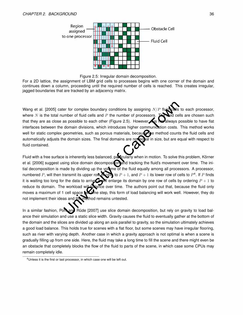
Univers

ity of

Cap

e Tow

n


Figure 2.5: Irregular domain decomposition.For a 2D lattice, the assignment of LBM grid cells to processes begins with one corner of the domain andcontinues down a column, proceeding until the required number of cells is reached. This creates irregular,jagged boundaries that are tracked by an adjacency matrix.

Wang et al. [2005] cater for complex boundary conditions by assigning N/P fluid cells to each processor,where N is the total number of fluid cells and P the number of processors. The fluid cells are chosen suchthat they are as close as possible to each other (Figure 2.5). However, it is not always possible to have flatinterfaces between the domain divisions, which introduces higher communication costs. This method workswell for static complex geometries, such as porous materials, because the method counts the fluid cells andautomatically adjusts the domain sizes. The final domains are not equal in size, but are equal with respect tofluid contained.

Fluid with a free surface is inherently less balanced, particularly when in motion. To solve this problem, Körneret al. [2006] suggest using slice domain decomposition and tracking the fluid’s movement over time. The ini-tial decomposition is made by dividing up the volume of the fluid equally among all processors. A processor,numbered P , will then transmit its upper row of cells to P + 1, and P + 1 its lower row of cells to P 4. If P findsit is waiting too long for the data to arrive, it will enlarge its domain by one row of cells by ordering P + 1 toreduce its domain. The workload will balance over time. The authors point out that, because the fluid onlymoves a maximum of 1 cell space per time step, this form of load balancing will work well. However, they donot implement their ideas and the method remains untested.

In a similar fashion, Pohl and Rüde [2007] use slice domain decomposition, but rely on gravity to load bal-ance their simulation and use a static slice width. Gravity causes the fluid to eventually gather at the bottom ofthe domain and the slices are divided up along an axis parallel to gravity, so the simulation ultimately achievesa good load balance. This holds true for scenes with a flat floor, but some scenes may have irregular flooring,such as river with varying depth. Another case in which a gravity approach is not optimal is when a scene isgradually filling up from one side. Here, the fluid may take a long time to fill the scene and there might even bean obstacle that completely blocks the flow of the fluid to parts of the scene, in which case some CPUs mayremain completely idle.

4Unless it is the first or last processor, in which case one will be left out.

Univers

ity of

Cap

e Tow

n


2.6.4 Technologies

A popular technology for the parallelization of a simulation is the Message Passing Interface (MPI) communi-cation protocol, which is specifically designed to aid programming of parallel systems. Essentially, MPI definesfunctions that allow the programmer to pass data from one process to another in a similar fashion to sock-ets, but simplifications have been made to hide the usual network specifics, and management logic has beenadded to control a fleet of processes. These may be run concurrently on the same or a number of differentCPUs. The key focus of the protocol is program scalability, allowing a MPI-based program to run on from oneto thousands of CPUs simultaneously and MPI focuses on portability/generality.

An alternative to MPI is OpenMP, which is a thread based parallel programming technique for shared mem-ory systems as opposed to the process based approach of MPI for distributed memory architectures. MPI,however, allows the use of shared memory (when available, to improve performance) instead of socket com-munication. Krawezik [2003] shows that OpenMP does not offer significant performance increases over MPIon shared memory systems. He compares MPI implementations of the NAS Benchmarks [Bailey et al., 1991]against various OpenMP implementations and finds that OpenMP does offer some improvements, but they donot necessarily warrant the use of the programming environment.

2.7 Using High Performance Computing

Our goal is to produce a system that is capable of producing highly detailed fluid in complex scenes. Fluidsimulations have two potential bottlenecks: the number of floating point operations (due to the use of physi-cal equations) and memory access (due to the large amount of data that needs to be simulated for detailedscenes). Both of these bottlenecks become exaggerated when one wants to produce a large scene with highquality. The time needed to run such a simulation on a single CPU is not practical. One may wish to distributethe simulation across a cluster or any computing resources available; this could be a number of clusters orpossibly even grid computing resource.

Special architectures have been developed to deal with the algorithms using of many floating point opera-tions and high memory bandwidth. One such technology is the Cell broadband engine architecture (CBE),which is a multi-core CPU. An example of an application is given in Sturmer et al. [2007]. The authors usethis architecture, running a LBM fluid simulation, to simulate 2 heartbeats in 11 minutes. They achieve up to 4times speed up over the same simulation software on a quad core XEON system running at 3Ghz.

Another attractive approach taken by a number of authors is the use of Graphics Processing Unit (GPU)acceleration. GPUs allow a very high degree of parallelism and can perform many floating point operations atthe same time. The newest graphics card from NVIDIA, the GTX 280, has a theoretical maximum performanceof 933GFlops. Wei et al. [2003] use a LBM on the GPU to simulate wind effects on objects such as feathersand bubbles. The use of the GPU gives a 9 times speed up over their CPU implementation. Li et al. [2003] alsoimplement LBM on the GPU with a speed up of 50, but comment on the reduced accuracy due to the singleprecision nature of GPUs. They produce animations of steam and smoke. Keenan Crane produced real-timefluid simulations at grid resolutions of 64x64x128 on the GPU using the popular stable fluids method (see Sec-tion 2.4.1.1) of Howes and Thomas [2007]. While there has been progress made and Fan et al. [2004] haveshown real time simulation of the underlying fluid dynamics, at the time of writing there is no known solution

Univers

ity of

Cap

e Tow

n


for realtime free surface flows on a GPU [Thuerey, 2008].

In feature films such as Poseidon, the fluid simulations are distributed across a group of 5 Networked LinuxPCs and run using an in-house software package, known as RealFlow 5. Unfortunately they do not report thetime taken for the simulations. On their benchmarking page, they report a simulation time of 30 mins for asimple breaking dam example on an AMD Opteron machine with 32 processors. This time frame is acceptablefor use in a production environment, but this is a simple scene. During the making of Surf’s Up, the breakingwaves were simulated overnight on a cluster to be available for animators the next morning. Due to the unpre-dictability of the simulations and the length of time for a single run, multiple initial conditions were run, so thatthe best one could be chosen the next morning [Carlson, 2007].

There has been wide adoption of the use of multi-core programming to speed up simulations. In an interview,Ron Fedkiw, of Industrial Light + Magic, said that the ability to adapt algorithms for simulations to multi-coreenvironments has been key to the high quality simulations we see in current movies. He also added that nowscene changes by the animators can be integrated quickly into the fluid simulations [Peszko, 2006]. In thefilm 300, a full battle scene on the ocean, where objects influence the water and not vice versa, is simulatedusing a cluster of about 80 PCs [Trojansky et al., 2007]. This allows for a very large scene as there is thecombined memory and processing power of all the PCs. However, the programming overhead is far higherand the network backbone becomes important. These issues will be further discussed in Chapter 5.

2.8 Conclusion

When considering a simulation system, one can mix and match many of the methods described here in anynumber of combinations. However, some may be more suitable for certain situations. Furthermore, certainsurface representations may combine better with a given dynamics simulation. It is important to choose thecorrect methods for a given application. In our case this is large scenes with high detail and dynamic objectsfor movies. To this end we choose the Lattice Boltzmann Method.

This uses a simple representation that handles dynamic boundary conditions well. The simplicity of the al-gorithm is important, as an efficient implementation will have fewer lines of code, be easier to debug andallows for more straightforward extensions. The VOF method applies well to the LBM, as movement of fluidmass is directly equal to the distribution functions, and will be used in our simulations as the chosen fluidsurface representation.

The LBM is not very well known in the graphics community, but is a promising avenue of research. Gelleret al. [2006] give a comparison of the efficiency comparison of the LBM and the traditional Finite-Elementmethod (a generalisation of the finite difference approach with similar characteristics). They conclude that theLBM is “at least as competitive” as the traditional method, but only for more turbulent cases. For films, ingeneral, we are only interested in turbulent cases, as the calm fluid cases are easily created by hand.

There are many approximations that reduce the computation time of fluid simulations, but these are mostlyat the cost of lower scene detail and less turbulence. We seek to preserve as much detail as possible. Assuch, we will aim to make used of high resolution grids. In order to make the simulation times practical, use of

5www.RealFlow.com

Univers

ity of

Cap

e Tow

n


HPC technology will be required. Parallel computing resources, such as a cluster, are used, as this gives usaccess to larger memory areas and high computation rates. Use of the GPU and CBE are also plausible, butdue to the high degree of branching required for the VOF representation, might not perform as well. The LBMis particularly suited to such parallel environments as only local information (neighbouring cells) is neededduring the update of a cell.

We investigate a LBM VOF implementation on a cluster architecture. An efficient solution is an interestingproblem to solve as parallel fluid simulation has become increasingly popular with the price of hardware perGHz continuing to drop over recent years. More and more animation companies own their own clusters to usefor computation tasks and have access to other similar resources. There are many centers around the worldand proper use of the resources will allow us to produce high quality simulations. For instance, the Centre forHigh Performance Computing in South Africa gives access to a cluster of 160 nodes, each with the two dualcore XEON’s and 17Gb memory.

Univers

ity of

Cap

e Tow

n

Chapter 3

LBM Fluid Simulation

One of our purposes in this thesis is to build a system that produces fluid for a 3D scene by modelling itsphysical characteristics. This chapter builds on information presented in Chapter 2 and describes, with moredetail, the physical quantities used to model the fluid and the underlying equations. It avoids a more formaldescription of the data structures used in the implementation and the details about the simulation of the fluidsurface. For that, the reader is referred to the subsequent chapter.

The chapter begins by providing a basic description of the Lattice Boltzmann Method (LBM) in 3D and thesteps required to use it to simulate fluid in Section 3.1. The Boltzmann equation is then introduced in Section3.2. This is the fundamental equation that drives the fluid behavior and from this the LBM is derived. From themodel, Section 3.2.2 then describes important details taken from the proof that the Navier-Stokes equations(see Section 2.3) can be recovered. As with all numerical simulations, the numerical stability is important andrequires discussion (Section 3.2.3).

3.1 Full Algorithm Description for 3D

To add fluid to a scene using the LBM, the scene is first divided up into a 3D grid. Each grid point or cell storesinformation about velocity, density and particle distribution functions of the fluid at a point in space. For themoment, we assume that there is no free surface, i.e. no division between fluid and air, and the whole sceneis completely filled with fluid. The particle distribution functions seek to simulate atomic interactions such asattraction and repulsions that occur within the fluid. These interactions are modelled with cellular automatarules that use physical equations to update grid cells. The rules describe how the particles move within thefluid, which is termed streaming, and also how they collide with one another.

A LBM grid is called a lattice, as it is a regular arrangement of squares (2D) or cuboids (3D). Figure 3.1gives the general structure of the D3D19 lattice. The name of the lattice comes from the 19 distribution func-tions (D19) stored for each grid position with each distribution function assigned to a particular velocity in threedimensions (D3). There are many popular variants of lattices for different dimensions: D2D9, D3D15 andD3D27 [Wei et al., 2004a]. Naturally, the simpler the lattice the faster the simulation.

40

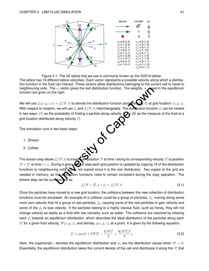
Univers

ity of

Cap

e Tow

n

CHAPTER 3. LBM FLUID SIMULATION 41

Figure 3.1: The 3D lattice that we use is commonly known as the D3D19 lattice.The lattice has 19 different lattice velocities. Each vector represents a possible velocity along which a distribu-tion function in the fluid can interact. These vectors allow distributions belonging to the current cell to travel toneighbouring cells. The c1 vector gives the rest distribution function. The weights, wi, used in the equilibriumfunction are given on the right.

We will use fi(x, y, z, t) = fi(−→x , t) to denote the distribution function along velocity −→ci at grid location (x, y, z).With respect to notation, we will use fi and fi(−→x , t) interchangeably. The distribution function fi can be viewedin two ways: (1) as the probability of finding a particle along velocity −→ci , or (2) as the measure of the fluid at agrid location distributed along velocity −→ci .

The simulation runs in two basic steps:

1. Stream

2. Collide

The stream step allows fi(−→x , t) to travel from position−→x at time t along its corresponding velocity−→ci to position−→x +−→ci at time t+ 1. During a given stream step each grid position is updated by copying 18 of the distributionfunctions to neighbouring cells. f0 is not copied since it is the rest distribution. Two copies of the grid areneeded in memory, as the distribution functions need to remain consistent during the copy operation. Thestream step can be summarised as

fi(−→x +−→ci , t+ 1) = fi(−→x , t) (3.1)

Once the particles have moved to a new grid location, the collisions between the new collection of distributionfunctions must be simulated. An example of a collision could be a group of particles, fk, moving along somenone zero velocity that hit a group of rest particles, f0, causing some of the rest particles to gain velocity andsome of the fk to lose velocity. If the particles belong to a highly viscous fluid, such as honey, they will notchange velocity as easily as a fluid with low viscosity, such as water. The collisions are resolved by relaxingeach fi towards an equilibrium distribution, which describes the ideal distribution of the particles along each−→ci for a given fluid velocity, −→u (x, y, z), and density, ρ(x, y, z), at a point. It is given by the following equation:

fei = ρwi[1 + 3−→u−→ci −3(−→u )2

2+

9(−→u−→ci )2

2]. (3.2)

Here, the superscript e denotes the equilibrium distribution and wi are the distribution values when −→u = 0.Essentially, the equilibrium distribution takes the current density of the cell and distributes it along the −→ci that

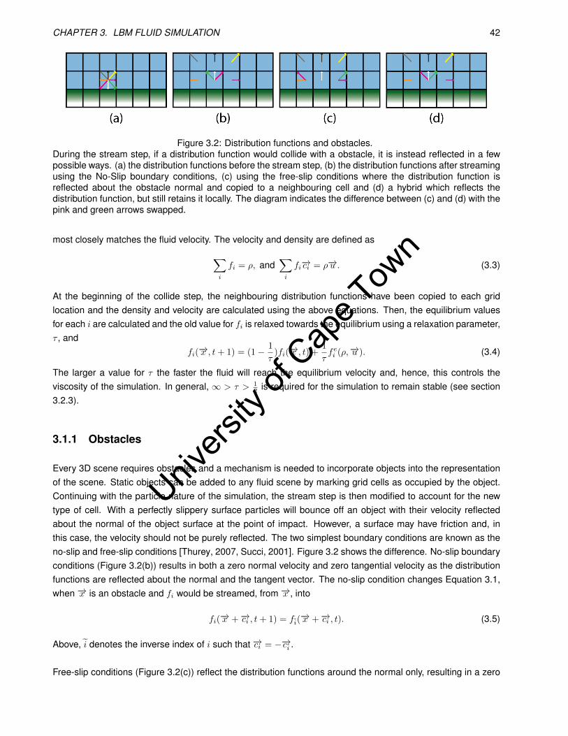
Univers

ity of

Cap

e Tow

n


Figure 3.2: Distribution functions and obstacles.During the stream step, if a distribution function would collide with a obstacle, it is instead reflected in a fewpossible ways. (a) the distribution functions before the stream step, (b) the distribution functions after streamingusing the No-Slip boundary conditions, (c) using the free-slip conditions where the distribution function isreflected about the obstacle normal and copied to a neighbouring cell and (d) a hybrid which reflects thedistribution function, but still retains it locally. The diagram indicates the difference between (c) and (d) with thepink and green arrows swapped.

most closely matches the fluid velocity. The velocity and density are defined as∑i

fi = ρ, and∑i

fi−→ci = ρ−→u . (3.3)

At the beginning of the collide step, the neighbouring distribution functions have been copied to each gridlocation and the density and velocity are calculated using the above equations. Then, the equilibrium valuesfor each i are calculated and the old value for fi is relaxed towards the equilibrium using a relaxation parameter,τ , and

fi(−→x , t+ 1) = (1− 1

τ)fi(−→x , t) +

1

τfei (ρ,−→u ). (3.4)

The larger a value for τ the faster the fluid will reach the equilibrium velocity and, hence, this controls theviscosity of the simulation. In general, ∞ > τ > 1

2 is required for the simulation to remain stable (see section3.2.3).

3.1.1 Obstacles

Every 3D scene requires obstacles and a mechanism is needed to incorporate objects into the representationof the scene. Static objects can be added to any fluid scene by marking grid cells as occupied by the object.Continuing with the particle nature of the simulation, the stream step is then modified to account for the newtype of cell. With a perfectly slippery surface particles will bounce off an object with their velocity reflectedabout the normal of the object surface at the point of impact. However, a surface may have friction and, inthis case, the velocity should not be purely reflected. The two simplest boundary conditions are known as theno-slip and free-slip conditions [Thurey, 2007, Succi, 2001]. Figure 3.2 shows the difference. No-slip boundaryconditions (Figure 3.2(b)) results in both a zero normal velocity and zero tangential velocity as the distributionfunctions are reflected about the normal and the tangent vector. The no-slip condition changes Equation 3.1,when −→x is an obstacle and fi would be streamed, from −→x , into

fi(−→x +−→ci , t+ 1) = fi(−→x +−→ci , t). (3.5)

Above, i denotes the inverse index of i such that −→ci = −−→ci .

Free-slip conditions (Figure 3.2(c)) reflect the distribution functions around the normal only, resulting in a zero

Univers

ity of

Cap

e Tow

n


normal velocity, but leaving the tangential velocity as is. This gives

fi(−→x +−→ci , t+ 1) = fr(−→x +−−→cFS , t).

Here, r is a new index, which gives the reflection vector of i and FS is a value to choose which neighbouringcell the distribution function should be fetched from. The disadvantage of free-slip conditions is that when anobstacle is found during streaming, extra neighbourhood look-ups are necessary. There are some tricky casesin corners when it is not obvious where the distribution function should be fetched from and a neighbourhoodsearch must be performed. This complicates the code and reduces efficiency, as the condition is no longera simple look-up table. It is also possible to combine the two previous conditions, so that, depending on theobstacle’s material, more or less slipping can occur [Thurey, 2007].

We use a simple hybrid of the two, shown as (d) in figure 3.2. Here, a colliding distribution function is reflectedabout the normal only and retained locally in the current cell. This allows the correct particle bounce-backbehaviour and the tangential velocity is no longer zero as with the no-slip conditions. Further, this all occurslocally, so no extra neighbour look-ups are necessary. We now have

fi(−→x +−→ci , t+ 1) = fr(−→x +−→ci , t). (3.6)

3.1.2 Gravity and external forces

Until now, gravity has been excluded from the model, but it is easily added during the collide step after thecalculation of the fluid velocity, by accelerating the velocity with the gravity constant. This is possible due to twoactions that are performed in the collide step. The first is the calculation of the aggregate cell velocity from thedistribution functions. This velocity is stored and used in the calculation of the new distribution functions for thenext time step. However, the velocity can be freely manipulated before the second action. If, for instance, therewas some reason to zero the velocity for some points in the grid, this would be possible here. Instead, thenatural action of adding the acceleration due to gravity is performed. Effectively, the new distribution functionscalculated are distributed towards the side of the cell that matches the gravity vector direction.

At this point, it is also possible to add control forces generated from an external source. Thürey et al. [2006]use control particles with attraction forces, to pull fluid towards certain positions, and velocity forces, to makethe fluid match certain velocities. This is performed on multiple scales to preserve small fluid details whileallowing control of overall fluid behaviour.

3.1.3 Simulation Initialisation

The model described so far has assumed that most values, such as the time step and space step, are correctlynormalised. In the real world the scene division will not be as straightforward. Hence, a translation is neededfrom the scene dimensions into the lattice dimensions. Following Thurey et al. [2005a], the initial values for thelattice are outlined here. The first parameter chosen is ∆x, the length of a grid cell. Since the lattice is a cube,there is only one length parameter. Once this has been chosen, the time step is selected to fulfill the stability

Univers

ity of

Cap

e Tow

n


conditions (see section 3.2.3), expressed as

∆t =

√gc∆x

|g|, (3.7)

where g is gravity and gc = 0.005 is a constant chosen to limit the time step to a small value to maintain stability.The kinematic viscosity, given in m2s−1, of the fluid is normalised to lattice units by

vlattice = vfluid∆t

(∆x)2. (3.8)

Gravity is also converted into lattice units as

glattice = gfluid(∆t)2

∆x. (3.9)

Lastly, the relaxation parameter τ is calculated as

τ = 3vlattice +1

2(3.10)

The individual distribution functions for each grid location are initialised using the equilibrium distribution witha given velocity, usually zero, in which case the distribution functions are set to the individual weights.

3.2 Physical Derivation

In the previous section the final LBM method was presented. However, to properly make use of the method, thephysical significance needs to be understood. This section provides a first principles derivation of the methodto show why it is a physically based method.

The desired output of our fluid simulation is a fluid surface. To move this we need to know the velocity ofthe fluid near the surface so that we can advect it for each time step. However, in order to achieve this, avelocity model of the entire fluid is required. The movement of a volume of fluid at the bottom of a containerwill cause a disturbance at the surface due to the attraction and repulsion forces between millions of nearbyparticles.

In section 2.4 two approaches to modelling the velocity, Eularian and Lagrangian, were described. The Eular-ian approach directly computes the macroscopic quantities for a give point in space, while the Lagrangian ap-proach places particles in space with fluid like inter-particle forces. In physics the eularian approach came firstin the form of the Navier-Stokes equations by Louis M. H. Navier (1785-1836) and Sir George Babriel Stokes(1819-1903) followed by the Lagrangian approach in the form of the Boltzmann equation [Wolf-Gladrow, 2000].

The LBM was created after many iterations of different lattice gas methods. It is possible to trace througheach of these steps to obtain the current algorithm, but a greater understanding of how the algorithm workscan be gained by its derivation from the physical equations. Here, the latter approach is taken, beginning witha grounding in some of the earlier work in physics.

The Boltzmann equation models the collisions of particles in a simplistic fashion, using three rules: (1) only two

Univers

ity of

Cap

e Tow

n


particles are present in a collision, (2) the velocities of the particles are linearly independent and (3) there areno external forces present during the collision. The equation does not consider individual particles, but rathera distribution of particles, f(−→x ,−→v , t), which is defined such that f(−→x ,−→v , t)d−→v d−→x is the number of particlesin a small portion of space, d−→x , travelling in a small range of velocities, d−→v [Bhatnagar et al., 1954]. Thedistribution f is also known as the probability distribution of the particles and the integral of f over the wholespace will yield the total number of particles. The time evolution of f for a given point, −→x , and velocity, −→v , isthen given by

∂f

∂t+−→v ∂f

∂−→x+−→g ∂f

∂−→v= Ω(f), (3.11)

where −→g is gravity and Ω is the collision operator. In short, the equation captures the change in the particledistribution due to the distribution’s spatial gradient at the position and velocity (the second term from the left),the acceleration of gravity (the third term) and lastly the inter-collisions of particles (the right hand side). Thecollision operator models all possible collisions between every pair of particles and is defined as

Ω(f) =

∫(f ′1f

′2 − f1f2)σ(|−→u1 −−→u2| , ω)d−→ω d−→p .

This integrates the change in the distribution function due to all particle collisions, which always involve only twoparticles by assumption, and is performed by integrating over −→p , the possible momentums of a single particle,and ω, the solid angle. This angle defines the velocity of the second particle, −→u2, relative to the first, −→u1 = −→p /m(m is the mass of a particle). For a given pair of velocities, −→u1 and −→u2, the probability of a collision occurring isgiven by the differential cross section operator, σ modelled by approximating the particles as spheres [Thürey,2003]. Now, once the probability of a collision is known, the change in the global distribution function f is thedifference in the distribution functions before the collision, f1f2, and after the collision, f ′1f ′2, calculated fromthe known particle velocities. The operator is included as it shows the complexity needed to model a particlesystem perfectly. For a more detail description the reader is referred to Succi [2001].

The main problem with the collision operator as it stands, is that it is very complex and computationally infea-sible to model. Bhatnagar et al. [1954] introduced a new collision operator by relaxing the current distributionto an equilibrium distribution, fe. This is performed using a collision time τ and the following equation,

Ω(f) =fe − fτ

.

The approximation uses the H-theorem, which shows that f will tend to a Maxwellian distribution, fe, to reachthe lowest potential energy for the system [Thürey, 2003]. The collision time, τ , controls how fast the dis-tribution will relax to equilibrium and fe can be derived at the point where collisions have no effect on thedistribution, i.e. Ω(fe, fe) = 0.

Up to this point, the equations that model the underlying micro-dynamics of a particle system have been pro-vided, but to measure the equilibrium of the system the macroscopic velocity, vm, and density, ρ, are required.These, respectively, are an aggregation of the particle behaviour given by f as

ρ(−→x ) =

∫fd−→v , and (3.12)

Univers

ity of

Cap

e Tow

n


−→vm(−→x ) =

∫ −→v fd−→vρ(−→x )

. (3.13)

The mass of the particle is normalized to unity in these equations. Now, with the macroscopic velocity anddensity, the equilibrium particle distribution at −→x is

g(−→vm) = fe(−→v ,−→x ,−→vm) =ρo

2π(RT )D/2e−

(v−vm(−→x ))2

2RT , (3.14)

where ρo is the reference density (usually 1), R is the Ideal Gas Constant, D is the number of dimensions andT is the fluid temperature. This distributes the particles along velocities that agree most with the macroscopicvelocity.

The Boltzmann equation gives us a link from the micro dynamics of particle interactions to the macro dy-namics of fluid behaviour. The LBM uses this as a basis for fluid simulation. Using these tools, in the nextsection we will derive the LBM from the Boltzmann equation.

3.2.1 Lattice Boltzmann Method

The LBM is obtained by a special discretization of equation 3.11. Here, a derivation is presented. This is notas complete as texts such as Succi [2001] or Wolf-Gladrow [2000], but provides a correct derivation that is assimple as possible. The fluid space will be divided up into a grid, which allows the particle distributions to betracked over time.

A finite set of velocities, −→ci , is introduced as the velocities along which particles will be allowed to travel.For each of these velocities, a corresponding discrete function, fi(−→x ,−→ci , t), is defined and Equation 3.11 withthe simplified collision operator is now:1

∂fi∂t

+−→ci∂fi∂−→x

=fei − fiτ

. (3.15)

The equation is further discretized with respect to time and space:

fi(−→x , t+ ∆t)− fi(x, t)∆t

+ cixfi(−→x + ∆x, t+ ∆t)− fi(−→x , t+ ∆t)

∆x+

ciyfi(−→x + ∆y, t+ ∆t)− fi(−→x , t+ ∆t)

∆y+

cizfi(−→x + ∆z, t+ ∆t)− fi(−→x , t+ ∆t)

∆z=

fei − fi(−→x , t)τ

(3.16)

As ∆t and ∆x in the discretization are arbitrary, ∆x = ∆y = ∆z = ∆t is chosen. Substituting the 3 spatialdifferential terms on the left with an approximation of the discretized components into one term2, leads to

fi(−→x , t+ ∆t)− fi(x, t)∆t

+fi(−→x +−→ci∆t, t+ ∆t)− fi(−→x , t+ ∆t)

∆t=fei − fi(−→x , t)

τ. (3.17)

1the gravity term has been excluded for simplicity and is not required, see section 3.1.22Instead of sampling f with individual steps along each of the axes and weighting the differences with the ciα, f is sampled at the full

step along −→ci .

Univers

ity of

Cap

e Tow

n


The last substitution we make is τ = τ∆t and we multiply by ∆t to get what is called the Lattice Boltzmann

Equation (LBE):

fi(−→x + ci∆t, t+ ∆t)− fi(−→x , t) =fei − fi(−→x , t)

τ. (3.18)

However, the equilibrium function, fei , has not yet been defined. First, equation 3.14 needs to be trans-formed into a different form, which is obtained by the third order Taylor expansion of g(−→vm). Let cs =

√RT

and β = ρ(2πc2s)D/2 e

− (−→v )2

2c2s then g(−→vm) = βe− (−→vm)2

2c2s+−→vm−→v

c2s . The important derivatives are then ∇g(−→vm) =

βe− (−→vm)2


c2s [−−→vmc2s

+−→vc2s

], gxx(−→vm) = βc2se− (−→vm)2


c2s [−1 + (vmx+vx)2

c2s], gyy(−→vm) = β

c2se− (−→vm)2


c2s [−1 +

(vmy+vy)2

c2s] and gxy(−→vm) = β

c2se− (−→vm)2


c2s [(vx−vmx)(vy−vmy)

c2s]. By the chain rule and differentiability of the

exponential function, g is differentiable everywhere and the Taylor expansion around −→0 3 up to second order is

g(−→vm) = g(0) +−→vm · ∇g(−→vm) +1

2(v2mxgxx(

−→0 ) + vmxvmygxy(

−→0 ) + v2

mygyy(−→0 )) +O(∂3g(−→vm))

= β[1 +−→vm−→vc2s

+1

2c2s(v2mxv

2x

c2s− v2

mx + 2vmxvmyvxvy +v2myv

2y

c2s− v2

my)]

=ρ

(2πc2s)D/2

e− (−→v )2

2c2s [1 +−→vm−→vc2s− (−→vm)2

2c2s+

(−→vm−→v )2

2c4s]

As each of our velocities will be discrete and the leading exponential will be constant, the simplified MaxwellianDistribution is

fei (−→vm) = ρwi[1 +−→vm−→vc2s− (−→vm)2

2c2s+

(−→vm−→v )2

2c4s]. (3.19)

The weight, wi, is included to ensure that the new discrete distribution agrees with the continuous one forzero velocities. The simulations considered in this thesis are isothermal and, hence, cs becomes an arbitraryconstant [He and Luo, 1997].

When −→v or −→vm are zero we have a new discrete distribution given by wi. To ensure the consistency of thisdistribution, the concept of moments is introduced. The moments of a distribution function, f , around zeroare defined as

∫∞−∞ xnf(x)dx, where n denotes the nth-moment. For n = 1 the moment is just 1, for n = 2

the moment is the expected value of the distribution, for n = 3 the moment is a measure of the skewnessof f and for forth moment it measures whether f is tall, skinny or squat. The moments of equation 3.14 arecalculated using coordinate-wise Gaussian integrals while the discrete version given by wi is a straightforwardsummation. The moments up to the fourth order are equated as below (from [Wolf-Gladrow, 2000]),

∑i

wi =

∫g(−→vm)d−→vm = 1 (3.20)

∑i

wiciα =

∫vmαg(−→vm)d−→vm = 0 (3.21)

∑i

wiciαciβ =

∫vmαvmβg(−→vm)d−→vm = poc

2sδαβ (3.22)

∑i

wiciαciβciγ =

∫vmαvmβvmγg(−→vm)d−→vm = 0 (3.23)

∑i

wiciαciβciγciθ =

∫vmαvmβvmγvmθg(−→vm)d−→vm = p0c

4s(δαβδγθ + δαγδβθ + δαβδβγ) (3.24)

3−→0 = (0, 0)

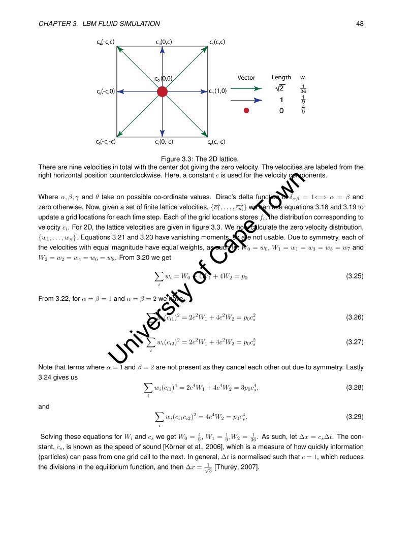
Univers

ity of

Cap

e Tow

n


Figure 3.3: The 2D lattice.There are nine velocities in total with the center dot giving the zero velocity. The velocities are labeled from theright horizontal position counterclockwise. Here, a constant c is used for the velocity components.

Where α, β, γ and θ take on possible co-ordinate values. Dirac’s delta function is δαβ = 1⇐⇒ α = β andzero otherwise. Now, given a set of finite lattice velocities, −→c1 , . . . ,−→cn, we can use equations 3.18 and 3.19 toupdate a grid locations for each time step. Each of the grid locations stores fi, the distribution corresponding tovelocity ci. For 2D, the lattice velocities are given in figure 3.3. We now calculate the zero velocity distribution,w1, . . . , wn. Equations 3.21 and 3.23 have vanishing moments, so are not usable. Due to symmetry, each ofthe velocities with equal magnitude have equal weights, as such let W0 = w0, W1 = w1 = w3 = w5 = w7 andW2 = w2 = w4 = w6 = w8. From 3.20 we get∑

i

wi = W0 + 4W1 + 4W2 = p0 (3.25)

From 3.22, for α = β = 1 and α = β = 2 we have∑i

wi(ci1)2 = 2c2W1 + 4c2W2 = p0c2s (3.26)

∑i

wi(ci2)2 = 2c2W1 + 4c2W2 = p0c2s (3.27)

Note that terms where α = 1 and β = 2 are not present as they cancel each other out due to symmetry. Lastly3.24 gives us ∑

i

wi(ci1)4 = 2c4W1 + 4c4W2 = 3p0c4s, (3.28)

and ∑i

wi(ci1ci2)2 = 4c4W2 = p0c4s. (3.29)

Solving these equations for Wi and cs we get W0 = 49 , W1 = 1

9 ,W2 = 136 . As such, let ∆x = cs∆t. The con-

stant, cs, is known as the speed of sound [Körner et al., 2006], which is a measure of how quickly information(particles) can pass from one grid cell to the next. In general, ∆t is normalised such that c = 1, which reducesthe divisions in the equilibrium function, and then ∆x = 1√

3[Thurey, 2007].

Univers

ity of

Cap

e Tow

n


For the 2D lattice the velocity and density for a given grid point are calculated as:

8∑i=0

fi = ρ (3.30)

8∑i=0

−→ci fi = ρ−→u (3.31)

The LBM for two dimensions is defined by the choice of −→ci and the derived wi. These are chosen with sufficientsymmetry to allow the recovery of Navier-Stokes.

3.2.2 Proof of physical correctness

The full proof of correctness is too lengthy and detailed to present here. Instead, it has been included inAppendix B. In essence, the proof rests on the assumption that fluid and particle behaviour can be analysedon different scales. The distribution functions are decomposed into such different scales. The Taylor expansionof the LBE equation and the translations from the distribution functions to the macroscopic values of pressureand velocity in Equation 3.3 are then used to recover the Navier-Stokes equations. The most important resultfrom the proof is the relation between the relaxation parameter, τ , and the viscosity of the fluid given by

v =c2s∆t

3

(τ − 1

2

). (3.32)

In the equation, cs = ∆x∆t . In a normalised lattice with ∆t = ∆x = 1, this is

v =1

3(τ − 1

2). (3.33)

3.2.3 Numerical Stability

In general, there has been little concrete research into on the stability of the LBM. The most thorough descrip-tion of the topic can be found in Succi [2001]. The LBM is an explicit time-marching numerical scheme for thesolution of the Navier-Stokes equations. Time-marching is used to describe a method that takes finite steps intime to solve a partial differential equation. Explicit refers to the information required to take a step forward intime. Specifically, only information from the previous time step is required.

A common condition when using such a scheme is known as the Courant-Friedrichs-Lewy (CFL) condition[Körner et al., 2006]. The basic premise is that the information at a point in a discretized structure cannot travelfurther then the neighbouring points in one time step. A simple example of such an inconsistency is a particlewith velocity 2ms−1 traveling through a discrete grid with spacing of 1ms−1 and using a time step of 1sec. Now,the particle will move two grid spaces in one step and will not be able to take into account information, say acollision, in the space between its start and end position. In the case of the LBM this condition is

vmax <∆x

∆t= cs. (3.34)

This says that the maximum velocity, vmax, must be less then cs, the speed of sound of the lattice. Afternormalisation, ∆t = 1,∆x = 1√

3, the expression becomes |vmax| < 1√

3. A similar relation suggested by Thürey

Univers

ity of

Cap

e Tow

n


[2003] is obtained for gravity,g(∆t)2

∆x< 10−4. (3.35)

Here, the acceleration due to gravity is controlled. For our simulations this will be the only external force andthe time-step and space-step must be chosen to ensure that the velocity of the fluid is not accelerated fasterthen the maximum velocity for the lattice.

Further analysis of the stability can be performed by studying the conservation of various physical quanti-ties. The first being the viscosity of the fluid. This should never be negative and, hence, the restriction τ > 0.5

is derived from Equation 3.33. The other quantities that should not be negative are the distributions and sincethey are further restricted from above, 0 < fi, f

ei < 1 is obtained. Considering this and the equilibrium function

we can see that |vmax| < 23 . Succi [2001] use these same restrictions to derive the constraint u

2

2 + τux <13 .

This, however, is for a simplified 1 dimensional lattice, but does show that high speeds and a high velocitygradient will cause instabilities. They go one step further to suggest the relation 0.5 < h(−→u ) < τ where h issome function of the current velocity that limits the value of τ . It is not yet known what the value of h(−→u ) is.Essentially, τ can approach 0.5, but cannot get arbitrarily close. Thurey [2007] use a cut off value of 0.51,obtained from experimental procedures.

Muders [1995] find this gradient to be a cause of “spurious instabilities.” To combat this he introduces aparameter that increases the viscosity artificially in regions with velocities above a given threshold. He claimsthat this allows him to simulate fluids with speeds close to the speed of sound. In addition, he also usesa modified distribution function that takes into account a fourth order expansion of the Maxwellian distribution(in section 3.2 only order two was used). This modification uses 18 distinct equilibrium weights instead of our 3.

Another approach to increase the stability of the LBM is the Multiple-relaxation time method [d’Humières et al.,2002]. This method no longer uses the simplified relaxation operator of Bhatnagar et al. [1954], instead theyuse multiple relaxation times. This relaxes all the distribution functions at the same time. The collision operatorbecomes a function of all distribution functions instead of just the one previous distribution function and theequilibrium value. This moves the LBM towards an implicit method, relying on neighbouring distribution func-tion values, increasing the stability at the expense of a more complex method.

Hou et al. [1994] claim that numerical instability in the LBM is caused by unresolved fluid motion at scalesfiner then the chosen LBM grid. They introduce a damping term for the effects created by sub grid motion,stopping the motion from causing unwanted instabilities. The damping term uses Smagorinsky’s sub-gridmodel, also used in Thurey [2007] and Wei et al. [2003], which uses the local stress tensor as a measure ofthe sub grid turbulence at a point. For the LBM this is given by

∏α,β =

19∑i=1

ciαciβ(fi − fei ). (3.36)

Then the intensity of the local strain is calculated as

S =1

6C2

(√v2 + 18C2

√∏α,β

∏α,β − v

). (3.37)

Univers

ity of

Cap

e Tow

n


Here, C is the Smagorinsky constant, usually given a value in the range 0.2 − 0.4 and v is the viscosity. Therelaxation parameter is then modified to

τs = 3(v + C2S) +1

2. (3.38)

In effect this equation also artificially increases the viscosity of the simulation for points on the grid where thereis higher sub-grid turbulence, damping the effects of the turbulence.

To summarise, there are two main points of instability: (a) when the fluid moves faster then some vmax and (b)when the velocity gradient is too large for the LBM to handle. These have been controlled by Thurey [2007]using adaptive time steps and the Smagorinsky model. We adopt the second approach, but not the first. Highfluid speeds can be adequately dealt with by using sufficiently small time steps during the simulation, withoutadded complexity overhead.

3.3 Conclusion

This chapter has introduced the LBM and the fundamental link to the atomic interactions via the Boltzmannequation and the discrete distribution functions on a lattice. The interactions with obstacles were also de-fined using a slightly modified no-slip condition. The evolution of the distribution functions was defined by thestreaming and collision operators. The collision operator makes use of the Maxwellian distribution to correctlydistribute the particle probabilities within a lattice cell for each time step. Through the use of a relaxation pa-rameter, τ , the viscosity of the fluid can be controlled.

Lastly, the stability conditions for the LBM were discussed. Specifically, it is important to keep the spatialstep over time step ratio greater then the maximum velocity (see Equation 3.34) and to limit the time stepagainst gravity. To aid simulation stability, the Smagorinsky sub grid model was introduced.

Univers

ity of

Cap

e Tow

n

Chapter 4

Single CPU Implementation

We aim to generate 3D free-surface fluid simulations for movies, integrating the simulation into the popular 3Danimation package Houdini1. This will give an animator the ability to define a 3D scene and place fluid withinit. The fluid will be simulated using the underlying Lattice Boltzmann numerical method, presented in Chapter3. We now explore the fluid surface representation and how the fluid is embedded into the scene, beginningwith an algorithm overview in Section 4.1, followed by the mass tracking or Volume of Fluid (VOF) method inSection 4.2.

The VOF provides a voxel representation for the presence of fluid in the scene and can be rendered usingthree dimensional texture techniques, but, for fluids such as water, it is preferable to have a polygonal sur-face that can be input to a renderer to produce effects such as refraction and reflection. The marching cubesmethods is used to reconstruct a triangle surface from the VOF grid and is discussed in Section 4.3. Theintegration of the simulation into Houdini is discussed in Section 4.4. Lastly, the results from the single CPUfluid simulation and conclusions are presented in Sections 4.5 and 4.6.

4.1 Algorithm Summary

An overview of the VOF LBM algorithm appears in Figure 4.1. The LBM algorithm uses a voxel grid structureto simulate fluid in 3D during stream and collide (steps (1) and (2) in the figure), giving us the movement of thefluid for each position in the scene. To further track the movement precisely, we make use of the VOF methodto track which grid cells contain fluid.

Each grid location, in Figure 4.1, shows the fluid region divided into four states: fluid, interface, empty andobstacle cells. The fluid cells represent cells that are completely filled with fluid and conversely empty cellsare completely without fluid. Interface cells form the boundary between filled and empty cells and are partiallyfilled. A filled cell must be surrounded only by fluid and interface cells, as fluid moves through the grid by ex-changing mass with non-empty cells. This mass exchange is implemented in parallel using the stream step forefficiency. The Process Queues step is added to manage the filling and emptying of cells (step (3) in the figure).

1www.sidefx.com

52

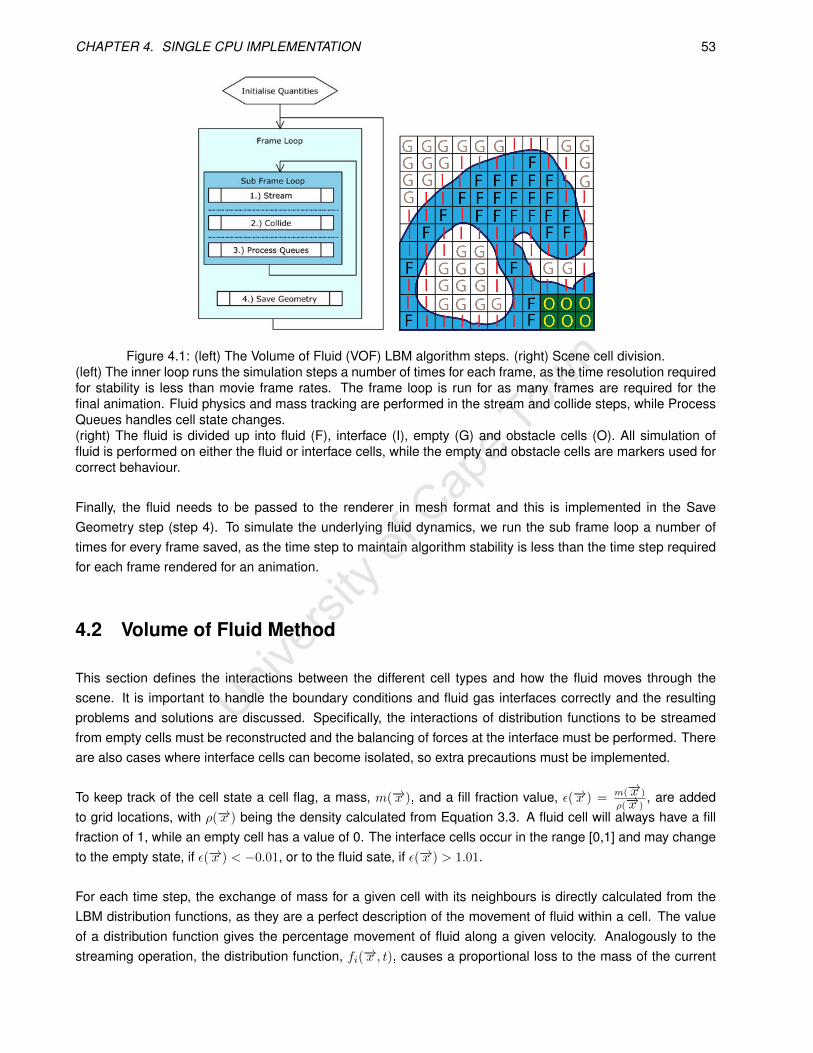
Univers

ity of

Cap

e Tow

n

CHAPTER 4. SINGLE CPU IMPLEMENTATION 53

Figure 4.1: (left) The Volume of Fluid (VOF) LBM algorithm steps. (right) Scene cell division.(left) The inner loop runs the simulation steps a number of times for each frame, as the time resolution requiredfor stability is less than movie frame rates. The frame loop is run for as many frames are required for thefinal animation. Fluid physics and mass tracking are performed in the stream and collide steps, while ProcessQueues handles cell state changes.(right) The fluid is divided up into fluid (F), interface (I), empty (G) and obstacle cells (O). All simulation offluid is performed on either the fluid or interface cells, while the empty and obstacle cells are markers used forcorrect behaviour.

Finally, the fluid needs to be passed to the renderer in mesh format and this is implemented in the SaveGeometry step (step 4). To simulate the underlying fluid dynamics, we run the sub frame loop a number oftimes for every frame saved, as the time step to maintain algorithm stability is less than the time step requiredfor each frame rendered for an animation.

4.2 Volume of Fluid Method

This section defines the interactions between the different cell types and how the fluid moves through thescene. It is important to handle the boundary conditions and fluid gas interfaces correctly and the resultingproblems and solutions are discussed. Specifically, the interactions of distribution functions to be streamedfrom empty cells must be reconstructed and the balancing of forces at the interface must be performed. Thereare also cases where interface cells can become isolated, so extra precautions must be implemented.

To keep track of the cell state a cell flag, a mass, m(−→x ), and a fill fraction value, ε(−→x ) = m(−→x )

ρ(−→x ), are added

to grid locations, with ρ(−→x ) being the density calculated from Equation 3.3. A fluid cell will always have a fillfraction of 1, while an empty cell has a value of 0. The interface cells occur in the range [0,1] and may changeto the empty state, if ε(−→x ) < −0.01, or to the fluid sate, if ε(−→x ) > 1.01.

For each time step, the exchange of mass for a given cell with its neighbours is directly calculated from theLBM distribution functions, as they are a perfect description of the movement of fluid within a cell. The valueof a distribution function gives the percentage movement of fluid along a given velocity. Analogously to thestreaming operation, the distribution function, fi(−→x , t), causes a proportional loss to the mass of the current

Univers

ity of

Cap

e Tow

n


cell, while an adjacent inverse distribution function, fi(−→x +−→ci , t), causes a gain in mass. The change in massalong velocity i can then be computed as

∆mi(−→x , t) = fi(−→x +−→ci , t)− fi(−→x , t). (4.1)

For fluid cells the streaming operation applies unchanged, as the distribution functions already travel to neigh-bouring cells and fluid cells only share full boundaries with neighbouring fluid and interface cells. Interfacecells on the other hand are partially filled and the mass exchange is proportional to the shared area with otherinterface cells, which can be approximated by the corresponding fill fraction average of the two cells [Thureyet al., 2005a]. The interface-interface cell mass exchange is given as

∆mi(−→x , t) = (fi(−→x +−→ci , t)− fi(−→x , t))

(ε(−→x +−→ci , t) + ε(−→x , t))2

. (4.2)

It is only necessary to track the change of mass of fluid cells using Equation 4.1 and the interface-fluid cellsusing Equation 4.2. Combining all the changes for all velocities produces

m(−→x , t+ 1) = m(−→x , t) +19∑i=1

∆mi(−→x , t). (4.3)

In order to conserve mass, the mass exchange must be symmetric and the equations must be defined as such.This makes it necessary to store both fluid fraction and mass for each cell. The mass is updated during thestream step, while the fluid fractions are kept constant until after the mass exchange of all cells and then theupdated density is obtained from the collision step.

Empty cells have no relevant physical quantities, besides air pressure. During streaming, interface cells thatneighbour empty cells will not be able to copy the relevant distribution function, as it is undefined. In thesesituations, the distribution function is reconstructed and the streaming step (Equation 3.1) becomes

fi(−→x +−→ci , t+ 1) = fei (PA,−→u ) + fei(PA,−→u )− fi(−→x +−→ci , t). (4.4)

PA is the pressure of the air; usually a reference air pressure of 1 is employed. Using Boyle’s law we cantranslate the ideal gas pressure into density, which are the same in a normalised volume, V = 1.

In cases where an interface cell is surrounded by a small number of empty cells, only a few of the distri-bution functions will be reconstructed, causing unequal forces on the surface boundaries. We follow Thureyet al. [2005a], who reconstruct all fi that are in angular proximity to the surface normal. This is where the abso-

lute value of the angle between the normal for the current cell, −→n (−→x ) = 12 ×

ε(x− 1, y, z)− ε(x+ 1, y, z)

ε(x, y − 1, z)− ε(x, y + 1, z)

ε(x, y, z − 1)− ε(x, y, z + 1)

,

and the discrete velocity, −→ci , is less then π2 . Otherwise stated,

−→n (−→x ) · −→ci > 0. (4.5)

The surface normal is approximated from the fluid fill fraction discrete gradient. After these reconstructions,the distribution functions will be smooth along the surface edges and all cells will have valid values for thestreaming phases.

Univers

ity of

Cap

e Tow

n


After streaming is complete, during the collide step, the fill fraction of interface cells are checked to see whetherthey have crossed the thresholds for emptying or filling and, if so, the cell is added to a filled or emptied queue.The state is not changed immediately, as this would prevent the fluid state from remaining constant duringan entire update step. Instead, the Process Queues step is added as a post simulation step to handle statechanges.

The Process Queues step needs to correctly remove and initialise new interface cells. To maintain a layerof interface cells surrounding the fluid cells, the filled queue is processed and surrounding empty cells areconverted to interface cells. It is possible that one of the surrounding interface cells may be present in theemptied queue and must be removed, otherwise flickering of cell state will occur. Searching through the emp-tied queue for neighbouring cells is an expensive operation, so we introduce a queue position variable for eachgrid location. This increases the memory required for each cell by 2% (see Table 4.2 in Section 4.5). Theposition is initialised to -1 and when a cell is added to the emptied queue, its position in the queue is stored.Now, a check of whether a cell at a given position is in the emptied queue can now be performed in constanttime, at the cost of more memory consumption. Next, the resulting emptied queue is processed and any fluidcell adjacent to a cell being emptied is converted to an interface cell.

Empty cells that are converted into interface cells need valid values for pressure, velocity and distributionfunctions. The average of neighbouring non-empty cell values are used to obtain estimates of the velocity andpressure, as cells will have locally similar physical characteristics. The distribution functions are then initialisedusing the equilibrium distribution at the average pressure and velocity. Fluid cells converted to interface cellsretain their values, as the quantities are physically correct.

During conversion, the excess or negative excess mass, mex, above or below the thresholds is redistributed toneighbouring cells. For emptied cells, mex = m(−→x ) < 0, while for filled cells mex = ρ−m(−→x ). The redistribu-tion strategy is important, as the direction of the distribution will be visible as fluid movement. The excess massis shared amongst cells in the region of the interface normal [Thurey et al., 2005a], which is an approximationof the fluid movement direction, and weighted by the closeness of the normal and the direction towards theneighbouring cell, using

m(−→x +−→ci ) = m(−→x +−→ci ) +mex ·vi

vtotal, (4.6)

where for filled cells,

vi =

−→n · −→ci , if−→n · −→ci > 0;0, otherwise;

(4.7)

and for emptied cells,

vi =

−−→n · −→ci , if−→n · −→ci < 0;0, otherwise;

(4.8)

while vtotal =∑vi. The result of this operation is that the fluid surface is advected against to the normal for

emptied cells and with the normal for filled cells.

A drawback to this VOF implementation is that the fluid only moves in and out of interface cells and the surfacemotion is equivalent to the creation and removal of these cells. Should an interface cell have no neighbours,it will be unable to move. Thus, there may be small static pieces of fluid left, isolated in the grid. For fluidmovement to occur there must be two adjacent cells, so sheets or drops of water smaller than 2 grid cellscannot be simulated. To reduce these lone cells, Thurey et al. [2005a] try to enforce a single layer of interface

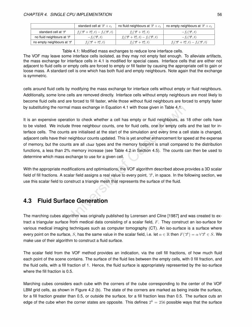
Univers

ity of

Cap

e Tow

n


standard cell at −→x + ci no fluid neighbours at −→x + ci no empty neighbours at −→x + ci

standard cell at −→x fi(−→x +−→ci , t)− fi(−→x , t) fi(

−→x +−→ci , t) −fi(−→x , t)

no fluid neighbours at −→x −fi(−→x , t) fi(−→x +−→ci , t)− fi(−→x , t) −fi(−→x , t)

no empty neighbours at −→x fi(−→x +−→ci , t) fi(

−→x +−→ci , t) fi(−→x +−→ci , t)− fi(−→x , t)

Table 4.1: Modified mass exchanges to reduce lone interface cells.The VOF may leave some interface cells isolated, as they may not empty fast enough. To alleviate artifacts,the mass exchange for interface cells in 4.1 is modified for special cases. Interface cells that are either notadjacent to fluid cells or empty cells are forced to empty or fill faster by causing the appropriate cell to gain orloose mass. A standard cell is one which has both fluid and empty neighbours. Note again that the exchangeis symmetric.

cells around fluid cells by modifying the mass exchange for interface cells without empty or fluid neighbours.Additionally, some lone cells are removed directly. Interface cells without empty neighbours are most likely tobecome fluid cells and are forced to fill faster, while those without fluid neighbours are forced to empty fasterby substituting the normal mass exchange in Equation 4.1 with those given in Table 4.1.

It is an expensive operation to check whether a cell has empty or fluid neighbours, as 18 other cells haveto be visited. We include three neighbour counts, one for fluid cells, one for empty cells and the last for in-terface cells. The counts are initialised at the start of the simulation and every time a cell state is changed,adjacent cells have their neighbour counts updated. This is yet another enhancement for speed at the expenseof memory, but the counts are all char types and the memory footprint is small compared to the distributionfunctions, a less than 2% memory increase (see Table 4.2 in Section 4.5). The counts can then be used todetermine which mass exchange to use for a given cell.

With the appropriate modifications and optimisations, the VOF algorithm described above provides a 3D scalarfield of fill fractions. A scalar field assigns a real value to every point, −→x , in space. In the following section, weuse this scalar field to construct a triangle mesh that represents the surface of the fluid.

4.3 Fluid Surface Generation

The marching cubes algorithm was originally published by Lorensen and Cline [1987] and was created to ex-tract a triangular surface from medical data consisting of a scalar field, F . They construct an iso-surface forvarious medical imaging techniques such as computer tomography (CT). An iso-surface is a surface whereevery point on the surface, S, has the same value in the scalar field, i.e. let α ∈ R then F (−→x ) = α ∀−→x ∈ S. Wemake use of their algorithm to construct a fluid surface.

The scalar field from the VOF method provides an indication, via the cell fill fractions, of how much fluideach point of the scene contains. The surface of the fluid lies between the empty cells, with 0 fill fraction, andthe fluid cells, with a fill fraction of 1. Hence, the fluid surface is appropriately represented by the iso-surfacewhere the fill fraction is 0.5.

Marching cubes considers each cube with the corners of the cube corresponding to the center of the VOFLBM grid cells, as shown in Figure 4.2 (b). The state of the corners are marked as being inside the surface,for a fill fraction greater than 0.5, or outside the surface, for a fill fraction less than 0.5. The surface cuts anedge of the cube when the corner states are opposite. This defines 28 = 256 possible ways that the surface

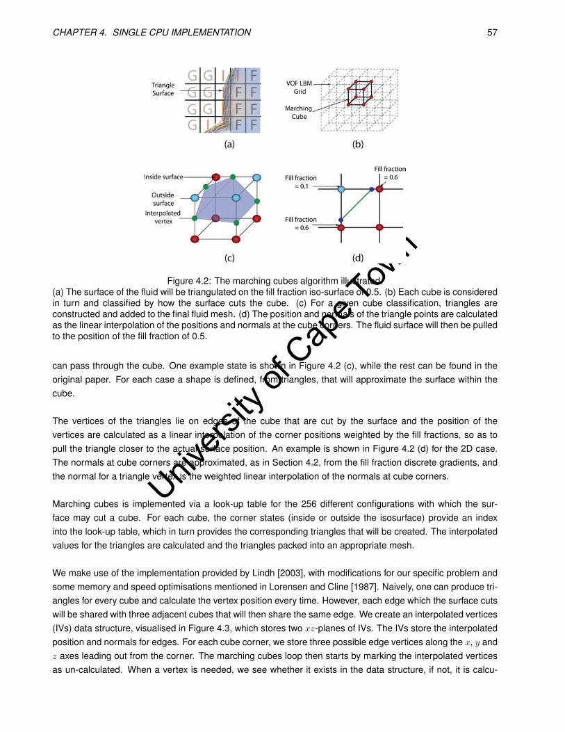
Univers

ity of

Cap

e Tow

n


Figure 4.2: The marching cubes algorithm illustrated.(a) The surface of the fluid will be triangulated on the fill fraction iso-surface of 0.5. (b) Each cube is consideredin turn and classified by how the surface cuts the cube. (c) For a given cube classification, triangles areconstructed and added to the final fluid mesh. (d) The position and normals of the triangle points are calculatedas the linear interpolation of the positions and normals at the cube corners. The fluid surface will then be pulledto the position of the fill fraction of 0.5.

can pass through the cube. One example state is shown in Figure 4.2 (c), while the rest can be found in theoriginal paper. For each case a shape is defined, from triangles, that will approximate the surface within thecube.

The vertices of the triangles lie on edges of the cube that are cut by the surface and the position of thevertices are calculated as a linear interpolation of the corner positions weighted by the fill fractions, so as topull the triangle closer to the actual surface position. An example is shown in Figure 4.2 (d) for the 2D case.The normals at cube corners are approximated, as in Section 4.2, from the fill fraction discrete gradients, andthe normal for a triangle vertex is the weighted linear interpolation of the normals at cube corners.

Marching cubes is implemented via a look-up table for the 256 different configurations with which the sur-face may cut a cube. For each cube, the corner states (inside or outside the isosurface) provide an indexinto the look-up table, which in turn provides the corresponding triangles that will be created. The interpolatedvalues for the triangles are calculated and the triangles packed into an appropriate mesh.

We make use of the implementation provided by Lindh [2003], with modifications for our specific problem andsome memory and speed optimisations mentioned in Lorensen and Cline [1987]. Naively, one can produce tri-angles for every cube and calculate the vertex position every time. However, each edge which the surface cutswill be shared with three adjacent cubes that will then share the same edge. We create an interpolated vertices(IVs) data structure, visualised in Figure 4.3, which stores two xz-planes of IVs. The IVs store the interpolatedposition and normals for edges. For each cube corner, we store three possible edge vertices along the x, y andz axes leading out from the corner. The marching cubes loop then starts by marking the interpolated verticesas un-calculated. When a vertex is needed, we see whether it exists in the data structure, if not, it is calcu-

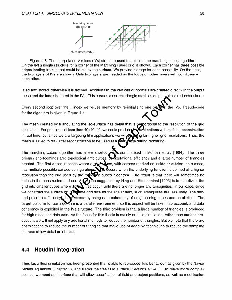
Univers

ity of

Cap

e Tow

n


Marching cubes

grid location

Interpolated vertex

Figure 4.3: The Interpolated Vertices (IVs) structure used to optimise the marching cubes algorithm.On the left a single structure for a corner of the Marching cubes grid is shown. Each corner has three possibleedges leading from it, that could be cut by the surface. We provide storage for each possibility. On the right,the two layers of IVs are shown. Only two layers are needed as the loops on other layers will not influenceeach other.

lated and stored, otherwise it is fetched. Additionally, the vertices or normals are created directly in the outputmesh and the index is stored in the IVs. This creates a correct triangle mesh as output with no redundant items

Every second loop over the z index we re-use memory by re-initialising one plane of the IVs. Pseudocodefor the algorithm is given in Figure 4.4.

The mesh created by triangulating the iso-surface has detail that is proportional to the resolution of the gridsimulation. For grid-sizes of less then 40x40x40, we could produce fluid animations with surface reconstructionin real time, but since we are targeting film applications we will be using far higher grid resolutions. Thus, themesh is saved to disk after reconstruction to be used at a later stage during rendering.

The marching cubes algorithm has a few shortcomings, summarised in Montani et al. [1994]. The threeprimary shortcomings are: topological ambiguities, computational efficiency and a large number of trianglescreated. The first arises in cases where a given cube, with corners marked as inside or outside the surface,has multiple possible surface configurations. This occurs when the underlying function is defined at a higherresolution than the grid used by the marching cubes algorithm. The result is that there will sometimes beholes in the constructed surface. A solution suggested by Ning and Bloomenthal [1993] is to sub-divide thegrid into smaller cubes where ambiguities occur, until there are no longer any ambiguities. In our case, sincewe construct the surface on the same grid size as the scalar field, such ambiguities are less likely. The sec-ond problem (efficiency), is overcome by using data coherency of neighbouring cubes and parallelism. Thetarget platform for our algorithm is a parallel environment, so this aspect will be taken into account, and datacoherency is exploited in the IVs structure. The third problem is that a large number of triangles is producedfor high resolution data sets. As the focus for this thesis is mainly on fluid simulation, rather than surface pro-duction, we will not apply any additional methods to reduce the number of triangles. But we note that there areoptimisations to reduce the number of triangles that make use of adaptive techniques to reduce the samplingin areas of low detail or interest.

4.4 Houdini Integration

Thus far, a fluid simulation has been presented that is able to reproduce fluid behaviour, as given by the NavierStokes equations (Chapter 3), and tracks the free fluid surface (Sections 4.1-4.3). To make more complexscenes, we need an interface that will allow specification of fluid and object positions, as well as modification

Univers

ity of

Cap

e Tow

n


markIVsUncalculated ( ) ;

for y = 1 to s ize_y

for x = 1 to s ize_xfor z = 1 to s ize_z

set IVs [ x ] [ z ] [ y+1%2] to uncaculatedend

end

for x = 1 to s ize_xfor z = 1 to s ize_z

index = calculateLookUpIndex ( x , y , z ) ;

for i = 1 to 12i f sur face cuts edge i

i f edge i not i n IVsver tex [ i ] = i n t e rpo la teVa lues ( ) ;s to re ver tex i n IVs

elsever tex [ i ] = ver tex from IVs

end

for each t r i a n g l e i n t r iang leLookupTablet r i a n g l e = create t r i a n g l eadd t r i a n g l e to mesh

endend

end

end

Figure 4.4: Pseudocode for the marching cubes algorithm used to generate the fluid surface from the VOF fillfractions.The variable triangleLookupTable is a precomputed table with all possible ways a surface can cut a cube,which provides the triangles that must be created for the mesh at the cubes current position.

of parameters for the fluid simulation. An increasingly popular software package from SideFX software, calledHouini, provides this interface.

Houdini aims to fulfill a unique role by producing dynamic and procedural effects, rather then frame by frameeffects specified by an animator, effectively providing a higher level of automation and control. The power ofcomputers to simulate individual objects and manage large amounts of detail is fully utilised to produce final3D scenes that model human movement, rigid body interactions (modelling collisions and breaking objects)and procedural effects, such as L-systems [Lindenmayer, 1974], to name a few common applications. Artistsset up initial conditions for a scene and Houdini creates the resulting animation for any number of frames. Itfits into a production environment well, as it allows camera positioning and lighting specification. To render thescene, SideFX provide Mantra, a ray tracer packaged with Houdini. Animators are then able to produce highquality visual effects with physically realistic renderings.

Houdini is designed from the ground up to allow technical directors to produce visual effects for movies andadvertisements. They aim to make the scene specification as dynamic as possible and have released the Hou-dini Development toolkit (HDK) to allow developers to create plug-ins for Houdini. The toolkit provides somebasic types, such as geometric primitives, and operations, such as loading and saving geometry to file. In ad-dition, very powerful operations are included, such a ray casting. Custom plug-ins allow control over creationof geometry or particles that interact in a manner that can be specified in C++ or Python.

The required structure and workflow for Houdini is quite different to other software with similar applications. Inthe following sub-sections, we will discuss this and which features of the HDK were used to specify and run

Univers

ity of

Cap

e Tow

n


fluid simulations. The last section covers the pre-processing necessary for scene specification, before runningthe simulation.

4.4.1 Houdini Structure

Figure 4.5 illustrates the basic Houdini interface. This has a scene editor structure that is similar to other 3Dpackages such as 3D Studio Max2. Using the quick links tools and the scene view, one can create basic geo-metric primitives and manipulate objects in the scene into a desired arrangement. The scene can be renderedby specifying a camera and lights, which are passed to Mantra.

The power of Houdini lies in its scene specification using operator nodes (Figure 4.6 gives a close up viewof the network pane). The operator nodes have data inputs and outputs and define operations on any type ofdata. A simple example is the union operator. The inputs here are two geometric types combined using theregularised union boolean operation [Foley, 1995] to produce one single piece of geometry. The flow of datafrom one node to another can be controlled via connection lines, making scene organisation straightforwardand quick to change. Each operator corresponds to a C++ class that is compiled as a library, either staticallyor dynamically linked, that is then loaded by Houdini.

A custom operator is added to Houdini by creating a C++ class using the framework provided in the HDK.Within the C++ specification, parameters are defined for custom operators, which then appear on the param-eter pane when the operator is loaded by Houdini. These parameter values can then be altered by the usereasily, even on a frame by frame basis.

There are a number of abstract classes provided by the HDK for different applications. One example is theSurface Operator or SOP base class, which is used to define any operators that modify or create surface geom-etry. To create a new operator, the custom class is inherited from one of the base classes and the appropriatevirtual functions are overloaded. When necessary, Houdini calls a virtual function defined for each of the baseclasses to update the output data based on the input data to the operator. Unfortunately, this function is notstandardised across all the operator types. The custom class then makes calls to Houdini to fetch the currentparameter values and any input objects that are relevant to the operators functionality.

4.4.2 The VOF LBM Custom Operator

Dynamic simulations are handled via dynamic operators, which define how objects in a scene are controlledby one or more solvers. The solvers use simulation methods to alter and control the position of the objects.We create a custom operator, a VOF_LBM_Solver class, that appears as an operator, as shown in Figure 4.6.To make scene objects influence the fluid simulation, features are passed to the solver via merge operators.The five features that we define are: (1) constraints, (2) pumps, (3) collision objects, (4) sources and (5) sinks.Note that additional cell states are defined for the pump and sink features.

The constraint feature is used to define the fluid domain and is given by a cuboid. The VOF LBM grid isthen aligned with the position of the cuboid and the other features are defined relative to the constraint cuboid.

2http://usa.autodesk.com/adsk/servlet/index?id=5659302&siteID=123112

Univers

ity of

Cap

e Tow

n


Figure 4.5: The basic Houdini interface.The interface consists of the scene view, operator network and parameter panes, as well as the quick itemstoolbar. The view pane allows manipulation of the objects in the scene, the parameter pane the choice ofparameters for the selected object and the operator network is where the data work flow can be linked together.Each of the operators can have many data inputs and outputs, producing new data or editing current data thatis passed in. At the bottom of the screen, the time-line of the simulation is shown, allowing viewing of anyframe of the animation and playback options.

Figure 4.6: An example of the dynamic fluid network.All simulation data is attached to the Houdini defined Simulation_Object. For our fluid simulation, the fluidgeometry will be created for every frame and can be attached to this object. Due to large memory requirements,we save the geometry to disk instead of using this feature. The Simulation_Object is passed as an input intothe VOF_LBM_Solver custom operator, activating the fluid simulation. The constraint, collisions and pumpfeatures are added to the simulation via the merge operators, which take the current simulation as input andthe 3D object used as the feature. The inflow cube, city and domain cube can be part of a rigid body solverthat causes collisions to occur with other rigid bodies, as well as the fluid.

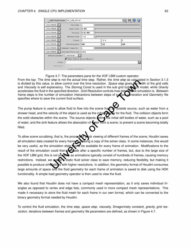
Univers

ity of

Cap

e Tow

n


Figure 4.7: The parameters pane for the VOF LBM custom operator.From the top: The time step is not the actual time step. Rather, the time step as calculated in Section 3.1.3is divided by this value, to allow control over the time resolution. Space step gives the width of the grid cellsand Viscosity is self explanatory. The Stomog Const is used in the sub grid turbulence model, while Gravityaccelerates the fluid in the specified direction. Grid Resolution controls how detailed the simulation is. Betweenframe steps is the number of simulation interactions between steps of surface generation and Geometry filespecifies where to save the current fluid surface.

The pump feature is used to allow fluid to flow into the scene from an outside source, such as water from ashower head, and the velocity of the object is used as the initial velocity for the fluid. The collision objects formthe solid obstacles within the scene. The source objects define the initial still bodies of water, such as a poolof water, and the sink feature allows the absorption of water from a scene, to prevent a scene becoming totallyfilled.

To allow scene scrubbing, that is, the process of quick viewing of different frames of the scene, Houdini savesall simulation data created for every frame by making a copy of the solver class. In some instances, this wouldbe very useful, as the simulation state would be available for every frame of animation. Modifications to theresult of the simulation could then be made after a specific number of frames, but, due to the large size ofthe VOF LBM grid, this is not possible as animations typically consist of hundreds of frames, causing memoryrestrictions. Instead, we create a static fluid solver class to save memory, reducing flexibility, but making itpossible to produce simulations with higher resolutions. In addition, the geometry format of Houdini consumeslarge amounts of space and the fluid geometry for each frame of animation is saved to disk using the HDKfunctionality. A simple load geometry operator is then used to view the fluid.

We also found that Houdini does not have a compact mesh representation, as it only saves individual tri-angles as opposed to vertex and edge lists, commonly used in more compact mesh representations. Thismade it necessary to store the fluid mesh for each frame in our own format, which can be converted to thebinary geometry format needed by Houdini.

To control the fluid simulation, the time step, space step, viscosity, Smagorinsky constant, gravity, grid res-olution, iterations between frames and geometry file parameters are defined, as shown in Figure 4.7.

Univers

ity of

Cap

e Tow

n


4.4.3 Scene Initialisation

To run a simulation the parameters and features provided via the Houdini user interface must be translatedinto VOF LBM grid information. First, the domain constraint is read from the constraint rectangle. From thisand the grid resolution, we calculate the step values used to find the absolute position of each grid locationin the scene. Each grid location, at index (x, y, z) in the grid, is then compared against the feature objectsto initialise the cell to the appropriate state by assigning obstacle objects, pump objects, sink objects and thesource objects (in that order). A precedence of cell states is defined with obstacle cells taking the highest. Thelowest priority is given to source cells. After the cell states are initialised, the appropriate physical quantitiesfor each of the states need to be initialised in order to run the simulation.

The first important physical effect, not mentioned in the graphics literature, but common knowledge in physics,is that fluid pressure varies linearly with depth when the fluid is placed in a container. A drop of water in midair will not have such a relation, as there is virtually no resistance from air. The pressure, P , at a depth h in thecontainer is given by

P = ρgh. (4.9)

For each fluid cell, we check to see if there are no empty cells between it and an obstacle cell below, signalingthat the fluid cell has a floor below and is held within a container. This assumes that there will always be sidesto the container. If this were not the case, the relation would no longer be linear, but there would still be apressure gradient. The pressure for a fluid cell with a floor is then set to the pressure of the fluid cell aboveit, plus the increment given by equation 4.9 adjusted to the lattice normalised values. If no fluid cell is presentabove a fluid cell or for fluid cells with no floor, the pressure is set to 1.

The pressure values of pump cells are set to slightly above 1, as they will distribute fluid into a scene andthe higher pressure values force out more fluid. This parameter can be changed to achieve different simulationeffects. Lastly, the pressure of the sink cells is set to 1.

The velocity of all cells is initialised to the velocity of the feature supplied to the VOF LBM operator, whichin most cases is zero unless the feature is a pump, in which case the velocity is often specified. Once we knowthe velocity and pressure of each cell, we can use the equilibrium function to set the distribution functions tothe appropriate values.

The mass of all cells is set to 1, unless they are interface cells, in which case a value of 0.4 is used, orsink cells, which have 0 mass. This value is chosen arbitrarily and any value may be chosen. During thesimulation, the mass of sink cells is left constant at zero to absorb as much fluid as possible during massexchange.

4.5 Animation Results

Having created a single CPU implementation that is integrated into the Houdini software package, we now pro-vide an analysis of the effects that can be achieved using this software. The influence of different parametervalues on the simulation is also explored. The test case considered is a drop falling into a pool. Other testscases are examined in the final parallel implementation results in Chapter 6. However, this single test case is

Univers

ity of

Cap

e Tow

n


sufficient to analyse the simulation effects.

In the following subsections, we consider the effect of varying the spatial resolution (∆x), the Smagorinskyconstant (S), the time step (∆t), grid resolution (G) and viscosity (v). Grid artifacts are also considered and,lastly, some performance analysis. Note the spatial resolution is the distance between two cells (on one axisfrom center to center), and is different from the grid resolution, which is a measure of simulation scale.

Unless otherwise stated viscosity is set to 1× 10−5 (the viscosity of water) and gravity to 9.8ms−1.

4.5.1 Spatial Resolution

For the falling drop, the spatial resolution is varied, while the other parameter values are held constant, asgiven in Figure 4.8. The entire animation is 72 frames in length and frame 20 is shown in the figure for differentvalues of ∆x.

The simulation is unstable and very bumpy surfaces are produced until the space resolution reaches 0.0006m.After this point, turbulent effects are captured well, but ultimately the effects are smoothed out at very lowscales. For subsequent tests a spatial resolution of 0.0004m is used as this gives sufficient turbulent be-haviour, while avoiding surfaces that are too bumpy. The VOF method also produces bumpy artifacts, as thesurface is moved within a grid and, thus, low grid resolutions will cause additional surface perturbations.

The reasons for this stability behaviour can be seen in the calculation of 1τ , the relaxation parameter. Now,

τ = 3v ∆t(∆x)2 + 1

2 , with v being the viscosity (see section 3.2.3). Therefore, as ∆x gets larger so τ approaches12 , the region of instability for the LBM [Succi, 2001].

The VOF LBM method presented in this thesis has been shown to have to have a small region of stabilitywith respect to spacial resolution for the viscosity of water. Thus, water needs to be simulated at a scale of1mm-6mm. For different viscosities, the exact values are determined by the stability conditions. Most of thesimulations for film applications require large amounts of fluid, so larger grid sizes will be required for suchapplications. Sometimes large scales may be required, however, for such applications, as long the effect looksgood, it is usable. Water behaviour has many similarities at different scales, and one scale can be used toapproximate another.

4.5.2 Smagorinsky constant

Four out of five parameters are kept constant, the values used are provided Figure 4.9, while the value ofthe Smagorinsky constant is varied. In the figure, frame 27 of the animation was used, as it illustrates thedifferences due to the constant more effectively than frame 20.

Higher values for this constant smooth out the fluid behaviour, as the viscosity is artificially increased in regionsof high fluid stress, allowing the LBM to remain stable. Again, the appropriate value is not fixed and artists cancreate different effects by modifying this parameter. For further analysis, the constant value is set at 0.03, asrecommended by Thurey [2007].

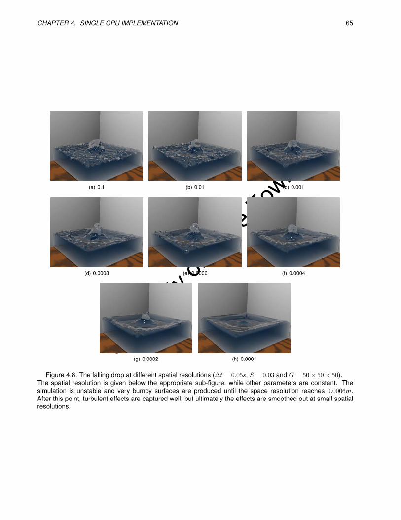
Univers

ity of

Cap

e Tow

n


(a) 0.1 (b) 0.01 (c) 0.001

(d) 0.0008 (e) 0.0006 (f) 0.0004

(g) 0.0002 (h) 0.0001

Figure 4.8: The falling drop at different spatial resolutions (∆t = 0.05s, S = 0.03 and G = 50× 50× 50).The spatial resolution is given below the appropriate sub-figure, while other parameters are constant. Thesimulation is unstable and very bumpy surfaces are produced until the space resolution reaches 0.0006m.After this point, turbulent effects are captured well, but ultimately the effects are smoothed out at small spatialresolutions.

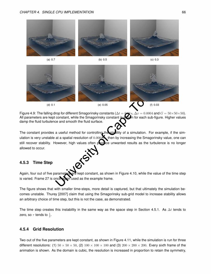
Univers

ity of

Cap

e Tow

n


(a) 0.7 (b) 0.5 (c) 0.3

(d) 0.1 (e) 0.05 (f) 0.03

Figure 4.9: The falling drop for different Smagorinsky constants (∆t = 0.01s, ∆x = 0.0004 andG = 50×50×50).All parameters are kept constant, while the Smagorinsky constant is shown for each sub-figure. Higher valuesdamp the fluid turbulence and smooth the fluid surface.

The constant provides a useful method for controlling the stability of a simulation. For example, if the sim-ulation is very unstable at a spatial resolution of 0.0001m, then by increasing the Smagorinsky value, one canstill recover stability. However, high values often produce unwanted results as the turbulence is no longerallowed to occur.

4.5.3 Time Step

Again, four out of five parameters are kept constant, as shown in Figure 4.10, while the value of the time stepis varied. Frame 27 is once again used as the example frame.

The figure shows that with smaller time-steps, more detail is captured, but that ultimately the simulation be-comes unstable. Thurey [2007] claim that using the Smagorinsky sub-grid model to increase stability allowsan arbitrary choice of time step, but this is not the case, as demonstrated.

The time step creates this instability in the same way as the space step in Section 4.5.1. As ∆t tends tozero, so τ tends to 1

2 .

4.5.4 Grid Resolution

Two out of the five parameters are kept constant, as shown in Figure 4.11, while the simulation is run for threedifferent resolutions: (1) 50 × 50 × 50, (2) 100 × 100 × 100 and (3) 200 × 200 × 200. Every sixth frame of theanimation is shown. As the domain is cubic, the resolution is increased in proportion to retain the symmetry,

Univers

ity of

Cap

e Tow

n


(a) 0.033 (b) 0.025 (c) 0.02

(d) 0.0166 (e) 0.0143 (f) 0.0125

(g) 0.01111 (h) 0.01

Figure 4.10: The falling drop for different time steps (∆x = 0.0004m, S = 0.03 and G = 50× 50× 50).Four out of five parameters are kept constant, while the time step is shown for each sub-figure. A smaller timestep per LBM iteration allows more detail to be simulated, but the fluid becomes more energetic and finally forvery small time steps, it becomes unstable.

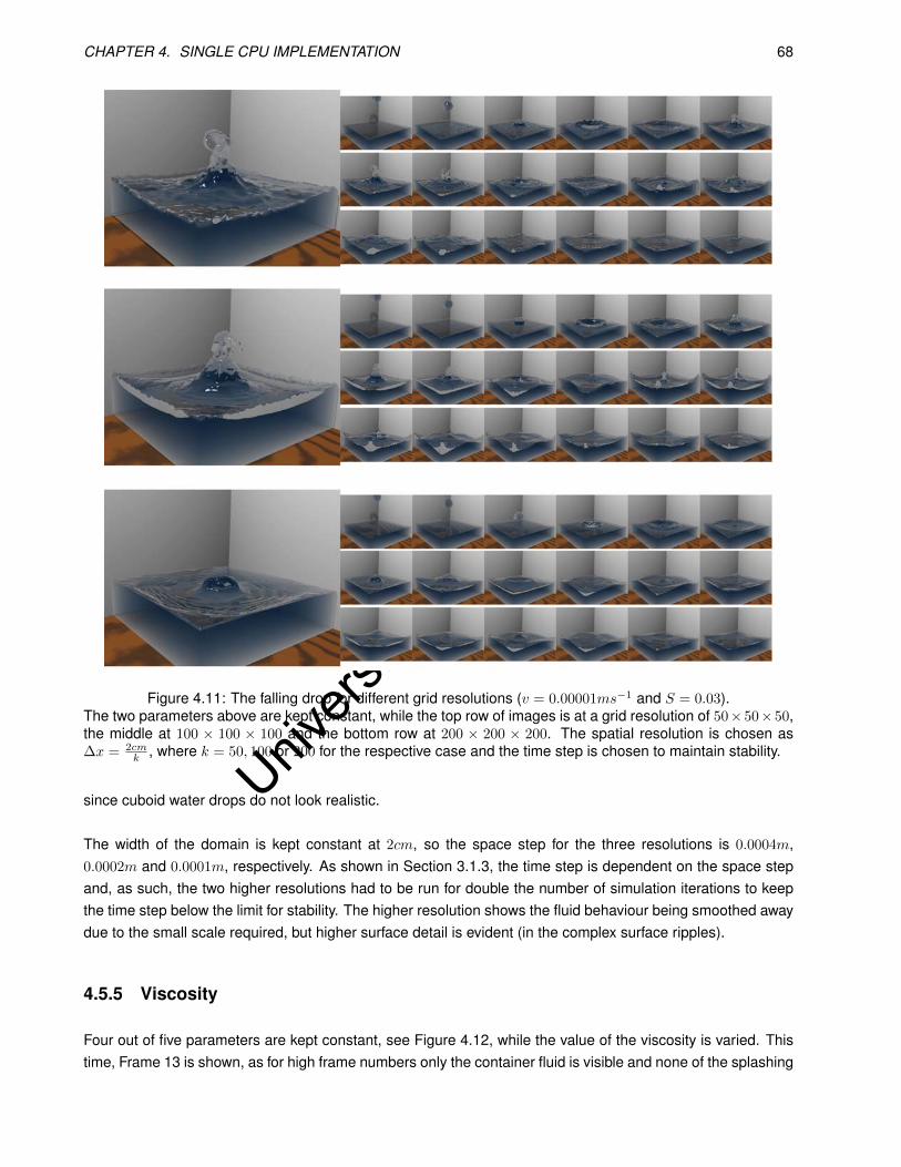
Univers

ity of

Cap

e Tow

n


Figure 4.11: The falling drop for different grid resolutions (v = 0.00001ms−1 and S = 0.03).The two parameters above are kept constant, while the top row of images is at a grid resolution of 50×50×50,the middle at 100 × 100 × 100 and the bottom row at 200 × 200 × 200. The spatial resolution is chosen as∆x = 2cm

k , where k = 50, 100 or 200 for the respective case and the time step is chosen to maintain stability.

since cuboid water drops do not look realistic.

The width of the domain is kept constant at 2cm, so the space step for the three resolutions is 0.0004m,0.0002m and 0.0001m, respectively. As shown in Section 3.1.3, the time step is dependent on the space stepand, as such, the two higher resolutions had to be run for double the number of simulation iterations to keepthe time step below the limit for stability. The higher resolution shows the fluid behaviour being smoothed awaydue to the small scale required, but higher surface detail is evident (in the complex surface ripples).

4.5.5 Viscosity

Four out of five parameters are kept constant, see Figure 4.12, while the value of the viscosity is varied. Thistime, Frame 13 is shown, as for high frame numbers only the container fluid is visible and none of the splashing

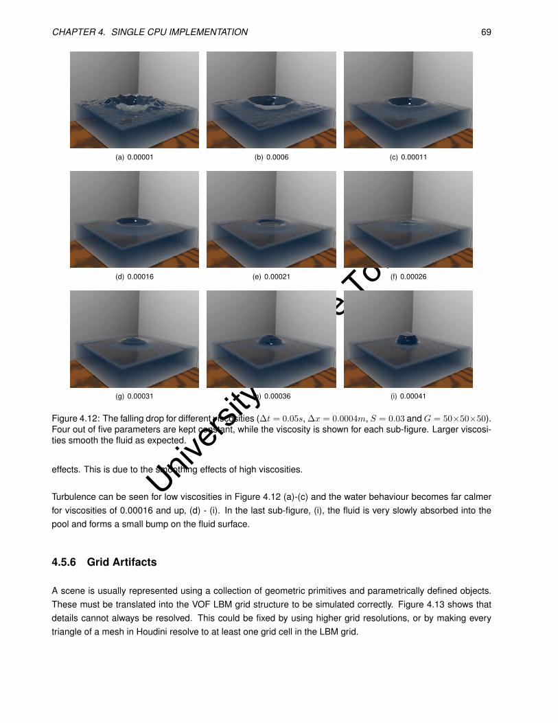
Univers

ity of

Cap

e Tow

n


(a) 0.00001 (b) 0.0006 (c) 0.00011

(d) 0.00016 (e) 0.00021 (f) 0.00026

(g) 0.00031 (h) 0.00036 (i) 0.00041

Figure 4.12: The falling drop for different viscosities (∆t = 0.05s, ∆x = 0.0004m, S = 0.03 andG = 50×50×50).Four out of five parameters are kept constant, while the viscosity is shown for each sub-figure. Larger viscosi-ties smooth the fluid as expected.

effects. This is due to the smoothing effects of high viscosities.

Turbulence can be seen for low viscosities in Figure 4.12 (a)-(c) and the water behaviour becomes far calmerfor viscosities of 0.00016 and up, (d) - (i). In the last sub-figure, (i), the fluid is very slowly absorbed into thepool and forms a small bump on the fluid surface.

4.5.6 Grid Artifacts

A scene is usually represented using a collection of geometric primitives and parametrically defined objects.These must be translated into the VOF LBM grid structure to be simulated correctly. Figure 4.13 shows thatdetails cannot always be resolved. This could be fixed by using higher grid resolutions, or by making everytriangle of a mesh in Houdini resolve to at least one grid cell in the LBM grid.

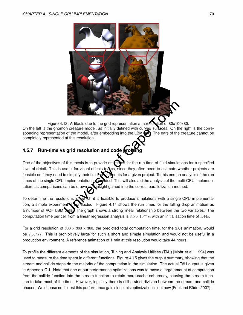
Univers

ity of

Cap

e Tow

n


Figure 4.13: Artifacts due to the grid representation at a resolution of 80x100x80.On the left is the gnomon creature model, as initially defined with curved surfaces. On the right is the corre-sponding representation of the model, after embedding into the LBM grid. The ears of the creature cannot becompletely represented at this resolution.

4.5.7 Run-time vs grid resolution and code profiling

One of the objectives of this thesis is to provide estimates for the run time of fluid simulations for a specifiedlevel of detail. This is useful for visual effects teams, since they often need to estimate whether projects arefeasible or if they need to simplify their fluid requirements for a given project. To this end an analysis of the runtimes of the single CPU implementation is provided. This will also aid the analysis of the multi-CPU implemen-tation, as comparisons can be drawn and insight gained into the correct parallelization method.

To determine the resolutions for which it is feasible to produce simulations with a single CPU implementa-tion, a simple experiment is conducted. Figure 4.14 shows the run times for the falling drop animation asa number of VOF LBM cells. The graph shows a strong linear relationship between the two variables. Thecomputation time per cell from a linear regression analysis is 3.5× 10−4s, with an initialisation time of 1.44s.

For a grid resolution of 300 × 300 × 300, the predicted total computation time, for the 3.6s animation, wouldbe 2.65hrs. This is prohibitively large for such a short and simple simulation and would not be useful in aproduction environment. A reference animation of 1 min at this resolution would take 44 hours.

To profile the different elements of the simulation, Tuning and Analysis Utilities (TAU) [Mohr et al., 1994] wasused to measure the time spent in different functions. Figure 4.15 gives the output summary, showing that thestream and collide steps do the majority of the computation in the simulation. The actual TAU output is givenin Appendix C.1. Note that one of our performance optimizations was to move a large amount of computationfrom the collide function into the stream function to retain more cache coherency, causing the stream func-tion to take most of the time. However, logically there is still a strict division between the stream and collidephases. We choose not to test this performance gain since this optimization is not new [Pohl and Rüde, 2007].

Univers

ity of

Cap

e Tow

n


y = 3.54E-04x + 1.44E+00

0

50

100

150

200

250

300

350

400

0 100 200 300 400 500 600 700 800 900 1,000 1,100

Sim

ula

tio

n R

un

tim

e (

s)

Number of LBM scene cells

Thousands

Single CPU Runtime for 3.6s drop animation

Figure 4.14: The time taken to produce the 3.6s falling drop animation for different resolutions.

Figure 4.15: Percentage of time spent in each of the steps during a simulation.

Quantity Type Size(bytes) PercentageMass float 4 2.1

Pressure float 4 2.1Fluid Fraction float 4 2.1

Velocity float[3] 12 6.6Distribution functions 2× float[19] 152 83.1

Neighbour Counts char[3] 3 1.6Queue Position int 4 2.1

TOTAL 183 100

Table 4.2: The space taken up by one cell in the VOF LBM implementation.

Univers

ity of

Cap

e Tow

n


Source

Domain

(a) Still pond

Figure 4.16: Still pond test case.

Figure 4.17: A analysis of the operations per cell in the stream and collide steps for the pond test case.The operation counts section indicates the total number of operations for the given step, while the percentagespreads gives the percentage of operations from the sub-step shown. The breakdown subsections give thespreads of the operations within the subsection. This analysis is for the still pond test case, as the cell distri-bution is predictable, but is a good indication of where the LBM computation is performed. It is interesting tonote the collide step forms the majority of computation and the Smagorinsky stability forms a large percentageof these operations.

Univers

ity of

Cap

e Tow

n


0

500

1000

1500

2000

2500

3000

3500

4000

4500

5000

0 50 100 150 200 250 300 350

Me

mo

ry (

Mb

)

Grid Resolution of k X k X k, where k is indicated on the axis

Memory Usage of VOF LBM

Figure 4.18: Memory usage of the VOF LBM implementation.The graph shows that the memory usage becomes prohibitively large above a grid resolution of 200×200×200cells.

Figure 4.17 shows a summary of the distribution of memory accesses, floating point and integer operationswithin the stream and collide functions for the test case illustrated in Figure 4.16. This test case is used as thefluid remains constant and is more easily analysed. The LBM has strong reliance on memory accesses andfloating point operations. Notice that the interface cells have more memory accesses due to the VOF masstracking. Most of the simulation time is spent in the stream and collide steps, with the majority of operationsin the collide step. This is especially true for the fluid cells, which will normally form the majority of the fluid inthe scene unless the fluid in the scene consists of a large number of thin sheets. The Smagorinsky stabilityforms a large percentage of these operations (on average above 50% of the total cell operations for fluid cellsand just under 50% for interface cells with respect to the stream and collide steps). The complexity of the VOFLBM is thus increased dramatically to main stability. A cheaper stabilization model would be a good area offurther research to improve the computation efficiency of the VOF LBM algorithm.

Indeed, memory is a significant consideration of the LBM, as a large amount of storage space is neededper cell. Table 4.2 shows that 183 bytes of space are required per cell. Figure 4.18 shows the scaling of thememory usage with respect to the grid resolution and the memory used becomes very large above a resolutionof 200× 200× 200. To simulate large amounts of fluid, more then 4GB of memory is typically necessary.

Both the large amounts of memory required and the large run times for a simulation make the VOF LBMalgorithm unattractive for use on a single PC. As most of the work done in the algorithm is in the stream andcollide steps, both of which are per cell local operations, the algorithm would benefit considerably from paral-lelization. However, the large amount of data needed in the LBM might cause problems if the communication

Univers

ity of

Cap

e Tow

n


between process or threads is slow.

4.6 Conclusion

The results have shown that the VOF LBM is a viable option for creating fluid simulations. However, it has notproven as robust as we hoped. Water behaviour is adequately captured by the method and by using smallertime steps, more turbulence can be captured (as shown in section 4.5.3). However, this cannot be an arbitrarychoice as the simulation becomes unstable for very small time steps. The stability conditions for a given vis-cosity do not allow for much parameter tweaking, unless physically realistic results are required.

At lower grid resolutions the fluid surface is, in general, more bumpy, and the higher resolution smooths thebumps and gives more detail. Higher resolutions are also favourable for obstacle interaction, as more detailcan then be resolved. However, they come at memory and computation costs (as shown in Section 4.5.4). TheLBM needs significant amounts of memory for such resolutions and will benefit from a large cache. Appropriatecache optimisations are also advisable.

From the performance analysis in Section 4.5.7, it becomes clear that it is only attractive to simulate sceneswith low resolutions on a single desktop. If larger scenes are required then using a cluster environment will beadvantageous, as this will provide extra processing power and memory. In addition, to properly analyse thesimulations possible with the VOF LBM, larger more complex scenes will be required. We perform this analysisin Chapter 6.

Univers

ity of

Cap

e Tow

n

Chapter 5

Parallelization

5.1 Introduction

This chapter describes the conversion of our single CPU fluid simulation (detailed in Chapters 3 and 4) into amulti-CPU version. The intention is to reduce the computation time required to generate the simulations. Ourtarget platform is be any form of computational cluster: a group of computers that are connected by a highspeed network.

The single CPU simulation runs on the same computer as the interface (Houdini) and is tightly bound toHoudini as a plug-in. The multi-CPU version uses the same interface, but the simulation computation is farmedoff to a back-end cluster by the plug-in, which generates and returns the fluid surface to Houdini. In simpleterms, the back-end system uses multiple versions of the single CPU version running on each available CPU,with added logic for communication.

Load balancing is a problem for many physical simulations [Wilkinson and Allen, 1998]. The multi-CPU simu-lation should divide the workload up evenly among each of the processors to achieve an optimal load balance.For example, if we have 10 units of work and 10 CPUs, each of the CPUs could be given one unit of work.Our problem, however, is not so clearly defined, as the work to be performed is a complete simulation. This isa repetitive process of updating each grid location in the domain for each time step. As explained in Section3, this requires information from neighbouring cells and, hence, the assignment of grid locations to a pool ofCPU’s must be efficient. Finally, each CPU should have all the required information to update the assignedgrid locations.

The problem is further complicated by the fact that each grid location does not require the same amountof time to update. Trivially, a fluid cell takes far longer to update than an empty cell, although the difference intime required between a fluid cell and interface cell is far less (see Section 4.5.7 for a comparison). Even if wecould perfectly estimate the difference in update time, fluid simulation is dynamic in nature and we cannot besure of the scene fluid division ahead of time. Hence, we make use of load balancing to improve the algorithmefficiency.

The first step is the design of the back-end system, which makes use of the popular Message Passing In-

75

Univers

ity of

Cap

e Tow

n

CHAPTER 5. PARALLELIZATION 76

terface (MPI) protocol [Gropp et al., 1999]. This runs the simulation and returns the results to Houdini. InSection 2.6 we discuss previous approaches and parallel concepts to gain insight into the design. Using theseideas and definitions, the design of the parallel LBM implementation for this thesis is presented in Section 5.2,while the specific implementation details are given in Section 5.3.

5.2 Design

5.2.1 Algorithm Classification

The LBM algorithm can be converted to a parallel algorithm in a coarse grained fashion by splitting up thestream and collide loops. Every cell can be updated independently from the previous time-step’s data forthe neighbouring cell. Hence, we expect Ts Tp, and that the algorithm should parallelize well. There is amedium level of data dependency, since it is a cellular automata system and requires neighbouring cell infor-mation to update a grid cell. This means synchronisation will be needed for every iteration of the simulation,which impacts on performance. Indeed, as previously mentioned, the problem is one of deciding which CPUwill process which grid cell. The only sequential operations are the division of a given scene into units thatcan be processed by each CPU and the collection of the resulting fluid mesh once a frame of simulation iscomplete. There are additional operations that have to be run by every slave process, namely new operations(communication not included), that each CPU will have to perform to synchronize with neighbouring nodes.This extra time is created by the need to post- and pre- process messages.

We now discuss possible decompositions of the problem.

5.2.2 Master/Slave Division and Problem Decomposition

We use the master/slave model for parallelization, with 1 master and N slaves. However, there are many pos-sible master/slave configurations. The master will always assign work units to the slaves and collate results.

One possible model has the master transmit the data for a number of grid cells to a slave, the slave thenupdates those grid cells and returns the data. This approach allows each slave to request work when it is idle.It does not require slave synchronization (as each slave will receive a complete set of data required to updatethe cells) and will have inherent load balancing properties. With this model, the total update time for k grid cellsfor one iteration can be modelled as

2Tstartup + 2k × cell data sizeTdata + Tcell update × k,

where Tstartup and Tdata are as defined in Section 2.6.2. The transmission of the fluid geometry is not takeninto account. Tcell update is expected to be small and the time required to transmit the required cell data willmost likely dominate the update time for k cells. Additionally, the synchronization of each slave with the mastercauses a potential bottleneck for the simulation. The master also needs enough memory to store the entirescene. An entire scene, which can easily take up 2GB or more memory, will be transmitted every iteration.

Alternatively, the scene can be distributively stored across the compute nodes. The master then assigns

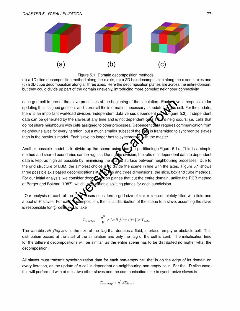
Univers

ity of

Cap

e Tow

n


Figure 5.1: Domain decomposition methods.(a) a 1D slice decomposition method along the x-axis, (c) a 2D box decomposition along the x and z axes and(c) a 3D cube decomposition along all three axes. Here the decomposition planes are across the entire domain,but they could divide up part of the domain unevenly, introducing more complex neighbour connectivity.

each grid cell to one of the slave processes at the beginning of the simulation. Each slave is responsible forupdating the assigned grid cells and stores all the information necessary to update the grid cell. For the update,there is an important workload division: independent data versus dependent data (Figure 5.3). Independentdata can be generated by the slaves at any time and is not dependent on a slave’s neighbours, i.e. cells thatdo not share neighbours with cells assigned to other processes. Dependent data requires communication fromneighbour slaves for every iteration, but a much smaller subset of the data is transmitted to synchronize slavesthan in the previous model. Each slave no longer has to synchronize with the master.

Another possible model is to divide up the scene using domain partitioning (Figure 5.1). This is a simplemethod and shared boundaries can be regular. During the division, the ratio of independent data to dependentdata is kept as high as possible by minimising the shared surface between neighbouring processes. Due tothe grid structure of LBM, the simplest choice is to divide the scene in line with the axes. Figure 5.1 showsthree possible axis based decompositions in one, two and three dimensions: the slice, box and cube methods.For our initial analysis, we consider decomposition planes that cut the entire domain, unlike the RCB methodof Berger and Bokhari [1987], which uses variable splitting planes for each subdivision.

Our analysis of each of the three cases considers a grid size of n × n × n completely filled with fluid anda pool of P slaves. For each decomposition, the initial distribution of the scene to a slave, assuming the slaveis responsible for n

3

P cells, would take

Tstartup +n3

P× cell f lag size × Tdata.

The variable cell f lag size is the size of the flag that denotes a fluid, interface, empty or obstacle cell. Thisdistribution occurs at the start of the simulation and only the flag of the cell is sent. The initialisation timefor the different decompositions will be similar, as the entire scene has to be distributed no matter what thedecomposition.

All slaves must transmit synchronization data for each non-empty cell that is on the edge of its domain onevery iteration, as the update of a cell is dependent on neighbouring non-empty cells. For the 1D slice case,this will performed with at most two other slaves and the communication time to synchronize slaves is

Tstartup + n2xTdata,

Univers

ity of

Cap

e Tow

n


for each iteration, where x is the size of data that needs to be sent for correct synchronisation of a cell. Theexact amount of data that needs to be synchronised will be defined in later sections. For the different decom-positions, x remains constant and the value is not considered here. We assume here that data can be sentto more than one slave simultaneously (see section 5.3.3 for details on non-blocking communication). For thisreason, we also neglect the synchronisation on the corners, as the bulk of the synchronisation will happen onflat surfaces.

For a 2D box division of u by v, where u × v = P , with these being optimal integer values to maximizethe number of independent cells, we get

Tstartup + n2xTdata ×1

v.

For numbers which are not the product of two integers greater than one, the next closests nicely factorizablenumber can be chosen. For example if we wanted seven slaves, u and v would not be obvious and we thencan have eight slaves instead. Further, without loss of generality, we assume u > v. In this case, each slavewill need to synchronize with, at most, 8 other slaves, but 4 of the slaves will require far less communication,as they are only neighbours on a corner edge.

For 3D cubes, each slave will have to synchronize with, at most 18 others and the communication time will be

Tstartup + n2xTdata ×1

vw,

where the division is u by v by w and u× v × w = P with u > v > w.

From this, we can see that of the three methods, the communication time for the 3D decomposition scalesbest, followed by the 2D and lastly the 1D case. However, this does not necessarily mean that these are thebetter options as they introduce added complexities and more operations are performed per iteration to man-age the simulation. As mentioned previously, the workload of the simulation will not be evenly distributed andin the next section we will look at what effects this will have on our design.

5.2.3 Load Balancing

Thus far we have described a system where the simulation data is passed once from the master to a numberof slaves that then update the simulation and send the resultant fluid surface back to the master. For eachiteration, the slaves must synchronize with each other. This means that one iteration is only as fast as theslowest slave, as all the slaves must wait for that slave to complete its computation. Through load balancing,we aim to make each slave run for the same time per iteration and, therefore, maximise efficiency.

Körner et al. [2006] suggest, but do not implement, a 1D load balancing scheme for the LBM. The schemeshifts the domain decomposition when a imbalance is detected. This is detected by measuring the wait time forsynchronisations with neighbouring processes. When the wait time is overly large, a load balance is initiatedand a plane (as it is a slice decomposition) of cells is fetched from the neighbour that causes the wait. Thismethod works with all three of the domain decompositions and, thus, the load balance communication willscale the similarly to the synchronization communication. Although all cell data is transmitted during a loadbalancing phase, we can optimize the synchronization by only sending a subset of cell data.

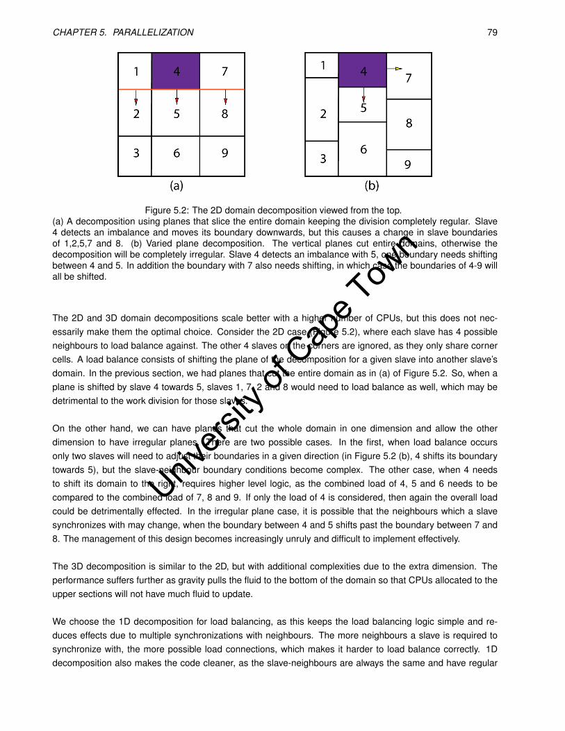
Univers

ity of

Cap

e Tow

n


Figure 5.2: The 2D domain decomposition viewed from the top.(a) A decomposition using planes that slice the entire domain keeping the division completely regular. Slave4 detects an imbalance and moves its boundary downwards, but this causes a change in slave boundariesof 1,2,5,7 and 8. (b) Varied plane decomposition. The vertical planes cut entire domains, otherwise thedecomposition will be completely irregular. Slave 4 detects an imbalance with 5, one boundary needs shiftingbetween 4 and 5. In addition the boundary with 7 also needs shifting, in which case the boundaries of 4-9 willall be shifted.

The 2D and 3D domain decompositions scale better with a higher number of CPUs, but this does not nec-essarily make them the optimal choice. Consider the 2D case (Figure 5.2), where each slave has 4 possibleneighbours to load balance against. The other 4 slaves on the corners are ignored, as they only share cornercells. A load balance consists of shifting the plane of the decomposition for a given slave into another slave’sdomain. In the previous section, we had planes that cut the entire domain as in (a) of Figure 5.2. So, when aplane is shifted by slave 4 towards 5, slaves 1, 7, 2 and 8 would need to load balance as well, which may bedetrimental to the work division for those slaves.

On the other hand, we can have planes that cut the whole domain in one dimension and allow the otherdimension to have irregular planes. There are two possible cases. In the first, when load balance occursonly two slaves will need to adjust their boundaries in a given direction (in Figure 5.2 (b), 4 shifts its boundarytowards 5), but the slave-neighbour boundary conditions become complex. The other case, when 4 needsto shift its domain to the right, requires higher level logic, as the combined load of 4, 5 and 6 needs to becompared to the combined load of 7, 8 and 9. If only the load of 4 is considered, then again the overall loadcould be detrimentally effected. In the irregular plane case, it is possible that the neighbours which a slavesynchronizes with may change, when the boundary between 4 and 5 shifts past the boundary between 7 and8. The management of this design becomes increasingly unruly and difficult to implement effectively.

The 3D decomposition is similar to the 2D, but with additional complexities due to the extra dimension. Theperformance suffers further as gravity pulls the fluid to the bottom of the domain so that CPUs allocated to theupper sections will not have much fluid to update.

We choose the 1D decomposition for load balancing, as this keeps the load balancing logic simple and re-duces effects due to multiple synchronizations with neighbours. The more neighbours a slave is required tosynchronize with, the more possible load connections, which makes it harder to load balance correctly. 1Ddecomposition also makes the code cleaner, as the slave-neighbours are always the same and have regular

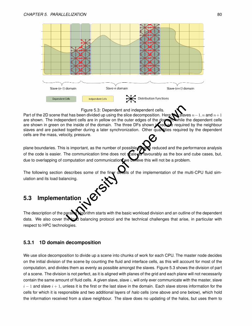
Univers

ity of

Cap

e Tow

n


Figure 5.3: Dependent and independent cells.Part of the 2D scene that has been divided up using the slice decomposition. Here, the slaves n−1, n and n+1are shown. The independent cells are in yellow on the outer edges of the domain, while the dependent cellsare shown in green on the inside of the domain. The three DFs shown in red are required by the neighbourslaves and are packed together during a later synchronization. Other quantities required by the dependentcells are the mass, velocity, pressure.

plane boundaries. This is important, as the number of possible bugs is reduced and the performance analysisof the code is easier. The communication time does not scale as favourably as the box and cube cases, but,due to overlapping of computation and communication, we believe this will not be a problem.

The following section describes some of the finer details of the implementation of the multi-CPU fluid sim-ulation and its load balancing.

5.3 Implementation

The description of the parallel algorithm starts with the basic workload division and an outline of the dependentdata. We also cover the load balancing protocol and the technical challenges that arise, in particular withrespect to HPC technologies.

5.3.1 1D domain decomposition

We use slice decomposition to divide up a scene into chunks of work for each CPU. The master node decideson the initial division of the scene by counting the fluid and interface cells, as this will account for most of thecomputation, and divides them as evenly as possible amongst the slaves. Figure 5.3 shows the division of partof a scene. The division is not perfect, as it is aligned with planes of the grid and each plane will not necessarilycontain the same amount of fluid cells. A given slave, slave i, will only ever communicate with the master, slavei− 1 and slave i+ 1, unless it is the first or the last slave in the domain. Each slave stores information for thecells for which it is responsible and two additional layers of halo cells (one above and one below), which holdthe information received from a slave neighbour. The slave does no updating of the halos, but uses them to

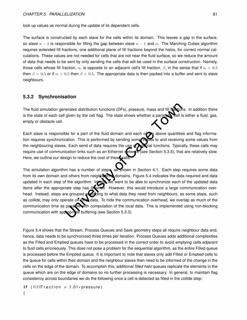
Univers

ity of

Cap

e Tow

n


look up values as normal during the update of its dependent cells.

The surface is constructed by each slave for the cells within its domain. This leaves a gap in the surface,so slave n − 1 is responsible for filling the gap between slave n − 1 and n. The Marching Cubes algorithmrequires extended fill fractions, one additional plane of fill fractions beyond the halos, for correct normal cal-culations. These values are not needed for cells that are not near the fluid surface, so we reduce the amountof data that needs to be sent by only sending the cells that will be used in the surface construction. Namely,those cells whose fill fraction, α, is opposite to an adjacent cell’s fill fraction, β, in the sense that if α < 0.5

then β > 0.5 or if α > 0.5 then β < 0.5. The appropriate data is then packed into a buffer and sent to slaveneighbours.

5.3.2 Synchronisation

The fluid simulation generates distribution functions (DFs), pressure, mass and fill fractions. In addition thereis the state of each cell given by the cell flag. The state shows whether a particular cell is either a fluid, gas,empty or obstacle cell.

Each slave is responsible for a part of the fluid domain and each of the above quantities and flag informa-tion requires synchronization. This is performed by sending some values to and receiving some values fromthe neighbouring slaves. Each send of data requires the use of external functions. Typically, these calls mayrequire use of communication links such as an Ethernet network (see Section 5.3.5), that are relatively slow.Here, we outline our design to reduce the cost of these calls.

The simulation algorithm has a number of steps, as shown in Section 4.1. Each step requires some datafrom its own domain and others from neighbouring domains. Figure 5.4 indicates the data required and dataupdated in each step of the algorithm. Ideally, we want to be able to synchronize each of the updated dataitems after the appropriate step has finished. However, this would introduce a large communication over-head. Instead, steps are grouped according to what data they need from neighbours, as some steps, suchas collide, may only operate on local data. To hide the communication overhead, we overlap as much of thecommunication time as possible with computation of the local data. This is implemented using non-blockingcommunication with appropriate buffering (see Section 5.3.3).

Figure 5.4 shows that the Stream, Process Queues and Save geometry steps all require neighbour data and,hence, data needs to be synchronized three times per iteration. Process Queues adds additional complexitiesas the Filled and Emptied queues have to be processed in the correct order to avoid emptying cells adjacentto fluid cells erroneously. This does not pose a problem for the sequential algorithm, as the entire Filled queueis processed before the Emptied queue. It is important to note that slaves only add Filled or Emptied cells tothe queue for cells within their domain and the neighbour slaves then need to be informed of the change in thecells on the edge of the domain. To accomplish this, additional filled halo queues replicate the elements in thequeue which are on the edge of domains so no further processing is necessary. In general, to maintain flagconsistency across boundaries we do the following once a cell is detected as filled in the collide step:

i f ( f i l l F r a c t i o n > 1.01∗ pressure )

Univers

ity of

Cap

e Tow

n


Figure 5.4: Simulation steps and required quantities.This figure shows the individual steps of the sequential simulation and the required data for each step. Eachsteps operates on a cell and either only uses data contained in the current cell (shown in plain text) or fromneighbouring and current cells (shown in red). The filled and emptied queues store which cells are changingfrom an interface cell to a fluid cell and an interface cell to an empty cell.

for ad j i n ad jacent c e l l si f adj i n emptiedQueue

remove from queue

mark ad j as not_al lowed_to_emptyend

i f cu r ren tCe l lX == 0 or cu r ren tCe l lX == width−1 thenadd c u r r e n t C e l l to f i l ledHaloQueue

This ensures that the information stored in filled halo queues will be correct even after the subsequent ProcessQueues step is performed.

The emptied halo queue is formed by a post process of cells in the x = 1 and x = width − 1 plane, tosee which ones are marked as emptied. The two queues can now be sent to their neighbours, as they areconsistent and correctly ordered, and thus usable in updating their domain. The halo queues do not, however,tell the slaves when an interface cell has been added to the halo plane, which causes inconsistencies in thecell neighbour counts. An additional operation is performed to recount these values.

The two points of synchronization, Sync-A and Sync-B, are shown in Figure 5.5, with a small step re-ordering.These are before the stream step and after the collide step, respectively. The fill fraction is changed due to theredistribution of mass from filled or emptied cells in the process queues step. The difference in fill fraction is onthe order of 1% of the fill fraction as the mass that is redistributed is only from cells that are within 1% of fillingor emptying. This value is averaged with neighbouring fill fractions in the stream step, so the influence on the

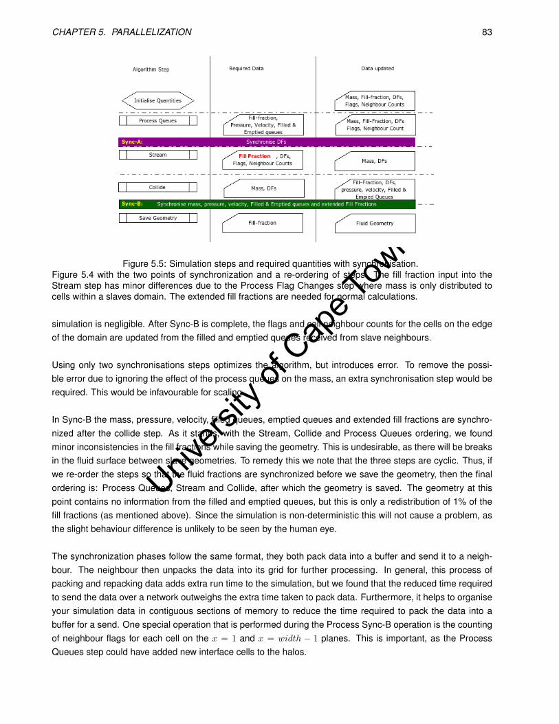
Univers

ity of

Cap

e Tow

n


Figure 5.5: Simulation steps and required quantities with synchronisation.Figure 5.4 with the two points of synchronization and a re-ordering of steps. The fill fraction input into theStream step has minor differences due to the Process Flag Changes step where mass is only distributed tocells within a slaves domain. The extended fill fractions are needed for normal calculations.

simulation is negligible. After Sync-B is complete, the flags and cell neighbour counts for the cells on the edgeof the domain are updated from the filled and emptied queues received from slave neighbours.

Using only two synchronisations steps optimizes the algorithm, but introduces error. To remove the possi-ble error due to ignoring the effect of the process queues on the mass, an extra synchronisation step would berequired. This would be infavourable for scaling.

In Sync-B the mass, pressure, velocity, filled queues, emptied queues and extended fill fractions are synchro-nized after the collide step. As it stands, with the Stream, Collide and Process Queues ordering, we foundminor inconsistencies in the fill fractions while saving the geometry. This is undesirable, as there will be breaksin the fluid surface between slave geometries. To remedy this we note that the three steps are cyclic. Thus, ifwe re-order the steps so that the fluid fractions are synchronized before we save the geometry, then the finalordering is: Process Queues, Stream and Collide, after which the geometry is saved. The geometry at thispoint contains no information from the filled and emptied queues, but this is only a redistribution of 1% of thefill fractions (as mentioned above). Since the simulation is non-deterministic this will not cause a problem, asthe slight behaviour difference is unlikely to be seen by the human eye.

The synchronization phases follow the same format, they both pack data into a buffer and send it to a neigh-bour. The neighbour then unpacks the data into its grid for further processing. In general, this process ofpacking and repacking data adds extra run time to the simulation, but we found that the reduced time requiredto send the data over a network outweighs the extra time taken to pack data. Furthermore, it helps to organiseyour simulation data in contiguous sections of memory to reduce the time required to pack the data into abuffer for a send. One special operation that is performed during the Process Sync-B operation is the countingof neighbour flags for each cell on the x = 1 and x = width − 1 planes. This is important, as the ProcessQueues step could have added new interface cells to the halos.

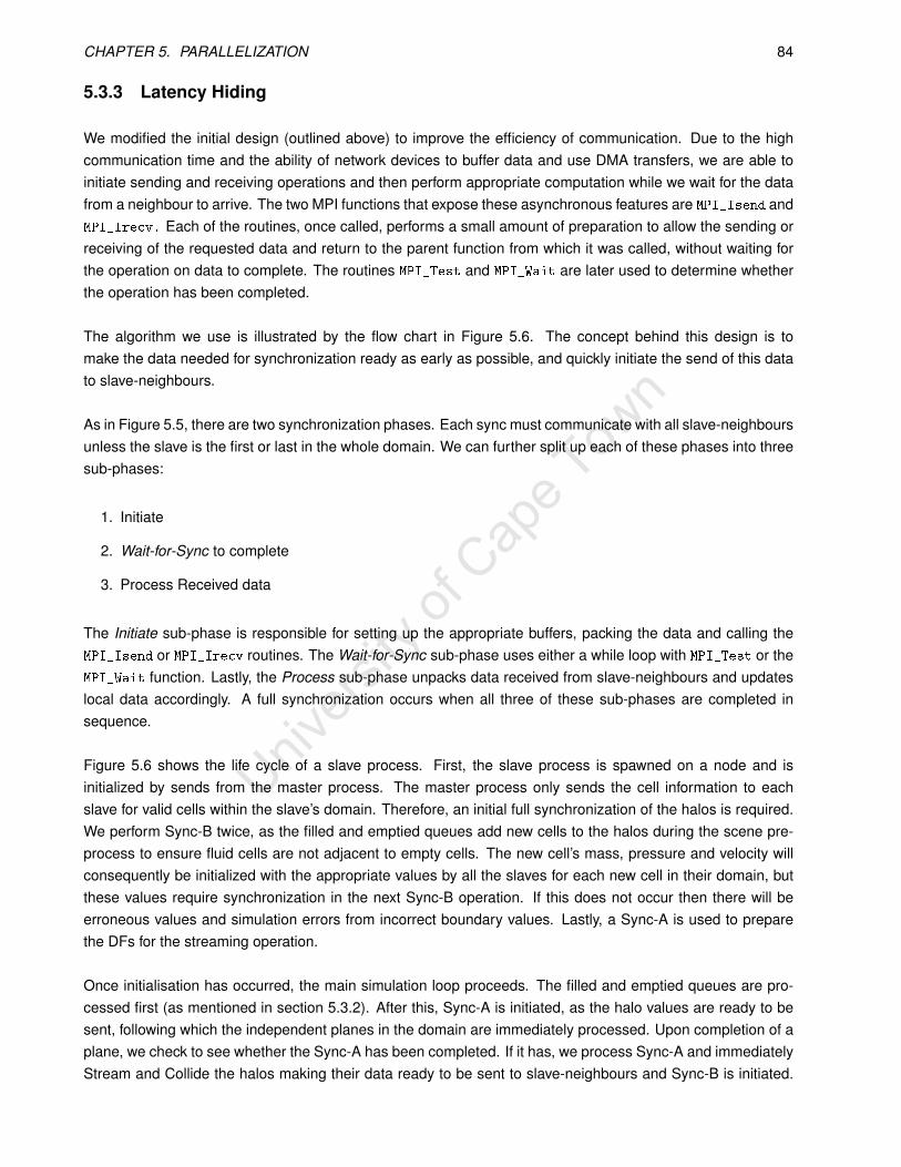
Univers

ity of

Cap

e Tow

n


5.3.3 Latency Hiding

We modified the initial design (outlined above) to improve the efficiency of communication. Due to the highcommunication time and the ability of network devices to buffer data and use DMA transfers, we are able toinitiate sending and receiving operations and then perform appropriate computation while we wait for the datafrom a neighbour to arrive. The two MPI functions that expose these asynchronous features are MPI_Isend andMPI_Irecv. Each of the routines, once called, performs a small amount of preparation to allow the sending orreceiving of the requested data and return to the parent function from which it was called, without waiting forthe operation on data to complete. The routines MPI_Test and MPI_Wait are later used to determine whetherthe operation has been completed.

The algorithm we use is illustrated by the flow chart in Figure 5.6. The concept behind this design is tomake the data needed for synchronization ready as early as possible, and quickly initiate the send of this datato slave-neighbours.

As in Figure 5.5, there are two synchronization phases. Each sync must communicate with all slave-neighboursunless the slave is the first or last in the whole domain. We can further split up each of these phases into threesub-phases:

1. Initiate

2. Wait-for-Sync to complete

3. Process Received data

The Initiate sub-phase is responsible for setting up the appropriate buffers, packing the data and calling theMPI_Isend or MPI_Irecv routines. The Wait-for-Sync sub-phase uses either a while loop with MPI_Test or theMPI_Wait function. Lastly, the Process sub-phase unpacks data received from slave-neighbours and updateslocal data accordingly. A full synchronization occurs when all three of these sub-phases are completed insequence.

Figure 5.6 shows the life cycle of a slave process. First, the slave process is spawned on a node and isinitialized by sends from the master process. The master process only sends the cell information to eachslave for valid cells within the slave’s domain. Therefore, an initial full synchronization of the halos is required.We perform Sync-B twice, as the filled and emptied queues add new cells to the halos during the scene pre-process to ensure fluid cells are not adjacent to empty cells. The new cell’s mass, pressure and velocity willconsequently be initialized with the appropriate values by all the slaves for each new cell in their domain, butthese values require synchronization in the next Sync-B operation. If this does not occur then there will beerroneous values and simulation errors from incorrect boundary values. Lastly, a Sync-A is used to preparethe DFs for the streaming operation.

Once initialisation has occurred, the main simulation loop proceeds. The filled and emptied queues are pro-cessed first (as mentioned in section 5.3.2). After this, Sync-A is initiated, as the halo values are ready to besent, following which the independent planes in the domain are immediately processed. Upon completion of aplane, we check to see whether the Sync-A has been completed. If it has, we process Sync-A and immediatelyStream and Collide the halos making their data ready to be sent to slave-neighbours and Sync-B is initiated.

Univers

ity of

Cap

e Tow

n


Figure 5.6: Flow diagram for each slave process.The operational sub-flows illustrated at the top of the diagram are re-used later. Here, as much computation isoverlapped with communication as possible. Each of the steps are denoted by rectangular boxed, with thesends being colour coded. The full synchronisations are given oval shapes as they perform the initiate, waitand process sub-steps, but do not perform direct computation on cells. Diamonds indicate decisions andcontrol the flow of the program execution.

SUB- FLOW S Load hlal>«l

~.-1.) Par.n.I Pro« ..

Q ...... . 5u1t-1low

II 2.) Re·"'" dom~i n II I 3.) 5endI Re<V pI~ i n I VOf LBM ~II.

II 3.) -=s Queues II < 4.a) f~ 1 Sync:·A > 4.b) f~ 1 Sync:· B

Entry Poi nt

'" Siove initioli"'tioo '"

R=ive i ni ti~ 1 Cell.

FINAUS E

'"

'"

'"

Univers

ity of

Cap

e Tow

n


We then go back and finish the stream and collide operation on the independent data. Finally, after all thenon-halo planes are completed we make sure that the Sync-B has completed and update the halos. Ideally, ifthere is perfect overlapping of computation and communication we will not have to wait at this point. However,this is unlikely and when the wait time is large, it is probable that load balancing is needed.

5.3.4 Load Balancing Protocol

The fluid will not always be evenly distributed across the domain and thus a static partitioning of the domainis not always an efficient strategy for partitioning computation. The dynamic strategy we apply, suggested byKörner et al. [2006], uses movable domain boundaries. We employ a slave-driven, idle process load balancingapproach. Each slave has a set of slave-neighbours with which it synchronizes data. When a slave starts waitstoo long during either Sync-A or Sync-B, load balancing may be required.

The idle time period while waiting for each of the Sync operations to be finished, is stored separately foreach slave-neighbour. If a wait time is larger than a threshold percentage of the total time for the current loadbalancing step, the slave that has been waiting requests a load balance phase from the slave-neighbour inquestion, by sending a message containing the time it has spent waiting. Upon receiving the request, theslave-neighbour will compare the received wait time to its current wait times and if it is appropriately larger, therequest will be acknowledged. In this case, the two slaves go into a load balancing phase, during which thedomains are re-sized. If however, the received wait time is not large enough, the load balancing is denied.

The load balancing phase proceeds as follows (see Figure 5.6):

1. Wait-for-Sync-B and Process Sync-B to ensure local domain consistency,

2. Increase or decrease current domain to cater for adjustment,

3. Send or receive plane of VOF LBM cells due to the change, to or from slave-neighbour,

4. Perform Sync-A and Sync-B operation for halo consistency.

The sending and receiving of any data during the load balance is implemented using blocking communication,as the domains are being restructured. The computation can only resume once the new domains are properlyset-up. It is possible to use non-blocking communication as parts of the domain do remain constant, but thiswould require significant code enhancements, which we believe would outweigh the performance gains.

5.3.5 Technologies

MPI is language independent and has a number of specifications for different languages. We make use of theC and C++ specifications for MPI. There are many implementations of MPI for different platforms, but almostall high performance architectures have at least one. Each implementation has its own merits, some havebeen optimised for specific hardware (e.g., MVAPICH), while others are designed for multiple platforms (e.g.,MPICH). Most of the implementations are very similar, as they follow the specifications closely, and the changefrom one to another, is simply a process of linking in the correct header files and libraries during compilation.

Univers

ity of

Cap

e Tow

n


Cluster Nodes CPUs/Node CPU Type Interconnect Tstart−up Tdata Memory/NodeCRUNCH 9 2 Dual core

2.4GhzXeon

GigabitEthernet

1614µs 119Mbs−1 1GB

CHPC 160 4 Dual core2.4GhzXeon

Infiniband 87.06µs 396Mbs−1 17GB

Table 5.1: The two different clusters on which we ran our simulations.We have direct use of the first system, while the second is a multi-user system.

We plan to run our MPI based simulations on two target platforms (Table 5.1):

1. A cluster of 64 bit Linux based servers (CHPC).

2. An Apple Macintosh cluster of Xservers (CRUNCH).

The CHPC is located off site and on a separate network, while the Apple cluster is on a local network. Duringour implementation of the back-end, we employed two different high level architecture designs. The first is atightly coupled back-end that connects directly into Houdini, and the second is a loosely coupled architecturethat exports a simulation from Houdini to disk, which is later run on the cluster, with the results being copiedback.

The tightly coupled back-end is used in conjunction with the Apple cluster over a Virtual Private Network(VPN). The VPN is required, as the cluster is generally set-up such that one node is nominated as a headnode, which is visible from the outside world, and in our case present on the local network. The head nodeand the other nodes in the cluster are connected to each other by a private network. MPI implementations,particularly those without added middleware software, such as GLOBUS in conjunction with MPICH-G2 [N.T.,May 2003], require all nodes of a cluster to be on the same local network. A VPN allows a computer to joina private network, without it being physically attached to the network and have the same status as the othernodes on the private network. We used OpenVPN [Feilner, 1990] to allow one PC, the animator’s PC runningHoudini with the simulation plug-in, to join the Apple cluster, with Houdini itself running as an MPI process. Theother MPI process are spawned on the cluster nodes.

Initially, we tried making use of OpenMPI [Gabriel et al., 2004] on the Apple Cluster, as this is an opensourceMPI-2 implementation. Many parties were involved in its design and it is a new development, incorporatingmuch from past MPI implementations. Therefore, it should perform well and have good usability. However, theVPN and OpenMPI do not work well together and Houdini was unable to communicate with the internal nodesdue to the bridging of two network connections. OpenMPI operates at a low level on the network stack, andit tries to manage the network devices directly, bypassing the VPN translations. Instead, MPICH was used onthe apple cluster, which allowed all the processes to see each other on the private network. One advantage ofMPICH is that it has a high level implementation in Python, a scripting language, to control the management ofprocesses, while the lower level network communications are optimised with a C implementation. We found thePython code useful, as we could debug problems with connections easily. With this combination of software,we were able to run tightly coupled simulations.

Univers

ity of

Cap

e Tow

n


The VPN transports a message from Houdini to the correct MPI process in the cluster via the OpenVPNsoftware link between the animators PC and the head node of the cluster. Naturally, this adds extra overhead.The local network connecting the animator’s PC and the head node is a normal 100 Mbps Ethernet network,while the internal cluster network is Gigabit Ethernet. This does not pose a problem, as Houdini is on themaster node, which is only used for initialisation, performed once, and receives the fluid mesh. The sendingand receiving of the mesh can be perfectly overlapped with computation, as the fluid simulation does not relyon the mesh.

A loosely coupled back-end is required, as there is high security at the CHPC and establishing a VPN wouldnot be possible. Additionally, while benchmarking the simulation, it is easier to run batch jobs from the com-mand line using scripts rather then using the Houdini interface. The CHPC makes use of the IBM Load Levelersoftware, which is queuing software that allows many users to use a pool of CPUs. In total, there are 520CPUs available for use at the CHPC, but there are many users who make use of these resources. Duringbenchmarking, this will have to be taken into account, since in contrast, the results from the Apple cluster arefor a single user system.

An additional complexity introduced by use of the CHPC is the 64-bit operating system. This is a neces-sity, as each node has 17GB RAM, which would not otherwise be accessible. The machine running Houdinihad a 32 bit operating system installed and the saved simulations are therefore not directly compatible, dueto two differences: (1) The type size_t is allocated 8 bytes on a 64 bit system, and only 4 bytes on a 32bit system; (2) The size of pointers, and specifically the virtual address table pointers for classes, are now 8bytes instead of 4. The other data types all retain the same size allocations. The advantage of access to largeamounts memory is that compression techniques are not required.

The Tstart−up and Tdata values are needed to estimate the communication cost and we us SKaMPI [Reussner,2002] to obtain these times for each architecture. The values calculated are given in Table 5.1. Details of howthese values were obtained are provided in Appendix D.1.

5.4 Conclusion

This chapter shows the conversion of the single CPU VOF LBM system into one which uses multiple CPUs.A simple 1D domain decomposition is used, as this simplifies the parallelization. The advantages are thatthe simplified version produces fewer bugs and adapts easily to dynamic load balancing. The more complexdecompositions in two and three dimensions pose many problems when load balancing, as many slave do-mains change during a load balance. In one dimension only two slaves domains change during a load balance.

The 1D decomposition is at a disadvantage with respect to the scaling of communication time. In this case,the communication time remains constant for all numbers of CPUs and has lower predicted scaling when com-pared to the 2D decomposition. Overlapping computation and communication will help alleviate this problem.

The overall design of the algorithm uses one master and n slaves. The master loads a scene and assignscell plains to slaves. The slaves then do the work of the simulation by running the VOF LBM for their domains.During each iteration of the algorithm, synchronisation is performed. In the case of dynamic load balancing,slaves monitor the time they spend waiting to synchronise with slave-neighbours for each iteration (although

Univers

ity of

Cap

e Tow

n


this frequency can be varied). If this time is too large, then a load balance is ordered from the offending slave-neighbour. Once the required number of simulation steps have been performed, the resulting fluid mesh isreturned the master process, which then saves it to disk.

In the following chapter, this implementation is analysed for efficiency and the general simulation quality pro-duced.

Univers

ity of

Cap

e Tow

n

Chapter 6

Evaluation

The aim of the implemented parallel VOF LBM is to produce fluid simulations, as efficiently as possible, withhigh levels of detail. This chapter evaluates the implementation for correctness and the speed with which dif-ferent simulation scales can be produced. These form the main results of the thesis. The reader is remindedthat simulation scales refer to how much fluid can be simulated, effectively the grid size used, as opposed tothe spatial resolution, which measures distance between neighbouring cells. In the next chapter, the estimateof which simulation scales are feasible with the method and what architectures are most complementary willuse the information presented here.

All the results in this chapter specifically test the implementation presented in Chapter 5. Section 6.1 pro-vides the methodology for the results in Section 6.2, which is divided into: system scalability (a measurementof how well the system runs against the scene size and number of CPUs used), system correctness (do thefluid simulations generate correct fluid behaviour, using the single CPU implementation as a benchmark imple-mentation) and a performance analysis (using a breakdown of the running time of each of the algorithm steps,this will indicate whether the algorithm is running correctly and why it exhibits certain behaviours).

6.1 Method

The system was tested against a number of test cases at different simulation scales. This is important, asthe speed of the fluid simulation will be determined by a combination of the scene setup and simulation scale.The test cases used are based on the target application, namely animation sequences for movies and ad-vertisements, as well as common tests cases employed in the literature. These test cases are (see Figure6.1):

1. Water fall scene - Figure 6.1 (a) shows the curved river bed with a pump in upper left corner of the figurethat fills the already half filled upper section of the river with water. The water then overflows from thispoint and falls to the lower level of the river. A sink is placed in the lower right of the scene to absorb thewater.

2. Wave breaking over city - Figure 6.1 (c) and (d) show the scene setup and a perspective view of thecity, respectively. To introduce water to the scene, a large block of water is placed in one corner of the

90

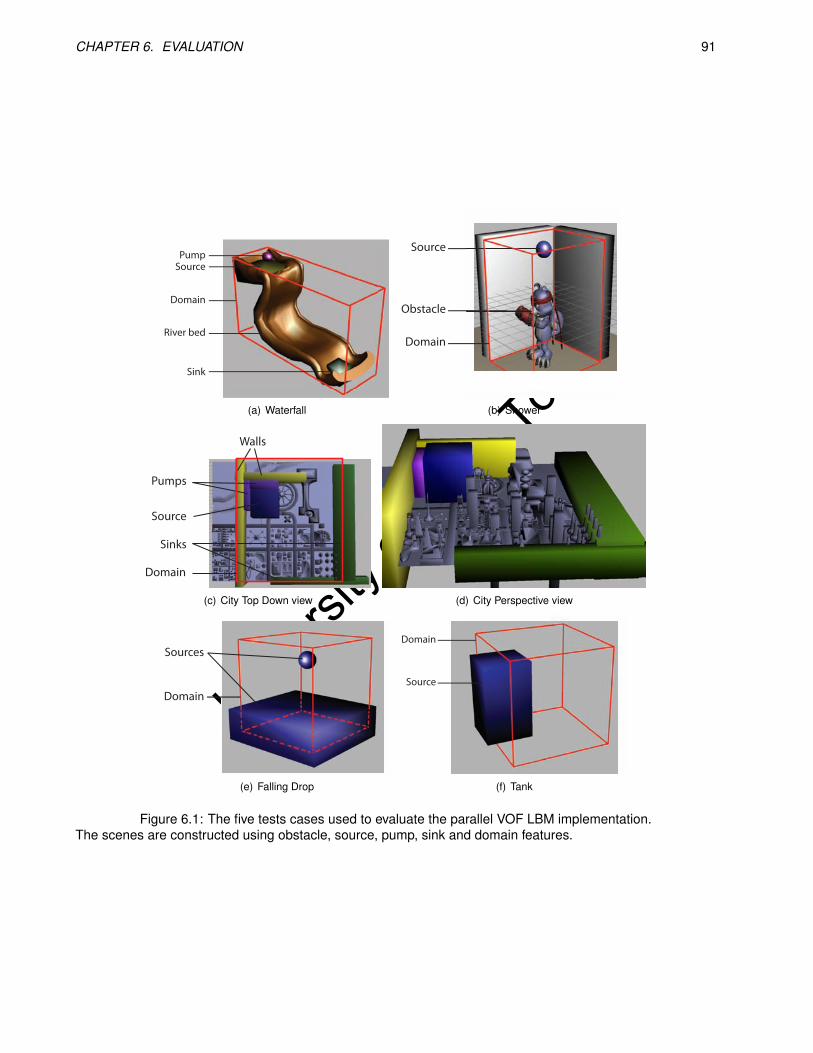
Univers

ity of

Cap

e Tow

n

CHAPTER 6. EVALUATION 91

Pump

Domain

River bed

Sink

Source

(a) Waterfall

Source

Obstacle

Domain

(b) Shower

Walls

Pumps

Source

Sinks

Domain

(c) City Top Down view (d) City Perspective view

Sources

Domain

(e) Falling Drop

Domain

Source

(f) Tank

Figure 6.1: The five tests cases used to evaluate the parallel VOF LBM implementation.The scenes are constructed using obstacle, source, pump, sink and domain features.

Univers

ity of

Cap

e Tow

n


domain, along with two pumps. The block provides the initial wave crashing on the city, while the pumpswill continue to add water to the scene. Two obstacle walls, shown in yellow, are placed to guide the fluidin the correct direction and two sink walls (in green) on the other end of the city are used to absorb thewater. This mimics the scene from The Day After Tomorrow where a city is flooded by a large wave1.

3. Gnomon2 showering in water/mud - Figure 6.1 (b) - depicts a creature being showered with fluid. Natu-rally, the fluid could be anything, such as water or mud. There is only one pump for the scene, a sphereabove the creatures head. The inspiration for this scene is the film Shrek3.

4. Breaking Dam - Figure 6.1 (f) is the standard falling dam from the literature [Thürey, 2003], with a blockof water in the one corner of the domain. The water falls to the bottom of the domain under the effect ofgravity.

5. Water drop falling into a pool - Figure 6.1 (e) is standard falling drop from literature [Pohl and Rüde,2007]. The drop falls into the pool below.

To gain more insight into the algorithm’s performance, the tests were run on two architectures (given in Table5.1) to measure the impact of different technologies on simulation performance. As the cases and architec-tures are different, in the next sections, we use the definitions in Section 2.6.2 as normalized measures of theperformance. The normalized measures can then be compared directly.

The following procedure was used to run each of the test simulations: The scene was specified in Houdiniusing geometry objects. These were processed and grid information was exported to a data file for a singleCPU (it can obviously be exported for multiple CPUs, but due to the time required it was efficient to export justonce). The file was then post-processed to create a grid file for a simulation using N slave processes. Thegrid file was then copied onto the cluster and the simulation run. The wall clock time was recorded from thetime the master process started loading the grid file until it had saved the last frame’s fluid mesh. These timesare used to produce the information and graphs in this chapter.

6.1.1 System scalability

The system scalability was analysed using the definitions for wall clock time, scalability and efficiency providedin Section 2.6.2. It is also important to consider the wall clock time of the simulation with respect to turn aroundtime in a production environment. From this measurement and the above scalability analysis, the highestsimulation scale at which it is practical to simulate fluid can be determined. The scalability is a measure of howwell the simulation is distributed over multiple CPUs.

6.1.2 Load Balancing

The multi-CPU version of the system has two implementations, one with static load balancing and another withdynamic load balancing. As the work load may not be evenly distributed across all the CPUs, the efficiencyis reduced in certain cases. Load balancing seeks to improve the efficiency in these cases. Using the tools

1http://www.imdb.com/title/tt0319262/2A fantastical Digimon character from TV.3www.shrek.com

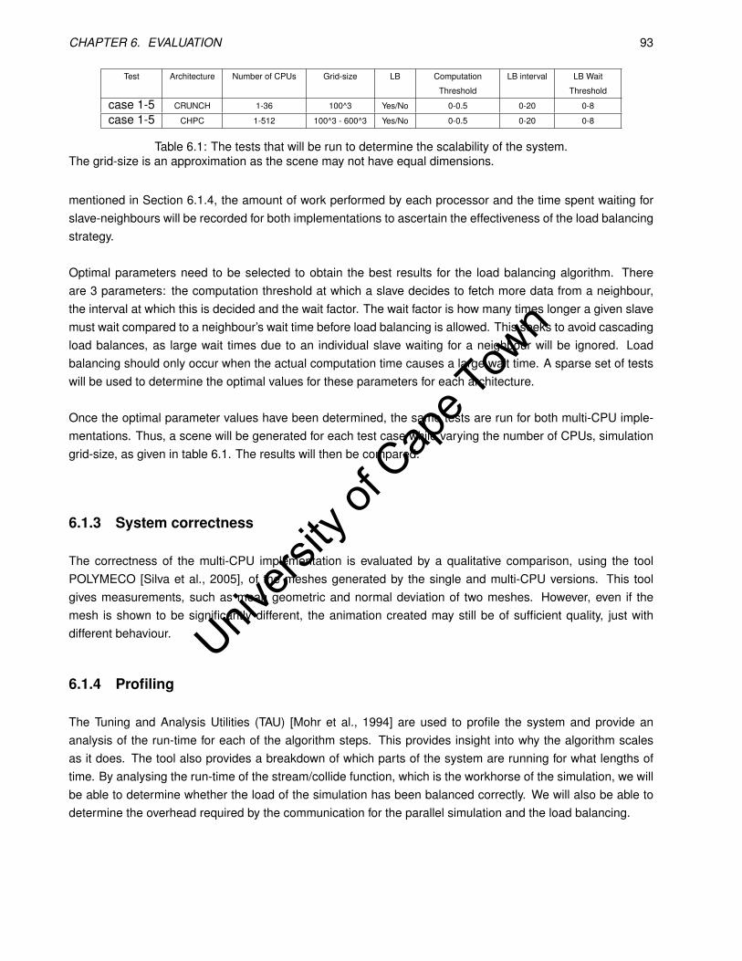
Univers

ity of

Cap

e Tow

n


Test Architecture Number of CPUs Grid-size LB Computation

Threshold

LB interval LB Wait

Threshold

case 1-5 CRUNCH 1-36 100^3 Yes/No 0-0.5 0-20 0-8

case 1-5 CHPC 1-512 100^3 - 600^3 Yes/No 0-0.5 0-20 0-8

Table 6.1: The tests that will be run to determine the scalability of the system.The grid-size is an approximation as the scene may not have equal dimensions.

mentioned in Section 6.1.4, the amount of work performed by each processor and the time spent waiting forslave-neighbours will be recorded for both implementations to ascertain the effectiveness of the load balancingstrategy.

Optimal parameters need to be selected to obtain the best results for the load balancing algorithm. Thereare 3 parameters: the computation threshold at which a slave decides to fetch more data from a neighbour,the interval at which this is decided and the wait factor. The wait factor is how many times longer a given slavemust wait compared to a neighbour’s wait time before load balancing is allowed. This seeks to avoid cascadingload balances, as large wait times due to an individual slave waiting for a neighbour will be ignored. Loadbalancing should only occur when the actual computation time causes a large wait time. A sparse set of testswill be used to determine the optimal values for these parameters for each architecture.

Once the optimal parameter values have been determined, the same tests are run for both multi-CPU imple-mentations. Thus, a scene will be generated for each test case while varying the number of CPUs, simulationgrid-size, as given in table 6.1. The results will then be compared.

6.1.3 System correctness

The correctness of the multi-CPU implementation is evaluated by a qualitative comparison, using the toolPOLYMECO [Silva et al., 2005], of the meshes generated by the single and multi-CPU versions. This toolgives measurements, such as mean geometric and normal deviation of two meshes. However, even if themesh is shown to be significantly different, the animation created may still be of sufficient quality, just withdifferent behaviour.

6.1.4 Profiling

The Tuning and Analysis Utilities (TAU) [Mohr et al., 1994] are used to profile the system and provide ananalysis of the run-time for each of the algorithm steps. This provides insight into why the algorithm scalesas it does. The tool also provides a breakdown of which parts of the system are running for what lengths oftime. By analysing the run-time of the stream/collide function, which is the workhorse of the simulation, we willbe able to determine whether the load of the simulation has been balanced correctly. We will also be able todetermine the overhead required by the communication for the parallel simulation and the load balancing.

Univers

ity of

Cap

e Tow

n


6.2 Results

6.2.1 Animations

All the animations are rendered using Mantra4 from SideFX, with various shaders being used for the differentobjects in the scene. The waterfall is shown in Figure 6.2, with the base of the river using a granite shaderand the water using a basic fluid shader. The granite shader is a black stone, which sparkles in light reflection,and the basic fluid shader allows for the refraction and reflection, properties of fluid. In addition, the fluid hascolour, which is more intense with depth. The fluid in the scene was simulated at a resolution of 500×400×200.

Figure 6.3 shows the drop animation. The grid size for the final simulation was 600 × 600 × 600. The floorof the scene is rendered with a wood shader, the fluid with the basic fluid shader and the walls with plain whiteshading. The drop appears to explode before it hits the surface due to the instabilities of the method.

Figure 6.4 demonstrates the shower animation using a clay shader on the fluid surface and two differentmarble shaders for the walls and floor. A spotlight has been added to the scene to add extra character. Forthis simulation a grid resolution of 480× 720× 480 was used.

The city animation is shown in Figure 6.5 at a resolution of 600× 165× 600. No texture or shader is applied tothe city, but an extra environmental light has been added to introduce ambient occlusion to the rendering.

Figure 6.6 shows the breaking dam, which has a few artifacts, the most significant being the slow drip ofthe fluid down the side of the wall. Since the focus of the thesis is on the efficient production of the meshsurface and not the final look, this has not been further investigated. The scene was simulated at a resolutionof 600× 600× 600.

6.2.2 Parameter tuning

In general, an animator will not know how well the load will be balanced when specifying a scene in which fluidwill be simulated. It is important to be able to choose parameters that will work for multiple scenes with varyingloads. Thus, the optimal value for each of the parameters are evaluated for two distinct test cases: the breakingdam and water drop. The first has with an unbalanced load, while the second is reasonably well balanced load.Evaluating the performance for both cases gives an overall idea of how the parameters influence performanceand values are then chosen to optimise both run-times.

The optimal values for three parameters need to be found, which means running simulations for each pos-sible combination of these parameters. We look at the change of two of the parameters at a time while theother is held constant. In addition, a fixed resolution is used for both cases, 100 × 100 × 100 for the cases onCRUNCH and 200×200×200 for those on CHPC. From the general trends, ranges and values can be selectedfor closer examination. The differences for the two architectures are given.

4www.sidefx.com

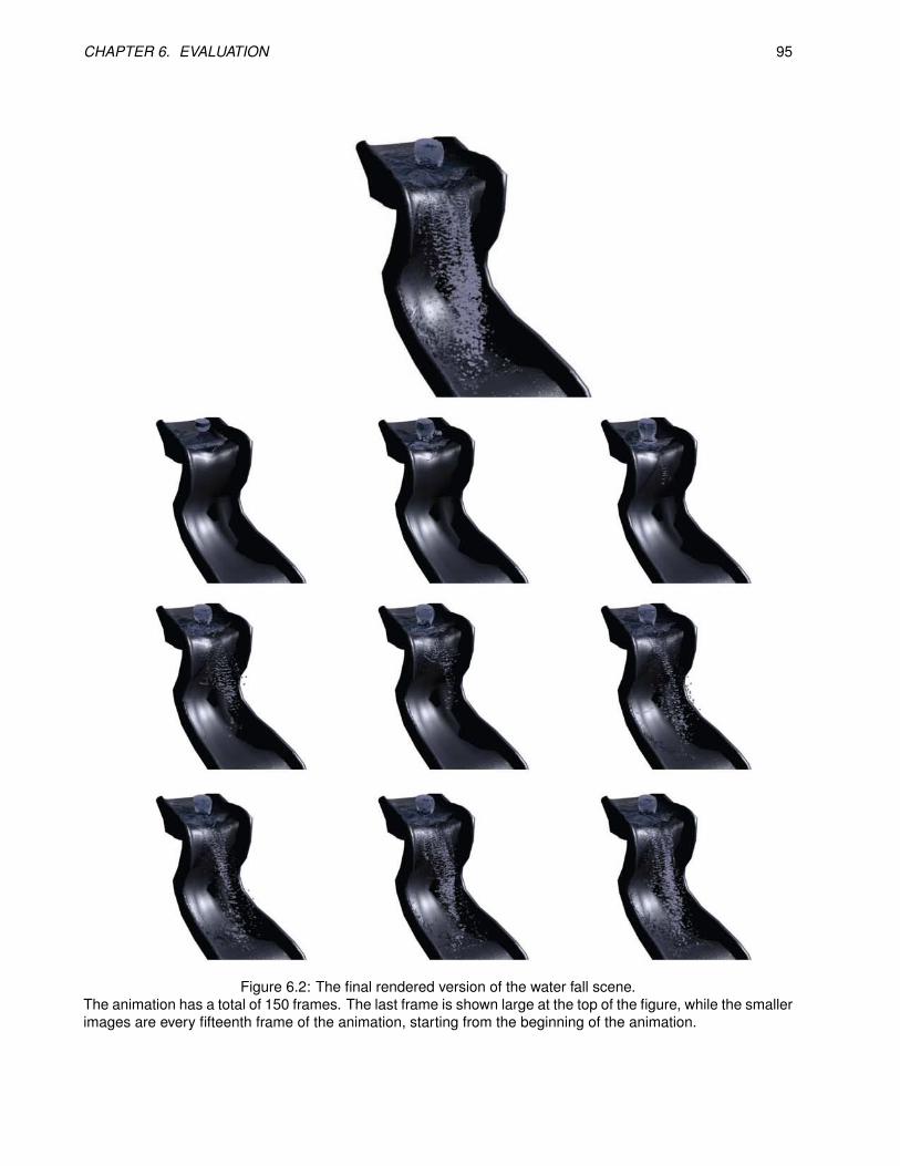
Univers

ity of

Cap

e Tow

n


Figure 6.2: The final rendered version of the water fall scene.The animation has a total of 150 frames. The last frame is shown large at the top of the figure, while the smallerimages are every fifteenth frame of the animation, starting from the beginning of the animation.

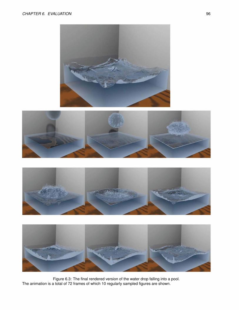
Univers

ity of

Cap

e Tow

n


Figure 6.3: The final rendered version of the water drop falling into a pool.The animation is a total of 72 frames of which 10 regularly sampled figures are shown.

Univers

ity of

Cap

e Tow

n


Figure 6.4: The final rendered version of the shower scene, with fluid rendered as mud.The animation has a total of 150 frames of which 10 regularly sampled figures are shown.

Univers

ity of

Cap

e Tow

n


Figure 6.5: The final rendered version of the wave breaking over the city.The animation is a total of 100 frames, of which 20 are shown.

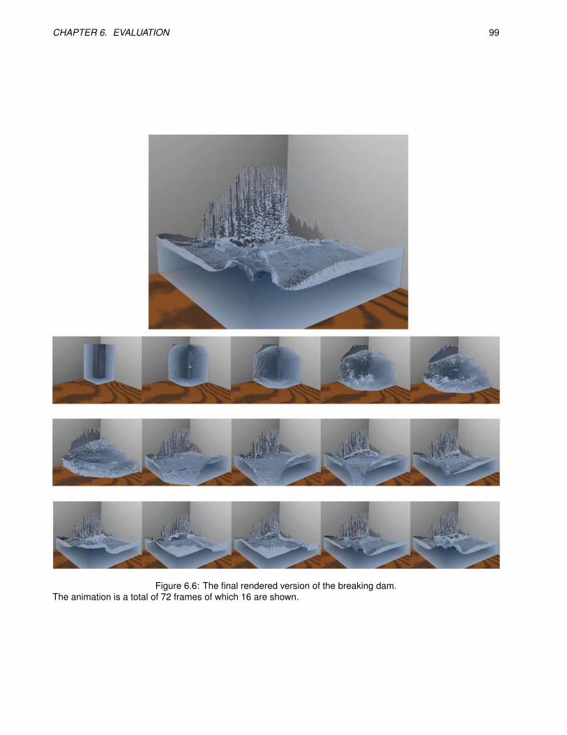
Univers

ity of

Cap

e Tow

n


Figure 6.6: The final rendered version of the breaking dam.The animation is a total of 72 frames of which 16 are shown.

Univers

ity of

Cap

e Tow

n


6.2.2.1 CRUNCH

Figure 6.7 (a) shows the running time for the dam simulation, while varying the computation threshold (CT) ina large range from 0.025-0.375 and the wait factor (WF) from 0.5-3. The load balancing interval is kept at 1. Ingeneral, the running time is invariant under a changing wait factor between 0.5-3 and for computation thresh-olds between 0.025-0.275. For computation thresholds above 0.275, the running time increases dramatically.Figure 6.7 (b) explores a wait factor of 1-6 and a lower computation threshold range of 0.001-0.023. Again,the running time is largely invariant under the wait factor, while the run-time decreases as the computationthreshold increases in the given range, until it reaches the plateau from the previous figure.

Figure 6.7 (c) explores larger wait factors for the dam simulation (1-71), which serve to slow the simulationdown. Smaller wait factors are clearly more optimal. Figure 6.7 (d) shows the times of the simulation as theload balance interval changes (1-10), clearly showing that more frequent load balanced is considerably better.

Figure 6.8 shows similar graphs for the water drop simulation, but for slightly narrower regions of interest,as we want to find parameter values that are suitable for both simulations tested and use the better parameterregions found in the previous tests. The predominant trend with the drop test case is the less load balancingthere is (high load balancing intervals), the better the run-time. No other significant trends were noticed, butperformance changes do not seem as significant.

The invariance of the run-time due to wait factor value is worth discussing. The wait factor, wf , allows aslave to reject a load balance request, which is necessary as the slave may be waiting for another slave tofinish computation. Its value has little effect on the run-time, since slaves that have a high work load will havea very low maximum wait time, tmax, for neighbours. This wait time is multiplied by the wait factor, givingwf tmax. This value is used to decide whether to reject a request that does not make it past the threshold.Since tmax 1, so to will wf tmax 1. The value then becomes inconsequential in the decision processand wf must be very large to influence the decision. Due to slow variance of the run-time with respect to thewait factor and this logic, we choose a value of 1, as this gives good results on the graphs and keeps the loadbalancing as sensitive as possible to changes.

6.2.2.2 CHPC

As seen from the results on the CRUNCH architecture, the LB interval and the computation threshold playthe biggest parts in the simulation times. The LB interval is chosen to be 1 to allow the system to adapt asquickly as possible to changes in the load. It is better if the system is able to make the correct decision morefrequently. Additionally, it was shown that this gave optimal run-times for the unbalanced case of the breakingdam.

With the wait factor and the LB interval fixed, the breaking dam and the falling drop are run for differentcomputation thresholds. Figure 6.9 shows the results. The drop simulation is better with no load balancing atall, while the dam has best run-times when the the load balancing is quite sensitive, using low values for thecomputation threshold. The optimal value for the threshold is not easy to choose, due to this contradiction.

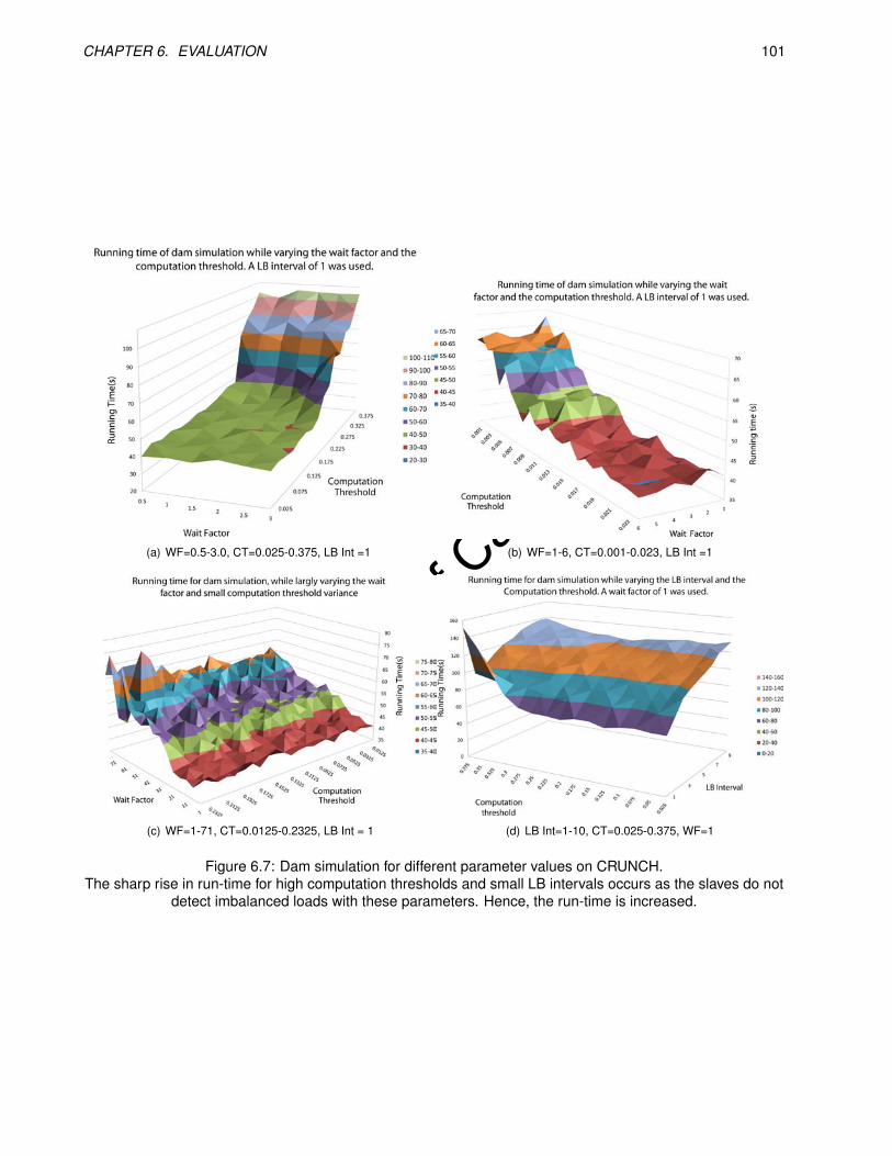
Univers

ity of

Cap

e Tow

n


(a) WF=0.5-3.0, CT=0.025-0.375, LB Int =1 (b) WF=1-6, CT=0.001-0.023, LB Int =1

(c) WF=1-71, CT=0.0125-0.2325, LB Int = 1 (d) LB Int=1-10, CT=0.025-0.375, WF=1

Figure 6.7: Dam simulation for different parameter values on CRUNCH.The sharp rise in run-time for high computation thresholds and small LB intervals occurs as the slaves do not

detect imbalanced loads with these parameters. Hence, the run-time is increased.

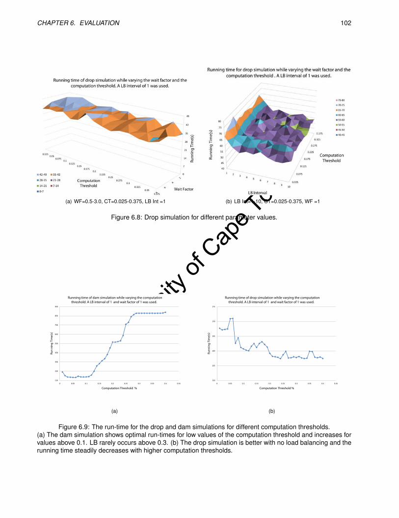
Univers

ity of

Cap

e Tow

n


(a) WF=0.5-3.0, CT=0.025-0.375, LB Int =1 (b) LB Int=1-10, CT=0.025-0.375, WF =1

Figure 6.8: Drop simulation for different parameter values.

150

250

350

450

550

650

750

850

950

0 0.05 0.1 0.15 0.2 0.25 0.3 0.35 0.4 0.45

Run

ning

Tim

e(s)

Computation Threshold %

Running time of dam simulation while varying the computation threshold. A LB interval of 1 and wait factor of 1 was used.

(a)

150

155

160

165

170

175

0 0.05 0.1 0.15 0.2 0.25 0.3 0.35 0.4 0.45

Runn

ing

Tim

e(s)

Computation Threshold %

Running time of drop simulation while varying the computation threshold. A LB interval of 1 and wait factor of 1 was used.

(b)

Figure 6.9: The run-time for the drop and dam simulations for different computation thresholds.(a) The dam simulation shows optimal run-times for low values of the computation threshold and increases forvalues above 0.1. LB rarely occurs above 0.3. (b) The drop simulation is better with no load balancing and therunning time steadily decreases with higher computation thresholds.

Univers

ity of

Cap

e Tow

n


6.2.3 Scalability and Efficiency

Here, the simulations are run for different numbers of CPUs (and the results shown as graphs in Figures 6.10to 6.14). The simulation consists of running 1 master process and N slave processes. Note that for bothCRUNCH and CHPC architectures, each compute node in the cluster has four physical cores and four pro-cesses can be run at a time. Thus, processes are first assigned to the same compute node so communicationtimes are minimised. Processes on the same node make use of the memory based communication of MPIinstead of using the interconnect.

The CHPC is a multi-user system and the test results are effected by the load on the system at the timeof running tests. This yielded variable results for similar runs of test cases. To alleviate this problem, each teston CHPC was run 5 times. The two largest times were discarded and the average of the three remaining timeswas used to produce the graphs. This goes some way to removing the variance due to high loads. CRUNCHhad no such problems.

For the initial scene conditions that are loaded by the master process, there are two different creation methods.The first, for static load balancing, assigns a constant grid width to each of the slave processes. If the length ofthe grid along the x-axis is L and there are N slaves, then each slave gets assigned roughly L

N slices. Thereare adjustments, of course, when L is not perfectly divisible by N . The second, for dynamic load balancing,assigns fluid cells evenly to all slaves. The total number of fluid cells in the scene is counted, let this be F , andthen each slave is given as close to F

N fluid cells as possible. Again the division is not perfect, as entire slicesmust be assigned to slaves.

6.2.3.1 Low Resolutions

The speedup and efficiency results for all the test cases, at a low grid resolution, are given in Figures 6.10 and6.11 respectively. These results are from the CHPC platform, while the partial results for the CRUNCH platformare included in Appendix D.2.The first noticeable information from the graphs is that the simulations runningon the CHPC architecture are markedly better than the CRUNCH architecture. There is little difference in thewall clock time for the single CPU implementation, with the CHPC being slower in both cases. The speedupand efficiency results show that the parallelization is not very efficient when more then 15 CPUs are used. Atthis point, the efficiency falls bellow 70% on CHPC. The dynamic load balancing algorithm performs marginallybetter than static load balancing up to around 17 CPUs, when the speedup is equal and then performs worseafter this point. Although the difference in speedup is negligible overall. The graph of the dynamic load balanc-ing algorithm is smooth, while the static load balancing increases in steps.

The performance difference for the drop and dam simulations with respect to static and dynamic load bal-ancing is not very significant, but the dynamic load balancing is more efficient for lower number of CPUs on theCHPC. On CRUNCH, dynamic load balancing is in general worse, but remains within 5-10% of the efficiencyof the static load balancing. For the CHPC, the performance of static load balancing eventually out performsthe dynamic case, above 17 CPUs. A specific difference is noticed with the dynamic load balancing on thedam simulation, which has a 10% efficiency advantage for lower number of CPUs.

The mud and waterfall simulations are now considered. Both scenes are similar in nature, as water flowsinto part of the scene and fills the scene slowly. The graphs are then quite similar. Both do not scale well

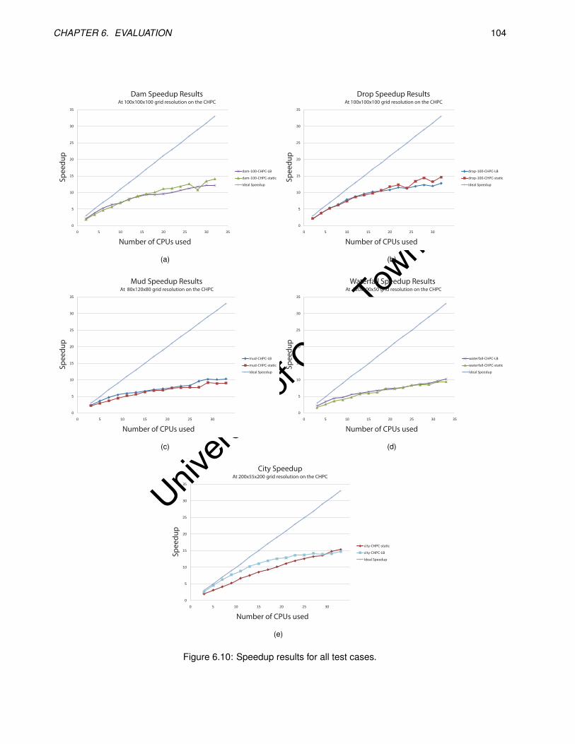
Univers

ity of

Cap

e Tow

n


0

5

10

15

20

25

30

35

0 5 10 15 20 25 30 35

Sp

ee

du

p

Number of CPUs used

Dam Speedup ResultsAt 100x100x100 grid resolution on the CHPC

dam-100-CHPC-LB

dam-100-CHPC-sta c

Ideal Speedup

(a)

0

5

10

15

20

25

30

35

0 5 10 15 20 25 30

Sp

ee

du

p

Number of CPUs used

Drop Speedup ResultsAt 100x100x100 grid resolution on the CHPC

drop-100-CHPC-LB

drop-100-CHPC-sta c

Ideal Speedup

(b)

0

5

10

15

20

25

30

35

0 5 10 15 20 25 30

Sp

ee

du

p

Number of CPUs used

Mud Speedup Results At 80x120x80 grid resolution on the CHPC

mud-CHPC-LB

mud-CHPC-sta c

Ideal Speedup

(c)

0

5

10

15

20

25

30

35

0 5 10 15 20 25 30 35

Sp

ee

du

p

Number of CPUs used

Waterfall Speedup Results At 120x100x50 grid resolution on the CHPC

waterfall-CHPC-LB

waterfall-CHPC-sta c

Ideal Speedup

(d)

0

5

10

15

20

25

30

35

0 5 10 15 20 25 30

Sp

ee

du

p

Number of CPUs used

City Speedup At 200x55x200 grid resolution on the CHPC

city-CHPC-sta c

city-CHPC-LB

Ideal Speedup

(e)

Figure 6.10: Speedup results for all test cases.

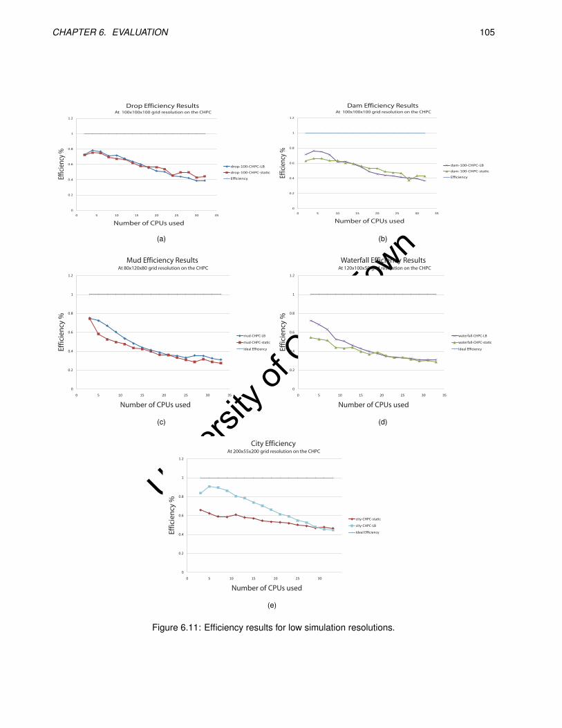
Univers

ity of

Cap

e Tow

n


0

0.2

0.4

0.6

0.8

1

1.2

0 5 10 15 20 25 30 35

Effic

ienc

y %

Number of CPUs used

Drop Efficiency ResultsAt 100x100x100 grid resolution on the CHPC

drop-100-CHPC-LB

drop-100-CHPC-sta c

Efficiency

(a)

0

0.2

0.4

0.6

0.8

1

1.2

0 5 10 15 20 25 30 35

Effic

ienc

y %

Number of CPUs used

Dam Efficiency ResultsAt 100x100x100 grid resolution on the CHPC

dam-100-CHPC-LB

dam-100-CHPC-sta c

Efficiency

(b)

0

0.2

0.4

0.6

0.8

1

1.2

0 5 10 15 20 25 30 35

Eff

icie

ncy

%

Number of CPUs used

Mud Efficiency Results At 80x120x80 grid resolution on the CHPC

mud-CHPC-LB

mud-CHPC-sta c

Ideal Efficiency

(c)

0

0.2

0.4

0.6

0.8

1

1.2

0 5 10 15 20 25 30 35

Eff

icie

ncy

%

Number of CPUs used

Waterfall Efficiency Results At 120x100x50 grid resolution on the CHPC

waterfall-CHPC-LB


Ideal Efficiency

(d)

0

0.2

0.4

0.6

0.8

1

1.2

0 5 10 15 20 25 30

Eff

icie

ncy

%

Number of CPUs used

City Efficiency At 200x55x200 grid resolution on the CHPC

city-CHPC-sta c

city-CHPC-LB

Ideal Efficiency

(e)

Figure 6.11: Efficiency results for low simulation resolutions.

Univers

ity of

Cap

e Tow

n


above 10 CPUs. This can be seen most easily in the efficiency graph, which shows a drop of efficiency tobelow 50%. The performance of the static and dynamic load balancing are also both very similar, but dynamicload balancing gives about 3-20% efficiency improvement in the range of 5-12CPUs.

The city simulation results show a much larger performance difference between the dynamic and static loadbalancing. The dynamic load balancing achieves an efficiency above 90% for 5 CPUs. The crossover point forthe static and dynamic cases is at 32 CPUs.

The wall clock times (see Appendix D.2) for all of the simulations are good and the simulations can all begenerated in under 2 minutes with less then 10 CPUs. Another notable feature, present on some of the effi-ciency graphs for the CHPC, is that the efficiency increases from one node to two.

6.2.3.2 Medium resolutions

Here, we present the results from running the simulations at medium resolutions. Due to the memory limita-tions on the crunch architecture, the tests were only run on the CHPC. The wall clock times are included inthe Appendix D.2, Figure D.7, as they are similar to the previous wall clock graphs and the speedup/efficiencygraphs provide greater insight. In general, the wall clock times show a fast reduction in time when using up to10-15 CPUs and then far less improved performance for higher CPUs.

The speedup and efficiency results for all the test cases, at a medium grid resolution, are given in Figures6.15 and 6.14 respectively. The graphs of the drop and dam show some of the same characteristics as theirlow resolution counterparts. The performance stepping that is present for the static load balancing case is alsopresent in the medium resolution cases. The dynamic load balancing shows a smooth graph, indicating thatthe load is more evenly balanced. However, again there is a crossover point where the static load balancinghas better performance. For the drop simulation, this occurs at 20 CPUs and for the dam simulation between15-20 CPUs (most easily seen on the efficiency graph). There is the same increase in efficiency from 2 to 10CPUs and then a subsequent decrease.

The waterfall and mud results also exhibit similar properties. In general, poor scaling beyond 10 CPUs is ob-served and slightly better performance for dynamic load balancing until a crossover point. The city simulationshows a far larger efficiency gain with the dynamic load balancing, but ultimately poor scaling beyond 30 CPUs.

When comparing the low resolution results against the medium resolution results, the drop and dam simu-lations evidence better efficiency and, therefore, better scaling. The mud and water simulations have similarefficiency results and the city poorer results.

6.2.3.3 High Resolutions

The speedup and efficiency results for all the test cases, at a high grid resolution, are given in Figures 6.10and 6.11 respectively. As the memory required to run a simulation on a single CPU is prohibitively large, anestimate for the single CPU run-time is obtained by fitting a power regression line to the static load balancingdata. This value is then used in the calculation of the speedup and efficiency.

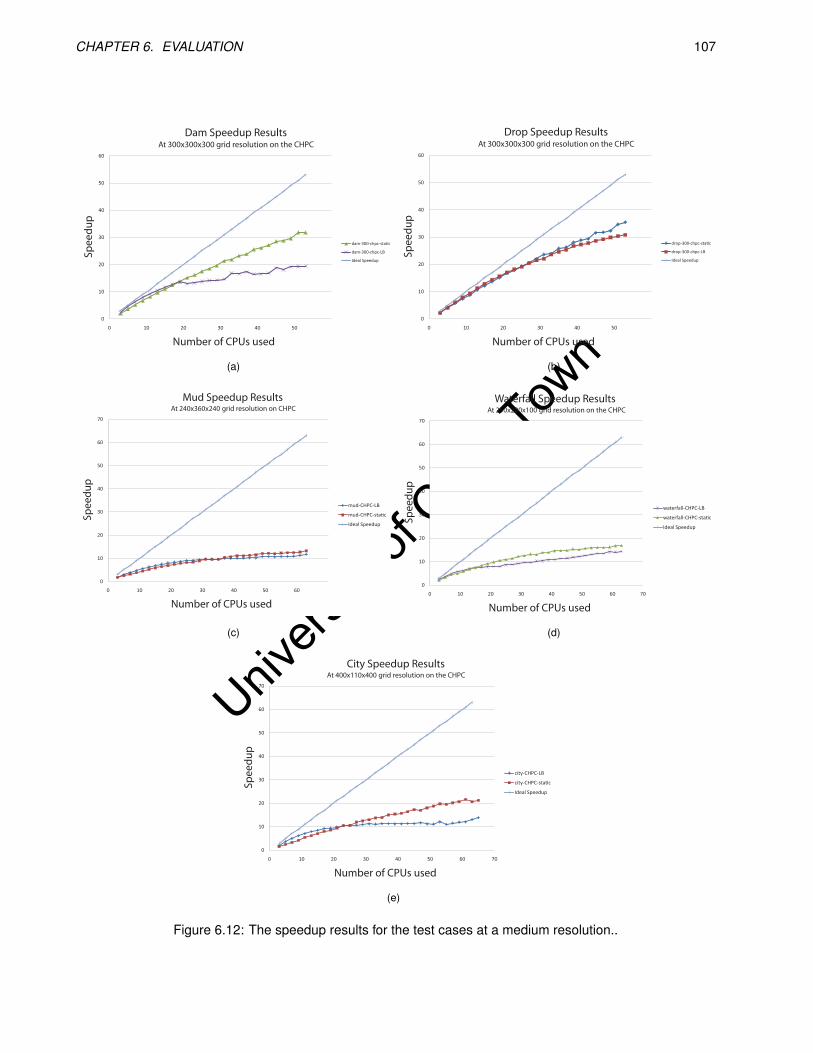
Univers

ity of

Cap

e Tow

n


0

10

20

30

40

50

60

0 10 20 30 40 50

Sp

ee

du

p

Number of CPUs used

Dam Speedup ResultsAt 300x300x300 grid resolution on the CHPC

dam-300-chpc-sta c

dam-300-chpc-LB

Ideal Speedup

(a)

0

10

20

30

40

50

60

0 10 20 30 40 50

Sp

ee

du

p

Number of CPUs used

Drop Speedup ResultsAt 300x300x300 grid resolution on the CHPC

drop-300-chpc-sta c

drop-300-chpc-LB

Ideal Speedup

(b)

0

10

20

30

40

50

60

70

0 10 20 30 40 50 60

Sp

ee

du

p

Number of CPUs used

Mud Speedup Results At 240x360x240 grid resolution on CHPC

mud-CHPC-LB

mud-CHPC-sta c

Ideal Speedup

(c)

0

10

20

30

40

50

60

70

0 10 20 30 40 50 60 70

Sp

ee

du

p

Number of CPUs used


waterfall-CHPC-LB


Ideal Speedup

(d)

0

10

20

30

40

50

60

70

0 10 20 30 40 50 60 70

Sp

ee

du

p

Number of CPUs used

City Speedup Results At 400x110x400 grid resolution on the CHPC

city-CHPC-LB

city-CHPC-sta c

Ideal Speedup

(e)

Figure 6.12: The speedup results for the test cases at a medium resolution..

Univers

ity of

Cap

e Tow

n


0

0.2

0.4

0.6

0.8

1

1.2

0 10 20 30 40 50 60

Eff

icie

ncy

%

Number of CPUs used

Dam Efficiency ResultsAt 300x300x300 grid resolution on the CHPC

dam-300-stat

dam-300-LB

Ideal Efficiency

(a)

0

0.2

0.4

0.6

0.8

1

1.2

0 10 20 30 40 50 60

Eff

icie

ncy

%

Number of CPUs used

Drop Efficiency ResultsAt 300x300x300 grid resolution on the CHPC

Ideal Efficiency

drop-300-stat

drop-300-LB

(b)

0

0.2

0.4

0.6

0.8

1

1.2

0 10 20 30 40 50 60 70

Eff

icie

ncy

%

Number of CPUs used


mud-CHPC-LB

mud-CHPC-sta c

Ideal Efficiency

(c)

0

0.2

0.4

0.6

0.8

1

1.2

0 10 20 30 40 50 60

Eff

icie

ncy

%

Number of CPUs used


waterfall-CHPC-LB


Ideal Efficiency

(d)

0

0.2

0.4

0.6

0.8

1

1.2

0 10 20 30 40 50 60

Eff

icie

ncy

%

Number of CPUs used

City Efficiency Results At 400x110x400 grid resolution on the CHPC

city-CHPC-sta c

city-CHPC-LB

Ideal Efficiency

(e)

Figure 6.13: The efficiency results for the test cases at a medium resolution.

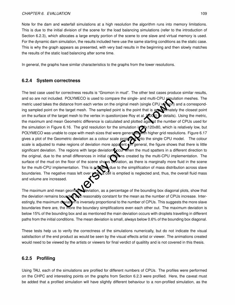
Univers

ity of

Cap

e Tow

n


Note for the dam and waterfall simulations at a high resolution the algorithm runs into memory limitations.This is due to the initial division of the scene for the load balancing simulations (refer to the introduction ofSection 6.2.3), which allocates a large empty portion of the scene to one slave and virtual memory is used.For the dynamic dam simulation, the results included here use the same starting conditions as the static case.This is why the graph appears as presented, with very bad results in the beginning and then slowly matchesthe results of the static load balancing after some time.

In general, the graphs have similar characteristics to the graphs from the lower resolutions.

6.2.4 System correctness

The test case used for correctness results is “Gnomon in mud”. The other test cases produce similar results,and so are not included. POLYMECO is used to compare the single- and multi-CPU simulation meshes. Themetric used takes the distance from each vertex on the original mesh (single CPU version) and a correspond-ing sampled point on the target mesh. The sampled point is the point that is approximately the closest pointon the surface of the target mesh to the vertex in question(see Roy et al. [2004] for details). Using the metric,the maximum and mean Geometric difference is calculated and plotted against the number of CPUs used forthe simulation in Figure 6.16. The grid resolution for the simulation is 80x120x80, which is relatively low, butPOLYMECO was unable to cope with mesh sizes that were generated with higher grid resolutions. Figure 6.17gives a plot of the Geometric deviation as a colour scale projected onto the single CPU model. The colourscale is adjusted to make regions of deviation more apparent. In general, the figure shows that there is littlesignificant deviation. The regions with large deviation occur when the mud spatters in a different direction tothe original, due to the small differences in initial conditions created by the multi-CPU implementation. Thesurface of the mud on the floor of the scene shows deviation, as there is marginally more fluid in the scenefor the multi-CPU implementation. This is probably due to the simplification of mass distribution across slaveboundaries. The negative mass left over when a cell is emptied is neglected and, thus, the overall fluid massand volume are increased.

The maximum and mean geometric deviation, as a percentage of the bounding box diagonal plots, show thatthe deviation remains bounded and reasonably constant for the mean as the number of CPUs increase. Inter-estingly, the maximum deviation is inversely proportional to the number of CPUs. This suggests the more slaveboundaries there are, the more the boundary simplifications even each other out. The maximum deviation isbelow 15% of the bounding box and as mentioned the main deviation occurs with droplets travelling in differentpaths from the initial conditions. The mean deviation is small, always below 0.6% of the bounding box diagonal.

These tests help us to verify the correctness of the simulations numerically, but do not indicate the visualsatisfaction of the end product as would be seen by the visual effects artist or viewer. The animations createdwould need to be viewed by the artists or viewers for final verdict of qualitity and is not covered in this thesis.

6.2.5 Profiling

Using TAU, each of the simulations are profiled for different numbers of CPUs. The profiles were performedon the CHPC and interesting points on the graphs from Section 6.2.3 were profiled. Here, the caveat mustbe added that a profiled simulation will have slightly different behaviour to a non-profiled simulation, as the

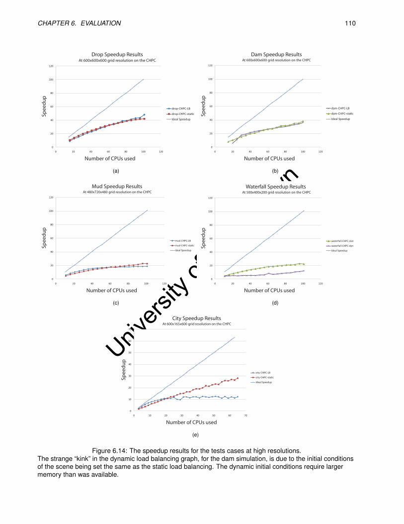
Univers

ity of

Cap

e Tow

n


0

20

40

60

80

100

120

0 20 40 60 80 100 120

Sp

ee

du

p

Number of CPUs used

Drop Speedup Results At 600x600x600 grid resolution on the CHPC

drop-CHPC-LB

drop-CHPC-sta c

Ideal Speedup

(a)

0

20

40

60

80

100

120

0 20 40 60 80 100 120

Sp

ee

du

p

Number of CPUs used

Dam Speedup Results At 600x600x600 grid resolution on the CHPC

dam-CHPC-LB

dam-CHPC-sta c

Ideal Speedup

(b)

0

20

40

60

80

100

120

0 20 40 60 80 100 120

Sp

ee

du

p

Number of CPUs used

Mud Speedup Results At 480x720x480 grid resolution on the CHPC

mud-CHPC-LB

mud-CHPC-sta c

Ideal Speedup

(c)

0

20

40

60

80

100

120

0 20 40 60 80 100 120

Sp

ee

du

p

Number of CPUs used


waterfall-CHPC-stat

waterfall-CHPC-dyn

Ideal Speedup

(d)

0

10

20

30

40

50

60

70

0 10 20 30 40 50 60 70

Sp

ee

du

p

Number of CPUs used

City Speedup ResultsAt 600x165x600 grid resolution on the CHPC

city-CHPC-LB

city-CHPC-sta c

Ideal Speedup

(e)

Figure 6.14: The speedup results for the tests cases at high resolutions.The strange “kink” in the dynamic load balancing graph, for the dam simulation, is due to the initial conditionsof the scene being set the same as the static load balancing. The dynamic initial conditions require largermemory than was available.

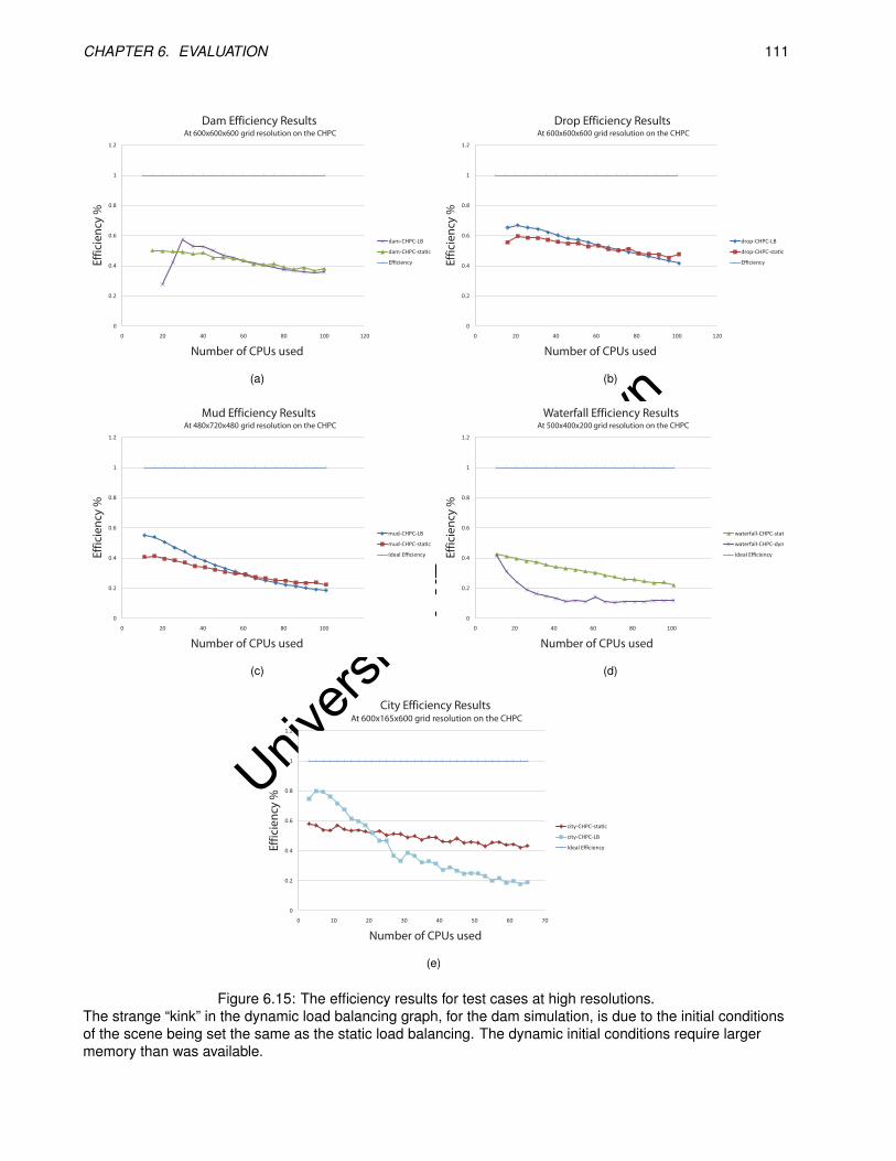
Univers

ity of

Cap

e Tow

n


0

0.2

0.4

0.6

0.8

1

1.2

0 20 40 60 80 100 120

Eff

icie

ncy

%

Number of CPUs used

Dam Efficiency Results At 600x600x600 grid resolution on the CHPC

dam-CHPC-LB

dam-CHPC-sta c

Efficiency

(a)

0

0.2

0.4

0.6

0.8

1

1.2

0 20 40 60 80 100 120

Eff

icie

ncy

%

Number of CPUs used

Drop Efficiency Results At 600x600x600 grid resolution on the CHPC

drop-CHPC-LB

drop-CHPC-sta c

Efficiency

(b)

0

0.2

0.4

0.6

0.8

1

1.2

0 20 40 60 80 100

Eff

icie

ncy

%

Number of CPUs used


mud-CHPC-LB

mud-CHPC-sta c

Ideal Efficiency

(c)

0

0.2

0.4

0.6

0.8

1

1.2

0 20 40 60 80 100

Eff

icie

ncy

%

Number of CPUs used


waterfall-CHPC-stat

waterfall-CHPC-dyn

Ideal Efficiency

(d)

0

0.2

0.4

0.6

0.8

1

1.2

0 10 20 30 40 50 60 70

Eff

icie

ncy

%

Number of CPUs used

City Efficiency ResultsAt 600x165x600 grid resolution on the CHPC

city-CHPC-sta c

city-CHPC-LB

Ideal Efficiency

(e)

Figure 6.15: The efficiency results for test cases at high resolutions.The strange “kink” in the dynamic load balancing graph, for the dam simulation, is due to the initial conditionsof the scene being set the same as the static load balancing. The dynamic initial conditions require largermemory than was available.

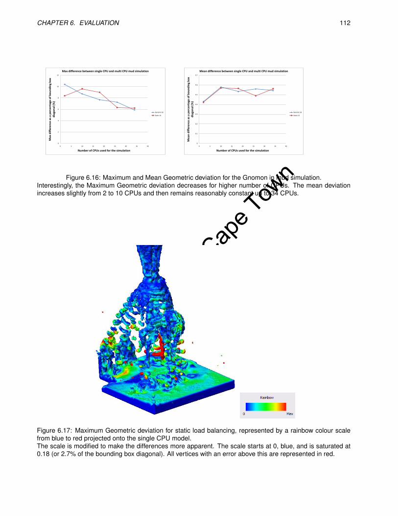
Univers

ity of

Cap

e Tow

n


0

2

4

6

8

10

12

0 5 10 15 20 25 30 35 40

Max

dif

fere

nce

as

a p

erc

en

tage

of

bo

un

din

g b

ox

dia

gon

al (

%)

Number of CPUs used for the simulation

Max difference between single CPU and multi CPU mud simulation

Dynamic LB

Static LB

0

0.1

0.2

0.3

0.4

0.5

0.6

0.7

0 5 10 15 20 25 30 35 40

Me

an d

iffe

ren

ce a

s a

pe

rce

nta

ge o

f b

ou

nd

ing

bo

x d

iago

nal

(%

)

Number of CPUs used for the simulation

Mean difference between single CPU and multi CPU mud simulation

Dynamic LB

Static LB

Figure 6.16: Maximum and Mean Geometric deviation for the Gnomon in mud simulation.Interestingly, the Maximum Geometric deviation decreases for higher number of CPUs. The mean deviationincreases slightly from 2 to 10 CPUs and then remains reasonably constant up to 34 CPUs.

Figure 6.17: Maximum Geometric deviation for static load balancing, represented by a rainbow colour scalefrom blue to red projected onto the single CPU model.The scale is modified to make the differences more apparent. The scale starts at 0, blue, and is saturated at0.18 (or 2.7% of the bounding box diagonal). All vertices with an error above this are represented in red.

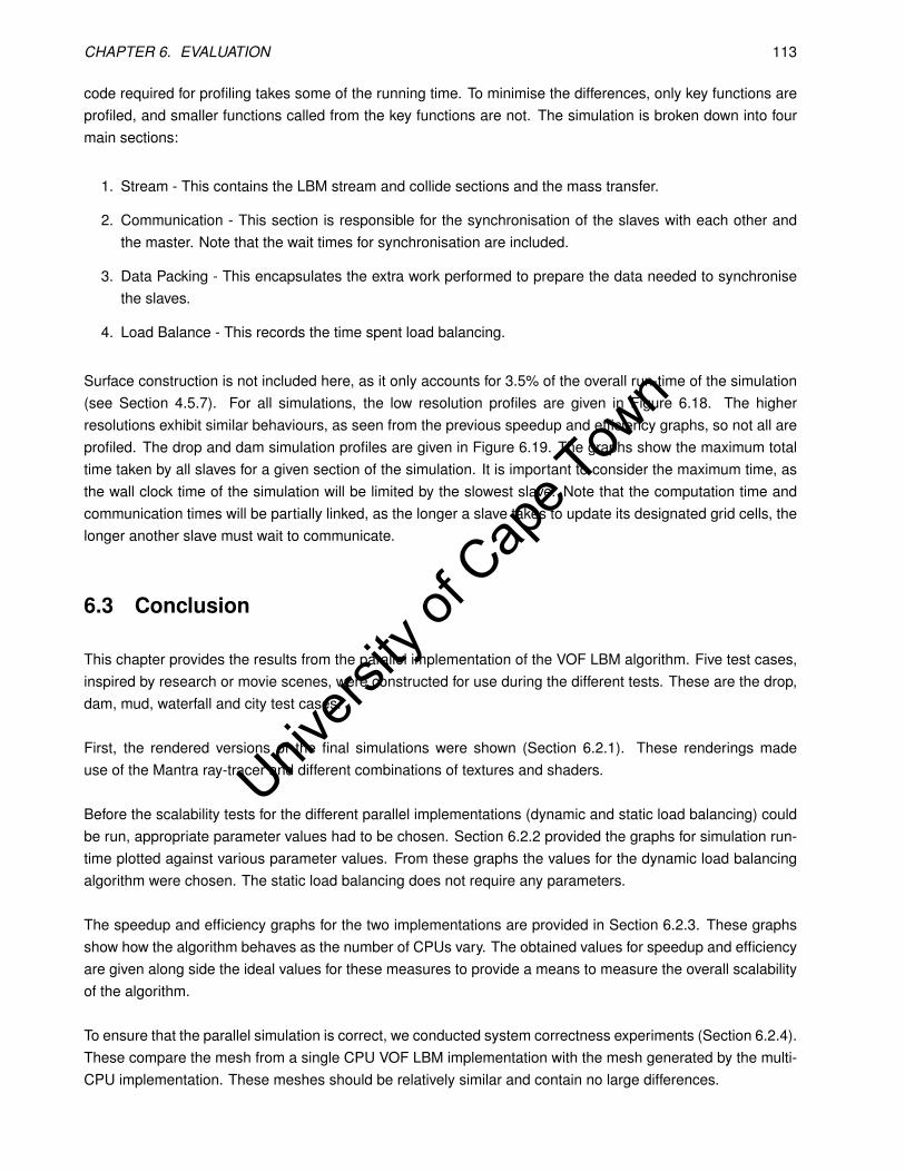
Univers

ity of

Cap

e Tow

n


code required for profiling takes some of the running time. To minimise the differences, only key functions areprofiled, and smaller functions called from the key functions are not. The simulation is broken down into fourmain sections:

1. Stream - This contains the LBM stream and collide sections and the mass transfer.

2. Communication - This section is responsible for the synchronisation of the slaves with each other andthe master. Note that the wait times for synchronisation are included.

3. Data Packing - This encapsulates the extra work performed to prepare the data needed to synchronisethe slaves.

4. Load Balance - This records the time spent load balancing.

Surface construction is not included here, as it only accounts for 3.5% of the overall run-time of the simulation(see Section 4.5.7). For all simulations, the low resolution profiles are given in Figure 6.18. The higherresolutions exhibit similar behaviours, as seen from the previous speedup and efficiency graphs, so not all areprofiled. The drop and dam simulation profiles are given in Figure 6.19. The graphs show the maximum totaltime taken by all slaves for a given section of the simulation. It is important to consider the maximum time, asthe wall clock time of the simulation will be limited by the slowest slave. Note that the computation time andcommunication times will be partially linked, as the longer a slave takes to update its designated grid cells, thelonger another slave must wait to communicate.

6.3 Conclusion

This chapter provides the results from the parallel implementation of the VOF LBM algorithm. Five test cases,inspired by research or movie scenes, were constructed for use during the different tests. These are the drop,dam, mud, waterfall and city test cases.

First, the rendered versions of the final simulations were shown (Section 6.2.1). These renderings madeuse of the Mantra ray-tracer and different combinations of textures and shaders.

Before the scalability tests for the different parallel implementations (dynamic and static load balancing) couldbe run, appropriate parameter values had to be chosen. Section 6.2.2 provided the graphs for simulation run-time plotted against various parameter values. From these graphs the values for the dynamic load balancingalgorithm were chosen. The static load balancing does not require any parameters.

The speedup and efficiency graphs for the two implementations are provided in Section 6.2.3. These graphsshow how the algorithm behaves as the number of CPUs vary. The obtained values for speedup and efficiencyare given along side the ideal values for these measures to provide a means to measure the overall scalabilityof the algorithm.

To ensure that the parallel simulation is correct, we conducted system correctness experiments (Section 6.2.4).These compare the mesh from a single CPU VOF LBM implementation with the mesh generated by the multi-CPU implementation. These meshes should be relatively similar and contain no large differences.

Univers

ity of

Cap

e Tow

n


0.00E+00

1.00E+04

2.00E+04

3.00E+04

4.00E+04

5.00E+04

6.00E+04

7.00E+04

8.00E+04

9.00E+04

1.00E+05

Stream Communication Data Packing Load balance

Tim

e (

mir

co s

eco

nd

s)

Program section

Profiled maximum times of program segmants for dam simulation at 100x100x100 grid resolution for 4 and 26 slaves

slaves=4,stat

slaves=4,dyn

slaves=26,stat

slaves=26,dyn

(a)

0.00E+00

2.00E+04

4.00E+04

6.00E+04

8.00E+04

1.00E+05

1.20E+05

1.40E+05


Tim

e (

mir

co s

eco

nd

s)

Program section

Profiled maximum times of program segmants for drop simulation at 100x100x100 grid resolution for 4 and 26 slaves

slaves=4,stat

slaves=4,dyn

slaves=26,stat

slaves=26,dyn

(b)

0.00E+00

1.00E+04

2.00E+04

3.00E+04

4.00E+04

5.00E+04

6.00E+04

7.00E+04

8.00E+04


Tim

e (

mir

co s

eco

nd

s)

Program section

Profiled maximum times of program segmants for mud simulation at 80x120x80 grid resolution for 6 and 26 slaves

slaves=6,stat

slaves=6,dyn

slaves=26,stat

slaves=26,dyn

(c)

0.00E+00

5.00E+03

1.00E+04

1.50E+04

2.00E+04

2.50E+04

3.00E+04

3.50E+04

4.00E+04

4.50E+04

5.00E+04


Tim

e (

mir

co s

eco

nd

s)

Program section

Profiled maximum times of program segmants for waterfall simulation at 120x100x50 grid resolution for 6 and 26 slaves

slaves=6,stat

slaves=6,dyn

slaves=26,stat

slaves=26,dyn

(d)

0.00E+00

2.00E+04

4.00E+04

6.00E+04

8.00E+04

1.00E+05

1.20E+05


Tim

e (

mir

co s

eco

nd

s)

Program section

Profiled maximum times of program segmants for city simulation at 200x55x200 grid resolution for 15 and 32 slaves

slaves=6,stat

slaves=6,dyn

slaves=26,stat

slaves=26,dyn

(e)

Figure 6.18: Profiling of simulations at low resolutions.The four major sections of the simulation have been profiled and are indicated on the graphs.

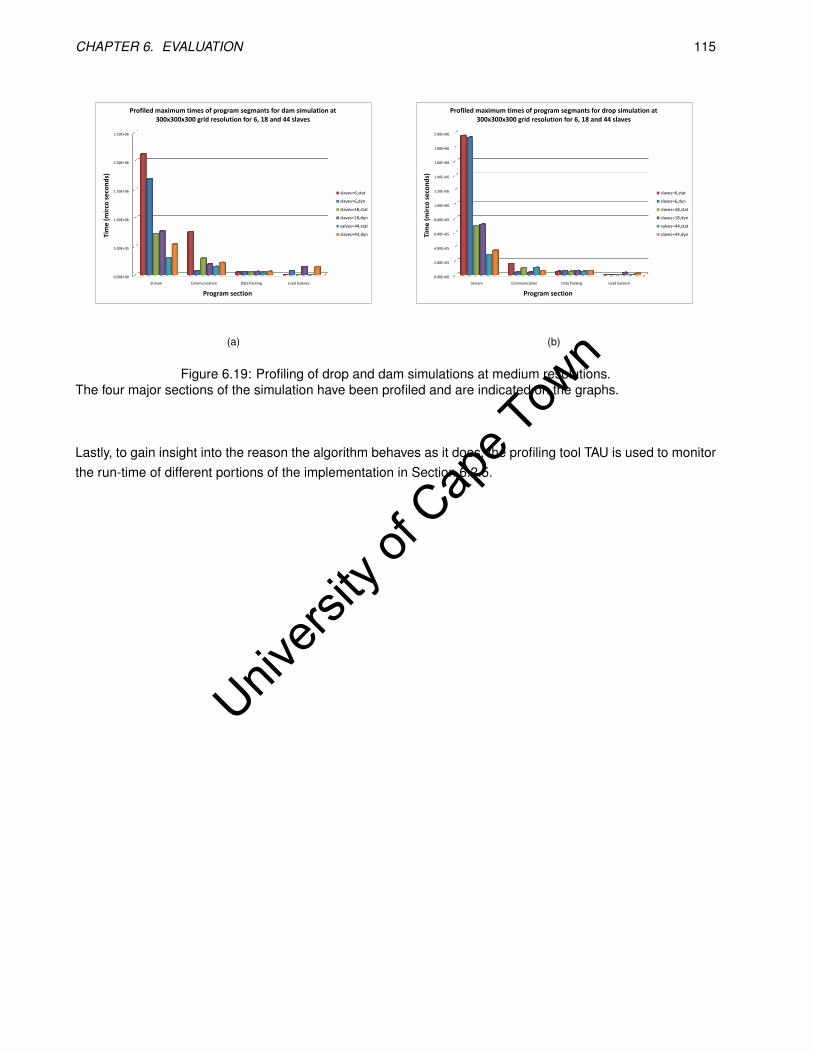
Univers

ity of

Cap

e Tow

n


0.00E+00

5.00E+05

1.00E+06

1.50E+06

2.00E+06

2.50E+06


Tim

e (

mir

co s

eco

nd

s)

Program section

Profiled maximum times of program segmants for dam simulation at 300x300x300 grid resolution for 6, 18 and 44 slaves

slaves=6,stat

slaves=6,dyn

slaves=18,stat

slaves=18,dyn

salves=44,stat

slaves=44,dyn

(a)

0.00E+00

2.00E+05

4.00E+05

6.00E+05

8.00E+05

1.00E+06

1.20E+06

1.40E+06

1.60E+06

1.80E+06

2.00E+06


Tim

e (

mir

co s

eco

nd

s)

Program section

Profiled maximum times of program segmants for drop simulation at 300x300x300 grid resolution for 6, 18 and 44 slaves

slaves=6,stat

slaves=6,dyn

slaves=18,stat

slaves=18,dyn

salves=44,stat

slaves=44,dyn

(b)

Figure 6.19: Profiling of drop and dam simulations at medium resolutions.The four major sections of the simulation have been profiled and are indicated on the graphs.

Lastly, to gain insight into the reason the algorithm behaves as it does, the profiling tool TAU is used to monitorthe run-time of different portions of the implementation in Section 6.2.5.

Univers

ity of

Cap

e Tow

n

Chapter 7

Discussion

Here, we interpret the results presented in Chapter 6. We begin with comments on the general production ofthe final animations from start to finish (in Section 7.2), that is from scene creation through to the renderingof the final animation. The parameter selection for dynamic load balancing is discussed next in Section 7.3.Examination of the scalability and efficiency results are given in Section 7.4 and, lastly, we provide recommen-dations for architecture choices and feasible simulation scales.

7.1 Implementation and development

One important point to emphasize is that a parallel simulation is a very complex system, with different inter-acting parts and numerous algorithm synchronicities. With greater levels of complexity added by the parallelimplementation and load balancing, it becomes increasingly difficult to manage “a stable release” version ofthe code. Here, the definition of “stable” is the same as that used in software life cycle development and differs,of course, from the stability of the algorithm from a numerical point of view. These two things are often linked.Essentially, the “stable release” version would be one which behaves as expected without any bugs. To verifythis, multiple test cases are needed. For the parallel simulation, this means the full spectrum of simulationsused in this thesis. These need to be run for different numbers of CPUs and parameter values. The output ofthe simulations then need to be verified.

This testing process has been performed for this thesis, but further testing is still warranted. The requiredoutcome definition, namely “something that looks visually appealing”, also causes problems with the testingand analysis process. For example, one bug that was found, was that the parallel version of the implementationproduced more fluid for greater numbers of CPUs. This was due to an efficiency optimisation, where somecells were not informed of cell states for neighbouring cells on a slave-neighbour. The effects of this bug werenot noticeable until the mud and waterfall tests cases were analysed for correctness using POLYMECO, asthey appeared correct when rendered. Of course, this would skew the scalability results, so the bug neededto be fixed. This example illustrates the need for testing almost every change to the code base, to make surethat everything is running correctly.

More problems arise when a bug manifests in the parallel implementation, as a cluster environment is not

116

Univers

ity of

Cap

e Tow

n

CHAPTER 7. DISCUSSION 117

easy to debug. The changing workload division of the dynamic load balancing also complicates matters. Onesolution to this problem is a stricter definition of the required outcome, to more closely match physical con-straints. An example of such a constraint is the conservation of mass. In this case, after each step of thealgorithm (or even some sub-steps), mass could be compared against the previous step’s mass. The masternode in the simulation would have to collect the results from the slaves to determine that the global massremains constant. Other approaches, such as monitoring each of the distribution functions, could be taken.

Ideally, two implementations should be created, a debug version and a release version. The debug versionshould contain both sanity checks and physical constraint checks, perhaps in the form of assertions. Thisversion could then be run in an automated fashion and when a violation occurs, a violation notification couldbe sent.

It is important to mention here the nature of the LBM. It is a scheme that eventually arrives at fluid behaviourconsistent with the Navier-Stokes equations. It is not a direct numerical solution to these equations. The proofof equivalence makes use of a number of assumptions (Appendix B). The correctness of these assumptionscan be strongly argued, but nevertheless the scheme is somewhat decoupled from the exact Navier-Stokesequations. The origin of the LBM was also in part based on trial and error (Section 2.4.1.2). Researchersfound what worked and used that. Indeed, the stability analysis that has been researched (Section 3.2.3) isnot complete and the algorithm is not fully understood. This makes it harder to be exactly sure what physicalinteractions should be taking place and, thus, harder to ensure physical correctness in the face of inadvertantbugs.

The same statement can be made for the VOF method of Thurey et al. [2006]. It is not fully defined andthe relation to physical effects are “rule of thumb” methods rather then direct physical equations. Nonethelessthis surface method lends itself well to the LBM and because of its simplicity, constraint checking can be addedeasily.

A strong advantage of the LBM method, is that all effects are localised to a certain grid region. For exam-ple, if an incorrect value were to occur in one cell, causing corruption in the physical properties, then it wouldtake time to propagate to other cells. It is easy to locate such occurrences and the exact error. The simple dis-tribution interactions allow the discovery of the root cause far more easily. Other methods (e.g. [Stam, 1999])require global pressure correction and other complicated numerical schemes, which make it more difficult totrack down bugs.

7.2 Animation Creation

There are four steps to the creation of the animation: the scene specification, animation export, simulationon the cluster and rendering. The first step was seamless and straightforward in all cases. The second stepyielded a performance problem, which will be discussed shortly. The third is discussed later in section 7.4and the last was also problematic. It was due to the export and rendering steps that attempts to use highergrid sizes did not succeed. The drop and dam simulations had the largest number of cells, with a grid size of600× 600× 600.

The animation export requires calculating the intersection of each grid cell with the objects in the scene.

Univers

ity of

Cap

e Tow

n


This is a O(n3) algorithm, assuming a constant cuboid domain with side length n. Each operation uses the raycasting function provided by the Houdini Toolkit. Ray casting is a expensive operation in itself, so the exportis lengthy. For the complex geometry case of the waterfall, this took over 27 hours. This procedure could beimproved by scanning individual axis aligned lines, rather then individual cells. Currently, a ray is fired in anarbitrary direction for each cell in the grid and if it intersects the object an even number of times then the cellis outside the object. If it intersects an odd number of times, then the cell is inside the object. The object isassumed to be suitably convex. Instead, a ray could be fired for each cell in the xy-plane along the z-axis. Thiswould result in k points of intersection with the object. Firstly, the grid cells between intersection 1 and 2 wouldbe marked as inside the object. The algorithm is continued for each pair of intersection points, until k − 1 tok has been reached. This would reduce the algorithm to O(n2). It may also be possible to borrow other rayoptimisations from ray tracing.

The final rendering of the fluid mesh also presents a problem, as the renderer can only handle meshes up-to600MB in Houdini’s format, at least on a computer with 3GB memory. For the mud scene, the meshes gener-ated per frame, in condensed format (the format output from the cluster back-end), are approximately 200MBper frame. This then needs to be converted into the Houdini format, which triples the mesh size to 600MB perframe. Naturally, at the beginning of the scene there was less fluid and the mesh size became larger for eachsubsequent frame. Additionally, the type of shader used for the mesh plays a role in the rendering process.For example, when using a lava shader, mantra quickly consumed over 3GB of memory and failed for an inputmesh size of 100MB, but when using a simpler water shader, it rendered easily.

The first step in resolving the mesh size problems involved using a special delayed mesh loader. This causedmantra, the renderer, to load the mesh only when ray-tracing required the mesh. Although this helped withstability during rendering, it did not solve the problem. The real mechanism required is a custom delayed meshloader, which could use an optimized structure such as a Quad-tree. The leaves of the quad tree could be asection of the scene, a cube of size 10 × 10 × 10 grid cells for example, which are loaded on demand. Thiswould be limited by the speed of the hard disk accesses, but this is unavoidable. Another possibility is tocompletely distribute the rendering of the scene. The slave processes could then calculate ray intersections fortheir section of the scene. However, such a very tightly coupled simulation and rendering architecture wouldbe very complex.

We recommend using mesh compression or simplification, coupled with an optimized structure and a delayedloader. This would be sufficient for far larger resolutions, without causing too many additional code complex-ities. The preparation of the compressed mesh and the optimised structure could be partially performed byeach of the current slave processes. Thus, the computation remains partially distributed. Of course, some finalassembly of the optimized structures from each of the slaves would be required.

Lastly, instability problems became an issue at large spatial resolutions for the drop test case. This occursbecause the drop has more distance to cover while being accelerated by gravity. The overall fluid speed thenbecomes too high for the VOF LBM to simulate in a perfectly physically correct way. This manifests itself asan “explosion” of the drop before it hits the water. Thurey et al. [2005a] use time scaling when velocities be-come to large. For the multi-CPU version, this requires time scaling across all slaves. The approach taken byd’Humières et al. [2002] modifies the relaxation step, a local operation. This approach would more easily fit inthe current system design, as no extra slave communication would be necessary.

Univers

ity of

Cap

e Tow

n


7.3 Dynamic Load balancing parameters

The load balancing parameters provide a means to fine tune appropriate times of load balancing. The optimalvalues will differ for each simulation. The computation threshold has been shown, in Section 6.2.2, to have thegreatest influence on the speed of the simulations, followed by the LB interval and lastly the wait factor. Theresults show no consistent minimum and the final choice of parameter values is a balance between making theload balancing decisions sensitive to an imbalance (good for simulations such as the dam) or insensitive (goodfor simulations such as the drop). As a design decision, we choose an LB interval of 1, favouring unbalancedsimulations. The wait factor is also chosen as 1, but as stated does not play a large role in the simulations.

For the CRUNCH architecture, which has a Gigabit Ethernet interconnect, the computation threshold shouldbe set between 0.013 − 0.225. To favour both unbalanced and balanced simulations a higher value should beused. On the CHPC architecture, the range is 0.03−0.11. The range is far smaller, as the interconnect is fasterInfiniband. Both architectures benefit from sensitive load balancing. As we wish to investigate the effects ofload balancing, we choose to use a value of 0.035 for both architectures. This will make the run times poorerin some situations, but it improves our ability to analyse the effects of load balancing. Ideally, it would be bestto have some mechanism to determine the most appropriate value based on the initial conditions or possiblyhave dynamic values that change during the course of the simulation. The parameters could be functions ofthe fluid cell count for each slave. When an imbalanced count is detected, sensitive parameter values could beselected and the opposite for balanced counts

7.4 Scalability and Efficiency

7.4.1 Test case discussions

For this section of the discussion, the simulations are grouped, as some exhibit similar characteristics. Thedrop and dam simulations are discussed together and the mud and waterfall are grouped, but the city simula-tion is presented singularly.

For the drop and dam simulations, even though the starting conditions are very different, the drop with areasonably balanced load and the dam with a relatively unbalanced load, the scalability is rather similar. Asexpected, the dam simulation benefits more from dynamic load balancing than the drop simulation. However,the benefit is only with a lower number of CPUs and there is a crossover point where the static load balancingscales better. At low resolutions the scaling is not particularly good, while for the medium and high resolutionsthe scaling is far better.

Profiling (Figure 6.19) shows the reasons for these differences. Firstly, Sub-Figure (a) shows that the staticload balancing has an unbalanced load for low numbers of CPUs and becomes far better for higher values.The data packing time remains constant, as the shared boundary between slaves does not change in size.This is one of the causes of poor scaling. For dynamic load balancing, the load for lower numbers of CPUs isbalanced better. The sub-figure shows that ultimately the balance becomes poorer for large numbers of CPUs.This is most probably due to the fact that slaves only know about the time they spend waiting for neighboursand the staggered computation times across the whole domain prevent an unbalanced slave on the one end of

Univers

ity of

Cap

e Tow

n


the domain from claiming work from a slave on the other end of the domain. For example consider a simulationwith 10 slaves. Let slave 2 have computation time of x secs per iteration. Now, let slave 3 have a computationtime of 0.95x and slave 4, (0.95)2x, etc. Eventually slave 8 will have a computation time 0.66x, which is a defi-nite candidate for load balancing, but the difference between its neighbours is only 5% in terms of computationtime, so it will not ask to load balance.

In the end, the Figure 6.19 shows that the communication time, although initially small relative to the streamtime, eventually becomes much more comparable. This causes the poor scaling, as it forms a large portionof effectively non-parallelizable time (constant for all slaves). The other factor causing poor scalability of thedynamic simulation is the time required to load balance, which increases with CPU number. With higher num-bers of CPUs it becomes harder to determine exactly when a load balance should occur, as the time for eachiteration is reduced and the relative wait times are higher. Thus, the system becomes more sensitive to loadimbalances, causing an increased number of load balances and the increase in time on the graph.

Sub-Figure 6.19 (b) shows the same graph, but for the drop simulation. It exhibits very similar characteris-tics, except the balance in general is far better. 6.18 shows the same results at a lower resolution. Similareffects are observed, but the main difference is that the ratio of computation to communication is lower, caus-ing even poorer scaling.

The mud and water simulation exhibit very poor scaling, for all resolutions. From Figure 6.18 (c) and (d) itis easy to see that the reason for such behaviour is that the communication time outweighs the computationtime. In addition, the packing time and the load balancing time reduces the scaling. The scene specificationhas a small amount of fluid and this is the cause of the small streaming time. If streaming is proportionallysmall, then there will be poor scaling as there is less total computation to be distributed among the slaves. Theratio of computation to communication is low. The higher resolution scaling exhibits similar effects.

The city simulation in Figure 6.18 (e) demonstrates that the static case is very unbalanced, while the dy-namic case has a better balance. This is understandable when the scene specification is considered (Section6.1). The scene is specified with some empty regions that have no fluid, which is an easy mistake to make,as an artist would not always be aware of the optimal scene specification. This will adversely affect the staticload balancing algorithm, as it has no way of catering for such a scenario. Hence, the dynamic load balanc-ing algorithm performs better for this test case, as it measures such an imbalance and adjusts slave-domainsaccordingly.

7.4.2 General Simulation

For simulations at different resolutions, the scalability of the VOF LBM simulation is good for low numbers ofCPUs, but eventually the communication prevents effective scaling as can be seen from the profiling. For thelower CPU number range, where the scaling is good, dynamic load balancing improves the efficiency of thealgorithm. In most cases, the dynamic load balancing performs worse for larger numbers of processors, asa small mistake in the load balancing can cause one node to have a higher total time and, thus, the entiresimulation is slowed down. As mentioned, this is because only local slave computation times are consideredin balancing. Incorporating a higher order scheme that regulates the load balance with global knowledgewould be highly beneficial. In addition, the dynamic load balancing is also affected by the extra communication

Univers

ity of

Cap

e Tow

n


needed to perform load balancing. This unbalances the communication to computation ratio even further.

Overlapping the communication and computation helps to explain the better scaling for lower numbers ofCPUs as most of the communication time can be hidden. However, the time required for communication anddata packing remains constant for all numbers of CPUs and so eventually dominates the simulation run time.

A positive aspect of the scalability results at different resolutions is that the system exhibits good “weak scal-ing”. Weak scaling measures the system performance against number of CPUs as the problem size (in ourcase, the size of the grid) increases proportionally to the number of CPUs [Dachsel et al., 2007]. Conversely,strong scaling fixes the the problem size. A higher number of total grid cells, means a higher number of cellsassigned to each slave and the ratio of computation to communication becomes larger. Still, for the mud andwaterfall simulations, with smaller amounts of fluid, the scaling is not as good as the drop and dam simulations.This result indicates that parallel VOF LBM is suited to large scenes with a high proportion of fluid, but will stillhave poor scaling for scenes with low amounts of fluid.

It is important to note that the VOF LBM algorithm requires a large amount of communication every itera-tion (twice in fact, see Section 5.3.2). Therefore, good scaling is not expected. With this in mind, the scalingresults for our implementation are positive.

7.5 Architecture and scene scale recommendations

The main factor that causes poor scalability is the communication time. This causes very poor scalability on theCRUNCH architecture. The network architectures for CHPC and CRUNCH are very different, with CRUNCHusing Gigabit Ethernet and CHPC using Infiniband. Table 5.1 shows that the latency time for Infiniband is 18.55times faster than Gigabit Ethernet. Bandwidth is 3.33 times larger with Infiniband. This is a great advantagefor the VOF LBM, as the performance is strongly limited by the communication. In fact, it does not make senseto use a large number of CPUs for simulations without such an interconnect. This is due to poor efficiency insynchronisation.

The size of animations that are being created in current research and, hence, movies is similar to that ofthe high resolution tests (see resolutions in [Losasso et al., 2008]). The scaling at these resolutions is usedto make recommendations about the amount of CPUs for creating simulations. A required reference durationfor a scene is chosen to be 1 min (180 frames). In reality, the scene could be very short, or possibly longer,but this is a suitable length of time to draw conclusions. The film duration for drop and dam test cases is 3.5sand the duration of the mud, waterfall and city is 7s. Essentially, the reference time is 17 times longer than thesimulations produced.

From the wall clock times in Section D.2, the time it would take to produce 1 min of similar simulations, rangesfrom 3hrs for the waterfall simulation to 17hrs for the drop and dam simulation, when using 35 CPUs. Whenusing 100 CPUs, these times become 2hrs and 8.5hrs. At these resolutions, there is still room for scalingat reasonably efficient rates, as the simulation is not yet dominated by the communication. Fitting a powerregression line to the static load balancing times of the drop and dam yields an estimate of 4.5hrs when using200 CPUs. This time is more acceptable, as this would allow the creation of 2 simulations within a 9hr day.In production this would mean that a simulation with one edit could be made within a day. However, this is

Univers

ity of

Cap

e Tow

n


still not ideal and faster times would be better. With 400 CPUs, this figure becomes 2.83hrs. The returns arediminishing for the number of CPUs. For this number of CPUs, further optimisations of communication arerequired, as that forms the main bottleneck.

Univers

ity of

Cap

e Tow

n

Chapter 8

Conclusions

8.1 Thesis Aims

Here, the aims from Chapter 1 are mentioned along with a brief summary of the extent to which these aimswere achieved.

1. To evaluate the robustness of the VOF LBM for simulating fluids with a free surface. The VOF LBMalgorithm proved not to be as robust as we hoped, but fluid behaviour is adequately modelled by thealgorithm. The stability of the algorithm is sensitive to the input parameters and the surface becomesunrealistically bumpy for a large subset of the parameters.

2. To estimate the simulation scales and spatial resolution that can be created using a single CPU imple-mentation of the VOF LBM; Due to stability constraints, once the viscosity of the fluid is chosen, therest of the parameters, such as the space and time steps, are relatively fixed (a small range for theseparameters maintains algorithm stability). As such, fluids have to be simulated at a small spatial resolu-tion. To simulate water in a stable way, the spatial distance from the center of one cell to the center of aneighbour cell must be in the order of 0.0004m. The realistic simulation scale that can be simulated ona single CPU is in the range 200-300 grid cells. Combining these limits, the area of water that can berealistically simulated is between 8-12cm. To simulate a city being flooded, these small distances wouldneed to be super imposed on a large city. In addition, the memory requirements also make it infeasibleto use a single PC for simulations.

3. To produce large scale simulations of fluid; The combination of Houdini with a plug-in that was looselycoupled to a cluster simulation produced the five different animations shown in Section 6.2.1. These wereall produced at a high grid resolution, the lowest being the city animation at a resolution of 600×165×600.While rendering of large cities does present problems, we did effectively render scenes of this size.At these larger resolutions, the volume of fluid showed artifacts along the sides of the walls, namely,unphysical striping. This could be due to instability of the algorithm at the boundaries or faults in themass distribution of the VOF method. Algorithm instabilities were apparent when large velocities werepresent, notably in the drop test case when the drop “exploded” before hitting the water.

4. To compare the performance and scalability, with respect to the number of CPUs, of the static and dy-namic load balancing implementations of the VOF LBM; At low resolutions both the dynamic and static

123

Univers

ity of

Cap

e Tow

n

CHAPTER 8. CONCLUSIONS 124

load balancing algorithms showed poor scaling. For the unbalanced cases, dynamic load balancing wasable to increase the efficiency of the simulations. However, the increase in performance was not dra-matic. In addition, for a high number of CPUs, dynamic load balancing performed badly, since it onlyconsiders local information and the maximum run-time of a single slave was higher than that of staticload balancing. For medium and high resolutions, the algorithms scale better. The differences in the loadbalancing algorithms were more prevalent at these resolutions, but again for large numbers of CPUs thestatic load balancing out performed the dynamic.

The profiling in Section 6.2.5 shows that the communication time is the main cause of the poor scal-ing at higher numbers of CPUs. Essentially, this time contributes to the non-parallel portion of the code.Hence, Amdahl’s law, which states that the scalability is limited in cases where the sequential portion ofcode for an algorithm is high, explains this poor scalability. However, with the amount of communicationrequired, the scaling results for the implementations are positive.

5. To recommend required architecture and simulation scales which can be created using a multi-CPUversion of the VOF LBM. Due to the communication time, a faster interconnect between the slaves isrecommended. The Infiniband interconnect showed vast improvements over the Gigabit Ethernet. If onlya small number of CPUs are being utilised, then Gigabit Ethernet will be also be adequate, as the ratio ofcomputation to communication will be high and the interconnect will play a smaller role. Due to the highmemory utilisation of the method, architectures with large amounts of cache are recommended.

To produce large scale simulations (approximately 600 × 600 × 600 in grid size and 1 minute in length)in a reasonable time of under 5 hours, it is estimated that a cluster with 200 CPUs running at 2.6Ghzwould be required. More CPUs would yield shorter times, but diminishing performance per CPU must beexpected.

8.2 Recommendations and Future work

1. Improve the simulation framework. The first recommendation we make is a self checking simulationframework. This is very important when future optimisations and new features are added to keep thesimulation code in a stable form. This could be in the form of debug code that monitors the physicalconstraints and asserts when they are violated.

2. Improve the algorithm stability. The stability of the LBM algorithm can be improved. There are tworecommended approaches by d’Humières et al. [2002] and Thurey et al. [2005a]. We favour the formermethod, as it modifies local distribution functions as they relax to equilibrium. This is a suitable extensionto the current algorithm, without modification and added communication. The second requires timescaling of the distribution functions, a global operation that requires all slaves to be scaled.

3. Algorithm adaptions due to hardware considerations. Cache optimisations and special hardware or in-structions could add significantly to performance. The current implementation must load the entire LBMstructure into memory to do some basic checks, such as whether a cell is empty. This means that allthe distribution functions would be loaded into cache as well as the cell flag type, even though the distri-bution functions are unnecessary. This can be optimised by only loading the cell flags to do the check.However, this would increase code complexity. Wilke et al. [2003] optimise LBM code with respect to dif-ferent levels of cache by operating on groups of cells that all fit into cache at one time. Streaming SIMD

Univers

ity of

Cap

e Tow

n

CHAPTER 8. CONCLUSIONS 125

Extension (SSE) instructions are available on current CPU’s and can do multiple floating point operationsper instruction [Ramanathan et al., 2006]. Four floating point operations can be performed at once, witha theoretical fourfold speedup. However, additional complexities in data handling are involved. Lastly, theuse of hardware such as a GPU can be applied to the simulation.

4. Better mesh and LBM grid management to cope with large scenes. The largest animations in this thesisutilized a grid size of 600×600×600. Larger gird sizes yielded output fluid meshes that the Mantra rendererwas unable to handle. Mesh compression and a delayed mesh structure would allow the renderer toquery parts of the scene at render time. Combining the distributed simulations with a distributed rendererwould be ideal. Structures, such as quad trees, could be incorporated to represent the LBM grid structuremore effectively. Dynamic memory management would also be an advantage.

5. Global information usage for load balancing. The dynamic load balancing algorithm could be adapted tomake use of more global information. Currently, the dynamic load balancing implementation has largemaximum individual slave run-times when utilising large numbers of CPUs. This can be alleviated byincorporating the computation times of all the slaves into the load balancing decision process.

6. Dynamic objects should be introduced into the simulation. Objects that accelerate and can be accel-erated by the fluid are interesting. However, the distributed implementation of such a system would becomplex, as the object’s movement would need to be tracked across all slave boundaries and feedbackforces would need to be taken into account.

Though a number of improvements can be made to the system presented here, as detailed above, it can beused as is for simulations of liquids at high resolutions with Houdini.

Univers

ity of

Cap

e Tow

n

Appendix A

Advanced Fluid Effects

So far we have talked about the different numerical methods to model the fluid dynamics and approaches torepresenting fluids with free surfaces. One could use each of the methods to produce a tool for animators toadd fluid to a 3D scene. However, there is much research into high level effects using fluid dynamics that arevery advanced physical systems or beyond pure physical simulation and give the animator further control of thefluid behaviour. Here, we give a brief summary of these advancements and to which of the three techniquesthey have been applied.

Table A.1 gives an overview of the effects. This list in by no means exhaustive, but gives insight into thecurrent advanced research being done in the fields. Two-Way Solid fluid coupling is important as fluidsapply pressure and have pressure applied by objects. The objects do not necessarily align with grid spacesor exist at the sub grid level. Mesh Driven Control provides animators with a mechanism to use a mesh asa control to contain fluid or as a target for moving fluid. These methods aim to retain small scale fluid likebehaviour while giving animators high level control. Multi-resolution control describes at which level of detailan animator induce control at multiple resolutions.

Fluids do not only interact with solid objects and Fluid-Fluid interaction is important. These simulationsare able to have two types of fluid, such as water and oil interacting in physically correct ways. Multi-phasefluids is the next step, where the fluids are able to change from one phase to another, e.g. ice melting towater or water changing to steam. Two-way Deformable object fluid coupling incorporates methods wheredeformable objects can be fully integrated into the fluid simulation.

An extra level of realism can be added with Bubbles. Air within the fluid is properly simulated. In somecases, real time simulation speeds are required. Interactive simulations provide this functionality. SometimesAdded Turbulence control is needed. There are cases where an animator would like to add more turbulenceto fluid, such as the wake behind a motor boat. Extra special effects like melting wax and fire are consideredin the Melting and burning section. The Fine spray section is for effects such as mist, which can add a muchneeded level of realism.

126

Univers

ity of

Cap

e Tow

n

APPENDIX A. ADVANCED FLUID EFFECTS 127

Tech

niqu

eE

uler

ian

Lagr

angi

anA

dvan

cem

ent

Dire

ctN

SIn

dire

ctN

STw

o-W

ayS

olid

fluid

coup

ling

Car

lson

etal

.[20

04]

Thur

eyet

al.[

2006

]P

rem

oze

etal

.[20

03],

Kei

ser

etal

.[20

05,2

006]

Mes

hD

riven

Con

trol

Shi

and

Yu[2

005]

,Fat

tala

ndLi

schi

nski

[200

4]Th

ürey

etal

.[20

06]

Thür

eyet

al.[

2006

]

Mul

ti-re

solu

tion

Con

trol

Thür

eyet

al.[

2006

]Fl

uid-

Flui

dIn

tera

ctio

nLo

sass

oet

al.[

2006

b]M

ülle

reta

l.[2

005]

,Mao

and

Yang

[200

6]M

ulti-

phas

eflu

ids

Ngu

yen

etal

.[20

02],

Losa

sso

etal

.[20

06b]

Non

-reg

ular

Grid

Forc

ompl

exG

eom

etry

Che

ntan

ezet

al.[

2007

]Im

plic

itTw

o-w

ayD

efor

mab

leob

ject

fluid

coup

ling

Gue

ndel

man

etal

.[20

05]

Bub

bles

bubb

les

aliv

eTh

ürey

[200

3]M

ülle

reta

l.[2

005]

Inte

ract

ive

Sta

m[1

999]

Thur

eyet

al.[

2005

b]M

ülle

reta

l.[2

003]

Add

edTu

rbul

ence

cont

rol

Sel

leet

al.[

2005

]M

eltin

gan

dbu

rnin

gC

arls

onet

al.[

2002

],Lo

sass

oet

al.[

2006

a],N

guye

net

al.

[200

2]Fi

nesp

ray

Losa

sso

etal

.[20

08]

Tabl

eA

.1:

An

over

view

ofth

ead

vanc

edflu

idm

etho

dsth

atha

vebe

enre

sear

ched

bydi

ffere

ntau

thor

s.

Univers

ity of

Cap

e Tow

n

Appendix B

Proof of physical correctness

Here, it will be shown that the discrete 2D lattice mentioned above with the defined collision operator and dis-crete equilibrium distribution will produce the differential equation 2.2 in the velocity, u, and pressure, P . Theproof is shown for the two dimensional case, but is analogous in three dimensions. The structure of the prooffollows the outline in Chen and Doolen [1998].

The basis of the proof relies on the Chapman-Enskog or multiscale expansion of the LBE (equation 3.18).The expansion first uses a 2D second order Taylor expansion to approximate fi(−→x + ci∆t, t + ∆t) around(−→x , t). Then, the fi are split up into the sum of the equilibrium function and perturbations on smaller andsmaller scales. This split induces new definitions on time and space scales. Each scale, in some sense,represents changes at different magnitudes with respect to the distribution functions. Once we have a newexpression of the LBE expanded to take into account effects on different scales, the assumption is made thatthe scales interact independently and each scale can be separated out to perform further analysis. Havingderived new approximate equations at different scales, the velocity and pressure are obtained from equations3.30 and 3.31. The different scales are then combined to discover the appropriate differential equations.

By applying the Taylor expansion to the LBE equation we get

fei − fi(−→x , t)τ

=∂fi(−→x , t)

∂t∆t+

∂fi(−→x , t)∂−→x

(−→ci∆t) +

1

2

[∂2fi(−→x , t)

∂t2(∆t)2 + 2

∂fi(−→x , t)∂t∂−→x

(−→ci∆t)(∆t) +∂2fi(−→x , t)∂−→x 2 (−→ci∆t)2

]+

O(∂3fi(−→x , t)) (B.1)

For simplicity, let ∆t = 1, drop the O(∂3fi(−→x , t)) terms and introduce the following notation: fi = fi(−→x , t) and∂

∂−→x = ∇. With these mentioned simplifications, Equation B.1 becomes

fei − fiτ

=∂fi∂t

+∇fi−→ci +1

2

[∂2fi∂t2

+ 2∇∂fi∂t−→ci +∇2fi−→ci−→ci

](B.2)

Now, letfi = fei + εf1

i + ε2f2i +O(ε3) (B.3)

128

Univers

ity of

Cap

e Tow

n

APPENDIX B. PROOF OF PHYSICAL CORRECTNESS 129

where fki fk−1i . The value ε can be viewed either as a very small value or a marker that can be used to

indicate which scale a given term belongs to [Wolf-Gladrow, 2000]. In the former approach, εf1i is seen as very

small, while in the latter f1i is very small and this is marked by ε. For the proof we will only consider terms up

to and including ε2. The following constraints must hold to conserve physical quantities:∑i

fei = ρ,∑i

fei−→ci = ρ−→u (B.4)

and for k > 1 ∑i

fki = 0,∑i

fki−→ci = 0. (B.5)

For the quantities to be properly conserved at each scale, the following substitution for the time and space isused:

t = εt1 + εt2, x = εx1. (B.6)

The partial derivatives then become [Wolf-Gladrow, 2000]

∂

∂t= ε

∂

∂t1+ ε2

∂

∂t2,

∂

∂x= εx1. (B.7)

Substituting B.7 into B.2 we get

ε∂fi∂t1

+ ε2∂fi∂t2

+ ε∇1fi−→ci +1

2ε2∂2fi∂t21

+1

2ε4∂2fi∂t22

+ ε2∇1∂fi∂t1−→ci + ε3∇1

∂fi∂t2−→ci +

1

2ε2∇2

1fi−→ci−→ci =

fei − fiτ

, (B.8)

with ∇1 = ∂

∂−→x1. Dropping terms with εk, k > 2 it becomes

ε∂fi∂t1

+ ε2∂fi∂t2

+ ε∇1fi−→ci +1

2ε2∂2fi∂t21

+ ε2∇1∂fi∂t1−→ci +

1

2ε2∇2

1fi−→ci−→ci =

fei − fiτ

. (B.9)

Applying B.3 up to order 2, this becomes

ε∂fei∂t1

+ε2∂f1

i

∂t1+ε2

∂fei∂t2

+ε∇1fei−→ci +ε2∇1f

1i−→ci +

1

2ε2∂2fei∂t21

+ε2∇1∂fei∂t1−→ci +

1

2ε2∇2

1fei−→ci−→ci =

−εf1i − ε2f2

i

τ. (B.10)

Note here that the right hand side, the collision term, is simplified to−f1i −f

2i

τ , which agrees with the invarianceof the collision operator when the DFs are at equilibrium. Consider the terms of order ε. This produces

∂fei∂t1

+∇1fei−→ci =

−f1i

τ. (B.11)

∂2fei∂t21

+∇1∂fei∂t1−→ci =

−1

τ

∂fe1∂t1

. (B.12)

To get the first of the continuity equations Equation B.11 is summed over all i and the result is

∂ρ

∂t1+∇1ρ−→u = 0. (B.13)

Univers

ity of

Cap

e Tow

n


The right hand side vanishes by B.5. Under the assumption of constant density the zero divergence rule isobtained:

∇ · u = 0 (B.14)

Now, after multiplying by ciand taking the sum of all i

∂∑i cif

ei

∂t1+∑i

ci∇1fei−→ci =

−∑i cif

1i

τ(B.15)

∂ρu

∂t1+∑i

(cixcix

∂fei

∂x + cixciy∂fe

i

∂y

ciycix∂fe

i

∂x + ciyciy∂fe

i

∂y

)= 0 (B.16)

∂ρu

∂t1+∑i

∇

(cixcixf

ei

cixciyfei

)

∇

(ciycixf

ei

ciyciyfei

) = 0 (B.17)

∂ρu

∂t1+

∇

( ∑i cixcixf

ei∑

i cixciyfei

)

∇

( ∑i ciycixf

ei∑

i ciyciyfei

) = 0 (B.18)

Using the equilibrium distribution in Equation 3.19 with c = 1 we get the following results:∑i

cixcixfei =

ρ

3+ u2ρ (B.19)∑

i

cixciyfei = ρuxuy (B.20)∑

i

ciyciyfei =

ρ

3+ u2ρ (B.21)

Substituting into Equation B.18, then

∂ρu

∂t1+

∇

(ρ3 + u2

xρ

ρuxuy

)

∇

(ρuxuyρ3 + u2

yρ

) = 0 (B.22)

Using Boyle’s law, the pressure, P , is RTm ρ = c2sρ = 1

3ρ and assuming that ρ is constant, which is the case forincompressible fluids, for the x co-ordinate of the above equation we have

ρ∂ux∂t1

+∂P

∂x+ ρux

∂ux∂x

+ ρuy∂ux∂y

= 0 (B.23)

Similar results will be obtained for the y co-ordinate. The resulting equation is known as Euler’s equation forincompressible fluids and is correct to first order in ε,

∂−→u∂t

+1

ρ

∂P

∂x+−→u∇−→u = 0. (B.24)

As −→u is a vector field, ∇ is the jacobian as defined in Chapter . To get the diffusion term with viscosity, thesecond order terms in ε of Equation B.10 need to to be considered, namely

Univers

ity of

Cap

e Tow

n


∂f1i

∂t1+∂fei∂t2

+∇1f1i−→ci +

1

2

∂2fei∂t21

+∇1∂fei∂t1−→ci +

1

2∇2

1fei−→ci−→ci =

−f2i

τ. (B.25)

Using Equations B.11 and B.12 the simplification,

∂fei∂t2

+ (1− 1

2τ)

(−→ci∇f1

i +∂f1

i

∂t1

)=−f2

i

τ, (B.26)

is derived. Again, multiplying by −→ci and summing over all i we get

ρ∂u

∂t2+ (1− 1

2τ)

(∑i

−→ci−→ci∇f1i

)= 0 (B.27)

This then implies that

ρ∂u

∂t2+ (1− 1

2τ)

∇

( ∑i cixcixf

1i∑

i cixciyf1i

)

∇

( ∑i ciycixf

1i∑

i ciyciyf1i

) = 0. (B.28)

Expressing f1i as the sum of a partial time and spatial derivative using Equation B.11,

∑i

cixcixf1i = −τ

(∂∑cixcixf

ei

∂t1+∂∑c3ixf

ei

∂x+∂∑ciyc

2ixf

ei

∂y

)(B.29)

and ∑i

cixciyf1i = −τ

(∂∑cixciyf

ei

∂t1+∂∑c2ixciyf

ei

∂x+∂∑c2iycixf

ei

∂y

). (B.30)

The assumption is made that the time derivative of the equilibrium is approximately zero. Again using Equation3.19 for the equilibrium distribution,

∑i

cixcixf1i = −τ

(ρ∂ux∂x

+ρ

3

∂uy∂y

),

∑i

cixciyf1i = −τ

(ρ

3

∂uy∂x

+ρ

3

∂uy∂y

). (B.31)

For the x co-ordinate of Equation B.28 becomes

ρ∂ux∂t2

+ ρ(1

2− τ)

(∂2ux∂x2

+2

3

∂uy∂y∂x

+1

3

∂2uy∂y2

)= 0. (B.32)

Therefore

∂ux∂t2

+ (1

2− τ)

(1

3

∂2ux∂x2

+2

3

∂

∂x

(∂ux∂x

+∂uy∂y

)+

1

3

∂2uy∂y2

)= 0. (B.33)

From the zero divergence rule, equation B.14, the middle term vanishes giving

∂ux∂t2

+ (1

2− τ)

(1

3

∂2ux∂x2

+1

3

∂2uy∂y2

)= 0. (B.34)

Combining the two scales for the time derivatives we get the final Navier stokes equations,

ρ∂ux∂t1

+∂P

∂x+ ρux

∂ux∂x

+ ρuy∂ux∂y− v

(∂2ux∂x2

+∂2uy∂y2

)= 0, (B.35)

Univers

ity of

Cap

e Tow

n


with v = 13 (τ − 1

2 ). This shows that the relaxation parameter, which governs how fast the distribution functionsrelax towards equilibrium, controls the viscosity of the fluid being simulated. Had time and space steps notbeen normalised to 1, the following expression would have been retrieved: [Wolf-Gladrow, 2000]

v =c2∆t

3

(τ − 1

2

). (B.36)

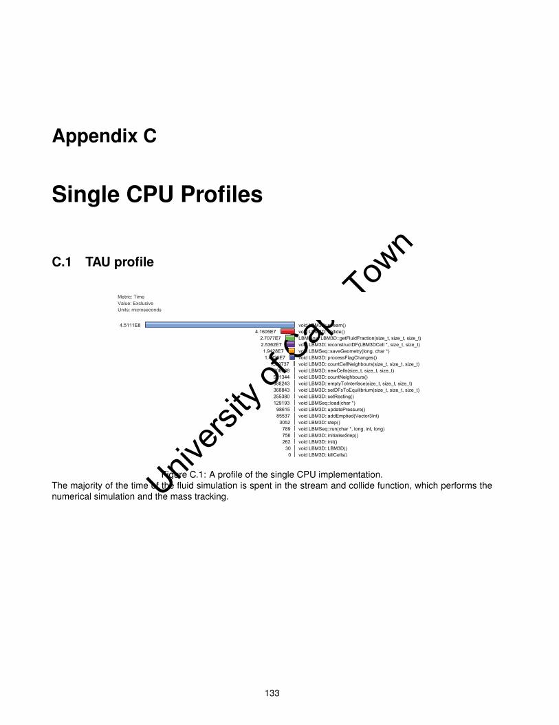
Univers

ity of

Cap

e Tow

n

Appendix C

Single CPU Profiles

C.1 TAU profile

Figure C.1: A profile of the single CPU implementation.The majority of the time of the fluid simulation is spent in the stream and collide function, which performs thenumerical simulation and the mass tracking.

133

Univers

ity of

Cap

e Tow

n

APPENDIX C. SINGLE CPU PROFILES 134

C.2 Operation Counts

Memory Acceses sqrt Floating point Integer operations

Fluid 574 2 401 144

Stream 38 0 0 0

Check neighbour type 19 0 0

Copy appropriate DF 19 0 0

Collide 536 2 401 144

Check for sink cells 1 0 0

Zero current pressure and velocity 1 0 0

Check for override velocity 1 0 0

Calculate current pressure 19 0 19

Calculate current velocity 133 57 57

Current velocity / Pressure 1 0

add gravity force 3 0 3

Save velocity and pressure 3 0 3

Check for fill or empty status 2 0 0

Stability correction 335 2 305 43

La"ce Vector dot current velocity 57 57 0

Calculate Equilibrium-DF 57 61 3

Stress Tensor 216 180 36

Calculate Smagorinsky constant 4 2 4 2

Calculate relaxa#on parameter 1 3 2

Relax DFs to equilibrium 38 38 19

Interface 817 0 538 232

Fetch neighbour types 2 0 0

Calculate Cell Normal 15 0 3 3

Calcula#on 3 3 3

Get Fluid Frac#on (6) 12 0 0

Stream 243 0 127 82

Check neighbour type 19 0 0

Copy appropiate DF 19 0 0

Normal Dot velocity vector 7 3 0

Neighbour type (quan#ty): 0 0

Fluid (5) 15 0 0 10

Mass exchange 3 0 2

Interface(8) 68 0 24 32

Get des#na#on neighbour types 2 0 0

Calculate average mass 2 2 2

Mass exchange 4.5 1 2

Empty (5) 115 0 100 40

Reconstruct DF 23 20 8

Collide 542 0 405 144

as above 536 401 144

correc#on for filled or empty check 6 4 0

Table C.1: The operations used during the stream and collide steps of the LBM for the still pond test case.Totals for the respective cell types are shown with a single line above and a double line below, while sub-totals have a single line below and sub-sub-totals have a single dashed line below. The still pond test case isconsidered, as the fluid division can be predicted.

Univers

ity of

Cap

e Tow

n

Appendix D

Extended Tests and Results

D.1 Latency and bandwidth values for CRUNCH and CHPC

SKaMPI [Reussner, 2002]is a generic benchmarking tool for any MPI implementation. It has a number ofdefault tests for MPI 1 and MPI 2 function sets, but is easily extended to perform specific tests or tests whichhave been left out of the suite. The simple test, Pingpong_Send_Recv, is all that is required to come up withthe estimates we need. First SKaMPI finds the node with the highest latency with the root node, this node isused to perform the measurements. The Pingpong_Send_Recv test records sum of the time taken for the rootnode to send a buffer of defined size to the max latency node and for that node to send a buffer of the samesize back. Recording this time for a number of different buffer sizes yields the graph shown in Figure D.1.A linear regression analysis is used to determine Tstart−up and Tdata for various messages sizes as differentprotocols are used at different times. For above 64kb, CRUNCH has a start-up time of 1614µs and a bandwidthof 8.714µskb−1 at a R2 value of 1, while for below 64kb, the start-up time is 520.8µs and bandwidth 14.05µskb−1

at aR2 value of 0.987. For the CHPC, in region of 0-256kb, we have a start-up time of 87.06µs and bandwidth of2.469µskb−1 at a R2 value of 0.987, while in the region 256kb-1536kb a start-up time of 324.0µs and bandwidthof 1.588µskb−1 at a R2 value of 0.980.

135

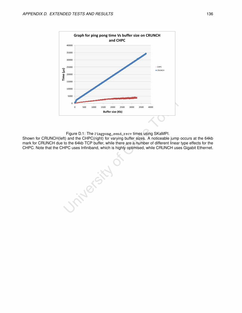
Univers

ity of

Cap

e Tow

n

APPENDIX D. EXTENDED TESTS AND RESULTS 136

0

5000

10000

15000

20000

25000

30000

35000

40000

0 500 1000 1500 2000 2500 3000 3500 4000

Tim

e (

µs)

Buffer size (Kb)

Graph for ping pong time Vs buffer size on CRUNCH and CHPC

CHPC

CRUNCH

Figure D.1: The Pingpong_send_recv times using SKaMPI.Shown for CRUNCH(left) and the CHPC(right) for varying buffer sizes. A noticeable jump occurs at the 64kbmark for CRUNCH due to the 64kb TCP buffer, while there are a number of different linear type effects for theCHPC. Note that the CHPC uses Infiniband, which is highly optimised, while CRUNCH uses Gigabit Ethernet.

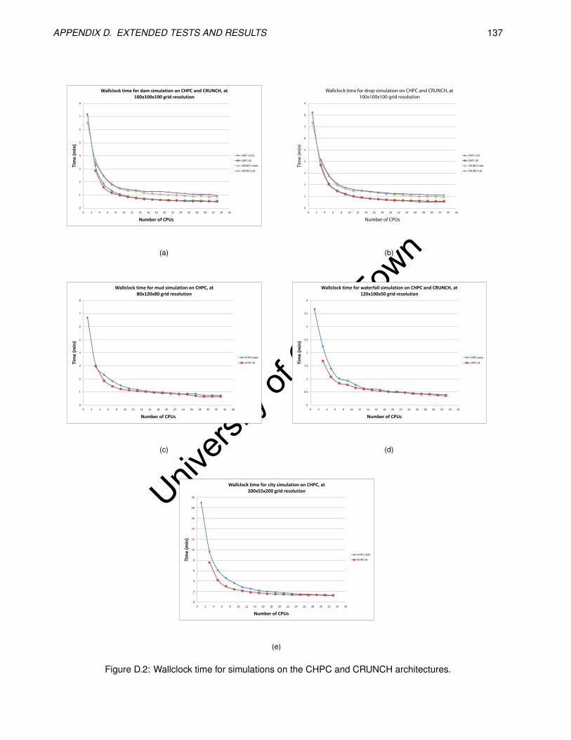
Univers

ity of

Cap

e Tow

n


0

1

2

3

4

5

6

7

8

0 2 4 6 8 10 12 14 16 18 20 22 24 26 28 30 32 34 36

Tim

e (

min

)

Number of CPUs

Wallclock time for dam simulation on CHPC and CRUNCH, at 100x100x100 grid resolution

CHPC-static

CHPC-LB

CRUNCH-static

CRUNCH-LB

(a)

0

1

2

3

4

5

6

7

8

9

0 2 4 6 8 10 12 14 16 18 20 22 24 26 28 30 32 34 36

Tim

e (m

in)

Number of CPUs

Wallclock time for drop simulation on CHPC and CRUNCH, at 100x100x100 grid resolution

CHPC-stat

CHPC-LB

CRUNCH-stat

CRUNCH-LB

(b)

0

1

2

3

4

5

6

7

8

0 2 4 6 8 10 12 14 16 18 20 22 24 26 28 30 32 34 36

Tim

e (

min

)

Number of CPUs

Wallclock time for mud simulation on CHPC, at 80x120x80 grid resolution

CHPC-static

CHPC-LB

(c)

0

0.5

1

1.5

2

2.5

3

3.5

4

0 2 4 6 8 10 12 14 16 18 20 22 24 26 28 30 32 34 36

Tim

e (

min

)

Number of CPUs

Wallclock time for waterfall simulation on CHPC and CRUNCH, at 120x100x50 grid resolution

CHPC-static

CHPC-LB

(d)

0

2

4

6

8

10

12

14

16

18

20

0 2 4 6 8 10 12 14 16 18 20 22 24 26 28 30 32 34 36

Tim

e (

min

)

Number of CPUs

Wallclock time for city simulation on CHPC, at 200x55x200 grid resolution

CHPC-static

CHPC-LB

(e)

Figure D.2: Wallclock time for simulations on the CHPC and CRUNCH architectures.

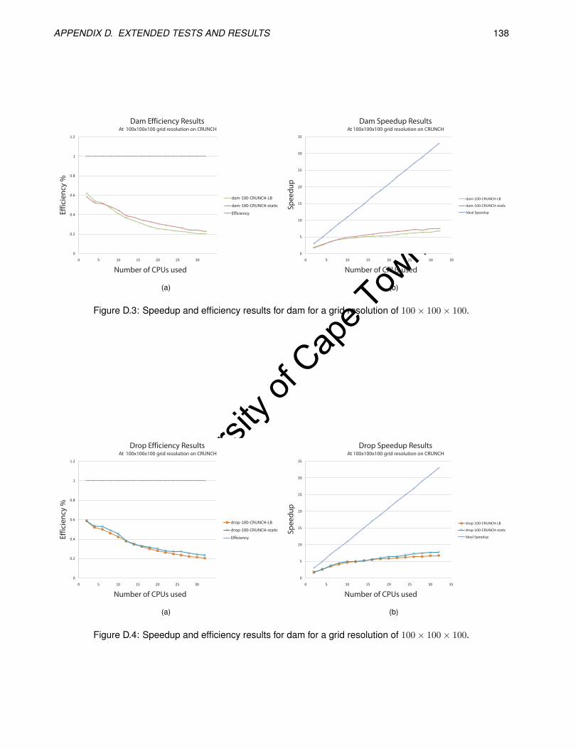
Univers

ity of

Cap

e Tow

n


0

0.2

0.4

0.6

0.8

1

1.2

0 5 10 15 20 25 30

Eff

icie

ncy

%

Number of CPUs used

Dam Efficiency Results At 100x100x100 grid resolution on CRUNCH

dam-100-CRUNCH-LB

dam-100-CRUNCH-sta c

Efficiency

(a)

0

5

10

15

20

25

30

35

0 5 10 15 20 25 30 35

Sp

ee

du

p

Number of CPUs used

Dam Speedup ResultsAt 100x100x100 grid resolution on CRUNCH

dam-100-CRUNCH-LB

dam-100-CRUNCH-sta c

Ideal Speedup

(b)

Figure D.3: Speedup and efficiency results for dam for a grid resolution of 100× 100× 100.

0

0.2

0.4

0.6

0.8

1

1.2

0 5 10 15 20 25 30

Eff

icie

ncy

%

Number of CPUs used

Drop Efficiency ResultsAt 100x100x100 grid resolution on CRUNCH

drop-100-CRUNCH-LB

drop-100-CRUNCH-sta c

Efficiency

(a)

0

5

10

15

20

25

30

35

0 5 10 15 20 25 30 35

Sp

ee

du

p

Number of CPUs used

Drop Speedup ResultsAt 100x100x100 grid resolution on CRUNCH

drop-100-CRUNCH-LB

drop-100-CRUNCH-sta c

Ideal Speedup

(b)

Figure D.4: Speedup and efficiency results for dam for a grid resolution of 100× 100× 100.

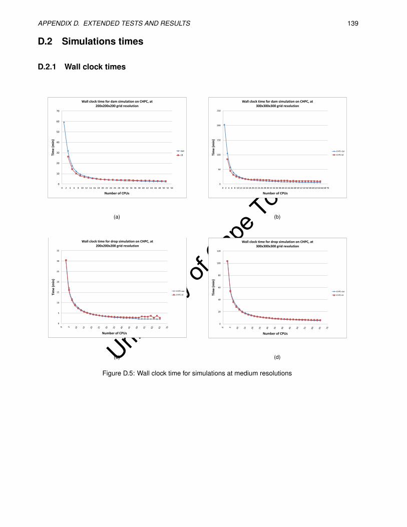
Univers

ity of

Cap

e Tow

n


D.2 Simulations times

D.2.1 Wall clock times

0

10

20

30

40

50

60

70

0 2 4 6 8 10 12 14 16 18 20 22 24 26 28 30 32 34 36 38 40 42 44 46 48 50 52 54

Tim

e (

min

)

Number of CPUs

Wall clock time for dam simulation on CHPC, at 200x200x200 grid resolution

stat

LB

(a)

0

50

100

150

200

250

0 2 4 6 8 10 12 14 16 18 20 22 24 26 28 30 32 34 36 38 40 42 44 46 48 50 52 54 56 58 60 62 64 66 68 70

Tim

e (

min

)

Number of CPUs


CHPC-stat

CHPC-LB

(b)

0

5

10

15

20

25

30

35

Tim

e (

min

)

Number of CPUs

Wall clock time for drop simulation on CHPC, at 200x200x200 grid resolution

CHPC-stat

CHPC-LB

(c)

0

20

40

60

80

100

120

Tim

e (

min

)

Number of CPUs


CHPC-stat

CHPC-LB

(d)

Figure D.5: Wall clock time for simulations at medium resolutions

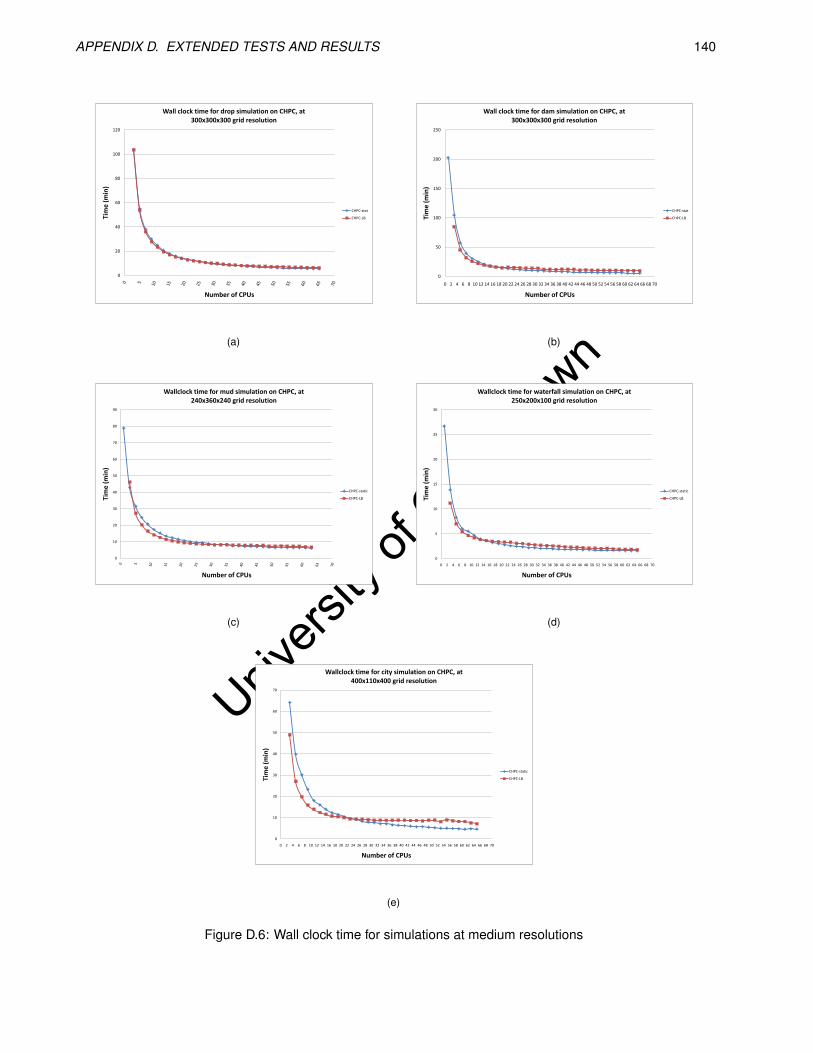
Univers

ity of

Cap

e Tow

n


0

20

40

60

80

100

120

Tim

e (

min

)

Number of CPUs


CHPC-stat

CHPC-LB

(a)

0

50

100

150

200

250

0 2 4 6 8 10 12 14 16 18 20 22 24 26 28 30 32 34 36 38 40 42 44 46 48 50 52 54 56 58 60 62 64 66 68 70

Tim

e (

min

)

Number of CPUs


CHPC-stat

CHPC-LB

(b)

0

10

20

30

40

50

60

70

80

90

Tim

e (

min

)

Number of CPUs


CHPC-static

CHPC-LB

(c)

0

5

10

15

20

25

30

0 2 4 6 8 10 12 14 16 18 20 22 24 26 28 30 32 34 36 38 40 42 44 46 48 50 52 54 56 58 60 62 64 66 68 70

Tim

e (

min

)

Number of CPUs

Wallclock time for waterfall simulation on CHPC, at 250x200x100 grid resolution

CHPC-static

CHPC-LB

(d)

0

10

20

30

40

50

60

70

0 2 4 6 8 10 12 14 16 18 20 22 24 26 28 30 32 34 36 38 40 42 44 46 48 50 52 54 56 58 60 62 64 66 68 70

Tim

e (

min

)

Number of CPUs

Wallclock time for city simulation on CHPC, at 400x110x400 grid resolution

CHPC-static

CHPC-LB

(e)

Figure D.6: Wall clock time for simulations at medium resolutions

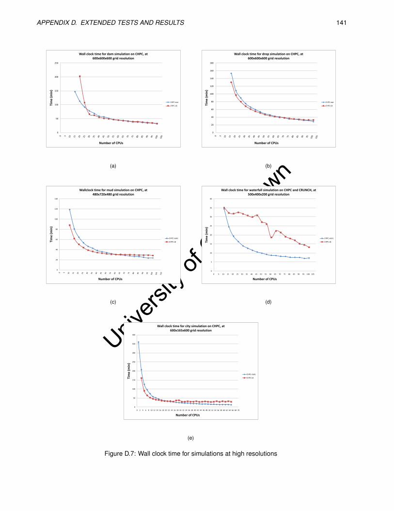
Univers

ity of

Cap

e Tow

n


0

50

100

150

200

250

Tim

e (

min

)

Number of CPUs


CHPC-stat

CHPC-LB

(a)

0

20

40

60

80

100

120

140

160

180

Tim

e (

min

)

Number of CPUs


CHPC-stat

CHPC-LB

(b)

0

20

40

60

80

100

120

140

Tim

e (

min

)

Number of CPUs


CHPC-static

CHPC-LB

(c)

0

5

10

15

20

25

30

35

40

0 5 10 15 20 25 30 35 40 45 50 55 60 65 70 75 80 85 90 95 100 105

Tim

e (

min

)

Number of CPUs

Wall clock time for waterfall simulation on CHPC and CRUNCH, at 500x400x200 grid resolution

CHPC-static

CHPC-LB

(d)

0

50

100

150

200

250

300

350

400

0 2 4 6 8 10 12 14 16 18 20 22 24 26 28 30 32 34 36 38 40 42 44 46 48 50 52 54 56 58 60 62 64 66 68 70

Tim

e (

min

)

Number of CPUs

Wall clock time for city simulation on CHPC, at 600x165x600 grid resolution

CHPC-static

CHPC-LB

(e)

Figure D.7: Wall clock time for simulations at high resolutions

Univers

ity of

Cap

e Tow

n

Bibliography

G. Amati, S. Succi, and R. Piva. Massively Parallel Lattice-Boltzmann Simulation of Turbulent Channel Flow.International Journal of Modern Physics C, 8:869–877, 1997. doi: 10.1142/S0129183197000746.

G.M. Amdahl. Validity of the single processor approach to achieving large scale computing capabilities. InAFIPS Conference Proceedings, volume 30, pages 483–485, 1967.

Yukiya Aoyama and Jun Nakano. RS/6000 SP: Practical MPI Programming. IBM, Austin, Texas, 1999.

D. H. Bailey, E. Barszcz, J. T. Barton, D. S. Browning, R. L. Carter, L. Dagum, R. A. Fatoohi, P. O. Fred-erickson, T. A. Lasinski, R. S. Schreiber, H. D. Simon, V. Venkatakrishnan, and S. K. Weeratunga. Thenas parallel benchmarks—summary and preliminary results. In Supercomputing ’91: Proceedings of the1991 ACM/IEEE conference on Supercomputing, pages 158–165, New York, NY, USA, 1991. ACM. ISBN0-89791-459-7. doi: http://doi.acm.org/10.1145/125826.125925.

Adam W. Bargteil, Tolga G. Goktekin, James F. O’Brien, and John A. Strain. A semi-lagrangian contouringmethod for fluid simulation. ACM Transactions on Graphics, 25(1), 2006.

GK Batchelor. An Introduction to Fluid Dynamics. Cambridge University Press, 2000.

Glen L. Beane. The effects of microprocessor architecture on speedup in distrbuted memory supercomputers.Master’s thesis, The Graduate School The University of Maine, 2004.

M.J. Berger and S.H. Bokhari. A partitioning strategy for nonuniform problems on multiprocessors. IEEETransactions on Computers, 36(5):570–580, 1987. ISSN 0018-9340. doi: http://doi.ieeecomputersociety.

org/10.1109/TC.1987.1676942.

P. L. Bhatnagar, E. P. Gross, and M. Krook. A model for collision processes in gases. i. small amplitudeprocesses in charged and neutral one-component systems. Phys. Rev., 94(3):511–525, May 1954. doi:10.1103/PhysRev.94.511.

Robert Bridson, Ronald Fedkiw, and Matthias Müller-Fischer. Fluid simulation: Siggraph 2006 course notes.In SIGGRAPH ’06: ACM SIGGRAPH 2006 Courses, pages 1–87, New York, NY, USA, 2006. ACM Press.ISBN 1-59593-364-6. doi: http://doi.acm.org/10.1145/1185657.1185730.

Deborah Carlson. Wave displacement effects for surf’s up. In SIGGRAPH ’07: ACM SIGGRAPH 2007sketches, page 91, New York, NY, USA, 2007. ACM. doi: http://doi.acm.org/10.1145/1278780.1278890.

Mark Carlson, Peter J. Mucha, III R. Brooks Van Horn, and Greg Turk. Melting and flowing. In SCA ’02:Proceedings of the 2002 ACM SIGGRAPH/Eurographics symposium on Computer animation, pages 167–174, New York, NY, USA, 2002. ACM Press. ISBN 1-58113-573-4. doi: http://doi.acm.org/10.1145/545261.

545289.

142

Univers

ity of

Cap

e Tow

n

BIBLIOGRAPHY 143

Mark Carlson, Peter J. Mucha, and Greg Turk. Rigid fluid: animating the interplay between rigid bodies andfluid. ACM Trans. Graph., 23(3):377–384, 2004. ISSN 0730-0301. doi: http://doi.acm.org/10.1145/1015706.

1015733.

M.T. Carlson. RIGID, MELTING, AND FLOWING FLUID. PhD thesis, Georgia Institute of Technology, 2004.

Jim X. Chen and Niels da Vitoria Lobo. Toward interactive-rate simulation of fluids with moving obstaclesusing navier-stokes equations. Graph. Models Image Process., 57(2):107–116, 1995. ISSN 1077-3169. doi:http://dx.doi.org/10.1006/gmip.1995.1012.

S. Chen and G. D. Doolen. Lattice Boltzmann Method for Fluid Flows. Annual Review of Fluid Mechanics, 30:329–364, 1998. doi: 10.1146/annurev.uid.30.1.329.

Nuttapong Chentanez, Bryan E. Feldman, François Labelle, James F. O’Brien, and Jonathan R. Shewchuk.Liquid simulation on lattice-based tetrahedral meshes. In SCA ’07: Proceedings of the 2007 ACMSIGGRAPH/Eurographics symposium on Computer animation, pages 219–228, Aire-la-Ville, Switzerland,Switzerland, 2007. Eurographics Association. ISBN 978-1-59593-624-4.

Holger Dachsel, Michael Hofmann, and Gudula Raunger. Library support for parallel sorting in scientific com-putations. In Euro-Par 2007 Parallel Processing, volume 4641 of Lecture Notes in Computer Science, pages695–704. Springer Berlin Heidelberg, 2007. ISBN 978-3-540-74465-8. doi: 10.1007/978-3-540-74466-5_73.URL http://www.springerlink.com/content/avqn88571rt4t4qp/.

P.G. de Gennes, F. Brochard-Wyart, and D. Quéré. Capillarity and Wetting Phenomena: Drops, Bubbles,Pearls, Waves. Springer, 2004.

J.-C. Desplat, I. Pagonabarraga, and P. Bladon. LUDWIG: A parallel Lattice-Boltzmann code for complex fluids.Computer Physics Communications, 134:273–290, March 2001. doi: 10.1016/S0010-4655(00)00205-8.

Dominique d’Humières, Irina Ginzburg, Manfred Krafczyk, Pierre Lallemand, and Li-Shi Luo. Multiple-relaxation-time lattice Boltzmann models in three dimensions. Phil. Trans. R. Soc. A, 360:437–451, 2002.

Jack Dongarra, Ian Foster, Geoffrey Fox, William Gropp, Ken Kennedy, Linda Torczon, and Andy White, editors.Sourcebook of parallel computing. Morgan Kaufmann Publishers Inc., San Francisco, CA, USA, 2003. ISBN1-55860-871-0.

Douglas Enright, Stephen Marschner, and Ronald Fedkiw. Animation and rendering of complex water sur-faces. In SIGGRAPH ’02: Proceedings of the 29th annual conference on Computer graphics and inter-active techniques, pages 736–744, New York, NY, USA, 2002. ACM Press. ISBN 1-58113-521-1. doi:http://doi.acm.org/10.1145/566570.566645.

Z. Fan, F. Qiu, A. Kaufman, and S. Yoakum-Stover. GPU cluster for high performance computing. In Proceed-ings of the 2004 ACM/IEEE conference on Supercomputing, page 47. IEEE Computer Society Washington,DC, USA, 2004.

Raanan Fattal and Dani Lischinski. Target-driven smoke animation. In SIGGRAPH ’04: ACM SIGGRAPH 2004Papers, pages 441–448, New York, NY, USA, 2004. ACM. doi: http://doi.acm.org/10.1145/1186562.1015743.

Ronald Fedkiw, Jos Stam, and Henrik Wann Jensen. Visual simulation of smoke. In SIGGRAPH ’01: Proceed-ings of the 28th annual conference on Computer graphics and interactive techniques, pages 15–22, NewYork, NY, USA, 2001. ACM. ISBN 1-58113-374-X. doi: http://doi.acm.org/10.1145/383259.383260.

Univers

ity of

Cap

e Tow

n

BIBLIOGRAPHY 144

Markus Feilner. OpenVPN: Building and Integrating Virtual Private Networks. Springer-Verlag, New York,1990.

Bryan E. Feldman, James F. O’Brien, and Bryan M. Klingner. Animating gases with hybrid meshes. ACMTrans. Graph., 24(3):904–909, 2005a. ISSN 0730-0301. doi: http://doi.acm.org/10.1145/1073204.1073281.

Bryan E. Feldman, James F. O’Brien, Bryan M. Klingner, and Tolga G. Goktekin. Fluids in deforming meshes.In SCA ’05: Proceedings of the 2005 ACM SIGGRAPH/Eurographics symposium on Computer animation,pages 255–259, New York, NY, USA, 2005b. ACM. ISBN 1-7695-2270-X. doi: http://doi.acm.org/10.1145/

1073368.1073405.

M.J. Flynn. Some computer organizations and their effectiveness. IEEE Transactions on Computers, 21(9):948–960, 1972.

J.D. Foley. Computer Graphics: Principles and Practice. Addison-Wesley Professional, 1995.

Nick Foster and Ronald Fedkiw. Practical animation of liquids. In SIGGRAPH ’01: Proceedings of the 28thannual conference on Computer graphics and interactive techniques, pages 23–30, New York, NY, USA,2001. ACM Press. ISBN 1-58113-374-X. doi: http://doi.acm.org/10.1145/383259.383261.

Nick Foster and Dimitri Metaxas. Realistic animation of liquids. Graph. Models Image Process., 58(5):471–483,1996. ISSN 1077-3169. doi: http://dx.doi.org/10.1006/gmip.1996.0039.

Nick Foster and Dimitris Metaxas. Controlling fluid animation. In CGI ’97: Proceedings of the 1997 Conferenceon Computer Graphics International, page 178, Washington, DC, USA, 1997. IEEE Computer Society. ISBN0-8186-7825-9.

Alain Fournier and William T. Reeves. A simple model of ocean waves. In SIGGRAPH ’86: Proceedings ofthe 13th annual conference on Computer graphics and interactive techniques, pages 75–84, New York, NY,USA, 1986. ACM. ISBN 0-89791-196-2. doi: http://doi.acm.org/10.1145/15922.15894.

U. Frisch, B. Hasslacher, and Y. Pomeau. Lattice-gas automata for the Navier-Stokes equation. PhysicalReview Letters, 56:1505–1508, April 1986.

Uriel Frisch, Dominique dHumi‘eres, Brosl Hasslacher, Pierre Lallemand, Yves Pomeau, and Jean-PierreRivert. Lattice gas hydrodynamics in two and three dimensions. Complex Systems, 1:649–707, 1987.

Richard M. Fujimoto. Parallel simulation: parallel and distributed simulation systems. In WSC ’01: Proceedingsof the 33nd conference on Winter simulation, pages 147–157, Washington, DC, USA, 2001. IEEE ComputerSociety. ISBN 0-7803-7309-X.

Edgar Gabriel, Graham E. Fagg, George Bosilca, Thara Angskun, Jack J. Dongarra, Jeffrey M. Squyres,Vishal Sahay, Prabhanjan Kambadur, Brian Barrett, Andrew Lumsdaine, Ralph H. Castain, David J. Daniel,Richard L. Graham, and Timothy S. Woodall. Open MPI: Goals, concept, and design of a next generation MPIimplementation. In Proceedings, 11th European PVM/MPI Users’ Group Meeting, pages 97–104, Budapest,Hungary, September 2004.

S. Geller, M. Krafczyk, J. Tölke, S. Turek, and J. Hron. Benchmark computations based on lattice-Boltzmann,finite element and finite volume methods for laminar flows. Computers and Fluids, 35(8-9):888–897, 2006.

W. Gropp, E. Lusk, and A. Skjellum. Using MPI: Portable Parallel Programming with the Message PassingInterface. MIT Press, 1999.

Univers

ity of

Cap

e Tow

n

BIBLIOGRAPHY 145

Eran Guendelman, Andrew Selle, Frank Losasso, and Ronald Fedkiw. Coupling water and smoke to thindeformable and rigid shells. ACM Trans. Graph., 24(3):973–981, 2005. ISSN 0730-0301. doi: http://doi.

acm.org/10.1145/1073204.1073299.

J. Hardy, O. de Pazzis, and Y. Pomeau. Molecular dynamics of a classical lattice gas: Transport propertiesand time correlation functions. Phys. Rev. A, 13:1949–1961, May 1976. doi: 10.1103/PhysRevA.13.1949.

Francis H. Harlow and J. Eddie Welch. Numerical calculation of time-dependent viscous incompressible flowof fluid with free surface. Physics of Fluids, 8(12):2182–2189, 1965a. doi: http://scitation.aip.org/jhtml/

doi.jsp.

Francis H. Harlow and J. Eddie Welch. Numerical calculation of time-dependent viscous incompressible flowof fluid with free surface. Physics of Fluids, 8(12):2182–2189, 1965b. doi: 10.1063/1.1761178. URL http:

//link.aip.org/link/?PFL/8/2182/1.

Xiaoyi He and Li-Shi Luo. A priori derivation of the lattice boltzmann equation. Phys. Rev. E, 55(6):R6333–R6336, Jun 1997. doi: 10.1103/PhysRevE.55.R6333.

N.J. Higham. Accuracy and stability of numerical algorithms. Siam, 2002.

F. J. Higuera and J. Jiménez. Boltzmann approach to lattice gas simulations. Europhysics Letters, 9:663–+,August 1989.

F. J. Higuera, S. Succi, and R. Benzi. Lattice gas dynamics with enhanced collisions. Europhysics Letters, 9:345–+, June 1989.

S. Hou, J. Sterling, S. Chen, and G. D. Doolen. A Lattice Boltzmann Subgrid Model for High Reynolds NumberFlows. Contributions to Mineralogy and Petrology, pages 1004–+, January 1994.

Lee Howes and David Thomas. Real time simulation and rendering of 3d fluids. In Hubert Nguyen, editor,GPU Gems 3. Addison Wesley, 2007.

Geoffrey Irving, Eran Guendelman, Frank Losasso, and Ronald Fedkiw. Efficient simulation of large bodies ofwater by coupling two and three dimensional techniques. In SIGGRAPH ’06: ACM SIGGRAPH 2006 Papers,pages 805–811, New York, NY, USA, 2006. ACM Press. ISBN 1-59593-364-6. doi: http://doi.acm.org/10.

1145/1179352.1141959.

D. Kandhai, A. Koponen, A. G. Hoekstra, M. Kataja, J. Timonen, and P. M. A. Sloot. Lattice-Boltzmannhydrodynamics on parallel systems. Computer Physics Communications, 111:14–26, June 1998. doi:10.1016/S0010-4655(98)00025-3.

George Karypis and Vipin Kumar. Multilevel k -way hypergraph partitioning. In Design Automation Conference,pages 343–348, 1999. URL citeseer.ist.psu.edu/article/karypis98multilevel.html.

Michael Kass and Gavin Miller. Rapid, stable fluid dynamics for computer graphics. In SIGGRAPH ’90: Pro-ceedings of the 17th annual conference on Computer graphics and interactive techniques, pages 49–57,New York, NY, USA, 1990. ACM Press. ISBN 0-201-50933-4. doi: http://doi.acm.org/10.1145/97879.97884.

Richard Keiser, Bart Adams, Dominique Gasser, Paolo Bazzi1 Philip Dutrï¿12 , and Markus Gross. A unified

lagrangian approach to solid-fluid animation. Point-Based Graphics, 20(21):125–148, 2005.

Richard Keiser, Bart Adams, Leonidas J. Guibas, Philip Dutri, and Mark Pauly. Multiresolution particle-basedfluids. Technical report, ETH CS, 2006.

Univers

ity of

Cap

e Tow

n

BIBLIOGRAPHY 146

Bryan M. Klingner, Bryan E. Feldman, Nuttapong Chentanez, and James F. O’Brien. Fluid animation withdynamic meshes. In Proceedings of ACM SIGGRAPH 2006, pages 820–825, August 2006.

C. Körner and R. F. Singer. Processing of metal foams| -| challenges and opportunities. Advanced EngineeringMaterials, 2(4):159–165, 2000. ISSN 1527-2648.

C. Körner, M. Thies, and R.F. Singer. Modeling of metal foaming with lattice boltzmann automata. Advancedengineering materials(Print), 4(10), 2002.

Carolin Körner, Thomas Pohl, , Nils Thürey, and Thomas Zeiser. Parallel Lattice Boltzmann Methods for CFDApplications, volume 51. Springer Berlin Heidelberg, 2006.

Géraud Krawezik. Performance comparison of mpi and three openmp programming styles on shared memorymultiprocessors. In SPAA ’03: Proceedings of the fifteenth annual ACM symposium on Parallel algorithmsand architectures, pages 118–127, New York, NY, USA, 2003. ACM. ISBN 1-58113-661-7. doi: http:

//doi.acm.org/10.1145/777412.777433.

W. Li, X. Wei, and A. Kaufman. Implementing lattice Boltzmann computation on graphics hardware. The VisualComputer, 19(7):444–456, 2003.

A. Lindenmayer. Adding Continuous Components to L-Systems. Lecture Notes In Computer Science; Vol. 15,pages 53–68, 1974.

Mats Lindh. Marching cubes implementation, March 2003. http://www.ia.hiof.no/~borres/cgraph/

explain/marching/p-march.html.

William E. Lorensen and Harvey E. Cline. Marching cubes: A high resolution 3d surface construction algorithm.SIGGRAPH Comput. Graph., 21(4):163–169, 1987. ISSN 0097-8930. doi: http://doi.acm.org/10.1145/

37402.37422.

F. Losasso, G. Irving, E. Guendelman, and R. Fedkiw. Melting and Burning Solids into Liquids and Gases.IEEE TRANSACTIONS ON VISUALIZATION AND COMPUTER GRAPHICS, pages 343–352, 2006a.

Frank Losasso, Frédéric Gibou, and Ron Fedkiw. Simulating water and smoke with an octree data structure.In SIGGRAPH ’04: ACM SIGGRAPH 2004 Papers, pages 457–462, New York, NY, USA, 2004. ACM. doi:http://doi.acm.org/10.1145/1186562.1015745.

Frank Losasso, Tamar Shinar, Andrew Selle, and Ronald Fedkiw. Multiple interacting liquids. ACM Trans.Graph., 25(3):812–819, 2006b. ISSN 0730-0301. doi: http://doi.acm.org/10.1145/1141911.1141960.

Frank Losasso, Jerry Talton, Nipun Kwatra, and Ronald Fedkiw. Two-way coupled sph and particle level setfluid simulation. IEEE Transactions on Visualization and Computer Graphics, 14(4):797–804, 2008. ISSN1077-2626. doi: http://dx.doi.org/10.1109/TVCG.2008.37.

Hai Mao and Yee-Hong Yang. Particle-based immiscible fluid-fluid collision. In GI ’06: Proceedings of the2006 conference on Graphics interface, pages 49–55, Toronto, Ont., Canada, Canada, 2006. CanadianInformation Processing Society. ISBN 1-56881-308-2.

Guy R. McNamara and Gianluigi Zanetti. Use of the boltzmann equation to simulate lattice-gas automata.Phys. Rev. Lett., 61(20):2332–2335, Nov 1988. doi: 10.1103/PhysRevLett.61.2332.

Gavin Miller and Andrew Pearce. Globular dynamics: A connected particle system for animating viscous fluids.Computers and Graphics, 13(3):305–309, 1989. URL citeseer.ist.psu.edu/miller89globular.html.

Univers

ity of

Cap

e Tow

n

BIBLIOGRAPHY 147

B. Mohr, D. Brown, and A. Malony. TAU: A Portable Parallel Program Analysis Environment for pC++. LEC-TURE NOTES IN COMPUTER SCIENCE, pages 29–29, 1994.

C. Montani, R. Scateni, and R. Scopigno. Discretized marching cubes. In Proceedings of the conference onVisualization’94, pages 281–287. IEEE Computer Society Press Los Alamitos, CA, USA, 1994.

Dirk Muders. Three-Dimensional Parallel Lattice Boltzmann Hydrodynamic Simulations of Turbulent Flows inInterstellar Dark Clouds. PhD thesis, Rheinischen Friedrich-Wilhelms-Universitat, 1995.

Matthias Müller, David Charypar, and Markus Gross. Particle-based fluid simulation for interactive applications.In SCA ’03: Proceedings of the 2003 ACM SIGGRAPH/Eurographics symposium on Computer animation,pages 154–159, Aire-la-Ville, Switzerland, Switzerland, 2003. Eurographics Association. ISBN 1-58113-659-5.

Matthias Müller, Barbara Solenthaler, Richard Keiser, and Markus Gross. Particle-based fluid-fluid interaction.In SCA ’05: Proceedings of the 2005 ACM SIGGRAPH/Eurographics symposium on Computer animation,pages 237–244, New York, NY, USA, 2005. ACM Press. ISBN 1-7695-2270-X. doi: http://doi.acm.org/10.

1145/1073368.1073402.

Duc Quang Nguyen, Ronald Fedkiw, and Henrik Wann Jensen. Physically based modeling and animation offire. In SIGGRAPH ’02: Proceedings of the 29th annual conference on Computer graphics and interactivetechniques, pages 721–728, New York, NY, USA, 2002. ACM Press. ISBN 1-58113-521-1. doi: http:

//doi.acm.org/10.1145/566570.566643.

P. Ning and J. Bloomenthal. An evaluation of implicit surface tilers. IEEE Computer Graphics and Applications,13(6):33–41, 1993.

Karonis N.T. Mpich-g2: A grid-enabled implementation of the message passing interface. Journal of Paralleland Distributed Computing, 63:551–563(13), May 2003. URL http://www.ingentaconnect.com/content/

els/07437315/2003/00000063/00000005/art00002.

J. Paul Peszko. Water, water, everywhere..., 2006. www.vfxworld.com.

Nils Thürey Thomas Pohl and Ulrich Rüde. Hybrid Parallelization Techniques for Lattice Boltzmann FreeSurface Flows. International Conference on Parallel Computational Fluid Dynamics, May 2007.

TJ Poinsot and SK Lele. Boundary conditions for direct simulations of compressible viscous flows. Journal ofcomputational physics(Print), 101(1):104–129, 1992.

Simon Premoze, Tolga Tasdizen, James Bigler, Aaron Lefohn, and Ross Whitaker. Particle-based simulationof fluids. Eurographics 2003, 22(3), 2003.

W.H. Press, B. FLANNERY, S.A. TEUKOLSKY, W.T. VETTERLING, et al. Numerical recipes. CambridgeUniversity Press New York, 1986.

Y. H. Qian, D. D’Humières, and P. Lallemand. Lattice BGK models for Navier-Stokes equation. EurophysicsLetters, 17:479–+, February 1992.

RM Ramanathan, P. Contributors, R. Curry, S. Chennupaty, R.L. Cross, S. Kuo, and M.J. Buxton. Extendingthe World’s Most Popular Processor Architecture. Technology intel Magazine, 2006.

R. Reussner. SKaMPI: a comprehensive benchmark for public benchmarking of MPI. Scientific Programming,10(1):55–65, 2002.

Univers

ity of

Cap

e Tow

n

BIBLIOGRAPHY 148

M. Roy, S. Foufou, and F. Truchetet. Mesh Comparison Using Attribute Deviation Metric. International Journalof Image and Graphics, 4(1):127–140, 2004.

Andrew Selle, Nick Rasmussen, and Ronald Fedkiw. A vortex particle method for smoke, water and explosions.ACM Trans. Graph., 24(3):910–914, 2005. ISSN 0730-0301. doi: http://doi.acm.org/10.1145/1073204.

1073282.

Maddu Shankar and S. Sundar. Asymptotic analysis of extrapolation boundary conditions for lbm. Comput.Math. Appl., 57(8):1313–1323, 2009. ISSN 0898-1221. doi: http://dx.doi.org/10.1016/j.camwa.2009.01.018.

Lin Shi and Yizhou Yu. Taming liquids for rapidly changing targets. In SCA ’05: Proceedings of the 2005 ACMSIGGRAPH/Eurographics symposium on Computer animation, pages 229–236, New York, NY, USA, 2005.ACM Press. ISBN 1-7695-2270-X. doi: http://doi.acm.org/10.1145/1073368.1073401.

Samuel Silva, Joaquim Madeira, and Beatriz Sousa Santos. Polymeco " a polygonal mesh comparison tool.In IV ’05: Proceedings of the Ninth International Conference on Information Visualisation, pages 842–847,Washington, DC, USA, 2005. IEEE Computer Society. ISBN 0-7695-2397-8. doi: http://dx.doi.org/10.1109/IV.2005.98.

Jos Stam. Stable fluids. In SIGGRAPH ’99: Proceedings of the 26th annual conference on Computer graphicsand interactive techniques, pages 121–128, New York, NY, USA, 1999. ACM Press/Addison-Wesley Pub-lishing Co. ISBN 0-201-48560-5. doi: http://doi.acm.org/10.1145/311535.311548.

Markus Sturmer, Jan Gotz, Gregor Richter, and U. Rude. Blood flow simulation on the cell broadband engineusing the lattice boltzmann method. Technical report, Technical Report 07-9. Technical report, Departmentof Computer Science 10 System Simulation, 2007.

Sauro Succi. The Lattice Boltzmann Euqation for fluid dynamics and beyond. Oxford University Press, NewYork, 2001.

Mark Sussman. A second order coupled level set and volume-of-fluid method for computing growth andcollapse of vapor bubbles. J. Comput. Phys., 187(1):110–136, 2003. ISSN 0021-9991. doi: http:

//dx.doi.org/10.1016/S0021-9991(03)00087-1.

Nils Thuerey. Free surface flows with lbm, October 2008. http://www.vgtc.org/PDF/slides/2008/visweek/tutorial8_thuerey.pdf.

N. Thurey, C. Korner, and U. Rude. Interactive Free Surface Fluids with the Lattice Boltzmann Method. Techni-cal report, Technical Report 05-4. Technical report, Department of Computer Science 10 System Simulation,2005a.

N. Thurey, C. Korner, and U. Rude. Interactive Free Surface Fluids with the Lattice Boltzmann Method. Techni-cal report, Technical Report 05-4. Technical report, Department of Computer Science 10 System Simulation,2005, 2005b.

N. Thurey, K. Iglberger, and U. Rude. Free surface flows with moving and deforming objects with LBM. InVision, Modeling, and Visualization, 2006.

N. Thürey, R. Keiser, and M. Pauly Ulrich Rüde. Detail-preserving fluid control. In SCA ’06: Proceedingsof the 2006 ACM SIGGRAPH/Eurographics symposium on Computer animation, pages 7–12, Aire-la-Ville,Switzerland, Switzerland, 2006. Eurographics Association. ISBN 3-905673-34-7.

Univers

ity of

Cap

e Tow

n

BIBLIOGRAPHY 149

N. Thürey, T. Pohl, U. Rüde, M. Öchsner, and C. Körner. Optimization and stabilization of LBM free surfaceflow simulations using adaptive parameterization. Computers and Fluids, 35(8-9):934–939, 2006.

Nils Thürey. A single-phase free-surface lattice-boltzmann method. Master’s thesis, FRIEDRICH-ALEXANDER-UNIVERSITÄT ERLANGEN-NÜRNBERG, 2003.

Nils Thurey. Physically based Animation of Free Surface Flows with the Lattice Boltzmann Method. PhD thesis,Technischen Fakultat der Universitat Erlangen-Nurnberg, 2007.

Nils Thürey and Ulrich Rüde. Optimized free surface fluids on adaptive grids with the lattice boltzmann method.In SIGGRAPH ’05: ACM SIGGRAPH 2005 Posters, page 112, New York, NY, USA, 2005. ACM. doi: http://doi.acm.org/10.1145/1186954.1187082.

Nils Thürey and Ulrich Rüde. "stable free surface flows with the lattice boltzmann method on adaptively coars-ened grids". Computing and Visualization in Science, 2008.

Stephan Trojansky, Thomas Ganshorn, and Oliver Pilarski. 300’s liquid battlefield: fluid simulation spartanstyle. In SIGGRAPH ’07: ACM SIGGRAPH 2007 sketches, page 95, New York, NY, USA, 2007. ACM. doi:http://doi.acm.org/10.1145/1278780.1278894.

T. N. Venkatesh, V. R. Sarasamma, Rajalakshmy S., Kirti Chandra Sahu, and Rama Govindarajan. Super-linearspeed-up of a parallel multigrid Navier-Stokes solver on Flosolver. RESEARCH ARTICLES, 88:589–593,2004.

Junye Wang, Xiaoxian Zhang, Anthony G. Bengough, and John W. Crawford. Domain-decomposition methodfor parallel lattice boltzmann simulation of incompressible flow in porous media. Physical Review E (Sta-tistical, Nonlinear, and Soft Matter Physics), 72(1):016706, 2005. doi: 10.1103/PhysRevE.72.016706. URLhttp://link.aps.org/abstract/PRE/v72/e016706.

Xiaoming Wei, Ye Zhao, Zhe Fan, Wei Li, Suzanne Yoakum-Stover, and Arie Kaufman. Blowing in the wind.In SCA ’03: Proceedings of the 2003 ACM SIGGRAPH/Eurographics symposium on Computer animation,pages 75–85, Aire-la-Ville, Switzerland, Switzerland, 2003. Eurographics Association. ISBN 1-58113-659-5.

Xiaoming Wei, Wei Li, Klaus Mueller, and Arie E. Kaufman. The lattice-boltzmann method for simulatinggaseous phenomena. IEEE Transactions on Visualization and Computer Graphics, 10(2):164–176, 2004a.ISSN 1077-2626. doi: http://dx.doi.org/10.1109/TVCG.2004.1260768.

Xiaoming Wei, Wei Li, Klaus Mueller, and Arie E. Kaufman. The lattice-boltzmann method for simulatinggaseous phenomena. IEEE Transactions on Visualization and Computer Graphics, 10(2):164–176, 2004b.ISSN 1077-2626. doi: http://dx.doi.org/10.1109/TVCG.2004.1260768.

Jens Wilke, Thomas Pohl, Markus Kowarschik, and Ulrich Ruede. Cache performance optimizations for parallellattice boltzmann codes. In Euro-Par 2003 Parallel Processing, volume 2790 of Lecture Notes in ComputerScience, pages 441–450. Springer Berlin / Heidelberg, 2003. ISBN 978-3-540-40788-1. doi: 10.1007/

b12024. URL http://www.springerlink.com/content/p7jagg6fjvt4ryec/.

B. Wilkinson and M. Allen. Parallel programming: techniques and applications using networked workstationsand parallel computers. Prentice-Hall, Inc. Upper Saddle River, NJ, USA, 1998.

Dieter A. Wolf-Gladrow. Lattice-Gas Cellular Automata and lattice Boltzmann Models. Springer-Verlag, NewYork, 2000.

Yongning Zhu and Robert Bridson. Animating sand as a fluid. ACM Trans. Graph., 24:965–972, 2005.

RI&DSH7RZQ - COnnecting REpositories · The creation of automated ﬂuid effects for ﬁlm and...

Documents

Transcript of RI&DSH7RZQ - COnnecting REpositories · The creation of automated ﬂuid effects for ﬁlm and...