Riders on the Storm - Kansas City Fed
44
17 Riders on the Storm Òscar Jordà and Alan M. Taylor He stood in reverential awe of himself; he had performed a miraculous feat. The act of finding himself on the face of the waters became a rite, and he felt himself a superior being to the rest of us who knew not this rite and were dependent on him for being shepherded across the heaving and limitless waste, the briny highroad that connects the continents and whereon there are no mile-stones. So, with the sextant he made obeisance to the sun-god, he consulted ancient tomes and tables of magic characters, muttered prayers in a strange tongue that sounded like INDEXERRORPARALLAXREFRAC- TION, made cabalistic signs on paper, added and carried one, and then, on a piece of holy script called the Grail—I mean the Chart—he placed his finger on a certain space conspicuous for its blankness and said, “Here we are.” When we looked at the blank space and asked, “And where is that?” he answered in the cipher-code of the higher priesthood, “31-15-47 north, 133-5-30 west.” And we said “Oh,” and felt mighty small. — Jack London, The Cruise of the Snark I. The Rise and Fall of r* and Monetary Policy Navigation The stabilization of inflation and of the business cycle are core ob- jectives of a central bank. Rightfully, monetary economics has spent a great deal of effort detailing how policymakers should set interest rates as they strive to attain these objectives in a given environment. Yet environments can change, and neither central bankers nor the
Transcript of Riders on the Storm - Kansas City Fed

17
Riders on the Storm
Òscar Jordà and Alan M. Taylor
He stood in reverential awe of himself; he had performed a miraculous feat. The act of finding himself on the face of the waters became a rite, and he felt himself a superior being to the rest of us who knew not this rite and were dependent on him for being shepherded across the heaving and limitless waste, the briny highroad that connects the continents and whereon there are no mile-stones. So, with the sextant he made obeisance to the sun-god, he consulted ancient tomes and tables of magic characters, muttered prayers in a strange tongue that sounded like INDEXERRORPARALLAXREFRAC-TION, made cabalistic signs on paper, added and carried one, and then, on a piece of holy script called the Grail—I mean the Chart—he placed his finger on a certain space conspicuous for its blankness and said, “Here we are.” When we looked at the blank space and asked, “And where is that?” he answered in the cipher-code of the higher priesthood, “31-15-47 north, 133-5-30 west.” And we said “Oh,” and felt mighty small.
— Jack London, The Cruise of the Snark
I. The Rise and Fall of r* and Monetary Policy Navigation
The stabilization of inflation and of the business cycle are core ob-jectives of a central bank. Rightfully, monetary economics has spent a great deal of effort detailing how policymakers should set interest rates as they strive to attain these objectives in a given environment. Yet environments can change, and neither central bankers nor the

18 Òscar Jordà and Alan M. Taylor
economic system exist in isolation from outside influences. In this paper we show that global forces set the course of interest rates over the medium to long run. This happens to a degree perhaps insuffi-ciently appreciated. Navigating policy through the economy’s stormy waters therefore requires a good reading of local currents as much as underlying yet powerful global disturbances.
Specifically, we address basic questions about the workings of mon-etary policy with evidence drawn from the recent history of advanced economies. What are the drivers of monetary policy and how should we measure them? How truly independent of each other are different central banks? Are the drivers domestic or international? What are the implications of this mix of forces for monetary policy?
The key framing in our paper is the distinction between, on the one hand, how central banks steer by tightening and loosening their stance in response to local cyclical macroeconomic conditions; and on the other hand, how wider forces can permeate interest rate set-tings through the drift of the natural real rate of interest, or r*, at both local and global levels.
To sharpen the distinction: looking only to the natural rate for guid-ance could be referred to as “navigating by the stars” (Powell 2018), and would be one extreme approach to policy; conversely, using only local cyclical conditions for pilotage would be akin to navigating by nearby clues like landmarks, at the other extreme. As a shorthand, let us refer to these two polar extremes as celestial navigation and terrestrial navigation, respectively. One might think that in reality policymakers would rely on both guides, and indeed we will argue that, as an empiri-cal description of reality, both have mattered. Our analysis then docu-ments the roles that each has played, their relative importance, and the guide they provide to macroeconomic outcomes.
The backdrop to our discussion is a rising worry among policy-makers about the re-emergence of policy divergence and what it portends. After the global financial crisis, central banks in advanced economies lowered interest rates aggressively and ended up near zero. Policy was tuned to a deep recession context and the common nature

Riders on the Storm 19
of the shock pushed policy stances everywhere into high accommo-dation, albeit constrained by an effective lower bound.
In that milieu, at first glance, policy synchronization appeared to reach an extreme not seen for about 70 years, going back to a similar configuration in the Great Depression of the 1930s. Yet the failure to see autonomy being used—in the sense of divergent interest rate settings—did not, of course, imply that autonomy had disappeared. When, in response to asymmetrical recovery patterns, some but not all central banks began “liftoff,” this triggered dormant anxieties about the negative spillovers and stresses that non-coordinated policy divergence might place upon the system. As the trilemma teaches us, when autonomy is eventually exercised, in a world of capital mobility this must inevitably perturb exchange rate equilibrium. But political rhetoric and economic logic can often part ways, and now talk of currency wars and exchange rate manipulation has once more started to make headlines.
Beyond all the heat, can we shed light? Without firmer empirical evidence, of the kind we present here, it is difficult to know how concerned we should be. And the fact that long-run forces matter, that these forces are beyond policymakers’ control, and also contain a strong global component, means that our argument could support a more benign narrative.
The idea that monetary policymakers are forced to adapt to long-run global trends as much, or even more, than adjusting to short-run local stabilization objectives may seem controversial—economically, as well as politically. In theory, central bank independence insulates societies from short-term politics in favor of long-run welfare gains. Indeed, central banks readily admit to trading off the short term for the long run. Yet few would admit trading off domestic interests for those abroad, even when doing so might be better in the long run. Politics matters here, clearly. But even on economic grounds there is, at least under special conditions, a theoretical basis for looking in-ward, since in complete, frictionless international asset markets with efficient risk sharing, central banks can achieve optimal stabilization outcomes based on domestic considerations alone.1 But of course,

20 Òscar Jordà and Alan M. Taylor
the world is more complicated, and that forces us to consider how and why it matters.
The questions at hand—what drives monetary policy and where do we stand now?—can only be addressed by first solving two prob-lems. First, as a conceptual matter, our point of departure must make the correct definition of terms to properly measure monetary policy stance, since this can be the only basis for sound analysis. Second, as an empirical matter, we must embrace a long-term multicountry perspective to properly judge current policy conditions relative to a sufficiently large sample of historical outcomes.
We take the view that the stance of monetary policy is rigorously described by the deviation of the prevailing policy rate or relevant short-term real interest rate (r ) from the corresponding short-term neutral or Wicksellian natural real rate (r* ). The key challenge here is that the latter is unobservable, yet simply to use the former would produce mismeasurement. If the neutral rate of interest declines fast-er than the central bank cuts nominal rates, financial conditions will be tighter, even if, on the surface, the central bank appears to be loos-ening them. As we aim to cast back over several decades in this paper, our empirical analysis of the causes and consequences of monetary policy divergence first requires plausible estimates of the natural rate in major advanced economies and this is a major task that occupies us in the first part of the paper.
Section II leads off with the empirical core of our analysis. It cen-ters on an empirical, state-space model of the natural rate which builds on the seminal work done by Laubach and Williams (2003), and later taken to international data in Holston, Laubach and Wil-liams (2017). Here the approach is augmented to incorporate ad-ditional information from yields on long-term government bonds. In this setup, all bond yields incorporate the natural real rate plus additional components reflecting term premiums. We can better pin down the common trend in the benchmark natural rate if we utilize more than one maturity, while allowing for the term premiums to vary by period and by country.

Riders on the Storm 21
After describing this augmented model, we then apply it to a post-World War II sample of annual data for four major advanced econo-mies: the United States, Japan, Germany and the United Kingdom. The model produces sensible and plausible estimates of the two key latent state variables, the natural rate of interest and the growth rate of potential output. Beyond these we can use the model to construct many important summary indicators for our analysis.
The model output reveals new, interesting and plausible long-run trends in the natural rate in the advanced economies over the last 60 years with implications for wider debates about the drivers of growth and the phenomenon of secular stagnation. Later in the paper, when we look into macroeconomic adjustment, we let these estimates speak to the mechanics of celestial navigation. We can obtain the measure of monetary policy, or stance (actual short rate minus natural rate), and how far the economy is from its potential, or gap (actual minus potential output). Later in the paper we let these estimates speak to the mechanics of terrestrial navigation.
In Sections III and IV, we take the model estimates and construct the analytic narrative. Here we aim to develop a quantitative inter-pretation of the postwar history of monetary policymaking in the four major advanced economies. We present many findings.
From 1985, and for the last 30 years, we find a common, declin-ing r* in all countries; previously r* had been rising, especially in the 1970s. The finding is not new in itself, but now confirmed even in a model with term premiums. We find that all economies have a strong common global component in their r* measure. They also have a strong common global component in two subcomponents of r*. The first of these is attributable to potential output growth and the second captures other latent factors. Each explains about half the global variation in r*. The term premiums vary much less and have been relatively stable in the last 30 years or so.
We find that all economies have a strong common global compo-nent in their output gap measure gap. They also have a strong com-mon global component in their policy measure stance. Despite the focus of much empirical and theoretical work on the local economy

22 Òscar Jordà and Alan M. Taylor
determinants of stance, we find that most of the variation in short rates is not accounted for by stance at all. Rather, over the long run, variation in the local and world paths of the natural rate is consider-able. We find a cross-country convergence of both gap and stance, which have seen falling dispersion since 1970. But for stance this was not monotonic, as policy dispersion rose to high levels from the late 1970s to the early 1990s. This is intuitive, given the chaotic nature of monetary policy execution from the collapse for Bretton Woods to the start of inflation targeting.
Section V then investigates the predictive value of the model es-timates for key short-run local macroeconomic outcomes and asks whether these accord with conventional wisdom. The dynamics of gap and stance are intuitive and plausible. A positive change in stance predicts a negative change in gap: a tighter policy tends to lead an output slowdown. A positive change in gap predicts a positive change in stance: an output acceleration tends to lead a tighter policy.
Lastly, Section VI investigates the predictive value of the model estimates for a range of medium-run open-economy macroeconomic outcomes and asks whether these also accord with conventional wis-dom. Here, we try to assess whether the inferred measures of the neutral real rate r* from the state-space estimation align with text-book descriptions on the workings of the international adjustment mechanisms. This broad cross-check on whether the model makes sense proves encouraging and we find that, based on the differen-tial between the county r* and the world r*, a higher relative local r* today is associated subsequently, over the medium-term horizon, with higher output relative to potential; higher inflation relative to steady state; a tighter policy stance; a stronger exchange rate; a larger current account deficit; a lower saving rate; a higher investment rate; and stronger growth in real credit creation. All these responses accord well with standard economic logic in an open economy setting with divergent natural real rates and adjustment frictions (Clarida 2019, Obstfeld 2019).
Section VII concludes with the policy implications of our analy-sis. Briefly, in a financially integrated world where capital can move freely across borders with increasing ease, central banks should tack

Riders on the Storm 23
in response to local conditions while at the same time observing the drift of economic currents implied by disturbances in the neutral rate near and far. Ignoring such trends risks provoking internal and ex-ternal imbalances, as well as unwanted dislocation in credit markets, eventually carrying the economy off course.
II. Description of the Model
The Wicksellian natural rate of interest is a yardstick for the stance of monetary policy. Although Wicksell (1936 [1898]) initially de-fined the natural or neutral rate as a short-term interest rate that keeps output at its potential level and prices stable, numerous refine-ments have emerged since Woodford’s (2003) influential textbook and Laubach and Williams’ (2003) estimates, with some divergence emerging between short- and long-run versions of the natural rate in subsequent work by others.
The approach that we take is pragmatic. Cast against a canonical New Keynesian model, our estimate of the natural rate is pinned down by both the IS curve, which spells out the relationship between output gaps and deviations of the real rate from its natural rate, and the Phillips curve, which then relates inflation to past and future expected inflation and the output gap. In the long run, the natural rate ensures that output is at potential and, hence, the growth rate of potential output is a key determinant of the natural rate. Our aug-mented model also views long term bond yields as being determined by the natural rate, inflation expectations, and a term premium.
The essential problem is that the natural rate is not directly observ-able and neither are several of the key variables. Hence our model contains several unobserved latent processes or state variables that have to be estimated via Maximum Likelihood methods through a specification of the corresponding state-space representation and us-ing the Kalman filter.
Our model can be summarized by the following equations, orga-nized by block. We begin with the set of equations which describe the stochastic process for potential output and hence its rate of growth. Let 𝑦t denote 100 times the log of real GDP, and *yt denote 100 times the log of potential real GDP, treated as an unobserved state

24 Òscar Jordà and Alan M. Taylor
variable. The latter has a first difference denoted by gt , also an un-
observed state variable assumed to follow a random walk. Finally, let x
t denote the output gap, with analogous log scaling, defined as the
difference between actual and potential output. The specification of this block of equations is the same as that in Laubach and Williams (2003) and used in subsequent research by many others. Summariz-ing, potential output and its growth rate are determined by the fol-lowing expressions,
yt* ≡ yt −1* + gt , (1)
gt = gt −1 +vtg , (2)
xt ≡ yt − yt*. (3)
We now let rt denote the ex-ante real rate on short-term govern-
ment bills, specifically, rt = it −π t t −1* And let rt* denote the associated
neutral real rate of interest for this asset. We specify the IS curve re-lating the output gap to the lagged output gap and deviations of the real rate from its neutral level, plus an error term, such that
xt = φxt −1 − γ rt −1 − rt −1*( )+vtx , (4)
where 𝜙, 𝛾 > 0. To simplify the model, and for symmetry with respect to subsequent expressions, we restrict 𝜙 = 0.65 but leave 𝛾 otherwise unrestricted.
The neutral rate of interest is assumed to be determined by the sum of two components, a latent trend factor z
t and the growth rate of po-
tential output defined earlier as gt. This specification of the stochastic
process of the neutral rate also borrows from Laubach and Williams (2003), and implies that
zt = zt −1 +vtz , (5)
rt* = zt + gt . (6)
The latent trend factor zt captures all other influences on the natural
rate other than growth, such as demographics, financial liberaliza-tion, fiscal policy, and so on.2

Riders on the Storm 25
We next turn to inflation, where πt denotes the first difference of 100 times the log of the price level. Inflation is assumed to be driven by a hybrid Phillips curve that depends on past inflation and expec-tations of future inflation, in addition to fluctuations in the output gap, plus an error term. This setup can be derived from first prin-ciples, for example, as in the Galí (2015) textbook. We specify the Phillips curve here as
π t =απ t −1 + 1−α( )π t t −1
* +δxt −1 + εtπ ,
(7)
where we assume that agents place equal weight on the lagged and expectations terms and hence 𝛼 = 0.65. This assumption is consis-tent with common estimates summarized, for example, in Jordà and Nechio (2018). Note that π t t −1
* denotes expected inflation, which we assume is obtained from a latent trend inflation process of the form
π t
* = π t −1* +vtπ
* . (8)
Recently, credible inflation targeting by central banks might seem to directly provide us with a value for π t
* . However, over a full post-World War II sample such as ours, underlying inflation trends ex-perienced considerable variability. The above equation will allow enough flexibility for the model to track these trends.
The final pair of equations characterizes the nominal interest rate or yield on safe assets, the short bill and the long bond, denoted it
j , where j =b,B refers to bills and bonds, respectively. These are assumed to be persistent and follow a simple error correction mechanism where the equilibrium value is determined by the real neutral rate of interest, plus inflation expectations, plus a time-varying, yield premium for the long bond,ηt
B, plus white-noise error term. The superscript j here denotes the specific asset class, so that the stochastic process is specified as
itj = ρ j rt* +π t t −1* +ηtj( )+ 1− ρ j( )it −1j + εtj , (9)
with ρj =0.65 chosen consistent with previous expressions, and where j =b,B, and ηt
b = 0 by assumption. Here B refers to long-term gov-ernment bonds (approximately 10-year duration); and b refers to a short-term treasury bill (three month). Note that from the ex-post

26 Òscar Jordà and Alan M. Taylor
real bill rate rt we can construct the error correction mechanism for
the nominal rate using our estimates of rt* and π t t −1* . Furthermore,
the term premium for bonds is assumed to follow a latent trend pro-cess characterized by
ηtB =ηt −1
B +νtB . (10)
Summing up, the error termsνthare associated with the state vari-
ables, where the superscript h=g,z,x,𝜋*,B. The error terms εtk are
associated with the observed variables, so that k=𝜋,b,B. And all other variables are as defined earlier.
Note that our approach explicitly does not impose a policy rule as part of the estimation procedure, e.g., a Taylor rule. This is prag-matic given that our sample window includes eras with very different monetary regimes, within and across countries—for example, central banks at times targeted the exchange rate, at other times inflation or economic activity. Instead, we remain agnostic and informally exam-ine the dynamics of policy stance and the output gap later on.
The model is estimated by maximum likelihood using the Kalman filter and the constraints described above for each country individu-ally: Germany, Japan, the U.K. and the United States for the period 1955 to 2018. We employ post-World War II annual data taken from the Jordà, Schularick and Taylor macrohistory database (www.macro-history.org/data) and developed in Jordà, Schularick and Taylor (2017) and Jordà, Knoll, Kuvshinov, Schularick and Taylor (2019), and where we extend the series forward from 2015 using standard sources.
III. Common Shocks, Common Trends
The model delivers a number of interesting empirical results that we examine in more detail in the next two sections. In particular, we first confirm the well-known decline in the natural rate in the past 30 years (e.g., King and Low 2014; Rachel and Smith 2015; Holston, Laubach and Williams 2017; Rachel and Summers 2019). This de-cline differs from the recent behavior of equity and bond returns, an issue the literature is still grappling with and which we do not explore here. We also find, relative to the natural rate, a fairly stable term premium in the long-bond yield.

Riders on the Storm 27
We then show that there is a strong common component in the decline of the neutral rate that is not explained just by generalized declines in the growth rate of potential, and which could be due to demographic, productivity, or other factors that we do not directly explore in this paper (see Rachel and Smith 2015 for an assessment of potential explanations).
III.i. The Rise and Fall of r* and the Evolution of the Term Premium
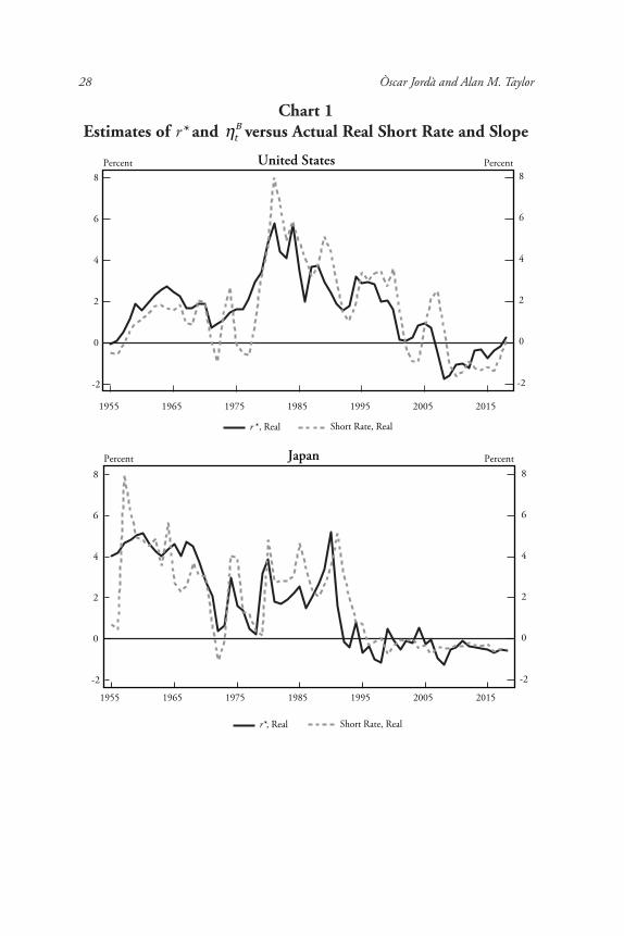
The key output from the state space model is presented in Chart 1. The figures cover the four major advanced economies and the years 1955 to 2018. Four series are shown. In the first four panels of Chart 1, one of the series is raw data, namely the real bill rate, defined as the short-term bill rate minus expected trend inflation, π t t −1
* , which is what we defined as the ex-ante real rate r. The other is the corre-sponding latent state variable estimated in the model, the real natural rate r*. The real natural rate for the four countries displays a striking common pattern over most of the sample. It reaches a local maxi-mum around 400-500 basis points (bps) in the 1980s and a global minimum around minus 100-200 bps in the last decade. The main outlier is Japan, which briefly has an even higher estimated natural rate in the 1950s, and which then drops quickly up to 1970.
For the other countries the natural rate starts low, near zero, and then for all four countries the natural rate increases sharply from the 1970s to the 1980s. In all cases the path of the natural rate broadly tracks the path of the short-term real bill rate, but does so along a much smoother path, as is expected given the parameters of the state-space model.
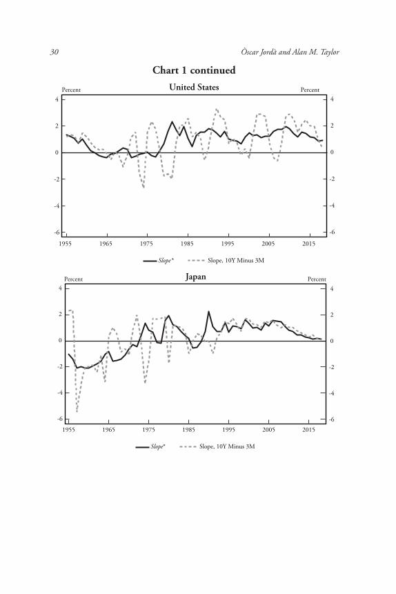
On the last four panels of Chart 1, one of the series is raw data, namely the observed term premium or slope, defined as the long-term (10-year) bond yield minus the short-term (three-month) bill yield. The other is the latent state variableηt
B estimated in the model, corresponding to the low frequency variation in the slope, which we may also denote slope*. The magnitude of the variation in slope* is noticeably smaller than that seen in r*, with a range of about 200-300 bps versus 400-600 bps. The patterns are also less clear in terms of direction. Slope has risen over time in United States, U.K. and
28 Òscar Jordà and Alan M. Taylor
Chart 1Estimates of r* and ηt
B versus Actual Real Short Rate and Slope
-2
0
2
4
6
8
-2
0
2
4
6
8
1955 1965 1975 1985 1995 2005 2015
United StatesPercent Percent
r *, Real Short Rate, Real
-2
0
2
4
6
8
-2
0
2
4
6
8
1955 1965 1975 1985 1995 2005 2015
JapanPercent Percent
r*, Real Short Rate, Real

Riders on the Storm 29
Chart 1 continued
-2
0
2
4
6
8
-2
0
2
4
6
8
1955 1965 1975 1985 1995 2005 2015
GermanyPercent Percent
r*, Real Short Rate, Real
-2
0
2
4
6
8
-2
0
2
4
6
8
1955 1965 1975 1985 1995 2005 2015
Great BritainPercent Percent
r*, Real Short Rate, Real
30 Òscar Jordà and Alan M. Taylor
-6
-4
-2
0
2
4
-6
-4
-2
0
2
4
1955 1965 1975 1985 1995 2005 2015
United StatesPercent Percent
Slope* Slope, 10Y Minus 3M
-6
-4
-2
0
2
4
-6
-4
-2
0
2
4
1955 1965 1975 1985 1995 2005 2015
JapanPercent Percent
Slope* Slope, 10Y Minus 3M
Chart 1 continued

Riders on the Storm 31
-4
-2
0
2
4
−4
−2
0
2
4
1955 1965 1975 1985 1995 2005 2015
GermanyPercent Percent
Slope, 10Y Minus 3MSlope*
−4
−2
0
2
4
−4
−2
0
2
4
1955 1965 1975 1985 1995 2005 2015
Great BritainPercent Percent
Slope, 10Y Minus 3MSlope*
Notes: Authors’ calculations. See text.
Chart 1 continued

32 Òscar Jordà and Alan M. Taylor
Japan, has drifted down in Germany, and been quite volatile in the U.K. Specifically, since 1980, the era in which estimates of r* based on short rates have collapsed dramatically by several hundred basis points, we see little sign that any strongly different trend has been seen at the long end of the yield curve.
III.ii. Decomposing the Drivers of r*
The state-space model also permits us to look under the hood and explore the drivers of the shifts in the real natural rate. Equation (6) states that rt* = zt + gt , so the real natural rate is the sum of the latent trend factor z
t and the growth rate of potential output. Chart
2 displays this decomposition for the four economies. Again, some very broad commonalities in trends stand out, after we look past the high-frequency changes. The rise and fall of the natural rate is now seen to be the combination of two patterns which are superimposed, one a downtrend, the other an inverse-U trend.
The first pattern we can make out is the gradual secular downtrend in the growth component g
t , which has been a global factor common
to all of the advanced economies in the post-World War II period. This downtrend, as expected, was strongest in Japan and Germany, where the immediate postwar growth surges had been the most rapid. In the United States and Britain, the downtrend was more gradual. The second pattern is the rise and fall of the latent factor z
t , which
captures all other secular changes in the non-growth related drivers of the natural rate in this period, such as, the well-documented greying of the population and the large fiscal consolidation post-World War II. These factors interact with each other to produce the inverted U-shape that we report. The latent factor rises 400-500 bps up to the 1980s, before turning around and, in all cases bar Japan, retracing to something close to its former level by now.
Summing up, the natural rate reached a local peak around 500 bps (±100 bps) in the mid-1980s, maybe a little lower at around 300 bps in Japan. Since then, it has fallen gradually to levels in the range of minus100 bps to 0 bps today, reaching minima even further below zero in the years right after the global financial crisis. In all countries the long-run decline is driven by a combination of drops in potential growth rate and the rise and fall of the latent factor.

Riders on the Storm 33
Chart 2The Natural Rate r*, Growth Component g and Latent Factor z
−5
0
5
10
−5
0
5
10
1955 1965 1975 1985 1995 2005 2015
United StatesPercent Percent
Natural Rate (r*), Real Latent Component (z), Real Growth Component (g), Real
−5
0
5
10
−5
0
5
10
Percent Percent
1955 1965 1975 1985 1995 2005 2015
Japan
Natural Rate (r*), Real Latent Component (z), Real Growth Component (g), Real

34 Òscar Jordà and Alan M. Taylor
–5
0
5
10
–5
0
5
10
1955 1965 1975 1985 1995 2005 2015
GermanyPercent Percent
Natural Rate (r*), Real Latent Component (z), Real Growth Component (g), Real
−5
0
5
10
−5
0
5
10
1955 1965 1975 1985 1995 2005 2015
Great BritainPercent Percent
Natural Rate (r*), Real Latent Component (z), Real Growth Component (g), Real
Notes: Authors’ calculations. See text.
Chart 2 continued
Riders on the Storm 35
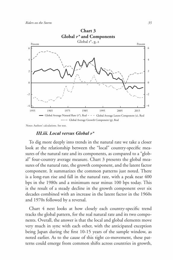
III.iii. Local versus Global r*
To dig more deeply into trends in the natural rate we take a closer look at the relationship between the “local” country-specific mea-sures of the natural rate and its components, as compared to a “glob-al” four-country average measure. Chart 3 presents the global mea-sures of the natural rate, the growth component, and the latent factor component. It summarizes the common patterns just noted. There is a long-run rise and fall in the natural rate, with a peak near 400 bps in the 1980s and a minimum near minus 100 bps today. This is the result of a steady decline in the growth component over six decades combined with an increase in the latent factor in the 1960s and 1970s followed by a reversal.
Chart 4 next looks at how closely each country-specific trend tracks the global pattern, for the real natural rate and its two compo-nents. Overall, the answer is that the local and global elements move very much in sync with each other, with the anticipated exception being Japan during the first 10-15 years of the sample window, as noted earlier. As to the cause of this tight co-movement, these pat-terns could emerge from common shifts across countries in growth,
Chart 3Global r* and Components
Global r*, g, z
Notes: Authors’ calculations. See text.
−4
−2
0
2
4
6
−4
−2
0
2
4
6
1955 1965 1975 1985 1995 2005 2015
Percent Percent
Global Average Natural Rate (r*), Real Global Average Latent Component (z), RealGlobal Average Growth Component (g), Real

36 Òscar Jordà and Alan M. Taylor
Chart 4Local versus Global r* and Components
Notes: Authors’ calculations. See text.
-2
0
2
4
6
1955 1965 1975 1985 1995 2005 2015
A. Global v Local r*
-6
-4
-2
0
2
4
1955 1965 1975 1985 1995 2005 2015
B. Global v Local z Component
0
2
4
6
8
10
-2
0
2
4
6
-6
-4
-2
0
2
4
0
2
4
6
8
10
1955 1965 1975 1985 1995 2005 2015
C. Global v Local g Component
Global Average United States Great Britain Japan Germany
Percent Percent
Percent Percent
Percent Percent
in demographics, or in financial liberalization; they could also derive from international arbitrage; or indeed from a combination of some or all these forces, depending on the era.
A longer sweep of financial history sets the post-World War II re-cord of the natural rate in a broader context. Despite much wringing of hands about the three-decade decline in the natural rate, Jordà, Knoll, Kuvshinov, Schularick and Taylor (2019) show that low real rates of return in safe asset classes occupy long stretches of time
Riders on the Storm 37
historically, in a manner consistent with a low neutral real rate of interest. If anything, it is then the relatively high levels of the real interest rates experienced in the 1980s, the very noticeable peak seen here and in other recent studies, which stand out more as the excep-tion than the rule.
IV. ‘Terrestrial’ versus ‘Celestial’ Navigation: Charting the Course of Monetary Policy
The discussion so far has emphasized a primary output of the mod-el, the natural real rate. This variable has been the focus of the many analyses using these kinds of state-space models. But this is not our only focus, since the model also generates other estimates of great interest which should provide insights into the drivers of policy, lo-cal macroeconomic dynamics, and international adjustment. In the last two sections of this paper, we turn to an examination of these features, to see if the models shed light on some of the central policy questions of the day.
To frame the discussion, it is worth emphasizing how the model allows us to decompose local monetary policy settings into three dis-tinct components. We have already discussed the “global” factor of the natural rate, what we now refer to as the “world level” of r*, which we shall denote rw*. Without loss of generality, one can write the local short-term interest rate in any economy as the sum of three terms:
rt = rt − rt*( )Stance in
local economy
!"# $#+ rt* − rW,t
*( )Local minus world
natural rate
! "# $#+ rW,t
*
Worldnatural rate
!.
(11)
Of course, in this framework, from the point of view of the local policymaker only the first of these terms, stance, is under their con-trol. In contrast, the last two terms, the path of local economy’s natu-ral rate and its deviation from the world average, are taken as given by the policymaker.3 The decomposition in equation (11) provides a useful sextant with which to measure what factors have in fact been

38 Òscar Jordà and Alan M. Taylor
driving monetary policy, and especially how much of a role the “star” terms play.
We embrace a crude dichotomy. Under what we may term the terrestrial navigation view, policymakers have their heads down. In the short run, the stars don’t move much. With eyes mainly on the ground, policymakers are guided by the local landmarks of output gaps and inflation gaps and set stance accordingly, ignoring the local and global star terms. Here, it is stance as measured by the first term in (11) that matters most.
A focus on stance as the key driver of monetary policy setting un-derpins, for example, the benchmark empirical models of interest-rate rules (e.g., J. Taylor 1993), and the canonical theory which ratio-nalizes them (e.g., Woodford 2003). In baseline versions, the policy rule intercept is constant, and by construction variations in the nat-ural rate play virtually no role, a very strong assumption but one that is occasionally put forward all the same (Wieland 2018). This view is soundly rejected by the data in our model. Our time-varying neutral rate is imprecisely estimated, but it results in a vast improve-ment of the log likelihood relative to that of a model that permits for only small fluctuations of the neutral real rate around a constant. We might say that the stars have statistical significance.
Next, consider a celestial navigation view, where policymakers would expand the horizon and would consider not simply the first term in equation (11) but the role played by the latter two terms as well. The stars are moving and must be tracked lest undesirable de-viations in the policy path accumulate and take us off course. In the terminology of Powell (2018), policymakers are not fixated only on local landmarks, but take into account the stars—that is, the local and world natural rates. This is a key augmentation to the standard models and theories, and it has been emphasized by a long literature since Laubach and Williams (2003).
Indeed, we will find that most of the variation in the policy set-tings, as measured by interest rates at the short end, is driven not by the path of the stance term but rather by changes in the paths of local r* and world r* terms in equation (11). In this sense, interest

Riders on the Storm 39
rate setting is driven by factors outside policymakers’ control. Taking the long view, the celestial matters as much if not more than the ter-restrial. The stars also have quantitative significance.
IV.i. Looking to the Stars: Variance Decomposition of Interest Rates
Are central bankers stargazers or shoegazers? This is an empirical question, and our state space model combined with the above de-composition gives us an opportunity to put to a test the terrestrial and celestial navigation views. We take a simple approach. We com-pute all terms in equation (11) for our full sample and for all four economies. We then calculate the variance of the left-hand side, and the variance of the three terms on the right-hand side, plus a re-sidual term which accounts for covariance components. The results are shown in Chart 5, for the full sample of all years, and three sub-sample periods, and provide a very clear answer.
The figure shows the variance of the first term, representing stance, in blue shaded bars. In all years this term accounts for at most about 40% of the total variance in the short rate. By comparison, the other two terms, the “star” terms, whose variance is depicted by the red and orange bars, account for almost all of the remaining 60% of the variance in the short rates.
There is variation by subperiod, but not so much as to overturn the basic point. Stance variation explains a greater share during the middle period of more erratic monetary policy from the collapse of Bretton Woods (1974) to the era of inflation targeting (1994). Not surprisingly, the more monetary policy is rudderless, in this setup, the greater action will be attributed to the use of local guidance (even if it is poor guidance) than to the slow-moving natural rate components.
Summing up, using our empirical approach, postwar history offers a very definitive judgement on the terrestrial versus celestial debate. Local and world natural rates are not constant, and their ineluctable drift pulls on the course settings of monetary policy makers, perhaps more than has been yet realized. Over five decades, a majority of short-rate variation has been driven by these star factors, and less than half by changes in the residual stance measure.

40 Òscar Jordà and Alan M. Taylor
But this variance decomposition is only a starting point for our analysis. We can do much more with the decomposition in equation (11), and the rest of the paper carries this forward in several direc-tions. In the last part of this section we look at the time variation in the dispersion of stance and how it relates to time variation in the dispersion of the real fundamental, the output gap. The uneven his-torical patterns we find are illuminating. Then in the remainder of the paper we look at the stance and star terms and study their contri-bution to macroeconomic adjustment dynamics. Providing a further cross-check on our model output, this exercise shows that both sets of terms generate adjustment predictions that align with textbook macroeconomic intuition.
IV.ii. Steering in Erratic Currents: Comparing the Evolution of Monetary Policy Stance and the Output Gap Over Five Decades
In light of the above decomposition, and as a sense check, consider the evolution of stance and gap in the four countries since 1960, dis-carding the prior five years as training data for the model given the apparent instability of some estimates in those years.
0
1
2
3
4
5
0
1
2
3
4
5
1955-1974 1975-1994 1994-2015 All years
r – r* Otherr* – r*wr*w
Chart 5Variance Decomposition of Real Short-Term Interest Rates
over Five Decades
Notes: Authors’ calculations. See text. Other refers to the residual due to covariance terms.

Riders on the Storm 41
-4
-2
0
2
4
−4
−2
0
2
4
−4
−2
0
2
4
1960 1970 1980 1990 2000 2010 2020
A. Gap Levels
-4
-2
0
2
4
1960 1970 1980 1990 2000 2010 2020
B. Stance Levels
0
5
10
15
20
0
5
10
15
20
1960 1970 1980 1990 2000 2010 2020
C. Inflation Levels
Min/Max Average
Chart 6Dispersion of Monetary Policy Stance, Output Gap and Inflation
Notes: Authors’ calculations. See text. Smoothed estimates in lower panel use a bandwidth of eight years.
42 Òscar Jordà and Alan M. Taylor
0.5
1.0
1960 1970 1980 1990 2000 2010
0.5
1.0
1.5
2.0
2.5
1960 1970 1980 1990 2000 2010
2
4
6
2
4
6
1960 1970 1980 1990 2000 2010
sd
E. Stance Dispersion
F. Inflation Dispersion
Smooth Line of Estimates
D. Gap Dispersion
0.5
1.0
0.5
1.0
1.5
2.0
2.5
Chart 6 continued
Notes: Authors’ calculations. See text. Smoothed estimates in lower panel use a bandwidth of 8 years.

Riders on the Storm 43
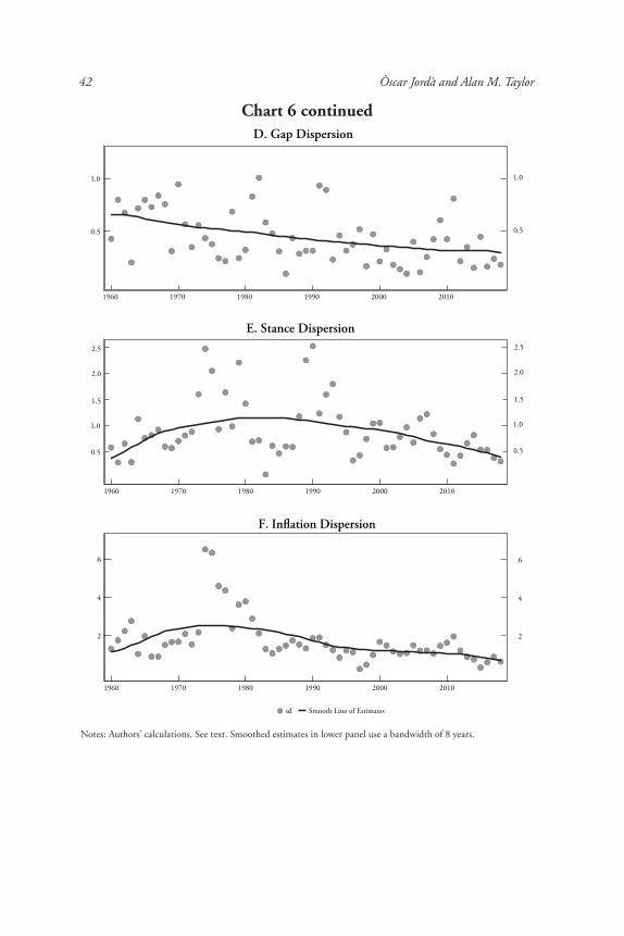
Chart 6 presents descriptive summaries of the model estimates. For now, we will focus on the figures in the first and second panels, referring to gap and stance. We then will discuss inflation dispersion behavior, described by the figures in the bottom three panels. The figures show the average levels of stance and gap in the four-country sample, along with an indication of the min-max range in each year to show the dispersion. Next is an alternative measure of dispersion, the standard deviation of gap and stance, by year, with a nonpara-metric estimated trend based on a kernel regression also shown.
These figures summarize two important but contrasting trends in the key model-implied state variables, stance and gap, in the last 60 years. With respect to gap, the cross-country dispersion has seen on a long, gradual, monotonic downward trend for the last six decades, al-lowing for some short-run volatility along the way. The business cycles of the four economies have steadily moved into greater synchroniza-tion over time. This happened even as potential output followed rather different paths (Japan versus the United States, for example). It is a striking feature and, a priori, it is not obvious why this would be so. Looking at the trend, gap dispersion is now at about half of its level in 1960. Even in the absence of explicit monetary policy coordination, and in light of this degree of business cycle synchronization, one would expect monetary policy stance to be similarly synchronized.
However, this does not appear to be quite the case. The trend is hump shaped. For the first two or three decades, even as the real economies became more aligned, monetary policy stance got ever more divergent in these economies. The finding is intuitive and fits the historical narrative: with Bretton Woods falling apart, central banks groped for a new nominal anchor, but they blundered about for 10 or 20 years before they all coalesced on a new inflation-target-ing consensus, and that new policy regime eventually brought stance dispersion more closely back into line with gap dispersion.
The dispersion in output gaps has been declining throughout the post-World War II era, even before the start of the period commonly referred as the Great Moderation. Interestingly, the dispersion in mon-etary policy stances, measured as the deviation of the real rate from the neutral rate, does not quite fit the same pattern. Today stance

44 Òscar Jordà and Alan M. Taylor
dispersion is also at about one half of its level in 1960, but it took a much more interesting journey along the way. But as of now, from the perspective of the full post-World War II experience, the current ob-served divergence in stance appears well within the historical norm.
This narrative is consistent with the final three panels in Chart 6. While gap dispersion was falling in a more or less straight line, the central banks in our sample lost control of inflation in the 1970s, to greater or lesser degrees. One could say that the mistakes derived from large shifts in policy stance as inflation control went out of kilter, and the correction of the mistakes subsequently allowed a con-quest of inflation globally, but this required further large shifts in policy stance, to get inflation control back on track. Thus, stance and inflation left a very volatile signature in these records in the middle years, even as real side volatility due to gap followed a calm and grad-ual descent from start to end.
V. Policy Stance, the Business Cycle and Domestic Adjustment
In this section, we will first explore what the model outputs have to say about standard theories of the domestic co-evolution of the first term above, stance
t ≡ rt ‒ rt
* , and its natural co-state variable, gap
t ≡xt ≡ yt ‒ yt
*, which measures the distance between actual and potential output. In the next section we ask how the first term, the dif-ferential between local and world natural rates relates to theories of the international adjustment process. To start, a simple Granger causality ap-proach confirms intuition about how policy affects the state of the econ-omy, and how policy is in turn influenced by the state of the economy.
V.i. The Dynamics of Stance and Gap
Given the model implied stance and gap measures, we investigate their co-evolution in a small-scale estimated dynamical system. We estimate reduced-form local projections of future cumulative chang-es in a vector Δh yi,t= yi,t+h- yi,t-1, where the vector elements are y = {stance, gap}, and outcomes are changes from year t –1 to t +h, regressed on observed changes in stance and gap in year t, denoted Δ yi,t , plus two lags of the state vector as additional controls xi,t. Esti-mation of each equation is by panel OLS with country fixed effects.

Riders on the Storm 45
Table 1LP Dynamics of Stance and Gap, Four-Country Panel
rt+3 − rt+3*
Δ(yt − yt* ) 0.44**
(0.11) 0.27**(0.13)
‒0.15(0.14)
‒0.16(0.14)
Δ(rt– rt* ) 0.55**
(0.07)0.16**
(0.08) 0.12(0.08)
0.01(0.08)
N. obs 244 240 236 232
yt+3 − yt+3*
Δ(yt − yt* ) ‒0.02
(0.07) ‒0.51**(0.04)
‒0.20(0.09)
0.01(0.04)
Δ(rt– rt* ) ‒0.12*
(0.04)‒0.11**(0.03)
0.02(0.05)
0.02(0.03)
N. obs 244 240 236 232
rt+4 − rt+4*
rt+4 − rt+4*
rt+2 − rt+2*
yt+2 − yt+2*
rt+1 − rt+1*
yt+1 − yt+1*
A. Response of Stance to Changes in Gap and Stance
B: Response of Gap to Changes in Gap and Stance
* p<0.10** p<0.05Notes: Authors’ calculations. See text. Standard errors in parentheses.
Do these predictive estimates accord with intuition? Table 1 sug-gests that they do. Panel A displays the response of stance to gap and to itself. The response of stance to gap is significant at the one- and two-year horizons and has the expected positive sign. An increase in gap, i.e., a more rapidly growing economy, predicts a tighter policy stance one year ahead. Beyond one year all estimates are small. The own response of stance to itself is moderately persistent, but also has the expected sign. After one year about 60% of the change in stance persists, the largest response coefficient of the four. In future years, stance is then predicted to revert. Beyond one year all estimates are again small.
Panel B displays the response of gap to itself and to stance. The own response of gap to gap shows the typical mean reversion pat-tern. Unusually high growth today in general predicts lower growth going forward. The response of gap to stance shows the conventional results: a monetary policy contraction today leads to a more negative
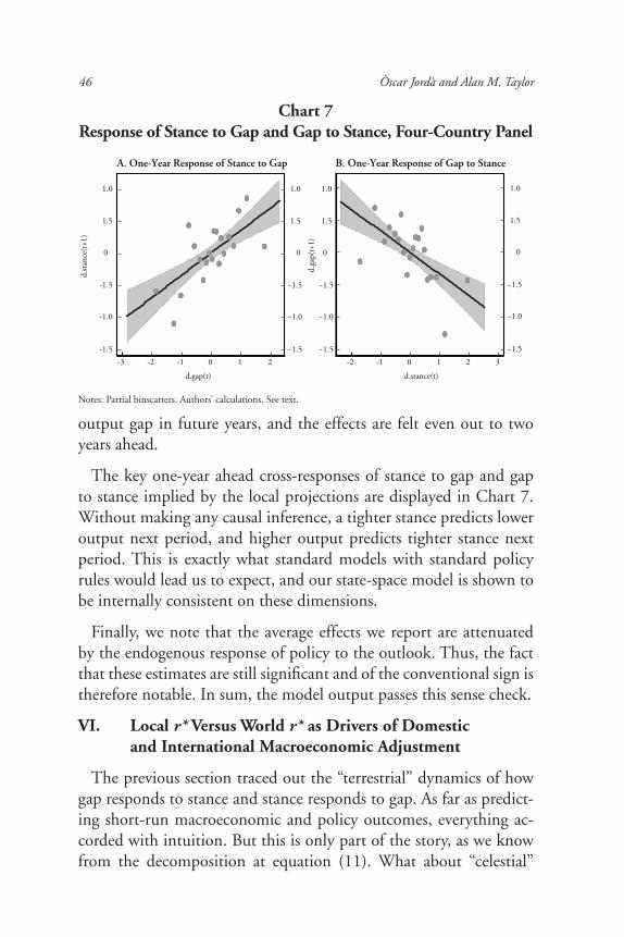
46 Òscar Jordà and Alan M. Taylor
output gap in future years, and the effects are felt even out to two years ahead.
The key one-year ahead cross-responses of stance to gap and gap to stance implied by the local projections are displayed in Chart 7. Without making any causal inference, a tighter stance predicts lower output next period, and higher output predicts tighter stance next period. This is exactly what standard models with standard policy rules would lead us to expect, and our state-space model is shown to be internally consistent on these dimensions.
Finally, we note that the average effects we report are attenuated by the endogenous response of policy to the outlook. Thus, the fact that these estimates are still significant and of the conventional sign is therefore notable. In sum, the model output passes this sense check.
VI. Local r* Versus World r* as Drivers of Domestic and International Macroeconomic Adjustment
The previous section traced out the “terrestrial” dynamics of how gap responds to stance and stance responds to gap. As far as predict-ing short-run macroeconomic and policy outcomes, everything ac-corded with intuition. But this is only part of the story, as we know from the decomposition at equation (11). What about “celestial”
Chart 7Response of Stance to Gap and Gap to Stance, Four-Country Panel
-1.5
-1.0
-1.5
0
1.5
1.0
−1.5
−1.0
−1.5
0
1.5
1.0
−1.5
−1.0
−1.5
0
1.5
1.0
−1.5
−1.0
−1.5
0
1.5
1.0
d.sta
nce(
t+1)
-3 -2 -1 0 1 2
d.gap(t)
d.ga
p(t+
1)
-2 -1 0 1 2 3
A. One-Year Response of Stance to Gap B. One-Year Response of Gap to Stance
d.stance(t)
Notes: Partial binscatters. Authors’ calculations. See text.

Riders on the Storm 47
forces, and how they interact with macroeconomic outcomes? In this section we turn to the star terms and examine how shifts in these non-policy variables predict medium term macroeconomic adjust-ment to fundamentals.
The gap between local and world natural rates may sit outside lo-cal policymakers’ control, but according to standard theory it should have a very important influence on local economic outcomes via the international adjustment process. Since our model-implied estimates give us a way to measure the gap between local and world natural rates, we are in a position to ask whether empirically, over the long run, the evidence supports this view of how the mechanisms of inter-national adjustment actually work.
Naturally, this requires a transition to an open economy frame-work. Again, we eschew formal models, but we ground our thinking using the ideas presented in Clarida (2019). That paper, following Clarida, Galí and Gertler (2002), explores policy in a two-country DSGE model with global and country-specific r* shocks which are a function of productivity only, as well as cost push shocks. Clarida (2019) maps from the model to the empirical effects seen in Holston, Laubach and Williams (2017) four individual country estimates us-ing a vector error correction model (VECM) of the natural rate. In this idealized model, global and local r* shocks must both pass through into the local policy rate under optimal policy.4
A notable feature of the setup is that, if the natural rate is observed perfectly in real time, the central bank can replicate the flexible price equilibrium by passing through the natural rate shock fully and imme-diately to the policy rate. In more realistic settings, and as we see in the data, the pass-through is likely to be gradual, perhaps justified by the signal extraction problem if the natural rate is known only with noise. In those more realistic circumstances, under a gradual incorporation of real rate shocks into the policy rate, several patterns should be expected. A hypothesized positive productivity shock to the local r* will be accom-panied by a boom in output and inflation that persists, but the strong economy will eventually be tempered by a rising real policy rate. On the way, the local stance—the difference between natural and observed real rates, will be elevated, and consequently the local currency should be
48 Òscar Jordà and Alan M. Taylor
expected to appreciate, another adjustment channel. We might ask, giv-en our model outputs: Is this actually the case in the data?
We think it is of interest to ask what other statistical signatures a natural rate shock might leave in the data, and the current account identity stands out as a natural nexus of international adjustment. In the Clarida (2019) model, this channel is shut down by log prefer-ences (cf. Cole and Obstfeld 1991), but in general we expect nontriv-ial responses of saving, investment and the current account. Along these lines, Obstfeld (2019) proposes that the economy with the higher (lower) autarky natural real rate would run a current account deficit (surplus) in the open economy equilibrium until equilibration occurs. In the case of a productivity-led shock to the home natural rate, with gradual adjustment to equilibrium, we would expect the current account to move toward deficit and the real exchange rate to appreciate endogenously. In many canonical models, without capital, this would be achieved via consumption adjustment, but where capi-tal is present, a productivity-led rise in the home natural rate might be expected to stimulate higher investment also.
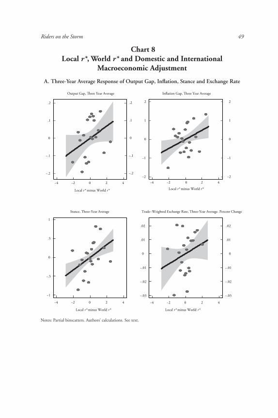
Our aim here is to undertake a preliminary and only informal em-pirical assessment of these mechanisms by presenting some suggestive correlations based on the output of our state-space model. We now know that local and global natural rates track together in the long run, but local-global differentials clearly do open up quite frequently when, from time to time, local and global shocks differ. We therefore condition on local-world natural rate differentials and see if they can forecast macroeconomic outcomes looking forward. As a first pass, we again utilize a local projection framework, but now with an eye to medium term adjustment dynamics. Thus, the outcome variable is the average response over three years. The treatment variable is the gap between local and world levels of the natural rate. These experi-ments are reported in Chart 8.
Firstly, panel A shows the predicted response of the output gap, inflation gap, stance, and the (trade-weighted) exchange rate to the local-world natural rate differential. From equation (4), as just noted, unless stance adjusts instantly, a higher local natural rate will be associ-ated with output exceeding potential going forward, a strong or hot
Riders on the Storm 49
Chart 8Local r*, World r* and Domestic and International
Macroeconomic Adjustment
−.2
−.1
0
.1
.2
−.2
−.1
0
.1
.2
−4 −2 0 2 4
−2
−1
0
1
2
−2
−1
0
1
2
−4 −2 0 2 4
Output Gap, �ree Year Average Inflation Gap, �ree Year Average
Local r* minus World r* Local r* minus World r*
−1
−.5
0
.5
1
Stance, Three-Year Average
−4 −2 0 2 4
−.03
−.02
−.01
0
.01
.02
Trade−Weighted Exchange Rate, Three-Year Average. Percent Change
−4 −2 0 2 4
Local r* minus World r*Local r* minus World r*
−.03
−.02
−.01
0
.01
.02
Notes: Partial binscatters. Authors’ calculations. See text.
A. Three-Year Average Response of Output Gap, Inflation, Stance and Exchange Rate

50 Òscar Jordà and Alan M. Taylor
B. Three-Year Average Response of Current Account, Saving, Investment and Credit
Chart 8 continued
–2
–1
0
1
2
Current Account/GDP, Three Year Average
–4 –2 0 2 4
Local r* minus World r*
–2
–1
0
1
2
–2
–1
0
1
2
–2
–1
0
1
2
Saving/GDP, Three-Year Average
–4 –2 0 2 4
Local r* minus World r*
–.02
–.01
0
.01
.02
–.02
–.01
0
.01
.02
Investment/GDP, Three-Year Average
–4 –2 0 2 4
Local r* minus World r*
–.05
0
.05
.1
–.05
0
.05
.1
Real Loans, Three-Year Average. Percent Change
–4 –2 0 2 4
Local r* minus World r*
Notes: Partial binscatters. Authors’ calculations. See text.

Riders on the Storm 51
economy. Then, from equation (7) this will feed into higher infla-tion. Subsequently, as policy adjusts, stance should tighten, and the exchange rate should strengthen. The figures show that in the data the sign of all four responses accord with this logic. Judged here, the state-space model fares well in matching key macro variables of interest.
Secondly, panel B shows the response of the various flow measures to the local-world natural rate differential. From theory we expect that a higher local natural rate, all else equal, would predict higher current account deficits in future, and this is very strongly the case in the data, with a positive correlation between CA/GDP ratios and the r* differential. We see that this response is partly driven by a decline in local saving/GDP ratios, and a rise in local investment/GDP ratios.
All responses are consistent with standard economic logic. Relat-edly, the final chart shows that the higher CA deficit, lower saving and higher investment responses are mediated by a period of stronger growth in real credit growth in the local economy. Of course, this credit boom response brings to mind the concerns noted by Obstfeld (2019) that these shocks may well have financial stability as well as monetary policy implications.5 These responses accord with an in-vestment channel that runs through credit markets, and so on this di-mension the output of the state-space model also appears reasonable.
VII. Conclusion: Implications for Monetary Policy
What lessons should policymakers draw from our analysis? It is worth reflecting on what theoretical economic models tell us first. On one side, Corsetti, Dedola and Leduc (2010) argue that, out-side the laboratory of frictionless economies, incomplete exchange-rate pass-through and asset market imperfections (to name just two potential frictions) generate distortions and spillovers that justify greater international monetary policy cooperation. But such coop-eration requires optimal domestic policy to incorporate international elements that distort the optimal domestic response under monetary autarky. As Clarida (2019) argues persuasively, such short-run distor-tions can be perceived by the public as running counter to domes-tic interests and hence undermine the credibility of domestic central
52 Òscar Jordà and Alan M. Taylor
banks, the cornerstone on which modern central banking rests. And credibility is particularly valuable now that low neutral real rates of interest are likely to limit traditional interest rate policy in favor of nontraditional monetary tools, including forward guidance, whose effectiveness rests squarely on credibility.
Theory provides a disciplining device to think through the conse-quences of alternative scenarios in an organized manner. But, in the end, whether one point of view or another is closer to the mark comes down to the empirical evidence. In this paper we step away from try-ing to arbitrate how much central bank cooperation there should be. Rather, we think it is more useful to first document the reality of how much policy divergence there is in the data currently, and in the past, and to explore its sources and potential consequences.
As we discussed earlier, measuring divergence by directly comparing interest rates across economies is a coarse and atheoretical approach. As the decomposition in equation (11) showed, interest rates can fluctu-ate due to the monetary policy stance (i.e., deviations from the neutral rate of interest), and deviations of the domestic neutral rate from the global neutral rate. The latter is the international equilibrium rate an-choring all other rates. In a world with perfect capital mobility and risk sharing, this would be the equilibrium rate of interest that would prevail everywhere. The bottom line is that, in the short run, only the stance is under the control of the monetary authority.
Estimates based on our model suggest that the current divergence in neutral rates of interest is well within the historical norm. And this is true for its components as well: the rate of potential growth, and the latent drivers of the neutral rate (a holding tank for a variety of other drivers of the neutral rate, such as demography, fiscal policy, financial development, and so on), something that had not always been the case in earlier periods. In fact, the evidence provided in Chart 4 indicates that over the post-World War II era, the growth and latent components of the domestic neutral rate are in greater synchrony today than at any time in the past.
Riders on the Storm 53
Digging deeper into each component and the monetary policy stance in particular, Chart 6, panel E suggests that divergence in the policy stance has gradually declined over the past six decades and is now at its lowest point. And this is happening at the same time as the business cycle has become increasingly synchronized, as Chart 6, panel D shows.
Returning to the second major component of interest rates, the gap between the domestic and the global neutral real rate of interest, Chart 8 provides a clear reminder that this gap has important conse-quences for the international adjustment of key variables. As the ba-sic correlations in that chart show, the more the domestic neutral rate diverges from the global, the bigger the impact on exchange rates, the current account and credit flows down the road. As Obstfeld (2019) explains, persistent current account imbalances can be the canary in the coal mine that warns of impending imbalances in credit markets and thus an elevated risk of financial fragility.
Finally, two thoughts on broader policy implications.
First, the neutral rate gap shows up in important ways that are relevant to understanding current economic conditions. As Chart 8 shows, variation in the neutral rate gap shows up on inflation and the output gap. Thus, a central banker grappling with persistently low inflation must consider the possibility that the domestic neutral rate has dropped and that the monetary stance needs to be accordingly adjusted, even when there is considerable uncertainty about where the neutral rate really lies.
Second, the long real rate has tracked down fairly consistently with the short real rate over recent decades. The latent factor slope* tells this story. Our estimate of this low-frequency term premium com-ponent is still positive, albeit smaller in Japan and Germany (<100 bps) and larger in the United States and U.K. (150–200 bps). This has implications for unconventional monetary policy, since a smaller term premium, all else equal, reduces the policy space for large scale asset purchases aimed at shifting the yield curve.

54 Òscar Jordà and Alan M. Taylor
VII.i. Caveat: Can Policy Affect the Neutral Rate?
Standard theory says money is neutral in the long run. A central bank cannot use monetary policy to generate growth, only mitigate short-run fluctuations. It has no influence on the neutral rate. This is the position we adopt in this paper. Since the global financial crisis, however, this canon has been challenged from a variety of corners. Re-covery from the financial crisis and the European sovereign crisis has been disappointing. Real output is not returning to pre-crisis trends, a considerable loss of welfare with social and political ramifications all too apparent. Summers (2016) argued that we may be in an era of secular stagnation, with chronic excess of saving over investment that can be best sorted by boosting public investment. Tight fiscal policy when the neutral rate is low can have contractionary spillovers (Krug-man 2013; Setser 2019; Fornaro and Romei forthcoming).
Meanwhile, some research raises the possibility that monetary policy does in fact have important consequences for the potential rate of economic growth. Bernanke and Mihov (1998) provided em-pirical evidence of the long-lasting effects of monetary shocks. At least since Stadler (1990), business cycle models with endogenous technology justify why productivity growth can be amplified or at-tenuated depending on whether the economy is in a boom or a bust: R&D investment is closely linked with the business cycle. Recent work by Jordà, Singh and Taylor (2019) finds evidence to support this view. Such mechanisms paired with the current macroeconomic outlook and low or negative neutral real rates of interest, suggest that monetary policy could indeed have long-run effects on the neutral rate of interest. Tight local or global policy stance could lead to long-run persistent downturns in the neutral real rate.6 In such a scenario, the internally consistent picture we have painted might need to be redrawn considerably.
VII.ii. Final Thoughts
The global financial crisis left a heavy imprint in the economic landscape. The seeds for greater policy divergence planted by the crisis sprouted on both sides of the Atlantic and the Pacific in the past few years. Anxieties about the negative spillovers and stresses that non-coordinated policy divergence might place upon the system

Riders on the Storm 55
have become apparent. Talk of currency wars and exchange rate ma-nipulation started to make headlines.
Yet without firmer empirical evidence, of the kind we present here, it is difficult to know how concerned we should be. And our argu-ment that long-run forces matter, that these forces are beyond policy-makers’ control, and also contain a strong global component, could support a more benign narrative.
We stress that a direct comparison of interest rates across coun-tries is too coarse a measure of monetary policy divergence or lack of monetary policy coordination. We show that the monetary policy stance only makes sense in reference to the neutral rate prevailing in the economy. In addition, an economy’s neutral rate cannot diverge from the global neutral rate given the levels of real and financial inte-gration characterizing modern economies.
A central bank has a duty to protect the economic and financial welfare of its citizens. In a globalized economy with low rates of growth, low neutral real rates of interest, and tight financial integra-tion, carrying out that duty will inevitably require central banks to adopt a global perspective.
Authors’ Note: For their most helpful comments we thank Ben Bernanke, Ol-ivier Blanchard, Pierre-Olivier Gourinchas, Andrew Haldane, Maurice Obstfeld, Łukasz Rachel, Moritz Schularick, Sanjay Singh and Lawrence Summers. All er-rors are our own. The views expressed herein are solely the responsibility of the authors and should not be interpreted as reflecting the views of the Federal Reserve Bank of San Francisco or the Board of Governors of the Federal Reserve System.

56 Òscar Jordà and Alan M. Taylor
Endnotes1See the papers of Corsetti, Dedola and Leduc (2008, 2010). The former makes
the point that under special conditions, global conditions can be ignored. The lat-ter stresses that more generally this is not the case, and what then needs to be done to achieve an optimal policy.
2See, e.g., Carvahlo, Ferrero and Nechio (2016) on demographics, and Rachel and Summers (2019) on fiscal policy.
3Though some would go so far as viewing the natural rate as endogenous to monetary policy. See Borio et al. 2018.
4One interesting corollary of the model is that, under symmetry, global shocks do not pass through into exchange rates. The reason is that the equilibrium ex-change rate is a function of (transitory) PPP gaps and output gaps plus a term reflecting expected future real natural rate differentials.
5See Schularick and Taylor (2012) and Jordà, Schularick and Taylor (2013) for evidence which shows, using the same dataset, that credit booms are associated with costly financial instability.
6Note that what we describe runs counter to the causality in Borio, Disyatat and Rungcharoenkitkul (2019), who claim that a loose stance fosters endogenously lower neutral rates.

Riders on the Storm 57
References
Bernanke, Ben S., and Ilian Mihov. 1998. “Measuring Monetary Policy,” Quar-terly Journal of Economics, 113(3): 869-902.
Borio, Claudio, Piti Disyatat and Phurichai Rungcharoenkitkul. 2019. “What Anchors the Natural Rate of Interest?” BIS Working Paper 777.
Carvahlo, Carlos, Andrea Ferrero and Fernanda Nechio. 2016. “Demograph-ics and Real Interest Rates: Inspecting the Mechanism,” European Economic Review, 88: 208-226.
Clarida, Richard H. 2019. “The Global Factor in Neutral Policy Rates: Some Implications for Exchange Rates, Monetary Policy, and Policy Coordination,” International Finance Discussion Papers 1244, Board of Governors of the Federal Reserve System.
_____, Jordi Galí and Mark Gertler. 2002. “A Simple Framework for Inter-national Monetary Policy Analysis,” Journal of Monetary Economics, 49(5): 879-904.
Coibion, Olivier, Yuriy Gorodnichenko, Lorenz Kueng and John Silvia. 2017. “Innocent Bystanders? Monetary Policy and Inequality,” Journal of Monetary Economics, 88(C): 70-89.
Cole, Harold L., and Maurice Obstfeld. 1991. “Commodity Trade and Inter-national Risk Sharing: How Much Do Financial Markets Matter?” Journal of Monetary Economics, 28(1): 3-24.
Corsetti, Giancarlo, Luca Dedola and Sylvain Leduc. 2010. “Optimal Monetary Policy in Open Economies,” in Handbook of Monetary Economics, edited by Benjamin M. Friedman and Michael Woodford, 1st edition, vol. 3, chap. 16, pp. 861-933 Amsterdam: Elsevier.
_____, _____ and _____. 2008. “International Risk Sharing and the Transmis-sion of Productivity Shocks,” Review of Economic Studies, 75(2): 443-473.
Fornaro, Luca, and Federica Romei. “The Paradox of Global Thrift,” American Economic Review, forthcoming.
Galí, Jordi. 2015. Monetary Policy, Inflation, and the Business Cycle: An Introduc-tion to the New Keynesian Framework and Its Applications. 2nd edition. Princ-eton, New Jersey: Princeton University Press.
Holston, Kathryn, Thomas Laubach and John C. Williams. 2017. “Measuring the Natural Rate of Interest: International Trends and Determinants,” Journal of International Economics, 108(S1): S59-S75.
Jordà, Òscar, Sanjay Singh and Alan M. Taylor. 2019. “The Long-Run Effects of Monetary Policy,” University of California-Davis, unpublished.

58 Òscar Jordà and Alan M. Taylor
_____, Katharina Knoll, Dmitry Kuvshinov, Moritz Schularick and Alan M Tay-lor. 2019. “The Rate of Return on Everything, 1870–2015,” Quarterly Journal of Economics, 134(3): 1225-1298.
_____, and Fernanda Nechio. 2018. “Inflation Globally,” Federal Reserve Bank of San Francisco Working Paper 2018-15.
_____, Moritz Schularick and Alan M. Taylor. 2017. “Macrofinancial History and the New Business Cycle Facts,” in NBER Macroeconomics Annual 2016, vol. 31, edited by M. Eichenbaum and J. Parker. Chicago: University of Chi-cago Press.
_____, _____ and _____. 2015. “Leveraged Bubbles,” Journal of Monetary Eco-nomics, 76: S1-S20.
_____, _____ and _____. 2013. “When Credit Bites Back,” Journal of Money, Credit and Banking, 45(s2): 3-28.
King, Mervyn, and David Low. 2014. “Measuring the ‘World’ Real Interest Rate,” NBER Working Paper 19887.
Krugman, Paul. 2013. “The Harm Germany Does,” The New York Times, Nov. 1.
Laubach, Thomas, and John C. Williams. 2003. “Measuring the Natural Rate of Interest,” Review of Economics and Statistics, 85(4): 1063-1070.
Obstfeld, Maurice. 2019. “Global Dimensions of U.S. Monetary Policy,” paper presented at Monetary Policy Strategy, Tools, and Communication Practices, A Fed Listens event, Federal Reserve Bank of Chicago, June 4-5.
Powell, Jerome H. 2018. “Monetary Policy in a Changing Economy,” in Chang-ing Market Structure and Implications for Monetary Policy, Federal Reserve Bank of Kansas City, Economic Policy Symposium, Jackson Hole, Wyoming, Aug. 24-25, pp. 1-18.
Rachel, Łukasz, and Lawrence H. Summers. 2019. “On Falling Neutral Rates, Fiscal Policy, and the Risk of Secular Stagnation,” Brookings Papers on Economic Activity, Conference Draft, March 7-8.
_____, and Thomas D. Smith. 2015. “Secular Drivers of the Global Real Interest Rate,” Bank of England Working Paper 571.
Romer, Christina D., and David H. Romer. 2004. “A New Measure of Monetary Shocks: Derivation and Implications,” American Economic Review, 94(4): 1055-1084.
Schularick, Moritz, and Alan M. Taylor. 2012. “Credit Booms Gone Bust: Monetary Policy, Leverage Cycles, and Financial Crises, 1870–2008,” American Economic Review, 102(2): 1029-1061.

Riders on the Storm 59
Setser, Brad W. 2019. “Time for China, Germany, the Netherlands, and South Korea to Step Up,” Council on Foreign Relations Blog, Jan. 9, 2019. https://www.cfr.org/blog/time-china-germany-netherlands-and-korea-step
Stadler, George W. 1990. “Business Cycle Models with Endogenous Technology,” American Economic Review, 80(4): 763-778.
Summers, Lawrence H. 2016. “The Age of Secular Stagnation: What Is It and What to Do About It,” Foreign Affairs, 95(2): 2-9.
Taylor, John B. 1993. “Discretion Versus Policy Rules in Practice,” Carnegie Roch-ester Conference Series on Public Policy, 39: 195-214.
Wicksell, Knut. 1936 [1898]. Interest and Prices. English translation of 1898 edi-tion by R. F. Kahn. London: Macmillan.
Wieland, Volker. 2018. “R-star: The Natural Rate and its Role in Monetary Policy,” in The Structural Foundations of Monetary Policy, edited by Michael D. Bordo, John H. Cochrane and Amit Seru. Stanford, California: Hoover Institution Press.
Woodford, Michael. 2003. Interest and Prices: Foundations of a Theory of Monetary Policy. Princeton, New Jersey: Princeton University Press.