Rossana PasquinoPh.D. Thesis in Chemical Engineering

(XXI cycle)

Rheology of viscoelasticsuspensions

JuryProf. Nino Grizzuti, promotor

Dr. Francesco GrecoProf. Pier Luca Maffettone

Prof. Jan Vermant

Non ho particolari talenti, sono solo appassionatamente curioso.A. Einstein

1

A nonna Ninuccia

2

Acknowledgments

Mi piacerebbe poter ringraziare coloro i quali hanno contribuito in questianni al mio lavoro di tesi di dottorato.In primis vorrei ringraziare Nino (per una volta il ”tu”) per aver creduto inme fin dall’inizio (sperando che non se ne sia pentito..), per avermi inculcatol’entusiasmo della scoperta e per il supporto emotivo che non mi ha fattomai mancare.Grazie a Francesco, per le discussioni accademiche (e non), per i pianti, isorrisi, i discorsi su quotidianita e vita. Se sono migliorata, e non solo acca-demicamente (anche se non mi dirai mai di sı), buona parte del merito e suo.Grazie a Pier Luca, per non avermi mai fatto sentire la differenza tra ”il” pro-fessore e lo studente e per l’estrema disponibilita che ha sempre dimostrato.Thanks to the professor Jan Vermant, to give me the possibility to improvemy professional knowledge and to support me during my ”bad” period inBelgium. I will never forget our meetings and the words ”it’s amazing!”,that well express all your curiosity and passion for research.Grazie ai miei amici di sempre, a quelli di cui non ho mai sentito la man-canza, a quelli che ho incontrato da poco, a quelli che sono passati per pocoe mi sono rimasti sulla pelle. In particolare ringrazio Alessia, Rita, Elisa,Gustavo, Alessandro, Erman e Cettina senza cui i miei mesi a letto sareb-bero durati una eternita. Ed i ragazzi del Paolella, in particolare Luisa, chee piu di una sorella.Grazie a Ginia, per le mille telefonate e per avermi regalato il sorriso diFede.Grazie ai miei colleghi napoletani, Claudia, Stefano e Francesco e non hobisogno di spiegare perche, tutto e gia nelle intere giornate passate insieme.Thanks to Frank (the angel of my office!) for our discussions on researchand ”life’s purposes”, to be always nice and ”predictable”, to correct thisthesis...Basa (a good cook!), Naveen and Kasper without whom my expe-rience in Belgium would have had surely less importance. In particular,Basa’s rigor, integrity and curiosity serve as the standard that I shall aspireto throughout my professional life.Grazie, ancora, ad Eleonora, Anneleen and Leen per le nostre indimenticabiliserate belghe e per avermi regalato affetto incondizionato!Thanks to all the people of the ”Etna”.At last but not least, non posso che dire grazie ai miei genitori, presenzacostante, accorta, sentita. Mi hanno dedicato buona parte della loro vita,rendendomi migliore giorno dopo giorno. Sono riusciti a farmi sentire sem-pre importante, amata. Spero di poter un giorno ricambiare con lo stessointenso amore. Non avrei potuto desiderare genitori migliori.

3

Grazie, infine, ai miei fratelli, che, dovunque si trovino e mi trovi, sono erimarranno sempre ad un passo da me.

”chi car’ e s’ aiz nun e mai carut...”

4

Summary

The rheology of suspensions of solid particles in viscoelastic fluids is impor-tant in many technological applications as exemplified by the processing offilled polymers e.g. injection molding, coating processes, application in foodand health care products,...Consequently, considerable attention in the literature is given to the rheologyof suspensions of particles. Most studies are focused on highly filled systems(typically, volume fractions greater than 10%), with polydisperse particles ofirregular shapes due to their technological importance. In contrast, realtivelyfew studies are conducted on the rheology of dilute or semi-dilute suspensionsof monodisperse spheres.In the first part we elucidate the effect of viscoelasticity on the bulk rhe-ological properties. The behavior of model suspensions composed of nonBrownian, inertialess, rigid spheres immersed in Newtonian and viscoelasticmatrices is investigated in the concentration range from 0 up to 10%, thusencompassing both the dilute and semidilute regimes. The data are fittedwith quadratic polynomial functions of the particle volume fraction in orderto compare with theoretical, empirical and experimental models.As second part, new simulation technique for suspensions in Newtonian flu-ids under oscillatory shear flow is presented. The cases of a single sphere andtwo particles are studied and discussed.Finally, the flow induced microstructure of suspensions in viscoelastic flu-ids is studied by rheo-optical techniques. More specifically, the flow-inducedalignment of non-colloidal particles in viscoelastic fluids is investigated sys-tematically in an attempt to quantify the alignment of the particles andcorrelate it with the shear rate, size of the particles and interactions with thewall.

5

List of Figures

1.1 Data from Rutgers. . . . . . . . . . . . . . . . . . . . . . . . . 211.2 Data from Saunders. The slope of 6.2 is in good agreement

with Batchelor’s prediction . . . . . . . . . . . . . . . . . . . . 221.3 Normalized effective viscosity of suspensions as a function of

volume fraction of monosized hard spheres showing compari-son between Hsueh’s work and existing predictions [20]. . . . . 23

1.4 Time-averaged bulk shear viscosity as a function of solid areafraction, calculated from the single particle problem [23]. . . . 24

1.5 Relative bulk shear viscosity as a function of solid area frac-tion. Hwang and Hulsen results [24] are plotted as well (opensquares). . . . . . . . . . . . . . . . . . . . . . . . . . . . . . . 25

1.6 Relative shear viscosity as a function of solid area fraction fordifferent Weissenberg numbers [37]. . . . . . . . . . . . . . . . 28

1.7 Alignment and aggregation effects in suspension of spheres innon Newtonian fluid (a) after loading (b)with few oscillationsof the plate (c)after several oscillations (d)after long oscillatorytimes . . . . . . . . . . . . . . . . . . . . . . . . . . . . . . . . 33

1.8 Alignment of a bidisperse suspension in a non-Newtonian liq-uids [61]. . . . . . . . . . . . . . . . . . . . . . . . . . . . . . . 34

1.9 Imbalance of shear rate for two cylinders. . . . . . . . . . . . . 35

2.1 Particle size distribution for PMMA spheres. . . . . . . . . . . 392.2 Particle size distribution for glass beads. . . . . . . . . . . . . 392.3 TGA for aPP suspensions. . . . . . . . . . . . . . . . . . . . . 412.4 DFST for Newtonian Polyisobutylene, at 30C. . . . . . . . . 442.5 DFST for the Dow Silicone Fluid, at 30C. . . . . . . . . . . . 452.6 DFST for the Rhodorsil fluid, at 30C. . . . . . . . . . . . . . 452.7 The steady shear viscosity of PIB based suspensions as func-

tion of shear rate at various filler concentrations. . . . . . . . . 46

6

2.8 Loss modulus for PDMS-B based suspensions as function offrequency at various filler concentrations; (a) for all measuredfrequencies (lines are guides to the eye); (b) in the low fre-quency range: lines are linear regressions of the data). Sym-bols as in the Fig. 2.7. . . . . . . . . . . . . . . . . . . . . . . 47

2.9 Normalized steady shear viscosity (top) and viscous modu-lus (bottom) for the PIB suspensions as function of volumefraction. Dashed line: Einstein’s viscosity law; solid line:quadratic fit. . . . . . . . . . . . . . . . . . . . . . . . . . . . 49

2.10 Normalized steady shear viscosity (top) and viscous modu-lus (bottom) for the PDMS-A suspensions as function of vol-ume fraction. Dashed line: Einstein’s prediction; solid line:quadratic fit. . . . . . . . . . . . . . . . . . . . . . . . . . . . 50

2.11 Normalized steady shear viscosity (top) and viscous modu-lus (bottom) for the PDMS-B suspensions as function of vol-ume fraction. Dashed line: Einstein’s prediction; solid line:quadratic fit. . . . . . . . . . . . . . . . . . . . . . . . . . . . 51

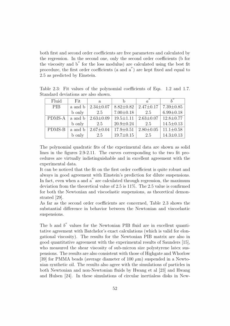
2.12 Intrinsic steady shear viscosity (top) and intrinsic loss modulus(bottom) for the three suspensions as function of volume fraction 54

2.13 The percent error for three different frequencies (0.1, 1 and 10rad/s), for both the calculation of G

′() and G

′′(5) . . . . . . 55

2.14 The ratio of the loss over the storage modulus versus frequencyfor filled and unfilled PDMS fluids. . . . . . . . . . . . . . . . 56

2.15 Comparison between normalized viscous modulus for PDMSbased suspensions in the low frequency range and in the wholefrequency range. Line is the best fit to data. . . . . . . . . . . 58

2.16 Relative storage modulus as function of volume fraction forthe suspending media. The lines are best fits to the data. . . . 59

2.17 Comparison between data of viscous modulus for PDMS-Bbased suspensions at 70C with those at 30C. . . . . . . . . . 61

2.18 DFST for pure suspending atactic polypropylene . . . . . . . . 622.19 Loss (a) and storage (b) moduli for a-PP based suspensions

as function of frequency at various filler concentrations. . . . . 632.20 Normalized viscous modulus for the a-PP suspension as func-

tion of bead volume fraction. . . . . . . . . . . . . . . . . . . . 642.21 Normalized storage modulus for the a-PP suspension as func-

tion of bead volume fraction. . . . . . . . . . . . . . . . . . . . 642.22 N1 as function of shear rates for different volume fractions.

Symbols as in Fig. 2.20. . . . . . . . . . . . . . . . . . . . . . 652.23 Normalized value of N1 as function of volume fraction. . . . . 66

7

2.24 Normalized viscous modulus as function of the longest relax-ation time λmax for the three suspending media, for differentvolume fractions. . . . . . . . . . . . . . . . . . . . . . . . . . 68

3.1 The geometry used in the simulation technique. . . . . . . . . 733.2 The angular velocity as function of ωt. . . . . . . . . . . . . . 753.3 Fluid (top) and particle (bottom) contributions to the shear

bulk stress as function of particle size. . . . . . . . . . . . . . 763.4 Viscous modulus as function of solid area fraction. The line is

the best fit to the data. . . . . . . . . . . . . . . . . . . . . . . 763.5 The division of the domain box in four sub-domains; one par-

ticle is in the center of the box; the initial position of the otherparticle is changed. . . . . . . . . . . . . . . . . . . . . . . . . 77

3.6 The viscous modulus as function of solid area fraction. Thedashed line is Einstein’s result for 2-D flow [26]. The solid lineis a quadratic regression to the data. . . . . . . . . . . . . . . 78

4.1 SEM micrographs of Polystyrene spheres. From the top to thebottom, 2.8 µm, 1.9 µm and 1.2 µm respectively. . . . . . . . 82

4.2 Schematic diagram of SALS setup . . . . . . . . . . . . . . . . 844.3 Schematic layout of a SALS setup dipicting the incident and

scattered beams, the 2-D detector and the definition of thescattered vector (q). . . . . . . . . . . . . . . . . . . . . . . . 85

4.4 Real space image of a flow aligned structure and the corre-sponding image in the SALS pattern (respectively top left andtop right). Scattering pattern before shearing and after shear-ing for PS suspensions in HPC. . . . . . . . . . . . . . . . . . 87

4.5 The counterrotating rheometer combined with microscopy from[55]. . . . . . . . . . . . . . . . . . . . . . . . . . . . . . . . . 89

4.6 Viscosity of the fluids as function of shear rate. . . . . . . . . 904.7 First normal stress coefficients of the fluids as function of shear

rate. . . . . . . . . . . . . . . . . . . . . . . . . . . . . . . . . 904.8 Weissenberg numbers of the fluids as function of shear rate. . . 914.9 Viscoelastic moduli for the suspending media as function of

frequency. . . . . . . . . . . . . . . . . . . . . . . . . . . . . . 924.10 Microscopy image of PEO’s suspension with 3µm diameter

spheres. . . . . . . . . . . . . . . . . . . . . . . . . . . . . . . 924.11 Microscopy images of a HPC suspension at 30s−1 and 200µm

gap (diameter spheres=1.9 µm). After 1h: on the left side themicrostructure on the plate; on the right side in the bulk. . . . 94

8

4.12 Microscopy image of a HPC suspension at 30s−1, 100µm gap(diameter spheres=3µm). Top left: before shearing. Topright: on the plate after shearing 1h. Bottom: in the bulkafter shearing 1h. . . . . . . . . . . . . . . . . . . . . . . . . . 94

4.13 Microscopy image of a HPC suspension at different shear rates(diameter spheres: 1.9µm) after shearing 1h at 100µm gap. . . 95

4.14 Microscopic image of HPC suspension with 1.2µm spheres inthe bulk of the liquid after shearing at 1 s−1. . . . . . . . . . . 96

4.15 The sign evaluation of cos2ϑ for the alignment factor. . . . . . 974.16 Evaluation of percent error in a meaningful q range for 1.9 µm

based suspension. . . . . . . . . . . . . . . . . . . . . . . . . . 984.17 SALS patterns as function of shear rate for 1.2 µm size par-

ticle. At low shear rates, a weak vorticity alignment can besee. Increasing the shear rate reorients the strings in the flowdirection. . . . . . . . . . . . . . . . . . . . . . . . . . . . . . 98

4.18 Alignment factor as function of scattering vector at 360%strain for the 1.2 µm size suspension. . . . . . . . . . . . . . . 99

4.19 Alignment factor as function of scattering vector after 1h for1.2 µm size spheres. . . . . . . . . . . . . . . . . . . . . . . . . 100

4.20 Alignment factor as function of shear rate at a scattering vec-tor of 1µm−1. . . . . . . . . . . . . . . . . . . . . . . . . . . . 100

4.21 Alignment factor (eq. 4.6) as function of scattering vector forthe suspensions with 1.2µm particles at different shear ratesafter 1h of shearing. . . . . . . . . . . . . . . . . . . . . . . . . 101

4.22 Alignment factor at steady state as function of shear rate forsuspensions with spheres of different sizes. Data for suspen-sions with 2.8µm spheres are from Scirocco et al [91]. . . . . . 102

4.23 Effect of the gap width on the alignment factor for a disper-sion of 1.9µm spheres in the HPC based suspending medium.Steady state at q=1µm−1. . . . . . . . . . . . . . . . . . . . . 103

4.24 Alignment factor as function of the time for different gap sizes. 1044.25 First derivative of the alignment factor in fig. 4.23 in the range

0-600s. . . . . . . . . . . . . . . . . . . . . . . . . . . . . . . . 1044.26 Alignment factor as function of time for a gap of 100µm at

30s−1. . . . . . . . . . . . . . . . . . . . . . . . . . . . . . . . 1054.27 Bands of particles at high shear rates. . . . . . . . . . . . . . . 1054.28 SALS patterns as function of shear rate for 1.6 µm size charged

particle. . . . . . . . . . . . . . . . . . . . . . . . . . . . . . . 1064.29 Counterrotating image for HPC based suspensions. . . . . . . 1084.30 Alignment factor as defined by eq. 4.7 at steady state as func-

tion of shear rate for suspensions of spheres with different sizes.109

9

List of Tables

2.1 Zero shear viscosities of the suspending fluids . . . . . . . . . 382.2 Comparison between required and effective volume fractions . 412.3 Fit values of the polynomial coefficients of Eqs. 1.2 and 1.7.

Standard deviations are also shown. . . . . . . . . . . . . . . . 522.4 Best fit values for b

′of eq. 1.8 and comparison with b

′′of

eq. 1.7 with the assumption that a′

= a′′

= 2.5. Standarddeviations are also reported to appreciate the statistical error. 60

2.5 Parameters of eq. 1.7 and 1.8 for PDMS-B based suspensionsat 30C and 70C. . . . . . . . . . . . . . . . . . . . . . . . . 60

2.6 Longest relaxation time λmax for the suspending media. . . . . 68

4.1 Molecular weights of the polymers and composition of the sus-pending media. . . . . . . . . . . . . . . . . . . . . . . . . . . 83

4.2 Weissenberg number and onset of alignment as function ofshear rate. . . . . . . . . . . . . . . . . . . . . . . . . . . . . . 96

10

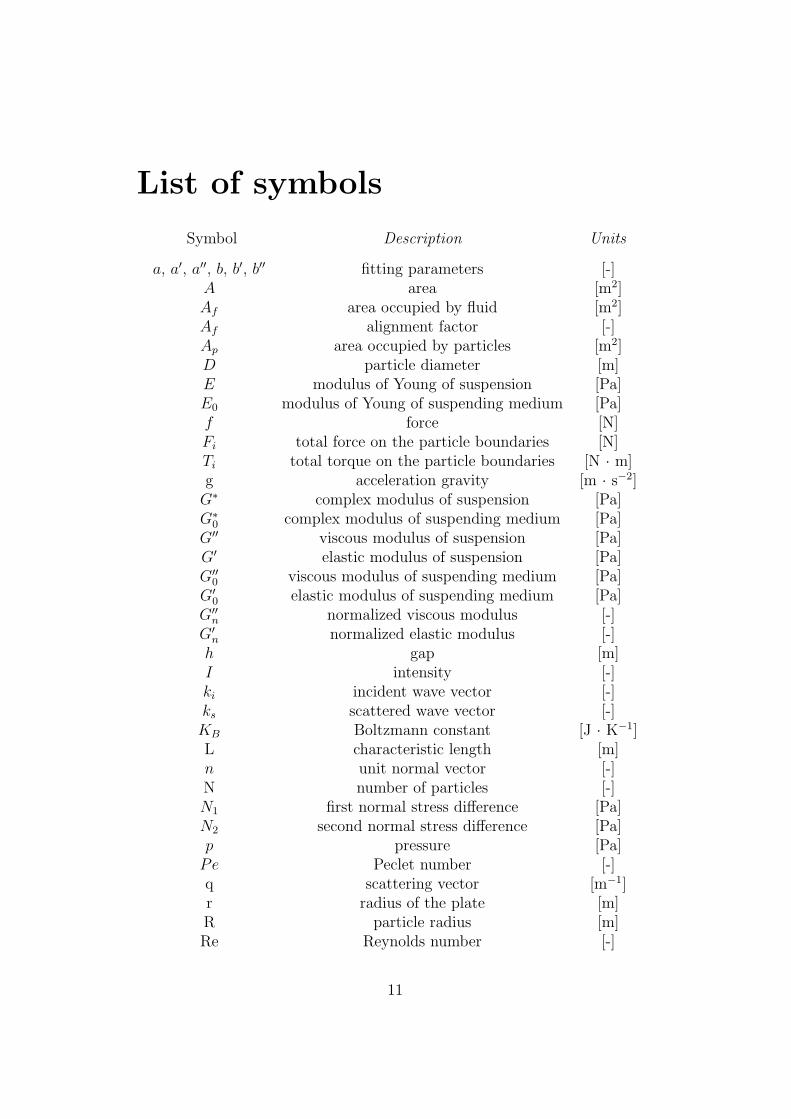
List of symbols

Symbol Description Units

a, a′, a′′, b, b′, b′′ fitting parameters [-]A area [m2]Af area occupied by fluid [m2]Af alignment factor [-]Ap area occupied by particles [m2]D particle diameter [m]E modulus of Young of suspension [Pa]E0 modulus of Young of suspending medium [Pa]f force [N]Fi total force on the particle boundaries [N]Ti total torque on the particle boundaries [N · m]g acceleration gravity [m · s−2]

G∗ complex modulus of suspension [Pa]G∗

0 complex modulus of suspending medium [Pa]G′′ viscous modulus of suspension [Pa]G′ elastic modulus of suspension [Pa]G′′

0 viscous modulus of suspending medium [Pa]G′

0 elastic modulus of suspending medium [Pa]G′′

n normalized viscous modulus [-]G′

n normalized elastic modulus [-]h gap [m]I intensity [-]ki incident wave vector [-]ks scattered wave vector [-]KB Boltzmann constant [J · K−1]L characteristic length [m]n unit normal vector [-]N number of particles [-]N1 first normal stress difference [Pa]N2 second normal stress difference [Pa]p pressure [Pa]

Pe Peclet number [-]q scattering vector [m−1]r radius of the plate [m]R particle radius [m]Re Reynolds number [-]

11

Rep particle Reynolds number [-]s spacing between two spheres [m]T temperature [K]t time [s]u velocity vector [m · s−1]

Ui, Vi components of the translational velocity [m · s−1]vz migration velocity [m · s−1]w angular velocity [s−1]

Wi Weissenberg number [-]Wicr critical Weissenberg number [-]Xi, Yi coordinates of the particle center [-]x, y, z coordinates [-]

Greek symbols

α polar angle [-]γ deformation [-]γ0 amplitude of deformation [-]δ ratio between G′′ and G′ [-]γ shear rate [s−1]λ wavelength of the light [m]

λmax maximum relaxation time [s]η0 viscosity of suspending medium [Pa · s]η viscosity of suspension [Pa · s]ηn normalized viscosity [-]θ azimuthal angle [-]σ shear stress [Pa]ρ0 density of suspending medium [Kg · m−3]ρp particle density [Kg · m−3]φ volume fraction [-]φa area fraction [-]φm volume fraction at maximum packing [-]ψ1 first normal stress coefficient [Pa · s−2]ω frequency [s−1]Ω bounded region [s−1]

12

Contents

0.1 Introduction . . . . . . . . . . . . . . . . . . . . . . . . . . . . 15

1 State of the art 181.1 Rheological properties of suspensions . . . . . . . . . . . . . . 18

1.1.1 Viscosity of suspensions of spheres in Newtonian media 181.1.2 Viscosity and viscoelastic properties for suspensions of

spheres in non-Newtonian Media . . . . . . . . . . . . 261.2 Hydrodynamics and interaction forces . . . . . . . . . . . . . . 31

1.2.1 Newtonian media . . . . . . . . . . . . . . . . . . . . . 311.2.2 Non-Newtonian media . . . . . . . . . . . . . . . . . . 32

2 Suspension Rheology 382.1 Materials and Methods . . . . . . . . . . . . . . . . . . . . . . 38

2.1.1 Materials . . . . . . . . . . . . . . . . . . . . . . . . . 382.1.2 Preparation of the suspensions . . . . . . . . . . . . . . 402.1.3 Rheological measurements . . . . . . . . . . . . . . . . 42

2.2 Experimental results-A . . . . . . . . . . . . . . . . . . . . . . 442.2.1 Rheology of suspending fluids . . . . . . . . . . . . . . 442.2.2 Rheology of suspensions . . . . . . . . . . . . . . . . . 45

2.3 Experimental results-B . . . . . . . . . . . . . . . . . . . . . . 622.3.1 Rheology of atactic-polypropylene . . . . . . . . . . . . 622.3.2 Rheology of the suspensions . . . . . . . . . . . . . . . 62

2.4 Conclusions . . . . . . . . . . . . . . . . . . . . . . . . . . . . 67

3 Simulation of circular disks in a Newtonian fluid under 2-Doscillatory flow 693.1 Modeling aspects . . . . . . . . . . . . . . . . . . . . . . . . . 703.2 Bulk stress . . . . . . . . . . . . . . . . . . . . . . . . . . . . . 733.3 The single particle problem . . . . . . . . . . . . . . . . . . . 743.4 The two particles problem . . . . . . . . . . . . . . . . . . . . 773.5 Conclusions . . . . . . . . . . . . . . . . . . . . . . . . . . . . 79

13

4 Flow-induced structure formation of spheres in viscoelasticfluids 804.1 Materials . . . . . . . . . . . . . . . . . . . . . . . . . . . . . 80

4.1.1 Polystyrene particles . . . . . . . . . . . . . . . . . . . 804.1.2 Polymer solutions . . . . . . . . . . . . . . . . . . . . . 82

4.2 Experimental techniques . . . . . . . . . . . . . . . . . . . . . 834.3 Experimental results . . . . . . . . . . . . . . . . . . . . . . . 90

4.3.1 Rheology of suspending fluids . . . . . . . . . . . . . . 904.3.2 Microscopy . . . . . . . . . . . . . . . . . . . . . . . . 924.3.3 Small angle light scattering . . . . . . . . . . . . . . . 974.3.4 Counterrotating device . . . . . . . . . . . . . . . . . . 107

4.4 Conclusions . . . . . . . . . . . . . . . . . . . . . . . . . . . . 108

14

0.1 Introduction

Rheology is the science that studies the deformation and flow of matter.It is a relatively young and multidisciplinary science that encompasses manydifferent industrial areas of activity as plastics, ceramics, cosmetics, pharma-ceutics, food and biotechnology, but also paints and inks, adhesives, lubri-cants and surfactants.It is quite straightforward to list situations where the deformation or the flowof matter (which depends on the rheological characteristics of the involvedmaterials) determines the performance of a product, the effectiveness of aservice and the rate of a manufacturing process. Thus, rheology is a very at-tractive, dynamic, highly multidisciplinary and fast-growing area of activity.In particular, in many industrial processes, materials consist of particles dis-persed in rheologically complex fluids, the so called suspensions.

Suspensions of particles find applications in many different areas, includingpolymers, pharmaceuticals, cosmetics, food, ceramic pastes. The control ofstructure and flow properties of suspensions is often crucial to the commercialsuccess of the product. The final properties of suspensions are affected byseveral factors, including shape, concentration and size of the filler. In par-ticular, the size of solid inclusions can range from nanoscopic to macroscopiccharacteristic dimensions, leading to a wide range of different flow behaviors.

The rheological behavior of suspensions has received considerable attention inthe literature. Most studies have focused on highly filled systems (typically,volume fractions greater than 10%), due to their importance in technologicalapplications. Conversely, relatively few studies are done on the rheology of di-lute or semi-dilute suspensions. Low concentrations are important, however,at least for two reasons: first, low concentration suspensions find applicationsin several fields (biomedical materials, cosmetics). Second, the experimentalresponse of semi-dilute suspensions is a good test for theories that exploreconcentrations beyond the well known Einsteins infinite dilution result.

It must be added that most investigations in the low concentration range werecarried out on particles suspended in a Newtonian liquid. Indeed, dispersingparticles will be different depending on whether the suspending medium isNewtonian or non-Newtonian. Viscoelastic fluids, in particular, exhibit shearthinning, memory effects and first and second normal stress differences, assuch increasing the rheological complexity of the whole system.Compared to the Newtonian suspensions, suspensions with viscoelastic sus-pending media show differences in the flow induced structure.

15

The macroscopic response and the flow induced microstructure depend onthe dynamics of the individual particles and the flow of the suspendingfluid around and between the particles. The differences between Newtonianand viscoelastic suspensions are mainly due to the changes in hydrodynamicforces that are associated to the changes in the rheological behavior of thesuspending fluids. Phenomena of chaining and alignment can occur in vis-coelastic suspending media and there is no indication that this also happensin Newtonian media.

In order to understand the formation of such microstructures, one needs tofully consider the hydrodynamic interactions between particles and fluid, theinter-particle forces as well as the complex rheological properties of the fluid.To accommodate all these requests, the development of simulation methodshas received great attention in recent years. In particular, direct numericalsimulation techniques give sufficiently accurate results on velocity and stressfields in the fluid medium, along with full consideration of hydrodynamic andinterparticular interactions with the usage of state-of-the-art viscoelastic con-stitutive models. To our knowledge, most investigations have been carriedout on direct numerical simulations for inertialess non-Brownian hard parti-cle suspensions, with Newtonian and viscoelastic fluids, in both simple shearand elongational two-dimensional flows.

Objectives

The main objective of this study is to elucitade the role and effect of theviscoelasticity of the dispersion medium on the rheology and microstructureof dilute suspensions of spherical particles.In particular, the dependence of viscoelastic moduli and shear viscosity onvolume fraction and frequency has been experimentally studied for differentparticle-polymer systems.Moreover, a new simulation technique for non-Brownian inertialess hardsphere suspensions in oscillatory flow for a Newtonian fluid will be presented,in order to understand how the complex viscosity changes as a function ofsolid area fraction (two-dimensional flow).The microstructure generated in flowing suspensions has been also consid-ered. The knowledge of this study provides the basis for understanding theprocessing of suspensions as well as predicting and controlling the final prop-erties of the processed products.

16

Approach

The macroscopic rheology of several non-colloidal, inertialess rigid spheres inboth Newtonian and viscoelastic fluids is investigated. Volume fractions upto 10% were used, thus exploring both the dilute regime, which is commonlydelimited to a concentration of about 5% [1], and the semi-dilute regime,where interparticle interactions are expected to become relevant. The ex-perimental results are compared with the predictions of existing theories, inparticular those based on purely hydrodynamic calculations.

In addition, suspensions of monodisperse polystyrene spheres in differentsuspending media have been studied. The goal is to use microscopy andscattering techniques to understand how particle dynamics are altered andhow the overall suspension rheology is affected in a viscoelastic fluid. Theeffect of the size of the spheres on flow-induced alignment has been consid-ered. Walls effects and migration have been considered.

This thesis is organized as follows: in chapter 1 the state of the art is re-viewed. This chapter covers the rheology of suspensions of spheres in bothNewtonian and viscoelastic suspending media, with particular attention tothe theoretical models and experimental background, and also focuses on themotion and suspension microstructure.The experimental results are divided in three sections. In the first sectionresults on the macroscopic rheological response for a Newtonian and someviscoelastic suspensions are presented. The behavior of model suspensionscomposed of non Brownian, inertialess, rigid spheres immersed in Newtonianand viscoelastic matrices is investigated in the range of volumetric concentra-tions up to 10%, thus encompassing both the dilute and semidilute regimes.The data are modeled by means of quadratic polynomial functions of theparticle volume fraction in order to make a comparison with theoretical, em-pirical and experimental models.The second section reports on a new simulation technique for suspensions inNewtonian fluid with imposed oscillatory flow. The case of a single sphereand of two interacting spheres are studied and fully discussed.The last section focuses on flow-induced alignment of non-colloidal particlesin viscoelastic fluids. The phenomenon is treated systematically in order toquantify the alignment of particles and try to correlate it with the rheology ofthe fluid, the size of the suspending particles, the interactions with the wall.For the first and last section, materials and used methods are presented andobtained results are discussed.

17

Chapter 1

State of the art

In many industrial processes, materials are formulated that consist of parti-cles dispersed in rheologically complex fluids. In order to control the process-ing behavior and to tune the end-use properties of formulated products, astudy of the rheological properties and generated microstructure is necessary.In this first chapter the state of the art, pertaining to the subject of this the-sis, is presented. In particular, the first section focuses on the macroscopicresponse of suspensions: the suspension rheology. Major contributions, the-oretical, experimental and from computer simulation are discussed. BothNewtonian and non-Newtonian suspending media are covered.The second part of this chapter deals with particle motion and flow inducedmicrostructure in suspensions in shear flow.

1.1 Rheological properties of suspensions

1.1.1 Viscosity of suspensions of spheres in Newtonianmedia

Viscosity is the most fundamental rheological property in characterizing thestructural organization and interaction of constituents within suspensions.The simplest model suspension is composed of so-called hard spheres in aNewtonian fluid. The addition of a rigid sphere to a liquid alters the flowfield, and this influence has been the subject of a vast literature.If spheres are very small (<1 micron), colloidal forces between particles canbecome enormous and can also introduce deviations from Newtonian behav-ior.For the case of rigid spheres in a Newtonian fluid at very low concentra-

18

tion hydrodynamic effects were accounted by Einstein [2] 100 years ago. Hegave the first prediction for the viscosity of dilute suspensions. The relevantassumptions for the analysis in Einstein’s classic paper are the following:

• The surrounding fluid or solvent is incompressible and Newtonian andcan be treated as a continuum. This implies that the fluid moleculesare much smaller than the suspended particles.

• Creeping, buoyancy-free flow.

• No slip between particles and fluid.

• Particles are rigid and spherical.

• Dilute non-interacting particles are considered.

• The viscometer characteristic length is much greater than that of thesuspended particles, so that wall effects neglectable.

All these assumptions lead to Einstein’s celebrated formula:

η = η0(1 + 2.5φ) (1.1)

with η the viscosity of the suspension, η0 the viscosity of the suspending fluidand φ the volume fraction of spheres.The experimental confirmation of eq. (1.1) is not so trivial, as the assump-tions of Einstein’s theory are not easily satisfied. Reports on experimentscan be found in literature, especially in the 30’s, for example by Bachle [3],Blow [4], Eirich et al [1]. In the latter work spherical particles were used andthe total absence of agglomeration was observed. Under these conditions,the equation (1.1) was verified up to volume concentrations of 5%.For more concentrated suspensions it is necessary to consider corrections tothe viscosity that are of higher order in the volume fraction. When the flowfield around a sphere is influenced by the presence of neighbouring spheres,the hydrodynamic interactions cannot be neglected and they could be treatedas a contribution to η that is proportional to φ2 for two bodies, to φ3 for threebodies and so on.The major contribution to theory comes from Batchelor and Green [5, 6] andBatchelor [7], who performed a fully hydrodynamic calculation using statisti-cal mechanics to account for Brownian forces and hydrodynamic interactionsin a semidilute suspension of hard spheres. Interactions between particlesdetermine the presence of terms of order φ2 in the expression for the stresstensor. In particular, it was assumed that [6]:

19

• The fluid is Newtonian.

• Creeping flow is assumed.

• Inertia of the particles can be neglected.

• No external forces or couples act on the particles.

• The particles are spherical and their spatial distribution throughoutthe ambient fluid is assumed to be random.

With these assumptions, the suspension has isotropic structure and the stressbehaviour can be represented to order φ2 in terms of an effective viscosity:

η = η0(1 + aφ + bφ2) (1.2)

In eq. (1.2), obviously, a=2.5. The second order coefficient b is equal to 7.6[6]. It becomes equal to 6.2 [7] when Brownian motion is included.It must be stressed that Batchelor’s result is a prediction for purely irro-tational flow only, where the particle probability function can be exactlycalculated. As a consequence, eq. (1.2) is a prediction for an elongationalviscosity, not for a shear viscosity. Exact predictions for the shear viscosityof interacting particles have never been developed. Extensions to the workof Batchelor to higher volume fractions always contained several, arbitraryassumptions [8].Experimental validations of Batchelor’s calculations (assuming that the pre-diction of (1.2) holds also for shear flow) are very scarce in the literature. Amajor review of the dependence of the relative viscosity on concentration isdue to Rutgers [9], who collected the results of several experimental inves-tigations up to very high concentrations [9, 10, 11, 12, 13, 14]. From thesemeasurements on suspensions of spheres in Newtonian fluids, he found anaverage curve which represents a new relation valid for all shear rates up toa volume fractions of about 0.25. Fig. (1.1) presents the relative viscosity ηn

(the ratio between the viscosity of suspensions and that of pure suspendingmedium) vs the volume fraction φ and also the average curve obtained byRutgers, whose results are presented in the accompanying table.

20

Figure 1.1: Data from Rutgers.

From all the investigations on Newtonian suspensions shown in Fig. 1.1, theonly relevant contribution for low concentrations is that of Saunders [15], whomeasured the shear viscosity of sub-micron sized polystyrene lattice suspen-sions and found that a good agreement with Batchelor’s equation for volume

21

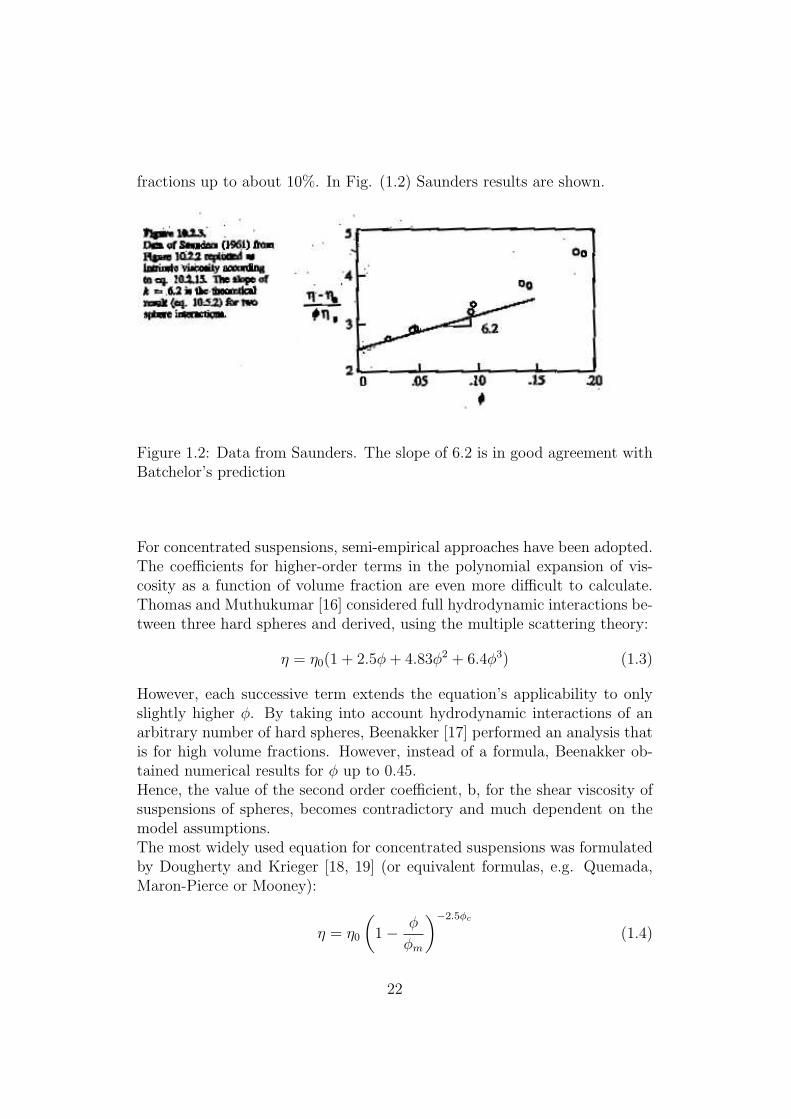
fractions up to about 10%. In Fig. (1.2) Saunders results are shown.

Figure 1.2: Data from Saunders. The slope of 6.2 is in good agreement withBatchelor’s prediction

For concentrated suspensions, semi-empirical approaches have been adopted.The coefficients for higher-order terms in the polynomial expansion of vis-cosity as a function of volume fraction are even more difficult to calculate.Thomas and Muthukumar [16] considered full hydrodynamic interactions be-tween three hard spheres and derived, using the multiple scattering theory:

η = η0(1 + 2.5φ + 4.83φ2 + 6.4φ3) (1.3)

However, each successive term extends the equation’s applicability to onlyslightly higher φ. By taking into account hydrodynamic interactions of anarbitrary number of hard spheres, Beenakker [17] performed an analysis thatis for high volume fractions. However, instead of a formula, Beenakker ob-tained numerical results for φ up to 0.45.Hence, the value of the second order coefficient, b, for the shear viscosity ofsuspensions of spheres, becomes contradictory and much dependent on themodel assumptions.The most widely used equation for concentrated suspensions was formulatedby Dougherty and Krieger [18, 19] (or equivalent formulas, e.g. Quemada,Maron-Pierce or Mooney):

η = η0

(1− φ

φm

)−2.5φc

(1.4)

22

where φm is an adjustable parameter related to the volume fraction at whichspheres become close packed. Typical values for φm range from 0.6 to 0.7for monodisperse spheres. The -2.5 used in the exponent is used in order tore-obtain the Einstein’s solution when φ → 0.Another model to be mentioned for the effective viscosity of Newtonian sus-pensions of monosized spheres is the one derived by Hsueh and Becher [20].The derived formula is in a good agreement with Beenakker’s numerical sim-ulation. In particular, the power series expansion of the viscosity equationreported in this work is:

η = η0(1 + 2.5φ + 6.25φ2 + 10φ3 + 13.75φ4 + 17.5φ5 + 21.25φ6 + ...) (1.5)

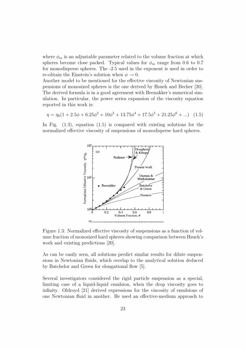
In Fig. (1.3), equation (1.5) is compared with existing solutions for thenormalized effective viscosity of suspensions of monodisperse hard spheres.

Figure 1.3: Normalized effective viscosity of suspensions as a function of vol-ume fraction of monosized hard spheres showing comparison between Hsueh’swork and existing predictions [20].

As can be easily seen, all solutions predict similar results for dilute suspen-sions in Newtonian fluids, which overlap to the analytical solution deducedby Batchelor and Green for elongational flow [5].

Several investigators considered the rigid particle suspension as a special,limiting case of a liquid-liquid emulsion, when the drop viscosity goes toinfinity. Oldroyd [21] derived expressions for the viscosity of emulsions ofone Newtonian fluid in another. He used an effective-medium approach to

23

relax the hypothesis of diluteness. Oldroyd’s prediction for the coefficientb in (1.2) was b=2.5, far smaller than Batchelor’s exact calculation. Alongsimilar lines Choi and Schowalter [22], using a cell model approach, obtainedthe prediction b=125/8, an amazingly different result.

A new approach for the study of suspensions is Computational Fluid Dy-namics. Its current popularity is rooted in the perception that informationimplicit in the equations of fluid motion can be extracted without approxi-mation using direct numerical simulation.Numerical simulations of fluidsolid flow systems can be classified in differentcategories, as it will be explained later.For our purpose, in particular, two articles from Hwang et al [23, 24] and onefrom D’Avino et al [25] on simulations of circular inertialess disks in a New-tonian fluid have to be mentioned. In their articles, only two-dimensionalsimple shear and two-dimensional planar elongational flows are simulated.In the case of simple shear flow, Hwang et al calculated the bulk shear viscos-ity as function of solid area fraction for a wide range of the area fraction, fromless than 1% to about 75%. The bulk shear viscosity is plotted as functionof φ in Fig. 1.4.

Figure 1.4: Time-averaged bulk shear viscosity as a function of solid areafraction, calculated from the single particle problem [23].

As regards elongational flow, the relative bulk viscosity as a function of theparticle area fraction was obtained as in Fig. 1.5.

24

Figure 1.5: Relative bulk shear viscosity as a function of solid area fraction.Hwang and Hulsen results [24] are plotted as well (open squares).

To clarify Fig.(1.4) and 1.5, it has to be stressed that Einstein’s classicalresult for a dilute suspension with circular disk particles is given by [26]:

η = η0(1 + 2φ) (1.6)

as opposed to the factor 2.5 in three-dimensional flow.In the dilute concentration limit, Fig. (1.4) and 1.5 show that Einstein’sresult is recovered. A clear deviation from Einstein’s result appears at volumefraction of about 5%. For a volume concentration of 10% there is an increasein the viscosity of about 4% which means a second order factor in the Eq.(1.2)equal to 4.

25

1.1.2 Viscosity and viscoelastic properties for suspen-sions of spheres in non-Newtonian Media

If both theoretical and experimental studies for dilute and semi-dilute sus-pensions in Newtonian matrices are relatively scarce and somewhat contra-dictory, the situation is even worse for suspensions in viscoelastic fluids. Therheology of suspensions in non Newtonian media is, from a technologicalpoint of view, more important than its counterpart in Newtonian media. Im-portant industrial applications are the processing of filled polymers, technicalceramic pastes and drilling muds for oil recovery. In particular, in the last fewdecades the emergence of filled plastics and composites as high-performanceand cost effective materials has attracted considerable attention towards therheology of polymer suspensions.Typically, viscoelastic fluids exhibit a shear thinning viscosity, first and sec-ond normal stress differences, and memory effects. Suspending solid particlesin these fluids leads to an even more complex flow behavior.Theoretical analysis of suspensions in non-Newtonian media are only avail-able for high volume fractions [27], where lubrication hydrodynamics domi-nate the interactions (and only for the viscosity function).Koch et al. [28] provide the first reliable theoretical prediction for the stressin a three-dimensional suspension of spherical particles in a viscoelastic fluid.Unfortunately, the result is restricted to a homogeneous, dilute suspension(to order φ) and linear velocity field.It’s possible [29, 30, 31, 32], however, following Einstein’s and Batchelor’sapproaches, to express the fluid viscoelastic properties in terms of a seriesexpansion in the solid volume fraction, that is:

G′′

= G′′0

(1 + a

′′φ + b

′′φ2

)(1.7)

G′ = G′0

(1 + a′φ + b′φ2

)(1.8)

Palierne [33, 29] exactly calculated the first order coefficients a′

and a′′

ofEq. (1.7)-(1.8) via direct hydrodynamic calculations. He was able to showthat a′ = a

′′= 2.5.

There are no exact calculations for the second order coefficient. However,some empirical models have been proposed. Palierne [29], using a cell modelapproach for emulsions and blends, obtained the following prediction for thelimiting case of non Brownian rigid spheres in a viscoelastic medium:

G∗ = G∗0

(1 + 1.5φ

1− φ

)(1.9)

26

where G∗ is the complex modulus of the suspension and G∗0 that of the matrix

fluid. When expanded into power series, Eq. (1.9) gives the first order resultcorrectly whereas it predicts b

′= b

′′= 2.5 for the quadratic coefficient.

Based on the work of Palierne [29], three different viscoelastic empirical mod-els for suspensions at any concentration were developed using also the max-imum packing volume fraction, φm as parameter. The model predictions forthe viscoelastic properties are complex. When expanded in power series ofthe volume fraction, the three models yield:

G∗ = G∗0

(1 + 2.5φ + 4.4φ2

)(1.10)

G∗ = G∗0

(1 + 2.5φ + 7φ2

)(1.11)

G∗ = G∗0

(1 + 2.5φ + 5.1φ2

)(1.12)

where the value φm=0.64 has been used.It should be noted that, like the purely Newtonian models for the viscosity,the viscoelastic models presented above show contradictory predictions forthe second order coefficient. They share, however, the common feature thatG′and G

′′have the same dependence upon the solid volume fraction.

Guth [31, 32] introduced a new quadratic term to explain the reinforcingeffect of elastomers and found the following equations for the viscosity andmodulus of Young E:

η = η0

(1 + 2.5φ + 14.1φ2

)(1.13)

E = E0

(1 + 2.5φ + 14.1φ2

)(1.14)

valid with concentrations up to 10% of spherical particles.Guth’s work deals with a ”solid” suspending medium, it can however stilluseful to understand that changing the properties of the suspending mediumcould bring about a change (and, specifically, an increase) in the quadraticterm of polynomial functions both for viscosity and viscoelastic moduli.Elucidating a quantitative value for the quadratic term of the polynomial isone of the major objectives of this work.

Concerning the study of normal stress differences, the work by Koch et al[28] gives the first theoretical result on the first normal stress difference for adilute (at order φ) suspension of spherical particles in a viscoelastic fluid. At

27

a given shear rate the first normal stress difference is increased by the samefactor, 1+2.5φ, as the shear stress. The second normal stress difference, in-stead, is increased by a larger factor.The first normal stress difference, N1, has been experimentally characterizedfor various viscoelastic suspensions. The first normal stress difference is pos-itive but usually decreases with filler amount when compared at constantshear stress [34, 35]. The second normal stress difference of viscoelastic sus-pensions has been recently investigated for solid fraction up to 0.25 [34]. Incontrast to N1, N2 is negative with a magnitude that increases with volumefraction of the filler. The variations of the first and second normal stress dif-ferences are represented by power law functions of the imposed shear stresswith an exponent that appears to depend on the specific matrix fluid usedin preparing the suspensions and independent of the particle volume fraction[36].

Concerning numerical simulations, there are some interesting calculationson the relative shear viscosity as function of solid area fraction in two-dimensional flow for viscoelastic suspensions:

Figure 1.6: Relative shear viscosity as a function of solid area fraction fordifferent Weissenberg numbers [37].

28

As shown in Fig.(1.6), the bulk shear viscosity increases with the Weissenbergnumber as well as with the solid area fraction. The Weissenberg number is ameasure for the degree of viscoelastic behavior and is a dimensionless number,defined as the ratio of the first normal stress difference over the shear stressat a certain rate:

Wi =N1

σ(1.15)

The higher the Weissenberg number, the more elastic the fluid; the lower theWeissenberg number the more Newtonian the fluid. For small values of φ, theshear viscosity of the viscoelastic system converges to Einstein’s analyticalresult for a dilute suspension in a Newtonian fluid (Fig.1.6) [26]. However,limited information about the comparable three-dimensional flow for one ortwo particles was presented.To our knowledge, no simulations are performed in order to check the depen-dence of the viscoelastic moduli on volume fraction.

Many experimental results on the rheology of viscoelastic suspensions canbe found in the literature.In the case of filled polymeric systems, Kitano et al [38] proposed that the dy-namic data may be reduced relative to the data of the matrix polymer at thesame frequency, in the hope that the relative properties would be functionsof the volume fractions of particulates and their properties but independentof the frequency. Kitano et al showed that these functions for compositesystems filled with glass fibers are dependent on the volume fractions andthe frequency.Highgate and Whorlow [39] measured the steady shear viscosity of PMMAbeads suspended in several fluids, for volume concentrations up to 10%. Theyfocused, however, on the flow curve behavior and did not systematically studythe zero-shear rate concentration dependence.In general the literature focuses on high solid concentrations (typically above10%)and this is beyond the scope of the present work.

Faulkner and Schmidt [40] studied polypropylenes filled with glass beads forconcentrations up to about 30%. They found that the relative loss modulusgrows with the square of volume fraction and the relative storage modu-lus (moduli of filled material normalized with respect to the moduli of purepolymer) grows linearly with volume fraction as follows.

G′n = 1 + 1.8φ (1.16)

G′′n = 1 + 2φ + 3.3φ2 (1.17)

29

The calculation of these polynomial functions was made at a fixed frequencyand for a wide range of volume fractions up to about 30%. This means thatthe ratio G

′′n/G

′n should be a decreasing function of volume fraction. No dis-

cussion is provided for the choice of the frequency.Poslinsky et al. [41] studied thermoplastics filled with glass beads for con-centrations up to 60% and found that the relative loss modulus grows morethan linearly with the filler volume fraction. See et al. [42] studied Separanpolymer solutions filled with PE particles for concentrations up to 40% andfound in contrast to Faulkner and Schimdt [40], that the relative storage andloss moduli follow similar scaling. They also reported an equation for therelative elastic modulus:

G′n = [1 +

φ

φm

]−2 (1.18)

where φm is the maximum packing volume fraction. Aral and Kalyon [43]studied dynamic properties, relaxation modulus and first normal stress dif-ference for a polydimethylsiloxane matrix loaded with glass beads for con-centrations up to 60%. They found that the increase of solid concentrationincreases the elasticity.Walberer and McHugh [44] studied the frequency moduli of glass bead filledpolydimethyl siloxanes (PDMS). They examined the influence of molecularweight on the ratio G

′′/G

′frequency and volume fraction and found that,

as the molecular weight increases, the difference between G′′/G

′of unfilled

and filled materials at low frequencies is progressively smaller until it nearlydisappears for the highest molecular weights.Le Meins et al [45] reported experimental results on suspensions of monodis-perse spheres dispersed in a liquid polymer for volume concentrations upto 31%. The measurements included steady-state viscosity, dynamic moduliand non linear stress relaxation. They found that in the hydrodynamic limit,particles increases in the same way both storage and loss moduli and similarto the Newtonian steady viscosity.

30

1.2 Hydrodynamics and interaction forces

1.2.1 Newtonian media

Rotation, interactions and migration of particlesThe motion of isolated particles suspended in Newtonian fluids is well under-stood. Particles rotate with a rate equal to half the shear rate and translatewith the local velocity of the fluid. An important conclusion is that the rota-tion speed of the particle is independent of a particle radius and the viscosityof the fluid.When moving to higher volume fractions, instead, hydrodynamic interac-tions between particles become relevant. Other interparticle interaction (likeBrownian motion, other colloidal forces) are only relevant for smaller parti-cles.Hydrodynamic forces are proportional to the viscosity of the medium.Balance between Brownian and hydrodynamic forces can be expressed by aPeclet number defined as:

Pe =η0γR3

KBT(1.19)

For large particles, hydrodynamic forces for shear flow dominate Brownianmotion. Hence, neglecting particle inertia, the Pe number is the only relevantparameter.At relatively low concentrations only binary hydrodynamic interactions areimportant.Two-body interactions of rigid spheres in Newtonian fluid were investigatedexperimentally by Mason [46] and coworkers. The interaction is symmetricand reversible. The particles approach along curvilinear paths and, aftercontact, they rotate as rigid dumbbells until they separate.The interaction between two spheres is well described by Joseph [47]. Thenature of the particle particle interaction in a Newtonian fluid is displayedduring the sedimentation process of spheres. In particular, the principal in-teractions between spheres can be described as drafting, kissing and tumbling.The drafting of spheres in a Newtonian fluid is governed by the same mech-anism by which a cyclist is aided by the low pressure in the wake of another.If a part of one sphere enters the wake of another sphere there will be a pres-sure difference to impel the second sphere all the way into the wake where itexperiences a reduced pressure at its front and a less reduced pressure at therear. This pressure difference impels the trailing sphere into kissing contactwith the leading sphere.Some information about the mobilities near contact can be obtained fromlubrication theory. The mobility seems to go to zero at contact because of

31

the increased lubrication stresses required to expel the fluid.

Particle migration in concentrated suspensions of Newtonian suspending flu-ids has received considerable attention since it was first observed by Gadala-maria and Acrivos [48]. In Newtonian media migration may occur even indilute systems, when inertia plays an important role [49, 50]. Migration hasbeen studied in different works and with different flow geometries; in partic-ular, spheres in a Couette geometry are observed to move towards the centerline of the flow, while in Poiseuille flow particles will concentrate about mid-way between the wall and the center-line. With smaller spheres and slowerflow, migration will become smaller because Brownian motion can keep theparticles uniformly distributed.

1.2.2 Non-Newtonian media

Rotation and particle-particle interactionsThe motion of isolated particles suspended in non-Newtonian fluids is farfrom being understood, even for non-Brownian, spherical particles at lowconcentrations, and under shear flow.Mason and coworkers made some preliminary experimental studies [51, 52,53] in the very low elasticity limit; no difference with the Newtonian casewas found, but in the limit of slow flows, no differences are expected to oc-cur. More recently, simulation results [23] and experimental studies [54, 55]have been published on particle rotation in viscoelastic media. As a generalconclusion from these studies, one can qualitatively say that particles tendto slow down in viscoelastic fluids as compared to the Newtonian and secondorder fluid cases, and the higher the elasticity, the more the particles slowdown. The only relevant parameter seems to be the Weissenberg number.

When moving from isolated spheres to non-dilute suspensions, particle-particleinteractions become important and the complex nature of these interactionsis dramatically displayed during the sedimentation process [56].There are only few reports on two body interactions in non-Newtonian fluids[57, 58]. In general, two-body interactions of particles in viscoelastic andshear thinning fluids are not symmetric and irreversible. The irreversibil-ity comes from the nonlinear constitutive properties of the suspending fluid.The paths of approach and recession of the particles are still curvilinear, butthe angle of recession is smaller than the angle of approach, resulting in anincreased separation between the particle centers.Whereas in Newtonian fluids the interactions between sedimenting spheres

32

can be described as drafting, kissing and tumbling, in non-Newtonian fluidthe mechanism changes in drafting, kissing and chaining [47]. Moreover, itseems that elasticity is a necessary (but not sufficient) condition for chainingto occur.

Particle alignment

Flow induced changes are expected in the microstructure of non-Newtoniansuspensions due to the non symmetric nature of the hydrodynamic interac-tions.The first study of flow induced structures in viscoelastic suspensions of noncolloidal spheres is from Michele et al [59]. They subjected dilute and semi di-lute suspensions (2% and 10%) of spherical particles (glass spheres) in highlyviscoelastic suspending media (0.5% polyacrylamide in deionized water orpoly-isobutylene solutions). Alignment and aggregation effects of spheresin viscoelastic media were presented in the case for oscillatory shear flows(see Fig. 1.7). The spheres line up and come into contact producing longstring-like structures oriented in the flow direction.

Figure 1.7: Alignment and aggregation effects in suspension of spheres innon Newtonian fluid (a) after loading (b)with few oscillations of the plate(c)after several oscillations (d)after long oscillatory times

33

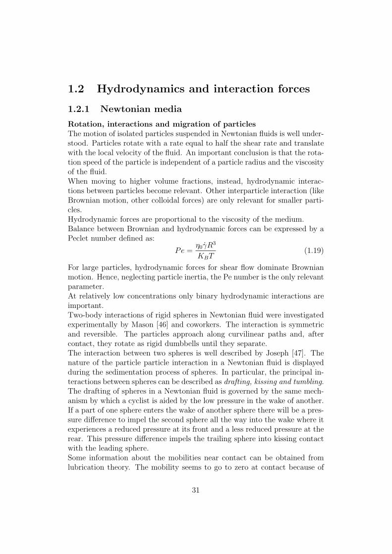
In the work of Michele et al [59], the ratio of the first normal stress differenceover the shear stress which is the Weissenberg number (eq. 1.15), seems tobe the determining factor for the alignment process. In particular, string for-mation seems to occur only if the Weissenberg number exceeds the value of10. Some aspects of the article are however not clear; e.g. the choice of a 100micron gap with particles of 60-70 micron and the subsequent assumptionthat ”the spheres don’t touch the glass plates”.Giesekus [60, 61] showed that in a bidisperse suspension, the particles segre-gate and form separate strings according to the size (see Fig. 1.8).

Figure 1.8: Alignment of a bidisperse suspension in a non-Newtonian liquids[61].

Giesekus also linked the physical origin of string formation to normal forces,thus rationalizing the existence of a critical value for the Weissenberg num-ber.Petit and Noetinger [62] observed particle clusters whose major axis wasaligned in the direction of the applied strain for oscillatory flow.Lyon et al [63] reported experimental results on the evolution of the parti-cle microstructure for non colloidal particles suspended in viscoelastic fluids.In particular they performed monolayer experiments on concentrated suspen-sions (up to 40%) with monodisperse and bidisperse particle size distributionsfor both steady and oscillatory flows.More recently, Scirocco et al [64] investigated the effect of the suspendingfluid on flow-induced alignment by means of microscopy and light scatteringon non colloidal suspensions. They found that the alignment was not gov-erned only by the Weissenberg number. For example, no alignment couldbe observed in constant viscosity, highly elastic Boger fluids, and in slightlyshear thinning Boger fluids the critical Weissenberg number was one orderof magnitude larger than in polymer solutions. Moreover, Scirocco et al [64]studied the kinetics of string formation and the role of the presence of thewalls. They found that the walls seem to hinder rather than promote thealignment and that the alignment can be considered as a bulk phenomenon.

34

Still recently, Kim et al [65] performed monolayer experiments on alignmentand chaining of non-colloidal spherical particles (300 µm) in viscoelastic flu-ids (concentration 10%). As for Scirocco et al [64], particles form string-likestructures even when the normal stress difference is less than the shear stress,proving the hypothesis of the existence of a critical value for the Weissenbergnumber for alignment wrong [59].The mechanism for alignment and chaining is not clearly understood. Themechanism proposed by Jung et al [66] is the most convincing and can beexplained as follows. Before the particles chain, they need to be aligned alongthe flow direction in a flowing suspension. First, alignment was explainedfor the case of two cylinders in a viscoelastic fluid. When the distance be-tween two cylinders is large enough there is no hydrodynamic interactionsand nothing happens. If the two cylinders are placed obliquely and are nearto each other, there is an imbalance due to the fact that the fluid betweenthe cylinders is hindered. In particular, as shown in Fig. (1.9), for the leftcylinder the imbalance will push the left cylinder to the right. For the rightcylinder the reverse is true.

Figure 1.9: Imbalance of shear rate for two cylinders.

This lateral movement will result in the alignment of the two cylinders alongthe flow direction. In the case of a shear thinning fluid the flow between thetwo cylinders will become even weaker due to an increased viscosity causedby the reduced shear rate. This will result in an even smaller shear rates andin a very small value of the normal stress difference. Therefore, in a shearthinning fluid, particles will align more strongly. This mechanism agrees withthe results of Joseph and Feng [56]. They showed that, in case of flow pasttwo spherical particles of the same size along the line connecting their cen-ters, the pressure pushes the particle along the line of centers towards eachother. The alignment of two spheres seems to be very similar to that for two

35

cylinders.

Migration of particles

In addition to alignment and segregation, particle migration occurs in non-dilute systems. While the reason for migration in Newtonian fluids is inertia,there are several reasons for migration in viscoelastic suspensions and thesituation becomes more complex. The term migration refers to lateral mi-gration to the wall, promoted by normal stress differences and shear thinning.The role of normal stress differences on particle migration was elucidated in atheoretical calculation by Brunn [67] and Ho and Leal [68] and in simulationsby Morris and Brady [69]. Migration of particles in non homogeneous shearflow occurs because of a spatially varying shear rate, entailing variations inthe first normal stress difference. The variations in N1 result in a force inthe direction of decreasing shear rate.

Numerous papers concern the cases of Poiseuille and of Couette flows. Es-pecially in the 60’s Mason and coworkers worked on the microrheology ofdispersions both in Newtonian and in non Newtonian media [52, 53]. Variousparticle shapes were considered. These papers provided a precise analysis,both theoretical and experimental, of the trajectories of two or several par-ticles and their hydrodynamic interactions in shear flows.Mason and Karnis [70] found that rigid particles (also not spherical) migratein the direction of decreasing shear rate in Couette and Poiseuille flows forfully viscoelastic fluids. They suggested that this behavior was due to thenormal stress effects of the medium, since migration didn’t occur in Newto-nian fluids.During the same period, Highgate [71] did experiments in a cone plate ge-ometry.Circular rings of high particle concentration that moved outward were ob-served.A series of experiments on particle migration in a plate-plate geometry wereperformed at the Carnegie-Mellon University [72, 73, 74] in Pennsylvania.The migration was observed to be in the direction of decreasing shear rate(inward). Later [72, 74, 75], lateral migration in a Boger fluid was alsostudied. In these fluids the existence of a critical radius in the plate-plategeometry was found; if the distance between the particle and the midpointof the geometry was smaller than this critical radius, migration was directedtoward the axis while there was outward migration when the particle wasinitially located at a distance further from the axis than the critical radius.Along with lateral migration observations were also done for vertical migra-

36

tion: the particles seemed to migrate towards a plane midway between theplates, regardless of the radial migration.Jefri and Zahed [76] observed a chain structure in planar Poiseuille flow ofviscoelastic suspensions of 10%. Experiments were done on three differentmedia, a Newtonian fluid, a Boger fluid and a shear thinning elastic medium.They found that:

• In Newtonian suspensions the particles were uniformly distributed inboth the transverse and axial directions.

• In the shear thinning fluid an immediate migration of particles towardthe upper and lower walls took place. Alignment on the walls was alsoobserved. The minimum concentration of particles was at the centre-line.

• In the constant viscosity elastic fluid (Boger fluid) the particles mostlystationed along the tube axis with very few particles near the upperand lower walls.

The results obtained in this study indicate two important points; first theyconfirm that migration is a consequence of normal stresses and second thatmigration is connected with alignment.Tehrani [77] studied the migration of near spherical particles in pipe flow. Inthe case of a shear thinning fluid with measurable elasticity rapid migrationto regions of lower shear was observed. The highly elastic fluids showedsevere wall slip with no appreciable migration.Feng and Joseph [78] studied the migration of spheres for torsional plate plateflows in viscoelastic fluids. They found that particles migrated outward andtowards the midplane in the vertical direction.

37

Chapter 2

Suspension Rheology

2.1 Materials and Methods

2.1.1 Materials

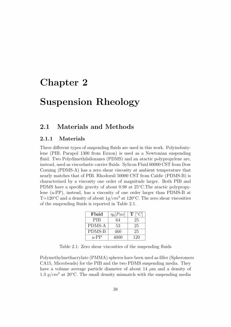
Three different types of suspending fluids are used in this work. Polyisobuty-lene (PIB, Parapol 1300 from Exxon) is used as a Newtonian suspendingfluid. Two Polydimethilsiloxanes (PDMS) and an atactic polypropylene are,instead, used as viscoelastic carrier fluids. Sylicon Fluid 60000 CST from DowCorning (PDMS-A) has a zero shear viscosity at ambient temperature thatnearly matches that of PIB. Rhodorsil 50000 CST from Caldic (PDMS-B) ischaracterized by a viscosity one order of magnitude larger. Both PIB andPDMS have a specific gravity of about 0.98 at 25C.The atactic polypropy-lene (a-PP), instead, has a viscosity of one order larger than PDMS-B atT=120C and a density of about 1g/cm3 at 120C. The zero shear viscositiesof the suspending fluids is reported in Table 2.1.

Fluid η0[Pas] T [C]PIB 64 25

PDMS-A 53 25PDMS-B 460 25

a-PP 4000 120

Table 2.1: Zero shear viscosities of the suspending fluids

Polymethylmethacrylate (PMMA) spheres have been used as filler (SpheromersCA15, Microbeads) for the PIB and the two PDMS suspending media. Theyhave a volume average particle diameter of about 14 µm and a density of1.3 g/cm3 at 20C. The small density mismatch with the suspending media

38

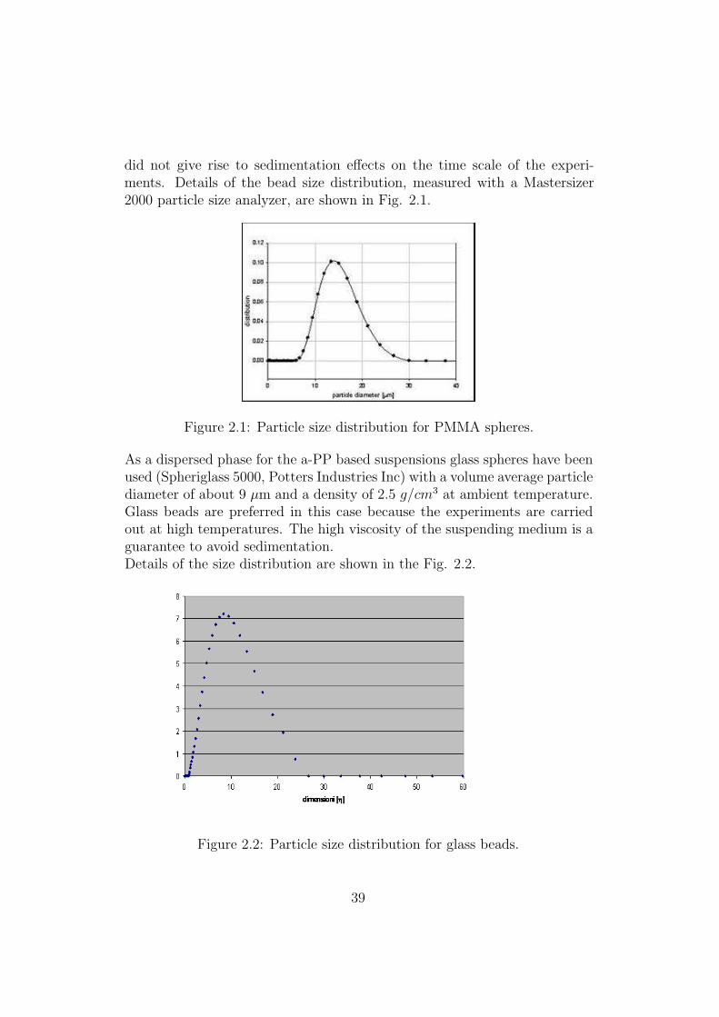
did not give rise to sedimentation effects on the time scale of the experi-ments. Details of the bead size distribution, measured with a Mastersizer2000 particle size analyzer, are shown in Fig. 2.1.

Figure 2.1: Particle size distribution for PMMA spheres.

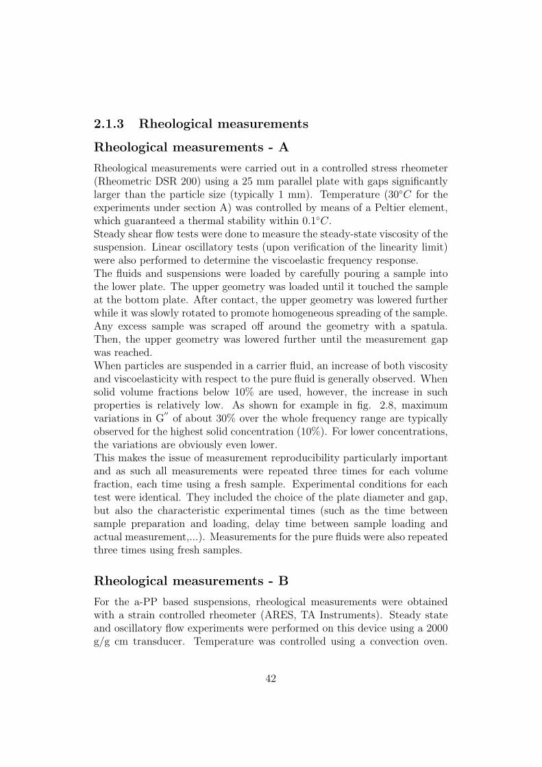
As a dispersed phase for the a-PP based suspensions glass spheres have beenused (Spheriglass 5000, Potters Industries Inc) with a volume average particlediameter of about 9 µm and a density of 2.5 g/cm3 at ambient temperature.Glass beads are preferred in this case because the experiments are carriedout at high temperatures. The high viscosity of the suspending medium is aguarantee to avoid sedimentation.Details of the size distribution are shown in the Fig. 2.2.

Figure 2.2: Particle size distribution for glass beads.

39

2.1.2 Preparation of the suspensions

Preparation of the suspensions was done with care as homogeneous disper-sions of non agglomerated particles are difficult to obtain especially for lowsolid concentrations.To avoid confusion, in this chapter each part contains two sections: in thefirst one, PIB and PDMS based suspensions will be discussed. For thesefluids it is easier to control the volume fraction accurately and the dispersionhas been hand made; in the second section B the a-PP based suspensions thatrequires the use of an extruder to mix particles with fluid will be discussed.

Preparation of suspensions - A

First, the PMMA beads were placed in a vacuum oven pump to remove mois-ture. The polymer and the beads were then weighted and hand mixed in abeaker for 10 minutes in the desired proportion. The air incorporated duringmixing was removed by letting the sample rest for 12 hours. Homogeneous,and at least kinetically stable suspensions, could be obtained using this pro-cedure. Optical microscopy confirmed that the particles were well dispersedand did not form aggregates over long times.In addition, it was checked that in all cases the time scale associated withsedimentation was much larger than the time scale of both sample prepa-ration and experiment. Indeed, Stokes’ law indicates a maximum settlingvelocity (for the least viscous fluid) of about 2µm/hr. The time for PMMAparticles to sediment in the gap of h tickness h= 10−3m of the measurementdevice can be estimated by [18]:

t =0.45η0h

(ρp − ρ0)R2g(2.1)

in which η0 is the viscosity of the pure matrix, R the particle radius and g thegravity constant. ρp and ρ0 are respectively the densities of the suspendedparticles and the suspending medium. In all cases, the time scale associatedwith sedimentation (about 12 h for the lowest viscosity suspending mediumand about 5 days for the more viscous of viscoelastic fluids) was much largerthan the time scale of the experiments. In laminar shear flow the particleReynolds number is defined as follows:

Rep =ρ0R

2γ

η0

(2.2)

As Rep ¿ 1, in all cases particle inertia can be neglected. The particle sizewas sufficiently large to be able to ignore Brownian forces (Pe > 105).

40

Preparation of suspensions - B

The high viscosity requires that the suspensions are prepared by mixing thepolymer with the beads in an extruder (Haake) at 100C for about half anhour. Mixing glass particles with the polymer matrix is not trivial and thereis a significative error on the volume fraction.In order to check the volume fraction of these suspensions, TGA (thermo-gravimetric-analysis) was used.

Figure 2.3: TGA for aPP suspensions.

In Fig. 2.3, the normalized weight is shown as function of temperature. Usingthese data, one can easily calculate the relative volume fraction and make acomparison with the expected volume fraction, as shown in Table 2.2.

Table 2.2: Comparison between required and effective volume fractionsfrom TGA required

2.9 34.5 57.1 711.5 10

41

2.1.3 Rheological measurements

Rheological measurements - A

Rheological measurements were carried out in a controlled stress rheometer(Rheometric DSR 200) using a 25 mm parallel plate with gaps significantlylarger than the particle size (typically 1 mm). Temperature (30C for theexperiments under section A) was controlled by means of a Peltier element,which guaranteed a thermal stability within 0.1C.Steady shear flow tests were done to measure the steady-state viscosity of thesuspension. Linear oscillatory tests (upon verification of the linearity limit)were also performed to determine the viscoelastic frequency response.The fluids and suspensions were loaded by carefully pouring a sample intothe lower plate. The upper geometry was loaded until it touched the sampleat the bottom plate. After contact, the upper geometry was lowered furtherwhile it was slowly rotated to promote homogeneous spreading of the sample.Any excess sample was scraped off around the geometry with a spatula.Then, the upper geometry was lowered further until the measurement gapwas reached.When particles are suspended in a carrier fluid, an increase of both viscosityand viscoelasticity with respect to the pure fluid is generally observed. Whensolid volume fractions below 10% are used, however, the increase in suchproperties is relatively low. As shown for example in fig. 2.8, maximumvariations in G

′′of about 30% over the whole frequency range are typically

observed for the highest solid concentration (10%). For lower concentrations,the variations are obviously even lower.This makes the issue of measurement reproducibility particularly importantand as such all measurements were repeated three times for each volumefraction, each time using a fresh sample. Experimental conditions for eachtest were identical. They included the choice of the plate diameter and gap,but also the characteristic experimental times (such as the time betweensample preparation and loading, delay time between sample loading andactual measurement,...). Measurements for the pure fluids were also repeatedthree times using fresh samples.

Rheological measurements - B

For the a-PP based suspensions, rheological measurements were obtainedwith a strain controlled rheometer (ARES, TA Instruments). Steady stateand oscillatory flow experiments were performed on this device using a 2000g/g cm transducer. Temperature was controlled using a convection oven.

42

Parallel plate geometries have been used (r=12.5 mm, gap∼1 mm). Tem-perature was set at 120C. A waiting time of about 20 minutes after loadingwas used to eliminate the effects of loading history. This waiting time wasa compromise between the time of the sample to ”anneal”, the effects ofloading and the limitations set by the thermal stability of the material.

43

2.2 Experimental results-A

2.2.1 Rheology of suspending fluids

The shear viscosity of suspending fluids is measured using stress sweeps inthe low stress range. All fluids have a constant viscosity in this region. Thevalues are reported in Table 2.1.The linear viscoelastic response of the pure fluids is reported in Figs 2.42.5 and 2.6. For the Newtonian PIB the loss modulus, G

′′, shows a linear

dependence upon frequency for the whole frequency range investigated (0.1-100 rad/s).The elastic modulus, G

′, of the PIB shows an erratic behavior. In particular,

the values for G′

were negative at the lowest frequencies, indicating thatthe elastic modulus was non measurable, within the sensitivity limits of therheometer. Moreover, the Newtonian plateau behavior is observed at allfrequencies. Therefore, we consider PIB as a Newtonian fluid.Both PDMS, on the contrary, show viscoelastic behavior. For them theNewtonian plateau extends up to a frequency of about 1 rad/s.Below these frequencies the typical behavior of the terminal region is observedfor the viscoelastic fluids, with G

′and G

′′characterized by the +2 and +1

slopes, respectively.

Figure 2.4: DFST for Newtonian Polyisobutylene, at 30C.

44

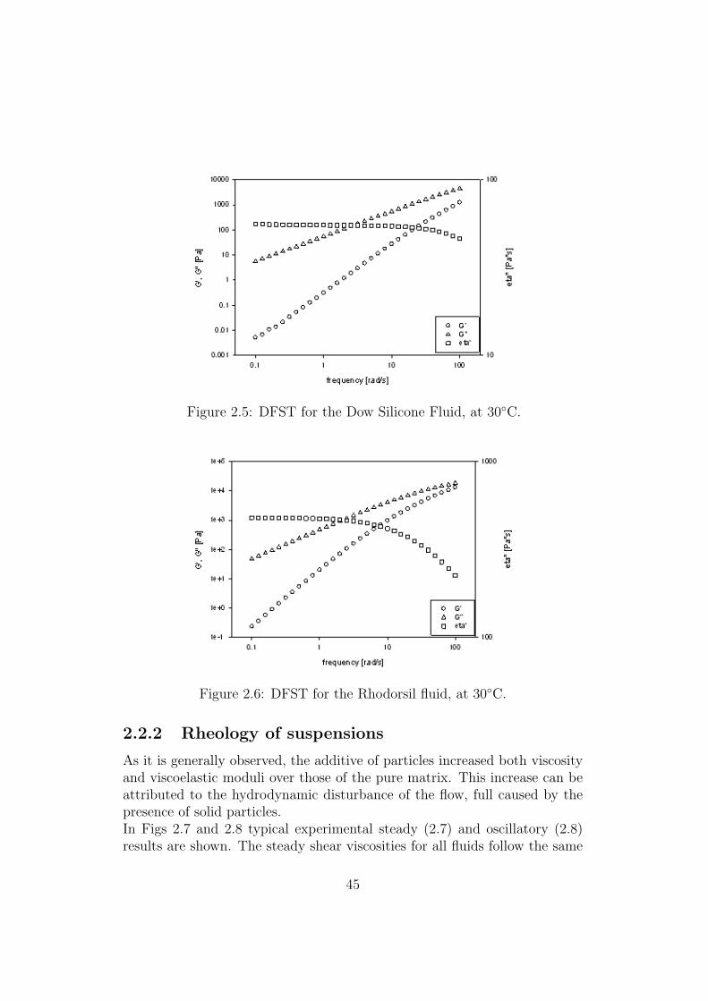
Figure 2.5: DFST for the Dow Silicone Fluid, at 30C.

Figure 2.6: DFST for the Rhodorsil fluid, at 30C.

2.2.2 Rheology of suspensions

As it is generally observed, the additive of particles increased both viscosityand viscoelastic moduli over those of the pure matrix. This increase can beattributed to the hydrodynamic disturbance of the flow, full caused by thepresence of solid particles.In Figs 2.7 and 2.8 typical experimental steady (2.7) and oscillatory (2.8)results are shown. The steady shear viscosities for all fluids follow the same

45

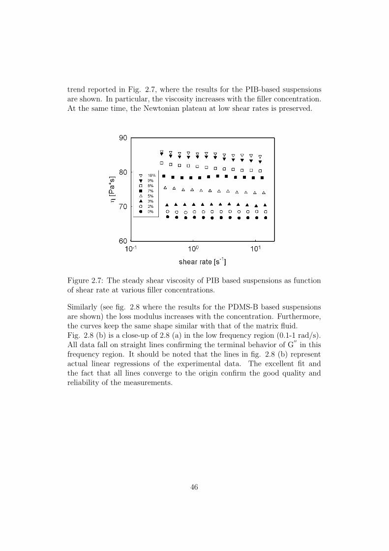
trend reported in Fig. 2.7, where the results for the PIB-based suspensionsare shown. In particular, the viscosity increases with the filler concentration.At the same time, the Newtonian plateau at low shear rates is preserved.

Figure 2.7: The steady shear viscosity of PIB based suspensions as functionof shear rate at various filler concentrations.

Similarly (see fig. 2.8 where the results for the PDMS-B based suspensionsare shown) the loss modulus increases with the concentration. Furthermore,the curves keep the same shape similar with that of the matrix fluid.Fig. 2.8 (b) is a close-up of 2.8 (a) in the low frequency region (0.1-1 rad/s).All data fall on straight lines confirming the terminal behavior of G

′′in this

frequency region. It should be noted that the lines in fig. 2.8 (b) representactual linear regressions of the experimental data. The excellent fit andthe fact that all lines converge to the origin confirm the good quality andreliability of the measurements.

46

Figure 2.8: Loss modulus for PDMS-B based suspensions as function offrequency at various filler concentrations; (a) for all measured frequencies(lines are guides to the eye); (b) in the low frequency range: lines are linearregressions of the data). Symbols as in the Fig. 2.7.

The trends in Fig. 2.8 are similar in all fluids and indicate that in the lowfrequency range (0.1÷1rad/s) the relative increment in rheological propertiesonly depends on the filler concentration. This implies that, in this range, theconcentration dependence of the viscous properties can be robustly checkedin terms of the normalized quantities:

ηn =η

η0

(2.3)

47

G′′n =

G′′

G′′0

(2.4)

in which η is the suspension’s viscosity in the zero-shear plateau at a givenstress and η0 the viscosity of the pure suspending fluid at the same stress;conversely, in equation 2.4, G

′′is the suspension’s loss modulus at a given

frequency and G′′0 the value of the pure matrix at the same frequency.

Dissipative response of suspensions

Figs 2.9-2.11 show the normalized viscosity and loss modulus of the suspen-sions as function of the volume fraction. The error bars in the figure summa-rize the statistical information related to the experimental data. Each pointin the figure represents a large number of measurements. All measurementsfor all concentrations have been repeated on three fresh samples. Further-more, all measurements taken in the above mentioned ranges of shear rateand frequency have been considered. As a consequence, about 45 (for viscos-ity) and 30 (for loss modulus) independent measurements are lumped intoeach data point and its corresponding error bar. In Figs. 2.9 the results forthe PIB Newtonian suspensions are reported. Both the viscosity and the lossmodulus increase non linearly with concentration. It is also confirmed thatfor relatively low concentrations (in this case, for φ<5%), the limiting vis-cosity law of Einstein is well obeyed. Furthermore, the loss modulus followsquantitatively the same behavior as the steady shear viscosity.

Figs 2.10 and 2.11 show the results for the two viscoelastic samples. Thequalitative behavior does not differ from that already observed in Figs. 2.9for the Newtonian suspensions. Quantitatively, however, the deviation fromEinstein’s viscosity law can be seen at lower concentrations with respect tothe Newtonian case. The difference is further enhanced when the solid con-centration increases. On the contrary, when comparing, ηn and G

′′n to each

other, they show a similar behavior.

48

Figure 2.9: Normalized steady shear viscosity (top) and viscous modulus(bottom) for the PIB suspensions as function of volume fraction. Dashedline: Einstein’s viscosity law; solid line: quadratic fit.

49

Figure 2.10: Normalized steady shear viscosity (top) and viscous modu-lus (bottom) for the PDMS-A suspensions as function of volume fraction.Dashed line: Einstein’s prediction; solid line: quadratic fit.

50

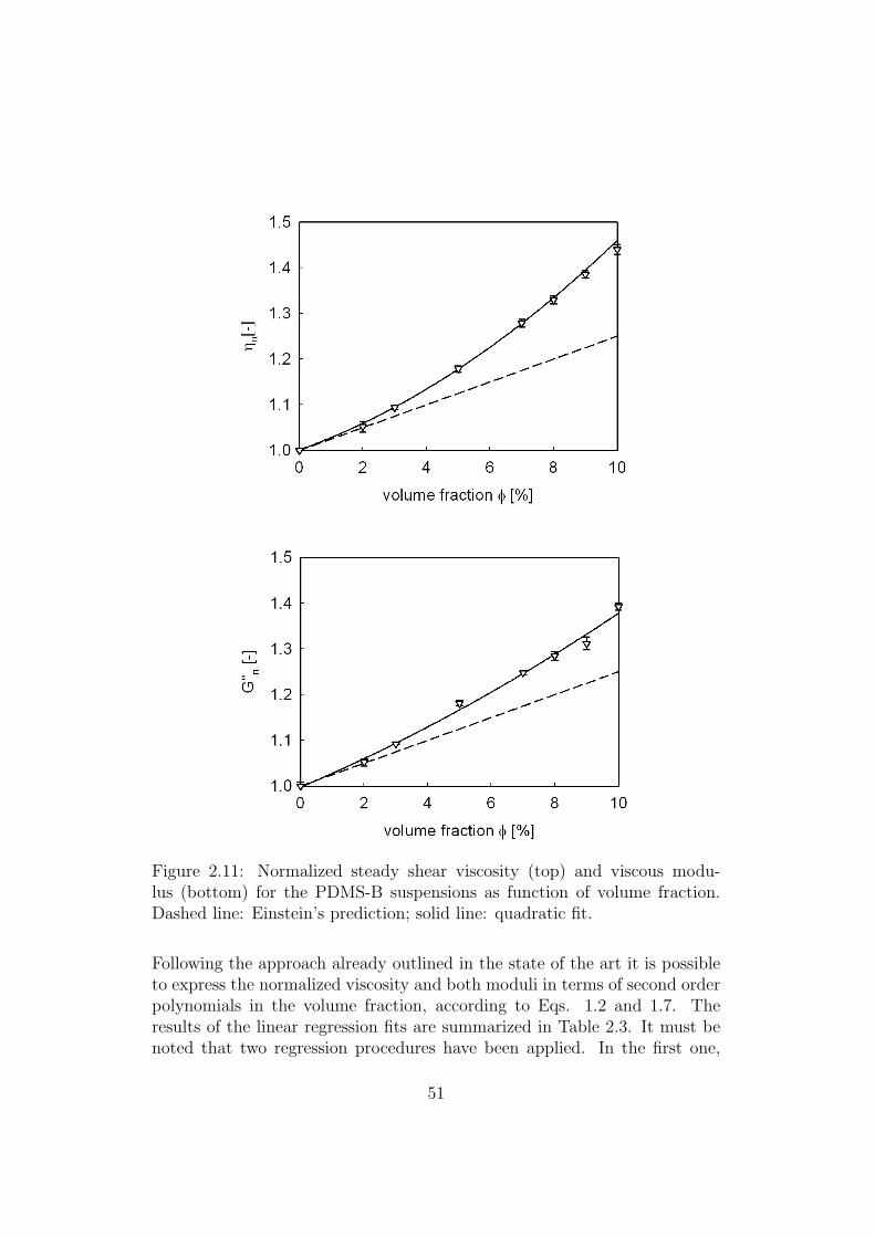
Figure 2.11: Normalized steady shear viscosity (top) and viscous modu-lus (bottom) for the PDMS-B suspensions as function of volume fraction.Dashed line: Einstein’s prediction; solid line: quadratic fit.

Following the approach already outlined in the state of the art it is possibleto express the normalized viscosity and both moduli in terms of second orderpolynomials in the volume fraction, according to Eqs. 1.2 and 1.7. Theresults of the linear regression fits are summarized in Table 2.3. It must benoted that two regression procedures have been applied. In the first one,

51

both first and second order coefficients are free parameters and calculated bythe regression. In the second one, only the second order coefficients (b forthe viscosity and b

′′for the loss modulus) are calculated using the best fit

procedure, the first order coefficients (a and a′′) are kept fixed and equal to

2.5 as predicted by Einstein.

Table 2.3: Fit values of the polynomial coefficients of Eqs. 1.2 and 1.7.Standard deviations are also shown.

Fluid Fit a b a′′

b′′

PIB a and b 2.34±0.07 8.82±0.82 2.47±0.17 7.39±0.85b only 2.5 7.00±0.18 2.5 6.99±0.18

PDMS-A a and b 2.63±0.09 19.5±1.11 2.63±0.07 12.8±0.77b only 2.5 20.9±0.24 2.5 14.5±0.13

PDMS-B a and b 2.67±0.04 17.9±0.51 2.80±0.05 11.1±0.58b only 2.5 19.7±0.15 2.5 14.3±0.13

The polynomial quadratic fits of the experimental data are shown as solidlines in the figures 2.9-2.11. The curves corresponding to the two fit pro-cedures are virtually indistinguishable and in excellent agreement with theexperimental data.It can be noticed that the fit on the first order coefficient is quite robust andalways in good agreement with Einstein’s prediction for dilute suspensions.In fact, even when a and a

′′are calculated through regression, the maximum

deviation from the theoretical value of 2.5 is 11%. The 2.5 value is confirmedfor both the Newtonian and viscoelastic suspensions, as theoretical demon-strated [29].As far as the second order coefficients are concerned, Table 2.3 shows thesubstantial difference in behavior between the Newtonian and viscoelasticsuspensions.

The b and b′′

values for the Newtonian PIB fluid are in excellent quanti-tative agreement with Batchelor’s exact calculations (which is valid for elon-gational viscosity). The results for the Newtonian PIB matrix are also ingood quantitative agreement with the experimental results of Saunders [15],who measured the shear viscosity of sub-micron size polystyrene latex sus-pensions. The results are also consistent with those of Highgate and Whorlow[39] for PMMA beads (average diameter of 100 µm) suspended in a Newto-nian synthetic oil. The results also agree with the simulations of particles inboth Newtonian and non-Newtonian fluids by Hwang et al [23] and Hwangand Hulsen [24]. In these simulations of circular inertialess disks in New-

52

tonian fluids a deviation from the limiting linear behavior appear when thearea fraction exceeds about 5%; moreover a deviation of about 4% is shownfor an area fraction of about 10%, that is our highest solid concentration.This implies a second order factor equal to about 4 (not far from Bacth-elor’s result even if the simulation is 2D). Moreover, our results confirm thatthe bulk shear viscosity increases with elasticity [23] [24]. The second orderpolynomial coefficients of the two viscoelastic suspensions are, indeed, signif-icantly larger.Significantly larger values of the second order coefficient of the viscoelasticsuspensions are obtained either leaving the first order coefficient as a freeregression parameter or keeping it fixed to 2.5. The effect seems somewhatless pronounced for the loss modulus than for the viscosity. It can be con-cluded that, out of possible experimental error, the viscoelastic suspensionsshow larger deviations from linearity in the semidilute regime than those ofthe Newtonian suspensions. An overall comparison between the polynomialpredictions and the experimental data is presented in Fig. 2.12. Here, datahave been replotted in terms of (η−η0)/(η0φ) and (G

′′−G′′0)/(G

′′0φ) , as done

for example by Saunders [15], in order to single out the deviations from lin-earity due to the quadratic term. The different behavior between Newtonianand viscoelastic suspensions can be again clearly appreciated, as well as thegood quantitative agreement between the experimental data and the secondorder polynomial fit.

53

Figure 2.12: Intrinsic steady shear viscosity (top) and intrinsic loss modulus(bottom) for the three suspensions as function of volume fraction

54

Elastic behavior of suspensions

The elastic moduli for the two PDMS viscoelastic fluids are much smallerthan the corresponding loss moduli, as can be seen in Figs 2.5 and 2.6. As aconsequence, the experimental data for G

′and their dependence upon solid

concentration are much less reliable and reproducible than the correspondingresults for G

′′. Hence, the dependence of the storage modulus on volume

fraction is not so easy to determine with the same accuracy in particularin the low frequency range. At low frequencies, indeed, the stress signalleads phase angle shift by π/2; the ratio of the viscous modulus to the elasticmodulus (the tangent of the phase angle shift between stress and strain) turnsinto ∞ and the determination of storage modulus is more affected by errors.This is shown in Fig. 2.13. With a Dynamic Point Test, ten points are takensequentially at a certain frequency, and this for different frequencies. TheFig. 2.13 shows that the experimental error which is the standard deviationon the mean value increases with decreasing frequency. Whereas the erroron the loss modulus is quite the same in the whole frequency range, the erroron the storage modulus increases with decreasing frequency with more thanone order of magnitude.

Figure 2.13: The percent error for three different frequencies (0.1, 1 and 10rad/s), for both the calculation of G

′() and G

′′(5)

To examine the influence of frequency and polymer molecular weight on therelative behavior of G

′and G

′′as filler volume fraction is increased, we plot

the ratio of G′′

G′ , versus frequency.

55

In fig. 2.14, trends of tanδ=G′′/G

′is shown as function of frequency for our

viscoelastic suspensions.

Figure 2.14: The ratio of the loss over the storage modulus versus frequencyfor filled and unfilled PDMS fluids.

56

As the molecular weight of the polymer increases, the magnitude of G′′/G

′

decreases at all frequencies and shows a monotonic decrease with increasingfrequency at all volume fractions.As shown by Walberer and McHugh [44], the decrease in G

′′/G

′at a given

frequency indicates that material elasticity (as quantified by G′) grows more

rapidly with molecular weight than the material dissipative behavior (asquantified by G

′′). Furthermore, as frequency increases, the materials be-

come more elastic and tan(δ) decreases. Fig. 2.14 demonstrates that G′′/G

′

for different molecular weight PDMS is identical for all filler amounts in thefrequency range 1-100 rad/s. Moreover, with increasing the molecular weightPDMS systems, the presence of the filler seems to have no influence on theG′′/G

′ratio both in the high and low frequency range.

This behavior was explained by Walberer and McHugh [44] in terms of therelative effect of the filler on the Deborah number of the system: ”The effectof an increase in filler amount is to increase the elasticity of the materialand therefore increase the average relaxation time of the material. At highfrequencies, the Deborah number is quite large and the unfilled material ex-hibits elastic dominated behavior. Therefore the addition of more elasticityto the material with the addition of filler has relatively little effect on theDeborah number. The behavior is quite different at low frequencies how-ever.”Our results agree with those of Walberer and McHugh [44] with regards tothe dependence on molecular weight. Our findings are however different fromtheir generic trend in which the value of G

′′/G

′is shown to decrease as filler

amount is increased.This is ensured by a random sequence of data of tan(δ) in the low frequencyrange, with no obeying to a specific law in the volume fraction.Moreover, if viscoelastic moduli are an increasing function of volume fraction,the constant value of tan(δ) at each frequency suggests the possibility of anoverlap of G

′′(φ) and G

′(φ), in contrast with at least two works in literature

[40, 42].The possibility to use the same functions for the viscoelastic moduli suggeststhat:

• by adding particles G′′

and G′shift only vertically.

• One can calculate a polynomial function of normalized values, useful forboth G

′′and G

′, that represents the dependence of viscoelastic moduli

on frequency at least in the high frequency range.

In fig. 2.15, comparison between data in the low frequency range and datain the whole frequency range is shown. Fits in both cases have been made.

57

In the low frequency range, the result are those reported in tab 2.3; for thewhole frequency range (100-0.1 rad/s), the regression line for the PDMS-Bbased suspensions is plotted in fig. 2.15. The difference between the fit inthe low frequency range and in the whole frequency range is neglectable. Theerror bars are calculated as explained before.

Figure 2.15: Comparison between normalized viscous modulus for PDMSbased suspensions in the low frequency range and in the whole frequencyrange. Line is the best fit to data.

By quantitatively calculating both fits, one can conclude the following:

• The fit on the first order coefficient is quite robust and always in goodagreement with Einstein’s prediction for dilute suspensions.

• The curves corresponding to the two fit procedures are virtually indis-tinguishable and in excellent agreement with the experimental data,meaning that the curve of G

′′shifts only vertically when particles are

added to the pure suspending fluids.

• The possibility to use also the high frequency range suggests to fit dataof storage modulus in the range [1-100] rad/s. In this way, it is possibleto avoid the problem of sensitivity of the instrument and confirm thesame scaling with volume fraction for storage and loss moduli.

58

Following the lines of the previous discussion, the normalized storage in thefrequency range [1-100] rad/s is shown in Fig. 2.16. When going fromthe PDMS-A (top) to PDMS-B (bottom) based suspensions, the molecularweight of the suspending medium increases.

Figure 2.16: Relative storage modulus as function of volume fraction for thesuspending media. The lines are best fits to the data.

59

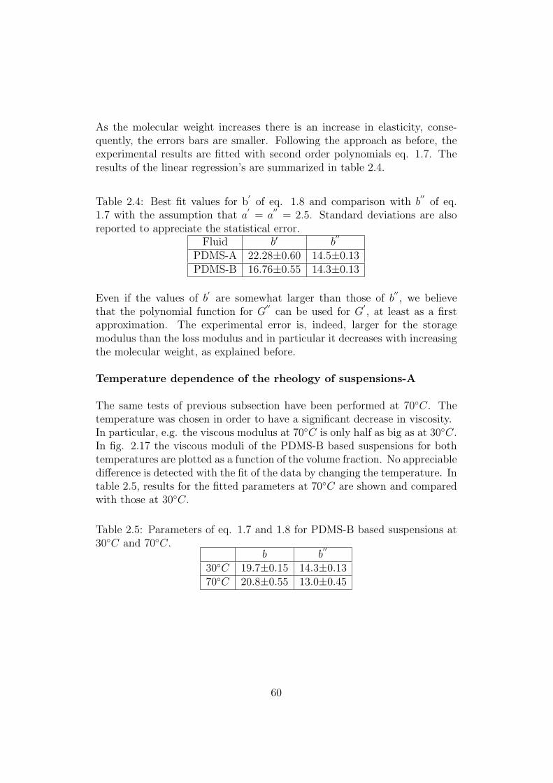
As the molecular weight increases there is an increase in elasticity, conse-quently, the errors bars are smaller. Following the approach as before, theexperimental results are fitted with second order polynomials eq. 1.7. Theresults of the linear regression’s are summarized in table 2.4.

Table 2.4: Best fit values for b′

of eq. 1.8 and comparison with b′′

of eq.1.7 with the assumption that a

′= a

′′= 2.5. Standard deviations are also

reported to appreciate the statistical error.Fluid b′ b

′′

PDMS-A 22.28±0.60 14.5±0.13PDMS-B 16.76±0.55 14.3±0.13

Even if the values of b′

are somewhat larger than those of b′′, we believe

that the polynomial function for G′′

can be used for G′, at least as a first

approximation. The experimental error is, indeed, larger for the storagemodulus than the loss modulus and in particular it decreases with increasingthe molecular weight, as explained before.

Temperature dependence of the rheology of suspensions-A

The same tests of previous subsection have been performed at 70C. Thetemperature was chosen in order to have a significant decrease in viscosity.In particular, e.g. the viscous modulus at 70C is only half as big as at 30C.In fig. 2.17 the viscous moduli of the PDMS-B based suspensions for bothtemperatures are plotted as a function of the volume fraction. No appreciabledifference is detected with the fit of the data by changing the temperature. Intable 2.5, results for the fitted parameters at 70C are shown and comparedwith those at 30C.

Table 2.5: Parameters of eq. 1.7 and 1.8 for PDMS-B based suspensions at30C and 70C.

b b′′

30C 19.7±0.15 14.3±0.1370C 20.8±0.55 13.0±0.45

60

Figure 2.17: Comparison between data of viscous modulus for PDMS-B basedsuspensions at 70C with those at 30C.

There is a good agreement between the fitting parameters at the two tem-peratures.The temperature affects only the properties of the pure suspending media,meaning that, when considering normalized values, the dependence of therheological properties on temperature is not relevant anymore.Moreover, the data at 70C have larger error bars. This can be explained witha worse sensitivity rheometer, due to the decreasing of measured torques, aswell as to the decreasing of the viscosity, which means faster sedimentationof the particles (eq.4.1) and, as such, less stable suspensions.

61

2.3 Experimental results-B

2.3.1 Rheology of atactic-polypropylene

Fig. 2.18 shows the viscoelastic behavior for the a-PP suspending medium.The Newtonian plateau extends only until 0.1 rad/s. The terminal region isobserved, with G

′and G

′′characterized by the +1 and +2 slopes, respectively.

Figure 2.18: DFST for pure suspending atactic polypropylene

2.3.2 Rheology of the suspensions

As already said, the values of b that we found are different for Newtonianand viscoelastic suspending liquids. We attributed this to the elasticity ofthe suspending media.However, the visco-elastic suspending fluids used before are both PDMS liq-uids and are chemically as well as rheologically not very different. That iswhy the coefficients b

′′(and b) are almost equal for these fluids.

The question is: how does b′′

(and b and b′) depend on the rheological

properties of the suspending matrix? In order to answer this question, thedependence of the viscoelastic moduli on volume fraction was studied foratactic polypropylene based suspensions, as shown in fig. 2.19.

62

Figure 2.19: Loss (a) and storage (b) moduli for a-PP based suspensions asfunction of frequency at various filler concentrations.

As for the previous suspending media, G′′

and G′

increase with increasingvolume fraction. It is impossible to perform experiments with the sameaccuracy as before, because on one hand the accuracy on volume fractionis lower (see section 2.1.2) and, on the other hand, the rheology tests areperformed at high temperature, with more difficulties to check and controlthe test conditions.

63

The normalized viscous and storage moduli are plotted as function of thereal volume fraction in figs. 2.20 and 2.21.

Figure 2.20: Normalized viscous modulus for the a-PP suspension as functionof bead volume fraction.

Figure 2.21: Normalized storage modulus for the a-PP suspension as functionof bead volume fraction.

64

Even without the high accuracy, it can be easily seen that the increase in G′′

and in G′with increasing volume fraction is larger for the atactic polypropy-

lene based suspensions than PDMS based suspensions, and definitely largerthan the Newtonian case.For example, in fig. 2.20, at a frequency of 1 rad/s, the increase in G

′′when

volume fraction changes from 3% to 10% is about 300%, in comparison toabout 30% for the same volume fractions for the PDMS suspensions.The normalized complex viscosity seems to have the same dependence of theviscous modulus.This behavior can be explained again with the higher elasticity of the sus-pending medium and, perhaps, with a different chemical structure of thefluid.The elastic modulus seems to have a stronger dependence on volume frac-tion than the viscous modulus as shown in fig. 2.21 in contrast with resultsobtained for PDMS based suspensions.Some experiments on the first normal stresses difference (N1) have been per-formed on the a-PP based suspensions. Results for N1 as a function of shearrate are shown in fig. 2.22 for different volume fractions.

Figure 2.22: N1 as function of shear rates for different volume fractions.Symbols as in Fig. 2.20.

In agreement with previous literature [34] [79] [80] [36] [28] [23], using vis-coelastic suspending fluids at moderate volume fractions, we find that thefirst normal stress difference increases with increasing solid content, when

65

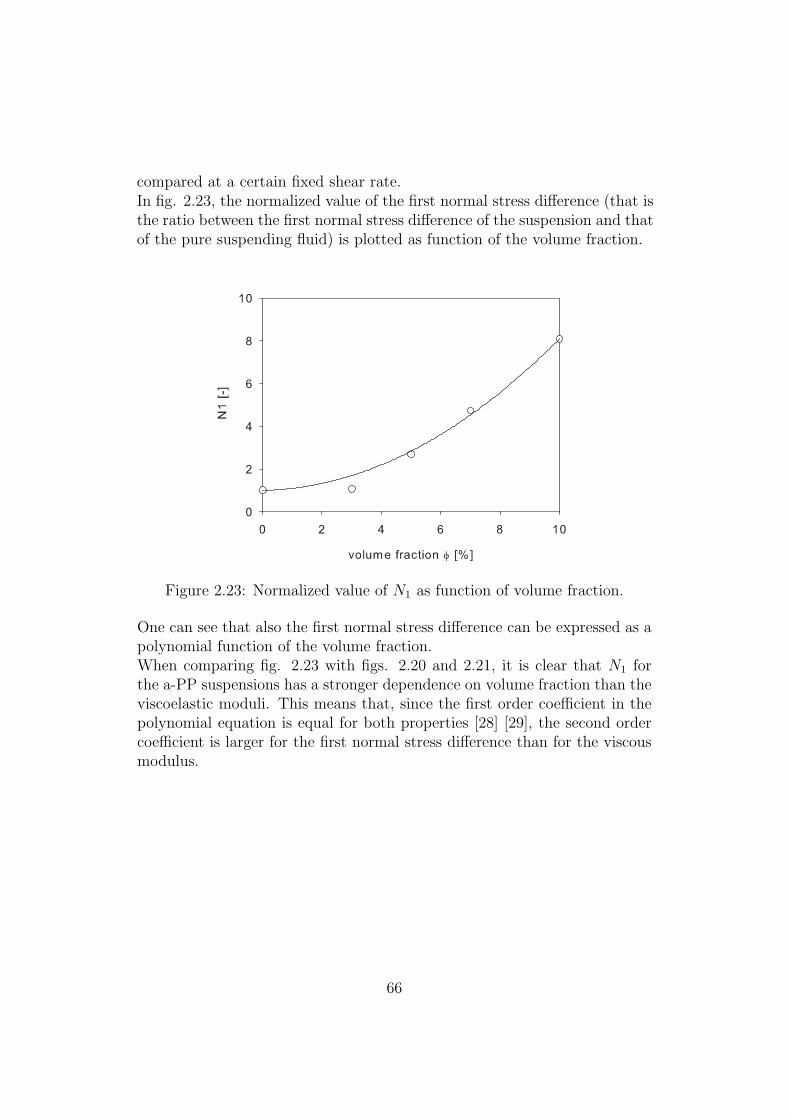
compared at a certain fixed shear rate.In fig. 2.23, the normalized value of the first normal stress difference (that isthe ratio between the first normal stress difference of the suspension and thatof the pure suspending fluid) is plotted as function of the volume fraction.

Figure 2.23: Normalized value of N1 as function of volume fraction.

One can see that also the first normal stress difference can be expressed as apolynomial function of the volume fraction.When comparing fig. 2.23 with figs. 2.20 and 2.21, it is clear that N1 forthe a-PP suspensions has a stronger dependence on volume fraction than theviscoelastic moduli. This means that, since the first order coefficient in thepolynomial equation is equal for both properties [28] [29], the second ordercoefficient is larger for the first normal stress difference than for the viscousmodulus.

66

2.4 Conclusions

In this chapter the rheology of suspensions of particles in different suspendingmedia has been studied. The influence of the medium on the rheological re-sponse of the suspensions has been investigated in the dilute and semi-diluteregions.To our knowledge, this is the first experimental study comparing the rheo-logical behavior of Newtonian and viscoelastic suspensions in the semidiluteconcentration range as function of volume fraction. In this range, parti-cle/particle hydrodynamic interactions are relevant and determine a sub-stantial deviation from the limiting dilute behavior.The experimental measurements show that in the semi-dilute regime the de-pendence of the linear viscoelastic properties of the suspensions can be welldescribed with a quadratic polynomial.For Newtonian suspensions, the experimental data agree quantitatively wellwith the analytical hydrodynamic calculations performed by Batchelor [5].However, Batchelor’s results are for irrotational flows. The limiting behav-ior in the dilute regime predicted by the exact equation of Einstein [2] forNewtonian fluids and Palierne [29] for viscoelastic fluids is well obeyed bythe investigated suspensions.In the semidilute regime, viscoelastic suspensions display substantial devia-tions with respect to the Newtonian case. In particular, the deviation fromlinearity of the dissipative properties in the semi-dilute regime is found tobe larger when compared to that of the Newtonian-based suspensions. Thiswas verified at two different temperatures, 30C and 70C.For the viscoelastic fluids, the dependence on volume fraction seems to bevalid for the whole frequency range: adding particles only shifts the curvesvertically.Furthermore, tan(δ) confirms that the storage and loss moduli have the samedependence on volume fraction.Finally, the study of the first normal stress difference shows that the depen-dence on volume fraction is stronger (a larger deviation from linearity) thanthe dependence of the viscous modulus.The most important result of this chapter is that the nature of the suspend-ing fluid is responsible for changes in the rheological response of suspensions,in shear and oscillatory tests, at second order in φ.Moreover, in order to compare with existing simulations on viscoelastic sus-pensions, we calculated the Weissenberg number as the product of the shearrate and the longest relaxation time [81]. Herein, the longest relaxation timewas considered the inverse of the frequency at which the viscous modulusdeviates from its terminal region behavior (slope 2).

67

The longest relaxation time for the different viscoelastic suspending media,calculated with this method, are shown in tab. 2.6.

Table 2.6: Longest relaxation time λmax for the suspending media.

Fluid λmax

PDMS-A 0.03PDMS-B 0.2

a-PP 3.00

In fig. 2.24 the intrinsic viscous modulus is shown as function of the longestrelaxation time, for different volume fractions.

Figure 2.24: Normalized viscous modulus as function of the longest relaxationtime λmax for the three suspending media, for different volume fractions.

The increase of the viscous modulus at a certain volume fraction is muchhigher for the suspending media with a larger relaxation time (or Weissenbergnumber). This result is in agreement with simulations [23].At this moment, there is no definite explanation for the observed differencebetween Newtonian and viscoelastic suspensions. Certainly, this differenceoriginates from the complex, time dependent flow in the viscoelastic fluidbetween two nearby particles. Efforts are needed to elucidate the hydrody-namic interactions between two particles and their consequent effect on therheological response of viscoelastic suspensions.

68

Chapter 3

Simulation of circular disks in aNewtonian fluid under 2-Doscillatory flow

Computational fluid dynamics is currently very popular because informa-tion implicit in the equations of fluid motion can in principle be extractedwithout approximation using numerical simulations. The potential for solid-liquid flows is very big and has yet to be fully realized.In the last two decades the rheological behavior of suspensions has beenintensively investigated using computer simulations. However, literature fo-cuses mainly on flow simulations of Brownian (colloidal) systems [82], andnot so much on non-Brownian suspensions.For simulations of fluid-solid systems at finite Reynolds number, quite samenumerical methods have been developed in recent years. One of the mostused methods is the ALE (Arbitrary Lagrangian Eulerian) particle mover.The ALE particle mover uses a technique based on a combined formulationof the fluid and particle momentum equations, together with an arbitraryLagrangianEulerian (ALE) moving, unstructured, finite-element mesh tech-nique to deal with the movement of the particles. It was developed by Huand co-workers [83], [84]. The method has been used to solve particle mo-tions under flow in both Newtonian and viscoelastic fluids in two and threedimensions flow geometries. It can describe particles of different size, shape,and material.Recently, Hwang et al [23] [24] simulated the motion of circular inertialessdisks under flow particles in Newtonian and viscoelastic fluid. The bulk shearand elongational viscosity as function of solid area fraction and Weissenbergnumber for a wide range of area fractions were calculated. For small solidarea fractions, the shear viscosity was found to converge to Einstein’s ana-

69

lytical result for a dilute suspension of circular disks [26] [85]. For larger areafractions, both the elongational and shear viscosity show the same quanti-tative deviation from the dilute case. Furthermore, the viscosity was foundto be an increasing function of the Weissenberg number, implying a shearthickening behavior of the suspension.As far as we know, no simulations have been done to investigate the depen-dence of the viscoelastic moduli on volume fraction.In this section, we describe simulation for non Brownian hard particle sus-pensions formulated with a Newtonian fluid under oscillatory shear flow ina well defined domain. Concentrating on circular disks in two-dimensionalflows of a Newtonian fluid, we will demonstrate the feasibility of our schemefor the single sphere as well as the two particle problem.This chapter is organized as follows: first, the governing equations and theboundary conditions are stated. Next, the assumptions are discussed. Fi-nally, the two different example problems will be discussed along with theevaluation of bulk rheological properties.

3.1 Modeling aspects

Consider an incompressible fluid occupying a bounded region Ω with bound-aries Γi, i=1,...4. There are one or two particles freely moving in the fluid.We are interested in the motion of both the fluid and the individual solidparticles and, in particular, the dependence of viscosity on volume fraction.The model consists of a fluid part, solved with the Navier-Stokes equationsin the flow channel, and a structural mechanics part, which it is solved acrossthe particle. Moving Mesh (ALE) application mode makes sure that the flowdomain is deformed along with the particle. Transient effects are taken intoaccount in both fluid and structure.The particles move because of the imposed flow and hydrodynamic interac-tions: their rigid-body motion is completely defined by their translationalvelocity, Ui and their angular velocity, wi = wik, where k is the unit vectorin the normal direction to the xy plane.We restricted the calculations to 2-D systems composed of circular disks in aNewtonian fluid. However, the present scheme can be probably extended toviscoelastic fluids without too much further effort [23]. However, extendingto three-dimensional flow seems more difficult and only limited informationabout this is available.The motion of the fluid satisfies the conservation of mass equation:

∇ · u = 0 (3.1)

70

and the conservation of momentum equation:

ρ∂u

∂t−∇σ + ρ(u · ∇)u = ρf (3.2)

where u is the velocity vector, ρ the density of the fluid, f the body force andσ the stress tensor.For a Newtonian fluid the stress tensor is given by the simple constitutiveequation:

σ = −pI + η0[∇u + (∇u)T ] (3.3)

where I is the unit diagonal matrix, p the pressure and η0 the viscosity ofthe fluid. We assume that gravitation nor other body forces are working onthe fluid, so f = 0.The fluid boundary condition are given by:

u = Ui + wi × (x−Xi) (3.4)

u = γ0ωycos(ωt) v = 0 (3.5)

Eq. 3.4 describes the rigid-body condition, x are the coordinates of the pointson the particle surface, Xi=(Xi, Yi) are the coordinates of the particle centerand Ui = (Ui, Vi) are the components of the translational velocity. Eq. 3.5describes the oscillatory flow boundary condition, with ω the frequency, γ0

the deformation and y the distance from the center of the square. The Carte-sian x and y coordinates are selected such that the origin is at the center ofthe domain, so everything is oscillating.In absence of inertia, no initial conditions are needed for the velocity field ofthe fluid and the motion of particles.Usually the particle is considered as a rigid ring, filled with the same fluid asthe fluid domain so that the rigid-body condition is imposed on the particleboundary only. This rigid-ring description is possible when inertia is negli-gible and is particularly useful because it saves memory.We decided to consider the particle as a structural mechanics part [86], but,as inertia is neglected, the evaluation of the stress can be carried out withthe same procedure as in the rigid-ring description.The motion of solid objects satisfies Newton’s law, in which the force thatmakes the particles move is that imposed by the fluid. The movement ofparticles is given by the following kinematic equations:

dXi

dt= Ui (3.6)

dΘi

dt= wi (3.7)

71

(with the corresponding initial values) where Xi=(Xi, Yi) are the coordinatesof the particle center and Θi is the angular velocity.To determine the unknown rigid motions of the particles, one needs to balancethe drag forces and torques on the particle boundaries. Neglecting inertia andother external forces and torques, the particles are force-free and torque-freeand the balance equations can be written as:

Fi =

∫

Api

σ · nds = 0 (3.8)

Ti =

∫

Api

(x−Xi)× σnds = 0 (3.9)

In these equations, Fi and Ti are the total force and torque on the particleboundaries and n is the outward directed unit normal vector on each part ofthe boundary Api of the particle.

The model geometry consists of a square box in which a Newtonian fluid isforced to move in an oscillatory way and in which one or at maximum twoparticles are dispersed.The non-dimensional parameters governing this flow problem are:

• the relative channel width and length normalized using the particle sizeL/D, which have to be large enough to avoid wall effects (minimum 10for 0.25% calculation error).

• the solid area fraction φa = NπD2

4L2 with N the number of particles presentin the fluid 1 or 2.

In our system the box in which the fluid and particles are forced to moveis square (L in fig. 3.1). The fluid is assumed to be Newtonian, having adensity equal to zero and a viscosity of η0=1 Pa·s.The particles are assumed to be rigid with a density equal to zero. Theparticle size (D in fig. 3.1) is changed in order to have L/D ratios from 10.4to 26.

72

Figure 3.1: The geometry used in the simulation technique.

3.2 Bulk stress

As previously discussed, we are interested in the rheological properties ofdilute and semi-dilute suspensions in oscillatory flow, such as the viscousmodulus.The flow and stress fields obtained from the equations just presented arelocal. Local values of pressure and velocity are directly related to the stressdistribution around the particles and provide information about the hydro-dynamic interaction between the particles.However, it is also important to evaluate global properties (bulk properties)to be able to make predictions for the global behavior of the material.To be able to evaluate global properties, we have to calculate the bulk stressfrom the local quantities. The bulk stress, which is the average stress overthe domain, can be expressed, for a volume V, as the sum of the fluid contri-bution and the particle contribution. We will consider Batchelor’s formula[87]. For 2D, the bulk stress tensor can be calculated as follows:

< σ >=< σ >f + < σ >p=1

A

∫

Af

σdA +1

A

∫

Ap

σdA (3.10)

where the symbol <> means an average over an area A, Af and Ap arerespectively the area occupied by the fluid and the particles.For a Newtonian fluid, the fluid contribution is given by Eq. 3.3 and theshear stress can be easily calculated. Concerning the particle contribution itcan be shown that the integral over the total particle area for the stress canbe written as follows:

< σ >p= (σxxnx + σxyny)nyD

2(3.11)

n being the outward directed unit normal vector on the particle boundary(in the x or in the y direction) and σxx and σxy components of the stress inthe designated directions.

73

3.3 The single particle problem

The first test problem is a single particle of diameter D suspended freelyat the center of the described domain. As mentioned earlier, the referencevelocity is zero at the center of the domain. As such the upper boundarytranslates with a velocity L/2γ and the lower one translates at the velocity−L/2γ, γ being the externally imposed shear rate. As such the particle willnot translate relative to the domain but rotates with an angular velocityw(t).The externally imposed oscillatory deformation is given by:

γ = γ0ωcos(ωt) (3.12)

with γ0 being the amplitude of deformation (set equal to 10%) and ω theoscillation frequency.By changing the L/D ratios from 10.4 to 26, the maximum available volumefraction ranges from 0.1% to 0.8%.The problem of the dynamics of a single sphere immersed in a linear flowfield imposed at infinity, in the absence of both fluid and particle inertia,was first addressed by Einstein [88] for the case of a Newtonian suspendingmedium. Under shear flow, the sphere translates in the flow direction, whilerotating around the vorticity axis. Einstein demonstrated that, with no-slipboundary conditions at the particle surface, the rotation rate of the sphereis w = γ/2. This simple result stems from a torque balance at the spheresurface, whereby the torque on the sphere is only due to the flow field (theso called torque-free condition presented before).To check our model, we measured the rotation rate of one particle in the caseL/D=26 (see fig. 3.1) changing the frequency from 0.1 to 100 rad/s. Becausethe suspending fluid is Newtonian, the rotation rate should not change withfrequency (see fig. 3.2).

74

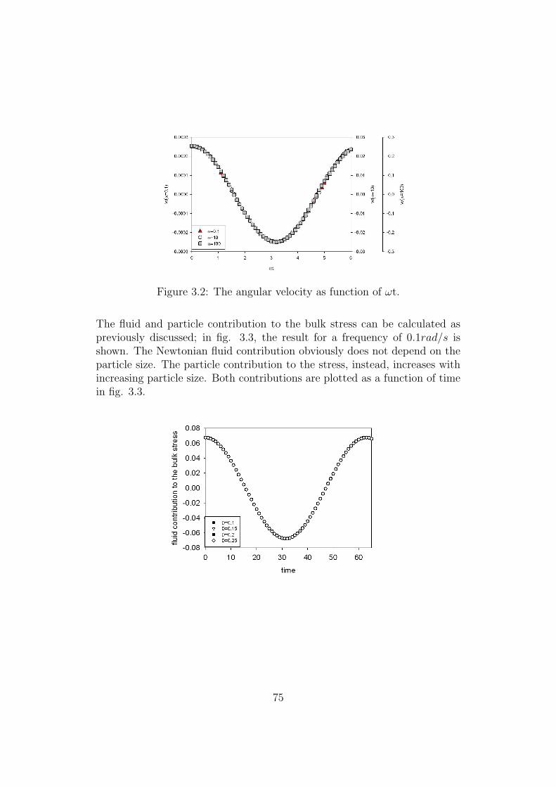
Figure 3.2: The angular velocity as function of ωt.

The fluid and particle contribution to the bulk stress can be calculated aspreviously discussed; in fig. 3.3, the result for a frequency of 0.1rad/s isshown. The Newtonian fluid contribution obviously does not depend on theparticle size. The particle contribution to the stress, instead, increases withincreasing particle size. Both contributions are plotted as a function of timein fig. 3.3.

75

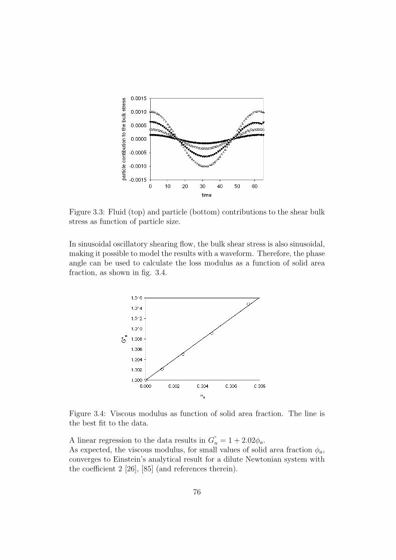
Figure 3.3: Fluid (top) and particle (bottom) contributions to the shear bulkstress as function of particle size.

In sinusoidal oscillatory shearing flow, the bulk shear stress is also sinusoidal,making it possible to model the results with a waveform. Therefore, the phaseangle can be used to calculate the loss modulus as a function of solid areafraction, as shown in fig. 3.4.

Figure 3.4: Viscous modulus as function of solid area fraction. The line isthe best fit to the data.

A linear regression to the data results in G”n = 1 + 2.02φa.

As expected, the viscous modulus, for small values of solid area fraction φa,converges to Einstein’s analytical result for a dilute Newtonian system withthe coefficient 2 [26], [85] (and references therein).

76

3.4 The two particles problem

The two-particle problem is simulated to investigate the effect of the hydro-dynamic interactions between two particles. Two identical particles, withdiameter D, are suspended freely in the domain.Again, the reference velocity is zero at the center of the domain. We dividedthe domain in four sub-domains and investigated the approach between theparticles only in one of them by changing the interparticle distance. One candiscard the other subdomains for symmetry reasons.Hence, the distance between the particles can be seen as the strength of thehydrodynamic interactions between the particles.

One particle is placed in the center of the domain, as before. As such, itcan rotate freely but it will not translate. The other particle is placed inone of the four sub-domains and its initial position is changed randomly. Inparticular, as shown in fig. 3.5, the red particle will start moving to the rightand then moving to the left, following the sinusoidal strain. To increase thevolume fraction while avoiding influences of the walls, one can translate thechosen sub-domain towards the center.For each particle size, about twenty initial configurations are studied, chang-

Figure 3.5: The division of the domain box in four sub-domains; one particleis in the center of the box; the initial position of the other particle is changed.

ing the distance between the two spheres both horizontally and vertically.The bulk stress is always larger than one; it goes through a maximum whenthe particles are very close together and becomes minimum when they arefar apart.The bulk stresses, and consequently the viscous moduli, are calculated forall configurations; the final value for the viscous modulus at a certain solidarea fraction is the mean of all configurations.The result is shown in fig. 3.6.

77

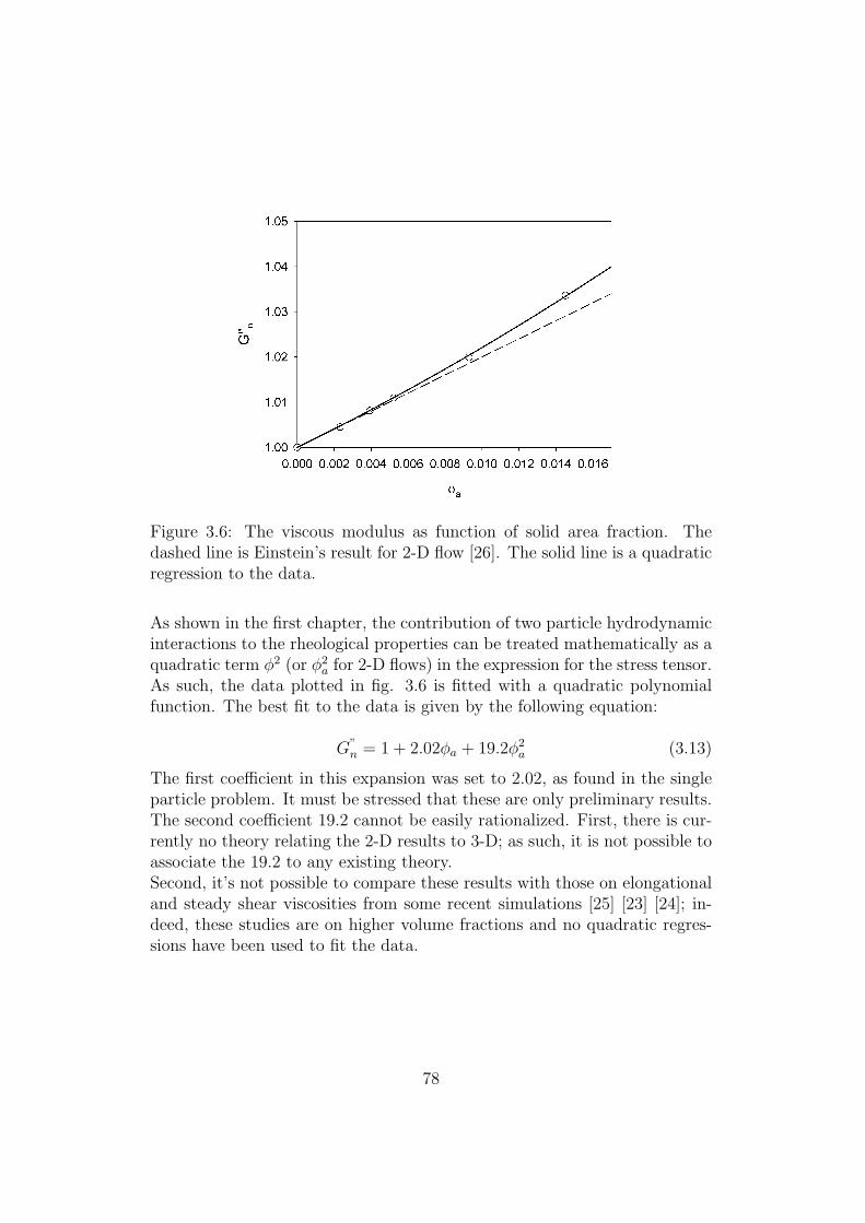
Figure 3.6: The viscous modulus as function of solid area fraction. Thedashed line is Einstein’s result for 2-D flow [26]. The solid line is a quadraticregression to the data.

As shown in the first chapter, the contribution of two particle hydrodynamicinteractions to the rheological properties can be treated mathematically as aquadratic term φ2 (or φ2

a for 2-D flows) in the expression for the stress tensor.As such, the data plotted in fig. 3.6 is fitted with a quadratic polynomialfunction. The best fit to the data is given by the following equation:

G”n = 1 + 2.02φa + 19.2φ2

a (3.13)

The first coefficient in this expansion was set to 2.02, as found in the singleparticle problem. It must be stressed that these are only preliminary results.The second coefficient 19.2 cannot be easily rationalized. First, there is cur-rently no theory relating the 2-D results to 3-D; as such, it is not possible toassociate the 19.2 to any existing theory.Second, it’s not possible to compare these results with those on elongationaland steady shear viscosities from some recent simulations [25] [23] [24]; in-deed, these studies are on higher volume fractions and no quadratic regres-sions have been used to fit the data.

78

3.5 Conclusions

In this chapter, simulations for non Brownian hard disks dispersed in a New-tonian fluid under oscillatory shear flow in a well defined domain were pre-sented. As far as we know, there are currently no simulations that investigatethe dependence of the viscoelastic moduli on volume fraction.We investigated the case of a single particle and of two particles. The stresstensor was calculated in both cases.We focused on the dependence of the viscous modulus on solid area fraction.For the single particle problem, the viscous modulus approaches Einstein′sanalytical solution for 2D [26], showing the feasibility of our scheme.For the two particle problem, the contribution of the hydrodynamic interac-tions to the rheological properties was treated mathematically as a quadraticterm φ2 in the polynomial expansion of the viscous modulus. We found thatthe coefficient is equal to 19. At this moment, this value cannot be easily ra-tionalized: there is no theory relating the 2-D results to 3-D and the existingnumerical results on elongational and steady shear viscosities are for higherconcentrations.

79

Chapter 4

Flow-induced structureformation of spheres inviscoelastic fluids

This chapter focuses on the flow induced microstructure of non-colloidal sus-pensions of spherical particles in viscoelastic fluids. First, the used materialsand methods are presented.Then, the characterization of the suspending fluids, both rheologically andrheo-optically, is shown.In the last part of the chapter, the experimental results are presented and theeffect of the viscoelasticity of the suspending fluid on the structure formationis discussed.

4.1 Materials

4.1.1 Polystyrene particles

Monodisperse polystyrene (PS) spheres have been used as the dispersedphase. The polystyrene particles were found to behave as hard spheres in di-lute suspensions [89]. They were synthesized by a dispersion polymerisationprocess, similar to the one described by Almog et al. [90]. The method is adispersion polymerisation process in an organic phase. The synthesis relies onthe differences in the solubility of styrene and polystyrene in ethanol: styreneis soluble in anhydrous ethanol whereas high molecular weight polystyreneis not. The method depends on incipient aggregation that takes place atthe very early stages of the polymerisation. This determines the numberof formed nuclei. When a critical value molecular weight is reached, short

80

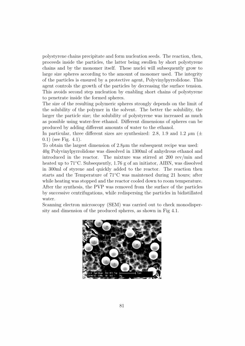
polystyrene chains precipitate and form nucleation seeds. The reaction, then,proceeds inside the particles, the latter being swollen by short polystyrenechains and by the monomer itself. These nuclei will subsequently grow tolarge size spheres according to the amount of monomer used. The integrityof the particles is ensured by a protective agent, Polyvinylpyrrolidone. Thisagent controls the growth of the particles by decreasing the surface tension.This avoids second step nucleation by enabling short chains of polystyreneto penetrate inside the formed spheres.The size of the resulting polymeric spheres strongly depends on the limit ofthe solubility of the polymer in the solvent. The better the solubility, thelarger the particle size; the solubility of polystyrene was increased as muchas possible using water-free ethanol. Different dimensions of spheres can beproduced by adding different amounts of water to the ethanol.In particular, three different sizes are synthesized: 2.8, 1.9 and 1.2 µm (±0.1) (see Fig. 4.1).To obtain the largest dimension of 2.8µm the subsequent recipe was used:40g Polyvinylpyrrolidone was dissolved in 1300ml of anhydrous ethanol andintroduced in the reactor. The mixture was stirred at 200 rev/min andheated up to 71C. Subsequently, 1.76 g of an initiator, AIBN, was dissolvedin 300ml of styrene and quickly added to the reactor. The reaction thenstarts and the Temperature of 71C was maintened during 21 hours; afterwhile heating was stopped and the reactor cooled down to room temperature.After the synthesis, the PVP was removed from the surface of the particlesby successive centrifugations, while redispersing the particles in bidistillatedwater.Scanning electron microscopy (SEM) was carried out to check monodisper-sity and dimension of the produced spheres, as shown in Fig 4.1.

81

Figure 4.1: SEM micrographs of Polystyrene spheres. From the top to thebottom, 2.8 µm, 1.9 µm and 1.2 µm respectively.

The density of particles was measured to be about 1050 Kg/m3 [91].Suspensions containing a volume fraction of 0.008 have been prepared.Charged polysterene particles of 1.6 µm were also used in order to check theimportance of charges in string formation.For the counterrotating rheometer with microscopy devices, PMMA particles(see chapter II) have been used.

4.1.2 Polymer solutions

The suspending fluids were selected to be able to investigate the effects ofviscoelasticity and shear thinning on the particle microstructure under shearflow. Aqueous solutions of hydroxypropylcellulose and polyoxyethyleneoxidewere prepared by adding the right amount of polymer to a suspensions of PSparticles in water. the molecular weights of the polymers and an overwiewof the composition of the suspending fluids are given in tab. 4.1.The densities of the suspending media are about 1100 kg/m3. The small den-sity mismatch between suspending media will not give rise to sedimentationeffects on the time scale of experiments. In particular, using Stokes law, thesedimentation time for polystyrene particles over 10% of the gap for a gap

82

Table 4.1: Molecular weights of the polymers and composition of the sus-pending media.

Polymer Molecular weight (Dalton) %w/wHPC (Klucel LF Hercules) 9500 30%

PEO (Union Carbide) 4 · 106 3%

of h=100 µm can be calculated as follows:

t0.1h =0.45η0h

(ρp − ρ0)R2g(4.1)

with g the acceleration gravity, ρ0 and η0 the density and the viscosity forthe pure suspending medium, R the particle radius and ρp the density of theparticles. In all cases, t0.1h > 3000h.In the performed experiments, the effects of particle inertia can be neglected.In laminar shear flow, the particle Reynolds number is defined as:

Rep =ρ0R

2γ

η0

(4.2)

The Rep value is always smaller than 10−10 in the shear rate range investi-gated.The particle size is sufficiently large to be able to neglect Brownian forces.Indeed, the Peclet number (eq. 1.19 the ratio between the hydrodynamicforces and Brownian motion) is high enough (104 to 108) to state that thehydrodynamic effects will be dominant over Brownian motion.

4.2 Experimental techniques

Rheological measurements on the unfilled suspending media were carried outon two rheometers, a stress controlled rheometer (Rheometric DSR 200) anda strain controlled rheometer (ARES, Rheometric scientific). In both casescone and plate geometry of 25 mm diameter and a cone angle of 0.1 rad wereused. All measurements were carried out at 20C. Temperature was con-trolled by means of Peltier elements, which guaranteed a thermal stabilitywithin ± 0.1C.

Microscopy and small angle light scattering experiments (SALS) were per-formed on suspensions of PS in the discussed suspending media.

83

A parallel plate flow cell (CSS 450, Linkam) has been used for all the opticalexperiments, enabling views in the velocity vorticity plane.The system is composed of two parallel quartz windows. The bottom win-dow is controlled by a motor. Temperature can be changed from ambienttemperature to about 450C. Observations are made 7.5 mm from the centerof the geometry and the viewing area is 2.5 mm in diameter. The rotationalspeeds vary from 0.0001 to 10 rad/s and it is possible to change the gap from50 to 2500 µm.The optical setup consists of a He/Ne laser with a wavelength λ = 632.8nm;it is followed by a pinhole, the shearing cell, a semi transparent screen and aCCD camera to record the images (see Fig. 4.2).Microscopy images and SALS patterns are collected by means of a digital,progressive scan, high resolution 10-bit CCD camera. The camera was con-nected to a digital frame grabber (CORECO, TCI).In order to check the microstructure during flow, light scattering experi-ments were used. Using an in-house developed software (SALS software,K.U.Leuven) time-resolved images were collected at preset time intervals.The scattering images are later treated with an image processing software,Fit2d. The measurements were performed at 20C (±2C).

Figure 4.2: Schematic diagram of SALS setup

84

Principles of light scattering

Before showing the experimental results, it is important to outline the prin-ciples of light scattering essential to understand SALS experiments.Reviews and books of general applications on scattering methods are avail-able [92] [93] as well as a wide body of literature in which rheology andSALS/SAXS experiments are studied and discussed [94] [95] [96].The basic formalism of small angle scattering is similar for light, neutronsand X-rays. The important difference is in the interaction of the radiationwith the scattering medium. As a result, these scattering techniques are verysimilar and some basic definitions are common to all scattering methods.For SALS, light is scattered from regions or volumes with different refractiveindex within the sample.Fig 4.3 depicts a typical SALS experimental setup.

Figure 4.3: Schematic layout of a SALS setup dipicting the incident andscattered beams, the 2-D detector and the definition of the scattered vector(q).

A He/Ne laser impinges on a sample and the scattered intensity in the for-ward direction is recorded by a two dimensional detector (screen). The trans-mitted primary beam is fully absorbed by the beamstop placed in front ofthe detector. The incident wave vector ki will be deviated by the presence ofparticles with a polar angle α, becoming ks. The scattering at small angles isfully elastic because of the high energy of the radiation, so the magnitudes ofthe incident and scattered wave vectors are equal, |ki| = |ks| = 2π

λ. In SALS

85

experiments the intensity of scattering is usually measured as a function ofthe momentum transfer or scattering vector, q = ks − ki and its magnitude:

q =4π

λsin

α

2(4.3)

where λ is the wavelenght and α is the scattering angle (or polar angle).For a dilute system containing N uniform particles per unit volume, the interparticle interactions can be neglected and I(q,θ), that is the intensity at anyscattered vector and azimuthal angle, mainly depends on the shape and sizeof the particles. It can be calculated by summing the scattered amplitudes,F(q,θ), that arise from all parts of the sample as:

I(q, θ) =∑

F (q, θ)F ∗(q, θ) (4.4)

where the sum is taken over the entire sample and F ∗(q, θ) is the complexconjugate of F(q,θ). If the summation is replaced by an integral, the form ofthe eq. 4.4 closely resembles a Fourier transform of the distribution of scat-teries in the sample. This recognition of the scattered intensity as a Fouriertransform leads to several simplifications in the interpretation of data. Forexample, the convolution theorem allows eq. 4.4, for the case of interactingparticles, to be written as:

I(q, θ) = cP (q, θ)S(q, θ) (4.5)

where P(q) is the form factor of a particle and S(q) is the structure factor,related to the microstructure through the pair correlation function. In otherwords, P(q) is related to the correlation within a single particle and S(q),instead, describes the correlations between different particles.The constant c depends on other characteristics of the suspensions (volumefraction, difference in the refractive indeces,...).The quantity P(q) is calculated for many simple shapes.If the particle in a suspension are solid, P(q) will be constant and any changein scattered intensities during shear will arise from in a change in the mi-crostructure (S(q)). Although eq. 4.5 might suggest that it is easy to extractthe structure factor from measurements of the intensity by calculating theform factor, in practice several difficulties are not easily resolvable (discussedin more detail elsewhere [97]).Anyway, the study of the intensity can be useful to understand microstruc-tural changes. The two-dimensional SALS patterns provide informationabout the suspensions microstructure in reciprocal space. Fig. 4.4 showson the left a schematic diagram of the anisotropic structure before shearing

86

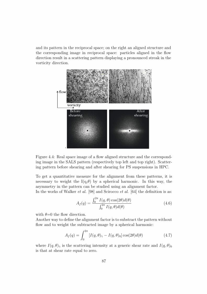
and its pattern in the reciprocal space; on the right an aligned structure andthe corresponding image in reciprocal space: particles aligned in the flowdirection result in a scattering pattern displaying a pronounced streak in thevorticity direction.

Figure 4.4: Real space image of a flow aligned structure and the correspond-ing image in the SALS pattern (respectively top left and top right). Scatter-ing pattern before shearing and after shearing for PS suspensions in HPC.

To get a quantitative measure for the alignment from these patterns, it isnecessary to weight the I(q,θ) by a spherical harmonic. In this way, theasymmetry in the pattern can be studied using an alignment factor.In the works of Walker et al. [98] and Scirocco et al. [64] the definition is as:

Af (q) =

∫ 2π

0I(q, θ) cos(2θ)d(θ)∫ 2π

0I(q, θ)d(θ)

(4.6)

with θ=0 the flow direction.Another way to define the alignment factor is to substract the pattern withoutflow and to weight the subtracted image by a spherical harmonic:

Af (q) =

∫ 2π

0

[I(q, θ)γ − I(q, θ)0] cos(2θ)d(θ) (4.7)

where I(q, θ)γ is the scattering intensity at a generic shear rate and I(q, θ)0

is that at shear rate equal to zero.

87

The counterrotating rheometer combined with microscopy

Another device is used to quantify the migration. A special designed coun-terrotating rheometer is combined with an optical microscopy setup, as infig. 4.5. The counterrotating rheometer is composed of two stress controlledrheometers: a Physica MCR-300 for the top geometry, and a Physica DSR-300 for the bottom geometry (Paar Physica, Austria). These rheometers canbe independently controlled.A BK7 glass parallel plate geometry with a plain diameter of 50mm in com-bination with an in-house developed glass cup that surrounds the bottomplate to keep the sample in place is used as flow geometry.Since the rheometer is counter-rotating, there is a stagnation plane with ve-locity zero in between the glass plates. This zero-velocity plane can be shiftedup and down using a potentiometer which adjusts the rotation speed of thebottom and top plate, while keeping the shear rate constant. As such it isreadily possible to capture a particle and keep it in view of the optical setupwhile all effects of the shear flow are working on the particle, although themean particle velocity is zero.The optical setup is composed of a Wild M5A stereomicroscope (Heerbrugg,Switzerland) connected to a Basler A301-fc digital camera (80 frames/s, 8 bit,resolution 658x494, progressive scan). This enables one to record sequencesof images on a computer using Streampix software (Norpix, Canada).A prism in between the microscope and the top parallel plate is used, and,as condenser, a energy saving lamp in conjunction with a small mirror. Thissetup enables one to record images of strings in the zero shear velocity plane.A schematic representation of the counterrotating Physica and the opticalsetup is shown in fig. 4.5To locate the radial position of the particle in the geometry (to be able to geta value for the shear rate on the particle) we look with the microscope at aplastic ”grid”, which is placed between the cup and the bottom plate. Usingthis method one can measure the radial position of the particle in the geom-etry with an accuracy better then 200µm, with an error on the shear rateof about 1%. All measurements on the particles are done at radial positionsbetween 15 and 19mm, the first limit is due to the geometry itself which isopaque in the middle, the upper one comes from the quality of the flow field.Usually, the gap is about 500 µm; at smaller gaps a small misalignment ofthe parallel plates affects the measurements. Higher gaps don’t allow a goodstudy of the migration phenomenon. Only one shear rate of 10s−1 has beenstudied.

88

Figure 4.5: The counterrotating rheometer combined with microscopy from[55].

The recorded sequences of pictures were analyzed using Streampix and Im-ageJ software [99].

89

4.3 Experimental results

4.3.1 Rheology of suspending fluids

The steady state material functions for the HPC and PEO suspending mediaare presented in figs. 4.6 and 4.7.

Figure 4.6: Viscosity of the fluids as function of shear rate.

Figure 4.7: First normal stress coefficients of the fluids as function of shearrate.

90

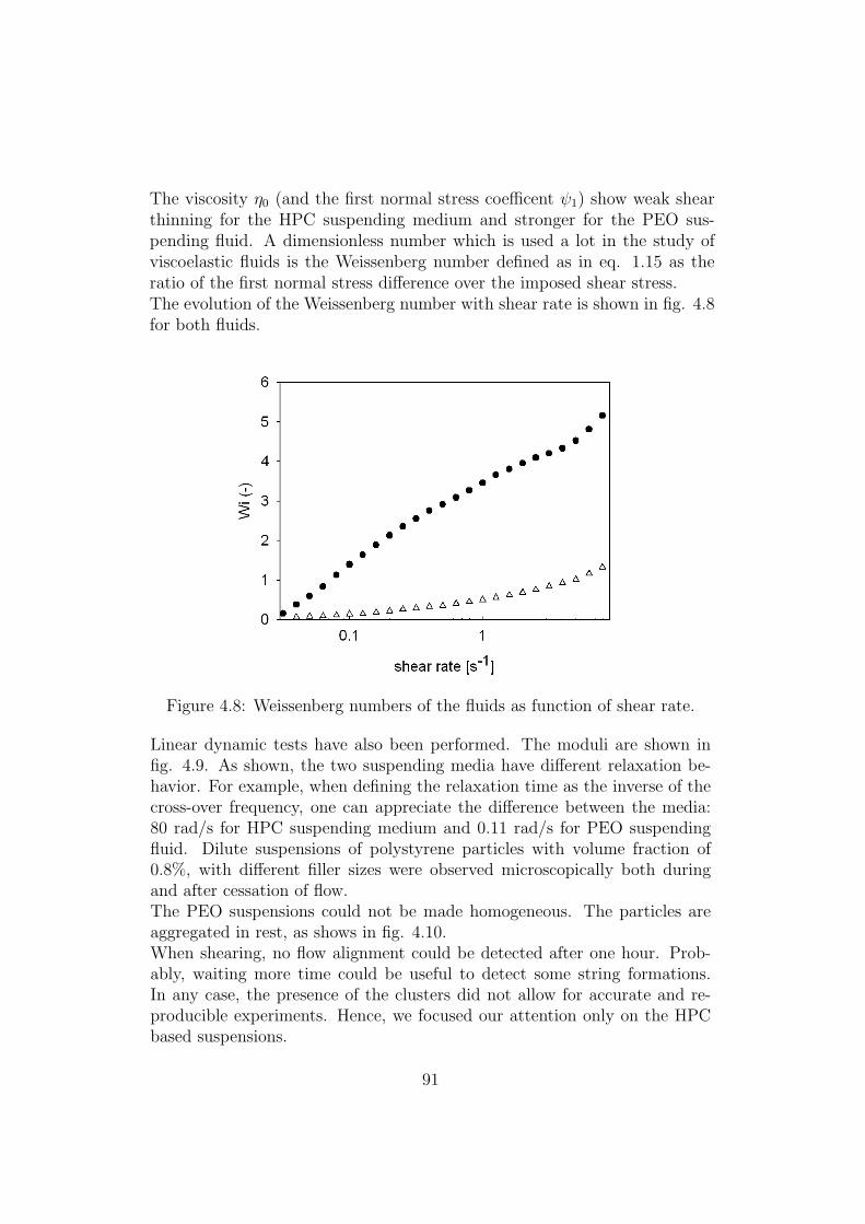
The viscosity η0 (and the first normal stress coefficent ψ1) show weak shearthinning for the HPC suspending medium and stronger for the PEO sus-pending fluid. A dimensionless number which is used a lot in the study ofviscoelastic fluids is the Weissenberg number defined as in eq. 1.15 as theratio of the first normal stress difference over the imposed shear stress.The evolution of the Weissenberg number with shear rate is shown in fig. 4.8for both fluids.

Figure 4.8: Weissenberg numbers of the fluids as function of shear rate.

Linear dynamic tests have also been performed. The moduli are shown infig. 4.9. As shown, the two suspending media have different relaxation be-havior. For example, when defining the relaxation time as the inverse of thecross-over frequency, one can appreciate the difference between the media:80 rad/s for HPC suspending medium and 0.11 rad/s for PEO suspendingfluid. Dilute suspensions of polystyrene particles with volume fraction of0.8%, with different filler sizes were observed microscopically both duringand after cessation of flow.The PEO suspensions could not be made homogeneous. The particles areaggregated in rest, as shows in fig. 4.10.When shearing, no flow alignment could be detected after one hour. Prob-ably, waiting more time could be useful to detect some string formations.In any case, the presence of the clusters did not allow for accurate and re-producible experiments. Hence, we focused our attention only on the HPCbased suspensions.

91

Figure 4.9: Viscoelastic moduli for the suspending media as function of fre-quency.

Figure 4.10: Microscopy image of PEO’s suspension with 3µm diameterspheres.

4.3.2 Microscopy

The particles in the HPC suspensions were initially randomly dispersed. Dif-ferences in the microstructure have been studied for different particle sizes.Dilute suspensions, φ=0.8%, of polystyrene particles( with diameters 2.8µm,1.9µm, 1.2µm ±0.1), were sheared and observed microscopically both duringflow and after cessation of flow.When shearing the suspensions for a sufficiently long time, string-like struc-tures were observed to develop. Differences and similarities can be studiedfor the different particle sizes.

92

In all cases, alignment and migration were coupled: first migration towardsthe plates took place, then the particles aligned. Alignment in the bulk ofthe fluid was never detected.

Migration effects, as clearly demonstrated before (see first chapter), are pro-moted by the fluid normal stress difference and shear thinning.Migration and the consequent alignment are stronger when the shear rate isincreased.To examine the relation between migration velocity and the normal stresses,it is possible to write a simple force balance for a neutrally buoyant particle,following the work of Tehrani et al [77]:

6πRη0vz ∝ R3N1 −N2

z(4.8)

where z is the coordinate in the vorticity direction, R the particle radius,vz the velocity of the migration towards the walls and N1 and N2 the firstand second normal stress differences. Neglecting N2, the equation can bere-written in terms of the migration velocity:

vz ∝ N1R2

6πη0z(4.9)

Using η0 = σγ

for the viscosity and N1

σfor the Weissenberg number, one

obtains:

vz ∝ WiγR2

6πz(4.10)

According to eq. 4.10, the migration velocity is proportional to the square ofthe particle and to the product of the Weissenberg number and shear rate.Increasing the gap results (not so clear because of the turbidity of the sam-ple) in less alignment of the particles at the plate compared to the smallergaps for the same shear rates. In any case, alignment in the bulk was neverobserved (see fig. 4.11).Another possibility is to increase the volume fraction: probably the align-

ment is due only to a local increase of the volume fraction on the wall; theincreasing of the volume fraction could bring to stronger hydrodynamic inter-actions between particles that could definitively ”win” the migration forcestowards the walls and align in the bulk.Also this hypothesis does not give any result: particles go towards the wallmore easily with increasing volume fraction [100] and inside the bulk anystring formation in the direction of the flow was not detected.The evolution of the microstructure under shear for particles of 3 µm is shownin fig. 4.12. The top left picture is the microstructure at shear rate zero.

93

Figure 4.11: Microscopy images of a HPC suspension at 30s−1 and 200µmgap (diameter spheres=1.9 µm). After 1h: on the left side the microstructureon the plate; on the right side in the bulk.

The right top picture is after shearing the suspension for one hour at 30s−1.The bottom picture is, finally, the bulk after shearing: no alignment couldbe detected inside the sample. One can clearly see that the concentrationin the bulk is lower than on the plates, this because the particles migratedtowards the plates.

Figure 4.12: Microscopy image of a HPC suspension at 30s−1, 100µm gap(diameter spheres=3µm). Top left: before shearing. Top right: on the plateafter shearing 1h. Bottom: in the bulk after shearing 1h.

The time for forming the strings decreases with increasing shear rate. For

94

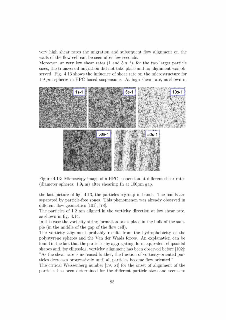
very high shear rates the migration and subsequent flow alignment on thewalls of the flow cell can be seen after few seconds.Moreover, at very low shear rates (1 and 5 s−1), for the two larger particlesizes, the transversal migration did not take place and no alignment was ob-served. Fig. 4.13 shows the influence of shear rate on the microstructure for1.9 µm spheres in HPC based suspensions. At high shear rate, as shown in

Figure 4.13: Microscopy image of a HPC suspension at different shear rates(diameter spheres: 1.9µm) after shearing 1h at 100µm gap.

the last picture of fig. 4.13, the particles regroup in bands. The bands areseparated by particle-free zones. This phenomenon was already observed indifferent flow geometries [101], [78].The particles of 1.2 µm aligned in the vorticity direction at low shear rate,as shown in fig. 4.14.In this case the vorticity string formation takes place in the bulk of the sam-ple (in the middle of the gap of the flow cell).The vorticity alignment probably results from the hydrophobicity of thepolystyrene spheres and the Van der Waals forces. An explanation can befound in the fact that the particles, by aggregating, form equivalent ellipsoidalshapes and, for ellipsoids, vorticity alignment has been observed before [102]:”As the shear rate is increased further, the fraction of vorticity-oriented par-ticles decreases progressively until all particles become flow oriented.”The critical Weissenberg number [59, 64] for the onset of alignment of theparticles has been determined for the different particle sizes and seems to

95

Figure 4.14: Microscopic image of HPC suspension with 1.2µm spheres inthe bulk of the liquid after shearing at 1 s−1.

be nearby independent on particle size. It can be said that 0.5 < Wicr < 1for this fluid, where the first number refers to high shear rates at which noalignment could be detected, whereas the second one corresponds to the nextshear rate, at which alignment could be seen. We consider a string as a struc-ture with at least three particles, chained and aligned in the flow direction.The Weissenberg number and the onset of flow alignment (at the walls) cor-responding to various shear rates are determined by microscopy and shownin table 4.2.

Table 4.2: Weissenberg number and onset of alignment as function of shearrate.

shearrate flowalignment? Wi1 no 0.55 yes 110 yes 1.3530 yes 1.550 yes 1.6

The last two values of the Weissenberg number are extrapolated from theplot in fig. 4.8.

96

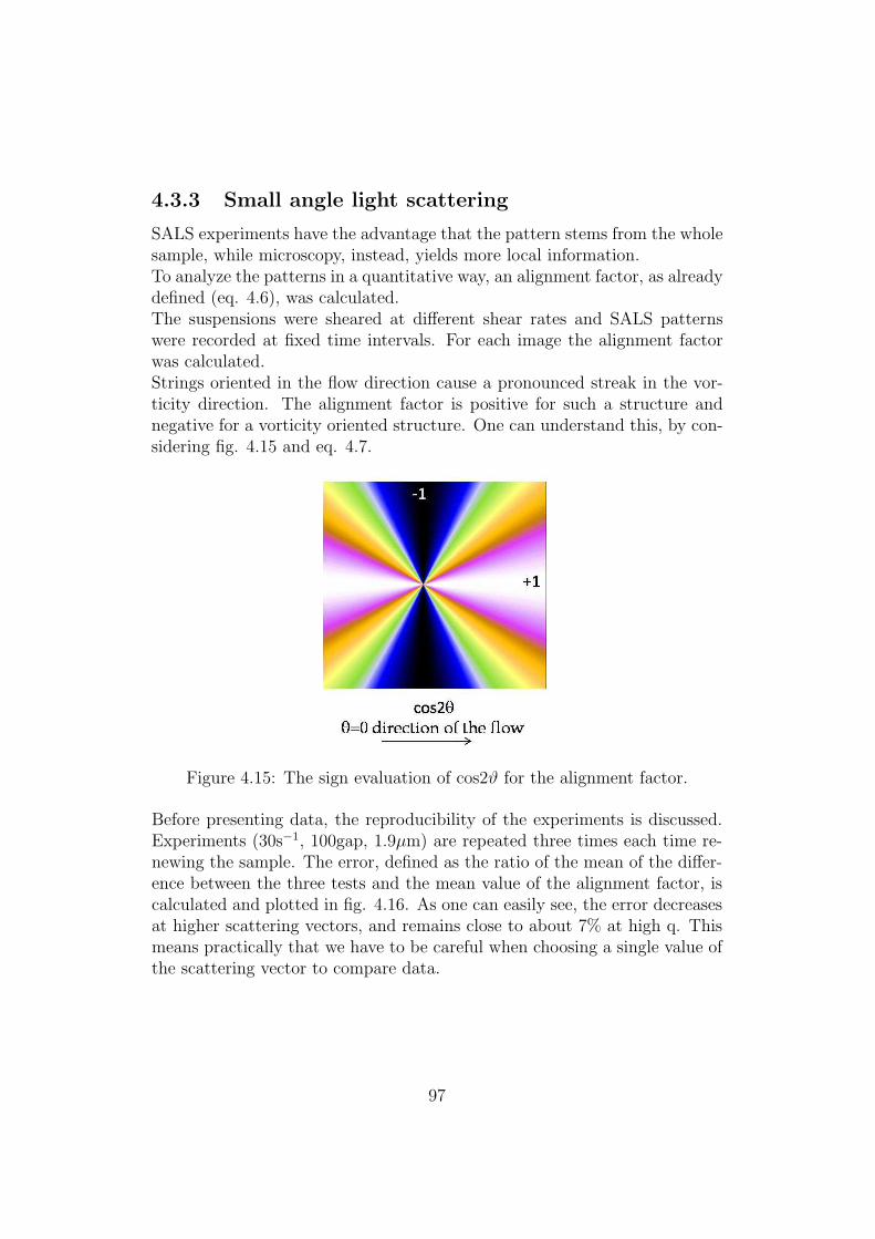
4.3.3 Small angle light scattering

SALS experiments have the advantage that the pattern stems from the wholesample, while microscopy, instead, yields more local information.To analyze the patterns in a quantitative way, an alignment factor, as alreadydefined (eq. 4.6), was calculated.The suspensions were sheared at different shear rates and SALS patternswere recorded at fixed time intervals. For each image the alignment factorwas calculated.Strings oriented in the flow direction cause a pronounced streak in the vor-ticity direction. The alignment factor is positive for such a structure andnegative for a vorticity oriented structure. One can understand this, by con-sidering fig. 4.15 and eq. 4.7.

Figure 4.15: The sign evaluation of cos2ϑ for the alignment factor.

Before presenting data, the reproducibility of the experiments is discussed.Experiments (30s−1, 100gap, 1.9µm) are repeated three times each time re-newing the sample. The error, defined as the ratio of the mean of the differ-ence between the three tests and the mean value of the alignment factor, iscalculated and plotted in fig. 4.16. As one can easily see, the error decreasesat higher scattering vectors, and remains close to about 7% at high q. Thismeans practically that we have to be careful when choosing a single value ofthe scattering vector to compare data.

97

Figure 4.16: Evaluation of percent error in a meaningful q range for 1.9 µmbased suspension.

Alignment factor dependence on shear rate

Under steady state conditions the patterns change with shear rate as shownin fig. 4.17. At first stage, we use eq. 4.7 to calculate Af .

Figure 4.17: SALS patterns as function of shear rate for 1.2 µm size particle.At low shear rates, a weak vorticity alignment can be see. Increasing theshear rate reorients the strings in the flow direction.

In order to understand the evolution of the alignment factor as a function ofshear rate, it is necessary to compare the patterns at the same deformation(γ = γ∆t) or at the same time. The results for the 1.2 µm size suspensionsare shown in figs 4.18 and 4.19. The behavior is however qualitatively thesame for all sizes (except for the vorticity alignment phenomenon at lower

98

shear rates).In Fig. 4.18, the alignment factor as function of the scattering vector isshown for different shear rates at fixed deformation. We are not able to showthe lowest shear rates, for which such a high deformation was not reached inour experiments.

Figure 4.18: Alignment factor as function of scattering vector at 360% strainfor the 1.2 µm size suspension.

Another way to compare the data of different shear rates is at the sameshearing time; the result is shown in fig. 4.19. In this case it is possible tocompare the alignment factor for all experimental shear rates.

99

Figure 4.19: Alignment factor as function of scattering vector after 1h for1.2 µm size spheres.

It is clear from figs. 4.18 and 4.19 that, at a fixed q, or for a range of qvalues, the alignment factor increases with increasing shear rate.For the 1.2 µm spheres the alignment factor observed under steady stateconditions for a fixed scattering vector q=1[µm−1] is plotted in Fig. 4.20.The alignment factor is negative, indicating vorticity alignment, for shearrate below 10s−1.

Figure 4.20: Alignment factor as function of shear rate at a scattering vectorof 1µm−1.

100

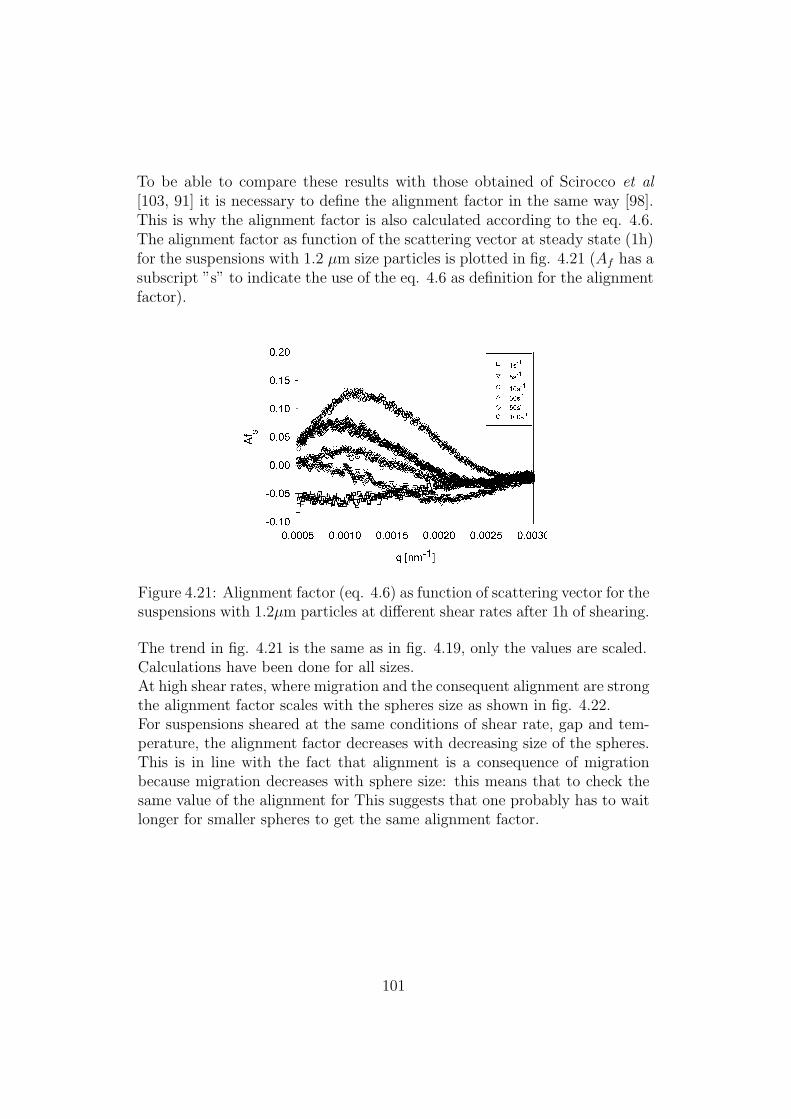
To be able to compare these results with those obtained of Scirocco et al[103, 91] it is necessary to define the alignment factor in the same way [98].This is why the alignment factor is also calculated according to the eq. 4.6.The alignment factor as function of the scattering vector at steady state (1h)for the suspensions with 1.2 µm size particles is plotted in fig. 4.21 (Af has asubscript ”s” to indicate the use of the eq. 4.6 as definition for the alignmentfactor).

Figure 4.21: Alignment factor (eq. 4.6) as function of scattering vector for thesuspensions with 1.2µm particles at different shear rates after 1h of shearing.

The trend in fig. 4.21 is the same as in fig. 4.19, only the values are scaled.Calculations have been done for all sizes.At high shear rates, where migration and the consequent alignment are strongthe alignment factor scales with the spheres size as shown in fig. 4.22.For suspensions sheared at the same conditions of shear rate, gap and tem-perature, the alignment factor decreases with decreasing size of the spheres.This is in line with the fact that alignment is a consequence of migrationbecause migration decreases with sphere size: this means that to check thesame value of the alignment for This suggests that one probably has to waitlonger for smaller spheres to get the same alignment factor.

101

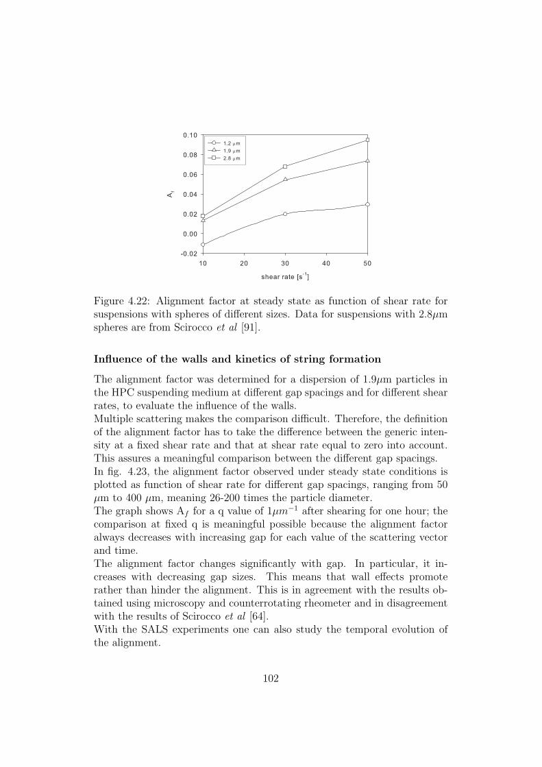
Figure 4.22: Alignment factor at steady state as function of shear rate forsuspensions with spheres of different sizes. Data for suspensions with 2.8µmspheres are from Scirocco et al [91].

Influence of the walls and kinetics of string formation

The alignment factor was determined for a dispersion of 1.9µm particles inthe HPC suspending medium at different gap spacings and for different shearrates, to evaluate the influence of the walls.Multiple scattering makes the comparison difficult. Therefore, the definitionof the alignment factor has to take the difference between the generic inten-sity at a fixed shear rate and that at shear rate equal to zero into account.This assures a meaningful comparison between the different gap spacings.In fig. 4.23, the alignment factor observed under steady state conditions isplotted as function of shear rate for different gap spacings, ranging from 50µm to 400 µm, meaning 26-200 times the particle diameter.The graph shows Af for a q value of 1µm−1 after shearing for one hour; thecomparison at fixed q is meaningful possible because the alignment factoralways decreases with increasing gap for each value of the scattering vectorand time.The alignment factor changes significantly with gap. In particular, it in-creases with decreasing gap sizes. This means that wall effects promoterather than hinder the alignment. This is in agreement with the results ob-tained using microscopy and counterrotating rheometer and in disagreementwith the results of Scirocco et al [64].With the SALS experiments one can also study the temporal evolution ofthe alignment.

102

Figure 4.23: Effect of the gap width on the alignment factor for a dispersionof 1.9µm spheres in the HPC based suspending medium. Steady state atq=1µm−1.

In fig. 4.24, the alignment factor is plotted as a function of time for differentgaps for a shear rate of 30s−1.The kinetics of string formation are different for different gaps; for the small-est gap, there are two things to look at: the smaller number of the particlesthat have to align and the smaller distance between the particle in the bulkand the plate of the flow cell. The result is in an alignment that saturatesvery fast, meaning that the plateau is easily reached.The first derivative of the alignment factor can be calculated from fig. 4.24and, at least in first approximation, is a measure of migration. At start of theflow, the alignment is mainly dependent on migration. The first derivativeis shown in fig. 4.25 as function of gap. According to eq. 4.10:

vz ∝ dAf

dt∝ 1

gap(4.11)

the migration velocity depends hyperbolically on gap, as clearly shown in fig.4.25.To understand the role of the shearing time on the migration and, hence, thealignment, an experiment is performed at 30s−1 for about three hours, thelimit being imposed by the device. To avoid confusion, in fig. 4.26 the resultis shown for a mean of the alignment factor in a certain scattering vectorrange (3*10−4-2*10−3nm−1); therefore, it is not possible to directly comparethese values with data in fig. 4.24 at the same gap.

103

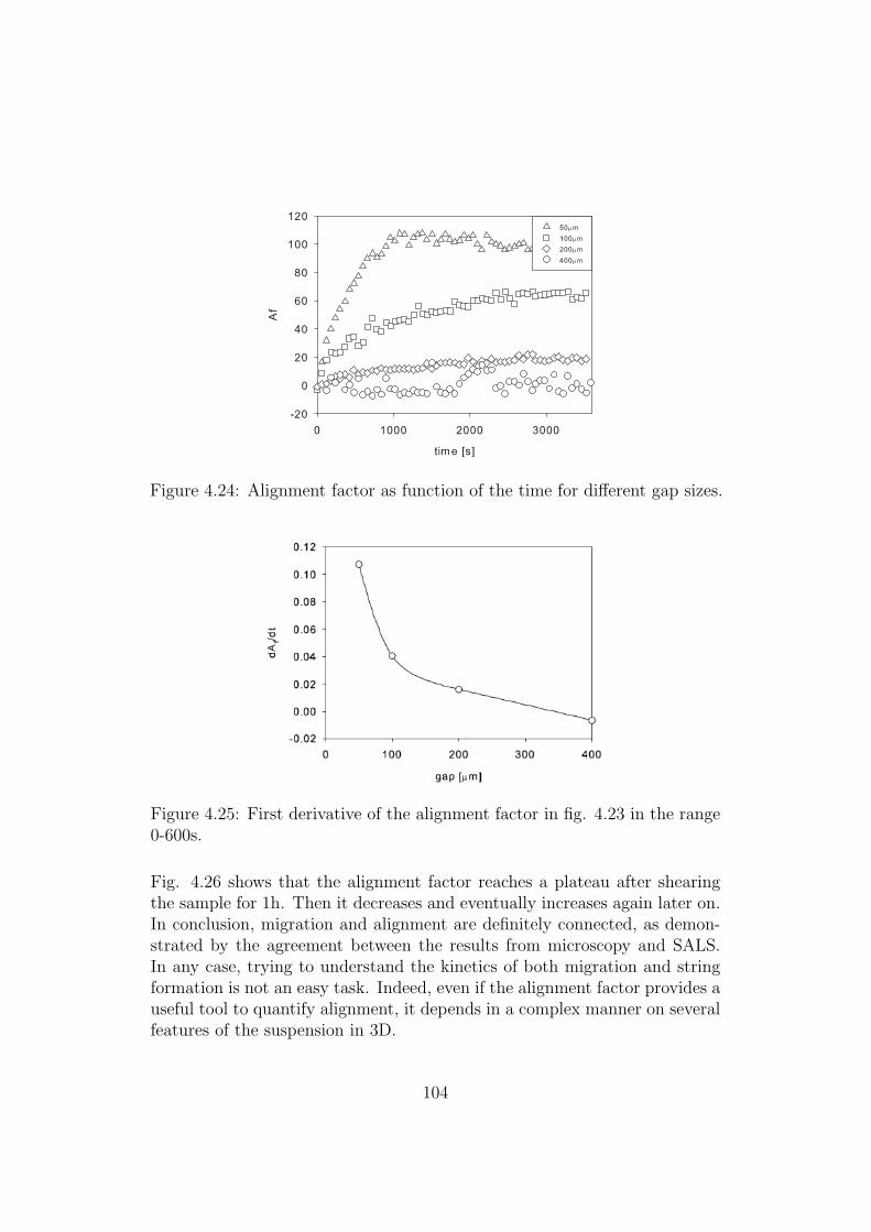
Figure 4.24: Alignment factor as function of the time for different gap sizes.

Figure 4.25: First derivative of the alignment factor in fig. 4.23 in the range0-600s.

Fig. 4.26 shows that the alignment factor reaches a plateau after shearingthe sample for 1h. Then it decreases and eventually increases again later on.In conclusion, migration and alignment are definitely connected, as demon-strated by the agreement between the results from microscopy and SALS.In any case, trying to understand the kinetics of both migration and stringformation is not an easy task. Indeed, even if the alignment factor provides auseful tool to quantify alignment, it depends in a complex manner on severalfeatures of the suspension in 3D.

104

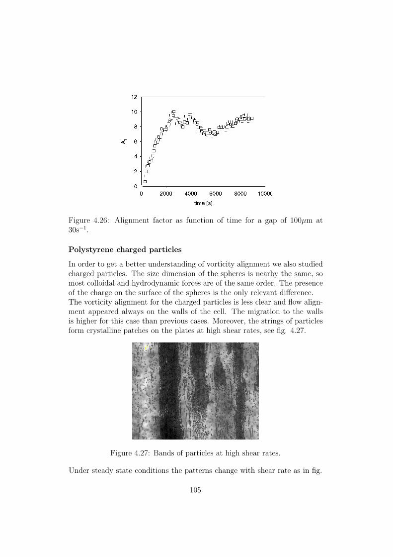
Figure 4.26: Alignment factor as function of time for a gap of 100µm at30s−1.

Polystyrene charged particles

In order to get a better understanding of vorticity alignment we also studiedcharged particles. The size dimension of the spheres is nearby the same, somost colloidal and hydrodynamic forces are of the same order. The presenceof the charge on the surface of the spheres is the only relevant difference.The vorticity alignment for the charged particles is less clear and flow align-ment appeared always on the walls of the cell. The migration to the wallsis higher for this case than previous cases. Moreover, the strings of particlesform crystalline patches on the plates at high shear rates, see fig. 4.27.

Figure 4.27: Bands of particles at high shear rates.

Under steady state conditions the patterns change with shear rate as in fig.

105

4.28. As said before, except weakly for the shear rate of 1s−1, vorticityalignment is not observed.

Figure 4.28: SALS patterns as function of shear rate for 1.6 µm size chargedparticle.

106

4.3.4 Counterrotating device

The velocity of a particle in a string can be determined taking into consider-ation the ratio pixel/µm (=0.63 for an image of 654×494 and magnificationof 50×) and the time for a particle in a string to travel the length of theimage. As the shear rate on the particle and the position of the zero-velocityplane are known, it is possible to calculate the position of the particle withrespect to the position of the plates.To get an accurate measurement of the velocity of the particle in a string,many particles were considered, both of the bottom and of the top plate.The final velocity is an average of all velocities calculated.In this device, different suspending media filled with PMMA particles of15µm diameter (0.8% by volume) were used: Newtonian PIB, as a reference,and a shear thinning elastic polymer solution of HPC in water (used beforein all the other experiments).

First of all, the Newtonian based suspension was checked and string forma-tion was found to be absent. This agrees with the hypothesis that migrationand alignment are strictly connected. Migration is absent in the Newtonianfluid [103, 59], at least when inertia can be neglected, as in this case; con-sequently the string formation cannot take place. This is, of course, not theonly reason why alignment is absent in the Newtonian fluid: alignment isalso connected to time effects of the fluid and to the non-symmetric natureof the hydrodynamic interactions in viscoelastic fluids.

Then, the HPC based suspensions were studied (Fig 4.29). Even if the mi-gration and the alignment on the walls of the flow cell have been alreadystudied optically, the counterrotating device is very useful, as said before,to check the distance of the strings from the plates. In particular, it wascalculated that the distance of the center of the sphere in a string from boththe plates was about 5µm...that’s impossible for the PMMA particles whichhave 15µm as mean diameter! This means that, considering the sum of theerrors for the measuring of all the measurements, the particles are sticky tothe plates and align on the plate itself.

107

Figure 4.29: Counterrotating image for HPC based suspensions.

4.4 Conclusions

The effect of particle size and presence of the wall on flow alignment havebeen studied in HPC based suspensions, by means of video microscopy andwith small angle light scattering. Alignment factor were derived from theSALS patterns.The critical Weissenberg number for the onset of alignment found using mi-croscopy is indipendent of particle size. A new phenomenon was found forour smallest spheres: a vorticity aligned structure was observed at low shearrates, never seen before for spherical particles [103, 65]. This probably comesfrom a competition between different forces, hydrodynamic interactions, col-loidal forces (such as Van der Waals forces) etc. Decreasing the diameterof the spheres results in more particles and more surface area at a certainvolume fraction. This could explain, together with the hydrophobicity of thepolystyrene spheres, the vorticity alignment: at low shear rates, the spheresaggregate and form ellipsoidal shapes; the number of strings oriented in thevorticity direction increases with longer shearing. Moreover, as the shearrate is increased further, the fraction of vorticity-oriented particles decreasesprogressively until all particles migrate to the walls and flow orient. Thisphenomenon for non-spherical particles has been studied before [102] [104].With SALS, we found that the alignment factor increases with particle size.The best way to compare the alignment factors for different particle sizes isto average its values for a range of scattering vectors: 0.9q∗ < q < 1.1q∗,where q∗ is the scattering vector value corresponding to a real space distanceof five times the particle radius R (q∗5R = π). Fig. 4.30 shows the alignmentfactor at steady state as function of shear rate for different particle sizes.

108

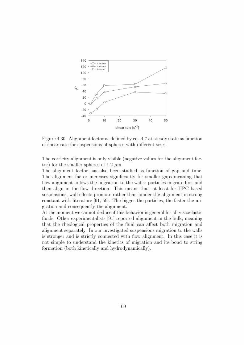
Figure 4.30: Alignment factor as defined by eq. 4.7 at steady state as functionof shear rate for suspensions of spheres with different sizes.

The vorticity alignment is only visible (negative values for the alignment fac-tor) for the smaller spheres of 1.2 µm.The alignment factor has also been studied as function of gap and time.The alignment factor increases significantly for smaller gaps meaning thatflow alignment follows the migration to the walls: particles migrate first andthen align in the flow direction. This means that, at least for HPC basedsuspensions, wall effects promote rather than hinder the alignment in strongconstant with literature [91, 59]. The bigger the particles, the faster the mi-gration and consequently the alignment.At the moment we cannot deduce if this behavior is general for all viscoelasticfluids. Other experimentalists [91] reported alignment in the bulk, meaningthat the rheological properties of the fluid can affect both migration andalignment separately. In our investigated suspensions migration to the wallsis stronger and is strictly connected with flow alignment. In this case it isnot simple to understand the kinetics of migration and its bond to stringformation (both kinetically and hydrodynamically).

109

List of publications

Publication in International Journals

• R. Pasquino, N. Grizzuti, P.L. Maffettone, F. Greco, Rheology of di-lute and semi-dilute non colloidal hard sphere suspensions, Journal ofRheology, 52(6), 1369-1384 (2008).

• S. Acierno, R. Pasquino, N. Grizzuti, Rheological techniques for the de-termination of the crystallization kinetics of a rubber filled polypropy-lene, Journal of Thermal Analysis and Calorimetry, JTAC Special Issue”Rheology as Thermoanalytical Method for Polymers”, (2008)

Congress Contributions

• C. Carotenuto, N. Grizzuti, R.Pasquino, Phase transition of cellulosicbiopolymer solutions, 77th Annual Meeting of Rheology, Vancouver,Canada (2005).

• R. Pasquino, N. Grizzuti, P. L. Maffettone, F. Greco, Rheology of diluteviscoelastic suspensions, 4th Annual European Rheology Conference,Naples, Italy, (2007).

• R. Pasquino, N. Grizzuti, P. L. Maffettone, F. Greco, Rheology of di-lute viscoelastic suspensions, European Polymer Congress, Portoroz,Slovenia, (2007).

• R. Pasquino, N. Grizzuti, P. L. Maffettone, F. Greco, Reologia disospensioni viscoelastiche, INSTM, Perugia, Italy, (2007).

• N. Grizzuti, R. Pasquino, Effects of matrix viscoelasticity on the rhe-ology of dilute and semi dilute suspensions of non Brownian rigidspheres, XVth International Congress on Rheology, Monterey, Cali-fornia, (2008).

110

Curriculum vitae

Rossana Pasquino was born in 1982, Avellino, Italy.In 2000 she got her scientific diploma (Benevento, G. Rummo).She studied Chemical Engineering at University Federico II, Naples, whereshe obtained a degree cum laude in 2005; the thesis was performed in rheol-ogy of biopolymer solutions and in their phase transitions by heating.In November 2005 she started a Ph.D. at the laboratory of the Department ofchemical engineering in the University Federico II in Naples. In August 2007she moved to Belgium to do a part of the Ph.D. project at the Laboratoryof Applied Rheology, K.U. Leuven.

111

Bibliography

[1] Eirich, Bunzle, and Margaretha. The viscosity of suspensions and solu-tions; the viscosity of suspensions of spheres. Kolloid Z, 74:276, 1936.

[2] A. Einstein. Berichtigung zu Meiner Arbeiten: Eine Neue Bestimmungder Molekul Dimensionen. Annalen der Physik Berlin, 34:591, 1911.

[3] O. Bachle. The viscosity of latex and latex mixtures. Rubber Chem.Tech., 10:675, 1937.

[4] C.M. Blow. The viscosity of rubber solution. Trans. Faraday Soc.,25:458, 1929.

[5] G.K. Batchelor and J.T. Green. The determination of the bulk stress ina suspension of spherical particles to order c2. J. Fluid Mech., 56:401,1972.

[6] G.K. Batchelor and J.T. Green. The hydrodynamic interaction of twosmall freely-moving spheres in a linear flow field. J. Fluid Mech., 56:375,1972.

[7] G.K. Batchelor. The effect of brownian motion on the bulk stress in asuspension of spherical particles. J. Fluid Mech., 83:97, 1977.

[8] W. B. Russel and A. P. Gast. Non equilibrium statistical mechanicsof concentrated colloidal dispersions: Hard spheres in weak flows, vol-ume 84. 1985.

[9] I.R. Rutgers. Relative viscosity of suspensions of rigid spheres in new-tonian liquids. Rheol. Acta, 2:202, 1961.

[10] S. H. Maron. Rheological of synthetic latex. J. Colloid Sci., 10:482,1955.

[11] H. Eilers. The viscosity of emulsions of a highly viscous substance asa function of concentration. Kolloid-Z, 97:313, 1941.

112

[12] J.V. Robinson. The viscosity of dispersions of spheres. iii sedimentvolume as a determining parameter. Trans. Soc. Rheology, 1:15, 1957.

[13] A.P. Ting and R.M. Luebbers. Viscosity of suspensions of sphericaland other isodimensional particles in liquids. Amer. Inst. Chem. Eng.J., 3:111, 1957.

[14] K.H. Sweeney and R.D. Geckler. J. Appl. Phys., 25:1135, 1954.

[15] F.L. Saunders. Rheological properties of monodisperse latex systemsconcentration dependence of relative viscosity. J. Coll. Sci., 16:13,1961.

[16] C.U. Thomas and M. Muthukumar. Three-body hydrodynamic effectson viscosity of suspensions of spheres. J. Chem. Phys., 94:5180, 1991.

[17] C.W.J. Beenakker. The effective viscosity of a concentrated suspensionof spheres (and its relation to diffusion). Physica, 128A:48, 1984.

[18] C.W. Macosko. Rheology: principles, measurements, and applications(Foams, Emulsion and Blends. Wiley-VCH, New York, 1994.

[19] J.M. Krieger and A. Dougherty. A mechanism for non-newtonian flowin suspensions of rigid spheres. Tran. Soc. Rheol., 3:137, 1959.

[20] C.H. Hsueh and P.F. Becher. Effective viscosity of suspensions ofspheres. J. Am. Ceram. Soc., 88:1046, 2005.

[21] J. G. Oldroyd. The elastic and viscous properties of emulsions andsuspensions. Proc. R. Soc. London, 218:122, 1953.

[22] S. J Choi and W. R Schowalter Rheological properties of non-dilutesuspensions of deformable particles. Physics of fluids, 18:420, 1975.

[23] W.R. Hwang M.A. Hulsen and H.E.H. Meijer. Direct simulation ofparticle suspensions in sliding bi-periodic frames. J. Comput. Phys.,194:742, 2003.

[24] W.R. Hwang and M.A. Hulsen. Toward the computation rheometry offilled polymeric fluids. Korea-Australia Rheol.J., 18:171, 2006.

[25] G. DAvino, P.L. Maffettone M.A. Hulsen and G.W.M. Peters. A nu-merical method for simulating concentrated rigid particle suspensionsin an elongational flow using a fixed grid.

113

[26] J.F. Brady. The einstein viscosity correction in n-dimensions. Int. J.Multiphase Flow, 10:113, 1984.

[27] G.J. Jarzebsky. On the effective viscosity of pseudoplastic suspensions.Rheol. Acta, 20:280, 1981.

[28] Donald L. Koch and G. Subramanian. The stress in a dilute suspensionof spheres suspended in a second-order fluid subject to a linear velocityfield. J. Non-Newtonian Fluid Mech., 138:87, 2006.

[29] J.F.Palierne. Linear rheology of viscoelastic emulsions with interfacialtensions. Rheol. Acta, 29:204, 1990.

[30] R. Pal. Complex shear modulus of concentrated suspensions of solidspherical particles. J. Colloid Sci, 245:171, 2002.

[31] E. Guth. Theory of filler reinforcment. J. Appl. Phy., 16:20, 1945.

[32] Y.P. Wu, Q.X. Jia D.S. Yu and L.Q. Zhang. Modeling young’s modu-lus of rubber-clay nanocomposites using composite theories. PolymerTesting, 23:903, 2004.

[33] D. Graebling, R. Muller, and J.F. Palierne. Linear viscoelastic be-haviour of some incompatible polymer blends in the melt. interpreta-tion of data with a model of emulsion of viscoelastic liquids. Macro-molecules, 26:320, 1993.

[34] S. E. Gleissle, W. Gleissle, G.H. Mckinley, and H. Buggish. The normalstress behaviour of suspensions with viscoelastic matrix fluids. Rheol.Acta, 41:61, 2002.

[35] J. Mewis and C.W. Macosko. Suspension Rheology in: Rheology: Prin-ciples, measurements and applications. C.W. Macosko ed., VCH Pub-lishers, New York, 1994.

[36] N.Ohl and W.Gleissle. The characterization of the steady-state shearand normal stress functions of higly concentrated suspensions formu-lated with viscoelastic liquids. J. Rheol, 37:381, 1993.

[37] W.R. Hwang M.A. Hulsen and H.E.H. Meijer. Direct simulation ofparticle suspensions in a viscoelastic fluid in sliding bi-periodic frames.J. Non-Newtonian Fluid Mech., 121:15, 2004.

[38] T. Kataoka, T. Kitano M. Sasahara and K. Nishijima. Viscosity ofparticle filled polymer melts. Rheol. Acta, 17:149, 1978.

114

[39] D.J. Highgate and R.W. Whorlow. Rheological properties of suspen-sions of spheres in non-newtonian media. Rheol. Acta, 9:569, 1970.

[40] D.L. Faulkner and L.R. Schimdt. Glass bead-filled polypropylene 1.rhe-ological and mechanical properties. Polym. Eng. Sci., 17:657, 1977.

[41] A.J. Poslinsky, M. E. Ryan R. K. Gupta S. G. Seshadri and F. J.Fechette. Rheological behaviour of filled polymeric systems. i. yeldstress and shear thinning effects. J. Rheol., 32:657, 1988.

[42] H. See, P. Jang, and N. Phan-Thien. Concentration dependence ofthe linear viscoelastic properties of particle suspensions. Rheol. Acta,39:131, 2000.

[43] B. K. Aral and D. M. Kalyon. Viscoelastic material function of non-colloidal suspensions with soherical particles. J. Rheol., 41:599, 1997.

[44] J. A. Walberer and A. J. McHugh. The linear viscoelastic behavior ofhighly filled polydimethylsiloxane measured in shear and compression.J. Rheol., 45:187, 2001.

[45] J. F. Le Meins, P. Moldenaers and J. Mewis. Suspensions in polymermelts. 1. effect of particle size on the shear flow behaviour. Ind. Eng.Chem. Res., 41:6297, 2002.

[46] R.J. Manley S.G. Mason. The viscosity of suspensions of spheres:a noteon the particle interaction coefficient. Canadian Journal of Chemistry,32:763, 1954.

[47] D.D. Joseph. Flow induced microstructure in newtonian and viscoelas-tic fluids. Proceedings of the 5th World Congress of Chemical En-gineering, Particle Technology Track. American Institute of ChemicalEngineers, San Diego Keynote presentation, 6:3, 1996.

[48] F. Gadalamaria and A. Acrivos. Shear-induced structure in a concen-trated suspensions of solid spheres. J. Rheol, 24:799, 1980.

[49] G. Segre and A. Silberberg . Radial particle displacements in poiseuilleflow of suspensions. Rheol. Acta, 189:209, 1961.

[50] B.P. Ho and L.G. Leal. Inertial migration of rigid spheres in 2-dimensional unidirectional flows. J. FLuid Mech., 65:365, 1974.

115

[51] E. Bartram, H.L. Goldsmith and S.G. Mason. Particle motions innon-newtonian media iii. further observations in elasticoviscous fluids.Rheol. Acta, 14:776, 1975.

[52] F. Gauthier, H.L. Goldsmith, S.G. Mason. Particle motions in non-newtonian media i. couette flow. Rheol. Acta, 10:344, 1971.

[53] F. Gauthier, H.L. Goldsmith, S.G. Mason. Particle motions in non-newtonian media ii. poiseuille flow. Trans. Soc. Rheol., 15:297, 1971.

[54] M. Astruc, S. Vervoort, H.O. Nouatin, T. Coupez, Y. De Puydt, P.Navard, E. Peuvrel-Disdier. Experimental and numerical study of therotation and the erosion of fillers suspended in viscoelaastic fluids undersimple shear flow. Rheol. Acta, 42:421, 2003.

[55] F. Snijkers, G. D’Avino, P.L. Maffettone, F. Greco, M. Hulsen andJ. Vermant. Rotation of a sphere in a viscoelastic liquid subjectedto shear flow. part ii: Steady state experimental results. submitted J.Rheol, 2008.

[56] D.D. Joseph and J. Feng. A note on forces that move particles in asecond order fluid. J. Non-Newtonian Fluid Mech., 64:299, 1996.

[57] M.J. Riddle, C. Narvaez and R.B. Bird. Interactions between twospheres falling along their line of centers in viscoelastic fluid. J. Non-Newtonian Fluid Mech., 2:23, 1977.

[58] G. Gheissary, B.H.A.A. van der Brule. Unexpected phenomena ob-served in particle settling in non-newtonian media. J Non-NewtonianFluid Mech., 67:1, 1996.

[59] J. Michele R. Patzold and R.Donis. Alignment and aggregation effectsin suspensions of spheres in non-newtonian media. Rheol. Acta, 16:317,1977.

[60] H. Giesekus. Some new results in suspension rheology. F. Wendt, 1981.

[61] H. Giesekus. Die bewegung von teilchen in stromungen nicht-newtonscher flussigkeiten. ZAMM, 58:T–26, 1978.

[62] L. Petit and B. Noetinger. Shear induced structures in macroscopicdispersions. Rheol. Acta, 27:437, 1988.

116

[63] M.K. Lyon, D.W. Mead R.E. Elliot and L.G. Leal. Structure formationin moderately concentrated viscoelastic suspensions in simple shearflow. J. Rheol, 45:881, 2001.

[64] R. Scirocco J. Vermant and J. Mewis. Effect of the viscoelasticity ofthe suspendind fluid on structure formation in suspensions. J. Non-Newtonian Fluid Mech., 117:183, 2004.

[65] D. Won and C. Kim. Alignment and aggregation of spherical particlesin viscoelastic fluid under shear flow. J. Non-Newtonian Fluid Mech.,117:141, 2004.

[66] H.W. Jung D. Won and C. Kim. Hydrodynamic interaction betweentwo cylinders in planar shear flow of viscoelastic fluid. Korea-AustraliaRheol. J., 14:203, 2002.

[67] P. Brunn. The behavior of a sphere in non-homogeneous flows of aviscoelastic fluid. Rheol. Acta, 15:589, 1976.

[68] B.P. Ho ann L.G. Leal. Migration of rigid spheres in a two-dimenisonalunidirectional shear flow of a second order fluid. J. Fluid Mech., 76:783,1976.

[69] J.F. Morris and J. Brady. Curvilinear flows of noncolloidal suspensions.the role of normal stresses. J. Rheol., 43:1213, 1999.

[70] A. Karnis and S.G. Mason. Particle motions in sheared suspensions.xix.viscoelastic media. Trans. Soc. Rheol., 10:571, 1966.

[71] D.J. Highgate. Particle migration in a cone plate viscometry of sus-pensions. Nature, 211:1390, 1966.

[72] H.J. Choi, D.C. Prieve, M. S. John. Anomalous lateral migration of arigid sphere in torsional flow of a viscoelastic fluid - effect of plymerconcentration and solvent viscosity. J. Rheol., 31:317, 1987.

[73] T.E. Karis, D.C. Prieve and S.L. Rosen. Lateral migration of a rigidsphere in torsional flow of a viscoelastic fluid. AIchE. J., 30:631, 1984.

[74] T.E. Karis, D.C. Prieve and S.L. Rosen. Anomalous lateral migrationof a rigid sphere in torsional flow of a viscoelastic fluid. J. Rheol.,28:381, 1984.

117

[75] D.C. Prieve, M.S. Jhon and T.L. Koenig. Anomalous lateral migrationof a rigid sphere in torsional flow of a viscoelastic fluid. II. Effect ofshear rate. J. Rheol., 29:639, 1985.

[76] M.A. Jefri and A.H. Zahed. Elastic and viscous effects on particlemigratrion in plane-poiseuille flow. J. Rheol., 33:691, 1989.

[77] M.A. Tehrani. An experimental study of particle migration in pipe flowof viscoelastic fluids. J. Rheol., 40:1057, 1996.

[78] D.D. Joseph and J. Feng. the motion of solid particles suspended inviscoelastic liquids under torsional shear. J. Fluid Mech., 324:199, 1996.

[79] Kurata M. T. Kotaka and Tamura M. Normal stress effect in polymersolutions. J. Appl. Phys., 30:1705, 1959.

[80] J. Meissner, R.W. Garbella and J. Hostettler. Measuring normal stressdifferences in polymer melt shear flow. J. Appl. Phys., 33:843, 1989.

[81] T. Patrick Underhill, P.S. Doyle. Accuracy of bead-spring chains instrong flows. J. Non-Newtonian Fluid Mech. , 145:109, 2007.

[82] J.F. Brady. Computer simulation of viscous suspensions. Chem. Eng.Sci. , 56:2921, 2001.

[83] H. H. Hu. Direct simulation of flows of solidliquid mixtures. Int. J.Multiphase Flow, 22:335, 1996.

[84] H. H. Hu P. Y. Huang, J. Feng and D. D. Joseph. Direct simula-tion of the motion of solid particles in couette and poiseuille flows ofviscoelastic fluids. Int. J. Fluid Mech., 343:73, 1997.

[85] M. Belzons, M. blanc , R. Bouillot J.-L. Camoin. Viscosit d’une sus-pensions diluee et bidimensionnelle de spheres. C.R. acad. Sc. Paris,292:939, 1981.

[86] R. Glowinski, T.W. Pan, T.I.Hesla and D.D. Joseph. A distributedlagrangian multiplier /fictitious domain method for particulate flows.Intern. J. multiphase Flows, 25:755, 1999.

[87] G. Batchelor. The stress system in a suspension of force-free particles.J. Fluid Mech.,41:545, 1970.

[88] A. Einstein. Eine neue bestimmung der molekuldimension. Annalender Physik Berlin, 19:286, 1906.

118

[89] L. Raynaud. Rheology of aqueous dispersions containing mixtures ofparticles. Phd Thesis, Katholieke Universiteit Leuven, Belgium, 1997.

[90] Y. Almog, S. Reich and M. Levy. Monodisperse polymeric spheres inthe micron size range by a single step process. Brit. Polym. J., 14:131,1982.

[91] R. Scirocco. Rheology and rheo-optics of suspensions in viscoelasticmedia. PhD thesis, Katholieke Universiteit Leuven, Belgium.

[92] T. Narayanan. Synchrotron Small-Angle X-Ray Scattering.

[93] H. Brumberger. Modern aspects of small angle scattering. KluwerAcademic, Dordrecht, 1995.

[94] S.M. Clarke, R.H. Ottewill and A.R. Rennie. Light scattering studiesof dispersions under shear. Coll. and Interf. Sci., 60:95, 1995.

[95] A. Cumming, P. Wiltzius, F.S. Bates and J.H. Rosedale. Light-scattering experiments on phase-separation dynamics in binary fluidmixtures. Phys. Rev. Lett., 45:885, 1991.

[96] J.V. Degroot, C.W. Macosko, T. Kume and T. Hashimoto. Flow-induced anisotropic sals in silica-filled pdms liquids. Coll. and Interf.Sci., 166:404, 1994.

[97] S.M. Clarke, J. Melrose, A.R. Rennie, D. Heyes, P.J. Mitchell, R.H.Ottewill, H.J.M. Stanley and G.C. Straty. The structure and rheologyof hard sphere systems. J. Phys. Condensed Matter, 6:A333, 1994.

[98] L.M. Walker,W.A. Kernick III and N.J. Wagner. In situ analysis of thedefect texture in liquid crystal polymer solutions under shear. Macro-molecules, 30:508, 1997.

[99] Abramoff M.D., P.J. Magelhaes, S.J. Ram. Image processing withimageJ. Biophotonics Int., 11:36, 2004.

[100] C. Kim. Migration in concentrated suspension of spherical particlesdisperded in polymer solution. Korea-Australia Rheol. J., 13:19, 2001.

[101] A. Ponche, D. Dupuis. On instabilities and migration phenomena incone and plate geometry. J. Non-Newtonian Fluid Mech., 127:123,2005.

119

[102] D. Gunes, R. Scirocco, J. Mewis and J. Vermant. Effects of aspect ratioand suspending medium rheology on flow-induced orientation of non-spherical particles. J. Non-Newtonian Fluid Mech., 2007-submitted.

[103] R. Scirocco, J. Vermant, and J. Mewis. Effect of the viscoelasticity ofthe suspending fluid on structure formation in suspensions. J. Non-Newtonian Fluid Mech., 117:183, 2004.

[104] E. Bartram, H.L. Goldsmith and S.G. Mason. Particle motions in non-newtonian media. III. Further observation in viscoelastic fluids. Rheol.Acta, 14:776, 1975.

120