Lecture 4Lecture 4

RF Acceleration in RF Acceleration in LinacsLinacsPart 1Part 1

OutlineOutline• Transit-time factor• Coupled RF cavities and normal modesCoupled RF cavities and normal modes• Examples of RF cavity structures

• Material from Wangler, Chapters 2 and 3

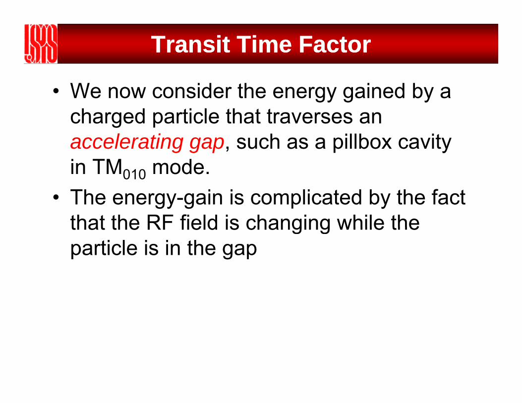
Transit Time FactorTransit Time Factor

• We now consider the energy gained by a charged particle that traverses an g paccelerating gap, such as a pillbox cavity in TM010 mode.010

• The energy-gain is complicated by the fact that the RF field is changing while thethat the RF field is changing while the particle is in the gap

Transit Time FactorTransit Time Factor• We will consider this problem by considering successively

more realistic (and complicated) models for the accelerating gap, where in each case the field varies sinusoidally in timegap, where in each case the field varies sinusoidally in time

• We also must consider the possibility that the energy gain depends on particle radius

+q

EE

Acceleration by TimeAcceleration by Time--Varying FieldsVarying Fields

L

Consider infinite parallel plates separated by a distance L with sinusoidal voltage applied, assume uniform E-field in gap (neglect holes)

)cos()( 0 φω +== tEtEE zz

+q

L

where at t=0, the particle is at the t f th ( 0) d th xcenter of the gap (z=0), and the

phase of the field relative to the crest is φ

B t t is a f nction of position t t( ) ith

Ez

x

y

∫=z

zvdzzt

0 )()( V0

+ -∼

But t is a function of position t=t(z), with y

∫ zv0 )(

∫∫2/2/ LL

The energy gain in the accelerating gap is

∫∫ −−+==Δ

2/

2/0

2/

2/))(cos(

L

L

L

L z dzztqEdzEqW φω

Energy Gain in an Accelerating GapEnergy Gain in an Accelerating Gap

• Assume the velocity change through the gap is small, so that t(z) = z/v,and

22βλπ

βλπωω z

czc

vzt 22

==≈

∫−

−=Δ2/

2/0 )sinsincos(cos

L

L

dzttqEW φωφω This is an odd-function of z

∫ ∫ ⎟⎟⎠

⎞⎜⎜⎝

⎛−⎟⎟

⎠

⎞⎜⎜⎝

⎛=Δ

2/

2/

2/

2/00

2sinsin2coscosL

L

L

L

dzzqEdzzqEWβλπφ

βλπφ

of z

− − ⎠⎝⎠⎝2/ 2/L L βλβλ

2/

02sincos

LzqEW ⎥⎤

⎢⎡

=Δπβλφ

2/0 2 L

q−⎥⎦

⎢⎣ βλπ

φ

Energy Gain and Transit Time FactorEnergy Gain and Transit Time Factor

φβλπβλπ cos

/)/sin(

0 LL

LqEW =Δ

φcos0TqVW =Δβλπ )/sin( L

βλπβλπ

/)/sin(

LLT =

• Compare to energy gain from static DC field: φcosTWW DCΔ=Δ

• T is the transit-time factor: a factor that takes into account the time-variation of the field during particle transit through the gap

φ i h h h d f h• φ is the synchronous phase, measured from the crest

TransitTransit--Time FactorTime Factor

1

1.2

0.6

0.8

Fact

or

0.2

0.4

ansi

t-Tim

e

-0.2

00 1 2 3 4 5

Tra

-0.4

L/βλ

For efficient acceleration by RF fields, we need to properly match the gap length L to the distance that the particle travels in one RF wavelength, βλ

Transit Time Factor for Real RF GapsTransit Time Factor for Real RF Gaps

• The energy gain just calculated for infinite planes is the same as that for an on-axis particle accelerated in a pillbox cavity neglecting the beam holes

• A more realistic accelerating field depends on r, z

• Calculate the energy gain as before:

)cos(),(),,( φω +== tzrEtzrEE zz

Calculate the energy gain as before:

∫∫ +==Δ2/2/

))(cos()0(LL

dzztzEqdzEqW φω∫∫ −−+==Δ

2/2/))(cos(),0(

LL z dzztzEqdzEqW φω

∫Δ2/

)ii)(0(L

dttEW φφ∫−

−=Δ2/

)sinsincos)(cos,0(L

dzttzEqW φωφω L

TransitTransit--time Factortime Factor

∫ =2/

0)(sin)0(L

dzztzE ω

• Choose the origin at the electrical center of the gap, defined as

ωcos)0(2/

⎥⎤

⎢⎡∫

L

tdzzE

∫−

=2/

0)(sin),0(L

dzztzE ω• This gives

φω

φ cos),0(

cos),0(),0(cos 2/

2/

2/2/

2/0

⎥⎥⎥⎥

⎦⎢⎢⎢⎢

⎣

⎥⎦

⎤⎢⎣

⎡==Δ

∫

∫∫ −

−L

L

LL

L dzzE

tdzzEdzzEqTqVW

2/ ⎦⎣ −L

• From which we identify the general form of the transit-time factor as

∫

∫−= 2/

2/

2/

cos),0(

L

L

L

tdzzET

ω

∫− 2/

),0(L

dzzE

TransitTransit--time Factortime Factor• Assuming that the velocity change is small in the gap,

then kzzzt ==≈

βλπωω 2

• The transit time factor can be expressed asv βλ

∫=≡2/

)cos()0(1)0()(L

dzkzzEkTkT ∫−

=≡2/0

)cos(),0(),0()(L

dzkzzEV

kTkT

∫−=2/

2/0 ),0(L

LdzzEV βλ

π2=kβ

Radial Dependence of TransitRadial Dependence of Transit--time Factortime Factor

W l l t d th T it ti f t f i ti l W• We calculated the Transit-time factor for an on-axis particle. We can extend this analysis to the transit-time factor and energy gain for off-axis particlesThi i i t t b th l t i fi ld i illb it d• This is important because the electric-field in a pillbox cavity decreases with radius (remember TM010 fields)

∫=2/

)cos(),(1),(L

dzkzzrEkrT

)()(),( 0 KrIkTkrT =• Where I is the modified Bessel function of order zero and

∫− 2/0

)(),(),(LV

γβλπ2

=K

• Where I0 is the modified Bessel function of order zero, and

Giving for the energy gain• Giving for the energy gain

φcos)()( 00 KrIkTqVW =Δ

which is the on-axis result modified by the r-dependent Bessel function

Realistic Geometry of an RF GapRealistic Geometry of an RF Gap

A l ti fi ld t d ift t b b di ( ) i t t• Assume accelerating field at drift-tube bore radius (r=a) is constant within the gap, and zero outside the gap within the drift tube walls

⎭⎬⎫

⎩⎨⎧

≤≤≤

==zg

gzEzarE g

2/02/0

),(

• Using the definition of transit-time factor:

∫−

=2/

2/0

)cos(),(1),(L

L

dzkzzrEV

krT

• we get)2/i (kE E

βλπλπ )/sin()/2( gaJ

2/)2/sin(

)()(

00 kg

kgKaIgE

kTV g=)/2(0

0 λπaJgE

V g=

• Finallyβλπβλπλπ

/)/sin(

)()/2()()()(),(

0

000 g

gKaIaJKrIKrIkTkrT ==

Finally,

What about the drift tubes?What about the drift tubes?Th ff f f li d i l id• The cutoff frequency for a cylindrical waveguide is Th d ift t b h t ff f b l hi h

Rcc /405.2=ω• The drift tube has a cutoff frequency, below which

EM waves do not propagateThe propagation factor k is• The propagation factor k is

0405.2405.222

2 <⎟⎟⎠

⎞⎜⎜⎝

⎛−⎟⎟

⎠

⎞⎜⎜⎝

⎛=z RR

k

• So the electric field decays exponentially with penetration distance in the drift tube:

⎟⎠

⎜⎝

⎟⎠

⎜⎝ holec RR

penetration distance in the drift tube:

E l 1 GH it ith 1 b h l

tizktzkiitkziz eeEeEeEE ωωω −−−− === 0

)(0

)(0

• Example: 1 GHz cavity with r=1cm beam holes:

Power and Acceleration Figures of MeritPower and Acceleration Figures of Merit

• Quality Factor – “goodness” of an oscillator

Shunt Impedance:

PUQ ω

=

V 2• Shunt Impedance:

– “Ohms law” resistance

• Effective Shunt Impedance:

PVrs

0=

22

0 )( TVEffective Shunt Impedance:– Impedance including TTF

• Shunt Impedance per unit

20 )( TrPTVr s==

ErZ s20==p p

length

• Effective Shunt Impedance/unit

LPL /

TErZT )( 202 ==p

length:

• “R over Q”

LPLZT

/==

TVr 2)(– Efficiency of acceleration per unit

of stored energyUTV

Qr

ω0 )(

=

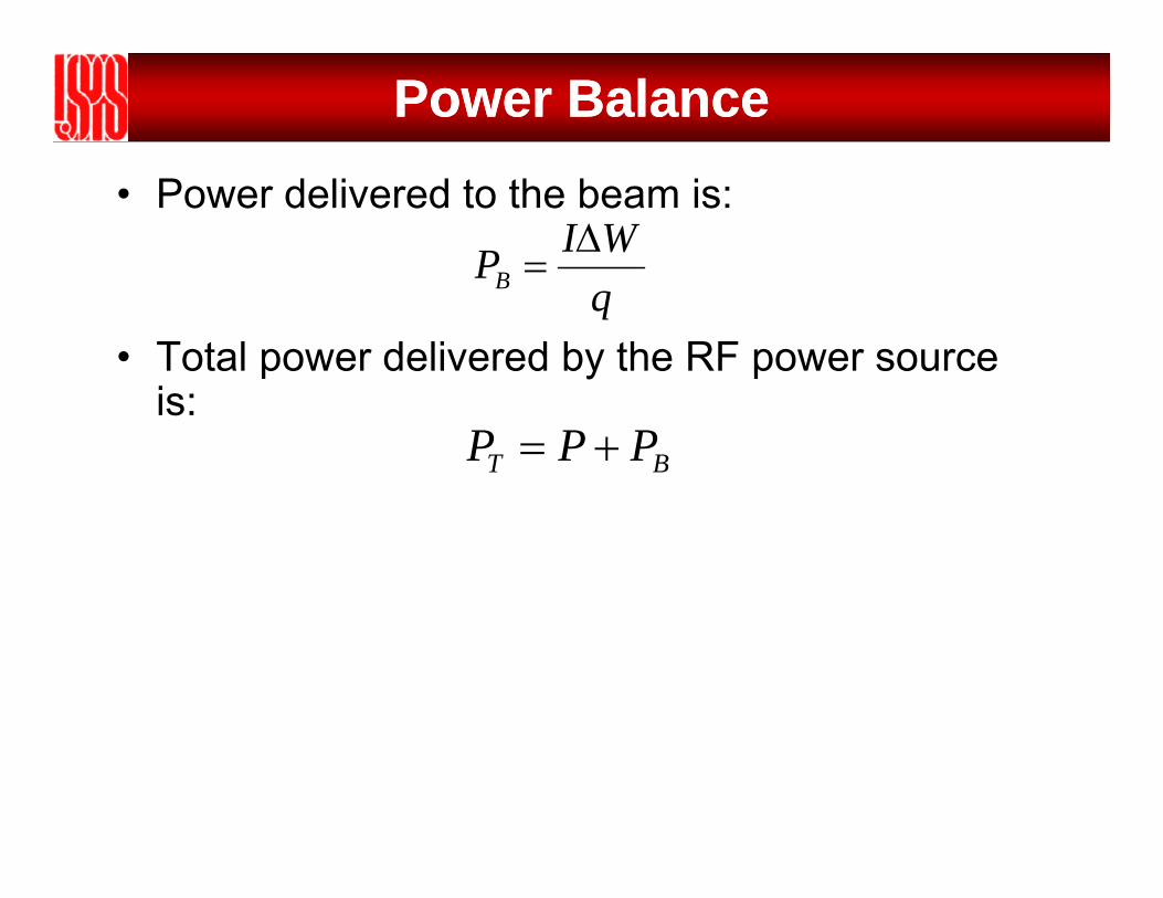
Power BalancePower Balance• Power delivered to the beam is:

WIPBΔ

=

• Total power delivered by the RF power source i

qB

is:BT PPP +=

Coupled RF Cavities and Coupled RF Cavities and Normal ModesNormal Modes

Now, let’s make a real linacNow, let’s make a real linac

• We can accelerate particles in a pillbox cavityy

• Real linacs are made by stringing together a series of pillbox cavitiesa series of pillbox cavities.

• These cavity arrays can be constructed from independently powered cavities orfrom independently powered cavities, or by “coupling” a number of cavities in a single RF structuresingle RF structure.

Coupling of two cavitiesCoupling of two cavities• Suppose we couple two RF cavities

together:• Each is an electrical oscillator with the

same resonant frequencysame resonant frequency• A beampipe couples the two cavities

• Remember the case of mechanical coupling of two oscillators:p g• Two mechanical modes are possible:

– The “zero-mode”: φA- φB=0, where each oscillates at natural frequency– The “pi-mode”: φA- φB=π, where each oscillates at a higher frequency

Coupling of electrical oscillatorsCoupling of electrical oscillators• Two coupled oscillators, each

with same resonant frequency:• Apply Kirchoff’s laws to each

i iLC12

0 =ω

i1 i2

circuit:

0)(1)( 211 =Ω+Ω

+Ω=∑ MjiCj

iLjiV

C C• Gives 0)1(

2

22

20

1 =+Ω

−

MLMii

ω

ω

0)1( 120

2 =+Ω

−LMii ω

• Which can be expressed as:

⎞⎛⎞⎛⎞⎛ 22 1//1 iik⎟⎟⎠

⎞⎜⎜⎝

⎛Ω

=⎟⎟⎠

⎞⎜⎜⎝

⎛⎟⎟⎠

⎞⎜⎜⎝

⎛

2

12

2

120

20

20

20 1

/1///1

ii

ii

kkωωωω

• You may recognize this as an

LMk /=

• You may recognize this as an eigenvalue problem q

qq XXM

vv2

1~Ω

=

Coupling of electrical oscillatorsCoupling of electrical oscillators• There are two normal-mode eigenvectors and associated

eigenfrequecies• Zero-mode:

⎟⎟⎠

⎞⎜⎜⎝

⎛=

11

0Xk+

=Ω1

00

ω

⎟⎟⎠

⎞⎜⎜⎝

⎛−

=1

1πX k−

=Ω1

0ωπ

• Pi-mode:

⎠⎝ 1

• Like the coupled pendula, we have 2 normal modes, one for in-phase oscillation (“Zero-mode”) and another for out of phase p ( ) poscillation (“Pi-mode”).

• It is important to remember that both oscillators have resonant frequencies Ω, different from the natural (uncoupled) frequency.q , ( p ) q y

Normal modes for many coupled cavitiesNormal modes for many coupled cavities

N 1 l d ill t h N 1 l d f ill ti• N+1 coupled oscillators have N+1 normal-modes of oscillation• Normal mode spectrum:

0ω=Ω

• Where q=0,1,…N is the d b

)/cos(1 Nqkq π+=Ω

mode number• Not all are useful for

particle acceleration• Standing wave

structures of coupled cavities are all driven so th t th bthat the beam sees either the zero or πmode

Example for a 3Example for a 3--cell Cavity: Zerocell Cavity: Zero--mode mode ExcitationExcitation

ωt=0

ωt=π/4ωt=π/4

ωt=π/2

t 3 /4ωt=3π/4

ωt=π

ωt=5π/4

ωt=3π/2

ωt=7π/4

ωt=2π

Example for a 3Example for a 3--cell Cavity: Picell Cavity: Pi--mode Excitationmode Excitation

ωt=0

ωt=π/4ωt=π/4

ωt=π/2

t 3 /4ωt=3π/4

ωt=π

ωt=5π/4

ωt=3π/2

ωt=7π/4

ωt=2π

Synchronicity condition in multicell RF Synchronicity condition in multicell RF structuresstructures

TM010 CavitiesDrift spaces

l1 l2 l3 l4 l5

β1 β2 β3 β4β5

• Suppose we want a particle to arrive at the center of each gap at φ=0. Then we would have to space the cavities so that the RF phase advanced by

l1 l2 l3 l4 l5

advanced by – 2π if the coupled cavity array was driven in zero-mode– Or by π if the coupled cavity array was driven in pi-mode

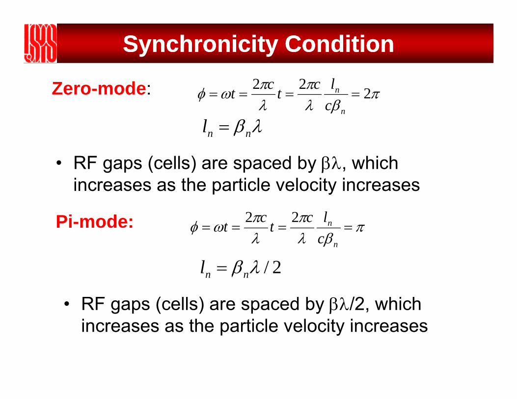
Synchronicity ConditionSynchronicity Condition

Zero-mode: πβλ

πλπωφ 222

====n

n

clctct

λβl λβnnl =

• RF gaps (cells) are spaced by βλ, which increases as the particle velocity increases

Pi-mode: πππωφ nlctct 22Pi mode: πβλλ

ωφ ====n

n

ctt

2/λβnnl = βnn

• RF gaps (cells) are spaced by βλ/2, which increases as the particle velocity increasesincreases as the particle velocity increases

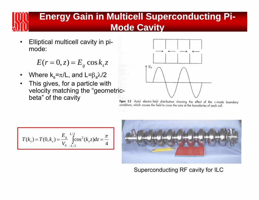
Energy Gain in Multicell Superconducting PiEnergy Gain in Multicell Superconducting Pi--Mode CavityMode Cavity

• Elliptical multicell cavity in pi-mode:

zkEzrE cos)0( ==

• Where ks=π/L, and L=βsλ/2 • This gives, for a particle with

zkEzrE sg cos),0( ==

velocity matching the “geometric-beta” of the cavity

)()0()(2/

2 π∫ dk

EkTkT

Lg

4)(cos),0()(

2/

2

0

=== ∫−

dzzkV

kTkTL

sg

ss

Superconducting RF cavity for ILC

Examples of RF Cavity Examples of RF Cavity StructuresStructures

Alvarez Drift Tube LinacAlvarez Drift Tube Linac• DTL consists of a long “tank”

excited in TM010 mode (radius determines frequency)frequency)

• Drift tubes are placed along the beam-axis so that the accelerating gaps satisfy synchronicity condition withsynchronicity condition, with nominal spacing of βλ

• The cutoff frequency for EM propagation within the drift tubes is much greater than the resonant frequency of the tank (ωc=2.405c/R)

• Each tube (cell) can be ac tube (ce ) ca beconsidered a separate cavity, so that the entire DTL structure is a set of coupled cavity resonators excited in ythe zero-mode

ZeroZero--mode excitation of a Drift Tube Linac mode excitation of a Drift Tube Linac TankTank

• φ=ωt=0, Ez=E0

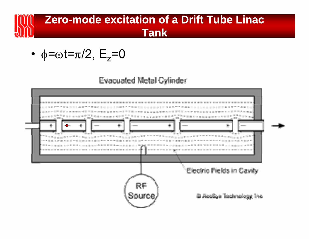
ZeroZero--mode excitation of a Drift Tube Linac mode excitation of a Drift Tube Linac TankTank

• φ=ωt=π/2, Ez=0

ZeroZero--mode excitation of a Drift Tube Linac mode excitation of a Drift Tube Linac TankTank

• φ=ωt=π, Ez=-E0

ZeroZero--mode excitation of a Drift Tube Linac mode excitation of a Drift Tube Linac TankTank

• φ=ωt=3π/2, Ez=0

ZeroZero--mode excitation of a Drift Tube Linac mode excitation of a Drift Tube Linac TankTank

• φ=ωt=2π, Ez=E0

Alvarez Drift Tube LinacAlvarez Drift Tube Linac• DTLs are used to accelerate protons from ∼1• DTLs are used to accelerate protons from ∼1

MeV to ∼100 MeV• At higher energies, the drift tubes become

long and unwieldy• DTL frequencies are in the 200 400 MHz• DTL frequencies are in the 200-400 MHz

range

Coupled Cavity LinacCoupled Cavity Linac• Long array of coupled cavities driven in π/2 mode• Every other cavity is unpowered in the π/2 mode• These are placed off the beam axis in order to minimize the length of the

linaclinac• To the beam, the structure looks like a π mode structure• Actual CCL structures contain hundreds of coupled cavities, and therefore

have hundreds of normal-modes. Only the π/2 mode is useful for beam acceleration.acceleration.

• The cell spacing varies with beam velocity, with nominal cell length βλ/2

Coupled Cavity Linac ExamplesCoupled Cavity Linac Examples

Other Types of RF StructuresOther Types of RF Structures

Other Types of RF StructuresOther Types of RF Structures

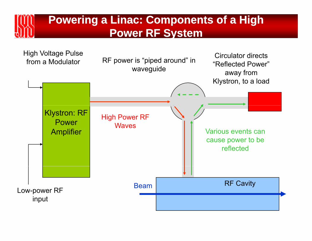
Powering a Linac: Components of a High Powering a Linac: Components of a High Power RF SystemPower RF System

RF power is “piped around” in waveguide

High Voltage Pulse from a Modulator

Circulator directs “Reflected Power”

away fromaway from Klystron, to a load

Klystron: RF Power

Amplifier

High Power RF Waves

Various events can pcause power to be

reflected

Low-power RF i t

RF CavityBeam

input

Klystron OperationKlystron Operation

• A Klystron is an amplifier for radio-frequency waveswaves

• A Klystron is a little accelerator/RF cavity system all its own

• Electrons are produced from a gunA hi h l l l l• A high-voltage pulse accelerates an electron beam

• Low power RF excites the first cavity, which bunches the electrons

• These electrons “ring the bell” in the next cavity• A train of electron bunches excites the cavity,

generating RF power

Linac RF SystemsLinac RF Systems

W idKlystron Gallery

Waveguide, circulators and loads

dC

avity

Fie

ld

Cavity Field vs. time without beam

Time

C

EExamplexample Beam Pulse StructureBeam Pulse Structure

16.7ms (1/60 Hz)

15 7

Macro-pulseStructure ( d b th

1ms15.7ms(made by the

High power RF)

645 ns 300 ns

945 ns (1/1.059 MHz)Mini-pulseStructure (made by the choppers)

2.4845 ns (1/402.5 MHz)

260 micro-pulses

choppers)

Micro-pulsestructure(made by the RFQ)

43

Example ProblemExample ProblemC id 10 l (1/ 1 7 10 8 Ω ) TM• Consider a 10-cm-long copper (1/σ =1.7x10-8 Ω m) TM010pillbox cavity with resonant frequency of 500 MHz and axial field E=1.5MV/m.a) For a proton with kinetic energy of 100 MeV, calculate the transit-

time factor ignoring the effects of the aperture, and assuming that the velocity remains constant in the gapy g p

b) If the proton arrives at the center of the gap 45 degrees before the crest, what is the energy gain?

c) Calculate the RF power dissipated in the cavity wallsc) Calculate the RF power dissipated in the cavity wallsd) Suppose this cavity is used to accelerate a 100 mA beam. What is

the total RF power that must be provided by the klystron?e) Calculate the shunt impedance the effective shunt impedance thee) Calculate the shunt impedance, the effective shunt impedance, the

shunt impedance per unit length, and the effective shunt impedance per unit length

f) Assume the drift tube bore radius is 2 cm Calculate the transit-f) Assume the drift tube bore radius is 2 cm. Calculate the transit-time factor, including the aperture effects, for the proton on-axis, and off-axis by 1 cm. Assume that

4/1)( 20 xxI += 4/1)( 2

0 xxJ −=