Rewiring WorldTrade. Part I: A Binary Network … WorldTrade. Part I: A Binary Network Analysis ......
18
Transcript of Rewiring WorldTrade. Part I: A Binary Network … WorldTrade. Part I: A Binary Network Analysis ......


Rewiring World Trade. Part I: A Binary Network Analysis
Tiziano SquartiniCSC and Department of Physics, University of Siena, Via Roma 56, 53100 Siena (Italy)
Giorgio FagioloLEM, Sant’Anna School of Advanced Studies, 56127 Pisa (Italy)
Diego GarlaschelliLEM, Sant’Anna School of Advanced Studies, 56127 Pisa (Italy) andInstituut-Lorentz for Theoretical Physics, Leiden Institute of Physics,
University of Leiden, Niels Bohrweg 2, 2333 CA Leiden (The Netherlands)(Dated: March 7, 2011)
The international trade network (ITN) has received renewed multidisciplinary interest due to re-cent advances in network theory. However, it is still unclear whether a network approach conveysadditional, nontrivial information with respect to traditional international-economics analyses thatdescribe world trade only in terms of local (first-order) properties. In this and in a companionpaper, we employ a recently-proposed randomization method to assess in detail the role that localproperties have in shaping higher-order patterns of the ITN in all its possible representations (bi-nary/weighted, directed/undirected, aggregated/disaggregated) and across several years. Here weshow that, remarkably, all the properties of all binary projections of the network can be completelytraced back to the degree sequence, which is therefore maximally informative. Our results implythat explaining the observed degree sequence of the ITN, which has not received particular attentionin economic theory, should instead become one the main focuses of models of trade.
PACS numbers: 89.65.Gh; 89.70.Cf; 89.75.-k; 02.70.Rr
I. INTRODUCTION
The network of import/export trade relationshipsamong all world countries, known in the literature as theInternational Trade Network (ITN) or the World TradeWeb (WTW), has received a renewed multidisciplinaryinterest in recent years [1–13], due to impressive advancesin both empirical and theoretical approaches to the studyof complex networks [14–16]. A number of robust pat-terns in the structure of this network have been empir-ically observed, both in its binary (when only the pres-ence of a trade interaction is considered, irrespective ofits intensity) and weighted (when also the magnitude oftrade flows is taken into account) description. These styl-ized facts include local properties as well as higher-orderpatterns. Local properties involve direct (first-order) in-teractions alone, resulting in simple quantities such asnode degree (the number of trade partners of a country),node strength (total trade volume of a country), and theirdirected-network analogues (i.e., when these statistics arecomputed taking into account edge/trade directionality).Higher-order characteristics are more complicated struc-tural properties that also involve indirect interactions, i.e.topological paths connecting a country to the neighborsof its neighbors, or to countries farther apart. Exam-ples include degree-degree correlations, average nearest-neighbor indicators, and clustering coefficients, to namejust a few of them.
In general, local and higher-order topological proper-ties are not independent of each other. In particular,even if one assumes that the network is formed as the
result of local constraints alone, with higher-order prop-erties being only the mere outcome of specifying theseconstraints, it turns out that so-called structural corre-lations are automatically generated. Structural corre-lations sometimes appear as complicated patterns thatmight be confused with genuine correlations involvinghigher-order statistics, and interpreted as the presenceof an additional level of topological organization. There-fore, in any real network it is important to characterizestructural correlations and filter them out in order to as-sess whether nontrivial effects due to indirect interactionsare indeed present.
In the specific case of the ITN, this problem is partic-ularly important to assess whether the network formal-ism is really conveying additional, nontrivial informationwith respect to traditional international-economics anal-yses, which instead explain the empirical properties oftrade in terms of country-specific macroeconomic vari-ables alone. Indeed, as we discuss in more detail below,the standard economic approach to the empirics of inter-national trade [17] has traditionally focused its analyseson the statistical properties of country-specific indica-tors like total trade, trade openness (ratio of total tradeto GDP, i.e. Gross Domestic Product), number of tradepartners, etc., that can be easily mapped to what, in thejargon of network analysis, one denotes as local proper-ties or first-order node characteristics.
In this and in a companion paper [18], we explicitlyaddress this problem and exploit a recently proposed an-alytical method [19] to obtain, for any given topologi-cal property of interest, the value of the corresponding
2
quantity averaged over the family of all randomized vari-ants of the ITN that preserve the observed local proper-ties. This allows us to identify empirical deviations fromlocally-induced structural correlations. In this first pa-per, we focus on the ITN as a binary network. We findthat higher-order patterns of all binary (either directedor undirected) projections of the ITN are completely ex-plained by local properties alone (the degree sequences).This result is robust to different levels of commodity ag-gregation: even if with an increasing scatter, the degreesequence preserves its complete informativeness as moredisaggregated and sparser commodity-specific networksare considered.
¿From an international-trade perspective, our resultsindicate that binary network descriptions of trade canbe significantly simplified by considering the degree se-quence(s) only. In other words, in any binary represen-tation of the ITN, the degree sequence turns out to bemaximally informative, since its knowledge conveys al-most the entire information about the topology of thenetwork. In the companion paper [18], we show that thepicture changes completely when considering the ITN asa weighted network. We find that the ITN is an excel-lent example of a network whose local topological prop-erties cannot be deduced from its local weighted proper-ties. These results highlight an important limitation ofcurrent economic models of trade, that do not aim at ex-plaining or reproducing the observed degree sequence butfocus more on the structure of weights [20]. The observedextreme informativeness of the degree sequence leads usto conclude that such models should be substantially re-vised in order to explicitly include the degree sequenceof the ITN among the key properties to reproduce.
II. DATA AND METHODS
This Section describes the data we use to construct thevarious representations of the network in this and in thefollowing paper [18], and briefly summarizes the methodwe employ to obtain expected properties over randomizedcounterparts of a network.
A. The International Trade Network
We use yearly bilateral data on exports and importsfrom the United Nations Commodity Trade Database(UN COMTRADE) [? ] from year 1992 to 2002. Wehave chosen this database because, despite its relativelyshort time interval (11 years), it contains trade data be-tween countries disaggregated across commodity cate-gories. This allows us to perform our analyses both at theaggregate level (total trade flows) and at the commodity-specific level, e.g. investigating whether local propertiesare sufficient to explain higher-order ones in commodity-specific networks of trade.
In order to perform a temporal analysis and allow com-parisons across different years, we restrict ourselves to abalanced panel of N = 162 countries that are present inthe data throughout the time interval considered. As tothe level of disaggregation, we choose the classificationof trade values into C = 97 possible commodities listedaccording to the Harmonized System 1996 (HS1996) [?]. Accordingly, for a given year t we consider the tradevalue ecij(t) corresponding to exports of the particularcommodity c (c = 1, . . . C). Since, for every commodity,exports from country i to country j are reported twice(by both the importer and the exporter) and the two fig-ures do not always match, we follow Ref. [13] and onlyemploy the flow as reported by the importer. Besidescommodity-specific data, we also compute the total valuee0ij(t) of exports from country i to country j as the sumover the exports of all C = 97 commodity classes:
e0ij(t) ≡
C∑
c=1
ecij(t) (1)
The particular aggregation procedure described above,which coincides with the one performed in Ref. [13], al-lows us to compare our analysis of the C commodity-specific networks with a (C + 1)-th aggregate network,avoiding possible inconsistencies between aggregated anddisaggregated trade data. We stress that the resulting ag-gregated network data are in general different from thoseused in other analyses [3, 4, 12] of the same network.Nonetheless, as we show below, when we analyze net-work properties that have also been studied in previousstudies of aggregate trade, we find perfect agreement.The quantities {ecij(t)} (where c = 0, . . . C) defined
above are the fundamental data that allow us to obtaindifferent possible representations of the trade network, aswell as the corresponding randomized counterparts (seebelow for the units of measure we adopted). When weregard the ITN as a weighted directed network, we definethe weight of the link from country i to country j in yeart for commodity c as
wcij(t) ≡ ⌊ecij(t)⌉ c = 0, . . . C (2)
where ⌊x⌉ ∈ N denotes the nearest integer to the non-negative real number x. When we adopt a weightedbut undirected (symmetrized) description, we define theweight of the link between countries i and j in year t forcommodity c as
wcij(t) ≡ wc
ji(t) ≡
⌊
ecij(t) + ecji(t)
2
⌉
c = 0, . . . C (3)
Therefore, in both the directed and undirected case,wc
ij(t) is an integer quantity. Since in both cases we shallbe interested in tracking the temporal evolution of mostquantities, we also define rescaled weights (relative to thetotal yearly trade flow) as follows:
wcij(t) ≡
wcij(t)
wctot(t)
c = 0, . . . C (4)

3
HS Code Commodity Value (USD) Value per link (USD) % of aggregate trade84 Nuclear reactors, boilers, machinery and
mechanical appliances; parts thereof5.67× 1011 6.17× 10⁷ 11.37%
85 Electric machinery, equipment and parts;sound equipment; television equipment
5.58× 10¹¹ 6.37× 10⁷ 11.18%
27 Mineral fuels, mineral oils & products oftheir distillation; bitumin substances; min-eral wax
4.45× 10¹¹ 9.91× 10⁷ 8.92%
87 Vehicles, (not railway, tramway, rollingstock); parts and accessories
3.09× 10¹¹ 4.76× 10⁷ 6.19%
90 Optical, photographic, cinematographic,measuring, checking, precision, medical orsurgical instruments/apparatus; parts &accessories
1.78× 10¹¹ 2.48× 10⁷ 3.58%
39 Plastics and articles thereof. 1.71× 10¹¹ 2.33× 10⁷ 3.44%29 Organic chemicals 1.67× 10¹¹ 3.29× 10⁷ 3.35%30 Pharmaceutical products 1.4× 10¹¹ 2.59× 10⁷ 2.81%72 Iron and steel 1.35× 10¹¹ 2.77× 10⁷ 2.70%71 Pearls, precious stones, metals, coins, etc 1.01× 10¹¹ 2.41× 10⁷ 2.02%10 Cereals 3.63× 10¹⁰ 1.28× 10⁷ 0.73%52 Cotton, including yarn and woven fabric
thereof3.29× 1010 6.96× 10⁶ 0.66%
9 Coffee, tea, mate & spices 1.28× 10¹⁰ 2.56× 10⁶ 0.26%93 Arms and ammunition, parts and acces-
sories thereof4.31× 109 2.46× 10⁶ 0.09%
ALL Aggregate (all 97 commodities) 4.99× 10¹² 3.54× 10⁸ 100.00%
TABLE I: The 14 most relevant commodity classes (plus aggregate trade) in year 2003 and the corresponding total trade value(USD), trade value per link (USD), and share of world aggregate trade. From Ref. [13].
where in the directed case wcij(t) is given by Eq. (2)
and wctot(t) ≡
∑
i
∑
j 6=i wcij(t) (the double sum runs
over all N(N − 1) ordered pairs of vertices), whilein the undirected case wc
ij(t) is given by Eq. (3) andwc
tot(t) ≡∑
i
∑
j<i wcij(t) (the double sum runs over
all the N(N − 1)/2 unordered pairs). In such a way,trend effects are washed away and we obtain adimen-sional weights that are automatically deflated, allowingconsistent comparisons across different years and differ-ent commodities.In the binary representations of the network, we draw a
link from i to j whenever the corresponding weight wcij is
strictly positive. If Θ(x) denotes the step function (equalto 1 if x > 0 and 0 otherwise), the adjacency matrix of thebinary projection of the network in year t for commodityc is
acij(t) ≡ Θ[wcij(t)] c = 0, . . . C (5)
where wcij(t) is given either by Eq. (2) or by Eq. (3),
depending on whether one is interested in a directed orundirected binary projection of the network respectively.For each of the C + 1 commodity categories, we
can consider four network representations (binary undi-rected, binary directed, weighted undirected, weighteddirected). When reporting our results, we will firstdescribe the aggregated networks (c = 0) and thenthe disaggregated (commodity-specific) ones. In par-ticular, among the 97 commodity classes, we will fo-
cus on the 14 particularly relevant commodities identi-fied in Ref. [13], which are reported in table I. These14 commodities include the 10 most traded commodi-ties (c = 84, 85, 27, 87, 90, 39, 29, 30, 72, 71 according tothe HS1996) in terms of total trade value (following theranking in year 2003 [13]), plus 4 classes (c = 10, 52, 9, 93according to the HS1996) which are less traded but morerelevant in economic terms. Taken together, the 10 mosttraded commodities account for 56% of total world tradein 2003; moreover, they also feature the largest valuesof trade value per link (also shown in the table). The14 commodities considered account together for 57% ofworld trade in 2003. As an intermediate level of aggrega-tion, we shall also consider the networks formed by thesum of these 14 commodities. The original data {ecij(t)}are available in current U.S. dollars (USD) for all com-modities; however, due to the different trade volumesinvolved, we use different units of measure for differentlevels of aggregation [? ].
B. Controlling for local properties
As we mentioned, our main interest in the present workis assessing whether higher-order properties of the ITNcan be simply traced back to local properties, which arethe main focus of traditional macroeconomic analyses ofinternational trade. Such standard country-specific prop-erties include: total exports, total imports, total trade

4
(sum of total exports and total imports), trade openness(ratio of total trade to GDP), the number of countrieswhom a country exports to and imports from, the totalnumber of trade partners (irrespective of whether theyare importers or exporters, or both). All these quan-tities can be simply obtained as local sums over directinteractions (countries one step apart) in a suitable rep-resentation of the network.For instance, the number of trade partners of country i
is simply the number of neighbors of node i in the binaryundirected projection, i.e. the degree
ki ≡∑
j 6=i
aij (6)
In the above equation and in what follows, we drop thedependence of topological quantities on the particularyear t for simplicity. We also drop the superscript c speci-fying a particular commodity, as all the formulas hold forany c. This means that, if the aggregated network of totaltrade is considered, then aij and wij represent the aggre-gate quantities a0ij and w0
ij , where the commodity c = 0formally represents the sum over all commodities, as inEq. (1). Otherwise, if the commodity-specific networkinvolving only the trade of the particular commodity c(with c > 0) is considered, then aij and wij represent thevalues acij and wc
ij for that commodity.The number of countries whom a country exports to
and imports from are simply the two directed analogues(the out-degree kouti and the in-degree kini respectively)of the above quantity in the binary directed description:
kouti ≡∑
j 6=i
aij (7)
kini ≡∑
j 6=i
aji (8)
Similarly, as evident from Eq. (3), country i’s totaltrade coincides with twice the sum of weights reachingnode i in the weighted undirected representation, i.e. thestrength
si ≡∑
j 6=i
wij (9)
Finally, total exports (imports) of country i are simplythe sum of out-going (in-coming) weights in the weighteddirected representation of the ITN. These quantities areknown as the out-strength souti and in-strength sini of nodei:
souti ≡∑
j 6=i
wij (10)
sini ≡∑
j 6=i
wji (11)
Another country-specific property which is widely usedas an explanatory variable of trade patterns is the GDP
or the per capita GDP (i.e. the ratio of GDP to popula-tion). This property is sometimes used to rescale tradevalues, as in the case of trade openness which is definedas a country’s ratio of total trade to GDP. Unlike thequantities discussed above, the GDP is not a topologicalentity. Nonetheless, it is empirically observed to be pos-itively (and strongly) correlated with the degree [3] andwith node strength [12] (we will comment more on this inSection III). Therefore, even if this is not the main aimof the present work, one should be aware that assessingthe role of local topological properties also indirectly im-plies, to a large extent, assessing the role of the GDP ofcountries.
Whether the topological architecture of the various de-scriptions of the ITN can be understood simply in termsof the above local properties, or whether there are ad-ditional organizing principles generating a more compli-cated structure, is an important open question. Ulti-mately, this amounts to assess the effects of indirect in-teractions in the world trade system. Indeed, a wealthof results about the analysis of international trade havealready been derived in the macroeconomics literature[17] without making explicit use of the network descrip-tion, and focusing on the above country-specific quan-tities alone. Whether more recent analyses of trade,directly inspired by the network paradigm [1–12], areindeed conveying additional and nontrivial informationabout the structure of international import/export flows,crucially depends on the answer to the above question.Some network-inspired studies have already tried to ad-dress this problem, but with ambiguous results. In somecases, it was suggested that local properties are enoughto explain higher-order patterns [3, 6, 21], while in othersthe opposite conclusion was reached [22]. However, pre-vious analyses of the ITN focused on heterogeneous rep-resentations (either binary [2, 3] or weighted [6, 10, 22],either directed [4, 5, 23] or undirected [2, 3], either aggre-gated [2, 3, 10] or disaggregated [13]) and using differentdatasets, making consistent conclusions impossible.
In this work, we address this problem in more detailand we separately consider all the four possible levelsof description of the network (binary/weighted and di-rected/undirected), for both commodity-specific and ag-gregate trade data. For each of these versions of thesame network, we compare the empirical structural prop-erties with their randomized counterparts, obtained ineach case by specifying the corresponding local proper-ties alone, and generating a collection of otherwise max-imally random graphs as a null model. Moreover, weperform a temporal analysis and check the robustness ofthese results over time. Therefore we obtain, for the firsttime in this type of study, a detailed and homogeneousassessment of the role of local properties across differentrepresentations of the trade network, using various levelsof commodity aggregation, and over several years. Forclarity, we divide our analysis in two parts. Here we con-sider only the possible binary projections of the ITN. Inthe companion paper [18], we study its possible weighted

5
representations.
C. The randomization method
Given a real network with N vertices, there are variousways to generate a family of randomized variants of it.The most popular one is the local rewiring algorithm pro-posed by Maslov and Sneppen [24, 25]. In this method,one starts with the real network and generates a series ofrandomized graphs by iterating a fundamental rewiringstep that preserves the desired properties. In the binaryundirected case, where one wants to preserve the degreeof every vertex, the steps are as follows: choose two edges,say (i, j) and (k, l); rewire these connections by swappingthe end-point vertices and producing two new candidateedges, say (i, l) and (k, j); if these two new edges are notalready present, accept them and delete the initial ones.After many iterations, this procedure generates a ran-domized variant of the original network, and by repeatingthis exercise a sufficiently large number of times, manyrandomized variants are obtained. By construction, allthese variants have exactly the same degree sequence asthe real-world network, but are otherwise random. Inthe directed and/or weighted case, proper extensions ofthe rewiring step defined above allow to generate analo-gous ensembles of randomized networks with fixed localconstraints. This method allows one to check whetherthe enforced properties are partially responsible for thetopological organization of the network. For instance,one can measure the degree correlations, or the cluster-ing coefficient, across the randomized graphs and com-pare them with the empirical values measured on thereal network. This method has been applied to variousnetworks, including the Internet and protein networks[24, 25]. Different webs have been found to be affectedin very different ways by local constraints, making theproblem interesting and not solvable a priori.The main drawback of the local rewiring algorithm is
its computational requirements. Since the method is en-tirely numerical, and analytical expressions for its resultsare not available, one needs to explicitly generate severalrandomized graphs, measure the properties of intereston each of them (and store their values), and finally per-form an average. This average is an approximation forthe actual expectation value over the entire set of al-lowed graphs. In order to have a good approximation,one needs to generate a large number M of network vari-ants. Thus, the time required to analyze the impact oflocal constraints on any structural property is M timesthe time required to measure that property on the orig-inal network, plus the time required to perform manyrewiring steps producing each of the M randomized net-works. The number of rewiring steps required to obtaina single randomized network is O(L) where L is the num-ber of links [19, 24, 25], and O(L) = O(N) for sparse net-works while O(L) = O(N2) for dense networks (the ITNis a dense network). Thus, if the time required to mea-
sure a given topological property on the original networkis O(Nk), the time required to measure the randomizedvalue of the same property is O(M · L) + O(M · Nk),which is O(M ·Nk) as soon as k ≥ 2.A recently proposed alternative method, which is in-
credibly faster due to its analytical character, is based onthe maximum-likelihood estimation of maximum-entropymodels of graphs [19]. In this method, one first specifiesthe desired set of local constraints {Ca}. Second, onewrites down the analytical expression for the probabilityP (G) that, subject to the constraints {Ca}, maximizesthe entropy
S ≡ −∑
G
P (G) lnP (G) (12)
where G denotes a particular graph in the ensemble,and P (G) is the probability of occurrence of that graph.This probability defines the ensemble featuring the de-sired properties, and being maximally random otherwise.Depending on the particular description adopted, thegraphs G can be either binary or weighted, and eitherdirected or undirected. Accordingly, the sum in Eq. (12),and in similar expressions shown later on, runs over allgraphs of the type specified. The formal solution to theentropy maximization problem can be written in terms ofthe so-called Hamiltonian H(G), representing the energy(or cost) associated to a given graph G. The Hamilto-nian is defined as a linear combination of the specifiedconstraints {Ca}:
H(G) ≡∑
a
θaCa(G) (13)
where {θa} are free parameters, acting as Lagrange multi-pliers controlling the expected values {〈Ca〉} of the con-straints across the ensemble. The notation Ca(G) de-notes the particular value of the quantity Ca when thelatter is measured on the graphG. In terms ofH(G), themaximum-entropy graph probability P (G) can be shownto be
P (G) =e−H(G)
Z(14)
where the normalizing quantity Z is the partition func-
tion, defined as
Z ≡∑
G
e−H(G) (15)
Third, one maximizes the likelihood P (G∗) to obtain theparticular graphG
∗, which is the real-world network thatone wants to randomize. This steps fixes the values ofthe Lagrange multipliers that finally allow to obtain thenumerical values of the expected topological propertiesaveraged over the randomized ensemble of graphs. Theparticular values of the parameters {θa} that enforce thelocal constraints, as observed on the particular real net-work G
∗, are found by maximizing the log-likelihood
λ ≡ lnP (G∗) = −H(G∗)− lnZ (16)

6
to obtain the real network G∗. It can be shown [21] that
this is equivalent to the requirement that the ensembleaverage 〈Ca〉 of each constraint Ca equals the empiricalvalue measured on the real network:
〈Ca〉 = Ca(G∗) ∀a (17)
Note that, unless explicitly specified, in what follows wesimplify the notation and simply write Ca instead ofCa(G
∗) for the empirically observed values of the con-straints. This is consistent with the notation alreadyadopted in Sections IIA and IIB. Once the parametervalues are found, they are inserted into the formal ex-pressions yielding the expected value
〈X〉 ≡∑
G
X(G)P (G) (18)
of any (higher-order) property of interest X. The quan-tity 〈X〉 represents the average value of the property Xacross the ensemble of random graphs with the same av-erage (across the ensemble itself) constraints as the realnetwork. For simplicity, we shall sometimes denote 〈X〉as a randomized property, and its value as the random-
ized value of X. In the Appendix we provide a detailedaccount of the expressions for the randomized propertiesappearing in the following analysis.
Technically, while the local rewiring algorithm gen-erates a microcanonical ensemble of graphs, contain-ing only those graphs for which the value of each con-straint Ca is exactly equal to the observed value Ca(G
∗),the maximum-likelihood method generates an expandedgrandcanonical ensemble where all possible graphs withN vertices are present, but where the ensemble average ofeach constraint Ca is equal to the observed value Ca(G
∗).One can show that the two methods converge for largenetworks [19]. However, the maximum-likelihood one isremarkably faster. Importantly, enforcing only local con-straints implies that P (G) factorizes as a simple productover pairs of vertices. This has the nice consequence thatthe expression for 〈X〉 is generally only as complicatedas that for X. In other words, after the preliminarymaximum-likelihood estimation of the parameters {θa}(which only takes seconds), in this method the time re-quired to obtain the exact expectation value of an O(Nk)property across the entire randomized graph ensemble isthe same as that required to measure the same propertyon the original real network, i.e. still O(Nk). Therefore,as compared to the local rewiring algorithm, which re-quires a timeO(M ·Nk), the maximum-likelihood methodis O(M) times faster, for arbitrarily large M . Using thismethod allows us to perform a detailed analysis, coveringall possible representations across several years, whichwould otherwise require an impressive amount of time.
III. THE ITN AS A BINARY UNDIRECTEDNETWORK
As we mentioned in Section IIA, in its binary rep-resentation the ITN is defined as a graph whose edgesreport the presence of trade relationships among worldcountries, irrespective of the intensity of these relation-ships. The binary representation of the ITN can be eitherundirected or directed, depending on whether one is in-terested in specifying the orientation of trade flows. Inboth cases, the complete information about the topologyof the network is encoded in the adjacency matrix A,whose entries {aij} are defined as in Eq. (5).In the simplest case, the presence of at least one of the
two possible trade relationships between any two coun-tries i and j (either from i to j or from j to i) is rep-resented as one undirected edge between nodes i and j.Therefore aij = aji and A is a symmetric matrix. In thisbinary undirected description, as shown in Eq. (6), thelocal constraints {Ca} are the degrees of all vertices, i.e.the degree sequence {ki}. Therefore, the randomizationmethod described in Section IIC works by specifying theconstraints {Ca} ≡ {ki} and allows us to write down theprobability of any graph G in the grandcanonical ensem-ble, which is uniquely specified by its generic adjacencymatrix A. As summarized in Appendix A, this allowsus to easily obtain the expectation value 〈X〉, formallydefined in Eq. (18), of any property X across the ensem-ble of binary undirected graphs whose expected degreesequence is equal to the empirical one. Note that, amongthe possible properties, the degree of vertices plays a spe-cial role, as its expectation value 〈ki〉 is exactly equal tothe empirical value ki, as required by the method. There-fore the values {ki} are useful control parameters and canbe efficiently used as independent variables in terms ofwhich other properties X can be visualized.For the sake of simplicity, in Sections IIIA and III B we
first report the results of this analysis on a single snap-shot of the commodity-aggregated network (the last yearin our temporal window, i.e. 2002). Then, we discussthe robustness of our results through time by trackingthem backwards in Section III C. We finally consider thedisaggregated analysis of commodity-specific networks inSection IIID.
A. Average nearest neighbor degree
We start with the analysis of the aggregated version ofthe ITN, representing the trade of all commodities (c = 0in our notation). In the following formulas, the matrixA therefore denotes the aggregate matrix A
0, where wedrop the superscript for brevity. As a first quantity, weconsider the average nearest neighbor degree (ANND) ofvertex i, defined as
knni ≡
∑
j 6=i aijkj
ki=
∑
j 6=i
∑
k 6=j aijajk∑
j 6=i aij(19)

7
0 50 100 1500
50
100
150
k
knn,X
knn\
FIG. 1: Average nearest neighbor degree knni versus degree
ki in the 2002 snapshot of the real binary undirected ITN(red points), and corresponding average over the maximum-entropy ensemble with specified degrees (blue curve).
and measuring the average number of partners of theneighbors of a given node i. The above quantity in-volves indirect interactions of length two, as evidencedfrom the presence of terms of the type aijajk in the def-inition. Whether these 2-paths are a simple outcome ofthe concatenation of two independent edges can be in-spected by considering the correlation structure of thenetwork, and in particular by plotting knni versus ki. Theresult is shown in Fig. 1. We observe a decreasing trend,confirming what already found in previous studies em-ploying different datasets [2, 4, 12]. This means thatcountries trading with highly connected countries have afew trade partners, whereas countries trading with poorlyconnected countries have many trade partners. This cor-relation profile, known as disassortativity, might signalan interesting pattern in the trade network. However, ifwe compare this trend with the one followed by the corre-sponding randomized quantity 〈knni 〉 (see Appendix A forits expression), we find that the two behaviors coincide.This is an important effect of structural constraints in adense network [26]: contrary to what naively expected[27], even in a network where links are drawn randomlybetween vertices with given heterogeneous degrees, theANND is not constant. This means that the degree se-quence constrains the correlation structure, and that it isimpossible to have a flat profile (knni independent of ki)unless one forces the system to display it by introducingadditional mechanisms (hence additional correlations ofopposite sign).
B. Clustering coefficient
A similar result is found for the behavior of the clus-
tering coefficient ci, representing the fraction of pairs ofneighbors of vertex i which are also neighbors of each
0 50 100 1500.0
0.2
0.4
0.6
0.8
1.0
k
c,Xc\
FIG. 2: Clustering coefficient ci versus degree ki in the 2002snapshot of the real binary undirected ITN (red points), andcorresponding average over the maximum-entropy ensemblewith specified degrees (blue curve).
other:
ci ≡
∑
j 6=i
∑
k 6=i,j aijajkaki
ki(ki − 1)
=
∑
j 6=i
∑
k 6=i,j aijajkaki∑
j 6=i
∑
k 6=i,j aijaik(20)
The clustering coefficient is a measure of the fraction ofpotential triangles attached to i that are actually real-ized. This means that indirect interactions of lengththree, corresponding to products of the type aijajkakientering Eq. (20), now come into play. Again, we find adecreasing trend of ci as a function of ki (see Fig. 2). Thismeans that trade partners of highly connected countriesare poorly interconnected, whereas partners of poorlyconnected countries are highly interconnected. However,if this trend is compared with the one displayed by therandomized quantity 〈ci〉 (see Appendix A), we againfind a very close agreement. This signals that in the ITNalso the profile of the clustering coefficient is completelyexplained by the constraint on the degree sequence, anddoes not imply the presence of meaningful indirect inter-actions on top of a concatenation of direct interactionsalone.
The above results show that the patterns observed inthe binary undirected description of the ITN do not re-quire, besides the fact that different countries have spe-cific numbers of trade partners, the presence of higher-order mechanisms as an additional explanation. On theother hand, the fact that the degrees alone are enough toexplain higher-order network properties means that thedegree sequence is an important structural pattern in itsown. This highlights the importance of reproducing theobserved degree sequence in models of trade. We willcomment more about this point later on.

8
-
-
-
-
-
-
-
-
-
-
-
-
-
-
-
-
-
-
-
-
-
-
-
-
-
-
-
-
-
-
-
-
-
-
-
-
-
-
-
-
-
-
-
-
-
-
-
-
-
-
-
-
-
-
-
-
-
-
-
-
-
-
-
-
-
-
1990 1992 1994 1996 1998 2000 2002100
105
110
115
120
125
year
mknn
,mXk
nn\
a
-
-
-
-
-
-
-
-
-
-
-
-
-
-
-
-
-
-
-
-
-
-
-
-
-
-
-
-
-
-
-
-
-
-
-
-
-
-
-
-
-
-
-
-
-
-
-
-
-
-
-
-
-
-
-
-
-
-
-
-
-
-
-
-
-
-
1990 1992 1994 1996 1998 2000 20020
5
10
15
20
25
30
year
s knn
,sXk
nn\
b
-
-
-
-
-
-
-
-
-
-
-
-
-
-
-
-
-
-
-
-
-
-
-
-
-
-
-
-
-
-
-
-
-
-
-
-
-
-
-
---
---
--- --- --- --- --- --- ---
1990 1992 1994 1996 1998 2000 2002
-1.00
-0.98
-0.96
-0.94
-0.92
-0.90
year
r knn
,k,rXk
nn\,
k
c-
-
-
-
-
-
-
-
-
-
-
-
-
-
-
-
-
-
-
-
-
-
-
-
-
-
-
-
-
-
-
-
-
1990 1992 1994 1996 1998 2000 20020.90
0.92
0.94
0.96
0.98
1.00
year
r knn
,Xknn\
d
FIG. 3: Temporal evolution of the properties of the nearestneighbor degree knn
i in the 1992-2002 snapshots of the realbinary undirected ITN and of the corresponding maximum-entropy ensembles with specified degrees. a) average of knn
i
across all vertices (red: real, blue: randomized). b) standarddeviation of knn
i across all vertices (red: real, blue: random-ized). c) correlation coefficient between knn
i and ki (red: real,blue: randomized). d) correlation coefficient between knn
i
and 〈knni 〉. The 95% confidence intervals of all quantities are
represented as vertical bars.
C. Evolution of binary undirected properties
We now check the robustness of the previous resultsthrough time. This amounts to perform the same anal-ysis on each of the 11 years in our time window rangingfrom 1992 to 2002. For each of these snapshots, we spec-ify the degree sequence and generate the maximally ran-dom ensemble of binary undirected graphs as described inSection IIC. We then compare each observed propertyXwith the corresponding average 〈X〉 (repeating the pro-cedure described in Appendix A) over the null model forthat specific year. We systematically find the same re-sults described above for each and every snapshot. Forvisual purposes, rather than replicating the same plotsshown above for all the years considered, we choose amore compact description of the observed patterns andportray its temporal evolution in a simple way. As wenow show, this also provides us with a characterizationof various temporal trends displayed by each topologicalproperty, conveying more information than a fixed-yeardescription of the trade system.
We first consider the average nearest neighbor degree.For a given year, we focus on the two lists of vertex-specific values {knni } and {〈knni 〉} for the real and ran-domized network respectively. We compute the aver-age (mknn and m〈knn〉) and the associated 95% confi-dence interval of both lists and plot them together asin Fig. 3a. We repeat this for all years and obtain aplot which informs us about the temporal evolution ofthe ANND in the real and randomized network sepa-rately. We find that the average value of the empirical
-
-
-
-
-
-
-
-
-
-
-
-
-
-
-
-
-
-
-
-
-
-
-
-
-
-
-
-
-
-
-
-
-
-
-
-
-
-
-
-
-
-
-
-
-
-
-
-
-
-
-
-
-
-
-
-
-
-
-
-
-
-
-
-
-
-
1990 1992 1994 1996 1998 2000 20020.60
0.65
0.70
0.75
0.80
0.85
year
mc,
mXc\
a
-
-
-
-
-
-
-
-
-
-
-
-
-
-
-
-
-
-
-
-
-
-
-
-
-
-
-
-
-
-
-
-
-
-
-
-
-
-
-
-
-
-
-
-
-
-
-
-
-
-
-
-
-
-
-
-
-
-
-
-
-
-
-
-
-
-
1990 1992 1994 1996 1998 2000 20020.00
0.05
0.10
0.15
0.20
year
s c,sXc\
b
-
-
-
-
-
-
-
-
-
-
-
-
-
-
-
-
-
-
-
-
-
-
-
-
-
-
-
-
-
-
-
-
-
-
-
-
-
-
-
-
-
-
-
-
-
-
-
-
-
-
-
-
-
-
-
-
-
-
-
-
-
-
-
-
-
-
1990 1992 1994 1996 1998 2000 2002
-1.00
-0.98
-0.96
-0.94
-0.92
-0.90
year
r c,k
,rXc\,
k
c---
-
-
-
-
-
-
-
-
-
-
-
-
-
-
-
-
-
-
-
-
-
-
-
-
-
-
-
-
-
-
1990 1992 1994 1996 1998 2000 20020.90
0.92
0.94
0.96
0.98
1.00
year
r c,X
c\
d
FIG. 4: Temporal evolution of the properties of the cluster-ing coefficient ci in the 1992-2002 snapshots of the real binaryundirected ITN and of the corresponding maximum-entropyensembles with specified degrees. a) average of ci across allvertices (red: real, blue: randomized). b) standard devia-tion of ci across all vertices (red: real, blue: randomized).c) correlation coefficient between ci and ki (red: real, blue:randomized). d) correlation coefficient between ci and 〈ci〉.The 95% confidence intervals of all quantities are representedas vertical bars.
ANND has been increasing steadily during the time pe-riod considered. However, the same is true for its ran-domized value, which is always consistent with the realone within the confidence intervals. This means that thenull model completely reproduces the temporal trend ofdegree-degree correlations. Similarly, in Fig. 3b we plotthe temporal evolution of the standard deviations sknn
and s〈knn〉 (with associated 95% confidence intervals)of the two lists of values {knni } and {〈knni 〉}. We findthat the variance of the empirical average nearest neigh-bor degree has been decreasing in time, but once morethis behavior is completely reproduced by the null modeland therefore fully explained by the evolution of the de-gree sequence alone. Moreover, in Fig. 3c we show thePearson (product-moment) correlation coefficient rknn,k
(with 95% confidence interval) between {knni } and {ki},and similarly the correlation coefficient r〈knn〉,k betweenthe randomized quantities {〈knni 〉} and {ki} (recall that{〈ki〉} = {ki} by construction). This informs us in acompact way about the evolution of the dependence ofthe ANND on the degree, i.e. of the change in the struc-ture of the scatter plot we showed previously in Fig. 1.We find that the disassortative character of the scatterplot results in a correlation coefficient close to −1, whichhas remained remarkably stable in time across the inter-val considered, and always very close to the randomizedvalue. The complete accordance between the real andrandomized ANND in each and every snapshot is con-firmed by Fig. 3d, where we show the correlation coef-ficient rknn,〈knn〉 (with 95% confidence interval) betweenthe empirical ANND, {knni }, and the randomized one,{〈knni 〉}. We observe an approximately constant value

9
0 20 40 60 800
10203040506070
k
knn,X
knn\
a
0 20 40 60 80 100 1200
20406080
100
k
knn,X
knn\
b
0 20 40 60 80 100 120 1400
20406080
100120
k
knn,X
knn\
c
0 50 100 1500
20406080
100120140
k
knn,X
knn\
d
0 50 100 1500
20406080
100120140
k
knn,X
knn\
e
0 50 100 1500
20406080
100120140
k
knn,X
knn\
f
FIG. 5: Average nearest neighbor degree knni versus degree
ki in the 2002 snapshots of the commodity-specific (disaggre-gated) versions of the real binary undirected ITN (red points),and corresponding average over the maximum-entropy ensem-ble with specified degrees (blue curve). a) commodity 93; b)commodity 09; c) commodity 39; d) commodity 90; e) com-modity 84; f) aggregation of the top 14 commodities (seeTable I for details). From a) to f), the intensity of trade andlevel of aggregation increases.
close to 1, signaling perfect correlation between the twoquantities. This exhaustively explains the accordance be-tween the real and randomized ANND for all vertices,while the other three panels of Fig. 3 also inform aboutvarious overall temporal trends of the ANND, as we dis-cussed.
In Fig. 4 we show the same analysis for the values {ci}and {〈ci〉} of the clustering coefficient. In this case weobserve an almost constant trend of the average cluster-ing coefficient (Fig. 4a), a decreasing standard deviation(Fig. 4b), and a stable strong anticorrelation betweenclustering and degree (Fig. 4c). Again, we find that thereal and randomized values are always consistent witheach other, so that the evolution of the empirical valuesis fully reproduced by the null model. This is confirmedby Fig. 4d, which shows that the correlation between{ci} and {〈ci〉} is always very close to 1. As for theANND, these results clearly indicate that the real andrandomized values of the clustering coefficient of all ver-tices are always in perfect agreement, and that the tem-poral trends displayed by this quantity are completelyexplained by the evolution of the degree sequence.
0 20 40 60 800.0
0.2
0.4
0.6
0.8
k
c,Xc\
a
0 20 40 60 80 100 1200.0
0.2
0.4
0.6
0.8
1.0
k
c,Xc\
b
0 20 40 60 80 1001201400.00.20.40.60.81.0
k
c,Xc\
c
0 50 100 1500.0
0.2
0.4
0.6
0.8
1.0
k
c,Xc\
d
0 50 100 1500.00.20.40.60.81.0
kc,Xc\
e
0 50 100 1500.0
0.2
0.4
0.6
0.8
1.0
k
c,Xc\
f
FIG. 6: Clustering coefficient ci versus degree ki in the 2002snapshots of the commodity-specific (disaggregated) versionsof the real binary undirected ITN (red points), and corre-sponding average over the maximum-entropy ensemble withspecified degrees (blue curve). a) commodity 93; b) commod-ity 09; c) commodity 39; d) commodity 90; e) commodity84; f) aggregation of the top 14 commodities (see Table I fordetails). From a) to f), the intensity of trade and level ofaggregation increases.
D. Commodity-specific binary undirected networks
We complete our analysis of the ITN as a binary undi-rected network by studying whether the picture changeswhen one considers, rather than the network aggregat-ing the trade of all types of commodities, the individualnetworks formed by imports and exports of single com-modities. To this end, we focus on the disaggregateddata described in Section IIA and we repeat the analysisreported above, by identifying the matrix A with variousdisaggregated matrices Ac (with c > 0).
We find that the results obtained in our aggregatedstudy also hold for individual commodities. For brevity,we only report the scatter plots of the average near-est neighbor degree (Fig. 5) and clustering coefficient(Fig. 6) for the 2002 snapshots of 6 commodity-specificnetworks. The 6 commodities are chosen among the top14 reported in Table I. In particular, we select the twoleast traded commodities in the set (c = 93, 9), two inter-mediate ones (c = 39, 90), the most traded one (c = 84),plus the network formed by combining all the top 14commodities, i.e. an intermediate level of aggregation
10
between single commodities and the completely aggre-gated data (c = 0), which we already considered in theprevious analysis (Figs. 1 and 2). With the addition ofthe latter, the results shown span 7 different cases or-dered by increasing trade intensity and level of commod-ity aggregation. Similar results hold also for the othercommodities not shown.If we compare Fig. 5 with Fig. 1, we see that the
trend displayed by ANND in the aggregated network ispreserved, even if with a slightly increasing scatter, assparser and less disaggregated commodity classes are con-sidered. Importantly, the accordance between real andrandomized values is also preserved. The same is truefor the clustering coefficient, cf. Fig. 6 and its compari-son with Fig. 2. These results indicate that the degree se-quence maintains its complete informativeness across dif-ferent levels of commodity resolution, and irrespective ofthe corresponding intensity of trade. Thus, remarkably,the knowledge of the number of trade partners involv-ing only a specific commodity still allows to reproducethe properties of the corresponding commodity-specificnetwork.As a summary of our binary undirected analysis we
conclude that, in order to explain the evolution of theANND and clustering of the ITN, it is unnecessary toinvoke additional mechanisms besides those accountingfor the evolution of the degree sequence alone. Sincethe ANND and clustering already probe the effects of in-direct interactions of length two and three respectively,and since higher-order correlations involving longer topo-logical paths are built on these lower-level ones, thenull model we considered here must fully reproduce theproperties of the ITN at all orders. In other words,we found that in the binary undirected representationof the ITN the degree sequence is maximally informa-tive, as its knowledge allows to predict virtually all thetopological properties of the network. The robustness ofthis result across several years and different commodityclasses strengthens our previous discussion about the im-portance of including the degree sequence among the fo-cuses of theories and models of trade, which are insteadcurrently oriented mainly at reproducing the weightedstructure, rather than the topology of the ITN.
IV. THE ITN AS A BINARY DIRECTEDNETWORK
We now consider the binary directed description of theITN, with an interest in understanding whether the in-troduction of directionality changes the picture we havedescribed so far. In the directed binary case, a graph G
is completely specified by its adjacency matrix A whichis in general not symmetric, and whose entries are aij = 1if a directed link from vertex i to vertex j is there, andaij = 0 otherwise. The local constraints {Ca} are nowthe two sets of out-degrees and in-degrees of all verticesdefined in Eqs.(7) and (8), i.e. the out-degree sequence
{kouti } and the in-degree sequence {kini }. In Appendix Bwe show how the randomization method enables in thiscase to obtain the expectation value 〈X〉 of a property Xacross the maximally random ensemble of binary directedgraphs with in-degree and out-degree sequences equal tothe observed ones. When inspecting the properties ofthe ITN and its randomized variants, the useful indepen-dent variables are now the values {kouti } and {kini } (orcombinations of them), since they are the special quanti-ties X whose expected value 〈X〉 coincides with the ob-served one by construction. Again, we first consider the2002 snapshot of the completely aggregated ITN (Sec-tions IVA and IVB), then track the temporal evolutionof the results backwards (Section IVC), and finally per-form a disaggregated analysis in Section IVD.
A. Directed average nearest neighbor degrees
We start with the analysis of the binary directed tradenetwork aggregated over all commodities (c = 0). There-fore, in the following formulas, we set A ≡ A
0. Theaverage nearest neighbor degree of a vertex in a directedgraph can be generalized in four ways from its undirectedanalogue. We thus obtain the quantities
kin/ini ≡
∑
j 6=i ajikinj
kini=
∑
j 6=i
∑
k 6=j ajiakj∑
j 6=i aji(21)
kin/outi ≡
∑
j 6=i ajikoutj
kini=
∑
j 6=i
∑
k 6=j ajiajk∑
j 6=i aji(22)
kout/ini ≡
∑
j 6=i aijkinj
kouti
=
∑
j 6=i
∑
k 6=j aijakj∑
j 6=i aij(23)
kout/outi ≡
∑
j 6=i aijkoutj
kouti
=
∑
j 6=i
∑
k 6=j aijajk∑
j 6=i aij(24)
In the above expressions, indirect interactions due tothe concatenation of pairs of edges are taken into ac-count according to their directionality, as clear from thepresence of products of the type aijakl. A fifth possibil-ity is an aggregated measure based on the total degreektoti ≡ kini + kouti of vertices:
ktot/toti ≡
∑
j 6=i(aij + aji)ktotj
ktoti
(25)
The latter is a useful one to start with, as it provides asimpler analogue to the undirected case we have already
studied. In Fig. 7 we plot ktot/toti as a function of ktoti for
the 2002 snapshot of the binary directed ITN. The trendshown does not differ substantially from its undirectedcounterpart we showed in Fig. 1. In particular, we ob-tain a similar disassortative character of the correlationprofile. Importantly, we find again a good agreementbetween the empirical quantity and its expected value
〈ktot/toti 〉 under the null model (obtained as in Appendix
B).

11
0 50 100 150 200 2500
50
100
150
200
250
ktot
ktot�
tot ,X
ktot�
tot \
FIG. 7: Total average nearest neighbor degree ktot/toti versus
total degree ktoti in the 2002 snapshot of the real binary di-
rected ITN (red points), and corresponding average over themaximum-entropy ensemble with specified out-degrees andin-degrees (blue curve).
We now perform a more refined analysis and con-sider the four directed versions of the ANND defined inEqs.(21)-(24), as well as their expected values under thenull model (see Appendix B). The result is shown inFig. 8. We immediately see that all quantities still dis-play a disassortative trend, with some differences in theranges of observed values. Again, all the four empiricalbehaviors are in striking accordance with the null model,as the randomized curves (obtained as in Appendix B)show. This means that both the decreasing trends andthe ranges of values displayed by all quantities are wellreproduced by a collection of random graphs with thesame in-degrees and out-degrees as the real network.
0 50 100 1500
20406080
100120140
kin
kin�i
n ,Xkin�i
n \
a
0 50 100 1500
20406080
100120
kin
kin�o
ut,X
kin�o
ut\
b
0 20 40 60 80 100 1200
20406080
100120140
kout
kout�
in,X
kout�
in\
c
0 20 40 60 80 100 1200
20
40
60
80
100
kout
kout�
out ,X
kout�
out \
d
FIG. 8: Directed average nearest neighbor degrees versusvertex degrees in the 2002 snapshot of the real binary di-rected ITN (red points), and corresponding averages over themaximum-entropy ensemble with specified out-degrees and
in-degrees (blue curves). a) kin/ini versus kin
i . b) kin/outi
versus kini . c) k
out/ini versus kout
i . d) kout/outi versus kout
i .
0 50 100 150 200 2500.0
0.2
0.4
0.6
0.8
1.0
ktot
ctot ,X
ctot \
FIG. 9: Total clustering coefficient ctoti versus total degreektoti in the 2002 snapshot of the real binary directed ITN
(red points), and corresponding average over the maximum-entropy ensemble with specified out-degrees and in-degrees(blue curve).
B. Directed clustering coefficients
We now consider the directed counterparts of the clus-tering coefficient defined in Eq. (20). Again, there arefour possible generalizations depending on whether thedirected triangles involved are of the inward, outward,
0 50 100 1500.0
0.2
0.4
0.6
0.8
kin
cin,X
cin\
a
0 20 40 60 80 100 1200.0
0.2
0.4
0.6
0.8
1.0
kout
cout ,X
cout \
b
0 5000 10 000 15 0000.0
0.2
0.4
0.6
0.8
1.0
kin×kout
ccyc ,X
ccyc \
c
0 5000 10 000 15 0000.0
0.2
0.4
0.6
0.8
1.0
kin×kout
cmid
,Xcm
id\
d
FIG. 10: Directed clustering coefficients versus vertex de-grees in the 2002 snapshot of the real binary directed ITN(red points), and corresponding averages over the maximum-entropy ensemble with specified out-degrees and in-degrees(blue curves). a) cini versus kin
i . b) couti versus kouti . c) c
cyci
versus kini · kout
i . d) cmidi versus kin
i · kouti .

12
cyclic or middleman type [28]:
cini ≡
∑
j 6=i
∑
k 6=i,j akiajiajk
kini (kini − 1)(26)
couti ≡
∑
j 6=i
∑
k 6=i,j aikajkaij
kouti (kouti − 1)(27)
ccyci ≡
∑
j 6=i
∑
k 6=i,j aijajkaki
kini kouti − k↔i(28)
cmidi ≡
∑
j 6=i
∑
k 6=i,j aikajiajk
kini kouti − k↔i(29)
where k↔i ≡∑
j 6=i aijaji is the reciprocated degree of ver-tex i, defined as the number of bidirectional links reach-ing i [23, 28]. This quantity represents the number oftrade partners, acting simultaneously as importers andexporters, of country i. The directed clustering coeffi-cients are determined by indirect interactions of length 3according to their directionality, appearing as productsof the type aijaklamn in the above formulas. At the sametime, since they always focus on three vertices only, theycapture the local occurrence of particular network motifs
[29] of order 3. A fifth aggregated measure, based on allpossible directions, is
ctoti ≡
∑
j 6=i
∑
k 6=i,j(aij + aji)(ajk + akj)(aki + aik)
2[
ktoti (ktoti − 1)− 2k↔i]
(30)
As for ktot/toti , the latter definition is a good starting
point for a comparison with the undirected case. In Fig. 9we show ctoti and 〈ctoti 〉 (see Appendix B) as a functionktoti for our usual snapshot. We see no fundamental dif-ference with respect to Fig. 2. Again, the randomizedquantity does not deviate significantly from the empiri-cal one.We now turn to the four directed clustering coefficients
defined in Eqs.(26)-(29). We show these quantities inFig. 10 as functions of different combinations of kini andkouti , depending on the particular definition. As for thedirected ANND, we observe some variability in the rangeof observed clustering values. However, all the quantitiesare again in accordance with the expected ones under thenull model (see Appendix B).
C. Evolution of binary directed properties
We now track the temporal evolution of the above re-sults by performing, for each year in our time window,an analysis similar to that reported in sec.III C for theundirected case.We start by showing the evolution of the total aver-
age nearest neighbor degree ktot/toti in the four panels of
Fig. 11, where we plot the same properties consideredpreviously for the undirected ANND in Fig. 3. We findthat the temporal evolution of the average (Fig. 11a) and
standard deviation (Fig. 11b) of ktot/toti is essentially the
same as that of the undirected knni , apart from differencesin the range of values. Similarly, the correlation coeffi-
cients between ktot/toti and ktoti (Fig. 11c), 〈k
tot/toti 〉 and
〈ktoti 〉 = ktoti (Fig. 11c), ktot/toti and 〈k
tot/toti 〉 (Fig. 11d)
mimic their undirected counterparts, confirming that the
perfect accordance between ktot/toti and 〈k
tot/toti 〉 is stable
over time, and that the disassortative trend of ktot/toti as
a function of ktoti (Fig. 7) is always completely explainedby the null model.
We now consider the four directed variants kin/ini ,
kin/outi , k
out/ini , k
out/outi . For brevity, for these quan-
tities we only show the evolution of the average values,which are reported in Fig. 12. We find that the overall
behavior previously reported for the average of ktot/toti
(Fig. 11a) is not reflected in the individual trends ofthe four directed versions of the ANND. In particular,
the averages of kin/ini (Fig. 12a), k
in/outi (Fig. 12b) and
kout/outi (Fig. 12d) increase over a downward-shifted but
wider range of values than that of ktot/toti , whereas the
average of kout/ini (Fig. 12c) is almost constant in time.
The moderately increasing average of ktot/toti is therefore
the overall result of a combination of different trendsfollowed by the underlying directed quantities, some ofthese trends being strongly increasing and some beingalmost constant. Therefore we find the important resultthat there is a substantial loss of information in passingfrom the inherently directed quantities to the undirectedor symmetrized ones. Still, when we compare the empiri-cal trends of the directed quantities with the randomizedones, we find an almost perfect agreement. This impliesthat even the finer structure of directed correlation pro-files, as well as their evolution, is reproduced in greatdetail by controlling for the local topological propertiesalone.
The same analysis is shown for the total clustering co-efficient ctoti in Fig. 13, and for the four directed vari-ants cini , couti , ccyci , cmid
i in Fig. 14. Again, we findthat the four temporal trends involving the overall quan-tity ctoti (Fig. 13) replicate what we have found for itsundirected counterpart ci (shown previously in Fig. 4).When we consider the four inherently directed quanti-ties (Fig. 14), we find that the averages of cini (Fig. 14a)and ccyci (Fig. 14c) display an increasing trend, whereasthe average of cmid
i (Fig. 14d) is constant and that ofcouti (Fig. 14b) is even decreasing. When aggregated,these different trends give rise to the constant behavior ofthe average ctoti , which is therefore not representative ofthe four underlying directed quantities. This also meansthat, similarly to what we found for the ANND, thereis a substantial loss of information in passing from thedirected to the undirected description of the binary ITN.However, all the fine-level differences among the directedclustering patterns are still completely reproduced by thenull model.

13
-
--
-
--
-
--
-
--
-
-
-
-
-
----
--- -
--
--- -
--
---
---
---
---
--
-
---
---
---
---
---
---
1990 1992 1994 1996 1998 2000 2002
50
100
150
200
year
mkto
t�tot,mYk
tot�t
ot]
a
-
-
-
-
-
-
-
-
-
-
-
-
-
-
-
-
-
-
-
-
-
-
-
-
-
-
-
-
-
-
-
-
-
-
-
-
-
-
-
-
-
-
-
-
-
-
-
-
-
-
-
-
-
-
-
-
-
-
-
-
-
-
-
-
-
-
1990 1992 1994 1996 1998 2000 2002
15
20
25
30
35
year
s kto
t�tot,sYk
tot�t
ot]
b
-
-
-
-
-
-
-
-
-
-
-
-
-
-
-
-
-
-
-
-
-
-
-
-
-
-
-
-
-
-
-
-
-
-
-
-
-
-
-
-
-
-
-
-
-
-
-
-
-
-
-
-
-
-
-
-
-
-
-
-
-
-
-
-
-
-
1990 1992 1994 1996 1998 2000 2002-1.00
-0.98
-0.96
-0.94
-0.92
-0.90
year
r kto
t�tot
,kto
t ,r Y
ktot�t
ot],
ktot
c-
--
-
-
-
-
-
-
-
-
-
-
-
-
-
-
-
-
-
-
-
-
-
-
-
-
-
-
-
-
-
-
1990 1992 1994 1996 1998 2000 20020.90
0.92
0.94
0.96
0.98
1.00
year
r kto
t�tot
,Ykto
t�tot]
d
FIG. 11: Temporal evolution of the properties of the total av-
erage nearest neighbor degree ktot/toti in the 1992-2002 snap-
shots of the real binary directed ITN and of the correspondingmaximum-entropy ensembles with specified out-degrees and
in-degrees. a) average of ktot/toti across all vertices (red: real,
blue: randomized). b) standard deviation of ktot/toti across
all vertices (red: real, blue: randomized). c) correlation coef-
ficient between ktot/toti and ktot
i (red: real, blue: randomized).
d) correlation coefficient between ktot/toti and 〈k
tot/toti 〉. The
95% confidence intervals of all quantities are represented asvertical bars.
D. Commodity-specific binary directed networks
We now study the binary directed ITN when disag-gregated (commodity-specific) representations are con-sidered. We repeat the analysis described above by set-
-
-
-
-
-
-
-
-
-
-
-
-
-
-
-
-
-
-
-
-
-
-
-
--
-
-
-
-
- -
-
-
-
-
-
-
-
-
-
-
-
-
-
-
-
-
-
--
-
-
-
---
-
--
-
--
-
-
-
-
1990 1992 1994 1996 1998 2000 2002405060708090
100
year
mkin�in
,mYk
in�in]
a
---
---
---
--
-
--
-
--
-
---
--
-
--
-
--
-
---
--
---
-
--
---
-
--
-
--
-
--
- ---
--
-
---
--
-
1990 1992 1994 1996 1998 2000 200240
50
60
70
80
90
100
year
mkin�o
ut,mYk
in�o
ut]
b
-
-
-
-
-
-
-
-
-
-
-
-
-
-
-
-
-
-
-
-
-
-
-
-
-
-
-
-
-
-
-
-
-
-
-
-
-
-
-
-
-
-
-
-
-
-
-
-
-
-
-
-
-
-
-
-
-
-
-
-
-
-
-
-
-
-
1990 1992 1994 1996 1998 2000 2002100
105
110
115
120
125
year
mkou
t�in,mYk
out�i
n ]
c
------
------
------
------
------
------
------
---
---
------
---
---
------
1990 1992 1994 1996 1998 2000 2002
50
60
70
80
90
100
year
mkou
t�out,mYk
out�o
ut]
d
FIG. 12: Averages and their 95% confidence intervals (acrossall vertices) of the directed average nearest neighbor degreesin the 1992-2002 snapshots of the real binary directed ITN(red), and corresponding averages over the maximum-entropyensemble with specified out-degrees and in-degrees (blue). a)
average of kin/ini ; b) average of k
in/outi ; c) average of k
out/ini ;
d) average of kout/outi .
-
-
-
-
-
-
-
-
-
-
-
-
-
-
-
-
-
-
-
-
-
-
-
-
-
-
-
-
-
-
-
-
-
-
-
-
-
-
-
-
-
-
-
-
-
-
-
-
-
-
-
-
-
-
-
-
-
-
-
-
-
-
-
-
-
-
1990 1992 1994 1996 1998 2000 20020.3
0.4
0.5
0.6
0.7
0.8
year
mcto
t ,mYc
tot ]
a
-
-
-
-
-
-
-
-
-
-
-
-
-
-
-
-
-
-
-
-
-
-
-
-
-
-
-
-
-
-
-
-
-
-
-
-
-
-
-
-
-
-
-
-
-
-
-
-
-
-
-
-
-
-
-
-
-
-
-
-
-
-
-
-
-
-
1990 1992 1994 1996 1998 2000 20020.00
0.05
0.10
0.15
0.20
0.25
year
s cto
t ,s Y
ctot ]
b
-
-
-
-
-
-
-
-
-
-
-
-
-
-
-
-
-
-
-
-
-
-
-
-
-
-
-
-
-
-
-
-
-
-
-
-
-
-
-
-
-
-
-
-
-
-
-
-
-
-
-
-
-
-
-
-
-
-
-
-
-
-
-
-
-
-
1990 1992 1994 1996 1998 2000 2002-1.00
-0.98
-0.96
-0.94
-0.92
-0.90
year
r cto
t ,kto
t ,r Y
ctot ],
ktot
c---
---
-
-
-
-
-
-
-
-
-
-
-
-
-
-
-
-
-
-
-
-
-
-
-
-
-
-
-
1990 1992 1994 1996 1998 2000 20020.90
0.92
0.94
0.96
0.98
1.00
year
r cto
t ,Ycto
t ]
d
FIG. 13: Temporal evolution of the properties of the totalclustering coefficient ctoti in the 1992-2002 snapshots of thereal binary directed ITN and of the corresponding maximum-entropy ensembles with specified out-degrees and in-degrees.a) average of ctoti across all vertices (red: real, blue: random-ized). b) standard deviation of ctoti across all vertices (red:real, blue: randomized). c) correlation coefficient betweenctoti and ktot
i (red: real, blue: randomized). d) correlation co-efficient between ctoti and 〈ctoti 〉. The 95% confidence intervalsof all quantities are represented as vertical bars.
ting A ≡ Ac with c > 0. For brevity, we report our
analysis of the 6 commodities described in Section IIIDand selected from the top 14 categories listed in table I(again, we found similar results for all commodities). To-gether with the aggregated binary directed ITN alreadydescribed, these commodity classes form a set of 7 differ-ent cases ordered by increasing trade intensity and levelof commodity aggregation.
-
-
-
-
-
-
-
-
-
-
-
-
-
-
-
-
-
--
-
-
-
-
- -
-
-
-
-
- -
-
-
-
-
-
-
-
-
-
-
-
-
-
-
-
-
-
-
-
-
--
---
-
--
-
--
-
--
-
1990 1992 1994 1996 1998 2000 20020.00.10.20.30.40.50.60.7
year
mcin
,mYc
in]
a-
-
-
-
-
-
-
-
-
-
-
-
-
-
-
-
-
-
-
-
-
-
-
-
-
-
-
-
-
-
-
-
-
-
-
-
-
-
-
-
-
-
-
-
-
-
-
-
-
-
-
-
-
-
-
-
-
-
-
-
-
-
-
-
-
-
1990 1992 1994 1996 1998 2000 20020.800.820.840.860.880.900.920.94
year
mcou
t ,mYc
out ]
b
--
-
--
-
-
-
-
-
-
-
-
-
-
-
-
--
-
-
-
-
- -
-
-
-
-
- --
-
--
---
-
--
---
-
--
-
---
--
- ---
--
-
--
-
--
-
1990 1992 1994 1996 1998 2000 20020.00.10.20.30.40.50.60.7
year
mccy
c ,mXc
cyc \
c-
-
-
-
-
-
-
-
-
-
-
-
-
-
-
-
-
-
-
-
-
-
-
-
-
-
-
-
-
-
-
-
-
-
-
-
-
-
-
-
-
-
-
-
-
-
-
-
-
-
-
-
-
-
-
-
-
-
-
-
-
-
-
-
-
-
1990 1992 1994 1996 1998 2000 20020.3
0.4
0.5
0.6
0.7
0.8
year
mcm
id,mYc
mid]
d
FIG. 14: Averages and their 95% confidence intervals (acrossall vertices) of the directed clustering coefficients in the 1992-2002 snapshots of the real binary directed ITN (red), andcorresponding averages over the maximum-entropy ensemblewith specified out-degrees and in-degrees (blue). a) cini ; b)couti ; c) c
cyci ; d) cmid
i .
14
0 20 40 60 80 100 120 1400
20
40
60
80
100
ktot
ktot�
tot ,X
ktot�
tot \
a
0 50 100 150 2000
50
100
150
ktot
ktot�
tot ,X
ktot�
tot \
b
0 50 100 150 200 2500
50
100
150
ktot
ktot�
tot ,X
ktot�
tot \
c
0 50 100 150 200 2500
50
100
150
200
ktot
ktot�
tot ,X
ktot�
tot \
d
0 50 100 150 200 2500
50
100
150
200
ktot
ktot�
tot ,X
ktot�
tot \
e
0 50 100 150 200 2500
50
100
150
200
250
ktot
ktot�
tot ,X
ktot�
tot \
f
FIG. 15: Total average nearest neighbor degree ktot/toti
versus total degree ktoti in the 2002 snapshots of the
commodity-specific (disaggregated) versions of the real binarydirected ITN (red points), and corresponding average over themaximum-entropy ensemble with specified out-degrees andin-degrees (blue curve). a) commodity 93; b) commodity 09;c) commodity 39; d) commodity 90; e) commodity 84; f) ag-gregation of the top 14 commodities (see Table I for details).From a) to f), the intensity of trade and level of aggregationincreases.
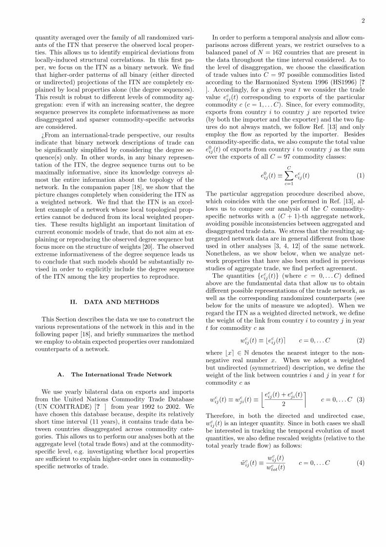
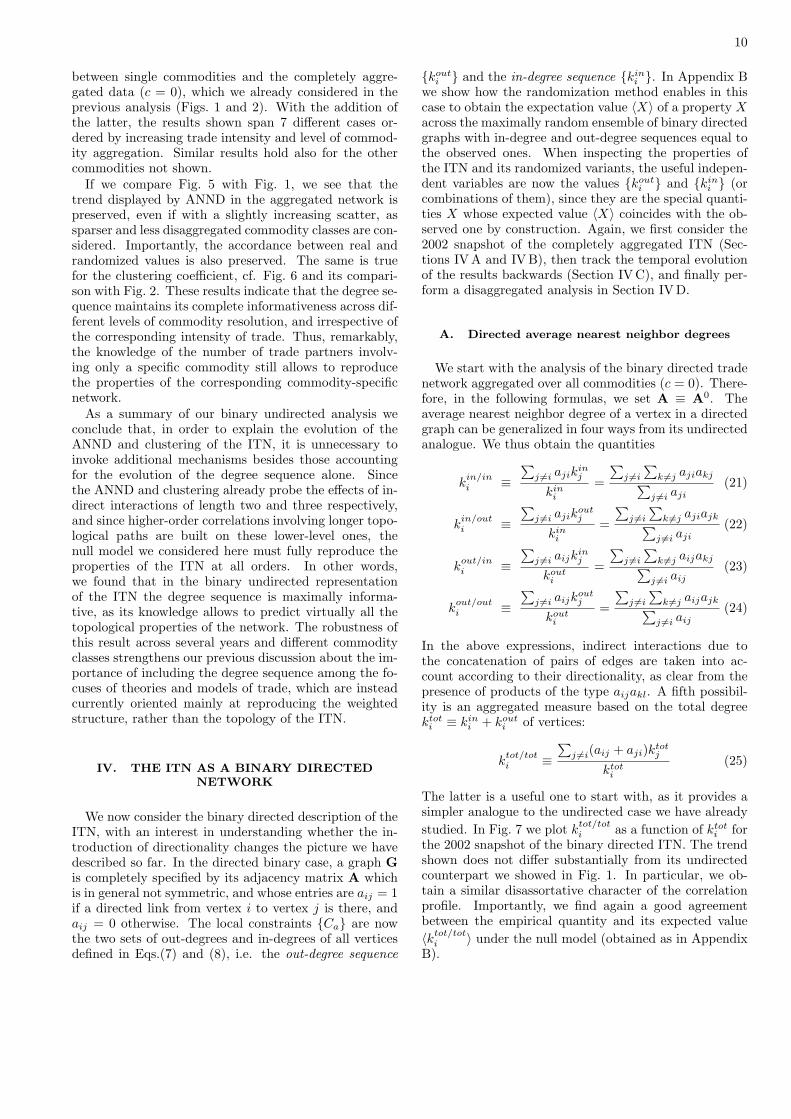
In Figs. 15 and 16 we show the behavior of the total av-erage nearest neighbor degree and total clustering coeffi-cient for the 2002 snapshots of the 6 selected commodity-specific networks. When compared with Figs. 7 and 9,the plots confirm what we have found in Section IIIDfor the binary undirected case. In particular, the be-havior displayed by the ANND and clustering in thecommodity-specific networks becomes less and less noisyas more intensely traded commodities, and higher levelsof aggregation, are considered. Accordingly, the agree-ment between real and randomized networks increases,but the accordance is already remarkable in commodity-specific networks, even the sparsest and least aggregatedones. These results confirm that, irrespective of the levelof commodity resolution and trade volume, the directeddegree sequences completely characterize the topology ofthe binary directed representations of the ITN.
0 20 40 60 80 100 120 1400.0
0.2
0.4
0.6
0.8
ktot
ctot ,X
ctot \
a
0 50 100 150 2000.0
0.2
0.4
0.6
0.8
ktot
ctot ,X
ctot \
b
0 50 100 150 200 2500.0
0.2
0.4
0.6
0.8
ktot
ctot ,X
ctot \
c
0 50 100 150 200 2500.0
0.2
0.4
0.6
0.8
1.0
ktot
ctot ,X
ctot \
d
0 50 100 150 200 2500.0
0.2
0.4
0.6
0.8
ktot
ctot ,X
ctot \
e
0 50 100 150 200 2500.0
0.2
0.4
0.6
0.8
1.0
ktot
ctot ,X
ctot \
f
FIG. 16: Total clustering coefficient ctoti versus total de-gree ktot
i in the 2002 snapshots of the commodity-specific(disaggregated) versions of the real binary directed ITN(red points), and corresponding average over the maximum-entropy ensemble with specified our-degrees and in-degrees(blue curve). a) commodity 93; b) commodity 09; c) com-modity 39; d) commodity 90; e) commodity 84; f) aggre-gation of the top 14 commodities (see Table I for details).From a) to f), the intensity of trade and level of aggregationincreases.
V. CONCLUSIONS
All the above results clearly imply that, in the undi-rected as well as the directed case, for all the years con-sidered, and across different commodity classes, the dis-assortativity and clustering profiles observed in the realbinary ITN arise as natural outcomes rather than gen-uine correlations, once the local topological propertiesare fixed to their observed values. Therefore we can con-clude that the higher-order patterns observed in all thebinary representations of the ITN, as well as their tem-poral evolution, are completely explained by local con-straints alone. This means that the degree sequence(s)of the ITN is maximally informative, since its knowl-edge systematically conveys a full picture of the binarytopology of the network. These results have importantconsequences for economic models of trade. In particu-lar, they suggest that the ITN topology should becomeone of the main focuses of international-trade theories.While most of the literature concerned with modelinginternational trade has focused on the problem of repro-ducing the magnitude of nonzero trade volumes (the most
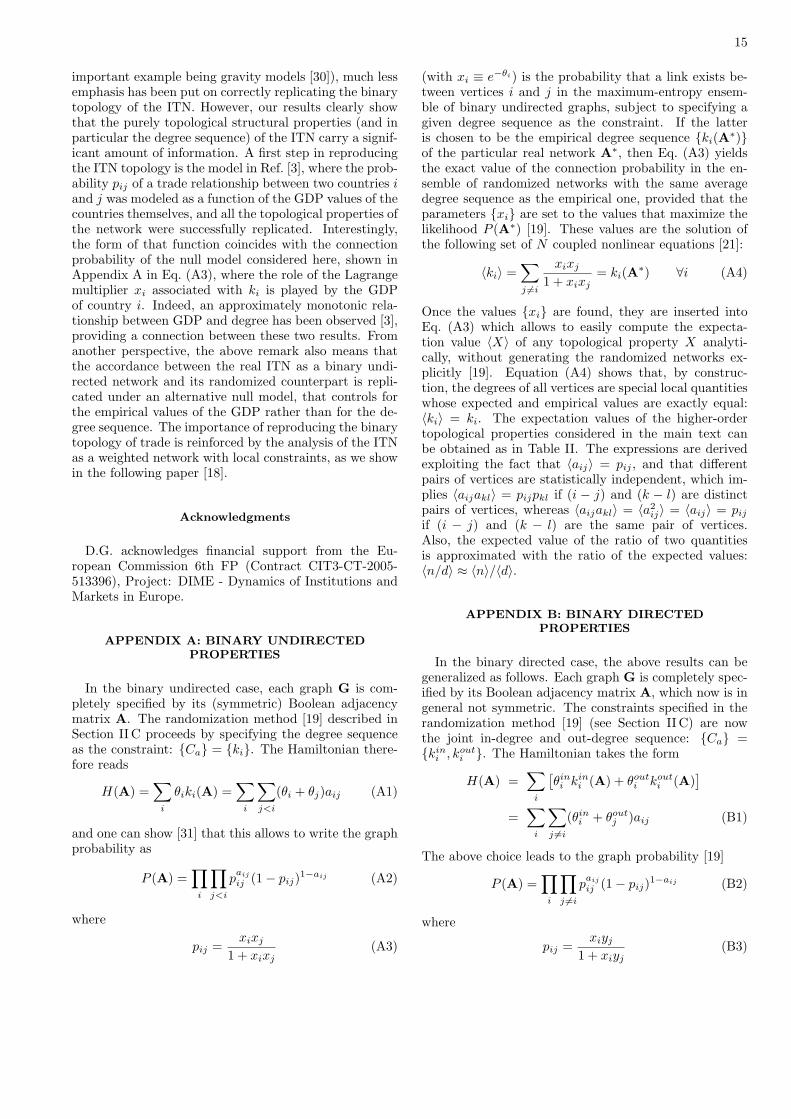
15
important example being gravity models [30]), much lessemphasis has been put on correctly replicating the binarytopology of the ITN. However, our results clearly showthat the purely topological structural properties (and inparticular the degree sequence) of the ITN carry a signif-icant amount of information. A first step in reproducingthe ITN topology is the model in Ref. [3], where the prob-ability pij of a trade relationship between two countries iand j was modeled as a function of the GDP values of thecountries themselves, and all the topological properties ofthe network were successfully replicated. Interestingly,the form of that function coincides with the connectionprobability of the null model considered here, shown inAppendix A in Eq. (A3), where the role of the Lagrangemultiplier xi associated with ki is played by the GDPof country i. Indeed, an approximately monotonic rela-tionship between GDP and degree has been observed [3],providing a connection between these two results. Fromanother perspective, the above remark also means thatthe accordance between the real ITN as a binary undi-rected network and its randomized counterpart is repli-cated under an alternative null model, that controls forthe empirical values of the GDP rather than for the de-gree sequence. The importance of reproducing the binarytopology of trade is reinforced by the analysis of the ITNas a weighted network with local constraints, as we showin the following paper [18].
Acknowledgments
D.G. acknowledges financial support from the Eu-ropean Commission 6th FP (Contract CIT3-CT-2005-513396), Project: DIME - Dynamics of Institutions andMarkets in Europe.
APPENDIX A: BINARY UNDIRECTEDPROPERTIES
In the binary undirected case, each graph G is com-pletely specified by its (symmetric) Boolean adjacencymatrix A. The randomization method [19] described inSection IIC proceeds by specifying the degree sequenceas the constraint: {Ca} = {ki}. The Hamiltonian there-fore reads
H(A) =∑
i
θiki(A) =∑
i
∑
j<i
(θi + θj)aij (A1)
and one can show [31] that this allows to write the graphprobability as
P (A) =∏
i
∏
j<i
paij
ij (1− pij)1−aij (A2)
where
pij =xixj
1 + xixj(A3)
(with xi ≡ e−θi) is the probability that a link exists be-tween vertices i and j in the maximum-entropy ensem-ble of binary undirected graphs, subject to specifying agiven degree sequence as the constraint. If the latteris chosen to be the empirical degree sequence {ki(A
∗)}of the particular real network A
∗, then Eq. (A3) yieldsthe exact value of the connection probability in the en-semble of randomized networks with the same averagedegree sequence as the empirical one, provided that theparameters {xi} are set to the values that maximize thelikelihood P (A∗) [19]. These values are the solution ofthe following set of N coupled nonlinear equations [21]:
〈ki〉 =∑
j 6=i
xixj
1 + xixj= ki(A
∗) ∀i (A4)
Once the values {xi} are found, they are inserted intoEq. (A3) which allows to easily compute the expecta-tion value 〈X〉 of any topological property X analyti-cally, without generating the randomized networks ex-plicitly [19]. Equation (A4) shows that, by construc-tion, the degrees of all vertices are special local quantitieswhose expected and empirical values are exactly equal:〈ki〉 = ki. The expectation values of the higher-ordertopological properties considered in the main text canbe obtained as in Table II. The expressions are derivedexploiting the fact that 〈aij〉 = pij , and that differentpairs of vertices are statistically independent, which im-plies 〈aijakl〉 = pijpkl if (i − j) and (k − l) are distinctpairs of vertices, whereas 〈aijakl〉 = 〈a2ij〉 = 〈aij〉 = pijif (i − j) and (k − l) are the same pair of vertices.Also, the expected value of the ratio of two quantitiesis approximated with the ratio of the expected values:〈n/d〉 ≈ 〈n〉/〈d〉.
APPENDIX B: BINARY DIRECTEDPROPERTIES
In the binary directed case, the above results can begeneralized as follows. Each graph G is completely spec-ified by its Boolean adjacency matrix A, which now is ingeneral not symmetric. The constraints specified in therandomization method [19] (see Section IIC) are nowthe joint in-degree and out-degree sequence: {Ca} ={kini , kouti }. The Hamiltonian takes the form
H(A) =∑
i
[
θini kini (A) + θouti kouti (A)]
=∑
i
∑
j 6=i
(θini + θoutj )aij (B1)
The above choice leads to the graph probability [19]
P (A) =∏
i
∏
j 6=i
paij
ij (1− pij)1−aij (B2)
where
pij =xiyj
1 + xiyj(B3)
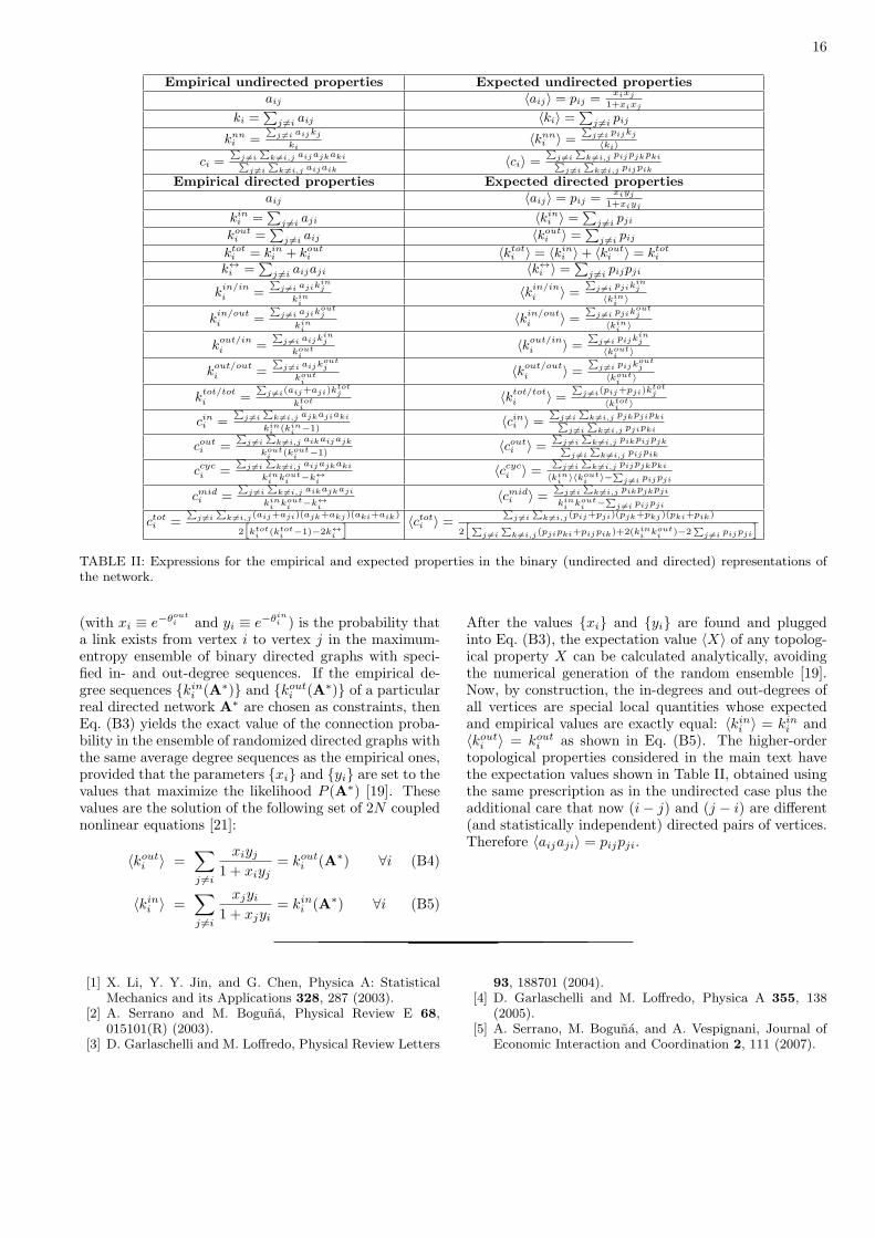
16
Empirical undirected properties Expected undirected propertiesaij 〈aij〉 = pij =
xixj
1+xixj
ki =∑
j 6=i aij 〈ki〉 =∑
j 6=i pij
knni =
∑j 6=i aijkj
ki〈knn
i 〉 =∑
j 6=i pijkj
〈ki〉
ci =∑
j 6=i
∑k 6=i,j aijajkaki∑
j 6=i
∑k 6=i,j aijaik
〈ci〉 =∑
j 6=i
∑k 6=i,j pijpjkpki∑
j 6=i
∑k 6=i,j pijpik
Empirical directed properties Expected directed propertiesaij 〈aij〉 = pij =
xiyj1+xiyj
kini =
∑
j 6=i aji 〈kini 〉 =
∑
j 6=i pji
kouti =
∑
j 6=i aij 〈kouti 〉 =
∑
j 6=i pij
ktoti = kin
i + kouti 〈ktot
i 〉 = 〈kini 〉+ 〈kout
i 〉 = ktoti
k↔i =
∑
j 6=i aijaji 〈k↔i 〉 =
∑
j 6=i pijpji
kin/ini =
∑j 6=i ajik
inj
kini
〈kin/ini 〉 =
∑j 6=i pjik
inj
〈kini
〉
kin/outi =
∑j 6=i ajik
outj
kini
〈kin/outi 〉 =
∑j 6=i pjik
outj
〈kini
〉
kout/ini =
∑j 6=i aijk
inj
kouti
〈kout/ini 〉 =
∑j 6=i pijk
inj
〈kouti
〉
kout/outi =
∑j 6=i aijk
outj
kouti
〈kout/outi 〉 =
∑j 6=i pijk
outj
〈kouti
〉
ktot/toti =
∑j 6=i(aij+aji)k
totj
ktoti
〈ktot/toti 〉 =
∑j 6=i(pij+pji)k
totj
〈ktoti
〉
cini =∑
j 6=i
∑k 6=i,j ajkajiaki
kini
(kini
−1)〈cini 〉 =
∑j 6=i
∑k 6=i,j pjkpjipki∑
j 6=i
∑k 6=i,j pjipki
couti =∑
j 6=i
∑k 6=i,j aikaijajk
kouti
(kouti
−1)〈couti 〉 =
∑j 6=i
∑k 6=i,j pikpijpjk∑
j 6=i
∑k 6=i,j pijpik
ccyci =
∑j 6=i
∑k 6=i,j aijajkaki
kini
kouti
−k↔i
〈ccyci 〉 =∑
j 6=i
∑k 6=i,j pijpjkpki
〈kini
〉〈kouti
〉−∑
j 6=i pijpji
cmidi =
∑j 6=i
∑k 6=i,j aikajkaji
kini
kouti
−k↔i
〈cmidi 〉 =
∑j 6=i
∑k 6=i,j pikpjkpji
kini
kouti
−∑
j 6=i pijpji
ctoti =∑
j 6=i
∑k 6=i,j(aij+aji)(ajk+akj)(aki+aik)
2[
ktoti
(ktoti
−1)−2k↔i
] 〈ctoti 〉 =∑
j 6=i
∑k 6=i,j(pij+pji)(pjk+pkj)(pki+pik)
2[∑
j 6=i
∑k 6=i,j(pjipki+pijpik)+2(kin
ikouti
)−2∑
j 6=i pijpji
]
TABLE II: Expressions for the empirical and expected properties in the binary (undirected and directed) representations ofthe network.
(with xi ≡ e−θouti and yi ≡ e−θin
i ) is the probability thata link exists from vertex i to vertex j in the maximum-entropy ensemble of binary directed graphs with speci-fied in- and out-degree sequences. If the empirical de-gree sequences {kini (A∗)} and {kouti (A∗)} of a particularreal directed network A
∗ are chosen as constraints, thenEq. (B3) yields the exact value of the connection proba-bility in the ensemble of randomized directed graphs withthe same average degree sequences as the empirical ones,provided that the parameters {xi} and {yi} are set to thevalues that maximize the likelihood P (A∗) [19]. Thesevalues are the solution of the following set of 2N couplednonlinear equations [21]:
〈kouti 〉 =∑
j 6=i
xiyj1 + xiyj
= kouti (A∗) ∀i (B4)
〈kini 〉 =∑
j 6=i
xjyi1 + xjyi
= kini (A∗) ∀i (B5)
After the values {xi} and {yi} are found and pluggedinto Eq. (B3), the expectation value 〈X〉 of any topolog-ical property X can be calculated analytically, avoidingthe numerical generation of the random ensemble [19].Now, by construction, the in-degrees and out-degrees ofall vertices are special local quantities whose expectedand empirical values are exactly equal: 〈kini 〉 = kini and〈kouti 〉 = kouti as shown in Eq. (B5). The higher-ordertopological properties considered in the main text havethe expectation values shown in Table II, obtained usingthe same prescription as in the undirected case plus theadditional care that now (i− j) and (j − i) are different(and statistically independent) directed pairs of vertices.Therefore 〈aijaji〉 = pijpji.
[1] X. Li, Y. Y. Jin, and G. Chen, Physica A: StatisticalMechanics and its Applications 328, 287 (2003).
[2] A. Serrano and M. Boguna, Physical Review E 68,015101(R) (2003).
[3] D. Garlaschelli and M. Loffredo, Physical Review Letters
93, 188701 (2004).[4] D. Garlaschelli and M. Loffredo, Physica A 355, 138
(2005).[5] A. Serrano, M. Boguna, and A. Vespignani, Journal of
Economic Interaction and Coordination 2, 111 (2007).

17
[6] K. Bhattacharya, G. Mukherjee, J. Saramaki, K. Kaski,and S. Manna, Journal of Statistical Mechanics: TheoryExp. A 2, P02002 (2008).
[7] K. Bhattacharya, G. Mukherjee, and S. Manna, inEconophysics of Markets and Business Networks, editedby A. Chatterjee and B. Chakrabarti (Springer-Verlag,Milan, Italy, 2007).
[8] D. Garlaschelli, T. Di Matteo, T. Aste, G. Caldarelli, andM. Loffredo, The European Physical Journal B 57, 1434(2007).
[9] I. Tzekina, K. Danthi, and D. Rockmore, The EuropeanPhysical Journal B - Condensed Matter 63, 541 (2008).
[10] G. Fagiolo, S. Schiavo, and J. Reyes, Physica A 387, 3868(2008).
[11] J. Reyes, S. Schiavo, and G. Fagiolo, Advances in Com-plex Systems 11, 685 (2008).
[12] G. Fagiolo, S. Schiavo, and J. Reyes, Physical Review E79, 036115 (2009).
[13] M. Barigozzi, G. Fagiolo, and D. Garlaschelli, PhysicalReview E 81, 046104 (2010).
[14] G. Caldarelli, Scale-free networks: complex webs in na-ture and technology (Oxford Univ. Press, Oxford, 2007).
[15] R. Albert and A.-L. Barabasi, Reviews of ModernPhysics 74, 47 (2002).
[16] S. Dorogovtsev and J. Mendes, Evolution of Networks:From Biological Nets to the Internet and WWW (Oxford,Oxford University Press, 2003).
[17] R. Feenstra, Advanced international trade : theory andevidence (Princeton University Press, 2004).
[18] T. Squartini, G. Fagiolo, and D. Garlaschelli, LEM WPSeries 2011–09, Laboratory of Economics and Manage-ment (LEM) (2011).
[19] T. Squartini and D. Garlaschelli, PreprintarXiv:1103.0701v1 [physics.data-an] (2011).
[20] P. van Bergeijk and S. Brakman, eds., The Gravity Modelin International Trade (Cambridge University Press,Cambridge, 2010).
[21] D. Garlaschelli and M. I. Loffredo, Physical Review E78, 015101 (2008).
[22] M. A. Serrano, Physical Review E 78, 026101 (2008).[23] D. Garlaschelli and M. I. Loffredo, Physical Review Let-
ters 93, 268701 (2004).[24] S. Maslov and K. Sneppen, Science 296, 910 (2002).[25] Physica A: Statistical and Theoretical Physics 333, 529
(2004).[26] J. Park and M. E. J. Newman, Physical Review E 68,
026112 (2003).[27] R. Pastor-Satorras, A. Vazquez, and A. Vespignani,
Physical Review Letters 87, 258701 (2001).[28] G. Fagiolo, Physical Review E 76, 026107 (2007).[29] R. Milo, S. Shen-Orr, S. Itzkovitz, N. Kashtan,
D. Chklovskii, and U. Alon, Science 298, 824 (2002).[30] G. Fagiolo, Journal of Economic Interaction and Coordi-
nation 5, 1 (2010).[31] J. Park and M. E. J. Newman, Physical Review E 70,
066117 (2004).[32] http://comtrade.un.org/.[33] http://unstats.un.org/.[34] We left {e9ij(t)} and {e93ij (t)} in current U.S. dollars
(USD); we divided {e39ij (t)} and {e90ij (t)} by 10; we di-
vided {e84ij (t)} and the sum of the top 14 commodities
by 100; we divided aggregate data ({e0ij(t)}) by 1000.Accordingly, after the rounding defined by eqs.(2) and(3), we obtained trade flows {wc
ij(t)} expressed in inte-ger multiples of either 1 USD, 10 USD, 100 USD, or 1000USD.