Reward-to-Risk Ratios of Fund of Hedge Funds

YIGIT ATILGAN

Assistant Professor of Finance, Sabanci University

TURAN G. BALI

Dean’s Research Professor of Finance, Georgetown University

K. OZGUR DEMIRTAS

Associate Professor of Finance, Baruch College, CUNY, and Sabanci University

ABSTRACT

This chapter examines whether the fund of hedge fund portfolios dominate the U.S. equity and bond markets based on alternative measures of reward-to-risk ratios. Standard deviation is used to measure total risk and both nonparametric and parametric value-at-risk is used to measure downside risk when the reward-to-risk ratios are constructed. We find that the fund of funds index has higher reward-to-risk ratios compared to several stock and bond market indices. This result is especially strong when the risk measures are calculated from the most recent year’s data and is robust as the measurement window is extended to four years.

2

1. INTRODUCTION

Investors base their portfolio asset allocation decisions on the interactions between risks

and returns of available financial securities. The assumption of risk aversion implies that

securities with greater risk should demand greater return. Although the trade-off between

risk and return is well-established in financial economics, the ability to generate higher

expected returns per unit risk can vary from one security to another. This chapter

compares various reward-to-risk ratios for the Fund of Hedge Fund (FoHF) index with

those of several bond and stock market indices.

Traditional risk measures used in portfolio performance measurement assume that returns

are normally distributed and therefore the standard deviation of the empirical return

distribution is a good estimate of risk only if the underlying return distribution is close to

normal. The first measure of reward-to-risk that we use is the Sharpe ratio (1966) which

is equal to the ratio of the mean excess return of a portfolio to its standard deviation. The

Sharpe ratio is the most common measure of how well the return of a portfolio

compensates the investor for the risk taken. However, a common criticism is that it is too

broad since it includes the total risk of a portfolio in its denominator. Another potential

issue regarding the calculation of Sharpe ratios for the FoHF index is the non-normality

of hedge fund return distributions.

The hedge fund literature provides evidence that distributions of hedge fund returns tend

to deviate from normality. Malkiel and Saha (2005) report that the distribution of hedge

3

fund returns generally have high kurtosis and negative skewness. The documented

deviation from normality can be traced to the unique investment strategies that hedge

funds follow. Fung and Hsieh (1997) observe that hedge fund managers are flexible to

choose among a diverse set of asset classes and they can use dynamic trading strategies

that involve short sales, leverage and derivatives. Such strategies have the potential to

induce option-like payouts and exposure to tail events for hedge funds. In a follow-up

study, Fung and Hsieh (2001) focus on hedge funds that use trend-following strategies.

They construct several trend-following factors that can replicate key features of hedge

fund returns such as skewness and positive returns during extreme market movements.

Mitchell and Pulvino (2001) investigate merger arbitrage strategies and conjecture that

returns to risk arbitrage are related to market returns in a nonlinear way. Their results

indicate that merger risk arbitrage is similar to writing uncovered index put options.

Agarwal and Naik (2004) find that nonlinear payoff structures exist for a wide range of

hedge fund strategies including equity-oriented positions. They state that ignoring the

downside risk of hedge funds can result in significantly higher losses during large market

downturns. Brown, Gregoriou and Pascalau (2009) look at the diversification effect of

investing in FoHFs and find that the magnitude of skewness is an increasing function of

diversification offered by FoHFs. Their finding suggests that downside risk exposure may

not be diversifiable. Finally, Bali, Gokcan and Liang (2007) and Liang and Park (2007)

provide direct evidence that downside risk measures such as value-at-risk, expected

shortfall and tail risk can explain the cross-section of hedge fund returns.

4

Downside risk is a function of the higher order moments of a return distribution and even

without the existence of nonlinear payoffs, higher order moments such as skewness and

kurtosis have been found to play an important role in asset pricing. The mean-variance

portfolio theory of Markowitz (1952) has been extended by Arditti (1967) and Kraus and

Litzenberger (1976) to incorporate the effect of skewness. These studies present three-

moment asset pricing models with investors that hold concave preferences and prefer

positive skewness. The main implication of these models is that assets that increase a

portfolio’s skewness are more desirable and should command lower expected returns.

Harvey and Siddique (2000) extend these unconditional pricing models and incorporate

conditional co-skewness. Again, the implication is that risk-averse investors prefer

positively skewed assets to negatively skewed assets. As far as the fourth-moment is

concerned, Dittmar (2002) builds on the theoretical works of Kimball (1993) and Pratt

and Zeckhauser (1987) and finds preference for lower kurtosis. Asset distributions with

lower probability mass in their tails are preferred and therefore assets that increase a

portfolio’s kurtosis are less desirable and should command higher expected returns.

Downside risk increases with kurtosis and decreases with skewness (Cornish and Fisher

(1937)). Given the importance of these return moments for asset pricing and the

prevalence of downside risk in hedge fund returns, we place special emphasis on the

concept of downside risk in our reward-to-risk analysis. To investigate how much

expected return each index commands per unit of downside risk, we use both a

nonparametric and parametric measure of value-at-risk in the construction of the

alternative reward-to-risk ratios. For the nonparametric VaRSharpe ratio, the

5

denominator is the absolute value of the minimum index return over various past sample

windows. For the parametric reward-to-downside risk measure (PVaRSharpe), the

denominator is based on the lower tail of Hansen’s (1994) skewed t-density.

The results indicate that the FoHF index outperforms the bond and stock market indices

based on traditional Sharpe ratios on average. Although the Sharpe ratios decrease for

every index as the sampling window for the calculation of standard deviation is extended

and this decline is most pronounced for the FoHF index, it has the highest Sharpe ratio

regardless of the sampling window. When we take downside risk into account through

nonparametric and parametric value-at-risk, the results are similar. The FoHF index has

higher downside risk-adjusted Sharpe ratios compared to all bond and stock market

indices and this result is especially strong at shorter sampling windows for value-at-risk

measurement.

The chapter is organized as follows. Section 2 discusses the methodology for calculating

the reward-to-risk ratios. Section 3 explains the data and presents the summary statistics.

Section 4 discusses the empirical results. Section 5 concludes.

2. METHODOLOGY

We estimate three reward-to-risk ratios that differ from each other based on the risk

measure used in the denominator. The first of these ratios is the standard Sharpe ratio:

6

ti

tfti

tiStDev

RRSharpe

,

,,

,

−= (1)

where Ri,t denotes the month t return on the fund of funds, bond or stock market index i

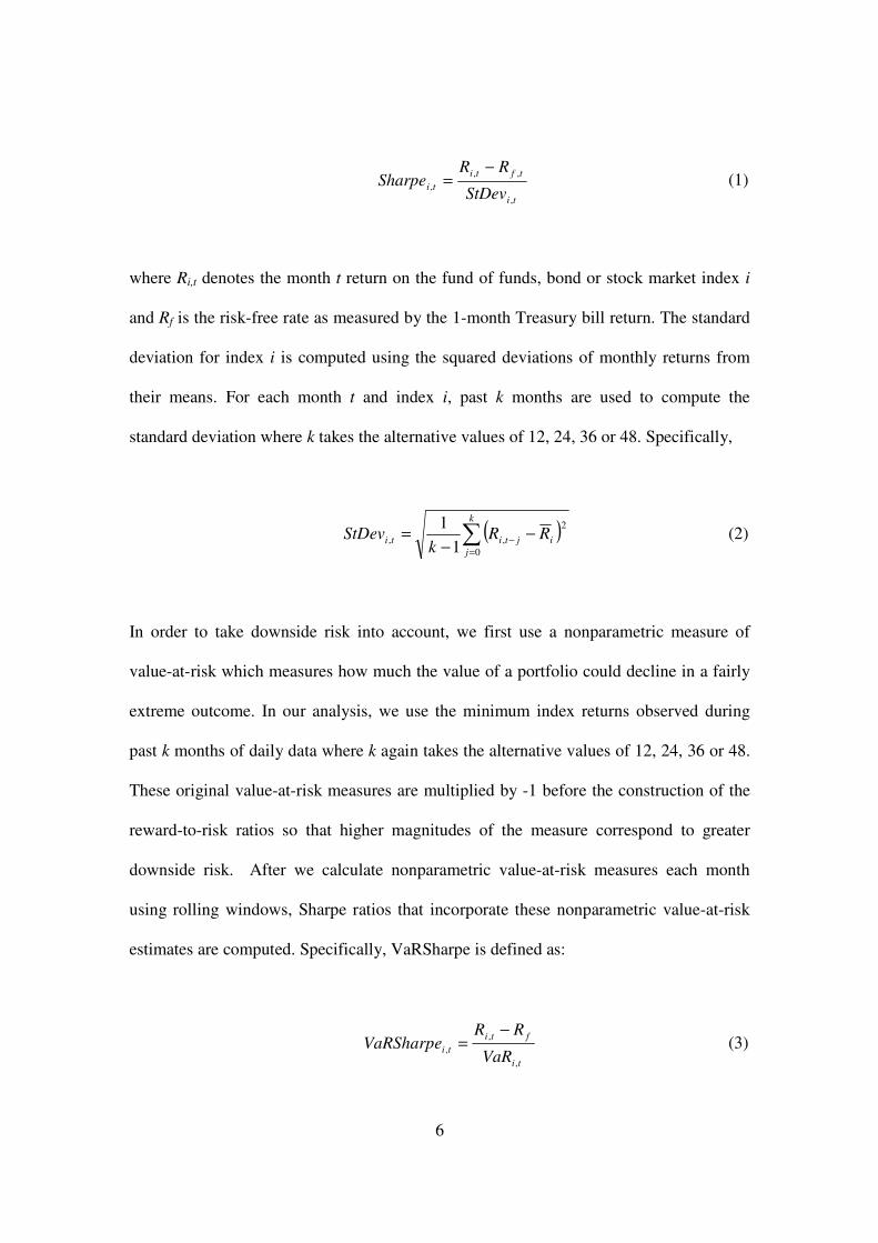
and Rf is the risk-free rate as measured by the 1-month Treasury bill return. The standard

deviation for index i is computed using the squared deviations of monthly returns from

their means. For each month t and index i, past k months are used to compute the

standard deviation where k takes the alternative values of 12, 24, 36 or 48. Specifically,

( )∑=

− −−

=k

j

ijtiti RRk

StDev0

2

,,1

1 (2)

In order to take downside risk into account, we first use a nonparametric measure of

value-at-risk which measures how much the value of a portfolio could decline in a fairly

extreme outcome. In our analysis, we use the minimum index returns observed during

past k months of daily data where k again takes the alternative values of 12, 24, 36 or 48.

These original value-at-risk measures are multiplied by -1 before the construction of the

reward-to-risk ratios so that higher magnitudes of the measure correspond to greater

downside risk. After we calculate nonparametric value-at-risk measures each month

using rolling windows, Sharpe ratios that incorporate these nonparametric value-at-risk

estimates are computed. Specifically, VaRSharpe is defined as:

ti

fti

tiVaR

RRVaRSharpe

,

,

,

−= (3)

7

where VaRi,t is the nonparametric value at risk.

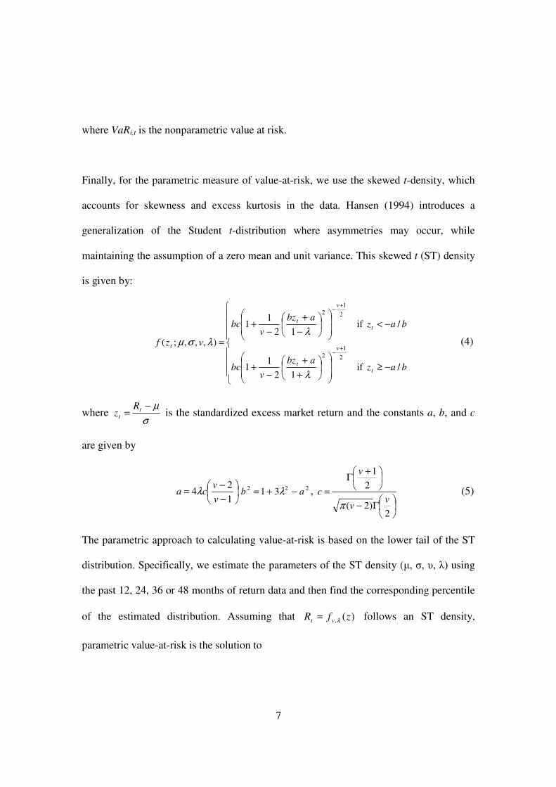
Finally, for the parametric measure of value-at-risk, we use the skewed t-density, which

accounts for skewness and excess kurtosis in the data. Hansen (1994) introduces a

generalization of the Student t-distribution where asymmetries may occur, while

maintaining the assumption of a zero mean and unit variance. This skewed t (ST) density

is given by:

−≥

+

+

−+

−<

−

+

−+

=+

−

+−

bazabz

vbc

bazabz

vbc

vzf

t

v

t

t

v

t

t

/ if 12

11

/ if 12

11

),,,;(

2

12

2

12

λ

λλσµ

(4)

where σ

µ−= t

t

Rz is the standardized excess market return and the constants a, b, and c

are given by

−

−=

1

24

v

vca λ 222 31 ab −+= λ ,

Γ−

+Γ

=

2)2(

2

1

vv

v

c

π

(5)

The parametric approach to calculating value-at-risk is based on the lower tail of the ST

distribution. Specifically, we estimate the parameters of the ST density (µ, σ, υ, λ) using

the past 12, 24, 36 or 48 months of return data and then find the corresponding percentile

of the estimated distribution. Assuming that )(, zfR vt λ= follows an ST density,

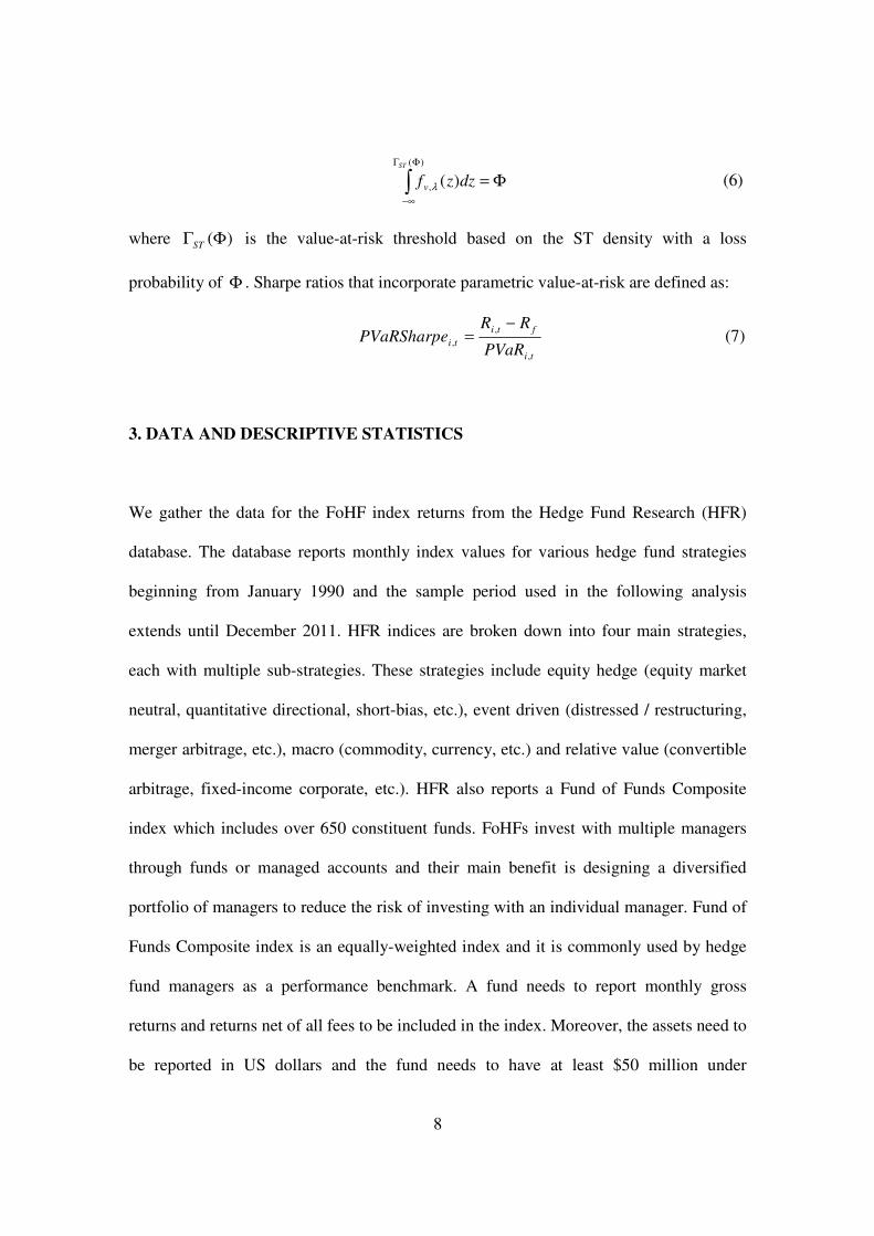
parametric value-at-risk is the solution to

8

∫ΦΓ

∞−

Φ=

)(

, )(ST

dzzfv λ (6)

where )(ΦΓST is the value-at-risk threshold based on the ST density with a loss

probability of Φ . Sharpe ratios that incorporate parametric value-at-risk are defined as:

ti

fti

tiPVaR

RRPVaRSharpe

,

,

,

−= (7)

3. DATA AND DESCRIPTIVE STATISTICS

We gather the data for the FoHF index returns from the Hedge Fund Research (HFR)

database. The database reports monthly index values for various hedge fund strategies

beginning from January 1990 and the sample period used in the following analysis

extends until December 2011. HFR indices are broken down into four main strategies,

each with multiple sub-strategies. These strategies include equity hedge (equity market

neutral, quantitative directional, short-bias, etc.), event driven (distressed / restructuring,

merger arbitrage, etc.), macro (commodity, currency, etc.) and relative value (convertible

arbitrage, fixed-income corporate, etc.). HFR also reports a Fund of Funds Composite

index which includes over 650 constituent funds. FoHFs invest with multiple managers

through funds or managed accounts and their main benefit is designing a diversified

portfolio of managers to reduce the risk of investing with an individual manager. Fund of

Funds Composite index is an equally-weighted index and it is commonly used by hedge

fund managers as a performance benchmark. A fund needs to report monthly gross

returns and returns net of all fees to be included in the index. Moreover, the assets need to

be reported in US dollars and the fund needs to have at least $50 million under

9

management or have been actively trading for at least twelve months. Funds are included

in the composite index the month after their addition to the database.

We also collect data for various bond and stock market indices for comparison purposes.

Specifically, we collect price data for indices that track Treasury bonds with maturities of

5, 10, 20 and 30 years. For equities, we focus on the S&P 500 index and the

NYSE/AMEX/NASDAQ index with distributions. All the data for the bond and stock

market indices come from the Center for Research in Security Prices (CRSP). The yield

for the 1-month Treasury bill which is used to proxy for the risk-free rate is downloaded

from Kenneth French’s online data library.

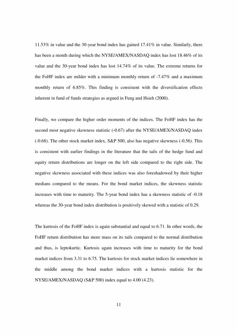
Table 1 reports the descriptive statistics for all indices. A comparison of means shows

that the NYSE/AMEX/NASDAQ index has the highest monthly return (0.78%), however

the S&P 500 index has not generated as high an average return (0.58%). This difference

can be explained by the greater returns generated by small stocks historically. The mean

returns on the bond indices increase by time to maturity with the 5-year bond index

delivering 0.56% per month and the 30-year bond index delivering 0.73% per month. In

terms of means, the FoHF index sits somewhere in the middle in this picture with a

monthly mean return of 0.61%. The medians tell a similar story with the biggest

difference being that both stock market indices have generated higher median returns

than all other indices. NYSE/AMEX/NASDAQ index had a median return of 1.34% over

the sample period whereas S&P 500 index had a median return of 1.01%. Again, the

10

median returns for the bond indices increase by time to maturity and vary from 0.58% to

0.89%. The FoHF index still positions itself in the middle with a median return of 0.77%.

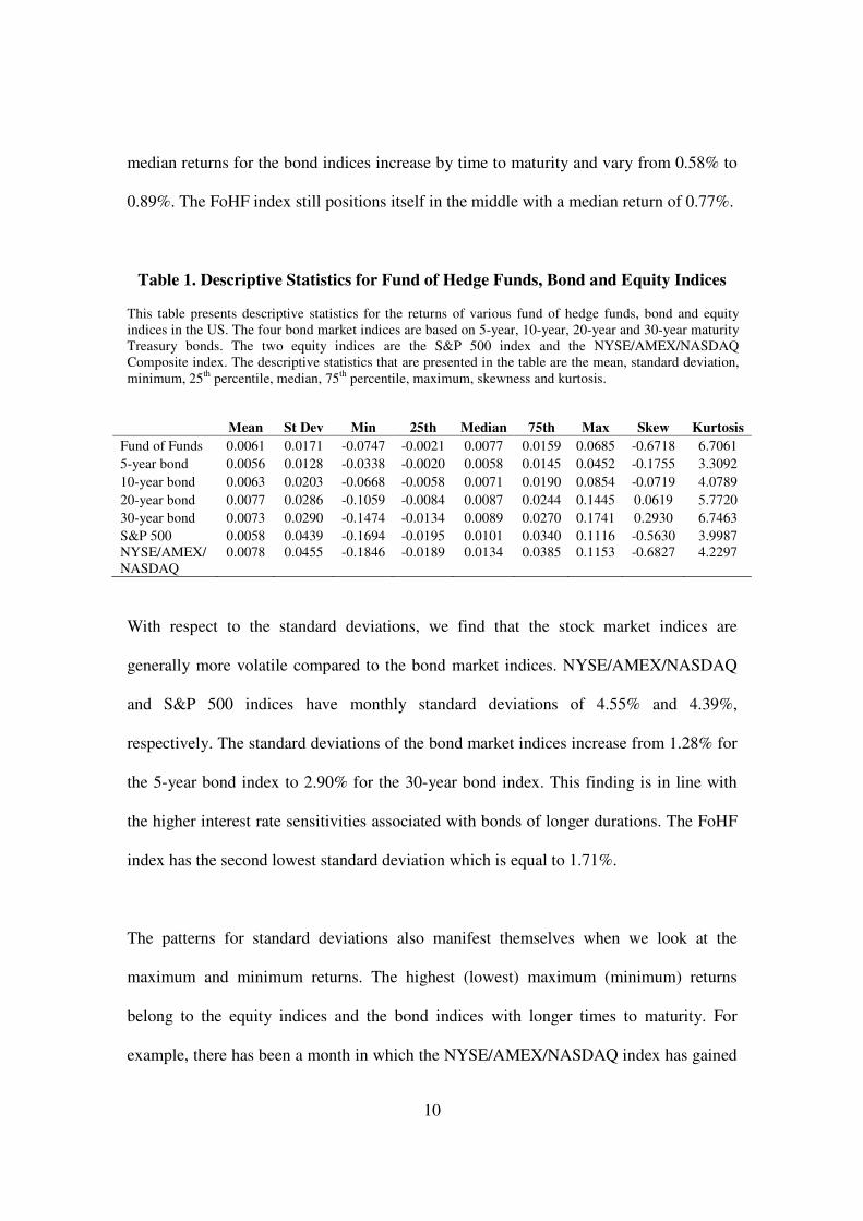
Table 1. Descriptive Statistics for Fund of Hedge Funds, Bond and Equity Indices

This table presents descriptive statistics for the returns of various fund of hedge funds, bond and equity indices in the US. The four bond market indices are based on 5-year, 10-year, 20-year and 30-year maturity Treasury bonds. The two equity indices are the S&P 500 index and the NYSE/AMEX/NASDAQ Composite index. The descriptive statistics that are presented in the table are the mean, standard deviation, minimum, 25th percentile, median, 75th percentile, maximum, skewness and kurtosis.

Mean St Dev Min 25th Median 75th Max Skew Kurtosis

Fund of Funds 0.0061 0.0171 -0.0747 -0.0021 0.0077 0.0159 0.0685 -0.6718 6.7061

5-year bond 0.0056 0.0128 -0.0338 -0.0020 0.0058 0.0145 0.0452 -0.1755 3.3092

10-year bond 0.0063 0.0203 -0.0668 -0.0058 0.0071 0.0190 0.0854 -0.0719 4.0789

20-year bond 0.0077 0.0286 -0.1059 -0.0084 0.0087 0.0244 0.1445 0.0619 5.7720

30-year bond 0.0073 0.0290 -0.1474 -0.0134 0.0089 0.0270 0.1741 0.2930 6.7463

S&P 500 0.0058 0.0439 -0.1694 -0.0195 0.0101 0.0340 0.1116 -0.5630 3.9987 NYSE/AMEX/ NASDAQ

0.0078 0.0455 -0.1846 -0.0189 0.0134 0.0385 0.1153 -0.6827 4.2297

With respect to the standard deviations, we find that the stock market indices are

generally more volatile compared to the bond market indices. NYSE/AMEX/NASDAQ

and S&P 500 indices have monthly standard deviations of 4.55% and 4.39%,

respectively. The standard deviations of the bond market indices increase from 1.28% for

the 5-year bond index to 2.90% for the 30-year bond index. This finding is in line with

the higher interest rate sensitivities associated with bonds of longer durations. The FoHF

index has the second lowest standard deviation which is equal to 1.71%.

The patterns for standard deviations also manifest themselves when we look at the

maximum and minimum returns. The highest (lowest) maximum (minimum) returns

belong to the equity indices and the bond indices with longer times to maturity. For

example, there has been a month in which the NYSE/AMEX/NASDAQ index has gained

11

11.53% in value and the 30-year bond index has gained 17.41% in value. Similarly, there

has been a month during which the NYSE/AMEX/NASDAQ index has lost 18.46% of its

value and the 30-year bond index has lost 14.74% of its value. The extreme returns for

the FoHF index are milder with a minimum monthly return of -7.47% and a maximum

monthly return of 6.85%. This finding is consistent with the diversification effects

inherent in fund of funds strategies as argued in Fung and Hsieh (2000).

Finally, we compare the higher order moments of the indices. The FoHF index has the

second most negative skewness statistic (-0.67) after the NYSE/AMEX/NASDAQ index

(-0.68). The other stock market index, S&P 500, also has negative skewness (-0.56). This

is consistent with earlier findings in the literature that the tails of the hedge fund and

equity return distributions are longer on the left side compared to the right side. The

negative skewness associated with these indices was also foreshadowed by their higher

medians compared to the means. For the bond market indices, the skewness statistic

increases with time to maturity. The 5-year bond index has a skewness statistic of -0.18

whereas the 30-year bond index distribution is positively skewed with a statistic of 0.29.

The kurtosis of the FoHF index is again substantial and equal to 6.71. In other words, the

FoHF return distribution has more mass on its tails compared to the normal distribution

and thus, is leptokurtic. Kurtosis again increases with time to maturity for the bond

market indices from 3.31 to 6.75. The kurtosis for stock market indices lie somewhere in

the middle among the bond market indices with a kurtosis statistic for the

NYSE/AMEX/NASDAQ (S&P 500) index equal to 4.00 (4.23).

12

4. EMPIRICAL RESULTS

Table 2 presents the traditional Sharpe ratios that incorporate the standard deviation of a

portfolio in its denominator. We calculate these monthly Sharpe ratios in a rolling

window fashion and use different sampling windows to calculate the standard deviations.

The length of the sampling windows ranges from 12 to 48 months. We present both the

time-series mean and the standard deviations of the reward-to-risk ratios for all indices.

Table 2. Standard Deviation-Based Sharpe Ratios for Fund of Hedge Funds,

Bond and Equity Indices

This table presents the standard deviation-based Sharpe ratios for various fund of hedge funds, bond and equity indices in the US. The four bond market indices are based on 5-year, 10-year, 20-year and 30-year maturity Treasury bonds. The two equity indices are the S&P 500 index and the NYSE/AMEX/NASDAQ Composite index. The numerator of the standard deviation-based Sharpe ratio is equal to the monthly return of the index minus the risk-free rate. The denominator is equal to the standard deviation of monthly returns over the past 12, 24, 36 or 48 months. Each row reports the means of each ratio and the standard deviations are presented in parentheses.

Sharpe12 Sharpe24 Sharpe36 Sharpe48

Fund of Funds 0.3516 (0.5182) 0.2979 (0.3166) 0.2629 (0.2363) 0.2357 (0.1517)

5-year bond 0.2223 (0.3709) 0.2127 (0.2823) 0.2088 (0.2338) 0.2037 (0.1857)

10-year bond 0.1801 (0.3278) 0.1676 (0.2080) 0.1630 (0.1592) 0.1561 (0.1123)

20-year bond 0.1949 (0.3024) 0.1766 (0.1639) 0.1724 (0.1204) 0.1674 (0.0821)

30-year bond 0.1397 (0.3072) 0.1252 (0.1576) 0.1231 (0.1119) 0.1179 (0.0744)

SP500 0.1653 (0.3601) 0.1292 (0.2472) 0.1104 (0.1988) 0.1054 (0.1719) NYSE/AMEX/ NASDAQ

0.2324 (0.3703) 0.1904 (0.2443) 0.1679 (0.1967) 0.1583 (0.1656)

When the standard deviation is calculated from the most recent year’s data, the FoHF

index generates the highest excess return per unit risk. The Sharpe ratio for FoHF is equal

to 0.352 which implies that the index demands extra 35 basis points of expected return

per 1% increase in standard deviation. The comparison between the bond and stock

13

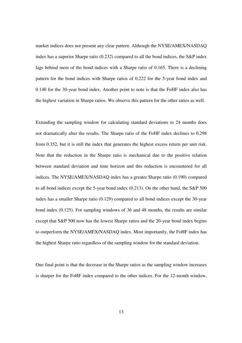
market indices does not present any clear pattern. Although the NYSE/AMEX/NASDAQ

index has a superior Sharpe ratio (0.232) compared to all the bond indices, the S&P index

lags behind most of the bond indices with a Sharpe ratio of 0.165. There is a declining

pattern for the bond indices with Sharpe ratios of 0.222 for the 5-year bond index and

0.140 for the 30-year bond index. Another point to note is that the FoHF index also has

the highest variation in Sharpe ratios. We observe this pattern for the other ratios as well.

Extending the sampling window for calculating standard deviations to 24 months does

not dramatically alter the results. The Sharpe ratio of the FoHF index declines to 0.298

from 0.352, but it is still the index that generates the highest excess return per unit risk.

Note that the reduction in the Sharpe ratio is mechanical due to the positive relation

between standard deviation and time horizon and this reduction is encountered for all

indices. The NYSE/AMEX/NASDAQ index has a greater Sharpe ratio (0.190) compared

to all bond indices except the 5-year bond index (0.213). On the other hand, the S&P 500

index has a smaller Sharpe ratio (0.129) compared to all bond indices except the 30-year

bond index (0.125). For sampling windows of 36 and 48 months, the results are similar

except that S&P 500 now has the lowest Sharpe ratios and the 20-year bond index begins

to outperform the NYSE/AMEX/NASDAQ index. Most importantly, the FoHF index has

the highest Sharpe ratio regardless of the sampling window for the standard deviation.

One final point is that the decrease in the Sharpe ratios as the sampling window increases

is sharper for the FoHF index compared to the other indices. For the 12-month window,

14

the Sharpe ratio of the FoHF index exceeds its closest follower by 0.120 (0.352 vs. 0.232)

whereas the difference is reduced to 0.038 (0.236 vs. 0.204) for the 48-month window.

These results collectively suggest that the FoHF index generates a higher excess return

per unit risk when risk is measured by standard deviation. However, there is enough

evidence in the literature to believe that the standard deviation is an incomplete measure

of risk for hedge fund returns whose distribution deviates from normality. This is also

evidenced by the negatively skewed and leptokurtic behavior of the FoHF index returns

in Table 1. Therefore, to take the nonlinearities hedge fund returns into account, we

calculate alternative Sharpe ratios based on nonparametric and parametric value-at-risk.

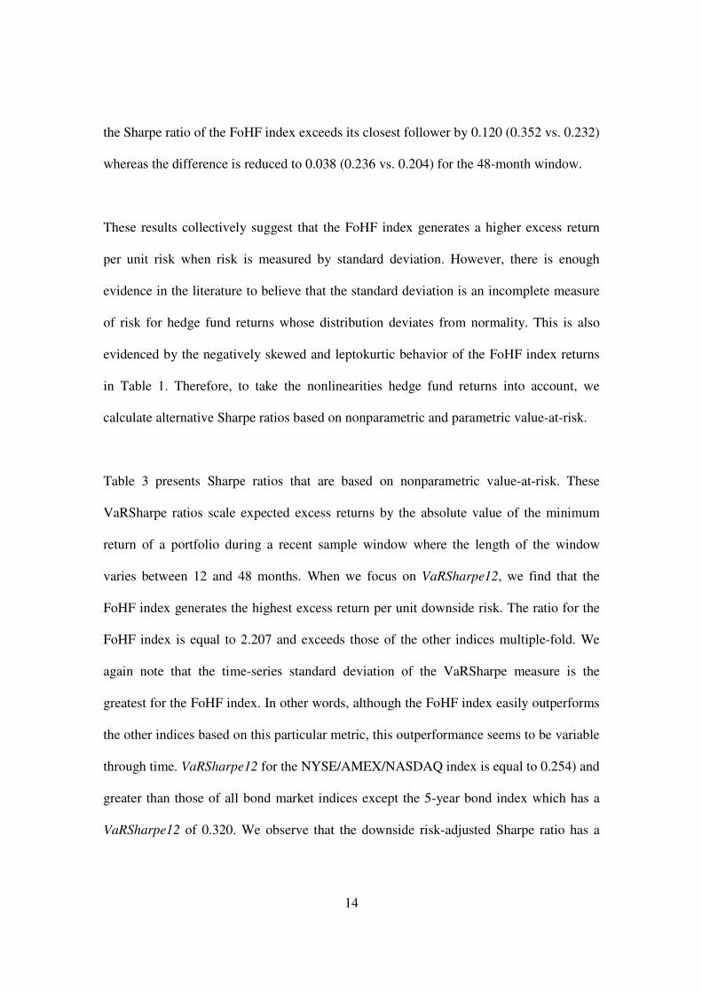
Table 3 presents Sharpe ratios that are based on nonparametric value-at-risk. These

VaRSharpe ratios scale expected excess returns by the absolute value of the minimum

return of a portfolio during a recent sample window where the length of the window

varies between 12 and 48 months. When we focus on VaRSharpe12, we find that the

FoHF index generates the highest excess return per unit downside risk. The ratio for the

FoHF index is equal to 2.207 and exceeds those of the other indices multiple-fold. We

again note that the time-series standard deviation of the VaRSharpe measure is the

greatest for the FoHF index. In other words, although the FoHF index easily outperforms

the other indices based on this particular metric, this outperformance seems to be variable

through time. VaRSharpe12 for the NYSE/AMEX/NASDAQ index is equal to 0.254) and

greater than those of all bond market indices except the 5-year bond index which has a

VaRSharpe12 of 0.320. We observe that the downside risk-adjusted Sharpe ratio has a

15

declining pattern for the bond market indices as the time to maturity increases and the 30-

year bond index has a VaRSharpe12 of 0.239. The S&P 500 index has a similar

performance with a VaRSharpe12 of 0.245. To summarize, the FoHF index is the

superior performer based on VaRSharpe12 and neither the bond nor the stock market

indices clearly dominate each other.

Table 3. Nonparametric Value at Risk-Based Sharpe Ratios for

Fund of Hedge Funds, Bond and Equity Indices

This table presents the nonparametric value at risk-based Sharpe ratios for various fund of hedge funds, bond and equity indices in the US. The four bond market indices are based on 5-year, 10-year, 20-year and 30-year maturity Treasury bonds. The two equity indices are the S&P 500 index and the NYSE/AMEX/NASDAQ Composite index. The numerator of the nonparametric value at risk -based Sharpe ratio is equal to the monthly return of the index minus the risk-free rate. The denominator is equal to the minimum monthly index return over the past 12, 24, 36 or 48 months. Each row reports the means of each ratio and the standard deviations are presented in parentheses.

VaRSharpe12 VaRSharpe24 VaRSharpe36 VaRSharpe48

Fund of Funds 2.2073 (5.8254) 0.9947 (3.9006) 0.2004 (0.2793) 0.1306 (0.1267)

5-year bond 0.3198 (0.6192) 0.1565 (0.2003) 0.1260 (0.1352) 0.1104 (0.0973)

10-year bond 0.2187 (0.4049) 0.1128 (0.1402) 0.0936 (0.0974) 0.0779 (0.0612)

20-year bond 0.2473 (0.8470) 0.1055 (0.1091) 0.0825 (0.0676) 0.0738 (0.0415)

30-year bond 0.2387 (1.4856) 0.0778 (0.1037) 0.0585 (0.0631) 0.0497 (0.0364)

SP500 0.2452 (0.6728) 0.0831 (0.1398) 0.0608 (0.1050) 0.0513 (0.0825) NYSE/AMEX/ NASDAQ

0.2544 (0.4572) 0.1206 (0.1473) 0.0897 (0.1124) 0.0742 (0.0874)

When we extend the sampling window to calculate nonparametric value-at-risk, the

VaRSharpe ratios again decline mechanically. The reason is that the absolute value of the

minimum return during the last 48 months has to be equal to or greater than that during

the last 12 months. Analyzing the longer horizon VaRSharpe ratios makes some patterns

apparent. First, the FoHF index continues to be the best performer regardless of the

sampling window. Second, the 5-year bond index continues to have the highest

VaRSharpe ratio after the FoHF index and for the 36-month and 48-month horizons, the

16

10-year bond index also outperforms the NYSE/AMEX/NASDAQ index. Third, the S&P

500 index continues to have the lowest excess return per unit downside risk after the 30-

year bond index. Finally, similar to the results from the traditional Sharpe ratio analysis,

the margin by which the VaRSharpe ratio of the FoHF index exceeds those of the other

indices declines as the sampling window increases. For example, VaRSharpe12 of the

FoHF index is seven times as much as that of the 5-year bond index which its closest

follower. However, as the sampling window is extended to 48 months, the difference

between the VaRSharpe ratios decreases substantially. This is due to the fact that the

reduction in the VarSharpe ratios is much steeper for the FoHF index compared to the

other indices. VaRSharpe48 measures for the FoHF and the 5-year bond indices are equal

to 0.131 and 0.110, respectively.

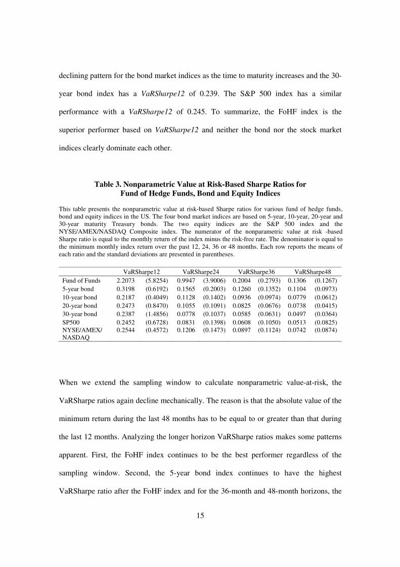
Next, we investigate the reward-to-risk ratios that have parametric value-at-risk based on

Hansen’s (1994) skewed t-density in their denominators. Table 4 presents the results. The

inference from the analysis of PVaRSharpe ratios corroborates the findings from Table 3.

When we focus on the 12-month sampling horizon for the construction of the parametric

downside risk measure, we find that the FoHF index again has the highest reward-to-risk

ratio with a PVaRSharpe12 of 1.104. One can also see that the 10-year bond index also

performs well for this metric with a PVaRSharpe12 of 0.643. The stock market indices,

namely the NYSE/AMEX/NASDAQ and S&P 500 indices have PVaRSharpe ratios of

0.167 and 0.131, respectively. These values are lower than those of all bond market

indices with the exception of the 30-year bond index. The extension of the sampling

window again reduces the reward-to-risk ratios for all indices. The FoHF index continues

17

to be the best performer regardless of the length of the sampling window. However, as

observed for the traditional and nonparametric value-at-risk based Sharpe ratios, the

decline in the PVaRSharpe ratio is steeper than the other indices. For example, the ratio

of PVaRSharpe12 of the FoHF index to that of the 5-year bond index is more than 4

when the 12-month sampling window is used whereas for the 48-month sampling

window, the FoHF and 5-year bond indices have PVaRSharpe ratios of 0.137 and 0.108,

respectively. A closer look at the results reveals that the bond market indices generally

outperform the stock market indices and there is a downward trend in the reward-to-risk

ratios among the bond market indices especially for longer sampling windows.

Table 4. Parametric Value at Risk -Based Sharpe Ratios for

Fund of Hedge Funds, Bond and Equity Indices

This table presents the parametric value at risk-based Sharpe ratios for various fund of hedge funds, bond and equity indices in the US. The four bond market indices are based on 5-year, 10-year, 20-year and 30-year maturity Treasury bonds. The two equity indices are the S&P 500 index and the NYSE/AMEX/NASDAQ Composite index. The numerator of the parametric value at risk-based Sharpe ratio is equal to the monthly return of the index minus the risk-free rate. The denominator is equal to the first percentile of Hansen’s (1994) skewed t-density estimated using the monthly returns from over the past 12, 24, 36 or 48 months. Each row reports the means of each ratio and the standard deviations are presented in parentheses.

PVaRSharpe12 PVaRSharpe24 PVaRSharpe36 PVaRSharpe48

Fund of Funds 1.1037 (4.3839) 0.6146 (1.7954) 0.2264 (0.4187) 0.1365 (0.1729)

5-year bond 0.2456 (0.7375) 0.1326 (0.1711) 0.1168 (0.1265) 0.1082 (0.0956)

10-year bond 0.6431 (7.6812) 0.0971 (0.1222) 0.0877 (0.0916) 0.0782 (0.0597)

20-year bond 0.2614 (1.4548) 0.1058 (0.1848) 0.0840 (0.0739) 0.0761 (0.0422)

30-year bond 0.1306 (0.2904) 0.0924 (0.3949) 0.0606 (0.0755) 0.0525 (0.0409)

SP500 0.1314 (0.2936) 0.0722 (0.1218) 0.0554 (0.0942) 0.0490 (0.0769) NYSE/AMEX/ NASDAQ

0.1666 (0.2965) 0.1035 (0.1253) 0.0833 (0.0993) 0.0726 (0.0799)

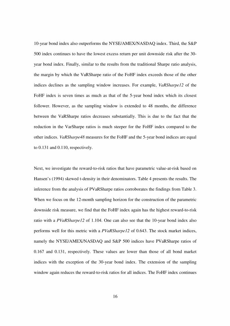
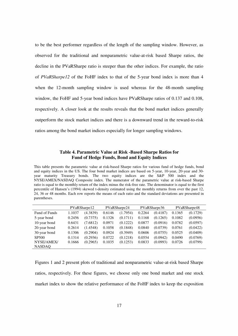
Figures 1 and 2 present plots of traditional and nonparametric value-at-risk based Sharpe

ratios, respectively. For these figures, we choose only one bond market and one stock

market index to show the relative performance of the FoHF index to keep the exposition

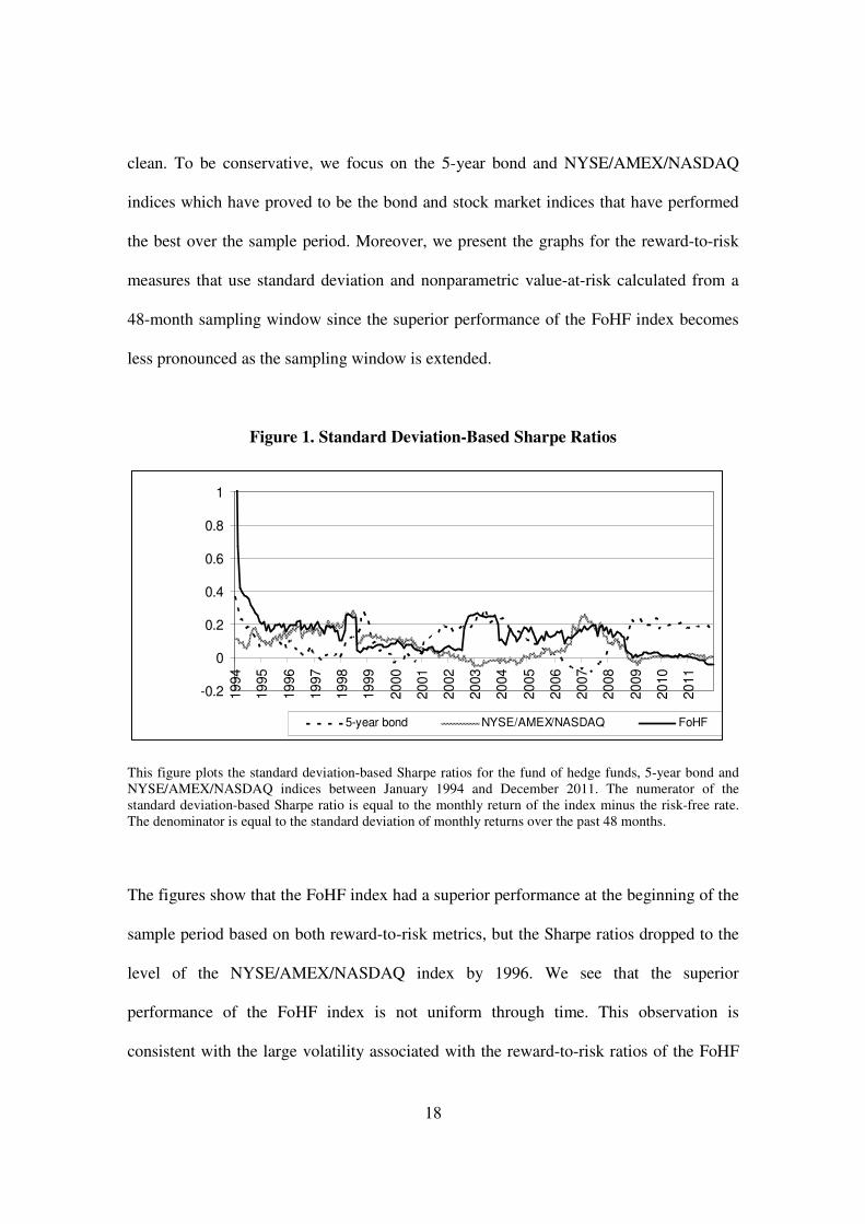
18

clean. To be conservative, we focus on the 5-year bond and NYSE/AMEX/NASDAQ

indices which have proved to be the bond and stock market indices that have performed

the best over the sample period. Moreover, we present the graphs for the reward-to-risk

measures that use standard deviation and nonparametric value-at-risk calculated from a

48-month sampling window since the superior performance of the FoHF index becomes

less pronounced as the sampling window is extended.

Figure 1. Standard Deviation-Based Sharpe Ratios

-0.2

0

0.2

0.4

0.6

0.8

1

19

94

19

95

19

96

19

97

19

98

19

99

20

00

20

01

20

02

20

03

20

04

20

05

20

06

20

07

20

08

20

09

20

10

20

11

5-year bond NYSE/AMEX/NASDAQ FoHF

This figure plots the standard deviation-based Sharpe ratios for the fund of hedge funds, 5-year bond and NYSE/AMEX/NASDAQ indices between January 1994 and December 2011. The numerator of the standard deviation-based Sharpe ratio is equal to the monthly return of the index minus the risk-free rate. The denominator is equal to the standard deviation of monthly returns over the past 48 months.

The figures show that the FoHF index had a superior performance at the beginning of the

sample period based on both reward-to-risk metrics, but the Sharpe ratios dropped to the

level of the NYSE/AMEX/NASDAQ index by 1996. We see that the superior

performance of the FoHF index is not uniform through time. This observation is

consistent with the large volatility associated with the reward-to-risk ratios of the FoHF

19

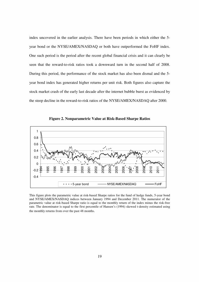
index uncovered in the earlier analysis. There have been periods in which either the 5-

year bond or the NYSE/AMEX/NASDAQ or both have outperformed the FoHF index.

One such period is the period after the recent global financial crisis and it can clearly be

seen that the reward-to-risk ratios took a downward turn in the second half of 2008.

During this period, the performance of the stock market has also been dismal and the 5-

year bond index has generated higher returns per unit risk. Both figures also capture the

stock market crash of the early last decade after the internet bubble burst as evidenced by

the steep decline in the reward-to-risk ratios of the NYSE/AMEX/NASDAQ after 2000.

Figure 2. Nonparametric Value at Risk-Based Sharpe Ratios

-0.4

-0.2

0

0.2

0.4

0.6

0.8

1

1994

1995

1996

1997

1998

1999

2000

2001

2002

2003

2004

2005

2006

2007

2008

2009

2010

2011

5-year bond NYSE/AMEX/NASDAQ FoHF

This figure plots the parametric value at risk-based Sharpe ratios for the fund of hedge funds, 5-year bond and NYSE/AMEX/NASDAQ indices between January 1994 and December 2011. The numerator of the parametric value at risk-based Sharpe ratio is equal to the monthly return of the index minus the risk-free rate. The denominator is equal to the first percentile of Hansen’s (1994) skewed t-density estimated using

the monthly returns from over the past 48 months.

20

CONCLUSION

We investigate whether the fund of hedge fund portfolios outperform various bond and

stock market indices in terms of being able to generate higher returns per unit risk. Due to

the potential non-normality associated with hedge fund returns, we give special emphasis

to the concept of downside risk in our analysis. Consequently, apart from the traditional

Sharpe ratio, we also construct reward-to-risk ratios that use non-parametric or

parametric measures of value-at-risk in their denominator for various indices. Our main

finding is that the FoHF index has superior reward-to-risk ratios compared to all bond

and stock market indices. Although this superior performance is more pronounced when

the risk measures are calculated using data from the last 12 months, the ability of the

FoHF index to generate higher returns per unit risk is robust regardless of the sampling

window. We also find that the documented outperformance is not a phenomenon that has

been observed consistently through time and there have been periods in which the FoHF

index has lagged behind the other indices.

21

REFERENCES

Agarwal, V. and Naik, N.Y. (2004). Risks and Portfolio Decisions Involving Hedge Funds. Review of Financial Studies, 17(1): 63-98. Arditti, F.D. (1967). Risk and the Required Return on Equity. Journal of Finance, 22(1): 19-36. Bali, T.G., Gokcan, S. and Liang, B. (2007). Value at Risk and the Cross Section of Hedge Fund Returns. Journal of Banking and Finance, 31(4): 1135-1166. Brown, S.J., Gregoriou, G. and Pascalau, R. (2012). Is It Possible to Overdiversify? The Case of Funds of Hedge Funds. Review of Asset Pricing Studies, forthcoming. Cornish, E.A. and Fisher, R.A. (1937). Moments and Cumulants in the Specification of Distributions. In: La Revue de l’Institute International de Statistique, 4. Reprinted in Fisher, R.A. (1950). In: Contributions to Mathematical Statistics. Wiley, New York, NY. Dittmar, R.F. (2002). Nonlinear Pricing Kernels, Kurtosis Preference, and Evidence from the Cross Section of Equity Returns. Journal of Finance, 57(1): 369-403. Fung, W. and Hsieh, D.A. (1997). Empirical Characteristics of Dynamic Trading Strategies: The Case of Hedge Funds. Review of Financial Studies, 10(2): 275-302. Fung, W. and Hsieh, D.A. (2000). Performance Characteristics of Hedge Funds and CTA Funds: Natural versus Spurious Biases. Journal of Financial and Quantitative Analysis, 35(3): 291-307. Fung, W. and Hsieh, D.A. (2001). The Risk in Hedge Fund Strategies: Theory and Evidence from Trend Followers. Review of Financial Studies, 14(2): 313-341. Hansen, B.E. (1994). Autoregressive Conditional Density Estimation. International

Economic Review, 35(3): 705-730. Harvey, C.R. and Siddique, A. (2000). Conditional Skewness in Asset Pricing Tests. Journal of Finance, 55(3): 1263-1295. Kimball, M. (1993). Standard Risk Aversion. Econometrica, 61(3): 589-611. Kraus, A. and Litzenberger, R.H. (1976). Skewness Preference and the Valuation of Risk Assets. Journal of Finance, 31(4): 1085-1100. Liang, B. and Park, H. (2007). Risk Measures for Hedge Funds: A Cross-sectional Approach. European Financial Management, 13(2): 333-370.

22

Malkiel, B.G. and Saha, A. (2005). Hedge Funds: Risk and Return. Financial Analysts

Journal, 61(6): 80-88. Markowitz, H. (1952). Portfolio Selection. Journal of Finance, 7(1): 77-91. Mitchell, M. and Pulvino, T. (2001). Characteristics of Risk and Return in Risk Arbitrage. Journal of Finance, 56(6): 2135-2175. Pratt, J. and Zeckhauser, R. (1987). Proper Risk Aversion. Econometrica, 55(1): 143-154. Sharpe, W.F (1966). Mutual Fund Performance. Journal of Business, 39(1): 119-138.