Statistics Netherlands

Discussion paper (201301)

The views expressed in this paper are those of the author(s) and do not necessarily reflect the policies of Statistics Netherlands

The Hague/Heerlen, 2013

213George van Leeuwen and Pierre Mohen

Revisiting the Porter Hypothesis: an emperical analysis of green innovation for the Netherlands

Explanation of symbols

. data not available

* provisional � gure

** revised provisional � gure (but not de� nite)

x publication prohibited (con� dential � gure)

– nil

– (between two � gures) inclusive

0 (0.0) less than half of unit concerned

empty cell not applicable

2012–2013 2012 to 2013 inclusive

2012/2013 average for 2012 up to and including 2013

2012/’13 crop year, � nancial year, school year etc. beginning in 2012 and ending in 2013

2010/’11–2012/’13 crop year, � nancial year, etc. 2010/’11 to 2012/’13 inclusive

Due to rounding, some totals may not correspond with the sum of the separate � gures.

PublisherStatistics NetherlandsHenri Faasdreef 3122492 JP The Hague

Prepress Statistics NetherlandsGrafimedia

CoverTeldesign, Rotterdam

InformationTelephone +31 88 570 70 70Telefax +31 70 337 59 94Via contact form: www.cbs.nl/information

Where to orderE-mail: verkoop@cbs.nlTelefax +31 45 570 62 68

Internetwww.cbs.nl

ISSN: 1572-0314

© Statistics Netherlands, The Hague/Heerlen, 2013.Reproduction is permitted, provided Statistics Netherlands is quoted as source.

60083201301 X-10

3

REVISITING THE PORTER HYPOTHESIS: AN EMPIRICAL ANALYSIS OF GREEN INNOVATION FOR THE NETHERLANDS

George van Leeuwen1 and Pierre Mohnen2

Abstract

Almost all empirical research that has attempted to assess the validity of the Porter Hy-pothesis has started from reduced-form models, e.g. by using single-equation models for estimating the contribution of environmental regulation (ER) to productivity. This paper addresses the Porter Hypothesis within a structural approach that allows us to test what is known in the literature as the “weak” and the “strong” version of the Porter hypothesis. Our “Green Innovation” model includes three types of eco investments and non-eco R&D to explain differences in the incidence of innovation. Besides product and process innovations we recognize eco-innovation as a separate type of innovation output. We explicitly model the potential synergies of introducing the three types of innovations simultaneously and their synergy in affecting total factor productivity (TFP) performance. Using a comprehensive panel of firm-level data built from four surveys we aim to estimate the relative importance of energy price incentives as a market based type of ER and the direct effect of environmental regulation on eco investment and firms’ decisions regarding the introduction of several types of innovations. The results of our analysis show a strong corroboration of the weak version of the Porter hypothesis but not of the strong version of the PH, in this case on TFP per-formance.

Keywords: Porter Hypothesis, green innovation, environmental regulation, innovation com-plementarities, productivity.

JEL codes: H23, L5, O32, O38, Q55

The first author expresses his gratitude for being able to carry out this research as a visiting fellow at UNU-MERIT. The views expressed in this paper are those of the authors and do not necessarily reflect any policy by Statistics Netherlands. We thank Jacques Mairesse and Georg Licht for helpful comments. 1 Statistics Netherlands. 2 UNU-MERIT and Maastricht University.

4

1. Introduction

The relationship between technological change and environmental policy has received a lot of attention from scholars and policymakers during the last decades. This is partly because the environmental consequences of social and business activ-ity are affected by the rate and direction of technological change, and also because environmental policy interventions may create new constraints and incentives that may shape the path of future technological development (Jaffe et al., 2003).

Environmental technological progress is a very broad phenomenon and every description of it cannot be more than very incomplete. Some examples concern 1) technologies that reduce pollution at the end-of-pipe, such as scrubbers for use on industrial smokestacks or catalytic converters for automobiles 2) technologies that increase user value for consumer products (e.g. medicines) after introducing new production methods, which, at the same time, decrease the environmental burden of their production by using materials that are less harmful for the environment and 3) implementation of technologies that are targeted to changes in production processes to improve energy efficiency.

Policy responses to environmental problems often start from the assertion that the link between overall technological change and (e.g.) climate based environ-mental policies is merely macro oriented. However, for understanding the interac-tion between environmental policy and technology it also makes sense to go down to the micro level. After all, environmental regulation and public funding of R&D are the first impetus to have more green technologies developed by individual firms. Similar to other types of innovations, the benefits of environmental technological innovations may accrue to society at large rather than to the adopter of these new technologies alone. This market failure related to innovation in general is pivotal to the numerous discussions surrounding the so-called Porter-Hypothesis (PH).

It is often argued (see e.g. Wagner, 2003) that one cannot find a 10-Dollar bill on the ground, because if it was there, somebody else would already have picked it up. This metaphor neglects three things 1) that market forces alone do not provide enough incentives for firms to be engaged in green innovation and 2) that green innovation is not very different compared to innovation in general and 3) that policy responses such as environmental regulation have a role to play to bring economic opportunity in line with the environment (see e.g. Jaffe et al., 2002, Desrochers, 2008 and Cerin, 2012). The central issue is the question whether regulation drives innovation. The PH asserts that polluting firms can benefit from environmental poli-cies, arguing that well designed and stringent environmental regulation (ER) can stimulate innovations, which in turn increase the productivity of firms or the product value for end users (Porter, 1991; Porter and van der Linde, 1995). The message of this hypothesis is that there seems to be no trade-off between economic growth and environmental protection but a win-win situation instead. Environmental regulation would benefit both society and regulated firms by triggering dynamic efficiency of firms and these benefits may partially or fully offset the costs of complying with environmental restrictions.

5

The empirical evidence available supporting the Porter Hypothesis seems to be rather scanty and in most cases the PH is rejected by the data (see e.g. Wagner (2003), Popp et al. (2010), Ambec and Barla (2006), and Ambec et al. (2011) for an extended review). For the Netherlands the evidence seems to be very scarce. This paper tries to shed a new light on the PH by using a rich unbalanced panel con-structed by matching Dutch firm level data from four surveys and by modeling the complementarities of eco-innovation with traditional modes of innovation.

As argued by Kriegel and Ziesemer (2009), the main problem regarding the empirical testing of the PH, in essence, boils down to having a better understanding of the (eco) innovation adoption decisions of firms. This assertion asks for a struc-tural modeling approach in investing the contribution of energy prices and environ-mental regulations on green investment and of green investment on innovation and productive efficiency. We will embark on this task by adopting a Green CDM (Cré-pon-Duguet-Mairesse) type of model for the Netherlands, similar to the Lanoie, Laurent-Lucchetti, Johnstone and Ambec (2011) model, that allows testing what Jaffe and Palmer (1997) have called the “weak” version and the “strong” version of the PH, referring to the effect of environmental regulations on respectively environ-mental innovations and economic performance, in this case total factor productivity (TFP). Contrary to Cainelli et al. (2010) our model includes several types of eco investments and regards eco innovation as a special mode of innovation output. Eco, environmental and green innovation will be interchangeably used, indicating each time an innovation with a lower environmental impact. Likewise eco, environmental and green investment all point to investments aimed at reducing the environmental burden of production (for more discussion on the definition, see Kemp (2011)).

Our starting point of investigation of the PH is the impact of energy prices on different types of eco investment. The fact that carbon taxes are a substantial part of gross energy prices makes them a potentially useful instrument for environmental policy aimed at improving the energy related static as well as dynamic efficiency of firms. In particular, this may be the case if such price incentives invoke environ-mental investment combined with the renewing of the production process (so-called process integrated eco investment).

Our empirical model starts from the estimation of four innovation input equa-tions: two for R&D (eco R&D and other R&D) and two for other types of eco-investments, end-of-pipe and process integrated respectively. Subsequently, we use the predictions from these equations for modeling the incidence of different types of innovation. At the end, we will estimate a labor productivity equation and test for complementarity or substitutability of different innovation strategies in affecting the total factor productivity (TFP).

A novelty of our paper is that we try to assess the existence of complementari-ties (as defined in Milgrom and Roberts, 1990 and 1995) between product, process and eco innovations. We distinguish complementarities in the incidence of innova-tion and in their effects on productivity performance. To estimate the structural model we have implemented a procedure proposed by Lewbel (2007) for solving the

6

coherency and incompleteness problem when estimating a system of equations with dummy endogenous variables.

The plan of the paper is as follows. In section 2 an overview of the literature is given. Section 3 discusses the model used in the empirical application and elabo-rates on the econometric issues of this research. Thereafter the data are presented in section 4, followed by a discussion of the main results in section 5. Section 6 con-cludes.

2. Literature review

One can hardly find any branch of economics that has been concerned with the PH as much as environmental economics. There is a vast body of literature de-voted to appraise or peruse the seminal contributions of Porter (1991) and Porter and van der Linde (1995). Originating primarily from empirical regularities found in the analysis of cross-country differences in the stringency of environmental regulation and economic performance, the hypothesis has triggered a lot of research both theo-retical and empirical in nature. The Porter hypothesis has been criticized, for being merely based on anecdotal stories (which in some cases seem to be even erroneous) and for the lack of a sound theoretical basis (see e.g. Palmer et al., 1995, and Cerin, 2006).

More recent research attempts to fill the gap between empirics and theory to provide a theoretical underpinning of the PH. Mohr (2002) argues that it is a feasible outcome if one allows for the possibility of endogenous technical change. More recent theoretical contributions that link the environment to endogenous growth are given in Acemoglu et al. (2012) and Gans (2012). Ambec and Barla (2002) raise the question whether regulation is indeed needed for firms to adopt profit-increasing innovations, and pointing amongst others to the 10-Dollar metaphor mentioned above. This last criticism is targeted to the primitive of the PH stating that firms systematically ignore opportunities for profit increasing innovations and that envi-ronmental regulation can motivate firms to capture “low hanging fruit” offered by environmental challenges to their businesses. Another source is the literature of be-havior economics. This literature offers several explanations for underinvesting in environmental innovation (see e.g. Ambec and Barla, 2006, for examples).

Similarly, several theoretical attempts have tried to frame regulation in mod-els often used for analyzing the interaction between competition and innovation. A recent example is given in Constantatos and Hermann (2011). The example concerns the introduction of organic products in Pharmaceutical Manufacturing. By avoiding the use of environmentally damaging fertilizers there is less environmental burden as well as more user value created because organic drugs are healthier. In this case a win-win situation between regulation and innovation is not self-evident because there is much scope for conjectural variation, especially if such innovations take place in markets that are characterized by fierce competition and because the envi-

7

ronmental quality of the new product will be highly correlated with other product attributes. The latter argument explains why inertia at the consumer side of the mar-ket may enlarge the risk of investing due to potential first-mover disadvantages.

The example illustrates that there are many similarities with the traditional view on the relationship between innovation and competition as a source of underin-vesting in innovation. Moreover, the example also shows that the scope for envi-ronmental policies is very broad in principle, but that it is questionable how envi-ronmental regulation can offer a solution to the problems involved. This brings us to another strand of research that focuses on the second primitive of the PH, i.e. the assertion that environmental regulations should be well designed and stringent enough to be successful also from an economic point of view.

An assessment of the instruments of environmental regulation and a judgment of their effectiveness can be found in Wagner (2003). The myriad of environmental instruments can be better understood when using a classification or typology. A first delineation is between command and control type regulation and market based regu-lation. The instruments that set emission limits and standards fall into the first class and are often labeled “end of pipe” regulations. Environmental taxes and charges and tradable emission permits or certificates are examples of the second class of instruments.

Environmental effectiveness can be defined as the ability to achieve a prede-fined environmental target. The general view is that this definition is more appropri-ate for the first class of instruments. By contrast, the second class of instruments has a higher economic profile, because they are aimed at triggering static and dynamic efficiency and internalizing environmental externalities in and between markets. In particular these instruments play a role in the empirical testing of the premises of the PH.

Looking at the empirical evidence provided in the literature it can be con-cluded that the picture is rather mixed. The number of papers and articles that have put the PH to the empirical testing is overwhelming but they do not to lead to a gen-eral consensus. Much of this has to do with the different research strategies and the availability of data. Compared to empirical evidence at the macro or industry level, the number of papers that use firm level data is rather scarce. Besides that, research is targeted at different measures of performance.

Cutting through different reviews of empirical work it can be concluded that much research is aimed at investigating the impact of environmental regulation on productivity or productive efficiency in a reduced form estimation approach. In many cases this type of research leads to the conclusion that environmental regula-tion has a negative impact on productivity. This conclusion can be easily under-stood, because regulation forces firms to invest in the environment and this increases production costs of firms to comply with the environmental restrictions.

There are several issues at stake here. If these investments do not lead to re-newing of production processes then there is no reason for expecting substantial

8

gains in resource efficiency. A second issue is related to measurement. “End-of-pipe” investments may reduce pollution but this reduction is not accounted for in output. The same capital and other inputs produce two types of output: bad and good output and it is hardly possible to value the contribution of (reducing) bad output. This raises serious problems when investigating the relation between environmental regulation and (productive) efficiency.1 An interesting solution to circumvent this problem is presented in Domazlicky and Weber (2004). They use volume data on toxic releases and traditional output measures such as real value added in a non-parametric analysis to identify technical change from efficiency change. However, these results also lead to the conclusion that the impact of regulation on total factor productivity (TFP) is negative.2

More interesting for the PH is the research that looks into the impact of envi-ronmental regulation on innovation. This type of research seems to be a necessary if not sufficient condition for the PH. Again the evidence is scanty and weak in gen-eral. Notable examples of this type of research can be found in several papers and articles of ZEW. In most cases the research uses the data collected on innovation and regulation in the Mannheim Innovation Panel that is constructed from several editions of the German Community Innovation Survey (CIS). The focus of research varies between regulation driven innovation alone (Rennings and Rexhäuser, 2010) to the impact of regulation driven innovation on competitiveness (Rennings and Rammer, 2010), employment dynamics (Horbach and Rennings, 2012) or profitabil-ity (Rexhäuser and Rammer, 2011). Support for the PH is provided by concluding that environmental regulation does not harm competitiveness (Rennings and Ram-mer, 2010) and that the contribution of regulation induced innovation to profitability is larger than the contribution of other (more) voluntary innovations (Rexhäuser and Rammer, 2011).

Ideally, a thorough empirical testing of the PH requires data on which types of regulations trigger which innovations at the firm level. The most recent edition of CIS contains new questions on environmental innovation. However, for the Nether-lands, this new module cannot be used to identify the role of different instruments of environmental regulation properly. The only variable available on regulation in this research concerns firm responses to environmental regulation in general, either ex-isting or anticipated regulations. By contrast, the German CIS allows a distinction between types of environmental regulations. After matching the firm responses with external data on the age of regulations, Rennings and Rexhäuser (2010) also investi-gated the long-term impact of different types of regulation on the adoption of envi-ronmental innovation. To keep things tractable, they made a distinction between three types of environmental regulation (ER): a) “end-of-pipe” regulation, b) circu-lar flow economy regulation and c) climate change based regulations. An important conclusion is that the long-term impact of regulation only triggers innovation that is

1 This problem is well recognized by statisticians and environmental accounting is an important avenue for National Accounts. See Muller et al. (2011) for a recent contribution to this problem. 2 The method used is the “directional output distance approach” developed by Chung et al. (2007) for constructing the Malmquist-Luneberger index to decompose (changes in) TFP.

9

strongly related to “control type” ER. By contrast, the support for PH in terms of increasing static or dynamic efficiency is limited. As convincingly argued by Ren-nings and Rexhäuser (2010), the contribution of control type ER to dynamic effi-ciency is expected to be limited, as, once installed, “end-of pipe” environmental investment cannot contribute to the innovation process anymore.

One can add to this that other types of ecological investment may yield higher returns to investment. Combining eco investment with renewing of production proc-esses seems a better example of innovation related eco investment. We take this consideration into account in the next section.

Energy price incentives (taxes)

Innovation expenditure (R&D), Environmental investment

Environmental Regulation

Knowledge capitalDemand pull

technology push

Innovations, patents

PH

Productivity/Resource efficiency

Capital, labor

“Green CDM model (Crépon-Duguet-Mairesse, 1998)”

3. A Green CDM type empirical model

The empirical model used in this paper is a modified version of the so-called “CDM model”. Today, this model is the work horse for research on innovation when using firm-level data (see Crépon, Duguet and Mairesse, 1998). A graphical presen-tation of our model is given in Figure 1.3 The upper part of the figure points to the investment decision stage. In the traditional CDM model this concerns the decision on how much to invest in R&D. In this paper we face another investment decision problem, i.e. namely whether or not to invest in order to reduce the environmental burden of the firm’s operations. In section 3.1 we will discuss the specification of the input stage of the model. The second block of the model describes innovation a separate production process with R&D and eco-investment as an input and knowl-

3 The figure is adapted version of the one presented in Crépon, Duguet and Mairesse (1998).

10

edge creation, in the form of new products, new production processes and eco-innovation as the outcomes.

The third block examines the link between innovation outputs and productiv-ity as a measure of economic performance. We shall now describe each block in detail.

3.1 The investment decisions

We consider four investment decisions: three decisions concerning types of

eco investment and one concerning investment in non-eco R&D. Eco investment (X1) is comprised of 1) eco R&D, 2) eco investment in end-of-pipe facilities, and 3) eco investment that is “process integrated”, i.e. eco investment combined with the renewal of the main production processes of the firm. The investment inputs into non-eco innovation (X2) are defined as gross expenditures in R&D less expenditures in eco R&D. Irrespective of which type of investment is concerned, we assume that firms first decide whether to invest or not and then choose the investment intensity.

Firms will invest in each of these types of investment if the latent value of in-vesting exceeds some threshold value c . For example, for X1, this can be expressed as follows:

11 =iDX if 1111

*1 cZDX iii >+′= εα , and

(1) 01 =iDX if 1111

*1 cZDX iii ≤+′= εα .

The vector Zi1 in (1) collects the variables that are assumed to determine the selec-tion of firms that invest in X1, i.e. the occurrence of having performed and reported eco investment of the type considered. In a similar way we can model the decision concerning non-eco R&D investment (DXi2).

Model (1) is extended with a set of equations that models the level of invest-ment intensity for each of the three types of eco investment and for non-eco R&D. For example, for some type of eco investment, this yields

111*11 iiii eXXX +′== β if 11 =iDX , and

(2)

01 =iX if .01 =iDX

Models (1) and (2) are applied to each of the four types of innovation invest-

ment. Assuming a bivariate normal distribution for 1ε and 1e (in case of a specific

type of eco investment), and similarly for 2ε and 2e (in case of non-eco R&D in-

vestment), the system (1) - (2) is a Tobit II type selection model (Amemiya,1984).

11

3.2 Implementing the investment models

Although we are dealing in each case with a general investment problem, one can imagine that the four types of investment are rather distinct. The traditional view is that expenditures on non-eco R&D have a higher economic profile, and that such expenditures are quite different from eco investment (including eco R&D) when judged from the point of the strategies of the firms. This is in particular the case if we compare eco investment performed to comply with “control type” environmental regulation with R&D that is aimed at developing new goods.

Not at least because of the difficulty of evaluating the output of “bad goods” or of “process integrated” eco investment, which, by definition aims at reducing bad output and increasing resource efficiency, it is impossible to use standard capital and investment theory to derive formal investment models. At least, we consider such an exercise beyond the scope of this research. To a lesser extent the same prob-lems also carries over to “process integrated” eco investment, which, by definition aims at reducing bad output while increasing resource efficiency. Likewise for in-vestment in non-eco R&D, we miss the necessary price data to estimate an invest-ment equation that would be embedded in capital and investment theory. For both eco-and non-eco investments we have information on subsidies received that can be used for explaining differences in investment intensities between firms. The R&D subsidies are not the only incentives for eco R&D (and investment). Internalizing environmental externalities can also be achieved via energy prices. As mentioned before, energy prices are an interesting instrument of market based ER. A nice fea-ture of the data is that we can construct firm-specific marginal energy prices to ex-plain differences in each type of eco investment. This brings us to the specification of the vectors Z and X in (1) and (2) for non-eco R&D innovation investment and for the three types of eco investment respectively.

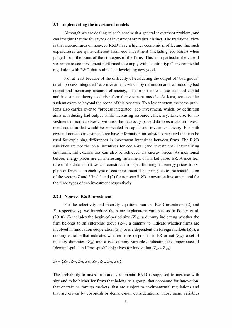
3.2.1 Non-eco R&D investment

For the selectivity and intensity equations non-eco R&D investment (Z2 and X2 respectively), we introduce the same explanatory variables as in Polder et al. (2010). Z2 includes the begin-of-period size (Z21), a dummy indicating whether the firm belongs to an enterprise group (Z22), a dummy to indicate whether firms are involved in innovation cooperation (Z23) or are dependent on foreign markets (Z24), a dummy variable that indicates whether firms responded to ER or not (Z25), a set of industry dummies (Z26) and a two dummy variables indicating the importance of “demand-pull” and “cost-push” objectives for innovation (Z27 - Z 28):

Z2 = {Z21, Z22, Z23, Z24, Z25, Z26, Z27, Z28}.

The probability to invest in non-environmental R&D is supposed to increase with size and to be higher for firms that belong to a group, that cooperate for innovation, that operate on foreign markets, that are subject to environmental regulations and that are driven by cost-push or demand-pull considerations. Those same variables

12

are assumed to affect the intensity of non-eco R&D, i.e. are collected in the vector X2, with the exception of the innovation cooperation dummy (Z23) and with the addi-tion of subsidies received from local authorities, government bodies and the EU (X21 - X23) and a set of time dummies (X24). Hence we have

X2 = {Z21, Z22, Z24, Z25, Z26, X21, X22, X23, X24}.

3.2.2 Eco investment

In principle, some of the variables used for modeling other innovation invest-ment could also be used for the eco investment equations (Z1 and X1). However, this would lead to a considerable loss of data at the outset because of the small overlap of the data of the four surveys that would have to be matched (see section 5). To minimize the lack of data coverage between surveys, we focus on the variables that are collected in two surveys: the Production Statistics survey (PS) and the survey on environmental costs of firms (ECF). The use of ECF is imperative here. It is this survey that collects data on the three types of eco investment. Combining these with data on energy costs and volumes collected in the PS-survey allows us to construct (gross) marginal energy prices (pegt) for the firms for which data on eco investment are available.4 In this way, and after using a measure for the prices of eco investment collected in the ECF survey (pit), we obtain a measure for the relative price of eco investment (relative to energy prices)

).ln()ln(11 gtt pepiX −=

Furthermore, and to determine the importance of ER for eco investment, we include an environmental regulation (ER) dummy (X12). The model is “completed” further by using the logarithm of beginning-of-period energy cost shares (X13), the logarithm of beginning-of-period size (X14), a dummy variable that indicates whether firms received eco subsidies (X15), and a set of industry and year dummies (X16):

X1 = {X11, … , X16}.

Finally, we take into account that selectivity may be dependent on the responses to ER (X12), on the (pre-existing) energy intensity (X13), on firm size (X14), on the im-portance of (pre-existing) environmental levies (X17) and on a set of industry dum-mies (X18):

4 For a much smaller sample (obtained after matching also the “Energy Use Survey” (ES)) we can decompose gross marginal energy prices as follows:

),1( ntntntntgt stepetepepe +=+=

where pent is the marginal energy price net of taxes, tent the marginal energy tax and stent the ratio of marginal energy tax over marginal energy prices net of taxes. Constructing this variable is only possi-ble for the intersection of ES and PS data. Matching this intersection with the CIS and ECF data leads to a considerable loss of data.

13

Z1 = { X12, X13, X14, X17, X18}.

3.3 Innovation output

The middle part of figure 1 indicates that innovation investment leads to in-novation output. We consider three types of innovation output: product -, process - and eco innovation. We observe dichotomous variables indicating whether a certain innovation has been adopted or not. The three types of innovation are likely to be interrelated in the sense that the return to a certain type of innovation could depend on the adoption of the other innovations for reasons of complementarity or substitut-ability between them. It is well documented in the econometric literature (see e.g. Heckman, 1978, Tamer, 2003, Lewbel, 2007) that the estimation of a trivariate pro-bit with endogenous dummy variables raises severe problems of identification. There can be no solution (in which case the system is said to be incoherent) or mul-tiple solutions (in which case it is said to be incomplete). The empirical literature offers several solutions to this problem. In general, these solutions boil down to im-posing zero restrictions on the coefficients of some of the binary endogenous ex-planatory variables or by relying on recursive or triangular systems in which one of the choices is assumed to be leading (see for a discussion of completeness and co-herency section 2 of Tamer (2003)). One way to avoid incoherency and incomplete-ness is to start from a McFadden (1973) solution by considering a multinomial choice problem based on a random utility model. This framework has been proposed more recently by Lewbel (2007) and adapted by Miravete and Pernías (2006) and Kretschmer, Miravete and Pernías (2012).

Let the total utility (in this case profit) be

== ),,( 321 yyyVV

++++′ 1131321211 )( yyyx εααβ (3)

++++′ 2232312122 )( yyyx εααβ

.)( 3323213133 yyyx εααβ +++′

The dichotomous variables for the three types of innovation are given by ).3,2,1( =iyi There are in total eight possible combinations of innovation choices

yielding respectively the following profit outcomes:

0)0,0,0( =V (3a)

333)1,0,0( εβ +′= xV (3b)

222)0,1,0( εβ +′= xV (3c)

3232233322 )()1,1,0( εεααββ ++++′+′= xxV (3d)

111)0,0,1( εβ +′= xV (3e)

14

3131133311 )()1,0,1( εεααββ ++++′+′= xxV (3f)

2121122211 )()0,1,1( εεααββ ++++′+′= xxV (3g)

332211)1,1,1( xxxV βββ ′+′+′=

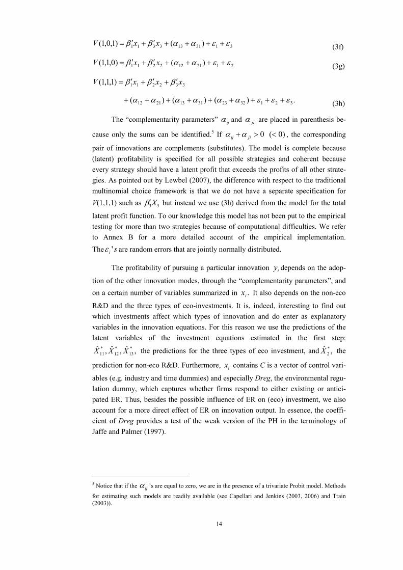
.)()()( 321322331132112 εεεαααααα +++++++++ (3h)

The “complementarity parameters” ijα and jiα are placed in parenthesis be-

cause only the sums can be identified.5 If 0>+ jiij αα )0(< , the corresponding

pair of innovations are complements (substitutes). The model is complete because (latent) profitability is specified for all possible strategies and coherent because every strategy should have a latent profit that exceeds the profits of all other strate-gies. As pointed out by Lewbel (2007), the difference with respect to the traditional multinomial choice framework is that we do not have a separate specification for V(1,1,1) such as 33Xβ′ but instead we use (3h) derived from the model for the total

latent profit function. To our knowledge this model has not been put to the empirical testing for more than two strategies because of computational difficulties. We refer to Annex B for a more detailed account of the empirical implementation. The si 'ε are random errors that are jointly normally distributed.

The profitability of pursuing a particular innovation iy depends on the adop-

tion of the other innovation modes, through the “complementarity parameters”, and on a certain number of variables summarized in .ix It also depends on the non-eco

R&D and the three types of eco-investments. It is, indeed, interesting to find out which investments affect which types of innovation and do enter as explanatory variables in the innovation equations. For this reason we use the predictions of the latent variables of the investment equations estimated in the first step:

,ˆ,ˆ,ˆ *13

*12

*11 XXX the predictions for the three types of eco investment, and ,ˆ *

2X the

prediction for non-eco R&D. Furthermore, ix contains C is a vector of control vari-

ables (e.g. industry and time dummies) and especially Dreg, the environmental regu-lation dummy, which captures whether firms respond to either existing or antici-pated ER. Thus, besides the possible influence of ER on (eco) investment, we also account for a more direct effect of ER on innovation output. In essence, the coeffi-cient of Dreg provides a test of the weak version of the PH in the terminology of Jaffe and Palmer (1997).

5 Notice that if the ijα ’s are equal to zero, we are in the presence of a trivariate Probit model. Methods

for estimating such models are readily available (see Capellari and Jenkins (2003, 2006) and Train (2003)).

15

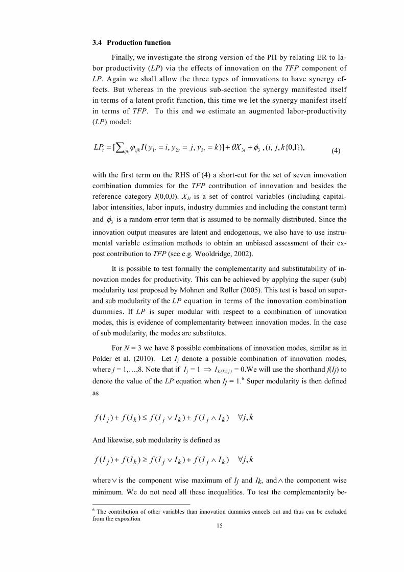
3.4 Production function

Finally, we investigate the strong version of the PH by relating ER to la-bor productivity (LP) via the effects of innovation on the TFP component of LP. Again we shall allow the three types of innovations to have synergy ef-fects. But whereas in the previous sub-section the synergy manifested itself in terms of a latent profit function, this time we let the synergy manifest itself in terms of TFP. To this end we estimate an augmented labor-productivity (LP) model:

33321 )],,([ φθϕ ++==== ∑ tttijk tijkt XkyjyiyILP }),1,0{,,(, kji (4)

with the first term on the RHS of (4) a short-cut for the set of seven innovation combination dummies for the TFP contribution of innovation and besides the reference category I(0,0,0). X3t is a set of control variables (including capital-labor intensities, labor inputs, industry dummies and including the constant term) and 3φ is a random error term that is assumed to be normally distributed. Since the

innovation output measures are latent and endogenous, we also have to use instru-mental variable estimation methods to obtain an unbiased assessment of their ex-post contribution to TFP (see e.g. Wooldridge, 2002).

It is possible to test formally the complementarity and substitutability of in-novation modes for productivity. This can be achieved by applying the super (sub) modularity test proposed by Mohnen and Röller (2005). This test is based on super- and sub modularity of the LP equation in terms of the innovation combination dummies. If LP is super modular with respect to a combination of innovation modes, this is evidence of complementarity between innovation modes. In the case of sub modularity, the modes are substitutes.

For N = 3 we have 8 possible combinations of innovation modes, similar as in Polder et al. (2010). Let Ij denote a possible combination of innovation modes, where j = 1,…,8. Note that if I j = 1 ⇒ Ik (k# j ) = 0.We will use the shorthand f(Ij) to denote the value of the LP equation when Ij = 1.6 Super modularity is then defined as

)()()()( kjkjkj IIfIIfIfIf ∧+∨≤+ kj,∀

And likewise, sub modularity is defined as

)()()()( kjkjkj IIfIIfIfIf ∧+∨≥+ kj,∀

where∨ is the component wise maximum of Ij and Ik, and∧ the component wise minimum. We do not need all these inequalities. To test the complementarity be- 6 The contribution of other variables than innovation dummies cancels out and thus can be excluded from the exposition

16

tween two innovation modes, we only need to make pairwise comparisons keeping the third mode constant. In addition, some inequalities are trivial. For example, for Ij= (0,0,0) and Ik = (1,1,0) we have

f(0,0,0) + f(1,1,0) < f(1,1,0) + f(0,0,0).

Only the combinations where the minimum and maximum operators lead to different combinations than the left-hand sides are non-trivial. Thus, combination Ijshould have at least one element that is smaller than the corresponding element in Ik,and at least one element should be bigger (i.e. at least one innovation mode should occur in Ij but not in Ik and vice versa). For testing the complementarity between, for example, product (y1) and process innovation (y2) in the three-dimensional case, we therefore have Ij = (0,1,D) and Ik = (1,0,D), with D = {0,1}, and the ine-quality restrictions are:

,0)0,0,0()0,1,1()0,0,1()0,1,0( 000110100010 ≤−−+⇔+≤+ ϕϕϕϕffff

.0)1,0,0()1,1,1()1,0,1()1,1,0( 001111101011 ≤−−+⇔+≤+ ϕϕϕϕffff

Similar inequality conditions can be derived for the (conditional) pairwise comparisons of the TFP regression coefficients pertaining to other innovation combinations. Furthermore, the inequalities for sub modularity are easily obtained by replacing ‘<=’ with ‘>=’. Kodde and Palm (1986) derived a Wald test-statistic for testing these inequalities for regression coefficients.

For N = 3 },,,,,,,{ 111110101100011010001000 ϕϕϕϕϕϕϕϕϕ = is the vec-

tor of coefficients on the dummies for innovation mode combinations in the aug-mented T F P mo d e l . We will apply the Kodde-Palm (Kodde and Palm, 1986) test using the IV estimates )( IVϕ of (4).

4. Data

We have constructed a comprehensive dataset by linking firm-level data (manufacturing only) for 2000 – 2008. These data were sourced from four surveys:

1) The survey on environmental costs of firms (ECF). The survey covers the years 2000 – 2008 and beyond. This is one of the most important data sources in this re-search project. The survey collects (amongst others) data on environmental current exploitation costs, two types of environmental investment, environmental subsidies and expenses on environmental R&D. Environmental investment other than eco R&D can be broken down into “end-of-pipe” investment and investment related to the renewing of production processes (so-called “process integrated eco invest-ment”). Because of the fact that this survey only collects data for manufacturing, our empirical analysis will be restricted to this branch of the economy.

17

2) The energy use survey (ES), which covers the same period as the ECF Survey. This survey collects volume data on energy consumption of different types of energy use and these can be used to construct marginal energy prices at the firm-level after linking with the data on energy costs collected in the Production Surveys. As natural gas and electricity are the most important energy sources for almost all firms, our measures for energy prices will be derived from firm-level data for these two energy sources. The data for the two types of energy can be lumped into one measure by using weights that reflect the energy content in TJ of each constituent source of en-ergy. Another interesting contribution of this data source is that it enables the calcu-lation of the carbon-tax component of (gross) marginal energy prices for gas and electricity by using data on the energy price tariff structures (tariff schemes) and the tax structure of energy prices for these two types of energy use. For a limited num-ber of firms we can thus make a distinction between gross marginal energy tariffs and the carbon tax component of gross marginal energy tariffs for the two types of energy. But this exercise is only possible for the firms sampled in the ES-survey. Because of the poor coverage of ES with CIS we face a considerable loss of data when trying to account for the carbon-tax component of energy prices as well as for ER. We have estimated some eco-investment equations with carbon taxes included, but the core models presented in this paper are based on marginal energy prices without paying attention to carbon taxes.

3) The Community Innovation Surveys for 2002-2004, 2004-2006 and 2006-2008. This survey is used to obtain data on the various types of innovation adopted, the R&D inputs into (technological) innovation and other variables, such as e.g. the dependence on foreign markets, innovation subsidies received from different bodies and innovation cooperation. The final edition of CIS can be used to investigate the synergies of simultaneously adopting environmental innovations targeted at produc-tion cost reductions and environmental innovations targeted at decreasing the envi-ronmental burden of final consumption by creating new user value. Because all firms responded to the question on environmental regulation (existing or anticipated) this variable can be seen as an important determinant for explaining synergy effects among innovations.

4) The Production Statistics Survey (PS). This survey contains firm-level data on gross output, turnover, value added, intermediate inputs and the total energy costs of firms. After matching with industry-level deflators, this source can be used to con-struct different output measures such as value-added and gross-output productivity, energy cost shares and profitability.

Table 1a summarizes the coverage of different surveys for manufacturing be-fore and after data linking and before deleting “item non-response” and/or implausi-ble values (such as a recorded negative value added). The ECF survey has the high-est coverage with PS. The ES survey can be considered as the best source for vol-ume data on energy use and the distinction between marginal energy prices net of carbon-taxes and the carbon-tax component of gross marginal energy prices. But its match with ECF and PS (which collects data on energy costs and volumes for gas

18

and electricity) is rather poor.7 A similar poor match can also be found when linking ES to CIS (not shown in the table).

For this reason we choose not to start with the data that are available after matching all four available surveys. Instead we use two separate blocks of data: for the model-ing of the three types of eco investment (including eco R&D) we use the ECF&PS panel and after calculating (gross) marginal energy prices using the data available on the volumes of energy use for gas and electricity in the PS survey and the corre-sponding energy price tariff schemes published by SN. For non-eco R&D innovation investment we use the ECF&CIS-panel for distinguishing between eco R&D and non-eco R&D.8 Thereafter, the predictions from the innovation investment models are used for modeling the decisions to innovate. At this stage the CIS data are im-perative, not at least as this is the only source that collects data on the importance of ER (either existing or anticipated). Annex A presents a list of the variables that are available for assessing the PH in this study. A subset of these variables is used in the empirical application.

Table 1b summarizes some descriptive statistics for the variables used in the models. We restrict the discussion to some interesting results. It is noticeable that when the CIS data are merged with the PS and ECF data some variables, such as firm size, eco-R&D per employee, eco-investment and eco subsidies received, dis-play a higher average than before the merging. This is due to the fact that the CIS survey uses relatively larger firms.9 The means of the variables that originate from the CIS survey do not change very much after merging with other surveys. It can be seen that eco-R&D is considerably lower than other (non-eco) R&D investment. The share of eco-R&D in total R&D investment expenditure amounts to 30 %. Further-more, the share of process integrated eco investment in total eco investment (eco R&D excluded) is about 44 %. These percentages remain of the same order of mag-nitude when calculated for the full panel obtained after linking the PS, ECF and CIS surveys. Finally, it can be seen that about 31 % of the firms in this panel responded to ER, either existing or anticipated.

7 These surveys are carried out every year. 8As CIS collects data on total R&D, only this match enables a distinction between eco - and non-eco R&D. 9The main objective of the ES survey is to produce aggregate energy statistics and the distribution of energy use is very skewed to the right.

Table 1a: Sample coverage (manufacturing only)

PS CIS ECF ES ECF&PS ES&ECFECF&PS

&CIS

2002 5751 8782 1647 4246 12072004 4966 2538 7867 1851 3732 1294 14412006 4300 2133 7296 1683 3344 1110 12382008 3808 2164 7230 1602 3156 989 1289

19

A more detailed account of the distribution of some key variables is given in table 1c. In general the distributions are very skew, with small values for the bulk of firms and relatively few firms with substantial eco R&D or other types of eco in-vestment. However, it can also be seen that eco investment is relatively more “proc-ess integrated” if eco-investment is more substantial. Finally, skewness is relatively much smaller for the productivity measures used in this study.

20

Table 1b: Descriptive statisticsPS&ECF * CIS ** PS&ECF&CIS **N Mean std N mean std N mean std

eco R&D per fte (1000 Euro) 19090 0.094 0.249 3784 0.132 0.395non-eco R&D per fte (1000 Euro) 2860 4.190 12.874 2193 4.371 12.312eco investment per fte (1000 Euro) 19090 0.190 2.047 3784 0.311 3.745employment in fte's 19120 99.0 414.4 5571 115.4 487.7 3784 142.5 340.0log marginal energy price per TJ 15042 5.863 0.276 3369 5.852 0.314share energy tax (after linking with ES) 4742 0.161 0.103 1427 0.155 0.099eco subsidies received (dummy) 19120 0.232 0.422 3784 0.388 0.487energy cost share t-2 12311 0.017 0.025 3784 0.017 0.026belonging to enterprise group (dummy) 5571 0.560 0.496 3784 0.638 0.481engaged in innovation cooperation (dummy) 5571 0.256 0.437 3784 0.307 0.461dependent on foreign markets (dummy) 5571 0.719 0.450 3784 0.794 0.404subsidies received from local authorities (dummy) 5571 0.053 0.223 3784 0.061 0.240subsidies received from government bodies (dummy) 5571 0.234 0.423 3784 0.283 0.451subsidies received from EU institutions (dummy) 5571 0.038 0.190 3784 0.046 0.209existing and anticipated ER (dummy) 5571 0.267 0.442 3784 0.310 0.463share of environmental R&D in total R&D 2860 0.308 0.410 2193 0.274 0.389share of process integrated eco investment in total eco investment 9452 0.443 0.361 1694 0.424 0.363value added per fte (1000 Euro) 3778 63.7 58.4log (TFP) 3571 3.731 0.504product innovation adopted (dummy) 5571 0.385 0.487 3784 0.443 0.497process innovation adopted (dummy) 5571 0.302 0.459 3784 0.349 0.477eco innovation adopted (dummy) 5571 0.385 0.487 3784 0.436 0.496

* Averages for 2003-2008**Averages for 2004, 2006, 2008

21

Table 1c: Distributions for selected variables using ES&CIS&PS sample

N mean P5 P10 P25 P50 P75 P95

eco R&D per fte (1000 Euro) 3784 0.132 0.004 0.009 0.023 0.076 0.115 0.373non-eco R&D per fte (1000 Euro) 2193 4.371 0.0 0.0 0.160 1.178 3.636 17.725eco investment per fte (1000 Euro) 3784 0.311 0.0 0.0 0.0 0.0 0.066 0.861energy cost share 3784 0.017 0.002 0.003 0.005 0.011 0.018 0.054

share of environmental R&D in total R&D 2192 0.274 0.003 0.006 0.017 0.059 0.363 1.000share of process integrated eco investment in total eco investment 1694 0.424 0.0 0.0 0.038 0.361 0.726 1.000

employment in fte's 3784 142.5 15.0 19.0 30.0 70.0 140.0 446,0value added per fte (1000 Euro) 3778 63.7 26.3 31.9 40.9 53.2 72.6 133.6log (TFP) 3571 3.731 3.012 3.212 3.478 3.730 4.000 4.498

22

5. Discussion of the results

We shall present and discuss in turn the estimation of each part of the model: the investment equations, the innovation output decisions and the contribu-tion of innovation to productivity performance. The focus of this paper is on the contribution of ER to innovating and the estimation of synergies between environ-mental innovations and other types of innovations. We postulate that environmental investment can be brought into the picture for obtaining a more in-depth analysis of the Porter Hypothesis and to account for the response of firms to energy price incen-tives. We also investigate whether ER has a role to play in the different stages of innovation and indirectly on productivity.

We pool the data for the years 2004, 2006 and 2008. Some of the variables, like the innovation choices, refer to a three-year period ending respectively in the years just mentioned. We control for industry effects and year fixed effects (except for the investment selection equations). Some of the variables are lagged by one or two years to partly circumvent a simultaneity problem.

5.1 Investment

The selection and the outcome equations of the investment decisions were es-timated simultaneously by maximum likelihood using the tobit type II model. The results for the probit part of the estimates (see Table 2a) clearly indicate that selec-tivity is present in the data. At least for non-eco R&D and end-of-pipe eco invest-ments the correlation coefficients between the error terms in the selection and the outcome equations are statistically significant. For non-eco R&D (column 4) we have controlled for some of the variables that are usually found in the literature for explaining R&D selection: group belonging, dependency on foreign markets, de-mand pull and cost push considerations. As often reported in the literature, size is a significant determinant of the probability to invest in R&D as well as demand pull and the dependence on foreign markets. It is fair to say that there is perhaps little sense to correct for selection in eco-R&D investment (column 1) as only 24 out of 5528 observations have no eco-R&D investment. Nevertheless size and the impor-tance of environmental levies push firms to invest in eco R&D. It is noteworthy that environmental regulations lead firms to invest even in non-eco R&D. Other (than R&D) eco investments are more frequent in small firms. They seem to be driven by the importance of energy in total cost, the burden of environmental levies in total exploitation cost and the existence of environmental regulations.

23

Table 2a: Investment equations (Tobit type II)

R&D investment Other eco investment

eco R&D non-eco R&D end-of-pipe process integrated

N total 5552 2842 5552 5552N censored 24 693 3391 3536N uncensored 5528 2149 2161 2016

1) Selection coeff. SE coeff. SE coeff. SE coeff. SE

log(fte) t-2 0.253 0.121 0.192 0.029 -0.055 0.019 -0.082 0.019log(energy cost share) t-2 0.132 0.132 0.130 0.021 0.103 0.021log(share environmental levies) t-2 0.338 0.074 0.041 0.014 0.062 0.016environmental regulation (ER) 0.119 0.366 0.219 0.059 0.192 0.039 0.249 0.039firm belongs to enterprise group -0.016 0.061firm is dependent on foreign markets 0.449 0.077demand pull objective important 0.509 0.060cost push objective important -0.256 0.261industry dummies yes yes yes yestime dummies no no no no

rho 0.094 0.203 -0.658 0.062 0.686 0.093 -0.068 0.085Log likelihood -8054.8 -5103.2 -7485.0 -7237.6

24

Table 2b: Investment equations (Tobit type II, continued)

R&D investment Other eco investment

eco R&D non-eco R&D end-of-pipe process integrated

N total 5552 2842 5552 5552N censored 24 693 3391 3536N uncensored 5528 2149 2161 2016

2) Outcome: log(investment per fte) ME SE ME ME SE ME ME SE ME ME SE ME

log(fte) t-2 -0.161 0.022 -0.013 0.035 0.013 0.048 0.121 0.055environmental regulation (ER) 0.066 0.032 0.156 0.065 0.224 0.075 0.129 0.082log(p_investment/p_energy including tax) t-2 0.693 0.104 0.715 0.215 0.177 0.262log(energy cost share) t-2 0.072 0.018 0.368 0.042 0.366 0.046eco subsidies received 0.746 0.059 0.964 0.127 1.021 0.145firm belongs to enterprise group 0.174 0.072firm is dependent on foreign markets 0.356 0.108innovation subsidies local authorities 0.271 0.097innovation subsidies government bodies 0.600 0.065innovation subsidies EU bodies 0.658 0.117demand pull objective important 0.226 0.034cost push objective important -0.114 0.032industry dummies yes yes yes yestime dummies yes yes yes yes

Log likelihood -8054.8 -5103.2 -7485.0 -7237.6

25

Table 2b presents the results for the outcome equations of the Heckman selec-tion (or tobit type II) model for the four types of investment. To save space, we fo-cus the discussion on the marginal effects (ME) and their standard errors.10 It is of-ten found in empirical work that R&D per employee is not significantly related to size, i.e. it increases proportionately with size. This is also what we find here for non-eco R&D and end-of-pipe eco investment. Eco-R&D rises less than proportion-ately with size. Only process integrated eco investments grow faster than size. Inno-vation subsidies are positively correlated with all types of investment. For non-eco R&D this applies in particular to innovation subsidies received from government bodies and the EU. The estimates for eco-subsidies are rather high and this may reflect an endogeneity problem: to the extent that some factors that drive eco-investment also condition eco-subsidies, the marginal effects of eco-subsidies in the investment equations are upward biased. Firms that belong to enterprise groups or that sell on foreign markets have higher spending in non-eco R&D. Again, this re-sult corroborates the findings of earlier research.

Now, let’s turn to our variables of interest: ER and the energy price and cost shares. It can be seen that ER is an important driver for the two types of R&D in-vestments per employee (even non-eco R&D) and for end-of-pipe eco investments. Eco-R&D and end-of-pipe eco investments have a price elasticity of around 0.7. Only process integrated eco investments are not significantly related to ER and en-ergy prices. The three types of eco-investments increase with the energy cost shares. Thus, already at the investment stage of innovation, there is a role for ER and mar-ket based environmental instruments such as energy prices and cost considerations in explaining differences in investment intensities.

5.2 The innovation decisions

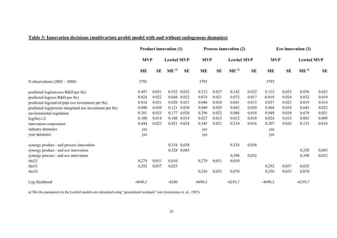
The main focus of this paper is on the innovation decisions of firms (i.e. the innovation output stage of our “Green CDM” model). Table 3 presents the results for the model that uses three types of innovations: 1) product innovation, 2) process innovation and 3) eco innovation. We report two types of estimates, those of a tri-variate probit model (MVP), in which the effects of common unobservable variables are captured by correlations between the error terms of the three equations, and a simultaneous trivariate probit model with endogenous dummies, our model (3) in-spired by Lewbel (2007), in which in addition synergies between the three types of innovations are estimated.11 The Lewbel MVP model nests the MVP model and is preferred to the latter by the likelihood ratio test. We shall therefore base the discus-sion on the Lewbel MVP estimates.

10 The coefficient estimates are available upon request. 11 Because these variables are at the center of interest, we only present marginal effects (ME’s) for the four investment types, the regulation variable, size and innovation cooperation.

26

Table 3: Innovation decisions (multivariate probit model with and without endogenous dummies)

Product innovation (1) Process innovation (2) Eco innovation (3)

MVP Lewbel MVP MVP Lewbel MVP MVP Lewbel MVP

ME SE ME a) SE ME SE ME a) SE ME SE ME a) SE

N observations (2002 – 2008) 3793 3793 3793

predicted log(non-eco R&D per fte) 0.497 0.031 0.552 0.032 0.212 0.027 0.142 0.022 0.123 0.032 0.076 0.023predicted log(eco R&D per fte) 0.024 0.022 0.048 0.022 0.074 0.021 0.072 0.017 -0.019 0.024 0.032 0.019predicted log(end-of-pipe eco investment per fte) 0.016 0.021 0.020 0.021 0.046 0.020 0.041 0.013 0.037 0.023 0.019 0.014predicted log(process integrated eco investment per fte) 0.090 0.030 0.121 0.030 0.049 0.029 0.042 0.020 0.064 0.034 0.045 0.022environmental regulation 0.301 0.023 0.177 0.026 0.296 0.022 0.088 0.018 0.949 0.030 0.679 0.021log(fte) t-2 0.100 0.014 0.108 0.014 0.027 0.013 0.012 0.010 0.024 0.015 0.003 0.009innovation cooperation 0.444 0.023 0.421 0.024 0.345 0.021 0.214 0.016 0.207 0.026 0.153 0.018industry dummies yes yes yesyear dummies yes yes yes

synergy product - and process innovation 0,334 0,038 0,334 0,038synergy product - and eco innovation 0,328 0,045 0,328 0,045synergy process - and eco innovation 0,398 0,032 0,398 0,032rho21 0,279 0,031 0,010 0,279 0,031 0,010rho31 0,292 0,037 0,025 0,292 0,037 0,025rho32 0,356 0,033 0,078 0,356 0,033 0,078

Log likelihood -4690,3 -6240 -4690,3 -6239,7 -4690,3 -6239,7

a) The rho parameters in the Lewbel models are calculated using “generalized residuals” (see Gourieroux et. al., 1987).

27

All eco-investment inputs seem to contribute to the three types of innovation output, except that end-of-pipe investment is insignificant for explaining the deci-sion to innovate in products and only weakly significant for the decision to innovate environmentaly. The latter result corroborates the conclusion of Rennings and Rex-häuser (2010) that the contribution of end-of-pipe investment to dynamic efficiency (and in particular product innovation) is limited.

By contrast, process integrated eco investment seems to contribute to every type of innovation output. For product innovation the marginal effect of process integrated eco investment even exceeds the contribution of eco R&D investment. By contrast, the picture for process innovation output is the other way around. However, these differences are minor after taking into account the standard errors of the esti-mated marginal effects. It can be noticed that the contribution of any type of eco investment to the usual innovation outputs considered in the mainstream of the in-novation literature (i.e. technological product - and process innovation) is relatively modest compared to the contribution of non-eco R&D inputs.

Non-eco R&D remains the most important variable for explaining technologi-cal innovations even after including eco innovation as a separate type of innovation output and after accounting for the three types of eco investment as additional inputs into innovation. Non-eco R&D is especially influential for product innovation. Non-eco R&D investment even contributes to eco innovation output more so than other types of investment, although the difference with other types of eco investment is rather small compared to the difference in their respective contributions for product – and process innovation (technological innovation).

Our results also show that innovation cooperation increases the incidence of all three types of innovation modes but that size only “matters” for product innova-tion: its coefficient is insignificant for process and eco innovation output.

Most interestingly, our results show that environmental considerations influ-ence the incidence of all three innovation modes. Responses of firms to existing and anticipated ER seem to increase the probability of adopting product -, process - and eco innovations, as the estimate of the regulation variable is significantly positive for any of the three types of innovation output. In particular, the economic signifi-cance of the contribution of ER to eco innovation output is very sizeable. The pres-ence of ER increases by 68 percentage points the occurrence of eco-innovation, by 9 percentage points the occurrence of process innovation and by 18 percentage points that of product innovations. In other words, in addition to the indirect effect of ER on innovation investment, there is also an important direct effect of ER on the inci-dence of each of the three types of innovation. We consider this last result as a strong corroboration of the weak version of the PH.

Finally, the estimates clearly point out a synergy between the three types of innovation, synergy with respect to a latent profit function. Any type of innovation increases the profitability of adopting another type of innovation. In particular, eco and non-eco innovations reinforce each other. There is no direction of causality in this synergy effects. Eco innovation can take the form of product or process innova-

28

tions, i.e. reduce the environmental impact in producing goods or services or lead to new products or services that are less polluting or energy-consuming. Conversely, new products or processes often take the form of eco-innovations.12

5.3 Productivity

This section looks into the productivity impact of applying different types of innovation, in particular eco-innovations, i.e. indirectly it examines the strong ver-sion of the PH. Because much of the discussion of the PH is concerned with the impact of ER on TFP we decided to use (value added) labor productivity (LP) and to look at the contributions of different innovation combinations to the (residual) TFP component of labor productivity. Do environmental regulations also affect an eco-nomic performance measure like total factor productivity?

Table 4_Productivity regressions

Method OLS GMM a)

Dependent variable LP LP

coeff. SE coeff. SElog(K/L) 0.206 0.010 0.202 0.014log(L) 0.067 0.034 0.076 0.017ecoR&D per fte t-1 0.341 0.065 0.244 0.099eco end-of-pipe investment per fte t-1 -0.016 0.008 -0.020 0.012eco process integrated investment per fte t-1 -0.014 0.014 -0.022 0.039environmental regulation (dummy) 0.016 0.029 0.070 0.063d001 0.001 0.042 -0.164 0.165d010 -0.130 0.050 -0.602 0.790d011 -0.010 0.044 0.462 0.327d100 0.082 0.036 0.721 0.370d101 0.032 0.039 0.554 0.318d110 0.008 0.042 -0.224 0.522d111 0.006 0.034 0.051 0.107_cons 3,313 0.051 3.259 0.090Year dummies yes YesIndustry dummies yes YesR2 0.278Wald Chi2 447.9P-value Hansen’s J statistics 0.08N 2062 2021a) Instruments used: eco R&D per fte in t-1, eco end-of-pipe investment per fte in t-1, eco-process integrated investment in t-1, environmental regulations, year and industry dummies, log(age), log(age) squared, innovation propensities, log(K/L) and log(L) one year lagged.

12 The observed frequencies of innovation adoptions are as follows for the sample used in table 3: d000=39%, d001=7%, d010=3%, d011=6%, d100=8%, d101=11%, d110=6% and d111=20%, where the first index refers to product innovation, the second to process innovation and the third to eco inno-vation, a zero denoting no innovation and a one the presence of innovation. The frequencies are very similar for the sample used in table 4.

29

We first present the results of a simple OLS regression that explains labor productivity differences between firms and over time with the help of the innovation dummies representing the innovation combinations observed in the data. Besides industry and year dummies, the regressions control for the beginning-of-period eco-investment intensities (i.e. eco-R&D, end-of-pipe eco-investments, and process-integrated eco-investments), the presence of environmental regulations, the capital-labor ratio and a scale effect. The residual represents TFP, and therefore the effects of eco-investments, environmental regulation and the innovation combination dum-mies can be interpreted as affecting TFP.

The OLS estimates presented in table 4 show that there is some evidence of modest scale economies: the labor and capital output elasticities add up to 1.076, the capital elasticity of output being estimated at 0.2. Eco-R&D exerts a substantial positive direct contribution to productivity besides the effect exerted via the innova-tion dummies included in the models. The direct effect of end-of-pipe eco invest-ments is negative while the eco process-integrated investments are not significant. Environmental regulation does not make a statistically significant difference. Among the innovation combinations, only one, innovating in products only (d100), affects TFP more than the reference scenario of on innovation.13

However, a drawback of the OLS estimation is that the innovation dummies are not fully exogenous. This assumption contradicts our efforts so far to correct for endogeneity in our structural model. We have modeled innovation as a separate pro-duction process and this makes the exogeneous treatment of the innovation dummies implicitly made in the OLS estimation inadequate from a methodological point of view. To circumvent these shortcomings we re-estimated the productivity equation using the GMM instrumental variables (IV) method. The GMM estimation uses the predicted propensities derived from the innovation output model as instruments in addition to the logarithms of the firms’ age and its square, and the lagged values of capital intensity and labor input. The results of the GMM estimation clearly show that the endogeneity of the innovation dummies is an important issue. Although the coefficients have different magnitudes, in essence they convey the same story. No innovation combination anymore has a statistically higher or lower contribution to TFP than the case of no innovation. Eco-R&D continues to have a positive and sig-nificant direct effect on TFP whereas the other eco investments and environmental regulation do not have a significant effect. Hence, like the study by Lanoie et al. (2011), our results do not support the strong version of the PH. Since no innovation combination increases TFP and since the only direct eco-investment effect on TFP goes via eco-R&D, the incidence of which is not affected by ER, we conclude that the total effect of ER on TFP is insignificant.

In order to test for complementarity and substitutability between innovation modes in terms of their effects on TFP performance, we need to test the inequality restrictions derived in section 3.4. The Kodde-Palm (1986) test statistics used in the Mohnen-Röller (2005) test procedure can be calculated by re-estimating for every

13All combinations are to be compared with the reference combination (D000), whose contribution is included in the constant term of the regressions.

30

pair of innovation modes the GMM model under inequality constraints and then performing a Wald test of the difference between the constrained and unconstrained estimates. We run two types of tests: once we test for the null hypothesis of com-plementarity and once for the null hypothesis of substitutability.

The results reported in Table 5 show that a 5 % level of significance eco in-novation is complementary, and definitely not substitute, to product as well as to process innovation, and that product and process innovations are substitutes and definitely not complements. Only the complementarity in the introduction of product and process innovations is no longer present when it comes to synergy in reaching higher levels of TFP. We hence do not find the crowding-out of technological inno-vations by environmental innovations that Marin (2012) reported for Italian firms using a model similar to ours but patent counts instead of innovation occurrences as a measure of innovation output.

6. Conclusion

This paper presents a new attempt to investigate the validity of the Porter hy-pothesis using a more structural modeling approach than mostly used up to now in the mainstream of empirical research on this topic. We apply a “Green type of CDM” innovation model to a very comprehensive data set built after matching four surveys. The use of detailed data on energy use and energy tariff structures enables us to construct marginal energy prices at the firm level. These data and the firm-level data on several types of eco investments, non-eco R&D investment and re-sponses to environmental regulations (ER) are used to assess the importance of en-ergy price incentives and ER for the different stages of the innovation process con-

Table 5 Results for testing super- and sub-modularity using the LP equation

I) H0: complementarity Combination Product-Process Product-Eco Process-EcoKodde-Palm Test Statistics 2,974 0,032 9,409-E-5

II) H0: substitutability Combination Product-Process Product-Eco Process-EcoKodde-Palm Test Statistics 5,588E-05 2,930 4,982

The lower bound for the Kodde-Palm test for 2 degrees of freedom is 1.642 at 5% level of significance and 3.808 at the 10% level of significance. The respective upper bounds are 2.706 and 5.138. The null hypothesis is not rejected if the test statistic falls below the lower bound and is rejected if it falls above the upper bound. In between the two bounds the test is inconclusive.

31

sidered in the CDM innovation model. Furthermore, our model tests for the exis-tence of synergies in the occurrence of, and in the effect on total factor productivity (TFP) of product, process and eco innovations.

Our empirical results strongly corroborate the weak version of the PH. This conclusion can be broken down into several parts: 1) besides environmental invest-ment subsidies and the pre-existing dependence of firms on energy use, marginal energy prices (including carbon taxes) are among the most important determinants of eco investment 2) there is a significantly positive contribution of eco investment to the propensity of introducing environmental innovations 3) existing or anticipated environmental regulations increase the propensity of firms to innovate environmen-tally but also in products and processes, and 4) the results clearly point to comple-mentarities in the introduction of product-, process- and eco innovations, and to synergy between technological and environmental innovations in reaching higher levels of TFP. All this leads to the conclusion that environmental considerations, be it in the form of government regulations or in the form of market pressures, seem to be an important element in the decision making of firms to invest in R&D and eco investments and play a major role in the introduction of different types of innova-tion, in particular eco innovations.

However, we cannot conclude anything concerning the strong version of the PH, because, on the one hand, the three measures of innovation output do not seem to contribute significantly to TFP performance, and hence environmental regulations have no indirect effect on TFP, and, on the other hand, the only eco-investment that contributes directly to TFP, eco R&D, is not affected by environmental regulations. Maybe more time is needed for the effects of environmental regulations to show up in economic performances. Future work on dynamic modeling with sufficiently long time lags between innovation and productivity might reveal a different picture.

References

Acemoglu, Daron, Philippe Aghion, Leonardo Bursztyn and David Hemous, 2012, “The environment and directed technical change”. American Economic Review, Vol. 102(1), pp. 131–166.

Ambec, Stefan and Philippe Barla, 2002, “A theoretical foundation of the Porter Hypothesis”. Economic Letters, Vol. 75, pp. 355–360.

Ambec, Stefan and Philippe Barla, 2006, “Can environmental regulation be good for Business? An assessment of the Porter hypothesis”. Energy Studies Review, Vol. 14, Issue 2, Article 1.

Ambec, Stefan, Mark A. Cohen, Stewart Elgie and Paul Lanoie (2011), “The Porter hypothesis at 20”, Discussion Paper 11-01, Resources for the Future.

Amemiya, Takeshi, 1984, “Tobit models: a survey”. Journal of Econometrics, Vol. 23, pp. 3–62.

32

Cainelli, G., G. Marin and M. Mazzanti, 2010, “ICT investment, eco-innovations and environmental efficiency”. Paper presented at ZEW Conference “The Econom-ics of Green IT”, Mannheim Germany.

Cerin, Pontus, 2006, “Bringing economic opportunity into line with environmental influence: A discussion on the Coase theorem and the Porter and van der Linde hy-pothesis”. Ecological Economics, Vol. 56, pp. 209–225.

Chung, Y. H., R. Färe and S. Grosskopf, 1997, “Productivity and undesirable out-puts: A directional distance function approach”. Journal of Environmental Manage-ment, Vol. 51, pp. 229–240. Cappellari, Lorenzo and Stephen P. Jenkins, 2003, “Multivariate Probit regression using simulated maximum likelihood”. The Stata Journal, Vol.3, No3, pp. 278–294.

Cappellari, Lorenzo and Stephen P. Jenkins, 2006, “Calculation of multivariate normal probabilities by simulation, with applications to maximum simulated likeli-hood estimation”. The Stata Journal, Vol.6, No 2, pp. 156–189.

Constantatos, Christos and Markus Hermann, 2011, “Market inertia and the intro-duction of green products: Can strategic effects justify the Porter hypothesis?”. En-vironmental and Resource Economics, Vol. 50, pp. 267–284.

Crépon, Bruno, Emmanuel Duguet and Jacques Mairesse, 1998, “Research, innova-tion and productivity: an econometric analysis at the firm level. Economics of Inno-vation and New Technology, Vol. pp. 115–158.

Desrochers, Pierre, 2008, “Did the invisible hand need a regulatory glove to develop a green thumb? Some historical perspective on market incentives, win-win innova-tions and the Porter hypothesis”. Environmental and Resource Economics, Vol. 41, pp. 519–539.

Domazlicky, Bruce R. and William L. Weber, 2004, “Does environmental protec-tion lead to slower productivity growth in the chemical industry?” Environmental and Resource Economics, Vol. 28, pp. 301–324.

Gans, Joshua, S., 2012, “Innovation and climate change policy”. American Eco-nomic Journal, Vol. 4(4), pp. 125–145.

Gourieroux, Christian, Alain Monfort, Eric Renault and Alain Trognon, 1987, “Generalized residuals”. Journal of Econometrics, Vol. 34, pp. 5–32.

Heckman, James, J., 1978, “Endogenous variables in a simultaneous equation sys-tem”. Econometrica, Vol. 46, No 4, pp. 931–959.

Horbach, Jens and Klaus Rennings, 2012, “Environmental innovation and employ-ment dynamics in different technology fields – An analysis based on the German Community Innovation Survey 2009”. ZEW Discussion Paper No. 12-006. ZEW (Centre for European Economic Research), Mannheim, Germany.

33

Jaffe, Adam, B., Richard G. Newell and Robert N. Stavins, 2002, “Environmental policy and technological change”. Environmental and Resource Economics, Vol. 22, pp. 41–69.

Jaffe, Adam, B., Richard G. Newell and Robert N. Stavins, 2003, “Technological change and the environment”. Chapter 11 in: Handbook of Environmental Econom-ics, Vol. 1. Edited by K. G Mäler and J. R. Vincent. Elsevier Science Publishers.

Jaffe, Adam and K. Palmer, 1997, “Environmental regulation and innovation: A panel data study”, Review of Economics and Statistics, Vol. 79, No. 4, pp. 610-619.

Kemp R. (2011), Eco-Innovation: definition, measurement and open research issues, Economia Politica, n. 1, in press. Kodde, David, A. and Franz Palm, 1986, “Wald criteria for jointly testing equality and inequality restrictions”. Econometrica, Vol. 54, No. 5, pp. 1243–1248. Kretschmer, Tobias, Eugenio J. Miravete and José C. Pernías (2012), “Competitive pressure and the adoption of innovations”. American Economic Review, Vol 102, No. 4, pp.1540-1570.

Kriechel, Ben and Thomas Ziesemer, 2009, “The environmental Porter hypothesis: Theory evidence and a model of timing of adoption”. Economics of Innovation and New Technology, Vol. 18, No 3, pp. 41–69.

Lanoie, Paul, Jérémy Laurent-Luccheti, Nick Johnstone and Stefan Ambec, 2011, “Environmental policy, innovation and performance: New insights on the Porter hypothesis”. Journal of Economics and Management Strategy, Vol. 20, No. 3, pp. 803-842.

Lewbel, Arthur, 2007, “Coherency and completeness of structural models containing a dummy endogenous variable”. International Economic Review, Vol. 48, No 4, pp. 1379–1392.

Marin, Giovanni, 2012, “Do eco-innovations harm productivity growth through crowding out? Results on an extended CDM model for Italy”. IMT Lucca EIC work-ing paper series 03.

McFadden, D. L., 1973. “Conditional logit analysis of qualitative choice behavior,” in Frontiers in Econometrics (P. Zarembka, ed.). New York: Academic Press.

Milgrom, Paul and John Roberts, 1990, “The economics of modern manufacturing, technology, strategy and organizations”. American Economic Review, Vol. 80, pp. 511–528.

Milgrom, Paul and John Roberts, 1995, “Complementarities and fit. Strategy, struc-ture and organizational change in manufacturing”. Journal of Accounting & Eco-nomics, Vol. 19, pp. 179–208.

Miravete, E. and J. Pernías (2006). “Innovation complementarity and scale of pro-duction”. Journal of Industrial Economics, Vol. 54, pp. 1-29.

34

Mohnen, Pierre and Lars-Hendrik Röller, 2005, “Complementarities in innovation policies”. European Economic Review, Vol. 49, pp. 1431–1450.

Mohr, Robert D., 2002, “Technical change, external economies, and the Porter hy-pothesis”. Journal of Environmental Economics and Management, Vol. 43, pp. 158–168.

Muller, Nicholas Z., Robert Mendelsohn and William Nordhaus, 2011, “Environ-mental accounting for pollution in the United States economy”. American Economic Review, Vol. 101, pp. 1649–1675.

Palmer Karen, Wallace E. Oates and Paul R. Portney, 1995, “Tightening environ-mental standards: The benefit-cost or no-cost paradigm?”. Journal of Economic Per-spectives, Vol. 9 (4), pp. 119–132. Polder, Michael, George van Leeuwen, Pierre Mohnen and Wladimir Raymond, 2010, “Product- process and organizational innovation: drivers, complementarity and Productivity effects”. UNU-MERIT Working Paper 2010-035, UNU-MERIT, Maastricht.

Popp, David, Richard G. Newell and Adam B. Jaffe, 2002, “Energy, the environ-ment, and technological change”. Chapter 21 in: Handbooks in Economics, Vol. 2. Elsevier Science Publishers.

Porter, Michael, E.,1991, “America’s green strategy”. Scientific American, Vol. 264, pp. 168.

Porter, Michael, E and Claas van der Linde, 1995, “Toward a new conception of the environment-competitiveness relationship”. The Journal of Economic Perspectives, Vol. 9, No 4, pp. 97-118.

Rennings, Klaus and Sascha Rexhäuser, 2010, “Long-term impacts of environmental policy and eco-innovative activities of firms”. ZEW Discussion Paper No. 10-074. ZEW (Centre for European Economic Research), Mannheim, Germany.

Rennings, Klaus and Christian Rammer, 2010, “The Impact of Regulation-driven environmental innovation on innovation success and firm performance”. ZEW Discussion Paper No. 10-065. ZEW (Centre for European Economic Re-search), Mannheim, Germany.

Rexhäuser, Sascha and Christian Rammer, 2011, “Unmasking the Porter hypothesis: Environmental innovations and firm-profitability”. ZEW Discussion Paper No. 11-036. ZEW (Centre for European Economic Research), Mannheim, Germany.

Tamer, Elie, 2003, “Incomplete simultaneous discrete response model with multiple equilibria”. The Review of Economic Studies. Vol. 70, No 1, pp. 147–165.

Train, Kenneth, 2003, Discrete Choice Methods with Simulations. Cambridge Uni-versity Press, Cambridge UK.

35

Wagner, Marcus, 2003, “The Porter hypothesis revisited: A literature review of theoretical models and empirical tests”. Research Memorandum Center for Sustain-ability Management (SM) University of Lüneburg. Lüneburg, Germany.

Wooldridge, J. M., 2002, Econometric Analysis of Cross Section and Panel Data. The MIT Press, Cambridge Massachusetts, Cambridge USA.

36

Appendix A: List of variables used in this study

a) Data Survey Environmental Costs of Firms (ECF)

hef_to : total environmental levies (Eu) inv_p_t : environmental investments process integrated (1000 Eu) inv_to_t : environmental investments "end-of-pipe" (1000 Eu) inv_to : total environmental investment in current prices (1000 Eu) subkl_to : total environmental subsidies received (1000 Eu) eco_subs : dummy for eco subsidies >= 5000 Eu sh_hef : share of environmental levies in total environmental exploitation costs sh_proc_inv : share process integrated investment in total environmental investment sh_subs : share environmental subsidies in total environmental costs sh_pi_inv : share process integrated investment in total environmental investment pimi : price deflator total environmental investment zrv : total expenditure on environmental R&D (1000 Eu) erd : environmental R&D in constant prices (1000 Eu) ecoinput : environmental innovation input (R&D and investment; 1000 Eu) inv_eco : total environmental innovation input in constant prices

b) Data Energy Statistics Survey (ES) v_aardgas : total volume of gas used (1000 m3) v_electra : total volume of electricity used (1000 Kwh) prijs_electra : marginal price electricity based on tariff structure electrici- ty prijs_gas : marginal price gas based on tariff structure gas mp : marginal energy prices per TJ (after converting gas and electricity in TJ's) sh_tax : share marginal tax in gross marginal energy price sh_tax_ex : marginal tax as a percentage of energy prices net of taxes mean_tax : mean energy tax per TJ

Energy data Production Statistics Survey (PS) pg_mean : unit values gas (Euro/m3) PS pe_mean : unit value electricity (Euro/Kwh) PS aardgas : consumption of gas used (1000 Eu) electriciteit : consumption of electricity used(1000 Eu) uv : unit values total energy input (Euro per TJ) pi_energie : firm-specific price index based on unit values per TJ sh_energy : energy cost share (derived from ES and PS)

c) Innovation data (CIS)

1) Inputs into innovation: rrdinx : in-house R&D expenditure in current prices, cen- sored (1000 Eu) rrdexx : outsourced R&D expenditure in current prices, censored (1000 Eu)

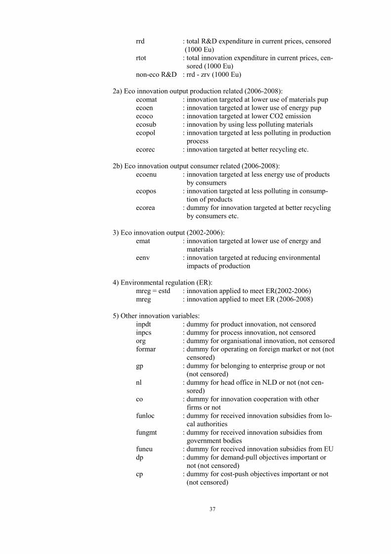
37

rrd : total R&D expenditure in current prices, censored (1000 Eu) rtot : total innovation expenditure in current prices, cen- sored (1000 Eu) non-eco R&D : rrd - zrv (1000 Eu)

2a) Eco innovation output production related (2006-2008): ecomat : innovation targeted at lower use of materials pup ecoen : innovation targeted at lower use of energy pup ecoco : innovation targeted at lower CO2 emission ecosub : innovation by using less polluting materials ecopol : innovation targeted at less polluting in production process ecorec : innovation targeted at better recycling etc.

2b) Eco innovation output consumer related (2006-2008): ecoenu : innovation targeted at less energy use of products by consumers ecopos : innovation targeted at less polluting in consump- tion of products ecorea : dummy for innovation targeted at better recycling by consumers etc.

3) Eco innovation output (2002-2006): emat : innovation targeted at lower use of energy and materials eenv : innovation targeted at reducing environmental impacts of production

4) Environmental regulation (ER): mreg = estd : innovation applied to meet ER(2002-2006)

mreg : innovation applied to meet ER (2006-2008)

5) Other innovation variables: inpdt : dummy for product innovation, not censored inpcs : dummy for process innovation, not censored org : dummy for organisational innovation, not censored formar : dummy for operating on foreign market or not (not censored) gp : dummy for belonging to enterprise group or not (not censored) nl : dummy for head office in NLD or not (not cen- sored) co : dummy for innovation cooperation with other firms or not funloc : dummy for received innovation subsidies from lo- cal authorities fungmt : dummy for received innovation subsidies from government bodies funeu : dummy for received innovation subsidies from EU dp : dummy for demand-pull objectives important or not (not censored) cp : dummy for cost-push objectives important or not (not censored)

38

d) Production Statistics Survey (PS)

fte : employment (in full-time equivalent) nv : value of total turnover (1000 Eu ) nq : value of gross output (1000 Eu) nm : value of total intermediate inputs (E + M + S, 1000 Eu) va : value added (nq – nm) bedrlst341000 : total cost of energy use (1000 Eu) bedrlst310000 : total cost of production (1000 Eu) depr : total depreciation costs (1000 Eu, proxy for capital inputs) sh_energy : cost share energy (bedrlst341000/bedrlst310000)

39

Appendix B: The likelihood function for the Lewbel Model

In this appendix we describe the derivation of the likelihood function for our

empirical application. The computational complexities arise due to the requirement to have full error support over all possible combinations (strategy choices). Refer-ring to equations (3) in the text, there are eight possible combinations of the three

types of innovation. Thus, for every adopted combination, seven )12( −N compari-

sons are at stake. To keep things tractable we will focus on strategy (3a). Adopting strategy (3a), no innovation at all (thus all comparisons are against zero profits), yields the following set of inequalities: 14

dUBUBxVV 33333)1,0,0()0,0,0( ≡=′−<⇒⇔ βε

dUBUBxVV 2121222)0,1,0()0,0,0( ≡=′−<⇒⇔ βε

32222323

33222)1,1,0()0,0,0( εεαββε −≡=−−′−′−<⇒⇔ dUBUBxxVV

dUBUBxVV 1111111)0,0,1()0,0,0( ≡=′−<⇒⇔ βε (B1)

21212212

22111)0,1,1()0,0,0( εεαββε −≡=−−′−′−<⇒⇔ dUBUBxxVV

31313313

33111)1,0,1()0,0,0( εεαββε −≡=−−′−′−<⇒⇔ dUBUBxxVV

2313123322111)1,1,1()0,0,0( αααβββε −−−′−′−′−<⇒⇔ xxxVV

32141432 εεεε −−≡=−− dUBUB

In (B1) we make a distinction between the deterministic part (indicated by dijUB ) and

the stochastic part of the right-hand side (RHS). Notice that, for N = 3, we have one inequality involving ,3ε two involving 2ε and four involving .1ε Any coherency prob-

lem is lifted if we take the minimum of the upper bounds of the inequalities on the right-hand sides.

So we replace the inequalities for 2ε by ),min( 322212 εε −< dd UBUB and similarly

for the inequalities involving 1ε :

).,,,min( 3214313212111 εεεεε −−−−< dddd UBUBUBUB

The (joint) probability for the case of no innovation at all is given by

14 We use superscripts to denote the sum of ijα and jiα . Thus, .jiijij ααα +=

40

}0,0,0Pr{ 321 === yyy

),,,min(Pr{ 3214313212111 εεεεε −−−−<= dddd UBUBUBUB

}&),min(& 33322212ddd UBUBUB <−< εεε

),,,min(Pr{ 3214313212111 εεεεε −−−−<= dddd UBUBUBUB

}&),min(| 33322212ddd UBUBUB <−< εεε

X }|),min(Pr{ 33322212ddd UBUBUB <−< εεε

X }Pr{ 33dUB<ε .

Similar expressions can be derived for the other combinations of strategies. The expressions involve conditioning upon unobservable variables to enable GHK simu-lation for evaluating the integration bounds in the likelihood function. For example for P(0,0,0), the likelihood function is given by

23)3|322,21min(

23

33 )|()( εεεεεεε

dfdfdUBdUBdUB

∫∫−

∞−∞−∗

,),|( 132)3,2|3214,313,212,11min(

1 εεεεεεεεεε

dfdUBdUBdUBdUB

∫−−−−

∞−∗

where f(.) stands for the density function of the normal distribution.