Revisiting the determinants of non-farm - GRADE
98
Transcript of Revisiting the determinants of non-farm - GRADE


Revisiting the determinants of non-farm income in the Peruvian Andes in a context of intraseasonal climate variability and spatially
widespread family networks


Avances de Investigación 34
Revisiting the determinants of non-farm income in the Peruvian Andes in a context of intraseasonal climate variability and spatially
widespread family networks
Carmen Ponce1
1 Associate Researcher at the Group for the Analysis of Development (GRADE).This paper is part of my doctoral dissertation at the Pontificia Universidad Católica del Peru. I am grateful to my advisors Javier Escobal and Javier Iguíñiz for their insightful comments and encouragement. I also thank seminar participants at the 2017 Conference of the Canadian Economics Asosociation (June 2017) and seminar participants at the Group for the Analysis of Development (August 2017), for their contributions to an early version of the study. Finally, I am thankful to Lorena Alcazar for her useful comments and suggestions. Remaining errors are, of course, my responsibility.

GRADE´s research progress papers have the purpose of disseminating the preliminary results of research conducted by our researchers. In accordance with the objectives of the institution, their purpose is to perform rigorous academic research with a high degree of objectivity, to stimulate and enrich the debate, design and implementation of public policies. The opinions and recommendations expressed in these documents are those of their respective authors; they do not necessarily represent the opinions of their affiliated institutions. The authors declare to have no conflict of interest related to the current study's execution, its results, or their interpretation. The study and publication are funded by the International Development Research Centre, Canada, through the Think Tank Initiative.
Lima, July 2018
GRADE, Group for the Analysis of DevelopmentAv. Almirante Grau 915, Barranco, Lima, PeruPhone: (51-1) 247-9988Fax: (51-1) 247-1854www.grade.org.pe
The work is licensed under a Creative Commons Attribution-NonCommercial 4.0 International Research director: Santiago CuetoEdition assistance: Diana Balcázar TafurCover design: Elena GonzálezDesign of layout: Amaurí Valls M.

Index
Abstract 7
Introduction 9
1. Literature review on rural households’ income diversificationinto non-farm activities 15
2. The model 25
3. Data 31
4. Results and discussion 371. A descriptive look at the role of intraseasonal climate variability
and strong distant ties on households’ diversification strategies 372. Estimation results 51
5. Conclusions and final remarks 63
References 67
Appendix 77


ABSTRACT
Non-farm income sources are increasingly important in the develop-ing world, representing up to 50 percent of average rural household income. Although there is a vast literature on the determinants of rural households’ strategies for income diversification, two factors associat-ed with long term transformations and common to many developing countries, have not yet been integrated into the analysis: (i) the role of intraseasonal climate variability (affected by climate change), and (ii) the role of family networks located in distant areas (increasinglyimportant given population displacement due to the internal conflictand increasing connectivity via roads and communications). Whereasan increase in climate variability entails an increase in risk and vulner-ability for farm activities, family networks located in distant regions(that do not share the local climate or market shocks) may becomea key asset for managing risk and fostering income opportunities (aslong as they convey information and opportunities that are not avail-able through local networks). Given the market imperfections that arecommon in developing rural areas—especially those related to climaterisk management—explicit consideration of both factors is key to un-derstanding rural households’ diversification strategies. The study aimsto contribute to this pending agenda, investigating the role of thesetwo factors on a household’s income diversification into non-farm ac-tivities in the Peruvian Andes, a mountain region with large intrasea-sonal climate variability and limited but increasing spatial connectivity,

8 Revisiting the determinants of non-farm income in the Peruvian Andes
where the rural population was severely affected by the internal conflict that took place in the country during the eighties and nineties.
Two economic outcomes are modeled: the share of non-farm working hours and the share of non-farm labor income. We find that, controlling for other assets and environmental conditions, households with distant but strong networks tend to diversify more into non-farm activities (the results suggest that there is a substitution effect between distant strong and weak ties). Increases in intraseasonal climate vari-ability (proxied by temperature range during the main crop growing season) induce rural households to increase the relative share of non-farm income and working hours. The analysis shows heterogeneous effects within the Andean region. While in the Northern region and colder areas in the Central Andean region (below 13˚C during the crop growing season) an increase in intraseasonal climate variability induces rural households to increase non-farm income-generating activities, the Southern region shows no significant impact. Further analysis is needed to understand whether this lack of effect is explained by farm-related responses.
These results suggest that interventions focused on helping farm-ers cope with climate change should consider not only farm activities but skills and assets required to access non-farm occupations as well. A type of asset that is usually neglected by development projects is households’ distant networks, which can actually play a role in risk management strategies, according to our results.
INTRODUCTION
Non-farm income sources are increasingly important, representing between one third and one half of rural households’ income in devel-oping countries (Reardon et al. 2007).2 Previous studies suggest that non-farm income can help reduce poverty and strengthen investment in agricultural activities; however, evidence shows that this positive linkage between non-farm activities and poverty reduction depends on market dynamism (Reardon, Berdegué, & Escobal 2001; Lanjouw 2007). The literature also shows the important role that education and access to infrastructure and markets, as well as the elimination of market failures, have in facilitating access to non-farm high-paying jobs for rural households in the developing world (Himanshu et al. 2013, Lanjouw & Murgai 2009, Reardon et al. 2007, de Janvry & Sa-doulet 2001, among others). Although these studies have analyzed the determinants of non-farm income, two common features in most de-veloping countries that are associated with current trends have not yet been integrated into the analysis: (i) the role of intraseasonal climate variability (affected by climate change)3, and (ii) the role of family
2 Hazell, Haggblade, and Reardon (2007: 84) compile evidence from several studies and show increases of rural non-farm income shares among farm households from 17% to 39% between 1978-80 to 1997 in China, from 22% to 84% between 1950 and 1987 in Japan, from 18% to 46% between 1971 to 1991 in South Korea, from 45% to 78% between 1970 and 1987 in Taiwan, and from 35% to 46% between 1976 and 1986 in Thailand.
3 According to the IPCC (2014b), climate refers to “the average weather, or more rigorously, as the statistical description in terms of the mean and variability of relevant quantities over a period of time ranging from months to thousands or millions of years. The classical

10 Revisiting the determinants of non-farm income in the Peruvian Andes
networks located in distant areas (increasingly important given popu-lation displacement during the internal conflict and increasing road and communications connectivity). This study, focused on Peruvian Andean farmers, aims to contribute to this pending agenda.
The Peruvian Andean region is particularly interesting for two reasons. First, according to the IPCC (2014a), the Andean region has been severely affected by climate change, mostly due to the increase in temperature—accelerating the glacier retreat—and the heterogeneous changing patterns in precipitation. Although Andean farmers have historically managed to cope with climate variability, climate change has intensified and made the already variable conditions that Andean farmers face during the crop growing season less predictable (Verga-ra 2012, Postigo 2012, Valdivia et al. 2010, Escobal & Ponce 2010, among others). Second, the internal conflict that took place in Peru during the eighties and nineties affected the Andean and indigenous population (most of them farmers) disproportionately more than other groups and caused population displacement across the country (some of whom returned after the end of the war). Furthermore, the greater connectivity achieved in the last three decades has enhanced population mobility, both permanent and seasonal, and the consolidation of inter-mediate cities has fostered rural-urban socio-economic linkages (Llona, Ramirez, & Zolezzi 2004; Ponce 2010). As a result, 28% of Andean rural households in Peru have a sibling or parent living in a different province4 (56% if household head’s or spouse’s children are included).
period for averaging these variables is 30 years, as defined by the World Meteorological Organization. The relevant quantities are most often surface variables such as temperature, precipitation, and wind.” Here, I study intraseasonal climate variability, which is proxied by the 30-year average temperature range, calculated as the difference between the average maximum and the average minimum temperatures estimated for a particular trimester.
4 Peru is divided into three political-administrative levels, consisting of 25 departments, 196 provinces, and 1,867 districts.

11Introduction
This study investigates the role of intraseasonal climate variabil-ity (associated with risk and vulnerability in farm activities) and spa-tially distant family networks (potential social capital to rural house-holds) in the relative importance of non-farm income for Andean rural households. Two household economic outcomes summarize the relative importance of non-farm income sources: the non-farm labor income share (the proportion of labor income earned from non-farm activities), and the non-farm labor share (the proportion of household working hours allocated to non-farm activities). As usual in this lit-erature, non-farm activities refer to activities other than agriculture, which includes the production of crops, livestock husbandry, aquacul-ture, woodlot production, hunting, fishing, and forestry (Haggblade, Hazell, & Reardon 2007; Dirven 2004). In the Andean region, the crop production and livestock husbandry are the main components of agricultural activities. Non-farm sources of income include both wage work and self-employment.
The first hypothesis that underlies this study is that an increase in intraseasonal climate variability entails an increase in risk and vulner-ability for farm activities. As pointed out by Reardon et al. (2007), climate-related risks can push farmers into non-farm activities (which are less vulnerable to such risks). Therefore, I expect that rural house-holds tend to invest more in non-farm activities as intraseasonal cli-mate variability increases. This higher investment, controlling for other factors relevant to the household’s decision, would increase the household’s shares of non-farm income and working hours. It is worth noting that the econometric estimation requires adequately control-ling for confounding factors, including other climate conditions that are also key to households’ decisions about the mix of farm/non-farm activities. For instance, while an increase in temperature may open opportunities to grow crops that used to be unviable in certain areas,

12 Revisiting the determinants of non-farm income in the Peruvian Andes
an increase in temperature in areas with high variability may not be incentive enough to embark on production of new, more profitable crops. Thus, the estimation of the effect of intraseasonal climate vari-ability needs to account for such an interaction with average temper-ature conditions. Local economic conditions—such as local house-holds’ connections to markets, the average productivity of farm and non-farm activities, among others—may also play a role due to spill-over effects and market signaling of each sector’s expected profitabil-ity. Furthermore, institutional and socio-economic conditions such as the feasibility of increasing/decreasing land assets (through sale or rent) and in general, the local socio-economic and cultural factors mediating access to common goods and natural resources may play a role in the economic opportunities available to the rural household. To take into account these conditions, I control for relevant covariates and further explore parameter heterogeneity across the Andean Cen-tral, Southern, and Northern domains.
The second hypothesis refers to the role of distant but strong ties on the relative importance of households’ non-farm activities. A household’s strong distant ties are proxied by the household’s close family networks in distant areas (siblings or parents of the household head or spouse who live in a different province). I argue that strong distant ties may become a form of social capital as long as they can provide new information for economic activities that would other-wise be unknown to the household (new products, new markets, new technologies), and can also reduce the transaction costs involved in accessing new markets. I expect this effect to be important for both farm and non-farm activities. Nevertheless, as discussed later, distant ties may have a zero or even a negative effect in some cases. Strong distant ties may have no impact on household economic decisions if the household has a second residence close to more dynamic markets,

13Introduction
or may even be associated with lower economic outcomes when the household’s distant family is in critical need, or when the absence of strong ties in local areas is related to a systematic emigration of com-munity members that weakens traditional community strategies for coping with risk (Valdivia et al. 2010). It could also be argued that such ties may become redundant when other families in the commu-nity have strong distant ties; in other words, it may be important to have such an asset at the community level, but it eventually becomes redundant at the individual level. Given these potential complexities, the econometric specification accounts for the interaction between a household’s strong distant ties and other community households’ strong distant ties (weak ties), owning a second residence, and other household characteristics associated with a capacity to convert social capital into actual economic opportunities (education, access to pub-lic services, dependence ratio, bi-parental status, and so on).
The analysis in this study is based on the largest survey performed in Peru for rural areas, representative of rural households at the prov-ince or department level: the Provincial Survey of Rural Households (EPHR, according to its initials in Spanish). Despite the limitations that a cross-sectional analysis usually entails, this survey is the first one to provide rural household information about both income-gen-erating strategies and the location of direct family networks across the country. Furthermore, given the strong representativeness of this sur-vey, it allows for not only the estimation of province-level productiv-ity measures (rarely available) but also, more importantly, of hetero-geneous parameters for domains that show different climate patterns and socio-economic dynamics (Northern, Central, and Southern). The statistical information from EPHR is complemented by climate indicators at the district level, estimated by Ponce, Arnillas, and Es-cobal (2015). These estimates include the district’s 30-year average of

14 Revisiting the determinants of non-farm income in the Peruvian Andes
temperature range—a proxy for intraseasonal climate variability—and temperature and precipitation, as well as the change in these condi-tions between 1994 and 2012. As is usual in the literature on climate, these estimates are calculated as 30-year averages; the average from 1964-1994 represents the climate conditions faced in 1994 and the average from 1982-2012 represents the climate conditions faced in 2012. Since these estimates were intended to help analyze farm house-holds’ strategies and decisions, they are consequently constrained to the climate conditions of areas under 4,800 m.a.s.l.5, above which are biologically unviable areas (Ponce, Arnillas, & Escobal 2015). Finally, complementary information about socio-political and economic fea-tures was used to account for environmental conditions that may af-fect households’ decisions on income diversification strategies.
The document is organized into six sections, including this one. The following section presents a literature review about the determi-nants of non-farm income and rural households’ diversification strate-gies, with emphasis on the role of climate risks and vulnerabilities. Given the scarce literature on the role of spatially distant family net-works in rural households’ diversification strategies (besides their role as migration capital), I discuss the literature on the role of strong and weak ties in economic outcomes and link it to income diversification strategies employed by rural households. Section 3 summarizes the the-oretical model and the empirical specification, then Section 4 explains the data sets used in the analysis. Section 5 discusses the results in two parts—a descriptive subsection followed by the estimations’ findings. Finally, Section 6 concludes and introduces some final remarks.
5 Meters above sea level.

1. LITERATURE REVIEW ON RURAL HOUSEHOLDS’ INCOME DIVERSIFICATION INTO NON-FARM
ACTIVITIES
There is a vast literature on the increasing importance of non-farm income and the role it plays in reducing rural poverty in various de-veloping countries (Reardon, Berdegué, & Escobar 2001; Reardon et al. 2007). Based on 54 country studies published in the 1990s and 2000s, Reardon et al. (2007) argue that non-farm income accounts for 47%, 34%, and 51% of rural income in Latin America, Africa, and Asia, respectively. One of these studies, led by Escobal (2001), focuses on Peru. Escobal (2001: 502) shows that non-farm income represented 47% of labor income in the rural Peruvian Andes region in 1997 (42% and 5% from self-employment and wage employment sources, respectively).6
Reardon et al. (2007) emphasize that the factors leading rural households to diversify into non-farm activities may differ substan-tially across income groups. While some households diversify off-farm to accumulate capital, perhaps for reinvestment in agricultural tech-nology, and to grow financially (pull factors), others diversify to cope with poverty and deprivation, aiming to reduce their vulnerability to the risks and shocks usually involved in agricultural activities (push
6 The definition of non-farm employment used in these studies refers to non-agricultural activities only, thus these figures exclude contributions from agricultural wage employment, which is included in our definition of off-farm activities. In any case, the discussion that follows is valid for off-farm activities in general. Given that much of agricultural wage employment in the Andean region occurs outside of a household’s local community, labor demand for these jobs is expected to be unaffected by local climate shocks in ordinary years.

16 Revisiting the determinants of non-farm income in the Peruvian Andes
factors). In some cases, like the ejidos in Mexico, farmers with small land holdings diversify more than those with larger land to comple-ment their low farm income, due to the absence of land markets (de Janvry & Sadoulet 2001).
Building on previous studies, Reardon et al. (2007) classify the determinants of income diversification into non-farm activities into three groups: relative prices of outputs and inputs associated with each activity (incentive levels), relative risks involved in each activity in-cluding climatic and market risks (instability of incentives), and assets available to the household, including human, social, financial, organi-zational, and physical (capacity variables). Escobal (2001) emphasizes that, in an absence of efficient markets, individual and institutional constraints can further affect diversification strategies. Reardon et al. (2007) also highlight the importance of local market dynamism. A growing sector in the local environment—whether agriculture, min-ing, or tourism—drives up demand for non-farm goods and services, increasing wage employment and self-employment opportunities.
In the following two subsections I review the literature on the role of climate in diversification strategies and the role of social ties in economic outcomes, in order to identify the mechanisms through which these two variables affect rural households’ decisions to diver-sify between farm and non-farm activities.
Effect of climate on rural households’ economic outcomes
Climate conditions are arguably the main source of risk for agricul-tural activities in the Andean region. They do not only affect yields and productivity but may affect local (and sometimes regional) prices as well. Thus, several studies argue that diversifying into non-farm

17Literature review on rural households’ income diversification into non-farm activities
activities is a strategy for managing climate risk (ex ante) and coping with climate shocks (ex post) (Reardon et al. 2007, Mertz et al. 2011, Dasgupta et al. 2014). A complementary strategy for managing cli-mate risks in the Andean region is diversification of the farm’s crop portfolio (Lin 2011, Valdivia et al. 2010, Earls 1991, Figueroa 1989, Escobal & Ponce 2012).
Reardon et al. (2007) propose a conceptual framework for un-derstanding the mechanisms underlying the push factors that induce poor households to diversify into non-farm activities. They point out four push factors associated with climate conditions and risks. First, the seasonal nature of agricultural activities is characterized by pe-riods with very low farm activity. When farm income cannot cover the household’s needs for the whole year, households need to allocate their remaining working time and resources to pursue other income-generating activities to complement farm income. Second, unexpect-ed extreme climatic events like droughts or hail may severely affect farm income and force households to transitorily embark on off-farm7 activities to compensate for the loss of on-farm income (such as farm wage employment in a different region unaffected by the climate shock, or non-farm activities). Third, less transitory changes in cli-mate conditions, or other key factors such as soil quality or market conditions, may negatively affect households’ farm activities and call for a more permanent change in income-generating strategies, away from agriculture self-employment. Finally, a fourth push factor, asso-ciated with the second one, is that credit or insurance market failures
7 On-farm activities refer to farm activities undertaken on the household’s own farm. In contrast, off-farm activities include farm wage employment, and non-farm wage and self-employment. The present study is focused on the farm/non-farm divide (farm: agricultural or farm wage and self-employment; non-farm: non-agricultural wage and self-employment).

18 Revisiting the determinants of non-farm income in the Peruvian Andes
push households to find alternative ways to self-insure against climate shocks or fund purchases of farm inputs. The authors argue that weak land and labor markets may also induce households to diversify into non-farm activities. These mechanisms are implicitly taken into con-sideration in the model in Section V.
Households’ perceptions of climate and their expectations with regards to the weather conditions that will be prevalent in the sowing-growing period are key to their decisions about the resources they in-vest in farm and non-farm activities in a particular year. They are also important for deciding whether to make a more substantial investment in farm or non-farm activities, foreseeing a longer term involvement in such activity. The potential mismatch between their expectations and the actual conditions, of course, is also important for their final economic outcomes (income, hours). Several case studies have been conducted to understand rural households’ perceptions of climate change and the consequences they believe it has for water sources and extreme events affecting their crops and pastures. Claverias (2000) contrasts farmers’ climate predictions based on local practical knowl-edge (32 farmers from four communities in Puno, Southern Andes) with the actual conditions that occurred during the agricultural years 1989-90 and 1990-91. He points out the need to complement local practical knowledge with scientific knowledge about climate condi-tions when designing and implementing interventions to enhance productivity and economic opportunities for Andean farmers. The author also highlights that predictions differ between farmers, as do the sources upon which they base their predictions (plants, animal behavior, astronomy, and/or meteorology), depending on their age and experience in the agricultural sector, among other factors. Other studies focus on within-farm adaptive practices as a response to the changing climate conditions perceived by Andean households (Young

19Literature review on rural households’ income diversification into non-farm activities
& Lipton 2006, Lin 2011). Although this study does not focus on what happens for farm self-employment activities (although it does capture these effects inasmuch as they affect farm income or labor shares), some of the effects of climate variability take place within the household farm. Vergara (2012) analyzes adaptive practices and households’ perceptions of climate change in a community in the Conchucos Valley, in Ancash (Central Andes). Vergara (2012) reports that local knowledge, based on the observation of plants, animals, and astronomy, is still applied in this community. She highlights, however, that farmers in the community argue that local knowledge is not as effective and accurate as it used to be. According to the farmers, the key issue is the rain’s timing. Given that precipitation timing has be-come very variable, it does not allow them to establish the optimal time to sow and harvest. Among the consequences of the temperature increase, the more frequent occurrence of pests and diseases affects soil fertility and pasture quality, and frosts and droughts have reduced the production of native crops (Vergara 2012).
It is important to note the time-frame difference between two terms used in this study, weather and climate. Whereas weather refers to short-term atmosphere conditions (on a daily basis, for instance)8, the term climate refers to atmosphere conditions over longer periods of time (usually 30-year periods). As will be explained in the next section, I argue that households’ expectations of the weather condi-tions for the following crop growing season are affected by several factors, besides household characteristics (age, education, experience in the farm sector, cultural background, among others): average cli-mate conditions (proxied by 30-year averages) and changing climate trends in the last twenty years. Furthermore, market conditions, and
8 There is a vast literature on the effects of weather shocks on household outcomes (Dell, Jones, & Olken 2014).

20 Revisiting the determinants of non-farm income in the Peruvian Andes
prices in particular, are affected by climate conditions and changing trends (due to agents’ expectations and aggregate local investment and yields), and are also affected by unexpected extreme events damaging crop yields and pastures. Throughout the document I use the term climate conditions to refer to atmosphere conditions, and, where rel-evant, explicitly indicate whether they are short-term (weather) or long-term (climate).
The role of weak/strong ties in economic outcomes
The importance of social networks for economic outcomes and be-havior has been widely discussed and documented (see surveys by Io-annides & Loury 2004 and Jackson et al. 2017 from the economics literature; and Granovetter 2005 from the sociology literature). Since Granovetter’s seminal paper on the embeddedness of economic action in social structure, the social sciences literature has theoretically and empirically advanced our understanding about how social relations affect economic behavior and outcomes. Furthermore, Jackson et al. (2017) emphasize that this interaction is not unidirectional—eco-nomic action is affected by and also affects social relations and net-works, and thus endogeneity concerns should be addressed when ana-lyzing the role of social networks in economic behavior and outcomes.
One topic that has received considerable attention in the devel-opment literature9 is the role of social networks in migration decisions
9 Woolcock and Narayan (2000: 229) mention nine primary fields of research since the seminal research by Coleman on education and Putnam on civic participation and institutional performance in the early nineties: “families and youth behavior; schooling and education; community life (virtual and civic); work and organizations; democracy and governance; collective action; public health and environment; crime and violence; and economic development.” The latter one is the most relevant for this study.

21Literature review on rural households’ income diversification into non-farm activities
and outcomes, for both national (typically urban-rural) and interna-tional flows of migration. Other topics that have also received atten-tion include job searches, the diffusion of technology and innovation, pricing when information asymmetries exist, financial arrangements, and risk sharing, among others (Jackson et al. 2017, Granovetter 2005). These studies confirm Granovetter’s theory of the embedded-ness of economic action in social relations and structure, and some of them point to different causal mechanisms behind the effect of social relations on economic behavior.
Of particular interest for this study is the theoretical framework for evaluating the strength of weak ties between individuals, devel-oped by Granovetter and further advanced by others. Weak ties are defined as interpersonal relationships that demand low amounts of time, emotional intensity, mutual confiding, and reciprocal services (Granovetter 1985: 1361). According to Granovetter, “more novel in-formation flows to individuals through weak ties than through strong ties” (2005: 34). Although individuals connected by strong ties have more incentives to intentionally help and cooperate with each other, they usually contribute redundant information to the network be-cause of the tendency to associate with those who share similar inter-ests and characteristics (the so-called homophily pattern that has been confirmed by several studies) and thus tend to access similar informa-tion (Jackson et al. 2017: 8-10). Therefore, following Granovetter and others, weak rather than strong ties play a major role in contributing access to other networks and thus new information and opportunities (Granovetter 2005).
Woolcock and Narayan (2000) discuss and classify some of the social capital literature focused on economic development. Building on Granovetter’s work, they acknowledge that an important part of the literature classifies social capital as bonding and bridging. According

22 Revisiting the determinants of non-farm income in the Peruvian Andes
to the authors (2000: 230), this literature argues that: “strong intra-community ties give families and communities a sense of identity and common purpose (Astone and others 1999)… [but] without weak in-tercommunity ties, such as those that cross various social divides based on religion, class, ethnicity, gender, and socio-economic status, strong horizontal ties can become a basis for the pursuit of narrow sectarian interests.” Denser networks, typically composed of strong ties with-in homogeneous groups, are associated with bonding social capital, whereas bridging capital is associated with larger, less dense networks that typically connect heterogeneous groups through weak ties. Wool-cock and Narayan (2000: 232) quote Granovetter (1995), arguing that “economic development takes place through a mechanism that allows individuals to draw initially on the benefits of close community mem-bership but that also enables them to acquire the skills and resources to participate in networks that transcend their community, thereby progressively joining the economic mainstream.”10
In the same line of thought, Sobel (2002) emphasizes that assess-ing which type of network determines an economic outcome or be-havior depends on the particular outcome or behavior under analysis. Sobel (2002: 151) argues, quoting Chwe (1999), that “widely scattered weak links are better for obtaining information, while strong and dense links are better for collective action.” This caveat is important for this
10 Consistent with this line of thought, Giuletti, Wahba, and Zenou (2014) argue that the recurrent finding on the importance of weak ties in the literature on migration has been influenced by the lack of information about the structure of the migrants’ networks. They argue that most of the studies on the role of networks in migrants’ labor outcomes use a rough proxy for social networks: the share of migrants in the destination country that come from the same community. The authors aim to disentangle the effect of weak and strong ties on migration outcomes in the case of rural-to-urban migration flows in China. They find that both strong and weak ties are important for rural-to-urban migration decisions, acting as complements in their effects on migration. They also find that the weak ties have a larger effect.

23Literature review on rural households’ income diversification into non-farm activities
study given the focus on the role of distant yet strong ties in labor income diversification decisions. In particular, I focus on the role of close family ties, involving the household head or spouse’s siblings or parents who live in a different province. Even though these ties are ex-pected to be weaker than they would be if they lived in the same town or district, the fact that they are close family makes them undoubt-edly strong ties. Following Granovetter’s definition, quoted above, I expect these relationships to entail a high level of emotional intensity, mutual confiding, and, when required, reciprocal services. However, these strong ties are likely to show unusual patterns in the information conveyed within households’ closest networks because they have access to information and networks in a distant place of residence that the focal rural household does not. Thus, I argue that these strong ties may behave as weak ties in terms of providing new information and poten-tially opening up new economic opportunities to the household. If this is true, these strong distant ties may play the role usually attributed to weak ties in Granovetter’s theory. Furthermore, these strong ties may work as business partners with the rural household, given the mutual trust that usually characterizes family ties. For example, a close relative living close to a dynamic regional market, physically distant from the rural household’s town, may have a positive effect on the household livelihood by facilitating the sale of products in the new market, or by merely reducing the accommodation and thus commercialization costs involved in accessing distant, more profitable markets. In section IV I test whether this effect is positive or null.11
11 Negative effects could occur as well. For instance, the rural household under analysis could help the distant household by sending remittances that would otherwise be allocated to non-agricultural ventures, reducing the share of non-agricultural labor income that would be expected if the household did not have such ties.


2. THE MODEL
Household decisions about income diversification strategies depend both on the resources that they control, as well as on factors that they do not control (or know about in advance), but that substantially af-fect their economic outcomes. Some factors that households cannot control are climate conditions affecting livestock and crop yields and market prices of the goods and services that households sell or need to buy. Households’ expectations for these factors are key to their ini-tial allocation of resources to each activity. Ultimately, regardless of whether households’ expectations about climate conditions or prices match actual values, actual conditions also affect households’ final economic outcomes. Thus, studying the effect of climate conditions on the non-farm income share requires conceptual consideration of both household (ex ante) expectations and actual (ex post) realizations of climate conditions.
The model that underlies this study is described in this section. Households aim at maximizing their wellbeing, which can be proxied by consumption and leisure. To do that, households decide on the number of working hours and resources to invest in each activity that they choose to pursue. As a result, they produce goods and services, earning an income. In this model, income can be earned by selling goods or services produced at home or by working for an employer; or it can be the financial equivalent of the goods that households pro-duce and consume. For simplicity in this model, the household is

26 Revisiting the determinants of non-farm income in the Peruvian Andes
the decision unit, such that the model does not explicitly account for inequalities within the household, or for power or preference dif-ferences between the household members. Also, the decision is not explicitly modeled as an intertemporal choice that involves saving and long term investments.
To track the role of intraseasonal climate variability in the house-holds’ economic outcomes of interest, let’s assume there are three pe-riods (Figure 1). In the first period, before the crop growing season, households make initial decisions about how much of their resources to invest in each activity (farm or non-farm) based on their expec-tations for climate during the crop growing season and prices after harvest.
Accordingly, in the first period, households maximize their ex-pected utility Wi:
Max Hij Zij Ci E(Wi ) =f (consumption,leisure,..)
subject to several constraints:
- Household resource constraints. There are finite resources avail-able to the household, including the number of working hours Hi that family members can supply to generate income (typically age and gender demographics within the household affect how much family labor is available for income-generating activities); house-hold members’ experience in sector j; land, tools, and equipment available for performing activity j; social capital (including strong yet distant ties, as well as the community’s related weak ties); ac-cess to credit and financial institutions; among other resources.
- A production function for each sector j. For on-farm activities, the production function depends on climate conditions, among other factors. Thus, a household’s expectations for the climate
27The model
conditions to occur during the crop growing season affect deci-sions about the crop portfolio and the amount of resources al-located to farming. If the household expects bad climate condi-tions for the crop growing season, it will tend to invest more in non-farm activities and less in farm activities. Based on previous studies about households’ climate expectations, this model as-sumes that these expectations depend on the household head’s age, education, and experience in farm activities, as well as on local climate conditions in previous years and the trend of such conditions in the past decades.12
- Monetary restrictions. Labor income generated from all ac-tivities (including agricultural activities on the household’s own farm, as well as non-farm activities—wage work and self-employ-ment) and non-labor income derived from public and private transfers, rents, and extraordinary income must cover production costs and household consumption.
The second period is the crop growing season. If an unexpected extreme event occurs, crops, pastures, and/or animals will be affected. In the worst-case scenario, households lose production from the entire farm. They reallocate remaining working hours to a non-farm activity or farm wage employment in a distant area where no extreme climate event occurred and thus partially compensate for the on-farm produc-tion losses. Finally, in the third period, harvest and market transactions occur. In this period farm and non-farm production levels as well as
12 This model is suitable for a regular year, when no major climate events such as a strong El Niño or La Niña occur during the crop growing season. Since these events are sometimes announced by governmental agencies and the media, some farmers are better informed than others about the severe conditions they will face, and thus systematic differences may be found in the parameters between well-informed and uninformed groups. Most importantly, the estimated association between long-term local average climate conditions and households’ final economic outcomes would hardly be robust.

28 Revisiting the determinants of non-farm income in the Peruvian Andes
prices are known, and households consume or sell their products to the market, obtain income from the other activities they performed in the second period, and buy consumption goods and services. Both income levels and the number of hours worked in each activity may differ from those initially allocated by the household.
Figure 1Outline of the model
The econometric specification
The effects of intraseasonal climate variability and strong distant ties on the household’s share of non-farm income and non-farm working hours (final values, determined in the second period) is estimated by specifying the following reduced form of the model13:
First period(ex ante, before before cropgrowing season)
Household i chooses thenumber of working hours(H*ij) and other resources(Z*ij) to allocate to eachactivity j to maximizeUi(C,L). As a result, underexpected climate conditionsEe and expected prices Pe,household i expects toproduce Q*iF on its farmand generate income I*ijfrom each activity j.
�ird period(ex post, after the harvest,when agents meet at market)
Market prices P are affected,among other conditions, byactual climate conditionsfaced by all suppliers (asyields are affected byclimate). At actual marketprices P, household i obtainsincome Iij.
Second period(crop growing season)
Household i works Hijhours in each activity j.Under actual climateconditions E, household iproduces QiF and QiNF infarm and non-farm self-employment activities.(�e household may adjustHi* and Zi* to compensatefor crop loss in case of aclimate shock).
13 The reduced form of the model departs from the structural form in that it excludes endogenous variables, such as those determined in equilibrium when considering supply and demand equations.

29The model
y nfidp = (Xi, Cd, Dp)
y nfidp represents the outcome of interest for household i: non-farm
income share, or non-farm working hours share. Xi is the vector of household characteristics associated with the resources available to pursue each type of activity (farm and non-farm): (i) its resources, including family labor available (proxied by number of household members), land assets, access to financial institutions, work experi-ence (proxied by household head’s age), the highest level of formal ed-ucation in the household, a second residence that household members visit frequently, and two indicators of social capital (strong distant ties, and weak ties that are proxied by the proportion of households in the district that have family networks in a different province); and (ii) the constraints faced by the household such as whether it is mono-parental, and the ratio between dependent members (young children, elders, or sick members) and income earners within the household (this ratio is proxied by the so-called dependence ratio).
As previously mentioned, climate conditions Cd may affect both household decisions and market prices. Three factors are included to account for effects of climate conditions, all of them at the district level14: (i) three 30-year average climate indicators: intraseasonal cli-mate variability, temperature, and precipitation; (ii) the change in such indicators in the last 20 years; and (iii) a proxy for unexpected extreme events (proportion of farmers in the district that informed of having crops or pastures affected by an unexpected extreme event
14 For this study we use climate conditions estimated at the district level (the smallest political-administrative unit in the country). Since sampling weights are used in the regressions, we expect that rural households living in smaller districts (which are likely to have less accurate estimates of climate conditions) will have less influence on the estimated parameters of the model than those in bigger districts.
30 Revisiting the determinants of non-farm income in the Peruvian Andes
during the crop growing season). The estimation controls for factors that affect expectations for climate conditions, such as the household head’s age, education, and cultural background (proxied by whether the first language of the household head and/or his spouse was an indigenous language).
As previously mentioned, household economic outcomes are also affected by local or regional factors, Dp, such as how dynamic labor, land, input, and product markets are. One factor that may af-fect household decisions about which diversification strategy to pur-sue is the expected returns from each activity. Following Hicks et al. (2017), I use the provincial average hourly income for each activity (agricultural and non-agricultural) as a proxy for labor productivity. More structural characteristics may affect the household’s decision as well, such as the degree of inequality in land distribution. This in-dicator may reflect other institutional differences in access to land and other natural resources as well. While land is fragmented rather than concentrated and under the control of peasants’ communities in some areas of the Andean region, some other regions have more fluid land markets (for rent and sale), allowing potential concentration and price fluctuations. Complementarily, I added a dummy for provinces that experienced high rates of violence during the internal conflict, to capture long-term consequences that may have eventually affected the structure of social networks (trust, local bonding social capital, or bridging capital, among other features).
In any case, this is a corner solution model since households de-cide whether or not to perform non-farm activities, and how much time and resources that they will invest in doing so. To avoid the expected inconsistency of ordinary least squares estimates, I estimate a double-censored Tobit for hours and income shares and a left-cen-sored Tobit for hours and income levels.

3. DATA
Data on climatic conditions
Two types of climatic condition data are used in this study:
(i) District climate indicators:- 30-year average of intraseasonal climate variability, proxied by in-
traseasonal temperature range (the difference between the 30-year average maximum temperature and the 30-year average minimum temperature),
- change in intraseasonal climate variability in the previous 20 years, measured by the change in the 30-year average temperature range between 1994 and 2012,
- 30-year average temperature, and- 30-year average precipitation.
(ii) District weather indicator: the occurrence of unexpected extreme climatic events that affected crops or pastures during the previous year in the household’s district of residence. This indicator is obtained from the household survey EPHR, further discussed below.
Regarding the data on climate. The climate data used in this study was estimated by Ponce, Arnillas, and Escobal (2015) and includes

32 Revisiting the determinants of non-farm income in the Peruvian Andes
temperature and precipitation averages during the November-January trimester for the 30-year period from 1982 to 2012. This trimester is particularly important in the Andean region because it is the first rainy trimester, when crops are sown and grow in most of the region. These estimates attempt to capture longer-term climate averages rather than short-term weather events, and are the best proxies available for ac-counting for the spatial variation of local (district) climate conditions in Peru. Since this estimate represents an average at the district level, it is not sensitive to idiosyncratic differences in expectations between households (i.e., it is not endogenous to the estimation).
The estimates of temperature and precipitation at the district and province levels produced by Ponce, Arnillas, and Escobal (2015) were based on daily information gathered by the National Service of Meteorology and Hydrology (Senamhi) at over 250 weather stations in the Andean region.15 The methodology for estimating climate con-ditions closely followed that used by Lavado, Ávalos, and Buytaert (2015) for the Peruvian chapter of the Evaluation of the Economics of Climate Change project commissioned by the Inter-American De-velopment Bank and the Economic Commission for Latin America and the Caribbean.
Ponce, Arnillas, and Escobal (2015) implement a co-kriging meth-od to interpolate temperature, using altitude as a covariate due to the strong physical link between the two variables (temperature decreases at higher altitudes because of lower air pressure). For the interpolation of
15 Ponce, Arnillas, and Escobal (2015) estimate and discuss climate changes experienced by rural households in the Andean region between 1994 and 2012 (the years when agricultural censuses were performed). To do so, they estimate climate conditions for the 30-year period before each census year: 1964-1994 and 1982-2012. In the present study we use the second estimate only, in order to capture climate conditions relevant to households in our sample.

33Data
precipitation, the authors built trimester maps of the probability of pre-cipitation using complementary information recently acquired by the Tropical Rainfall Measuring Mission. Although this information is not available for the entire period under analysis, it allows for determining the spatial structure of precipitation level and changes throughout the year. The authors argue that, given that such spatial structure depends greatly on topography and wind direction and there is no evidence that either one of these has changed in the last 50 years, it is sensible to as-sume that the spatial structure of precipitation has not changed for the period under analysis (2015: 218).
The climate estimates used in this study, while aggregated at the district level, only include areas below 4800 meters above sea level since no agricultural activity is likely to be biologically viable above that level. While higher than that altitude glaciers, for instance, have shown dramatic changes due to climate change, these climate condi-tions do not directly affect agricultural activities—though they do so indirectly through their effect on river water discharge. Thus, I exclude climatic conditions in such elevated areas.
Three climatic indicators are used in this study, all of them repre-senting 30-year averages: average temperature, temperature range (the difference between average maximum temperature and average mini-mum temperature), and precipitation. In addition, to control for wa-ter available for agricultural use from irrigation systems (either gravity, aspersion, dripping, or other technologies), which compensates for low precipitation, I include the availability of such systems at the district level in the estimation equations. Since this is an indicator at the dis-trict level, I expect no endogeneity issues.
In addition, I control for the change in climate conditions in the last two decades, by contrasting the 30-year averages estimated for 2012 (1982-2012) and 1994 (1964-1994).

34 Revisiting the determinants of non-farm income in the Peruvian Andes
Data on household demographic characteristics, assets, family net-works, and livelihoods
Data on household demographic characteristics, assets, distant fam-ily networks, and livelihoods was obtained from the Provincial Sur-vey of Rural Households (EPHR), conducted in 2014 by the INEI.16 This survey collected information on 120,012 rural households, and its sample was probabilistic, stratified, and clustered. As previously mentioned, this is the first survey in Peru that is representative of the rural areas of each province (province is the second-smallest political-administrative unit in Peru, following the smallest of district).17 The analysis in the following section adjusts means, estimates, and standard errors according to the sampling design.
In the next section, I present some caveats regarding the proxy for distant family networks (strong distant ties), as well as the rationale for restricting the indicator to siblings and parents of the household head or spouse, to the exclusion of networks consisting only of children.
Data on access to public services and economic characteristics of the province
Information about local characteristics was obtained from several sources. Proxies for access to public services such as safe water or elec-tricity were obtained from the 2007 Population Census.
Structural characteristics such as the degree of inequality of land dis-tribution were obtained from the 2012 Agricultural Census for Ponce,
16 http://webinei.inei.gob.pe/anda_inei/index.php/catalog/287/datafile/F5/V20417 The 2006 ENCO was representative of each province as a whole, but not of the rural
sections of the provinces.

35Data
Arnillas, and Escobal (2015). Since land quality is very heterogeneous throughout Peru, this indicator uses an estimate of an equivalent area of land based on the quality-adjustment ratios proposed by Caballero and Chavez (198). The measure of land inequality is the Gini coefficient.
In order to control for differences in productivity in each sector, I use a proxy for labor productivity at the province level, given that the EPHR is representative at that level. Following Hicks et al. (2017), I use the hourly earnings in each sector as proxy for labor productivity.
I explored other proxies for dynamism in the economic sector, based on information from the 2012 Agricultural Census. For agricul-tural labor market dynamics, the proxy was the percentage of house-holds whose head reported working in agricultural wage activities. For agricultural product markets, I included the percentage of households that allocate most of the yield of at least one of their plots to the mar-ket. To capture the opportunities and market dynamism for non-agri-cultural activities available to rural households, I used the percentage of households that perform non-agricultural activities (either wage or self-employment).
In addition, to account for differences in the degree of violence experienced in different provinces during the internal conflict, and thus differences in its potential consequences for the economic and so-cial environment, I use the classification of provinces by high and low violence levels, as proposed by Ponce (2010), based on information gathered by the Truth and Reconciliation Commission (CVR 2003).


4. RESULTS AND DISCUSSION
This section discusses the study’s findings on the role of intraseasonal climate variability and strong distant ties in Andean rural households’ diversification strategies (non-farm income and labor shares). As pre-viously mentioned, the analysis focuses on labor income due to data limitations.
The first part of this section describes general patterns in Andean households’ income-generating strategies, and the potential role of in-traseasonal climate variability and strong distant ties as determinants. The second part, in turn, offers a more analytical view, following the conceptual framework discussed in Section III.
1. A descriptive look at the role of intraseasonal climate vari-ability and strong distant ties on households’ diversification strategies
As previously mentioned, rurality does not equal agriculture. In the An-dean region, 86% of rural households work in the agriculture sector (either as an employee or self-employed), but 14% have all household members working exclusively in the non-farm sector. While 77% of rural households work on their own farms (which they own, rent, or re-ceive from a third party), 40% of them diversify into off-farm activities. In turn, 23% of rural households work exclusively in off-farm activities.

38 Revisiting the determinants of non-farm income in the Peruvian Andes
These figures, however, understate the importance of non-farm income in the rural economy. Though 52% of rural household income is earned through non-farm employment, 75% is earned through off-farm activities. In terms of the working hours invested in non-farm activities in the rural Andes, I find that 32% of working hours are allocated to non-farm activities and 17% to farm wage employment. This suggests that non-farm activities are, on average, more profitable than farm activities. However, there is plenty of evidence from devel-oping countries for the highly heterogeneous non-farm sector in rural areas. Reardon, Berdegué, and Escobar (2001: 405), considering 11 rural country studies in Latin America, alert about the disparity be-tween households’ diversification outcomes, with poor households ac-cessing low-paying non-farm employment and wealthier households accessing better-paid non-farm jobs (usually wage jobs). The authors highlight the importance of enhancing the former group’s capacities through skills training, education, infrastructure, and credit, all of which are identified as determinants of non-farm income.
Clearly, many factors play a role in household diversification strategies and outcomes, some of which are not under the individual household’s control. Location may play a key role, for instance, since climate conditions and market dynamics as well as the demand for labor and products seem to be key to farm and non-farm productiv-ity. Before proceeding with the econometric estimation that makes it possible to control for these covariates and find out the role that each factor plays in income diversification outcomes, I look into the fac-tors of interest for this study—intraseasonal climate variability and a household’s strong distant ties.

39Results and discussion
Intraseasonal climate variability in the Andean region
Previous studies have shown evidence of changes in climate conditions in the Andean region (IGP 2005; Magrin et al. 2014; Lavado, Ávalos, and Buytaert 2015; Ponce, Arnillas, and Escobal 2015; Zimmer & Montes 2017; among others). Other studies such as those by Postigo and Young (2016) and Glave and Vergara (2016) adopt a broader ap-proach by analyzing global changes, including climate change, which may also cause biophysical, socio-economic, and political changes at local and global scales. Regardless of the approach, there is a wide-spread consensus that climate change in the Andean region is a reality leading to consequences for rural households’ livelihoods.
The studies surveyed by Magrin et al. for the IPCC (2014a: 27) and Lavado, Ávalos, and Buytaert (2015: 21-23) show an increasing trend in temperature (with a larger increase in average minimum tem-peratures), the associated accelerated glacier retreat, and a decreasing trend in precipitation in recent decades in the Central Andes. In the summer season, the Northern and to a lesser degree, Southern An-dean regions show an increasing trend in precipitation.
Ponce, Arnillas, and Escobal (2015: 188-191) find similar re-sults. As previously mentioned, the authors estimate the change in climate conditions in the Andean region between 1994 and 2012 by comparing two 30-year average climate estimates (1964-1994 vs. 1982-2012). They show that changes in climate conditions are het-erogeneous across provinces and across trimesters (trimesters are di-vided starting in August, when the agricultural calendar and sowing season begins in the region).
Since 85% of rural households in the Andean region work in agricultural activities and 36% work in non-agricultural activities (21% work in both), climate conditions that most affect households’ decisions about income diversification strategies should be those that

40 Revisiting the determinants of non-farm income in the Peruvian Andes
most likely have an impact on agricultural productivity (EPHR 2014). Therefore, I focus on their 2012 climate estimates for the November-January trimester, the main crop growing trimester in the agricultural calendar.18 Although they show heterogeneous patterns, according to these estimates, rural households19 in the Southern Andes experienced on average an increase in intraseasonal climate variability during the crop growing trimester, whereas rural households in the Northern and Central Andes on average experienced a decrease.
Table 1 contrasts income diversification strategies of households living under high vs. low intraseasonal climate variability. As previ-ously mentioned, the hypothesis in this study is that an increase in temperature range (a proxy for intraseasonal temperature variability) would make agricultural activities more uncertain, especially in colder areas where freezing temperatures are more likely to occur; in conse-quence, households would invest relatively more in non-agricultural activities. Similarly, I would expect higher temperature and precipita-tion to positively affect the share of agricultural income.
In line with the hypothesis, Table 1 shows that households facing a wider temperature range in the crop growing season on average, have a higher labor income share raised from non-farm activities. I find no statistically significant difference in agricultural income. Even though these findings match my expectations, the results for non-farm income levels are quite puzzling. According to the descriptive (unconditional) profile (Table 1), non-farm income levels are higher among those
18 Although the sowing months for different areas and different crops vary throughout the diverse territory of the Andean region, the main agricultural season starts sowing in September and October.
19 These conclusions are based on averages weighted by rural households surveyed in the EPHR 2014, so they may differ from those observed in Maps 1-3 presented by Ponce et al. (2015), which show the province estimates weighted by the district land area. The changes compare 30-year average conditions in 1994 (1964-1994) with those in 2012 (1982-2012). These two years, 1994 and 2012, were selected to match the agricultural census years.

41Results and discussion
living under more variable climate conditions. Total labor income is also higher. These results suggest that other household or environmental con-ditions may be explaining the economic decisions made by these house-holds, as well as the productivity of each sector. In the next subsection, I estimate the effect of climate conditions, controlling for such additional characteristics in order to isolate the effect of climate conditions on labor income diversification decisions.
Table 1Households’ income diversification profile: difference of means between households living in districts with climatic conditions
ranking in the lowest and highest terciles
Lowest Highest Diff Significance tercile tercile
Temperature Range Share of non-agricultural income 26% 32% + ***Agricultural income (per income earner)i 239 250 + noNon-agricultural income (per income earner)i 186 289 + ***Labor income (per income earner)i 425 540 + ***
Average Temperature Share of non-agricultural income 32% 25% - ***Agricultural income (per income earner)i 227 259 + ***Non-agricultural income (per income earner)i 261 204 - ***Labor income (per income earner)i 488 463 - **
Precipitation Share of non-agricultural income 28% 30% + *Agricultural income (per income earner)i 256 234 - ***Non-agricultural income (per income earner)i 254 239 - noLabor income (per income earner)i 510 473 - ***
i Real income and expenditure data was spatially deflated using the poverty line (National Household Survey - Enaho 2014).

42 Revisiting the determinants of non-farm income in the Peruvian Andes
Caveat on the prevalence of unexpected climatic events
Unexpected climatic events that damaged crops or pastures during the period under analysis is one condition associated with intrasea-sonal climate variability and risk that could partially explain observed differences in the share of non-farm income or non-farm working hours. Even though these may not have been taken into consideration when the household chose the hours and resources to invest in each activity, the observed number of hours actually worked or income actually generated by the household was certainly affected by such events. Therefore, this is a potential confounding factor that needs to be controlled for in the estimation.20
What is the profile of these unexpected climatic events in the An-dean region? According to households surveyed by the EPHR 2014, half the population in the rural Andes faced an unexpected climatic event during the year 2013; hail was the most common event (Appen-dix VIII.9). Among farmers, 47% had crops or pastures affected by an unexpected climatic event during that year, with the Southern and Central domains being the most affected (66% and 47% of farmers, respectively).
Exposure to unexpected climatic events that affected crops and pastures was not substantially associated with long-term climate con-ditions (Appendix VIII.10). The difference in longer-term climate conditions between households that report their crops or pastures
20 Another factor that could be thought of as a confounding variable when estimating the effect of intraseasonal climate variability on income diversification strategies is agricultural catastrophe insurance. Since 2009 the Peruvian government has been offering this insu-rance to small farmers in areas with high poverty. However, only 0.2% of the Andean rural households surveyed in the EPHR 2014 had such coverage, so it was not included as a covariate in the estimation. (http://www.minagri.gob.pe/portal/present-sac2015)

43Results and discussion
Table 2Unexpected climatic events affecting household production
and property
Unexpected climatic events All domains Northern Central Southern
Crops or pastures were affected. 47% 19% 47% 66%Crops/pastures were not affected,but another part of the property was. 8% 4% 6% 11%
Note: On average, households that report a climatic event having affected their crops indicate that 40% of their land was affected. However, reports vary from a very low share of the land to 100% of the land.
having been affected by an unexpected climatic event during the pre-vious year and those that report no problem of this sort is statisti-cally significant. However, the magnitude of this difference is not very large. Among households whose crops or pastures were affected by an unexpected climatic event, temperature range, average temperature, and precipitation were on average 12.9˚, 11˚, and 102 mm, respec-tively, whereas among households that were not affected, those condi-tions were on average 12.2˚, 12.5˚, and 89 mm, respectively.
As expected, there is a high spatial correlation of such events. Farmers whose crops or pastures were affected by an unexpected cli-matic event live in districts where, on average, 72% of farmers reported having been affected, whereas farmers who reported that their crops were not affected by any unexpected climatic event live in districts with 29.5% of farmers were affected. In order to account for such unexpected climatic events that may explain differences in household outcomes but that cannot be explained by the conceptual model, I use the percentage of farmers in the district that had crops or pastures affected by this type of event.

44 Revisiting the determinants of non-farm income in the Peruvian Andes
How prevalent are strong distant ties among rural Andean house-holds? A descriptive exploration
According to the EPHR 2014, 52% of rural households in the An-dean region have close family living in a different province, including siblings, parents, or children of the household head or spouse. The Central region, closer to the capital city and with more fragment-ed political-administrative demarcation (smaller provinces) shows a higher 56%, while the Northern and Southern areas show 51% and 49%, respectively. These large figures show the high geographical mo-bility in Peru.
This mobility is not limited to nearby provinces (big regional cit-ies) or the capital city; the spatial mobility is widespread throughout the nation, including the less populated Amazon region. As expected, however, the connections with Lima are more prevalent than the con-nections with other provinces in the country (this can be observed by the thicker arrow connecting with the capital city).
Although I aim to estimate the average effect on household diver-sification strategies, I acknowledge that these strong distant ties may behave heterogeneously for several reasons. First, if the relatives are in a precarious situation—for example, they are just settling into the distant province and lack resources and networks of their own—the scenario may be too uncertain to start a long-distance business relationship. Even providing the rural household with new, possibly economically-relevant information may not be possible. Second, if the relatives live in a very distant province, the costs associated with accessing those new markets or communicating and interchanging information and services may be too high to make it profitable. Third, if the relatives live far from a regional market, or the regional market they access is less dynamic than the one the rural household has access to, it may not be

45Results and discussion
Figu
re 3
Dis
tant
but
str
ong
fam
ily n
etw
orks
of r
ural
hou
seho
lds
in th
ree
prov
ince
s of
the
Nor
ther
n,C
entr
al, a
nd S
outh
ern
And
es. Th
ree
exam
ples
.
a.
Cel
endi
n (C
ajam
arca
) b.
Ang
arae
s (H
uanc
avel
ica)
c.
Aza
ngar
o (P
uno)
Not
e: B
ased
on
EPH
R 2
014,
with
info
rmat
ion
expa
nded
by
sam
plin
g w
eigh
ts. Th
icke
r arr
ows s
how
a hi
gher
pro
port
ion
of h
ouse
hold
s rep
ort-
ing
stron
g tie
s in
the
desti
natio
n pr
ovin
ce. Th
e or
igin
of t
he a
rrow
repr
esen
ts th
e pr
ovin
ce o
f res
iden
ce o
f the
rura
l hou
seho
ld. Th
e tip
of t
he
arro
w re
pres
ents
the
desti
natio
n pr
ovin
ce, w
here
the
hous
ehol
ds’ r
elat
ives
live
(sib
lings
, par
ents,
or c
hild
ren
of th
e ho
useh
old
head
or s
pous
e).

46 Revisiting the determinants of non-farm income in the Peruvian Andes
economically beneficial. These are only a few conditions that may limit the possibilities of a mutually beneficial connection with the house-hold’s family living outside of the home province. If these conditions are not the exception, I may find a null effect of strong ties on the rural household strategies of labor income diversification.
Some of these strong ties consist exclusively of children of the household head or spouse. Why would this cause problems for un-derstanding the effect of strong, distant networks on household di-versification strategies? Because it is likely that the place of residence of the household head’s children is endogenous to the decision about the working hours allocated to agricultural and non-agricultural ac-tivities as well as to the level of income achieved. For instance, more entrepreneurial or less risk-averse households may be more prone to investing in sending their children to study or find a job in a differ-ent province, as well as more prone to investing in new and unknown non-agricultural endeavors. To avoid potential endogeneity issues, I restrict the analysis to the strong distant ties involving siblings and parents of the household head or spouse. I expect that the decision about the place to live made by siblings and parents of the household head is independent from the household’s strategy of labor income diversification. Even though I may expect that certain long-term char-acteristics (shaped at least partially in early life), such as the education level of the household head, preferences about children’s education, and perhaps even fertility decisions or land assets may be correlated with those of their siblings and parents, I do not expect after control-ling for those, that other unobserved characteristics key to the de-cision of the diversification strategy are correlated with the place of residence of siblings and parents.
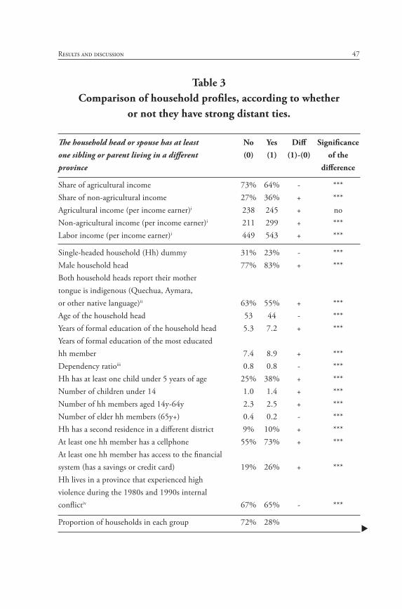
Table 3 compares the descriptive profile of households with strong distant ties with those without such ties. On average, the former group
47Results and discussion
Table 3Comparison of household profiles, according to whether
or not they have strong distant ties.
The household head or spouse has at least No Yes Diff Significanceone sibling or parent living in a different (0) (1) (1)-(0) of theprovince difference
Share of agricultural income 73% 64% - ***Share of non-agricultural income 27% 36% + ***Agricultural income (per income earner)i 238 245 + noNon-agricultural income (per income earner)i 211 299 + ***Labor income (per income earner)i 449 543 + ***
Single-headed household (Hh) dummy 31% 23% - ***Male household head 77% 83% + ***Both household heads report their mothertongue is indigenous (Quechua, Aymara,or other native language)ii 63% 55% + ***Age of the household head 53 44 - ***Years of formal education of the household head 5.3 7.2 + ***Years of formal education of the most educatedhh member 7.4 8.9 + ***Dependency ratioiii 0.8 0.8 - ***Hh has at least one child under 5 years of age 25% 38% + ***Number of children under 14 1.0 1.4 + ***Number of hh members aged 14y-64y 2.3 2.5 + ***Number of elder hh members (65y+) 0.4 0.2 - ***Hh has a second residence in a different district 9% 10% + ***At least one hh member has a cellphone 55% 73% + ***At least one hh member has access to the financialsystem (has a savings or credit card) 19% 26% + ***Hh lives in a province that experienced highviolence during the 1980s and 1990s internalconflictiv 67% 65% - ***
Proportion of households in each group 72% 28%

48 Revisiting the determinants of non-farm income in the Peruvian Andes
reports a higher labor income and diversifies more into non-agricul-tural activities than the latter.21 The second panel of Table 3, in turn, shows that these differences in economic outcomes are not necessarily due to the ties but—at least partially—to other characteristics as well.
Households with strong distant ties are on average younger (al-though the ratio of dependency, usually associated with economic vulnerability, is similar), more educated, and slightly less likely to be indigenous. A higher proportion of these households reports ac-cess to communication technologies (cellphones) and financial ser-vices. The household’s access to financial services refers to owning a debit or a credit card, something that may be associated with being a
21 As previously mentioned, although the information provided about labor income by the 2014 EPHR is consistent with official data on poverty and income for the Andean region (Enaho 2014), the information about non-labor income is not. This increases the need to control for other characteristics of the household and the environmental conditions that surround it (climate, economy, political violence background) that may account for non-labor income differences between households.
i Real income was spatially deflated using the poverty line (Enaho 2014).ii Households report on the first language the head or spouse (if there is one) learned to
speak as a child: 39% of households report that both have Spanish as their mother tongue, 58% of households report that both have an indigenous mother tongue, and only 3% of households report that one has an indigenous language and the other Spanish as a mother tongue.
iii Ratio of dependent to independent household members: number of children [<14y] and seniors [65y+] per income earner [14y-64y]).
iv Classification by Ponce (2010: 81-82) based on information gathered by the Truth and Reconciliation Commission (2003) for the period 1980-2000.
Note: According to the 2014 EPHR, 52% of rural households have strong ties in a differ-ent province, when they include siblings, parents, and/or children of the household head or spouse. The statistics are adjusted by the sampling design (weights, stratification, and clustering).

49Results and discussion
beneficiary of public transfer programs like Juntos (conditional cash transfer program) or Pension 65 (for the elderly population living in extreme poverty).
Beyond individual characteristics, a substantial proportion of rural households in the Andean region were strongly affected by the internal conflict in the eighties and nineties. Although two decades have passed, it is reasonable to expect that the consequences of the in-ternal conflict linger and still affect the social and economic dynamics in provinces that suffered high rates of violence during the war. The medium- and long-term consequences of the internal conflict in such provinces may range from different degrees and patterns of internal migration (emigration in war times and eventual return migration when peace was achieved) and the separation of families and weaken-ing of local family ties, to more institutional issues such as the under-mining of trust and social organizations.
Based on census information and the report by the Truth and Reconciliation Commission (CVR 2003), Ponce (2010: 17) shows that population growth between 1981 and 2005 was lower in prov-inces highly affected by violence during the internal conflict. While the population in provinces with low rates of violence grew by 45%, population in provinces with high rates grew only 30% between 1981 and 2005.22 The difference is mainly driven by the inter-census period 1981-1993, when the conflict was at its peak (the population grew 22% and 12% in low and high violence provinces, respectively).
Ponce (2010: 39) shows a much higher internal migration rate within provinces with high rates of violence during the internal conflict
22 Since the 1981 population census is not available for the regions of Loreto, San Martin, and Apurimac, the calculations involving population growth did not include these regions (Ponce 2010: 17). However, the classification used in the present study does include the Andean provinces in Apurimac (San Martin and Loreto are included in the EPHR only as Amazon regions).

50 Revisiting the determinants of non-farm income in the Peruvian Andes
as compared to provinces with low violence. The rate of internal migra-tion, defined in that study as the proportion of individuals that were born in a rural province but lived in a different province in the census year, rose from 26% in 1981 to 55% in 1993 in high violence prov-inces, whereas it decreased from 65% to 55% in the same period in low violence provinces. During the following period (1993-2007), however, internal migration rates are very similar (46% vs 50% in high and low violence, respectively).
Although the objective of this study is not to analyze the influ-ence of the provinces’ historical backgrounds on their socio-economic dynamics, it is clear that the historical background related to violence during the internal war should be considered when analyzing the ef-fect of strong distant ties and even climate change on strategies of income diversification. Table 3 shows that the prevalence of rural households living in provinces that experienced high violence is simi-lar between the group with strong distant ties and the group with no such ties (65% and 67%, respectively). The estimation in the next section controls for this background factor.
Finally, some caveats are worth mentioning. The connections I analyze here exclude strong ties living out of the country. Given that most rural households in the sample live in precarious conditions, I do not expect that such connections would substantially impact the households’ labor income diversification strategies (providing export/import business opportunities, for instance).23 However, remittances from international migrants may affect the investment resources that rural households may use for their self-employment activities, both on-farm and off-farm. The analysis also excludes temporarily absent strong ties, perhaps due to seasonal migration, which may correlate
23 Even though I do expect effects on households’ non-labor income and decisions to migra-te, I expect a negligible effect on short-term labor income decisions.
51Results and discussion
with households’ access to off-farm employment opportunities. Such ties are not distant but local, and I expect them to have effects similar to what Granovetter and others predict: the information is already known by the rural household (and its closest network), and entails no significant opportunities. It is also important to note that I have no information on which household has migrated, whether it is the rural household surveyed or the relatives that it reports as distant ties.
2. Estimation results
In this section I discuss the results of the estimation of the determi-nants of rural households’ diversification into non-farm activities. The two outcomes of interest are the share of non-farm labor income and the proportion of working hours allocated to non-farm activities. As previously mentioned, non-farm labor includes non-farm wage and self-employment. These estimates inform about the effects of intrasea-sonal climate variability and strong distant ties on non-farm income and hour shares for all rural Andean households, including farmers and non-farmers. The estimates of climate variability more clearly in-form about the sectorial effects, given that all agricultural activities are excluded from the non-farm sector.
The effects of intraseasonal climate variability on household in-come diversification strategies
Controlling for household characteristics and environmental condi-tions (discussed in detail in the next subsection), the estimates for the Andean region confirm the hypothesis that an increase in intraseasonal

52 Revisiting the determinants of non-farm income in the Peruvian Andes
climate variability leads to an increase in the relative importance of non-farm income and working hours in the household’s diversification strategy. When allowing for domain heterogeneity, I find similar results in the Central and Northern areas.
In the Southern domain, however, we find different results. While the effects of intraseasonal climate variability on the shares of non-farm income and working hours are statistically insignificant, we find puzzling results in the agricultural working hours and non-farm income level regressions. On the one hand, an increase in climate vari-ability increases the number of working hours allocated to agricultural activities, with no effects on the associated income levels. This could be consistent with this being an area of households that are more de-pendent on the agricultural activity (i.e., with less access to non-farm alternatives) that work longer hours on the farm to tend to their crops and pastures and deal with the effects of higher climate variability, with no higher income associated. The result on non-farm income (negative effect), on the other hand, suggests that higher intraseasonal climate variability induces households to reduce the allocation of re-
Table 4Summary of Tobit estimates of the effect of intraseasonal climate
variability on household income diversification strategies, in shares (Tables VIII.2 and VIII.3 in the Appendix).
Domain in the Andean Share of working hours Share of labor income obtainedregion allocated to non-farm activities from non-farm activities
All domains + *** + ***Northern + ** + **Central + ** + ***Southern - -
*** p<0.01, ** p<0.05, * p<0.1

53Results and discussion
sources (other than labor) to non-farm activities in favor of farm ac-tivities, thus reducing non-farm income levels.
The climatic variables show different variability and correla-tion across domains—Northern, Central, and Southern (see Appen-dix VIII.11). Regarding econometric specifications, Dell, Jones, and Olken (2014: 742), quoting Auffhammer et al. (2013), mention that “temperature and precipitation tend to be correlated, with a sign that varies by region. Thus, failing to include both could lead to omit-ted variables bias when interpreting a particular climatic variable es-timated in isolation.” Accordingly, the estimation models included the three climatic indicators (temperature range, average temperature, and precipitation). In order to explore the differences in variability and correlation across domains, we estimated an aggregate version for the Andean region and three separate versions for each domain.24 Each model includes an interaction term between temperature range
Table 5Summary of Tobit estimates of the effect of intraseasonal climate variability on household income diversification strategies, in levels
(Tables VIII.4, VIII.5, VIII.6 and VIII.7 in the Appendix)
Domain in the Hours of work in Non-farm Hours of work in AgriculturalAndean region non-farm activities income agricultural activities income
All domains + *** + *** - *** - ***Northern + ** + * - *** - ***Central + *** + * - *** - ***Southern - - ** + *** +
*** p<0.01, ** p<0.05, * p<0.1
24 Due to collinearity issues, we could not include the interaction between domain dummies and climate variables in the aggregate version.

54 Revisiting the determinants of non-farm income in the Peruvian Andes
and average temperature, to explore the hypothesis that farm income and hours in colder areas are relatively more affected by intraseasonal climate variability than in warmer areas.
Figure 2 shows the effects of intraseasonal climate variability for different temperature levels, under the regressions estimated by do-main.25 As previously mentioned, the average results for the North-ern and Central domains are consistent with this study’s hypothesis. Regarding the effect of intraseasonal climate variability across tem-peratures, however, only the Central domain shows the pattern we expected: a wider range of temperatures in the crop growing trimester can become a significant risk to crop survival in cold areas, which leads to a higher increase in non-farm income in colder areas. Two thirds of Andean households, and 70% of households in the Central Andes, live in districts with an average temperature below 13˚C dur-ing the November-January trimester (Appendix VIII.13).
The net effect of strong distant ties on household labor income
Following the conceptual framework and empirical specification dis-cussed in the previous section, I estimated the effect of strong distant ties on the degree of diversification outside of agricultural activities among rural Andean households. Besides information on households’ strong distant ties, I included two additional controls that may convey similar effects on household diversification strategies:
25 The noticeable differences between domains in Graph 2 makes evident the heterogeneity across domains. Appendix VIII.12 shows the graphs for the aggregate estimation (for all domains).
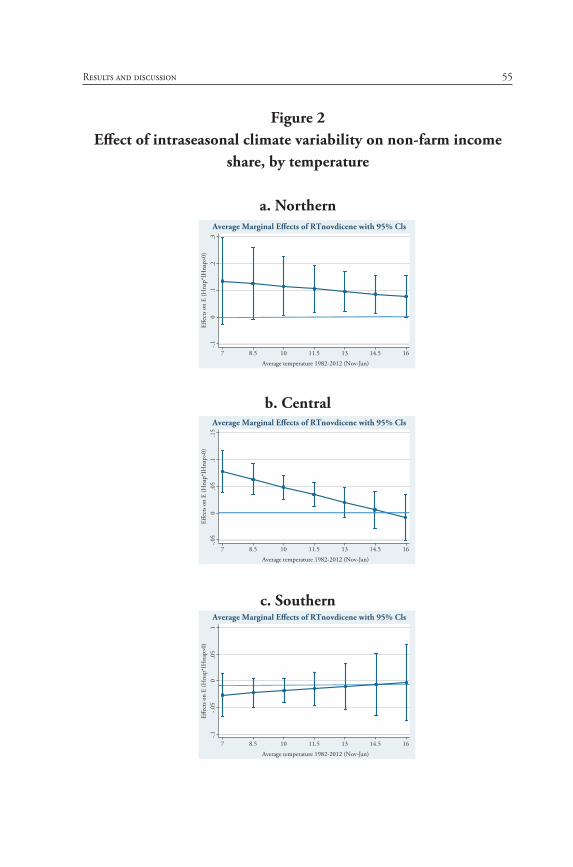
55Results and discussion
Average Marginal Effects of RTnovdicene with 95% Cls
7 8.5 10 11.5 13 14.5 16
Average temperature 1982-2012 (Nov-Jan)
.3.2
.10
-.1Eff
ects
on E
(Hna
p*IH
nap>
0)
Average Marginal Effects of RTnovdicene with 95% Cls
7 8.5 10 11.5 13 14.5 16
Average temperature 1982-2012 (Nov-Jan)
.15
.1.0
50
-.05
Effec
ts on
E (H
nap*
IHna
p>0)
Average Marginal Effects of RTnovdicene with 95% Cls
7 8.5 10 11.5 13 14.5 16
Average temperature 1982-2012 (Nov-Jan)
1.0
50
-.05
-.1Eff
ects
on E
(Hna
p*IH
nap>
0)
Figure 2Effect of intraseasonal climate variability on non-farm income
share, by temperature
a. Northern
b. Central
c. Southern

56 Revisiting the determinants of non-farm income in the Peruvian Andes
(i) Weak ties linking households with distant markets. As previously discussed, Granovetter and others have shown the importance of weak ties in economic outcomes, which need to be accounted for in order to isolate the effect of distant but strong ties. I control for the proportion of households in the district of residence that have strong distant ties (siblings or parents of the household head or spouse living permanently in a different province). Given that weak and strong ties may complement or substitute for one an-other, I include an interaction term as well. The estimates shown in the Appendix and Tables that follow represent marginal effects of each covariate. As new information becomes available, these es-timates should be complemented by other measures of strong and weak local ties, to give a more thorough picture of households’ networks and their role in income diversification strategies.
(ii) An additional dwelling used frequently by the household in a different town (in the same district or elsewhere). As mentioned before, a second dwelling (within or outside the district) allows the rural household to substantially reduce the costs involved in accessing other local or regional input, labor, or product markets.
Tables 6 and 7 summarize the estimates of the effect of strong distant family ties on household income diversification strategies (de-tailed results are included in the Appendix VIII.2-VIII.7). Four ver-sions of each model were estimated in order to account for potential regional heterogeneities: one for the rural Andean region, and one for each domain (Northern, Central, and Southern). As Table 6 shows, strong distant ties play a significant role in income diversification strategies, increasing the relative importance of non-farm activities. According to the estimates, both the share of non-farm working hours and non-farm income increase with strong distant ties in all domains, although the Northern area estimates are not statistically significant.

57Results and discussion
Table 6Summary of Tobit estimates of the effects of strong distant ties
on income diversification strategies, in shares (Tables VIII.2 and VIII.3 in the Appendix)
Domain in the Andean Share of working hours Share of labor income obtainedregion allocated to non-farm activities from non-farm activities
All domains + *** + ***Northern + +Central + * + *Southern + * + *
*** p<0.01, ** p<0.05, * p<0.1
Where does this effect of a higher importance of non-farm activi-ties come from? The effect is channeled through an increase in non-agricultural hours and income levels (rather than a negative impact on agricultural activities). As Table 7 shows, the effect of strong distant ties is positive and significant on non-agricultural income levels as well as on the number of hours allocated to this economic sector. Agricultural activities, however, are not significantly affected by these types of networks.26
Following the previous discussion, this finding is consistent with the idea that strong distant ties bring new information and oppor-tunities to the household, information that would otherwise not be available through local networks. The new information and oppor-tunities could include information about production technologies, access to more profitable markets (either new markets or the same
26 Interestingly, the Northern and Central domains show a positive effect on income and a decrease in hours. This would suggest that a lower allocation of work yields higher income (increase in labor productivity) when the household has strong distant ties. However, this result is not statistically significant.

58 Revisiting the determinants of non-farm income in the Peruvian Andes
markets at a lower cost), new employment opportunities (perhaps sea-sonal), among others.
Table 7Summary of Tobit estimates of the effects of strong distant ties
on income diversification strategies, in levels(Tables VIII.4, VIII.5, VIII.6 and VIII.7 in the Appendix)
Domain in the Hours of work in Non-farm Hours of work in AgriculturalAndean region non-farm activities income agricultural activities income
All domains + *** + *** - -Northern + ** + ** - +Central + ** + ** - +Southern + ** + ** - -
*** p<0.01, ** p<0.05, * p<0.1
Several controls are included in these estimations. Although these are not the focus of the study, it is interesting to note that most of the estimated parameters show the expected signs. More importantly, in most cases, the sign and significance of these parameters confirm the relevance of including them as controls in each estimation.
The findings on the role of demographic characteristics and edu-cation are consistent with the findings on non-agricultural income documented in the literature (Laszlo 2008, Escobal 2001, Reardon et al. 2001, among others). In most cases, results are similar for both versions of the models of working hours share and levels as well as for the models of income share and levels.
Regarding household demographics, it is important to mention that 66% of single-headed households are led by a woman, and 90% of female-headed households are single-headed. Thus, the vulner-ability that being single-headed entails is very much related to the

59Results and discussion
vulnerabilities that female-headed households face. In the Andean region, male households tend to have more access to land and other resources (especially in highland communities where traditional insti-tutions control access to land and water), and thus it is not surpris-ing that being a single-headed household is found to be associated with having a higher non-agricultural income share and level, ceteris paribus. The age of the household head is also a significant factor in the decision about income diversification strategies, not only because younger household heads are less likely to access land controlled by communities, but also because of the skills required to venture into non-agricultural activities.
As expected, education is a key factor in the decision about liveli-hood strategies. Given that rural household members have a key role in the decisions about income-generating strategies (as opposed to the traditional idea that households depend mainly on the household head), I control for the maximum level of education achieved by any of the household members. Even if the household head or spouse has no formal higher education, their children may provide the skills needed to embark on more profitable activities (either agricultural or non-agricultural).
Finally, the number of household members and the dependen-cy ratio capture the role of the demographic structure of the family. While more household members can mean a larger labor force and additional skills to contribute to the family livelihood, having too many children or elder members relative to economically active mem-bers can be burdensome for the household and limit its possibilities for engaging in profitable economic activities, especially when they require working outside of the farm. The estimation results in Appen-dices VIII.4-VIII.7 show that, controlling for the dependency ratio, the number of family members does positively affect the income levels

60 Revisiting the determinants of non-farm income in the Peruvian Andes
that households generate from each activity, as well as the number of hours allocated to either farm or non-farm activities. Other assets such as land size, access to financial services, and a second dwelling (nearby, in the same district in most cases) show the expected signs. Whereas an increase in land size is associated with higher agricultural income, access to financial services and owning a second dwelling fa-vors non-agricultural activities.
Besides household characteristics and assets, the estimation con-trols for local conditions, some of them directly related to the house-hold’s economic activities, and others seeming to indirectly affect out-comes through their effects on market and social institutions.
In order to control for market dynamics, I introduced three indi-cators. For the agricultural sector I controlled for farmers’ connection to agricultural markets (proxied by the proportion of farmers in the province that sell most of the yield produced in one or more plots in the market) and the province’s agricultural labor productivity (prox-ied by the median hourly agricultural earnings in the province). As Appendix VIII.6 and VIII.7 show, an increase in the province’s agri-cultural labor productivity increases the incentive to work in the agri-cultural sector, thus increasing both working hours allocated to farm activities (wage and self-employment) and the derived agricultural income, and decreasing non-farm hours and income. Interestingly, an increase in the province’s non-farm labor productivity increases a household’s agricultural income but has no effect on the hours allo-cated to farm activities, which suggests an increase in the household’s agricultural productivity (and cross-sector spillover effects).
At the same time, an increase in the province’s non-farm produc-tivity reduces the number and share of hours allocated to non-agri-cultural activities, but interestingly, this has no effect on the associ-ated income levels or share. This would suggest an improvement in

61Results and discussion
households’ non-agricultural labor productivity based on the province’s increase in non-agricultural productivity. However, I call for a cautious interpretation of this parameter, given that the non-agricultural sector in rural economies is highly heterogeneous. This high heterogeneity is noticeable in the contrast between the average non-agricultural share of rural labor income, 50% (Graph 1), and the average household non-farm income shares, 29% (Appendix VIII.8).
As expected, improved access to public services induces an in-crease in non-agricultural income levels and share. However, the ef-fect on agricultural levels is negative, which may seem a bit puzzling. Based on the results in the hours model, I argue that the effect on income may be induced by the reduced number of hours allocated to agriculture, instead of a counterintuitive reduction in productivity or increase in transaction costs that discourages access to more profit-able markets. I also introduced a control for a historical background of violence during the internal conflict and the associated economic disruption and social and political instability (Ponce 2010, based on information from the CVR 2003). The estimates in Appendix VIII.2 and VIII.3 show that, ceteris paribus, moving from a province with no history of severe violence to one that experienced high violence would induce a change in diversification strategies in favor of agricultural activities.


5. CONCLUSIONS AND FINAL REMARKS
Previous studies have documented transformations in the Peruvian Andes, ranging from the increasing share of non-farm (i.e., non-ag-ricultural) activities in rural households’ livelihoods, to internal mi-gration and increasing connectivity between rural and urban areas, to changing climate conditions. Using cross-sectional information representative of provinces in the Andean region, as well as previous climate estimates for the region (Ponce, Arnillas, & Escobal 2015), this paper analyzes the role of distant, yet strong family networks (sib-lings and parents of the household head or spouse living in a different province) and intraseasonal climate variability (30-year averages) on the household decisions to diversify into non-farm activities.
To estimate the role of strong distant ties and intraseasonal cli-mate variability in the relative importance of non-farm activities and household labor income, two economic outcomes were analyzed: the share of non-farm working hours and the share of non-farm labor income. The estimations of the effect of each of the two variables on both outcomes controlled for household demographics and assets as well as economic characteristics, such as provincial proxies for labor productivity in the agricultural and non-agricultural sectors. Institu-tional and historical features were also included in the estimation, proxied by the degree of inequality in the distribution of agricultural land (affecting access to key assets), and dummies for provinces that suffered from severe violence during the internal war in the eighties

64 Revisiting the determinants of non-farm income in the Peruvian Andes
and nineties (which, some argue, has had lingering effects on socio-economic and micro-political conditions). Finally, the estimations controlled for other climate conditions such as 30-year averages of temperature and precipitation, the change in these conditions over the last 20 years, and the prevalence of irrigation systems in districts, to account for other key environmental conditions for agricultural activities.
Controlling for other assets and environmental conditions, we find that households with strong distant ties tend to diversify more into non-farm activities. This effect is smaller in areas where other households also have such distant ties (a proxy for weak ties). This suggests a substitution effect between strong distant ties and weak ties. Complementarily, having a second residence in a different town also increases non-farm income shares. These results are consistent with the hypothesis that strong distant ties are key assets for accessing (or reducing costs of access to) new markets or new information relevant to income-generating activities. These results suggest that interven-tions aimed at increasing economic opportunities for rural house-holds should include information and communication technologies and other resources that enhance their ability to capitalize on the as-sets of distant networks.
As for the effects of intraseasonal climate variability, the results show that increases in climate variability (proxied by the temperature range during the November-January crop growing trimester) lead to an overall increase in the relative importance of non-farm activities in both household income and household working hours. However, when analyzed separately by domain, the results remain only for the Northern and Central domains; the Southern domain shows no sig-nificant effect. The results for the Central Andean region show that this positive impact is stronger in colder areas, and significant below 13˚C.

65Conclusions and final remarks
Since two thirds of Andean households, including 70% of households in the Central Andes, live in districts with an average temperature be-low 13˚C during the November-January trimester, the result is robust for a large sector of the Andean region.
These results suggest that interventions focused on helping farm-ers cope with climate change should consider not only farm activities but also the skills and assets required for accessing off-farm activities. A household’s distant (non-local) networks is a type of asset that is usually neglected in development projects, but according to our re-sults, it can play a role in improving household income.


REFERENCES
Berdegué, Julio; Anthony Bebbington, and Javier Escobal (2015). Conceptualizing spatial diversity in Latin American rural develop-ment: structures, institutions, and coalitions. World Development, 73, 1-10, http://dx.doi.org/10.1016/j.worlddev.2014.10.015.
Berdegué, Julio, and Felix Modrego Benito (2012). De Yucatán a Chi-loé: dinámicas territoriales en América Latina. Buenos Aires: IDRC, RIMISP and Editorial Teseo.
Caballero, José María, and Elena Alvarez (1980). Aspectos cuantitativos de la reforma agraria 1969-1979. Lima: IEP.
Comisión de la Verdad y Reconciliación (2003). Informe final - VIII tomos. Lima. Retrieved from http://www.cverdad.org.pe/ifinal/index.php.
Claverías, Ricardo (2000). Conocimientos de los campesinos andinos so-bre los predictors climáticos: elementos para su verificación. CIED. Retrieved from http://clima.missouri.edu/Articles/Claverias_Bio-indicadores.pdf
Damonte, Gerardo (2011). Construyendo territorios: narrativas territo-riales aymaras contemporáneas. Lima: GRADE and CLACSO.
Dasgupta, Purnamita; John F. Morton, David Dodman, Baris Kara-pinar, Francisco Meza, Marta G. Rivera-Ferre, Aisa Toure Sarr, and Katharine E. Vincent (2014). Rural areas. In Christopher B.
68 Revisiting the determinants of non-farm income in the Peruvian Andes
Field, Vicente R. Barros, David J. Dokken, Katharine J. Mach, Michael D. Mastrandrea, T. Eren Bilir, Monalisa Chatterjee, Kris-tie L. Ebi, Yuka O. Estrada, Robert C. Genova, Betelhem Girma, Eric S. Kissel, Andrew N. Levy, Sandy MacCracken, Patricia R. Mastrandrea, and Leslie L. White (Eds.), Climate change 2014: impacts, adaptation, and vulnerability. Part A: global and sectoral aspects. Contribution of Working Group II to the Fifth Assessment Report of the Intergovernmental Panel on Climate Change (pp. 613-657). Cambridge: Cambridge University Press.
Dell, Melissa; Benjamin F. Jones, and Benjamin A. Olken (2014). What do we learn from the weather?: the new climate-economy literature. Journal of Economic Literature, 52(3), 740-798. DOI: 10.1257/jel.52.3.740
Dirven, Martini (2004). Rural non-farm employment and rural diver-sity in Latin America. CEPAL Review, 83, 47-66.
Earls, John (1991). Organización económica y tecnología en la cultura andina. In Ecologia y agronomia en los Andes. Alternativas étnicas al desarrollo. La Paz: Hisbol.
Escobal, Javier (2001). The determinants of non-farm income diversi-fication in rural Peru. World Development, 29(3), 497-508.
Escobal, Javier, and Carmen Ponce (2010). Adaptación al cambio cli-mático en contextos de desarrollo territorial rural: la experiencia de Jauja. In Cambio climático en la cuenca del rio Mantaro: balance de siete años de estudios (pp. 226-233). Lima: Instituto Geofísico del Perú.
Escobal, Javier, and Carmen Ponce (2012). Una mirada de largo plazo a la economía campesina en los Andes. In Desarrollo rural y recur-sos naturales (pp. 15-93). Lima: GRADE.

69References
Figueroa, Adolfo (1989). La economia campesina de la sierra del Peru (Fourth edition). Lima: PUCP.
Giulietti, Corrado; Jackline Wahba, and Yves Zenou (2014). Strong versus weak ties in migration. IZA Discussion Papers, 8089. Insti-tute for the Study of Labor (IZA).
Glave, Manuel, and Karla Vergara (2016). Cambio global, alta mon-taña y adaptación: una aproximación social y geográfica. In Inves-tigación para el desarrollo en el Peru: once balances (pp. 445-507). Lima: GRADE.
Grammont, Hubert C. de (2008). El concepto de nueva ruralidad. In Edelmira Pérez, María Adelaida Farah and Hubert C. de Gram-mont (Comp.), La nueva ruralidad en América Latina: avances teó-ricos y evidencias empiricas (pp. 23-44). Lima: Editorial Pontificia Universidad Javeriana and CLACSO.
Granovetter, Mark (1985). Economic action and social structure: the problem of embeddedness. American Journal of Sociology, 91(3), 481-510.
Granovetter, Mark (2005). The impact of social structure on economic outcomes. Journal of Economic Perspectives, 19(1), 33-50.
Golte, Jurgen (1980). La racionalidad de la organización andina. Lima: IEP.
Hazell, Peter; Steven Haggblade, and Thomas Reardon (2007). Struc-tural transformation of the rural nonfarm economy. In Steven Haggblade, Peter Hazell, and Thomas Reardon, Transforming the rural non-farm economy: opportunities and threats in the develo-ping world (pp. 83-98). Baltimore, MD: John Hopkins Univer-sity Press

70 Revisiting the determinants of non-farm income in the Peruvian Andes
Hernández Asensio, Raúl (2012). Nuevas (y viejas) historias sobre las mu-jeres rurales jóvenes de América Latina: resultados preliminares del Pro-grama Nuevas Trenzas. Serie Programa Nuevas Trenzas, 1. Lima: IEP. Retrieved from http://bibliotk.iep.org.pe/bib_img/36966-8-1.pdf
Hicks, Joan Hamory; Marieke Kleemans, Nicholas Y. Li, and Edward Miguel (2017). Reevaluating agricultural productivity gaps with longitudinal microdata. NBER Working Paper 23253. Retrieved from http://www.nber.org/papers/w23253.pdf
Himanshu, H.; Peter Lanjouw, Rinku Murgai, and Nicholas Stern (2013). Non-farm diversification, poverty, economic mobility, and income inequality: a case study in village India. Agricultural Economics, 44(4-5), 461-473.
IGP (2005). Atlas climático de precipitación y temperatura del aire de la Cuenca del Rio Mantaro. Lima: Consejo Nacional del Ambiente (CONAM) and Instituto Geofísico del Perú (IGP).
IGP (2005). Diagnóstico de la Cuenca del Mantaro bajo la visión del cambio climático. Lima: Consejo Nacional del Ambiente (CO-NAM) and Instituto Geofísico del Perú (IGP).
IGP (2005). Vulnerabilidad actual y futura ante el cambio climático y medidas de adaptación en la Cuenca del Rio Mantaro. Lima: Con-sejo Nacional del Ambiente (CONAM) and Instituto Geofísico del Perú (IGP).
INEI (2009). Migraciones internas 1993-2007. Lima. Retrieved from https://www.inei.gob.pe/media/MenuRecursivo/publicaciones_digitales/Est/Lib0801/libro.pdf
INEI (2017). Evolución de la pobreza monetaria 2007-2016. Informe Técnico. Retrieved from https://www.inei.gob.pe/media/cifras_de_pobreza/pobreza2016.pdf
71References
Ioannides, Yannis and Linda Datcher Loury (2004). Job information networks, neighborhood effects, and inequality. Journal of Econo-mic Literature, 42(4), 1056-93.
IPCC (2014a). Climate change 2014: impacts, adaptation, and vulne-rability. Summaries, frequently asked questions, and cross-chapter boxes. A Working Group II Contribution to the Fifth Assessment Report of the Intergovernmental Panel on Climate Change. In Christopher B. Field, Vicente R. Barros, David Jon Dokken, Ka-tharine J. Mach, Michael D. Mastrandrea, T. Eren Bilir, Monalisa Chatterjee, Kristie L. Ebi, Yuka O. Estrada, Robert C. Genova, Betelhem Girma, Eric S. Kissel, Andrew N. Levy, Sandy Mac-Cracken, Patricia R. Mastrandrea, and Leslie L. White (Eds.) Fif-th assessment report of the intergovernmental panel on climate chan-ge. Geneva, Switzerland: World Meteorological Organization. Retrieved from https://www.ipcc.ch/pdf/assessment-report/ar5/wg2/WGIIAR5-IntegrationBrochure_FINAL.pdf
IPCC (2014b). Annex II: glossary [Katharine J. Mach, Serge Planton and Christoph von Stechow (Eds.)]. In Core Writing Team, Ra-jendra K. Pachauri, and Leo Meyer (Eds.), Climate change 2014: synthesis Report. Contribution of Working Groups I, II and III to the Fifth Assessment Report of the Intergovernmental Panel on Clima-te Change (pp. 117-130). Geneva, Switzerland: IPCC. Retrieved from https://www.ipcc.ch/pdf/assessment-report/ar5/syr/AR5_SYR_FINAL_Annexes.pdf
Jackson, Matthew; Brian Rogers, and Yves Zenou (2017). The econo-mic consequences of social-network structure. Journal of Econo-mic Literature, 55(1), 1-47.
Lanjouw, Peter (2007). Does the rural non-farm economy contribute to poverty reduction? In Steven Haggblade, Peter B.R. Hazell,

72 Revisiting the determinants of non-farm income in the Peruvian Andes
and Thomas Reardon, Transforming the rural non-farm economy (pp. 55-79). Baltimore, MD: John Hopkins University Press.
Lanjouw, Peter, and Rinku Murgai (2009). Poverty decline, agricultu-ral wages, and non-farm employment in rural India: 1983–2004. Agricultural Economics, 40(2), 243–263.
Laszlo, Sonia (2008). Education, Labor supply, and market develop-ment in rural Peru. World Development, 36(11), 2421-2439.
Lavado, Waldo; Grinia Ávalos, and Wouter Buytaert (2015). La eco-nomia del cambio climático en el Peru: la climatologia del cambio climático. Monografía, 262 (MG-262). Washington, DC: Banco Interamericano de Desarrollo.
Lin, Brenda (2011). Resilience in agriculture through crop diversifica-tion: adaptive management for environmental change. BioScience, 61(3), 183-193.
Llona, Marianna; Daniel Ramirez, and Mario Zolezzi (2004). Las ciu-dades intermedias: su rol en el desarrollo del pais. Peru Hoy, 6. Lima: DESCO. Retrieved from http://urbano.org.pe/descargas/investi-gaciones/PERU-HOY/PH-2004.PDF
Magrin, Graciela O.; José A. Marengo, Jean Phillipe Boulanger, Mar-cos S. Buckeridge, Edwin Castellanos, Germán Poveda, Fabio R. Scarano, and Sebastián Vicuña (2014). Central and South America. In Vicente R. Barros, Christopher B. Field, David Jon Dokken, Michael D. Mastrandrea, Katharine J. Mach, T.E. Bilir, Monalisa Chatterjee, Kristie L. Ebi, Yuka O. Estrada, Robert C. Genova, Betelhem Girma, Eric S. Kissel, Andrew N. Levy, Sandy MacCracken, Patricia R. Mastrandrea, and Leslie L. White (Eds.), Climate Change 2014: impacts, adaptation, and vulnerability. Part B: regional aspects. Contribution of Working Group II to the Fifth

73References
Assessment Report of the Intergovernmental Panel on Climate Chan-ge (pp. 1499-1566). Cambridge: Cambridge University Press. Re-trieved from http://www.ipcc.ch/pdf/assessment-report/ar5/wg2/WGIIAR5-Chap27_FINAL.pdf
Mayer, Enrique (1979). Land use in the Andes: ecology and agricul-ture in the Mantaro Valley of Peru with special reference to pota-toes. Lima: CIP.
Mertz, Ole; Cheikh Mbow, Anette Reenberg, Lorenzo Genesio, Eric F. Lambin, Sarah D’haen, Malicki Zorom, Kjeld Rasmussen, Drissa Diallo, Bruno Barbier, Ibrahim Bouzou Moussa, Awa Diouf, Jo-nas Ø. Nielsen, and Inge Sandholt (2011). Adaptation strategies and climate vulnerability in the Sudano-Sahelian region of West Africa. Atmospheric Science Letters, 12(1), 104-108.
MINAM. Dirección General de Ordenamiento Territorial. Retrieved from http://www.minam.gob.pe/ordenamientoterritorial/que-es-el-ordenamiento-territorial/
Ponce, Carmen (2010). Pobreza y demografía: una visión de media-no plazo. Economia y Sociedad, 78, 24-30 Retrieved from http://www2.congreso.gob.pe/sicr/cendocbib/con4_uibd.nsf/5B05A94EC83C860B05257E0A007884A9/$FILE/03-ponce.pdf
Ponce, Carmen; Carlos Alberto Arnillas, and Javier Escobal (2015). Cambio climático, uso de riego y estrategias de diversificación de cultivos en la sierra Peruana. In Javier Escobal, Ricardo Fort y Eduardo Zegarra (Eds.), Agricultura peruana: nuevas miradas desde el censo agropecuario (pp. 171-223). Lima: GRADE.
Postigo, Julio (2012). Responses of plants, pastoralists, and governments to social environmental changes in the Peruvian Southern Andes (PhD Thesis). University of Texas, Austin.

74 Revisiting the determinants of non-farm income in the Peruvian Andes
Postigo, Julio, and Kenneth Young (Eds.) (2016). Naturaleza y so-ciedad: perspectivas socio-ecológicas sobre cambios globales en América Latina. Lima: Desco, IEP, and INTE-PUCP.
Reardon, Thomas; Julio Berdegué, and Germán Escobar (2001). Rural non-farm employment and incomes in Latin America: overview and policy implications. World Development, 29(3), 395-409. Re-trieved from https://doi.org/10.1016/S0305-750X(00)00112-1
Reardon, Thomas; Julio Berdegué, Christopher B. Barrett, and Kostas Stamoulis (2007). Household income diversification into rural nonfarm activities. In Steven Haggblade, Peter B.R. Hazell, and Thomas Reardon (Eds.), Transforming the rural nonfarm economy (pp. 115-140). Baltimore, MD: John Hopkins University Press.
Schetjman, Alexander, and Julio Berdegué (2004). Desarrollo territorial rural. Debates y Temas Rurales, 1. Santiago: RIMISP.
Senamhi (2007). Escenarios de cambio climático en la Cuenca del rio Mantaro para el año 2100. Lima.
Sobel, Joel (2002). Can we trust social capital? Journal of Economic Literature, 40(1), 139-154.
Valdivia, Corinne; Anji Seth, Jere L. Gilles, Magali García, Eliza-beth Jiménez, Jorge Cusicanqui, Fredy Navia, and Edwin Yu-cra (2010). Adapting to climate change in Andean ecosystems: landscapes, capitals, and perceptions shaping rural liveliho-od strategies and linking knowledge systems. Annals of the As-sociation of American Geographers, 100(4), 818-834. DOI: 10.1080/00045608.2010.500198
Vergara, Karla (2012). Variabilidad climática, percepción ambiental y estrategias de adaptación de la comunidad campesina de Con-chucos, Ancash (Thesis). Pontificia Universidad Católica del Perú;

75References
Lima. Retrieved from http://tesis.pucp.edu.pe/repositorio/han-dle/123456789/1240
Woolcock, Michael and Deepa Narayan (2000). Social capital: impli-cations for development theory, research, and policy. The World Bank Research Observer, 15(2), 225-249.
Young, Kenneth, and Jennifer Lipton (2006). Adaptive governance and climate change in the Tropical highlands of western South America. Climatic Change, 78(1), 63-102.
Zimmer, Anaïs, and Daniel Montes (2017). Territorio seguro y resilien-te. Caracteristicas y oportunidades del territorio en un contexto de cambio climático. Mancomunidad Municipal Waraq. Diagnóstico territorial, tendencia del clima y estrategias de adaptación al cam-bio climático. Lima: Instituto de Montaña and USAID. Retrieved from https://mountain.pe/wp-content/uploads/Territorio-segu-ro-y-resiliente-Mancomunidad-Municipal-Waraq.pdf
Data bases used in the study (www.inei.gob.pe):
EPHR 2014 - Provincial Survey of Rural Households.
Enaho 2014 - National Households Survey.
Cenagro 1994, 2012 – National Censuses.


APPENDIX
1. Internal migration between 1981 and 2005, by populations that were born in rural provinces (Table extracted from Ponce (2010: 39))
Percentage of rural population who emigrated from the province they were born to another province (years 1981, 1993 and 2007)
Note: This graph shows the proportion of individuals that were born in rural provinces but live in a different province with respect to all individuals born in rural provinces. The blue line represents provinces with high violence during the internal conflict, the red line represents the low violence provinces, and the yellow line combines all provinces. The table shows migration rates in the Coast, Andean, and Amazon regions altogether. Given that there is no 1981 census information available for Loreto, San Martin, and Apurimac, the calculations of this graph excluded individuals living in these 3 regions.Source: Ponce (2010: 39).
1981 1993Census year
2007
Total
70
60
50
40
30
20
10
0
Provinces with high violenceduring the internal conflict
Other provinces

78 Revisiting the determinants of non-farm income in the Peruvian Andes
2. Tobit model of the share of working hours allocated to non-farm activities
Household characteristics and All domains North Central Southenvironmental conditions
Single-headed household dummy 0.0636*** 0.0990*** 0.0650*** 0.0325** (0.00797) (0.0172) (0.0114) (0.0128)The mother tongue reported by -0.0695*** 0.128 -0.0757*** -0.107***household head and spouse is an (0.0121) (0.0854) (0.0148) (0.0245)indigenous language Age of the household head -0.00487*** -0.00337*** -0.00384*** -0.00698*** (0.000274) (0.000467) (0.000392) (0.000542)Dependency ratio (hh members -0.0273*** -0.0177* -0.0245*** -0.0368***[<14y,64y] / [14-64]) (0.00463) (0.00963) (0.00682) (0.00779)Years of formal education of the 0.0524*** 0.0481*** 0.0573*** 0.0457***most educated hh member (0.00138) (0.00291) (0.00210) (0.00200)Number of household members -0.00171 -0.00797** -0.00547** 0.00925*** (0.00196) (0.00379) (0.00266) (0.00344)Strong distant ties - the household 0.0222*** 0.0201 0.0186* 0.0247*has strong family ties in a different (0.00769) (0.0156) (0.0106) (0.0132)province (at least one sibling orparent of the household head orspouse) Weak ties (% of households in the 0.0496 0.0745 0.0125 0.310***district with strong distant ties) (0.0365) (0.0769) (0.0543) (0.0760)The household has a second 0.0585*** 0.0368 0.0546*** 0.0595***dwelling that it visits frequently (0.00999) (0.0253) (0.0143) (0.0154)Access to financial services 0.0604*** -0.00908 0.0806*** 0.122*** (0.00905) (0.0176) (0.0130) (0.0154)Land size (Owns) -2.08e-05*** -2.49e-05** -8.34e-06 -2.28e-05*** (5.35e-06) (1.11e-05) (7.40e-06) (8.25e-06)Unexpected climate events in the -0.0352 0.0392 -0.0915** 0.0812district (% of farmers in the district (0.0253) (0.0642) (0.0415) (0.0528)who had crops or pastures affectedby an unexpected climate eventduring the previous year)

79Appendix
Household characteristics and All domains North Central Southenvironmental conditions
30-year average temperature -0.00476 -0.000687 -0.00290 -0.00781(Nov/Dec/Jan) (0.00401) (0.00956) (0.00725) (0.00678)30-year temperature range 0.0305*** 0.0900** 0.0358*** -0.0160(Nov/Dec/Jan) (0.00778) (0.0370) (0.0112) (0.0122)30-year average precipitation 0.000598** 0.00179*** 0.000422 7.60e-05(Nov/Dec/Jan) (0.000274) (0.000546) (0.000479) (0.000480)Percentage of farmers with irrigation -0.0700*** -0.00835 -0.0912*** -0.0628systems (gravity or technified) in the (0.0226) (0.0739) (0.0346) (0.0434)district Land Gini coefficient (equivalent 0.452*** 0.696*** 0.453*** 0.0713hectares) (0.0620) (0.199) (0.0985) (0.116)Product market - Proportion of -0.0260 -0.308*** -0.0916** 0.251***farmers that allocate most yield (0.0275) (0.0647) (0.0390) (0.0580)from at least one plot to markets Non-agricultural sector - median -0.00331** -0.00981*** -0.00318 -0.00220hourly income in the province of (0.00137) (0.00325) (0.00203) (0.00279)residence Agricultural sector - median hourly -0.00561*** -0.00747 -0.00253 -0.0157***income in the province of residence (0.00149) (0.00508) (0.00211) (0.00274)% of households with access to safe 0.306*** 0.216*** 0.269*** 0.275***water (0.0281) (0.0814) (0.0384) (0.0645)The province experienced high -0.0335** -0.109*** 0.0110 -0.0754*violence during the internal conflict (0.0136) (0.0289) (0.0238) (0.0400)(1980’s, 1990’s)ii
Observations 63,275 12,062 29,349 21,864
Robust standard errors in parenthesis. *** p<0.01, ** p<0.05, * p<0.1ii Classification by Ponce (2010: 81-82) based on information gathered by the Truth and Recon-ciliation Commission (2003) for the period 1980-2000. Note: The estimates were adjusted by the sample design (stratified and clustered random sample).Source: own estimates based on data from the 2014 EPHR, 2012 Agricultural Census, identifica-tion of provinces that experienced high violence during the internal war by Ponce (2010), and climate estimates by Ponce, Arnillas, and Escobal (2015).

80 Revisiting the determinants of non-farm income in the Peruvian Andes
3. Tobit model of the share of labor income generated by non-farm activities
Household characteristics and All domains North Central Southenvironmental conditions
Single-headed household dummy 0.0601*** 0.0946*** 0.0618*** 0.0282** (0.00829) (0.0171) (0.0116) (0.0141)The mother tongue reported by -0.0679*** 0.135 -0.0717*** -0.108***household head and spouse is an (0.0126) (0.0915) (0.0150) (0.0256)indigenous language Age of the household head -0.00547*** -0.00364*** -0.00437*** -0.00800*** (0.000283) (0.000471) (0.000399) (0.000572)Dependency ratio (hh members -0.0276*** -0.0145 -0.0259*** -0.0386***[<14y,64y] / [14-64]) (0.00475) (0.00949) (0.00695) (0.00825)Years of formal education of the 0.0544*** 0.0476*** 0.0587*** 0.0494***most educated hh member (0.00131) (0.00270) (0.00191) (0.00200)Number of household members -0.00333* -0.0103*** -0.00725*** 0.00931** (0.00200) (0.00382) (0.00263) (0.00371)Strong distant ties - the household 0.0248*** 0.0250 0.0189* 0.0279*has strong family ties in a different (0.00800) (0.0156) (0.0108) (0.0144)province (at least one sibling orparent of the household head orspouse) Weak ties (% of households in the 0.0352 0.0624 0.00740 0.289***district with strong distant ties) (0.0376) (0.0766) (0.0545) (0.0805)The household has a second dwelling 0.0670*** 0.0523** 0.0513*** 0.0748***that it visits frequently (0.0104) (0.0253) (0.0144) (0.0169)Access to financial services 0.0652*** -0.0113 0.0866*** 0.148*** (0.00926) (0.0173) (0.0131) (0.0169)Land size (Owns) -2.34e-05*** -2.99e-05*** -9.48e-06 -2.35e-05*** (5.00e-06) (9.43e-06) (7.86e-06) (8.24e-06)Unexpected climate events in the -0.0287 0.0261 -0.0821** 0.0915district (% of farmers in the district (0.0260) (0.0667) (0.0415) (0.0568)who had crops or pastures affectedby an unexpected climate eventduring the previous year)
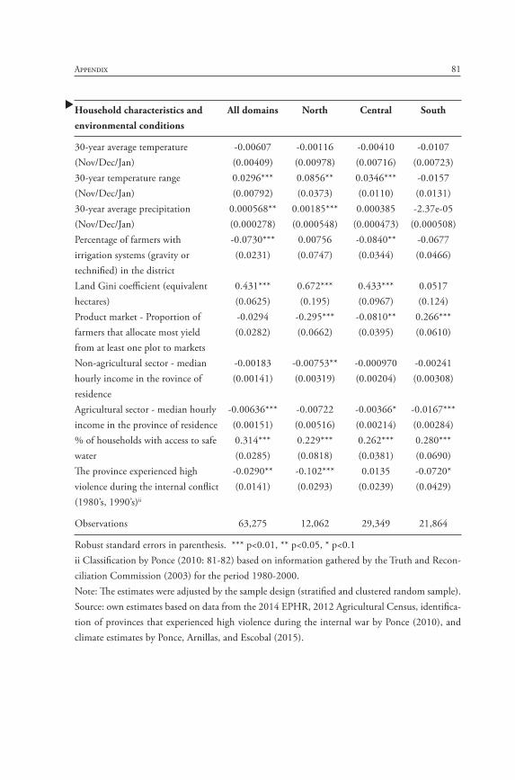
81Appendix
Household characteristics and All domains North Central Southenvironmental conditions
30-year average temperature -0.00607 -0.00116 -0.00410 -0.0107(Nov/Dec/Jan) (0.00409) (0.00978) (0.00716) (0.00723)30-year temperature range 0.0296*** 0.0856** 0.0346*** -0.0157(Nov/Dec/Jan) (0.00792) (0.0373) (0.0110) (0.0131)30-year average precipitation 0.000568** 0.00185*** 0.000385 -2.37e-05(Nov/Dec/Jan) (0.000278) (0.000548) (0.000473) (0.000508)Percentage of farmers with -0.0730*** 0.00756 -0.0840** -0.0677irrigation systems (gravity or (0.0231) (0.0747) (0.0344) (0.0466)technified) in the district Land Gini coefficient (equivalent 0.431*** 0.672*** 0.433*** 0.0517hectares) (0.0625) (0.195) (0.0967) (0.124)Product market - Proportion of -0.0294 -0.295*** -0.0810** 0.266***farmers that allocate most yield (0.0282) (0.0662) (0.0395) (0.0610)from at least one plot to marketsNon-agricultural sector - median -0.00183 -0.00753** -0.000970 -0.00241hourly income in the rovince of (0.00141) (0.00319) (0.00204) (0.00308)residence Agricultural sector - median hourly -0.00636*** -0.00722 -0.00366* -0.0167***income in the province of residence (0.00151) (0.00516) (0.00214) (0.00284)% of households with access to safe 0.314*** 0.229*** 0.262*** 0.280***water (0.0285) (0.0818) (0.0381) (0.0690)The province experienced high -0.0290** -0.102*** 0.0135 -0.0720*violence during the internal conflict (0.0141) (0.0293) (0.0239) (0.0429)(1980’s, 1990’s)ii
Observations 63,275 12,062 29,349 21,864
Robust standard errors in parenthesis. *** p<0.01, ** p<0.05, * p<0.1ii Classification by Ponce (2010: 81-82) based on information gathered by the Truth and Recon-ciliation Commission (2003) for the period 1980-2000. Note: The estimates were adjusted by the sample design (stratified and clustered random sample).Source: own estimates based on data from the 2014 EPHR, 2012 Agricultural Census, identifica-tion of provinces that experienced high violence during the internal war by Ponce (2010), and climate estimates by Ponce, Arnillas, and Escobal (2015).

82 Revisiting the determinants of non-farm income in the Peruvian Andes
4. Tobit model of the number of working hours allocated to non-farm activities
Household characteristics and All domains North Central Southenvironmental conditions
Single-headed household dummy 1.654*** 3.375*** 1.738*** 0.192 (0.361) (0.780) (0.506) (0.595)The mother tongue reported by -3.500*** 7.288 -3.319*** -4.900***household head and spouse is an (0.584) (4.682) (0.671) (1.165)indigenous language Age of the household head -0.147*** -0.0948*** -0.102*** -0.231*** (0.0113) (0.0221) (0.0163) (0.0196)Dependency ratio (hh members -3.545*** -3.059*** -3.358*** -3.996***[<14y,64y] / [14-64]) (0.229) (0.485) (0.320) (0.393)Years of formal education of the 2.441*** 2.207*** 2.577*** 2.248***most educated hh member (0.0550) (0.120) (0.0777) (0.0862)Number of household members 1.454*** 1.048*** 1.327*** 2.068*** (0.105) (0.232) (0.138) (0.170)Strong distant ties - the household 1.512*** 1.872** 1.111** 1.507**has strong family ties in a different (0.362) (0.754) (0.480) (0.630)province (at least one sibling orparent of the household head orspouse) Weak ties (% of households in the 1.474 3.504 -0.187 15.32***district with strong distant ties) (1.693) (3.649) (2.363) (3.575)The household has a second dwelling 3.365*** 2.603** 2.339*** 4.132***that it visits frequently (0.462) (1.195) (0.643) (0.720)Access to financial services 2.738*** -0.557 3.163*** 6.758*** (0.425) (0.845) (0.571) (0.735)Land size (Owns) -0.000953*** -0.00143*** -0.000163 -0.000973*** (0.000232) (0.000465) (0.000370) (0.000365)Unexpected climate events in the -0.373 3.266 -2.296 3.965district (% of farmers in the district (1.225) (3.251) (1.960) (2.632)who had crops or pastures affectedby an unexpected climate eventduring the previous year)

83Appendix
Household characteristics and All domains North Central Southenvironmental conditions
30-year average temperature -0.193 0.119 -0.106 -0.363(Nov/Dec/Jan) (0.186) (0.469) (0.326) (0.312)30-year temperature range 1.523*** 4.158** 1.603*** -0.601(Nov/Dec/Jan) (0.363) (1.700) (0.491) (0.605)30-year average precipitation 0.0255* 0.0978*** 0.0166 -0.00839(Nov/Dec/Jan) (0.0132) (0.0270) (0.0226) (0.0220)Percentage of farmers with irrigation -3.083*** 0.711 -3.294** -3.089systems (gravity or technified) in the (1.054) (3.594) (1.620) (2.080)district Land Gini coefficient (equivalent 19.31*** 26.23*** 21.82*** -2.240hectares) (2.880) (9.129) (4.479) (5.412)Product market - Proportion of 0.233 -15.01*** -2.180 13.28***farmers that allocate most yield (1.303) (3.183) (1.831) (2.619)from at least one plot to markets Non-agricultural sector - median -0.138** -0.383** -0.124 -0.176hourly income in the province of (0.0642) (0.152) (0.0922) (0.133)residence Agricultural sector - median hourly -0.216*** -0.246 -0.0560 -0.773***income in the province of residence (0.0698) (0.240) (0.0949) (0.127)% of households with access to safe 15.18*** 10.85*** 13.24*** 13.37***water (1.319) (3.779) (1.691) (3.046)The province experienced high -1.060* -5.363*** 1.362 -3.282*violence during the internal conflict (0.644) (1.420) (1.111) (1.823)(1980’s, 1990’s)ii
Observations 63,275 12,062 29,349 21,864
Robust standard errors in parenthesis. *** p<0.01, ** p<0.05, * p<0.1ii Classification by Ponce (2010: 81-82) based on information gathered by the Truth and Recon-ciliation Commission (2003) for the period 1980-2000. Note: The estimates were adjusted by the sample design (stratified and clustered random sample).Source: own estimates based on data from the 2014 EPHR, 2012 Agricultural Census, identifica-tion of provinces that experienced high violence during the internal war by Ponce (2010), and climate estimates by Ponce, Arnillas, and Escobal (2015).

84 Revisiting the determinants of non-farm income in the Peruvian Andes
5. Tobit model of non-farm income
Household characteristics and All domains North Central Southenvironmental conditions
Single-headed household dummy 0.168*** 0.355*** 0.204*** -0.0172 (0.0429) (0.0912) (0.0590) (0.0737)The mother tongue reported by -0.332*** 0.778 -0.316*** -0.423***household head and spouse is an (0.0636) (0.507) (0.0745) (0.122)indigenous language Age of the household head -0.0233*** -0.0155*** -0.0170*** -0.0357*** (0.00133) (0.00252) (0.00187) (0.00242)Dependency ratio (hh members -0.291*** -0.217*** -0.267*** -0.358***[<14y,64y] / [14-64]) (0.0261) (0.0530) (0.0371) (0.0454)Years of formal education of the 0.295*** 0.262*** 0.313*** 0.275***most educated hh member (0.00584) (0.0127) (0.00797) (0.00957)Number of household members 0.0738*** 0.0167 0.0610*** 0.151*** (0.0104) (0.0214) (0.0140) (0.0183)Strong distant ties - the household 0.162*** 0.177** 0.129** 0.168**has strong family ties in a different (0.0425) (0.0872) (0.0569) (0.0743)province (at least one sibling orparent of the household head orspouse) Weak ties (% of households in the 0.0737 0.387 -0.0447 1.409***district with strong distant ties) (0.190) (0.435) (0.249) (0.399)The household has a second dwelling 0.407*** 0.317** 0.294*** 0.487***that it visits frequently (0.0537) (0.140) (0.0724) (0.0862)Access to financial services 0.348*** -0.00910 0.417*** 0.803*** (0.0489) (0.0947) (0.0669) (0.0834)Land size (Owns) -9.17e-05*** -0.000147*** -9.52e-06 -7.93e-05* (2.81e-05) (5.35e-05) (4.39e-05) (4.58e-05)Unexpected climate events in the 0.00923 0.0827 -0.228 0.689**district (% of farmers in the district (0.126) (0.379) (0.185) (0.284)who had crops or pastures affectedby an unexpected climate eventduring the previous year)

85Appendix
Household characteristics and All domains North Central Southenvironmental conditions
30-year average temperature -0.0298 -0.0187 -0.0211 -0.0551(Nov/Dec/Jan) (0.0189) (0.0534) (0.0314) (0.0358)30-year temperature range 0.127*** 0.340* 0.170*** -0.125**(Nov/Dec/Jan) (0.0380) (0.183) (0.0528) (0.0637)30-year average precipitation 0.00299** 0.0110*** 0.00257 -0.00238(Nov/Dec/Jan) (0.00130) (0.00303) (0.00208) (0.00244)Percentage of farmers with irrigation -0.346*** 0.0828 -0.286* -0.250systems (gravity or technified) in the (0.117) (0.411) (0.164) (0.218)district Land Gini coefficient (equivalent 1.953*** 3.097*** 2.145*** -0.268hectares) (0.301) (0.997) (0.451) (0.600)Product market - Proportion of -0.124 -1.638*** -0.243 1.370***farmers that allocate most yield (0.140) (0.370) (0.196) (0.293)from at least one plot to markets Non-agricultural sector - median -0.00285 -0.0363** 0.00619 -0.00373hourly income in the province of (0.00726) (0.0174) (0.0104) (0.0156)residence Agricultural sector - median hourly -0.0147** -0.00997 -0.00114 -0.0807***income in the province of residence (0.00742) (0.0275) (0.0109) (0.0137)% of households with access to safe 1.623*** 1.215*** 1.234*** 1.483***water (0.141) (0.418) (0.187) (0.323)The province experienced high -0.135* -0.518*** 0.0990 -0.315violence during the internal conflict (0.0707) (0.161) (0.110) (0.209)(1980’s, 1990’s)ii
Observations 63,275 12,062 29,349 21,864
Robust standard errors in parenthesis. *** p<0.01, ** p<0.05, * p<0.1i Real income was spatially deflated using the poverty line (Enaho 2014).ii Classification by Ponce (2010: 81-82) based on information gathered by the Truth and Recon-ciliation Commission (2003) for the period 1980-2000. Note: The estimates were adjusted by the sample design (stratified and clustered random sample).Source: own estimates based on data from the 2014 EPHR, 2012 Agricultural Census, identifica-tion of provinces that experienced high violence during the internal war by Ponce (2010), and climate estimates by Ponce, Arnillas, and Escobal (2015).

86 Revisiting the determinants of non-farm income in the Peruvian Andes
6. Tobit model of the number of working hours allocated to agri-cultural activities
Household characteristics and All domains North Central Southenvironmental conditions
Single-headed household dummy -4.369*** -5.494*** -3.859*** -4.171*** (0.348) (0.780) (0.518) (0.547)The mother tongue reported by 1.977*** -9.687*** 1.538** 5.786***household head and spouse is an (0.552) (2.588) (0.776) (1.396)indigenous language Age of the household head 0.188*** 0.119*** 0.170*** 0.245*** (0.0112) (0.0191) (0.0172) (0.0221)Dependency ratio (hh members -5.938*** -6.221*** -6.355*** -5.256***[<14y,64y] / [14-64]) (0.200) (0.445) (0.293) (0.333)Years of formal education of the -1.212*** -1.341*** -1.423*** -0.891***most educated hh member (0.0500) (0.116) (0.0687) (0.0819)Number of household members 4.164*** 4.222*** 4.809*** 3.450*** (0.126) (0.249) (0.180) (0.222)Strong distant ties - the household -0.563 -0.308 -0.0893 -1.154has strong family ties in a different (0.389) (0.742) (0.544) (0.736)province (at least one sibling orparent of the household head orspouse) Weak ties (% of households in the -7.536*** -5.778* -6.439** -11.17***district with strong distant ties) (1.688) (3.287) (2.662) (3.537)The household has a second -0.582 -1.650 -0.558 0.425dwelling that it visits frequently (0.541) (1.067) (0.827) (0.863)Access to financial services -2.641*** 1.121 -4.040*** -4.340*** (0.441) (0.789) (0.625) (0.868)Land size (Owns) 0.000885*** 0.000763* 0.000500 0.00131*** (0.000222) (0.000429) (0.000325) (0.000352)Unexpected climate events in the 1.607 2.948 3.532* -2.241district (% of farmers in the district (1.230) (2.977) (2.048) (2.580)who had crops or pastures affectedby an unexpected climate eventduring the previous year)

87Appendix
Household characteristics and All domains North Central Southenvironmental conditions
30-year average temperature -0.332* -0.176 0.0260 -0.556*(Nov/Dec/Jan) (0.179) (0.359) (0.333) (0.312)30-year temperature range -1.227*** -7.055*** -1.986*** 1.518**(Nov/Dec/Jan) (0.371) (1.586) (0.542) (0.617)30-year average precipitation -0.0353*** -0.0481** -0.0515** -0.00345(Nov/Dec/Jan) (0.0126) (0.0198) (0.0229) (0.0226)Percentage of farmers with irrigation 4.846*** 3.217 6.567*** 1.719systems (gravity or technified) in the (0.995) (2.777) (1.543) (2.203)district Land Gini coefficient (equivalent -24.29*** -34.14*** -22.97*** -20.35***hectares) (2.732) (8.354) (4.184) (5.463)Product market - Proportion of 6.013*** 8.158*** 8.576*** -4.649*farmers that allocate most yield (1.233) (2.235) (1.884) (2.765)from at least one plot to markets Non-agricultural sector - median 0.0980 0.218* 0.105 -0.0301hourly income in the province of (0.0610) (0.128) (0.0947) (0.130)residence Agricultural sector - median hourly 0.224*** 0.677*** 0.0456 0.336**income in the province of residence (0.0695) (0.200) (0.0941) (0.141)% of households with access to safe -9.440*** -13.39*** -5.314*** -7.048**water (1.226) (3.558) (1.724) (3.337)The province experienced high 3.015*** 2.265** 4.273*** -0.706violence during the internal conflict (0.628) (1.127) (1.184) (1.828)(1980’s, 1990’s)ii
Observations 63,275 12,062 29,349 21,864
Robust standard errors in parenthesis. *** p<0.01, ** p<0.05, * p<0.1ii Classification by Ponce (2010: 81-82) based on information gathered by the Truth and Recon-ciliation Commission (2003) for the period 1980-2000. Note: The estimates were adjusted by the sample design (stratified and clustered random sample).Source: own estimates based on data from the 2014 EPHR, 2012 Agricultural Census, identifica-tion of provinces that experienced high violence during the internal war by Ponce (2010), and climate estimates by Ponce, Arnillas, and Escobal (2015).

88 Revisiting the determinants of non-farm income in the Peruvian Andes
7. Tobit model of agricultural income
Household characteristics and All domains North Central Southenvironmental conditions
Single-headed household dummy -0.471*** -0.525*** -0.405*** -0.468*** (0.0310) (0.0692) (0.0446) (0.0512)The mother tongue reported by 0.231*** -0.673*** 0.320*** 0.701***household head and spouse is an (0.0516) (0.225) (0.0687) (0.138)indigenous language Age of the household head 0.0157*** 0.0114*** 0.0114*** 0.0237*** (0.00110) (0.00179) (0.00162) (0.00230)Dependency ratio (hh members -0.312*** -0.330*** -0.290*** -0.306***[<14y,64y] / [14-64]) (0.0170) (0.0361) (0.0249) (0.0300)Years of formal education of the -0.108*** -0.109*** -0.118*** -0.0765***most educated hh member (0.00489) (0.0111) (0.00682) (0.00795)Number of household members 0.244*** 0.233*** 0.274*** 0.216*** (0.00913) (0.0156) (0.0118) (0.0190)Strong distant ties - the household -0.00558 0.0598 0.0159 -0.0726has strong family ties in a different (0.0345) (0.0635) (0.0478) (0.0669)province (at least one sibling orparent of the household head orspouse) Weak ties (% of households in the -0.472*** 0.169 -0.390 -1.320***district with strong distant ties) (0.162) (0.297) (0.251) (0.342)The household has a second dwelling 0.0394 0.0169 0.0502 0.0868that it visits frequently (0.0505) (0.111) (0.0699) (0.0856)Access to financial services -0.196*** 0.148** -0.332*** -0.404*** (0.0406) (0.0722) (0.0556) (0.0862)Land size (Owns) 0.000109*** 7.15e-05*** 9.95e-05*** 0.000154*** (1.52e-05) (2.11e-05) (2.71e-05) (3.15e-05)Unexpected climate events in the 0.377*** -0.211 0.611*** 0.255district (% of farmers in the district (0.121) (0.246) (0.212) (0.243)who had crops or pastures affectedby an unexpected climate eventduring the previous year)

89Appendix
Household characteristics and All domains North Central Southenvironmental conditions
30-year average temperature 0.0132 -0.0741* 0.0136 0.0253(Nov/Dec/Jan) (0.0190) (0.0380) (0.0350) (0.0321)30-year temperature range -0.144*** -0.649*** -0.151*** 0.00729(Nov/Dec/Jan) (0.0362) (0.162) (0.0508) (0.0574)30-year average precipitation -0.00141 -0.00275 -0.000244 -0.00431*(Nov/Dec/Jan) (0.00131) (0.00201) (0.00236) (0.00228)Percentage of farmers with irrigation 0.234** 0.0564 0.533*** 0.337systems (gravity or technified) in the (0.0962) (0.261) (0.154) (0.222)district Land Gini coefficient (equivalent -1.870*** -2.247*** -1.343*** -1.664***hectares) (0.272) (0.808) (0.426) (0.524)Product market - Proportion of 0.118 0.812*** 0.541*** -0.922***farmers that allocate most yield (0.122) (0.215) (0.175) (0.287)from at least one plot to markets Non-agricultural sector - median 0.0167*** 0.0166 0.0304*** 0.0181hourly income in the province of (0.00568) (0.0119) (0.00847) (0.0131)residence Agricultural sector - median hourly 0.106*** 0.159*** 0.0911*** 0.104***income in the province of residence (0.00683) (0.0218) (0.00886) (0.0134)% of households with access to safe -0.800*** -0.837** -0.858*** -0.531water (0.121) (0.367) (0.159) (0.335)The province experienced high 0.167*** 0.490*** 0.145 0.156violence during the internal (0.0605) (0.110) (0.117) (0.182)conflict (1980’s, 1990’s)ii
Observations 63,275 12,062 29,349 21,864
Robust standard errors in parenthesis. *** p<0.01, ** p<0.05, * p<0.1i Real income was spatially deflated using the poverty line (Enaho 2014).ii Classification by Ponce (2010: 81-82) based on information gathered by the Truth and Recon-ciliation Commission (2003) for the period 1980-2000. Note: The estimates were adjusted by the sample design (stratified and clustered random sample).Source: own estimates based on data from the 2014 EPHR, 2012 Agricultural Census, identifica-tion of provinces that experienced high violence during the internal war by Ponce (2010), and climate estimates by Ponce, Arnillas, and Escobal (2015).

90 Revisiting the determinants of non-farm income in the Peruvian Andes
8. Averages of the reported share of non-agricultural labor in-come among rural households in the Andean region
These figures represent averages of shares,instead of the average share (presented in Graph 1)
80
70
60
50
40
30
20
10
0% Hours % Income
Non agricultural activities Agricultural activities
9. Unexpected climatic events
Type of unexpected climatic event Andean Northern Central Southernreported by the household region
Hail * 42% 11% 41% 67%Prolonged period of rain 20% 12% 21% 24%Landslide (huaicos or deslizamientos) 4% 3% 7% 3%Flood 2% 0% 1% 5%Other events 13% 5% 12% 21%No event 48% 79% 49% 23%
* It may include frost or a freezing event.

91Appendix
10. Temperature range in the district by groups of households with crops or pastures affected by an unexpected climatic event (hail, flood, landslide, or other)
Graphs by evento_cultpastos
No event
Den
sity
10 12 14 16 10 12 14 16
Event affected crops or pastures
Temperature range 1982-2012 (Nov - Jan)
.6
.4
.2
0

92 Revisiting the determinants of non-farm income in the Peruvian Andes
11. Correlation between climatic conditions
a. Temperature range and average temperature in the Andean region for the November-January trimester from 1982-2012
Graphs by (mean) dominio Source: Based on the estimates by Ponce, Arnillas, and Escobal (2015).
b. Temperature range and average precipitation (Nov-Dec, 1982-2012)
Graphs by (mean) dominio Source: Based on the estimates by Ponce, Arnillas, and Escobal (2015).
5 10 15 20
5 10 15 20Average temperatute 1982-2012 (Nov - Jan)
North Central
South
Tem
pera
ture
rang
e 19
82-2
012
(Nov
- D
ec)
16
14
12
10
16
14
12
10
0 50 100 150 200
Average precipitation 1982-2012 (Nov - Jan)
Tem
pera
ture
rang
e 19
82-2
012
(Nov
- D
ec)
16
14
12
10
16
14
12
10
North Central
South
0 50 100 150 200

93Appendix
12. Effect of intraseasonal climate variability on income diver-sification strategies in the Andean region (all domains), by temperature
a. Effect on non-farm working hours
b. Effect on non-farm income share.
Average Marginal Effects of RTnovdicene with 95% Cls
Average temperature 1982-2012 (Nov - Jan)
0.0
2.0
4Ef
fect
s on
E (H
nap*
IHna
p>0)
.06
.08
7 8.5 10 11.5 13 14.5 16
Average Marginal Effects of RTnovdicene with 95% Cls
Average temperature 1982-2012 (Nov - Jan)
0.0
2.0
4Ef
fect
s on
E (Y
nap*
IYna
p>0)
.06
.08
7 8.5 10 11.5 13 14.5 16
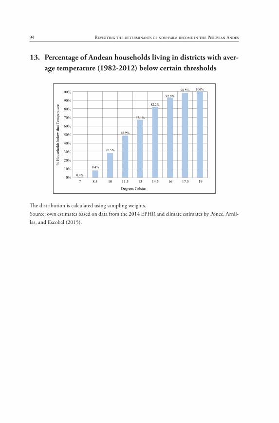
94 Revisiting the determinants of non-farm income in the Peruvian Andes
13. Percentage of Andean households living in districts with aver-age temperature (1982-2012) below certain thresholds
The distribution is calculated using sampling weights.Source: own estimates based on data from the 2014 EPHR and climate estimates by Ponce, Arnil-las, and Escobal (2015).
100%
90%
80%
70%
60%
50%
40%
30%
20%
10%
0%7
0.4%
8.5 10
% H
ouse
hold
s bel
ow th
at T
empe
ratu
re
11.5 13
Degrees Celsius
14.5 16 17.5 19
8.4%
28.5%
48.9%
67.1%
82.2%
92.6%
98.5% 100%


Revisiting the determinants of non-farm incomein the Peruvian Andes in a context of intraseasonal climate
variability and spatially widespread family networks
Edits completed in July 2018.