Revised Educational Note: Guidance for Investment ... · [email protected] /...

Members should be familiar with educational notes. Educational notes describe but do not recommend practice in illustrative situations. They do not constitute standards of practice

and are, therefore, not binding. They are, however, intended to illustrate the application (but not necessarily the only application) of the Standards of Practice, so there should be no

conflict between them. They are intended to assist actuaries in applying standards of practice in respect of specific matters. Responsibility for the manner of application of

standards of practice in specific circumstances remains that of the members.

Revised Educational Note

Investment Assumptions Used in the Valuation of Life and Health Insurance Contract Liabilities

Committee on Life Insurance Financial Reporting

September 2015

Document 215072

Ce document est disponible en français © 2015 Canadian Institute of Actuaries

1740-360 Albert, Ottawa, ON K1R 7X7 613-236-8196 613-233-4552

[email protected] / [email protected] cia-ica.ca

MEMORANDUM To: Members in the life insurance practice area From: Pierre Dionne, Chair

Practice Council

Rebecca Rycroft, Chair Committee on Life Insurance Financial Reporting

Date: September 16, 2015

Subject: Revised Educational Note: Guidance for Investment Assumptions Used in the Valuation of Life and Health Insurance Contract Liabilities

The Committee on Life Insurance Financial Reporting (CLIFR) received feedback related to implementation of the new Standards of Practice (effective on October 15, 2014). To address this feedback, CLIFR undertook, in 2015, to review the guidance provided related to the construction of the equilibrium risk-free market curve. The results of the work led to updating the attached educational note, specifically section 4.1. In addition, section 2 was updated to include a definition of fixed income assets and to amend the definition of non-fixed income assets. Appendix A and Appendix B have also been updated to reflect the new guidance. No other changes to the educational note were made.

This educational note has been prepared by CLIFR in accordance with the Institute’s Policy on Due Process for the Approval of Guidance Material other than Standards of Practice, and received final approval for distribution from the Practice Council on September 3, 2015.

As outlined in subsection 1220 of the Standards of Practice, “The actuary should be familiar with relevant Educational Notes and other designated educational material”. That subsection explains further that a “practice that the Educational Notes describe for a situation is not necessarily the only accepted practice for that situation and is not necessarily accepted actuarial practice for a different situation”. As well, “Educational Notes are intended to illustrate the application (but not necessarily the only application) of the standards, so there should be no conflict between them”.

Questions or comments regarding this educational note may be directed to Rebecca Rycroft at [email protected].

PD, RR

mailto:[email protected]

Revised Educational Note September 2015

3

Table of Contents 1 Introduction ......................................................................................................................... 4 2 Definitions ........................................................................................................................... 4 3 General Considerations in Setting Investment Assumptions .............................................. 5

3.1 Application of Judgment ............................................................................................... 5

3.2 Absence of New Business .............................................................................................. 5

3.3 Investment Time Horizon .............................................................................................. 6

4 Fixed Income Assets ............................................................................................................ 6 4.1 Development of Interest Rate Scenarios ...................................................................... 6

4.2 Foreign Currencies ......................................................................................................... 7

4.3 Stochastic Scenarios ...................................................................................................... 8

4.4 Credit Spreads ............................................................................................................... 9

4.4.1 Projection of Best Estimate Credit Spreads 11 4.4.2 Historical Averages 11 4.4.3 Data Sources for Historical Averages 12 4.4.4 Sample Historical Averages Based on Public Sources 13 4.4.5 Margins and Allowance for Asset Depreciation 14 4.4.6 Examples of Credit Spread Application 14 4.4.7 Other Assets 17

5 Non-Fixed Income Assets Supporting Liability Cash Flows ............................................... 17 5.1 Market Shift Assumptions ........................................................................................... 17

5.2 Application of the NFI Limitation ................................................................................ 18

5.2.1 Scope of Application 18 5.2.2 Definition of Cash Outflow 18 5.2.3 Derivation of the Discount Rate 18 5.2.4 Calculating the NFI Limit 19 5.2.5 NFI Limit 23 5.2.6 Considerations of Multiple NFI Asset Classes 23

5.3 Application of the NFI Limit for Contracts with Investment Pass-Through Features . 23

5.3.1 Participating Insurance 24 5.3.2 Universal Life Insurance 24

Appendix A…………………………………………………………………………………………………………………………..25 Appendix B…………………………………………………………………………………………………………………………..26


4

1 Introduction The primary purpose of this document is to provide guidance and support to actuaries in the application of standards of practice related to investment assumptions for financial reporting of life and health insurance.

Subsection 2330 of the Standards of Practice describes the prescribed interest rate scenarios to be used in the Canadian asset liability method (CALM), whereas subsection 2320 of the Standards of Practice sets out expectations related to the use of stochastic scenarios, which apply to the selection of stochastic interest rate scenarios. Subsection 2330 of the Standards of Practice also includes material related to the determination of future credit spreads on fixed income assets.

Subsection 2340 of the Standards of Practice sets out limitations on the use of non-fixed income (NFI) assets in CALM as well as specifying market shift assumptions to be used for NFI investments.

As a result of changes made to these subsections of the Standards of Practice in 2014, primarily related to future credit spreads and limitations on the use of NFI, additional guidance is being provided in this educational note. This guidance is intended to supplement information provided in other educational notes related to the application of these standards of practice to scenario testing under CALM.

2 Definitions Asset type for fixed income instruments includes government bonds (e.g., federal bonds, provincial bonds, and municipal bonds), corporate bonds, private placements, and mortgages, and may be further split between coupon-paying bonds and zero-coupon bonds.

Asset depreciation refers to expected losses due to credit-related events, including default, impairment, or restructuring, and includes loss of interest, loss of principal, and the expense of managing the credit-related event.

Asset subgroup refers to a group of assets with comparable characteristics such as asset type, quality rating, and/or term.

Credit spread or deterministic credit spread for a fixed income asset is the yield to maturity on that asset minus the yield to maturity on a risk-free fixed income asset with the same cash flow characteristics.

Investment policy refers to the terms and provisions of a company’s formal statement of investment policies and practices which sets out objectives, guidance, and limitations applying to investment activities.

Investment strategy refers to the investment approach taken or expected to be taken by the company in the application of its investment policy.

Net credit spread equals the deterministic credit spread less the expected losses due to asset depreciation.


5

Net credit spread after margin equals the net credit spread after application of the margin on credit spread and the margin on asset depreciation.

Fixed income assets refer to assets whose cash flows are contractually defined as to amount and timing.

Non-fixed income assets refer to assets that are not fixed income assets such as equities, primarily common stocks or private equities, real estate, timber holdings, agriculture, and other assets such as equity futures, exchange-traded funds or unit trusts.

Term (or term structure) refers to the relationship between bond yields and the term-to-maturity of a fixed income instrument. The term structure of interest rates is also referred to as a yield curve or market curve. Term structure will vary between coupon-paying and zero-coupon bonds.

Ultimate risk-free reinvestment rate (URR) refers to a stable interest rate at a given term (or range of terms) which is assumed to apply to investment activity undertaken at a future point in time.

3 General Considerations in Setting Investment Assumptions 3.1 Application of Judgment

The application of an investment policy to projected cash flows relies on assumptions so the translation of an investment policy into a future investment strategy to be used in scenario testing involves considerable scope for actuarial judgment.

Consultation with the asset-liability management (ALM) or investment department may provide valuable guidance towards choosing an investment strategy for a given scenario, but is unlikely to provide all the information required to develop reasonable projections. Examples of situations where there may be scope for actuarial judgment would include (i) consideration as to how the investment policy would be applied at the segmented level versus the total company level, (ii) assumptions as to how the investment policy would be applied after a material market correction, and (iii) consideration as to how the investment policy would be applied in the absence of new business.

The actuary is reminded that subsection 1130 of the Standards of Practice provides commentary on the application of actuarial judgment, including observations as to the spirit and intent of the standards of practice.

3.2 Absence of New Business

Paragraph 2330.05 of the Standards of Practice states:

The insurer’s expected practice would be determined without taking into consideration any business that could be issued after the valuation date (new sales) even for a valuation done on a going concern basis as described in paragraph 2130.02.

In applying this standard of practice, the assumed investment strategy would be expected to be reasonable in the absence of any new business. If the projected asset composition or the


6

projected asset purchases and sales appear unreasonable when new business is excluded, the actuary would need to consider using an alternative approach in the CALM projection.

The exclusion of new business would not be viewed as providing an additional margin or as compensation for making optimistic assumptions elsewhere.

3.3 Investment Time Horizon

The use of assets with material credit spreads or of NFI assets may be justified on the basis that they are suitable for long-term investing. The company’s investment policy would generally provide guidance as to how the company expects to effectively manage the risks associated with these assets. In performing CALM, the actuary would be expected to consider how the investment strategy would change over time for these assets.

The resulting investment strategy would be expected to respond to the shorter investment horizon over the projection period. A company’s current investment policy might provide indications as to how this might be expected to change over time. For example segments with shorter duration liabilities would typically have lower allocations to NFI assets.

4 Fixed Income Assets 4.1 Development of Interest Rate Scenarios

Paragraph 2330.09.1 of the Standards of Practice states:

In the base scenario,

risk-free interest rates effective after the balance sheet date would be equal to the forward interest rates implied by the equilibrium risk-free market curve at that date, for the first 20 years after the balance sheet date,

at and after the 60th anniversary from the balance sheet date, risk-free interest rates would be equal to the ultimate risk-free reinvestment rate – median,

at the 40th anniversary from the balance sheet date, the risk-free interest rates would be equal to 30% of the rates at the 20th anniversary plus 70% of the rates at the 60th anniversary,

between the 20th and 40th and between the 40th and 60th anniversaries, the risk-free interest rates would be determined using a uniform transition, and

credit spreads at all durations, would be the best estimate described in paragraph 2340.10.1.

The derivation of the base scenario can be summarized as shown in the following table.


7

Anniversary from Balance Sheet Date (Y years)

Risk-Free Interest Rate

Y ≤ 20th Forward interest rates implied by the equilibrium risk-free market curve at the balance sheet date

20th < Y < 40th Uniform transition between risk-free rates at the 20th and 40th anniversaries

Y= 40th 30% of the rates at the 20th anniversary plus 70% of the rates at the 60th anniversary

40th < Y < 60th Uniform transition between risk-free rates at the 40th and 60th anniversaries

Y ≥ 60th The ultimate risk-free reinvestment rate (URR)-median

In developing deterministic scenarios, any negative or zero forward rates would be set to 1 basis point.

In order to determine the 20-year forward rates out to year 20, an “equilibrium risk-free market curve” extending for at least 40 years from the balance sheet date is required. Risk-free interest rates are generally not observable in the market for very long terms (i.e., beyond 30 years). Beyond the 20-year point on the Canadian yield curve, interest rates are highly influenced by supply and demand constraints and the yield curve may be inverted as a result, which may not reflect the fundamental long-term interest rate risk. It would therefore be acceptable for the actuary to use observed market data for the first 20 years when developing a Canadian yield curve, and to apply an extrapolation beyond that period taking into account the historically observed long-term yields.

Appendix A presents an approach to developing 20-year implied forward rates for 20 years, using an extended spot yield curve. Under this approach, the extended spot yield curve has been developed by extending the spot rates beyond year 20 using a uniform transition from the 20-year spot rate to the long-term ultimate risk-free reinvestment rate-median (longURRmedian) in year 80.

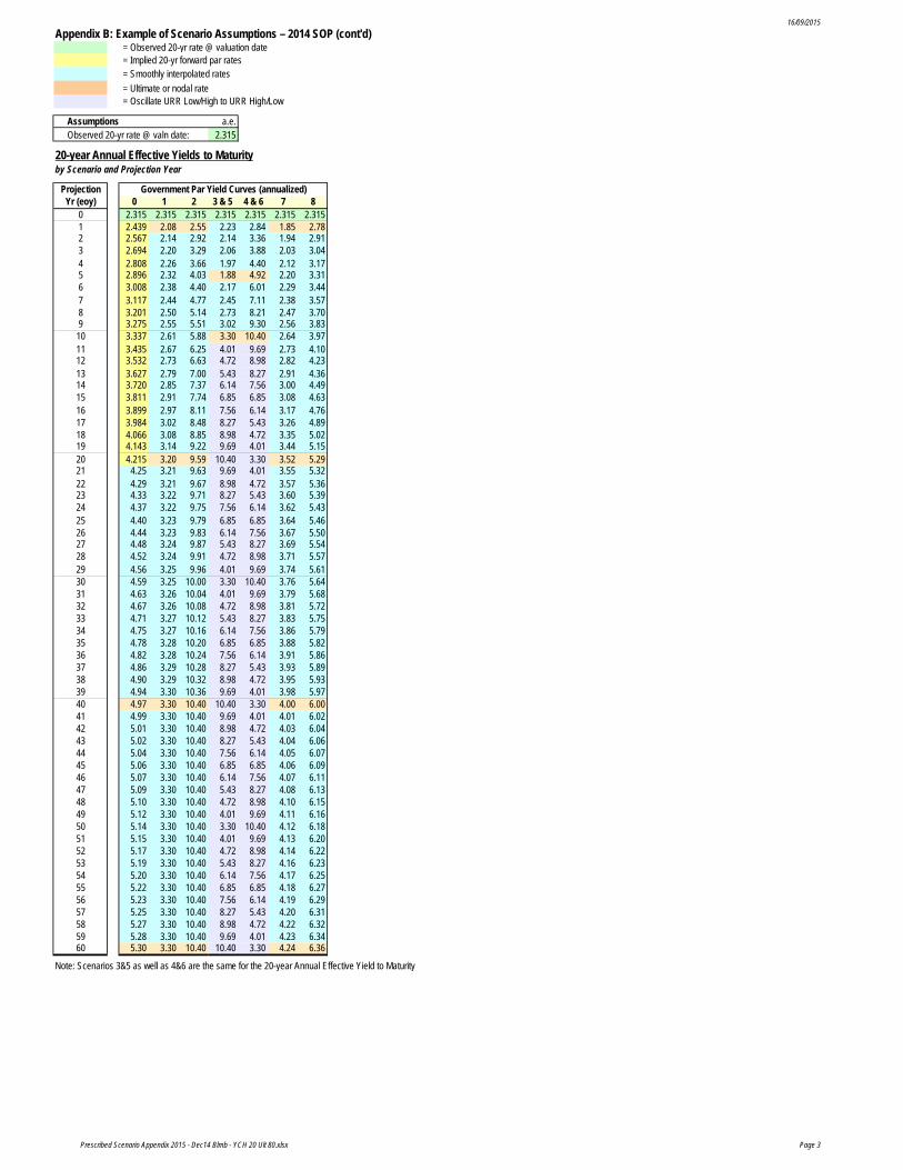
Appendix B illustrates the development of the 20-year annual effective par yields to maturity for a 60-year projection period, as derived for the base scenario and each of the prescribed scenarios, using the risk-free par yield curve in effect as at December 31, 2014.

4.2 Foreign Currencies



8

A scenario for a foreign country’s interest rates would be formulated independently of that for Canadian interest rates unless their positive historical correlation is expected to continue.

In addition, paragraph 2330.09.03 states:

The parameters in the base and prescribed scenarios, including maximum net credit spreads, apply to investments denominated in Canadian dollars. For the base and each prescribed scenario, the actuary would determine the corresponding parameters for investments denominated in a foreign currency from the historical relationship between investments denominated in that currency and investments denominated in the Canadian dollar if the expected continuance of that relationship so permits. Otherwise the actuary would devise independent scenarios for investments denominated in that currency.

The URRs promulgated by the Actuarial Standards Board would be appropriate for valuations using Canadian risk-free reinvestment assumptions. An actuary developing URRs for U.S. government bonds and many other developed countries would consider the Canadian URR as a starting point and make adjustments as appropriate. In making such adjustments, the actuary would consider rate history, market information, economic circumstances, and political conditions. For developing economies, the actuary would develop the URR after reviewing similar considerations, and may also consider different oscillation periods or other changes in the structure of the interest rate scenarios as appropriate.

4.3 Stochastic Scenarios


If the selection of scenarios is stochastic, then the actuary would adopt a scenario whose insurance contract liabilities are within the range defined by

the average of the insurance contract liabilities that are above the 60th percentile of the range of insurance contract liabilities for the selected scenarios, and

the corresponding average for the 80th percentile.

The actuary is reminded that the provision for adverse deviations (PfAD) for interest rate risk is defined as the difference between the resulting insurance contract liability and the insurance contract liability obtained under the base scenario (see paragraph 2330.09.2 of the Standards of Practice). Therefore the resulting insurance contract liability would be no less than that obtained under the base scenario, so as to avoid establishing a negative PfAD for interest rate risk.

Paragraph 2330.33 of the Standards of Practice states that

The actuary would adopt a scenario whose insurance contract liabilities are higher than the mid-point of the range described in paragraph 2320.51 whenever current long-term risk-free interest rates are near the limits or outside the range of long-term ultimate (risk-free) reinvestment rate-low to long-term ultimate (risk-free) reinvestment rate-high or whenever any of the considerations in paragraph 2330.31 exist.


9

The considerations stated in paragraph 2330.31 of the Standards of Practice are

the pattern of forecasted net cash flow in the base scenario is such that the classification of scenarios between favourable and unfavourable is unclear,

forecasted net cash flow is sensitive to the selection of interest rate scenarios,

the range of present values of forecasted net cash flow is wide, suggesting exposure to mismatch risk,

investment policy does not control mismatch risk,

asset-liability management is loose, or

flexibility to manage assets or liabilities is limited.

Where the conditions described in paragraph 2330.33 of the Standards of Practice exist, the actuary would hold insurance contract liabilities in the range of CTE(70) and CTE(80), subject to a minimum of the value obtained under the base scenario.

For example insurance contract liabilities for universal life (UL), which by their nature contain long-term liability cash flows sensitive to the interest rate scenarios, are normally exposed to mismatch risk, and as a result the actuary would set the insurance contract liabilities to be at least equal to CTE(70).

Another example would be a product where the projected liability cash flows oscillate between negative and positive under the base scenario. Such a pattern could make it unclear as to which scenarios would be favourable or unfavourable and such a product could be exposed to mismatch risk. In this case the actuary would set the insurance contract liabilities to be at least equal to CTE(70).

4.4 Credit Spreads


In all scenarios other than the base scenario, credit spreads include margins for adverse deviations as described in paragraph 2340.10.3. The actuary would also include an additional provision for adverse deviations by modifying the assumptions, if needed, on each fixed income asset purchased or sold on or after the 5th anniversary from the balance sheet date, such that

for assets purchased or sold on or after the 30th anniversary from the balance sheet date, the difference between the asset’s credit spread and its asset depreciation assumption is not larger than a maximum promulgated from time to time by the Actuarial Standards Board; and

for assets purchased or sold between the 5th and 30th anniversary from the balance sheet date, the difference between the asset’s credit spread and its asset depreciation assumption is not larger than using a uniform transition between the corresponding difference if purchased on the 5th anniversary from the balance sheet date and the promulgated maximum if purchased on the 30th anniversary from the balance sheet date.


10

Paragraphs 2340.10.1 to 2340.10.3 of the Standards of Practice state:

Fixed income assets: Credit Spreads

.10.1 The best estimate of credit spreads

would be the credit spreads available in the market at the balance sheet date,

at and after the 5th anniversary from the balance sheet date, would be based on long-term historical average credit spreads corresponding to assets by type, credit rating, and term, and

between the balance sheet date and the 5th anniversary, would be determined using a uniform transition.

.10.2 When choosing the best estimate of credit spreads based on long-term historical averages, the actuary would consider

using as long a period of history as practicable, and

adjusting the assumptions to reduce any inconsistencies that may arise from using different historical periods or sources of information for different asset types, credit ratings, or terms.

.10.3 The margin for adverse deviations in credit spreads would be

zero at the balance sheet date,

an addition or subtraction, as appropriate in aggregate, of 10% of the best estimate assumptions at and after the 5th anniversary from the balance sheet date, and

between the balance sheet date and the 5th anniversary, the margin for adverse deviations as percentage of the best estimate would be determined using a uniform transition.

The Standards of Practice provide for the use of deterministic credit spreads in all scenarios of risk-free interest rates, where the risk-free rates may be generated deterministically or stochastically.

To set the best estimate credit spread assumptions, the actuary would first define asset subgroups by considering factors such as asset type, credit rating, and term. For each asset within a particular asset subgroup, the best estimate credit spread for the first five years would be derived by using a uniform transition between the current credit spread at the balance sheet date and the historical average for that asset’s subgroup, over a five-year period.

A margin for adverse deviations grading from 0% to 10% over five years would be applied, as stipulated in paragraph 2340.10.3. As well, an assumption for expected asset depreciation and margin would be applied. The actuary would then determine whether the resulting net credit spread after margin for any fixed income asset exceeds the maximum defined in paragraph 2330.07.01. If the resulting net credit spread after margin exceeds the maximum for any assets within an asset subgroup, and if the excess causes a reduction in the insurance contract liabilities in aggregate, the actuary would include an additional provision for adverse deviations


11

by modifying the assumptions after the first five years so as to meet the conditions of paragraph 2330.07.01. Section 4.4.6 provides illustrations.

The following sections provide further guidance on credit spreads. Sections 4.4.1 to 4.4.4 provide guidance relating to setting best estimate credit spread assumptions, to which margins would then be applied.

4.4.1 Projection of Best Estimate Credit Spreads

For future asset purchases, the assumed credit spreads would start at asset subgroup values at the balance sheet date and then grade to historical averages over five years. Subsequent sales of any purchased assets would also use the assumed credit spreads.

For future sales of assets held at the balance sheet date, a number of approaches would be acceptable. The actuary would be consistent in the selection of a suitable approach for the circumstances and would avoid arbitrary shifts between approaches.

One approach (Approach I) would be to assume that credit spreads start at the actual asset-specific spreads at the balance sheet date and then grade to the best estimate credit spread assumptions derived from historical averages for each asset subgroup. This means that the difference between the calculated credit spread on an asset and the assumed credit spread for its particular asset subgroup would grade to zero over five years.

Another acceptable approach (Approach II) for future sales would be to assume that the best estimate credit spread for each asset held at the balance sheet date will remain a constant percentage of the best estimate assumption for the asset subgroup. The observed difference at the balance sheet date between the calculated credit spread on each asset and the credit spread for its particular asset subgroup would change over five years by the same percentage as the credit spread for the asset subgroup.

In any approach it would be expected that some assets would have credit spreads at the balance sheet date that are lower than the asset subgroup average, and other assets higher. The actuary would be cautious if individual assets were all consistently higher or lower than the asset subgroup average, and would consider whether the selection of asset subgroups and resulting approach is leading to a biased result.

4.4.2 Historical Averages

The historical averages for the credit spreads are to be used at and after the fifth anniversary from the balance sheet date and would be determined separately for each asset subgroup.

The best estimate historical average would be based on the longest available relevant period in order to capture a range of cycles in credit spreads. Generally at least 20 years of historical experience would be used. Although this is less historical information than was used for the development of risk-free rate scenarios, cycles in credit spreads can still be observed where credit spreads have widened out, and then returned to an average level relatively quickly. Given the relatively quick mean reversion and the use of a long historical period, it is recommended that outliers not be excluded from the data.


12

There may be instances where less than 20 years of experience is available. In this case, the limited number of years of historical information may still be sufficient if credit spreads have been stable during the period or have shown relatively short mean reversion periods after credit spreads have contracted or widened compared to historical averages. Under these circumstances, using the median, rather than the average, may also be considered.

When the asset subgroups are differentiated by term, public data sources often provide definitions of the terms “short”, “medium”, and “long”. For terms that fall between those provided in the public data, an estimation or interpolation approach may be necessary in order to obtain a full term structure.

4.4.3 Data Sources for Historical Averages

The actuary would refresh the historical averages for the asset subgroups as part of the regular assumption review. This section provides guidance on choosing the data sources for setting the historical averages.

Guidance developed in this section is for the Canadian context only. Information from the Bank of Canada is limited, but other data sources could also be used to determine assumptions for historical averages. For non-Canadian fixed income assets, the actuary would consider how to identify and apply relevant data sources appropriate for the circumstances.

For publicly traded fixed income assets, information from sources such as Bloomberg (from 1992) and PC Bond (from 1979) can be used to derive the historical averages. These sources generally provide more than 20 years of historical experience and provide information split by asset subgroups. Other sources may also be appropriate if they provide a sufficient amount of data and information split by asset subgroups. Some variation among sources is possible, particularly for corporate bonds. The actuary would consider the different sources available, assess the sources as to their suitability and ensure that the source used and its application are appropriate for the circumstances.

When the asset subgroups being used are broad-based and where credible public information is available, such as those illustrated in section 4.4.4, public information would be used. In other cases, the actuary would apply judgment in deciding how to combine their own company data with externally available information.

The actuary may consider refining the asset subgroups to a more granular level, such as differentiating by province within provincial bonds or using sector allocations within corporate bonds. In this case, the credit spreads may be determined by combining own company data and experience with externally available information. The actuary would ensure that the overall credit spreads remain consistent with externally available information for broad-based groups. The actuary would also consider whether the asset depreciation assumption for the broader asset subgroup is appropriate for the more granular subgroups.

For assets that aren’t publicly traded, such as private placements and mortgages, historical credit spread information is not readily available from public sources. For these assets, the asset subgroup would be split following a similar approach as used for the public bonds. The actuary would use their own company’s historical experience and relevant externally available information to determine an appropriate long-term historical credit spread assumption for each


13

asset subgroup. For example, external information could be used to assess the historical relationship between assets that are not publicly traded and those that are so as to ensure that the assumptions used for assets that are not publicly traded are consistent with assumptions used for publicly traded assets.

4.4.4 Sample Historical Averages Based on Public Sources

For illustrative and information purposes only, historical average credit spreads from PC Bond and Bloomberg are provided. The actuary is encouraged to reference the external sources directly for more complete information and to decide what is relevant for the circumstances. In addition, the actuary would consider the level of aggregation chosen as well as data availability and modelling capabilities.

Historical information available from PC Bond (from 1979) is based on series that are “short”, “medium”, and “long”. Additional series that show constant maturities may also be obtained and utilized for setting more granular valuation assumptions. Sample information from PC Bond as of September 2013 is shown below.

Short (1-5*)

Medium (5-10*)

Long (>10*)

Canada Provincial

(coupon) 0.32% 0.43% 0.61%

Corporate

AA 0.59% 0.73% 0.83% A 0.82% 1.00% 1.09% BBB 1.45% 1.55% 1.82%

Source: PC Bond

* As of September 2013, short, medium and long are approximately equivalent to terms of three years, seven years, and 22 years respectively.

The following illustrates the historical information available from Bloomberg (from 1992) as of December 2012:

2 year 5 year 7 year 10 year 20 year

Provincial 0.18% 0.35% 0.44% 0.56% 0.62%

Corp AA 0.42% 0.60% 0.65% 0.70% 0.81%

Corp A 0.66% 0.80% 0.85% 0.96% 1.17%

Corp BBB 1.05% 1.29% 1.39% 1.54% 1.77%

Source: Bloomberg


14

4.4.5 Margins and Allowance for Asset Depreciation

A margin for adverse deviations for credit spread grading from 0% at the balance sheet date to 10% over five years would be applied, as stipulated in paragraph 2340.10.3. As well, an assumption for expected asset depreciation and margin would be applied.

The difference between the credit spread and asset depreciation assumptions after margin (i.e., net credit spread after margin) between the fifth and 30th anniversary is subject to the maximum defined in paragraph 2330.07.01. Subsection 2340 of the Standards of Practice describes the asset depreciation assumption for fixed income assets. Although it may be conservative for a reinvestment assumption, the maximum defined in paragraph 2330.07.01 may not be conservative in a disinvestment situation. In this case, the actuary would test whether applying the maximum defined in paragraph 2330.07.01 increases or decreases insurance contract liabilities. The maximum would only be applied in the situation where insurance contract liabilities increase.

4.4.6 Examples of Credit Spread Application

Examples applicable to two assets in two different asset subgroups held at the balance sheet date are provided below. The examples illustrate the derivation of credit spreads in the fair value calculation for any future sale of the assets.

In both examples, the maximum defined in paragraph 2330.07.01 is assumed to be 80 bps, which is consistent with the Standards of Practice published in 2014.

Assets at the Balance Sheet Date - Asset Subgroup 1

The two assets have best estimate credit spreads of 40 basis points (bps) and 60 bps respectively at the balance sheet date. The best estimate credit spread assumption for this asset subgroup is 55 bps at the balance sheet date with a long-term historical average of 50 bps. The margin for credit spreads is a subtraction of 10% (assuming that applying a negative margin increases the insurance contract liabilities in aggregate). This example assumes also that the best estimate asset depreciation assumption is 4 bps and the margin for asset depreciation is 50%.

As a result, using Approach I as defined in section 4.4.1, over the initial five-year period:

• The best estimate credit spread assumption for:

o Asset A would grade from 40 bps to 50 bps over a five-year period, and

o Asset B would grade from 60 bps to 50 bps over a five-year period.

• The credit spread assumption after credit spread margin for:



• The assumption for net credit spread after margin for:


15



After the initial five-year period, the best estimate credit spread assumption for Asset A and Asset B would remain level at 50 bps. Similarly, the net credit spread after margin for Asset A and Asset B would remain level at 39 bps because it is not impacted by the maximum defined in paragraph 2330.07.01.

The following table illustrates the net credit spread after margin for these two assets, assuming a linear uniform transition:

End of Year

Asset 0 1 2 3 4 5 6 … 20 … 30

Asset A 34.0 35.2 36.2 37.2 38.2 39.0 39.0 … 39.0 … 39.0

Asset B 54.0 50.8 47.8 44.8 41.8 39.0 39.0 … 39.0 … 39.0

If Approach II as defined in Section 4.4.1 is used, from the 5th anniversary and onwards,

• the best estimate credit spread assumption would be 36.43 bps for Asset A and 54.54 bps for Asset B; and

• the net credit spread after margin would be 26.7 bps for Asset A and 43.1 bps for Asset B.

Assets at the Balance Sheet Date - Asset Subgroup 2

In the second example, the two assets have best estimate credit spreads of 150 basis points (bps) and 110 bps respectively at the balance sheet date. The best estimate credit spread assumption for this asset subgroup is 135 bps at the balance sheet with a long-term historical average of 130 bps. The margin for credit spreads is a subtraction of 10% (assuming that applying a negative margin increases the insurance contract liabilities in aggregate). This example assumes also that the best estimate asset depreciation assumption is 20 bps and the margin for asset depreciation is 50%.

As a result, using Approach I as defined in section 4.4.1, over the initial five-year period: • The best estimate credit spread assumption for:

o Asset A would grade from 150 bps to 130 bps over a five year period, and o Asset B would grade from 110 bps to 130 bps over a five year period.

1 40 bps x (1 – 0%) – 4 bps x (1+50%) 2 50 bps x (1 – 10%) – 4 bps x (1+50%) 3 40 bps x 50 bps/55 bps 4 60 bps x 50 bps/55 bps


16

• The credit spread assumption after credit spread margin for: o Asset A would grade from 150 bps to 117 bps over a five year period, and o Asset B would grade from 110 bps to 117 bps over a five year period.

• The assumption for net credit spread after margin for: o Asset A would grade from 120 bps to 87 bps over a five year period, and o Asset B would grade from 80 bps to 87 bps over a five year period.

After the initial five year period, the best estimate credit spread assumption for Asset A and Asset B would remain at 130 bps. Since it is impacted by the maximum defined in paragraph 2330.07.01, the net credit spread after margin for Asset A and Asset B would grade from 87 bps after year 5 to 80 bps at the end of year 30.

The following table illustrates the net credit spread after margin for these two assets, assuming a linear uniform transition to the maximum defined in paragraph 2330.07.01:

End of Year

Asset 0 1 2 3 4 5 6 … 20 … 30

Asset A 120.0 113.1 106.3 99.7 93.3 87.0 86.7 … 82.8 … 80.0

Asset B 80.0 81.7 83.3 84.7 85.9 87.0 86.7 … 82.8 … 80.0

If Approach II as defined in section 4.4.1 is used, at the fifth anniversary,

• the best estimate credit spread assumption would be 144.4 bps for Asset A and 105.9 bps for Asset B; and

• the net credit spread after margin would be 100.0 bps for Asset A and 65.3 bps for Asset B.

Since Asset A is impacted by the maximum defined in paragraph 2330.07.01, the net credit spread after margin for Asset A would grade from 100 bps after year 5 to 80 bps at the end of year 30. The net credit spread for Asset B remains level at 65.3 bps after the initial five-year period.

Reinvestments

For any new purchases, the credit spread assumption for the asset subgroup as a whole would apply.

For Asset Subgroup 1 and Asset Subgroup 2 described above, the following assumptions for net credit spread after margin would apply:


17

End of Year

Category 0 1 2 3 4 5 6 … 20 … 30

Subgroup 1 49.0 46.9 44.9 42.9 40.9 39.0 39.0 … 39.0 … 39.0

Subgroup 2 105.0 101.3 97.7 94.1 90.5 87.0 86.7 … 82.8 … 80.0

For practical reasons, other approaches that include simplifications and/or approximations may also be used, particularly if the results of the valuation are not materially impacted.

4.4.7 Other Assets

For assets with unique characteristics (i.e., that are different from the assets belonging to the established asset subgroups), the actuary could develop asset subgroups that would be unique to these assets. The actuary would then still determine the current credit spread at the balance sheet date, and a best estimate credit spread from historical averages for that unique asset subgroup. Public information may be more limited under these circumstances, with greater reliance being placed on own company data, so the actuary would face considerations similar to those for private placements and mortgages, as discussed in section 4.4.3.

5 Non-Fixed Income Assets Supporting Liability Cash Flows 5.1 Market Shift Assumptions


Where the best estimate for a class of non-fixed income assets is based on reliable historical data, the margin for adverse deviations in the assumption of non fixed-income capital gains would be 20% of the best estimate plus an assumption that those assets change in value at the time when the change is most adverse. That time would be determined by testing, but usually would be the time when their book value is largest. The assumed change as a percentage of market value

of a diversified portfolio of North American common shares would be 30%, and

of any other portfolio would be in the range of 20% to 50% depending on the volatility relative to a diversified portfolio of North American common shares.

For any portfolio other than North American common shares, the lower end of the range would apply when the volatility for the reference benchmark is relatively low. For example, for broad-based real estate portfolios, the annualized volatility would be expected to be significantly lower than that for equity funds; therefore a market shift percentage at the lower end of the range may be appropriate.

The high end of the range for market shift assumptions would apply to highly volatile NFI assets. Generally, the MfADs for scenario-tested assumptions, such as the market shift assumption, would be selected to approximate a CTE(60) to CTE(80) insurance contract liability.


18

5.2 Application of the NFI Limitation


If non-fixed income assets are used to support liability cash flows that are not substantially linked to returns on non-fixed income assets, the actuary would include an additional provision for adverse deviations by modifying the assumed investment strategy in the scenario adopted prior to considering this provision for adverse deviations, if needed, so that the amount of non-fixed income assets supporting such liability cash flows at the balance sheet date and at each duration in the projection does not exceed the amount required to support 20% of cash outflows for the first 20 years and 75% thereafter, where cash outflows are the greater of the annual liability cash flows and zero in each forecast period. This modification of the assumed investment strategy would be applied at each duration independently.

5.2.1 Scope of Application

The limitation on the use of NFI assets would be applied to the adopted scenario after CALM scenario testing is completed. The actuary would not be expected to apply the NFI limitation to all CALM scenarios.

For contracts without substantial investment pass-through features, the limit on the use of NFI assets applies to the entire contract. For contracts with substantial investment pass-through features, the limit only applies to the portion of the liability cash flows that are not substantially linked to returns on NFI assets. Additional information on bifurcating contracts with investment pass-through features into components where the NFI limitation applies and where it does not is provided in section 5.3 below.

5.2.2 Definition of Cash Outflow

The annual liability cash outflow is equal to the total cash outflows, which include benefits and expenses less premiums. When the sum of benefits and expenses is greater than premiums, the net balance is positive. When the sum is less than premiums, the net balance is negative. The cash outflow, referred to in paragraph 2340.14.1, will equal the annual liability cash flow when the balance is positive and will equal zero when the balance is negative.

5.2.3 Derivation of the Discount Rate

The discount rate described in this section is used in calculating the maximum NFI at a given projection period as illustrated in section 5.2.4. In deriving the discount rate, the actuary would use the spot rate implied by the net NFI asset returns. The net NFI asset returns are calculated for each projection period based on the best estimate NFI growth and income assumptions, net of the investment expenses and MfADs. When calculating the maximum NFI for a given projection period, the actuary would apply the market correction MfAD at the most adverse time.

The market correction MfAD used in the maximum NFI calculation is independent of the market correction MfAD used in the CALM scenario testing. In principle, the timing of the correction would be determined independently for every projection period’s maximum NFI calculation. Therefore the timing of the CALM-related market correction MfAD is not relevant for the


19

purpose of calculating the maximum NFI. Note that even though the timing of the market correction MfAD may vary between CALM scenario testing and the maximum NFI calculation, the magnitude of the MfAD will not vary.

For discount rate it, depicted in figures 2A, 2B, and 2C, the actuary would account for the market correction MfAD when deriving the discount rate. For discount rate rt, depicted in figure 2D, the market correction MfAD would not be included as it is already explicitly accounted for in the notation.

5.2.4 Calculating the NFI Limit

As stated in paragraph 2340.14.1, the maximum amount of NFI assets is calculated by discounting “20% of cash outflows for the first 20 years and 75% thereafter, where cash outflows are the greater of the annual liability cash flows and zero in each forecast period.”

This is illustrated in figure 1.

Figure 1: 20-20-75 Constraint

The 20-20-75 limit is calculated at each projection period independently. In figure 2A, the NFI holdings at time 0 are limited to the present value of cash outflows supported by NFI at time 0 (MaxNFI0). In figure 2B, NFI holdings at time 1 are limited to the present value of cash outflows supported by NFI at time 1 (MaxNFI1). In figure 2C, NFI holdings at time 30 are limited to the present value of cash outflows supported by NFI at time 30 (MaxNFI30).


20

Figure 2A: Maximum NFI at Time 0

Figure 2B: Maximum NFI at Time 1


21

Figure 2C: Maximum NFI at Time 30

Repeating this process for all forecast periods in a projection creates a durational vector of constraints. These constraints limit the amount of NFI assets used in the insurance contract liability calculation.

In practice, the market correction would usually occur at the time when the NFI book value is its largest. In the determination of the maximum NFI holdings at an arbitrary time s (MaxNFIs), the NFI book value is at its largest at time s. Therefore, if the former condition holds, the market correction used in calculating MaxNFIs would occur at time s. The notation can then be simplified as depicted below in figure 2D.

Figure 2D: Maximum NFI with Assumed Market Correction MfAD Timing

If we assume that the investment strategy is to invest in NFI assets at the 20-20-75 limit for all projection periods in the adopted scenario, and apply a market correction MfAD of 30% in the


22

first year of the projection, we can illustrate the NFI assets as a percentage of total assets in figure 3. Note that the NFI proportion converges to 20/(1-MfAD)%.

There is the potential for an increase in NFI assets caused by the disinvestment of fixed income assets and reinvestment of NFI assets immediately following the market correction. This example is meant to illustrate the interaction between the 20-20-75 limit and the market correction MfAD within the adopted scenario. It would not be interpreted as recommending an investment strategy assumption.

Figure 3: NFI Assets as a Percentage of Total Assets


23

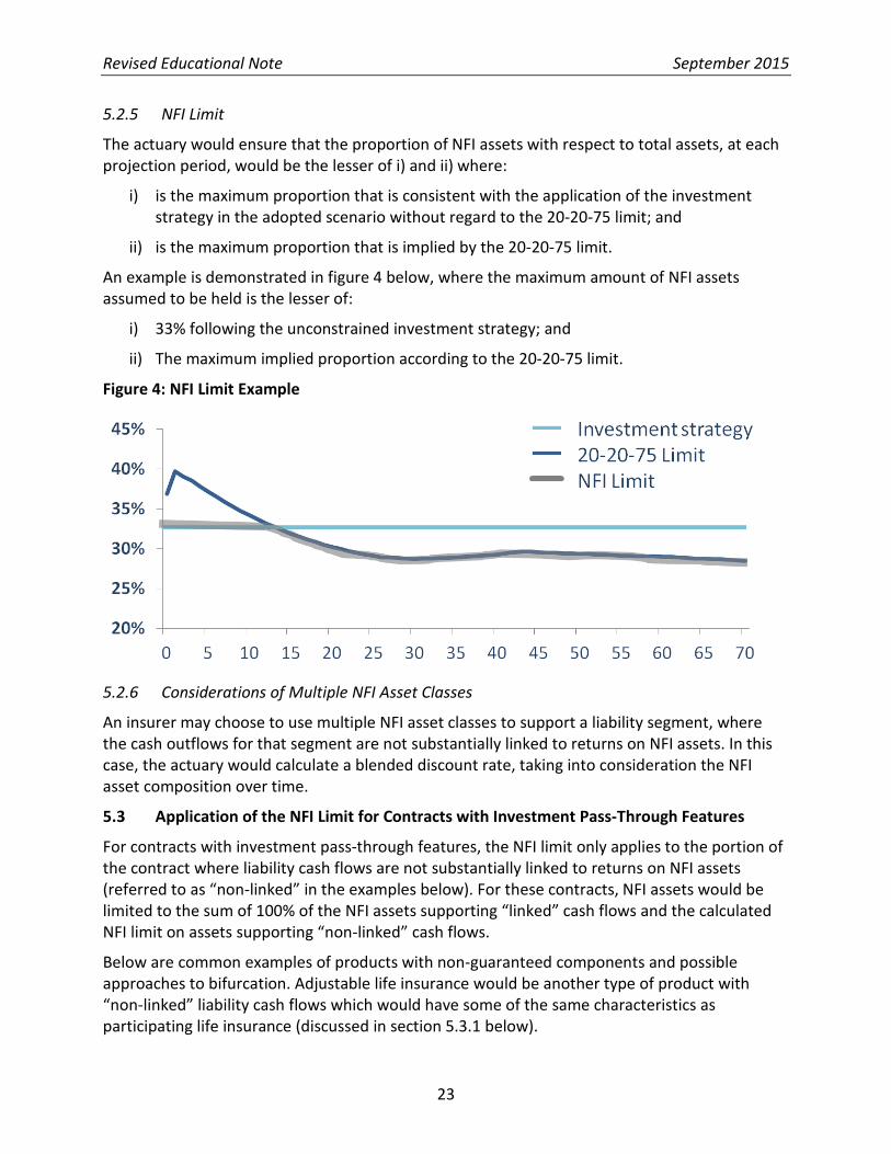
5.2.5 NFI Limit

The actuary would ensure that the proportion of NFI assets with respect to total assets, at each projection period, would be the lesser of i) and ii) where:

i) is the maximum proportion that is consistent with the application of the investment strategy in the adopted scenario without regard to the 20-20-75 limit; and

ii) is the maximum proportion that is implied by the 20-20-75 limit.

An example is demonstrated in figure 4 below, where the maximum amount of NFI assets assumed to be held is the lesser of:

i) 33% following the unconstrained investment strategy; and

ii) The maximum implied proportion according to the 20-20-75 limit.

Figure 4: NFI Limit Example

5.2.6 Considerations of Multiple NFI Asset Classes

An insurer may choose to use multiple NFI asset classes to support a liability segment, where the cash outflows for that segment are not substantially linked to returns on NFI assets. In this case, the actuary would calculate a blended discount rate, taking into consideration the NFI asset composition over time.

5.3 Application of the NFI Limit for Contracts with Investment Pass-Through Features

For contracts with investment pass-through features, the NFI limit only applies to the portion of the contract where liability cash flows are not substantially linked to returns on NFI assets (referred to as “non-linked” in the examples below). For these contracts, NFI assets would be limited to the sum of 100% of the NFI assets supporting “linked” cash flows and the calculated NFI limit on assets supporting “non-linked” cash flows.

Below are common examples of products with non-guaranteed components and possible approaches to bifurcation. Adjustable life insurance would be another type of product with “non-linked” liability cash flows which would have some of the same characteristics as participating life insurance (discussed in section 5.3.1 below).


24

5.3.1 Participating Insurance

Participating insurance contracts can include both linked and non-linked liability cash flows. For example, the death benefit cash flows associated with the basic sum insured and past dividends paid out as vested paid-up insurance would be considered non-linked. The liability cash flows associated with future dividends, to the extent that the company can adjust the dividend based on NFI experience, would be considered linked. This determination would be irrespective of the form in which dividends are paid. Policyholder reasonable expectations and delays/smoothing in the process of updating dividend scales might prevent the full transfer of NFI experience.

In calculating the maximum amount of NFI assets at a given projection period, the actuary would take into account all guaranteed liability cash flows projected since the valuation date including those associated with assumed dividends. For example, within a projection, if a dividend is paid out in the form of vested paid-up insurance, the non-linked liability cash flows would include these amounts. In principle, a projection of future non-linked liability cash flows would be recalculated at each projection period, reflecting the accumulated paid-up insurance assumed in the projection since the valuation date.

5.3.2 Universal Life Insurance

UL insurance contracts include an investment component where policyholder funds may be placed in one or more NFI-linked investment options. To the extent that this occurs, all NFI pass-through inherent in the liability cash flows would be considered linked. All other liability cash flows would be considered non-linked and thus subject to the NFI limit. In certain cases, the classification of liability cash flows may not be straightforward. A common example is when the UL death benefit is level. Under a level death benefit option, the net amount at risk (NAAR) is the difference between a constant total death benefit and the policyholder funds. Thus, the death benefit cash flows may include both linked and non-linked components. The actuary would use judgment to develop an estimate of the non-linked liability cash flows for these policies. One approach would be to project the NAAR based on the valuation assumptions for the interest credited on policyholder funds, and to consider the resulting cash flows as guaranteed.

Another consideration related to UL contracts are the margins earned on investment funds. Margins are the excess of income earned on assets supporting investment funds over the interest credited to policyholder funds, net of commissions and other expenses. The classification of the margins cash flows would depend on the nature of the investment funds. The margin cash flows associated with investment funds that are based on NFI-linked investment options would be considered linked. The margin cash flows associated with investment funds that are based on a fixed return would be considered non-linked and thus subject to the NFI limit.

16/09/2015

Prescribed Scenario Appendix 2015 - Dec14 Blmb - YCH 20 Ult 80.xlsx Page 1

Appendix A: Derivation of Forward Par Curve - 2014 SOP, revised Ed Note 2015

Par Yields, Spot Rates, Forward Spots, and Forward Par Yields Illustration: 1- and 20-yr Terms all rates annualized

Define a spot rate zn as the yield on a zero-coupon bond maturing in n periods. Observed Rates by Term Implied Forwards by YearGiven an observed par yield curve pn, the spot curve zn is derived recursively: December 31st, 2014 (Bloomberg) Spots Par Yields

Term Par an-1 Spots Adj Spot 1-yr 20-yr 1-yr 20-yrFormula 1: 1 20

0 0.989% 2.419% 2 0.989% 2.315%1 0.989% 0.000 0.989% 0.989% 1.037% 2.541% 1.037% 2.439%2 1.013% 0.990 1.013% 1.013% 1.189% 2.666% 1.189% 2.567%3 1.071% 1.970 1.072% 1.072% 1.508% 2.789% 1.508% 2.694%

Define a forward spot F(n,m) as the zn on a zero purchased m periods from now. 4 1.178% 2.939 1.180% 1.180% 2.004% 2.899% 2.004% 2.808%Given a spot curve zn, the implied Forward spots F(n,m) are derived via the relation: 5 1.338% 3.893 1.345% 1.345% 1.757% 2.990% 1.757% 2.896%

6 1.405% 4.828 1.413% 1.413% 1.899% 3.098% 1.899% 3.008%Formula 2: 7 1.472% 5.748 1.482% 1.482% 2.389% 3.204% 2.389% 3.117%

8 1.579% 6.650 1.595% 1.595% 2.628% 3.290% 2.628% 3.201%9 1.687% 7.531 1.710% 1.710% 2.873% 3.369% 2.873% 3.275%10 1.794% 8.389 1.825% 1.825% 2.436% 3.440% 2.436% 3.337%

The corresponding forward par yields FP(n,m) are then derived via the formula 11 1.846% 9.224 1.881% 1.881% 2.557% 3.538% 2.557% 3.435%12 1.898% 10.038 1.937% 1.937% 2.680% 3.635% 2.680% 3.532%

Formula 3: 13 1.950% 10.833 1.994% 1.994% 2.806% 3.731% 2.806% 3.627%14 2.002% 11.606 2.052% 2.052% 2.935% 3.825% 2.935% 3.720%15 2.055% 12.359 2.110% 2.110% 3.068% 3.918% 3.068% 3.811%16 2.107% 13.090 2.170% 2.170% 3.205% 4.008% 3.205% 3.899%

A sample process is outlined below; sample 1- and 20-year rates are illustrated at right. 17 2.159% 13.799 2.230% 2.230% 3.346% 4.097% 3.346% 3.984%18 2.211% 14.487 2.292% 2.292% 3.491% 4.183% 3.491% 4.066%19 2.263% 15.152 2.355% 2.355% 3.642% 4.267% 3.642% 4.143%20 2.315% 15.794 2.419% 2.419% 3.432% 4.349% 3.432% 4.215%21 2.318% 16.414 2.418% 2.467% 1 3.529% 4.445% 3 3.529% 4.309%

Construction of Implied Forward Par Yield Curves - Steps 22 2.321% 17.020 2.418% 2.515% 3.625% 4.542% 3.625% 4.403%23 2.325% 17.611 2.418% 2.563% 3.722% 4.639% 3.722% 4.497%

Step 1: Obtain current par yield curve from an appropriate source (e.g., Bloomberg). 24 2.328% 18.188 2.419% 2.611% 3.818% 4.736% 3.818% 4.591%25 2.331% 18.752 2.420% 2.659% 3.915% 4.832% 3.915% 4.685%

Step 2: Interpolate the par yield curve where yields are not directly available. 26 2.334% 19.302 2.421% 2.707% 4.011% 4.929% 4.011% 4.779%27 2.337% 19.839 2.422% 2.755% 4.108% 5.026% 4.108% 4.873%

Step 3: Derive the equivalent spot rate curve using Formula 1. 28 2.341% 20.363 2.424% 2.803% 4.205% 5.123% 4.205% 4.967%29 2.344% 20.874 2.426% 2.851% 4.301% 5.220% 4.301% 5.061%

Step 4: Beyond year 20, calculate an adjusted spot rate by using a uniform 30 2.347% 21.373 2.428% 2.899% 4.398% 5.317% 4.398% 5.155%transition from the spot rate in year 20 to the median long-term ultimate risk-free 31 2.347% 21.860 2.425% 2.947% 4.495% 5.414% 4.495% 5.249%reinvestment rate-median (longURRmedian) in year 80. 32 2.347% 22.336 2.423% 2.995% 4.592% 5.511% 4.592% 5.343%

33 2.347% 22.801 2.420% 3.043% 4.688% 5.608% 4.688% 5.437%Step 5: Derive the implied forward spots using Formula 2. 34 2.347% 23.255 2.418% 3.091% 4.785% 5.705% 4.785% 5.531%

35 2.347% 23.699 2.416% 3.139% 4.882% 5.802% 4.882% 5.626%Step 6: Determine the equivalent implied forward par yields using Formula 3. 36 2.347% 24.132 2.414% 3.187% 4.979% 5.899% 4.979% 5.720%

37 2.347% 24.556 2.412% 3.235% 5.076% 5.996% 5.076% 5.814%38 2.347% 24.970 2.411% 3.283% 5.173% 6.093% 5.173% 5.909%39 2.347% 25.374 2.409% 3.331% 5.269% 6.190% 5.269% 6.003%

Notes 40 2.347% 25.770 2.408% 3.379% 5.366% 6.287% 5.366% 6.097%Spots 41 2.347% 26.156 2.406% 3.427% 5.463% 6.384% 5.463% 6.192%

1. Spot rate begins to grade to Median URR = 5.30% 42 2.347% 26.533 2.405% 3.475% 5.560% 6.482% 5.560% 6.286%2. For each term, the time-0 forward spot equals the observed spot for that term. 43 2.347% 26.902 2.403% 3.523% 5.657% 6.579% 5.657% 6.381%3. For each term, only the first 20 forwards are used in the Base Scenario. 44 2.347% 27.262 2.402% 3.571% 5.754% 6.676% 5.754% 6.475%

45 2.347% 27.614 2.401% 3.619%46 2.347% 27.958 2.400% 3.667%47 2.347% 28.293 2.398% 3.715%

11

11

−

+

+=

++

n

mm

nmnm

zzmnF

)()(),(

111

1

1

1

1

−

+−

+=

∑−

=

−

n

n

k

kkn

nn

zp

pz))((

)(

∑=

−

−

+

+−= n

k

k

n

mkF

mnFmnFP

11

11

)),((

)),((),(

16/09/2015


Appendix B: Example of Scenario Assumptions – 2014 SOP

Interest Rate Scenarios

Scenario Description

0 0<Y<1 1 2-19 20 21-39 40 41-59 60

0 Uniform Transition

30%*20 yr +70%*60 yr

Uniform Transition

Median URR (4%/5.3%)

1 B/S Uniform Transition 90% * B/S Uniform

Transition10%* B/S + 90%*40 yr

Uniform Transition


Transition10%* B/S + 90%*40 yr

Uniform Transition

3

4

5

6


Transition

80%(30%* B/S + 70%* Median

URR)

Uniform Transition

80%(10%* B/S + 90%* Median

URR)

Uniform Transition

80%*Median URR


Transition

120%(30%* B/S + 70%* Median

URR)

Uniform Transition

120%(10%* B/S + 90%* Median

URR)

Uniform Transition

120%*Median URR

B/S = rates at Balance Sheet date (i.e., projection year 0)

Projection Year

Base Interest Rate Scenario (forward rates for first 20 years based on the current yield curve; Nodal point at Year 40; Prescribed Median by Year 60)Move to 90% of Current by Year 1; Nodal point at Year 20; Prescribed Minimums by Year 40Move to 110% of Current by Year 1; Nodal point at Year 20; Prescribed Maximums by Year 40

Yield Curve Movements In Full Cycles (Down/Up/Down/Up/Down/Up)

Yield Curve Movements In Full Cycles (Up/Down/Up/Down/Up/Down)

Implied Forwards for first 20 years

Low URR (1.4%/3.3%)

High URR (10%/10.4%)

Oscillate between URR Low and URR High every 10 years (full cycle of 20 years), S/T rate is 60% of L/T rate

Oscillate between URR High and URR Low every 10 years (full cycle of 20 years), S/T rate is 60% of L/T rate

Same as 3 except S/T rate moves in 20% annual steps from 40% to 120% of L/T rate

Inversions and Yield Curve Movements In Full Cycles (Down/Up/Down/Up/Down/Up)Move to 80% of Current by Year 1; Nodal points at Years 20 and 40; 80% of Prescribed Median by Year 60Move to 120% of Current by Year 1; Nodal points at Years 20 and 40; 120% of Prescribed Median by Year 60

Inversions and Yield Curve Movements In Full Cycles (Up/Down/Up/Down/Up/Down)

Same as 5 except S/T rate moves in 20% annual steps from 120% to 40% of L/T rate

16/09/2015


Appendix B: Example of Scenario Assumptions – 2014 SOP (cont'd) = Observed 20-yr rate @ valuation date = Implied 20-yr forward par rates = Smoothly interpolated rates = Ultimate or nodal rate = Oscillate URR Low/High to URR High/Low

Assumptions a.e.Observed 20-yr rate @ valn date: 2.315

20-year Annual Effective Yields to Maturityby Scenario and Projection Year

Projection Government Par Yield Curves (annualized)Yr (eoy) 0 1 2 3 & 5 4 & 6 7 8

0 2.315 2.315 2.315 2.315 2.315 2.315 2.3151 2.439 2.08 2.55 2.23 2.84 1.85 2.782 2.567 2.14 2.92 2.14 3.36 1.94 2.913 2.694 2.20 3.29 2.06 3.88 2.03 3.044 2.808 2.26 3.66 1.97 4.40 2.12 3.175 2.896 2.32 4.03 1.88 4.92 2.20 3.316 3.008 2.38 4.40 2.17 6.01 2.29 3.447 3.117 2.44 4.77 2.45 7.11 2.38 3.578 3.201 2.50 5.14 2.73 8.21 2.47 3.709 3.275 2.55 5.51 3.02 9.30 2.56 3.83

10 3.337 2.61 5.88 3.30 10.40 2.64 3.9711 3.435 2.67 6.25 4.01 9.69 2.73 4.1012 3.532 2.73 6.63 4.72 8.98 2.82 4.2313 3.627 2.79 7.00 5.43 8.27 2.91 4.3614 3.720 2.85 7.37 6.14 7.56 3.00 4.4915 3.811 2.91 7.74 6.85 6.85 3.08 4.6316 3.899 2.97 8.11 7.56 6.14 3.17 4.7617 3.984 3.02 8.48 8.27 5.43 3.26 4.8918 4.066 3.08 8.85 8.98 4.72 3.35 5.0219 4.143 3.14 9.22 9.69 4.01 3.44 5.1520 4.215 3.20 9.59 10.40 3.30 3.52 5.2921 4.25 3.21 9.63 9.69 4.01 3.55 5.3222 4.29 3.21 9.67 8.98 4.72 3.57 5.3623 4.33 3.22 9.71 8.27 5.43 3.60 5.3924 4.37 3.22 9.75 7.56 6.14 3.62 5.4325 4.40 3.23 9.79 6.85 6.85 3.64 5.4626 4.44 3.23 9.83 6.14 7.56 3.67 5.5027 4.48 3.24 9.87 5.43 8.27 3.69 5.5428 4.52 3.24 9.91 4.72 8.98 3.71 5.5729 4.56 3.25 9.96 4.01 9.69 3.74 5.6130 4.59 3.25 10.00 3.30 10.40 3.76 5.6431 4.63 3.26 10.04 4.01 9.69 3.79 5.6832 4.67 3.26 10.08 4.72 8.98 3.81 5.7233 4.71 3.27 10.12 5.43 8.27 3.83 5.7534 4.75 3.27 10.16 6.14 7.56 3.86 5.7935 4.78 3.28 10.20 6.85 6.85 3.88 5.8236 4.82 3.28 10.24 7.56 6.14 3.91 5.8637 4.86 3.29 10.28 8.27 5.43 3.93 5.8938 4.90 3.29 10.32 8.98 4.72 3.95 5.9339 4.94 3.30 10.36 9.69 4.01 3.98 5.9740 4.97 3.30 10.40 10.40 3.30 4.00 6.0041 4.99 3.30 10.40 9.69 4.01 4.01 6.0242 5.01 3.30 10.40 8.98 4.72 4.03 6.0443 5.02 3.30 10.40 8.27 5.43 4.04 6.0644 5.04 3.30 10.40 7.56 6.14 4.05 6.0745 5.06 3.30 10.40 6.85 6.85 4.06 6.0946 5.07 3.30 10.40 6.14 7.56 4.07 6.1147 5.09 3.30 10.40 5.43 8.27 4.08 6.1348 5.10 3.30 10.40 4.72 8.98 4.10 6.1549 5.12 3.30 10.40 4.01 9.69 4.11 6.1650 5.14 3.30 10.40 3.30 10.40 4.12 6.1851 5.15 3.30 10.40 4.01 9.69 4.13 6.2052 5.17 3.30 10.40 4.72 8.98 4.14 6.2253 5.19 3.30 10.40 5.43 8.27 4.16 6.2354 5.20 3.30 10.40 6.14 7.56 4.17 6.2555 5.22 3.30 10.40 6.85 6.85 4.18 6.2756 5.23 3.30 10.40 7.56 6.14 4.19 6.2957 5.25 3.30 10.40 8.27 5.43 4.20 6.3158 5.27 3.30 10.40 8.98 4.72 4.22 6.3259 5.28 3.30 10.40 9.69 4.01 4.23 6.3460 5.30 3.30 10.40 10.40 3.30 4.24 6.36

Note: Scenarios 3&5 as well as 4&6 are the same for the 20-year Annual Effective Yield to Maturity

16/09/2015


Appendix B: Example of Scenario Assumptions – 2014 SOP (cont'd)

0.00

1.00

2.00

3.00

4.00

5.00

6.00

7.00

8.00

9.00

10.00

11.00

12.00

0 5 10 15 20 25 30 35 40 45 50 55 60

Annual Effective Yield to Maturity

Projection Year

20-Year Government Annual Effective Yields to Maturity by Scenario and Projection Year

0 1 2

3 & 5 4 & 6 7

8

Max = 10.4%

Min = 3.3%

Revised Educational Note: Guidance for Investment ... · [email protected] /...

Documents

Transcript of Revised Educational Note: Guidance for Investment ... · [email protected] /...