Lebold, M.; McClintic, K.; Campbell, R.; Byington, C.; Maynard, K., Review of Vibration Analysis Methods for Gearbox Diagnostics and Prognostics, Proceedings of the 54th Meeting of the Society for Machinery Failure Prevention Technology, Virginia Beach, VA, May 1-4, 2000, p. 623-634.

REVIEW OF VIBRATION ANALYSIS METHODS FOR GEARBOX DIAGNOSTICS AND PROGNOSTICS

Mitchell Lebold, Katherine McClintic, Robert Campbell, Carl Byington, and Kenneth Maynard

Applied Research Laboratory

The Pennsylvania State University P.O. Box 30

State College, PA 16804-0030 Abstract: Vibration analysis for condition assessment and fault diagnostics has a long history of application to power and mechanical equipment. The interpretation and correlation of this data is often cumbersome, even for the most experienced personnel, and thus automated processing and analysis methods are sometimes sought. As such, statistical features are commonly used to provide a measure of the vibration level that can be compared to a threshold value indicative of a failed cond ition. Many feature vectors have been developed over the years and are well documented in the literature. What is not clear from the literature is the details associated with each feature so that the results are consistent among users. Preprocessing is vaguely stated and terms, such as “residual signal”, are commonly used yet can mean different techniques. An attempt has been made to define the terms, establish the preprocessing needed for each feature, and provide the details needed to produce consistent results. Key Words: Condition-Based Maintenance; failure prediction; FM4; NA4; M6A; M8A; NB4; enveloping Introduction: Feature extraction techniques are described in the literature; however, most seem to gloss over the specific preprocessing needed for the feature. Some papers do not provide enough detail to reproduce their results, and there isn’t a comprehensive comparison of the traditional features on transitional gearbox data. Commonly used terms, such as “residual signal”, mean different techniques in different papers. An attempt has been made to define commonly used terms in the Condition-Based Maintenance community and establish the specific preprocessing needed for processing features. This paper is focused towards features that are used for the detection of gear faults. The features are categorized into five different groups based on their preprocessing needs. The first section of the paper will provide an overview of the preprocessing flow and

where each of the features is calculated in the processing scheme. The next section, entitled Feature Extraction Technique Descriptions, will discuss each of the features in more detail. The last section will give a brief overview of a Penn State ARL CBM toolbox intended for gear fault diagnostics. Feature Extraction Overview: Many types of defects or damage will increase the machinery vibration levels. These vibration levels are then converted to electrical signals for data measurement by accelerometers. In principle, the information concerning the health of the monitored machine is contained in this vibration signature. Hence, the new or current vibration signatures could be compared with previous signatures to determine whether the component is behaving normally or exhibiting signs of failure. In practice, such comparisons are not effective. Due to the large variations, direct comparison of signatures is difficult. Instead, a more useful technique that involves the extraction of features from the vibrational signature data could be used. Ideally, these features are more stable and well behaved than the raw signature data itself. Features also provide a reduced data set for the application of pattern recognition and tracking techniques.

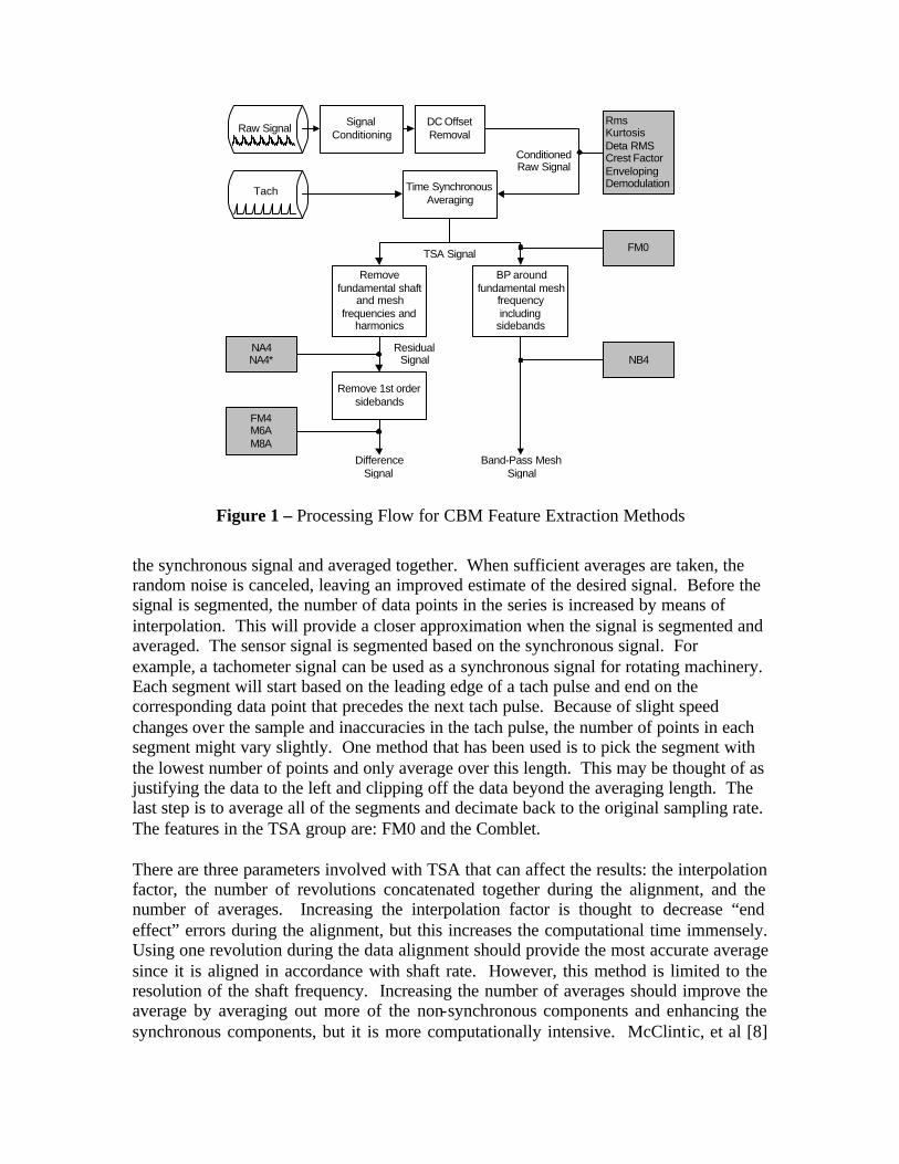
Before any feature can be calculated on the raw vibration data, the data must be conditioned or preprocessed. Conditioning may range from signal correction, based on the data acquisition unit and amplifiers used, and mean value removal to time-synchronous averaging and filtering. A variety of signal processing techniques are used based on the feature being implemented. This section will provide the necessary framework that is required for feature analysis. This paper focuses on thirteen traditional analysis features that are grouped into five different processing groups. The five processing groups are: 1) Raw signal (RAW), 2) Time synchronous averaged signal (TSA), 3) Residual signal (RES), 4) Difference signal (DIF), and 5) Band-pass mesh signal (BPM). These five groups along with the associa ted preprocessing and figures of merit are shown in Figure 1. The RAW preprocessing denotes features that are calculated from the raw or conditioned signal from the sensor. The only preprocessing needed for these features is conditioning the signal or removing the mean of the signal. Signal conditioning is simply multiplying all of the data points by some calibration constant that is based on the accelerometer and amplifier used. The features in this group are: RMS, Kurtosis, Delta RMS, Crest Factor, Enveloping and Demodulation. The TSA preprocessing entails time synchronous averaging of the raw data. Time synchronous averaging is a signal processing technique that is used to extract repetitive signals from additive noise. This process requires an accurate knowledge of the repetitive frequency of the desired signal or a signal that is synchronous with the desired signal. The raw data is then divided up into segments of equal length blocks related to

Raw Signal SignalConditioning

DC OffsetRemoval

RmsKurtosisDeta RMSCrest FactorEnvelopingDemodulationTime Synchronous

Averaging

FM0

Tach

Removefundamental shaft

and meshfrequencies and

harmonics

BP aroundfundamental mesh

frequencyincluding

sidebands

NB4

Remove 1st ordersidebands

NA4NA4*

FM4M6AM8A

ConditionedRaw Signal

DifferenceSignal

Band-Pass Mesh Signal

ResidualSignal

TSA Signal

Figure 1 – Processing Flow for CBM Feature Extraction Methods

the synchronous signal and averaged together. When sufficient averages are taken, the random noise is canceled, leaving an improved estimate of the desired signal. Before the signal is segmented, the number of data points in the series is increased by means of interpolation. This will provide a closer approximation when the signal is segmented and averaged. The sensor signal is segmented based on the synchronous signal. For example, a tachometer signal can be used as a synchronous signal for rotating machinery. Each segment will start based on the leading edge of a tach pulse and end on the corresponding data point that precedes the next tach pulse. Because of slight speed changes over the sample and inaccuracies in the tach pulse, the number of points in each segment might vary slightly. One method that has been used is to pick the segment with the lowest number of points and only average over this length. This may be thought of as justifying the data to the left and clipping off the data beyond the averaging length. The last step is to average all of the segments and decimate back to the original sampling rate. The features in the TSA group are: FM0 and the Comblet. There are three parameters involved with TSA that can affect the results: the interpolation factor, the number of revolutions concatenated together during the alignment, and the number of averages. Increasing the interpolation factor is thought to decrease “end effect” errors during the alignment, but this increases the computational time immensely. Using one revolution during the data alignment should provide the most accurate average since it is aligned in accordance with shaft rate. However, this method is limited to the resolution of the shaft frequency. Increasing the number of averages should improve the average by averaging out more of the non-synchronous components and enhancing the synchronous components, but it is more computationally intensive. McClintic, et al [8]

shows how these parameters affect the residual and difference analysis features when processed on Mechanical Diagnostics Test Bed (MDTB) data. A detailed description of the Applied Research Laboratory’s MDTB can be found in [9]. The RES preprocessing calculates the residual signal, which consists of the time synchronous averaged signal with the primary meshing and shaft components along with their harmonics removed. What is unclear from the literature is how many harmonics to remove for the primary mesh and shaft components. For a time synchronous averaged data over one revolution, this means that the smallest resolution in the frequency domain is the shaft frequency. Therefore, this would mean removing every point in the spectrum. What has shown to produce favorable results is to high pass the data about some frequency and only remove the meshing frequency and all harmonics. The cut-off frequency of the high pass filter will be system dependent, but it should lie somewhere between DC and the fundamental meshing frequency. Also, removal of five mesh harmonics has produced results very similar to the results produced by removing all the harmonics, but this may be system dependent. Features in the RES group are: NA4 and NA4*. The DIF preprocessing section calculates the difference signal by removing the regular meshing components from the time synchronous averaged signal. The regular meshing components consist of the shaft frequency and its harmonics, the primary meshing frequency and harmonics along with the first order sidebands. Since the residual signal is the result of removing the primary meshing and shaft frequencies and harmonics, the DIF processing section can consist of removing only the sidebands of the primary meshing frequencies from the RES signal. Assuming that a high-pass filter or a limited number of shaft frequency harmonics were removed, this will mean that only the sidebands of the meshing frequency and its harmonics need to be removed. For the case where time synchronous averaging is performed over one revolution, the sidebands will be one bin on either side of the meshing frequency. The features in the DIF group are: FM4, M6A, and M8A. The BPM preprocessing section is used for only one processing feature, NB4. In this section the TSA signal is band-pass filtered around the primary gear mesh frequency, including as many sidebands as possible. The Hilbert transform is then applied to the filtered signal to produce a complex time series. The real part is the band-passed signal and the imaginary part is the Hilbert transform of the signal. The envelope is the magnitude of this complex time signal and represents an estimate of the amplitude modulation present in the signal due to the sidebands [4]. The processing flowchart shown in Figure 1 shows thirteen-feature processing routines that may be used for gear fault detection. Some of the features produce more than one value or figures of merit (FOM) and there are several feature functions that can be calculated at different preprocessing stages. The Energy, Demodulation and Enveloping features are examples of such features that return multiple parameters, while features such as Kurtosis and RMS may be performed at different preprocessing levels. A brief overview of each feature is discussed in the following section.

Feature Extraction Technique Descriptions: RMS and Delta RMS The root mean square (RMS) value of a vibration signal is a time analysis feature that is the measure of the power content in the vibration signature. This feature is good to track the overall noise level, but it will not provide any information on which component is failing. It can be very effective in detecting a major out-of-balance in rotating systems. Below is the equation that is used to calculate the root mean square value of a data series, xn over length N.

∑=

=N

n

nxN

RMS1

2*1

(1)

Delta RMS is simply the difference between the current RMS value and the previous. Kurtosis Kurtosis is defined as the fourth moment of the distribution and measures the relative peakedness or flatness of a distribution as compared to a normal distribution. Kurtosis provides a measure of the size of the tails of distribution and is used as an indicator of major peaks in a set of data. As a gear wears and breaks this feature should signal an error due to the increased level of vibration [1]. The equation for kurtosis is given by:

221

4

)(*

])([

σµ

NnyN

nk∑ ==

− (2)

where y(n) is the raw time series at point n, µ is the mean of the data, σ2 is the variance of the data, and N is the total number of data points. Crest Factor The simplest approach to measuring defects in the time domain is using the RMS approach. However, the RMS level may not show appreciable changes in the early stages of gear and bearing damage. A better measure is to use “crest factor” which is defined as the ratio of the peak level of the input signal to the RMS level. Therefore, peaks in the time series signal will result in an increase in the crest factor value. For normal operations, crest factor may reach between 2 and 6. A value above 6 is usually associated with machinery problems. This feature is used to detect changes in the signal pattern due to impulsive vibration sources such as tooth breakage on a gear or a defect on the outer race of a bearing. The crest factor feature is not considered a very sensitive technique. Below is the equation for the crest factor:

RMSPeakLevel

FactorCrest = (3)

where PeakLevel is the peak level of the raw time series, and RMS is the root mean square of the raw data. Enveloping Enveloping is used to monitor the high-frequency response of the mechanical system to periodic impacts such as gear or bearing faults. An impulse is produced each time a loaded rolling element makes contact with a defect on another surface in the bearing or as

a faulty gear tooth makes contact with another tooth. This impulse has an extremely short duration compared to the interval between the pulses. The energy from the defect pulse will be distributed at a very low level over a wide range of frequencies. It is this wide distribution of energy that makes bearing defects so difficult to detect by conventional spectrum analysis when they are in the presence of vibrations from gears and other machine components. Fortunately, the impact usually excites a resonance in the system at a much higher frequency than the vibration generated by the other components. This structural energy is usually concentrated into a narrow band that is easier to detect than the widely distributed energy of the bearing defect frequencies. With tooth wear and breakage, the side band activity near critical frequencies such as the output shaft frequency is expected to increase. The entire spectrum contains very high periodic signals associated with the gear mesh frequencies.

The envelope or high frequency technique focuses on the structure resonance to determine the health of a gear or the type of failure in a bearing. This technique consists of processing structure resonance energy with an envelope detector. The structure resonance is obtained by band-pass filtering the data around the structure resonance frequency. The band-pass filtered signal is then processed by an envelope detector, which consists of a half-wave (or full-wave) rectifier and a peak-hold and smoothing section. A simple envelope detector processing flow diagram is shown in Figure 2.

Figure 2 – Simple Envelope Detector Scheme.

The center frequency of the band-pass filter should be selected to coincide with the structure resonance frequency being studied. The bandwidth of the filter should be at least double the highest characteristic defect frequency. This will ensure that the filter will pass the carrier frequency and at least one pair of modulation sidebands. In practice, the bandwidth should be somewhat greater to accommodate the first two pairs of modulation sidebands around the carrier frequency. The rectifier in the envelope detector turns the bipolar filtered signal into a unipolar waveform. The peak-hold smoothing section will then remove the carrier frequency by smoothing/filtering the fast transitions in the signal. The remaining signal will then consist of the defect frequencies. This feature produces several figures of merit for analysis use. The primary figure of merit is the peak frequency and amplitude in the power spectral density of the enveloped data. Other figures of merit include the RMS and kurtosis values of the filtering section and the standard deviation of the output from the rectification and smoothing block.

Envelope Detector

Band-PassFilter

Half-waveor

Full-waveRectifier

Peak-HoldSmoothing

AccelerometerData

Band-PassFilteredSignal

RectifiedSignal

EnvelopeDetected

Signal

The envelope technique has been widely used in numerous applications and has shown successful results in the early detection of bearing faults. Besides early detection, this process can help distinguish the actual cause of bearing failure by inspecting the actual bearing defect frequencies. Demodulation During a normal gear roll, one tooth is essentially pushing another without sliding. When the teeth wear, sliding occurs. The energy that went into pushing before will now go into pushing and sliding, thus resulting in a change of amplitude or amplitude modulation of the vibrations at the gear mesh frequency (GMF) and its harmonics. Demodulation processing identifies periodicity in modulation of the carrier. The carriers used in this processing were the GMF and 2*GMF. Demodulation techniques detect the amplitude modulation components induced by gear wear in the region of a single frequency, in this case the GMF or 2* GMF. This differs from enveloping which detects the combined effects over a range of frequencies. To implement the demodulation technique, the raw data is high-passed filtered at 85%*GMF and then low-passed filtered at 115%*GMF. The power spectral density of the filtered signal is searched to obtain the actual carrier frequency (GMF). The actual carrier is used to amplitude demodulate the filtered carrier signal. The power spectral density of the resulting signal is searched within +/- five percent of the output shaft frequency. The figures of merit extracted for this technique are the frequency of the peak and the magnitude squared amplitude. FM0 FM0 is a relatively simple method used to detect major changes in the meshing pattern. Major tooth faults typically result in an increase of the peak-to-peak signal levels, but do not change the meshing frequency. FM0 is defined as the peak-to-peak level of the TSA signal divided by the sum of the amplitude at the gear-mesh frequency and it’s corresponding harmonics. For heavy wear the peak-to-peak remains constant while the meshing frequency decreases, causing the FM0 parameter to jump up. Both the above situations will result in a large increase in the FM0 parameter. However FM0 is not a good indicator for minor tooth damage [1]. The equation for FM0 is:

∑=

=n

iifA

PPAFM

1

)(0 (4)

where PPA is the peak-to-peak amplitude of the time synchronous averaged waveform and A(fi) is the amplitude of the gear-mesh fundamental and harmonics in the frequency domain. NA4 NA4 was developed to detect the onset of damage and to continue to react to this damage as it spreads and increases in magnitude [2]. NA4 is determined by dividing the fourth statistical moment of the residual signal by the current run time averaged variance of the residual signal, raised to the second power. The equation for NA4 is

( )

( )2

1 1

2

1

4

14

−

−=

∑ ∑

∑

= =

=

m

j

N

ijij

N

ii

rrm

rrNNA

(5)

where r is the residual signal, r the mean value of the residual signal, N is the total number of data points in time record, and m is the current time record number in the run ensemble. NA4* NA4* (or ENA4) was developed as an enhanced version of NA4, and was expected to be more robust when progressive damage occurs [2]. This added robustness is incorporated into NA4* by normalizing the fourth statistical moment with the residual signal variance for a gearbox in good condition instead of the running variance, which is used for NA4. The equation for NA4* follows:

( )

( )2

2

1

4

~

1

*4M

rrNNA

N

ii∑

=−

= (6)

where r is the residual signal, r is the mean value of residual signal, N is the total number of data points in time record, and 2

~M is the variance of the residual signal for a gearbox in good condition. FM4 FM4 was developed to detect changes in the vibration pattern resulting from damage on a limited number of gear teeth [2]. FM4 is calculated by applying the fourth normalized statistical moment to this difference signal as given in the equation:

( )

( )2

1

2

1

4

4

−

−=

∑

∑

=

=

N

ii

N

ii

dd

ddNFM (7)

where d is the difference signal, d is the mean value of difference signal, and N is the total number of data points in the time record. A difference signal from a gear in good condition will be primarily Gaussian noise therefore resulting in a normalized kurtosis value of 3. As a defect develops in a tooth, peaks will grow in the difference signal that will result in the kurtosis value to increase beyond 3. M6A and M8A M6A and M8A were proposed by Martin [6] to detect surface damage on machinery components. Both of these features are applied to the difference signal. The theory behind M6A and M8A is the same as that for FM4, except that M6A and M8A are expected to be more sensitive to peaks in the difference signal. The equations for M6A and M8A are as follows:

( )

( )3

1

2

1

62

6

−

−=

∑

∑

=

=

N

ii

N

ii

dd

ddNAM

( )

( )4

1

2

1

83

8

−

−=

∑

∑

=

=

N

ii

N

ii

dd

ddNAM (8)

where d is the difference signal, d is the mean value of difference signal, and N is the total number of data points in time record. NB4 NB4 is similar to NA4 except that instead of using the residual signal, NB4 uses the envelope of a band-passed segment of the time synchronous averaged signal. The idea behind this method is that a few damaged gear teeth will cause transient load fluctuations that are different from the normal tooth load fluctuations. The theory suggests that these fluctuations will be manifested in the envelope of a signal which is band-pass filtered about the dominant meshing frequency. The dominant meshing frequency is either the primary meshing frequency or one of its harmonics whichever appears to give the most robust group of sidebands [5]. Some suggest that the width of the band-pass filter depends on the location of the meshing frequency to other meshing frequency harmonics, while others suggest using a bandwidth giving the maximum amount of sidebands even if the sidebands interfere with those from other harmonics [5]. The reasoning of the latter method is to assume that the interference from other sidebands is negligible and includes as many of the primary modulating sidebands as plausible. The envelope of the band-passed signal is the magnitude of the complex (i.e., analytic) signal obtained by applying the Hilbert transform to the band-passed signal:

( ) ( )[ ]22)()( tAHtAtE += (9)

where E(t) is the envelope of the band-passed signal, A(t) is the band-passed signal, and H[A(t)] is the Hilbert transform of the band-passed signal [4]. The analytic signal is A(t)+iH[A(t)]. NB4 is then determined by dividing the fourth statistical moment of this envelope signal by the current run time averaged variance of the envelope signal, raised to the second power, with the equation following:

( )

( )2

1 1

2

1

4

14

−

−=

∑ ∑

∑

= =

=

m

j

N

ijij

N

ii

EEm

EENNB (10)

where E is the envelope of the band-passed signal, E is the mean value of envelope signal, N is the total number of data points in time record, and m is the current time record number in the run ensemble.

Penn State ARL CBM Toolbox: The CBM toolbox is a conglomeration of all the traditional features discussed in this paper along with a few non-traditional features, such as the wavelet transform, Interstitial and Comblet. This toolbox was developed in Matlab to provide a researcher with a set of standard processing routines for machinery prognostics. The flexibility of the toolbox allows the user to easily add features and input/output data file formats. By using an INI file interface, the user can easily change analysis parameters and process data with one Matlab command. Or the user may pass data directly into any of the individual feature routine. The INI file is a text file format that stores parameters and information about the Accelerometers, signal conditioning, preprocessing parameters and the feature parameters. The flowchart in Figure 3 shows the data flow into and out of the CBM toolbox. To ensure that there are no issues on how the data was processed, all of the parameters and information stored in the INI file is placed in the output data file along with the feature data.

Figure 3 – Inputs and Output of the CBM Toolbox.

The CBM toolbox currently has 19 built- in features that provide 40 figures of merit. The specific features and figures of merit of the toolbox are shown in Table 1. All of the analysis features and input/output data files are controlled via a single command line to make batch processing a breeze.

Table 1 - Features and Figures of Merit of the CBM Toolbox

Raw Data

INI File

Gearbox FOMToolkit

Output Data File:

RequestedFeatures

� HealthMatrix� Process Names� INI Settings

Normally features are compared on a linear scale plot for their diagnostic and prognostic ability. However, when the number of features increases, it is difficult to obtain a “quick look” yet comprehensive comparison in this manner. Figure 4 is an alternative way to view the features. The x-labels are the feature names, the y-labels are the time in hours of the data (which increase from top to bottom), and each colored rectangle represents the normalized feature value for that snapshot. By viewing the features in this manner, correlation across features can more easily be seen as well as significant changes within a feature. It is important to consider relative changes within a feature opposed to actual feature values since they can easily vary due to environmental affects. Prognostic features can also be picked out in this manner by noticing gradual and increasing value changes. The salient features found in the image, can then be plotted on a linear scale for more in depth analysis.

Figure 4 - Figure of Merit Map

Conclusions: While there are many ways to process vibration data for CBM purposes, the details in the preprocessing steps must be standardized in order to facilitate reliable and repeatable assessments. Commonly used terms in the CBM community and specific preprocessing requirements needed for the given feature analysis was discussed. This paper listed some of the most traditional features used for machinery diagnostics and prognostics and presented some of the signal processing parameters that impact their sensitivity. In order to advance in the knowledge base and evaluate the performance of such diagnostic and prognostic features for damage assessment and tracking, the research community needs to understand and document these processing details and sensitivities.

Acknowledgements: This work was supported by the Office of Naval Research through the Multidisciplinary University Research Initiative for Integrated Predictive Diagnostics (Grant Number N00014-95-1-0461), an Accelerated Capabilities Initiative in Human Information Management (N00014-98-C-0066) through a subcontract by CHI Systems, Inc. (CHI-9803-002), and an Accelerated Capabilities Initiative for Condition-Based Maintenance (N00014-96-1-1147). The content of the information does not necessarily reflect the position or policy of the Government, and no official endorsement should be inferred. The authors would like to acknowledge Mike Van Dyke for his guidance. References: 1. Zakrajsek, James J., NASA Technical Memorandum 102340, Lewis Research Center,

Cleveland, Ohio, 2. Zakrajsek, J. J., Townsend, D. P., Decker, H. J., An Analysis of Gear Fault Detection

Methods as Applied to Pitting Fatigue Failure Data, The Systems Engineering Approach to Mechanical Failure Prevention, 47th Meeting of the MFPG, 1993.

3. Johnson, R. A., Miller and Freund’s Probability and Statistics for Engineers, Fifth Edition, Prentice- Hall, Inc., Englewood Cliffs, NJ, 1994.

4. Zakrajsek, J. J., Handschuh, R. F., Lewicki, D. G., and Decker, H. J., Detecting Gear Tooth Fracture in a High Contact Ratio Face Gear Mesh, Proceedings of the 49th Meeting of the Mechanical Failure Prevention Group, Virginia Beach, VA, April 18-20, 1995.

5. Zakrajsek, J. J., An Investigation of Gear Mesh Failure Prediction Techniques, NASA Technical Memorandum 102340 (89-C-005), November 1989.

6. Martin, H. R., Statistical Moment Analysis As a Means of Surface Damage Detection, Proceedings of the 7th International Modal Analysis Conference, Society for Experimental Mechanics, Schenectady, NY, 1989, pp. 1016-1021.

7. Maynard, Kenneth P., Interstitial Processing: The Application of Noise Processing to Gear Fault Detection, International Conference on Condition Monitoring, University of Wales Swansea, April 12-15, 1999, p. 77-86

8. McClintic, K., Lebold, M., Maynard, K., Byington, C., Campbell, R., Residual and Difference Feature Analysis with Transitional Gearbox Data, 54th Meeting of the MFPT, Virginia, May 2000.

9. Byington, C.S., Kozlowski, J.D., Transitional Data for Estimation of Gearbox Remaining Useful Life, 51st Meeting of the Society for Machinery Failure Prevention Technology (MFPT), April 1997.