Review of Soil Erosion Assessment using RUSLE Model and GIS

Journal of Biology, Agriculture and Healthcare www.iiste.org

ISSN 2224-3208 (Paper) ISSN 2225-093X (Online)

Vol.5, No.9, 2015

36

Review of Soil Erosion Assessment using RUSLE Model and GIS

B.G. Jahun1*

R. Ibrahim1 N.S. Dlamini

1 S. M. Musa

2

1.Faculty of Engineering, Department of Biological and Agricultural Engineering, Universiti Putra Malaysia,

Serdang, Selangor Darul Ehsan 43400, Malaysia

2.Faculty of Engineering, Department of Agricultural and Bioresource Engineering, Abubakar Tafawa Balewa

University Bauchi PMB 0248 Bauchi State, Nigeria

Email address of the corresponding Author:bgjahu.com

Abstract

Soil erosion is one of the world environmental problems the world is facing in the 21st century affecting human

society and is listed amongst the top environmental issues facing the world including increasing human

population, water shortages, loss of biodiversity, energy and human diseases. An estimated 10 million hectares

of agricultural lands are degraded and turned into un-farmable areas due to soil erosion thus resulting in reduced

food production for the 3.7 billion malnourished people as reported by World Health Organization. Estimation of

soil erosion loss and evaluation of soil erosion risk has become an urgent task by many nations before

implementing soil conservation practices. There is now a large published literature on the application of the

Revised Universal Soil Loss Equation known as the RUSLE model in combination with GIS technology for

predicting soil loss and erosion risks in different regions. This review paper assesses the current literature on the

combined application of RUSLE and GIS, examining new developments in deriving the five RUSLE

components. The literature review shows that using the traditional RUSLE model in mapping out soil erosion in

large watersheds poses challenges. The combined effect of RUSLE and GIS provides a useful and efficient tool

for predicting long-term soil erosion potential and assessing soil erosion impacts. However, there is a need to

further investigate better ways of deriving the conservation and management factor (P) in the RUSLE for better

on future studies. Data source and quality is also another key issue in GIS application, thus great care must be

given in checking and pre-processing GIS data, including conversion to different formats, geo-referencing, data

interpolation and registration. Finally, validation of the soil erosion loss using reference data is also a valuable

input towards improving the quality and correctness of the results.

Keywords: Soil erosion, RUSLE, watershed, GIS

1. Introduction

Soil erosion is define as a process in which topsoil on the soil surface is carry away from the land by water or

wind and transported to other surfaces. It is considered the second prevalent environmental problem the world

faces after population growth. Pimentel et al., (2009) revealed shocking figures about the erosion phenomenon,

that is, most of the soil from farmlands is washed away about 10–40 times faster than it is being replaced, citing

examples that United States was losing soil 10 times faster than the regular replacement rate, China and India are

said to be losing soil 30–40 times faster. Soil erosion trend has increased throughout the 20th

century. The land

degradation in the world is about 85% which is associated with soil erosion, most of which occurred since the

end of World War II, causing a 17% reduction in crop productivity (Angima et al., 2003).

The extent of soil erosion shows that it’s a worldwide environmental problem with some areas such as

Southern Europe and the Mediterranean region being extremely prone to erosion due to prolonged dry periods

and heavy erosive rainfall, falling on steep slopes with fragile soils, causing in considerable amounts of erosion

(Onori et al., 2006). Mitasovaet al., (1996) reported that in Greece, soil erosion affects 3.5 million hectares

(26.5%) of the country’s total land area. In countries like Malaysia, heavy rainfall is a frequent occurrence which

causes soil erosion and landslides especially in steep areas where massive development occurs due to heavy

pressure from agricultural and urban development (Khosrokhani and Pradhan, 2013; Pradhan et al., 2012).

Himalayas in Southeast Asia and the Andes in South America, suffer some of the world’s highest erosion rates

because of the mountainous regions (Ismail and Ravichandran, 2008).

Literature has shown that eroded soils transport pesticides, nutrients, and other harmful farm chemicals

into streams, rivers, pollute surface and groundwater resources (Gallaher and Hawf, 1997), reduce productivity

and crop yields (Renard et al.,1997), caused air pollution through emissions of gases such as carbon dioxide

(CO2), methane (CH4), and nitrous oxide (N2O) (Cox and Madramootoo, 1998). Due to erosion over the past 40

years, 30% of the world’s arable land has become unproductive. The erosion occurs when soil is left exposed to

rain or wind energy thereby raindrops hit the exposed soil with great energy and easily displace the soil particles

from the surface. Soil erosion has three-stage process involving detachment, transport and deposition as

mentioned by Merritt et al., (2003). The impact intensified on sloping land, where often more than half of the

surface soil is carried away as the water splashes downhill into valleys and waterways. The rate of erosion is thus

influenced by the soil composition, slope of the land, and extends of vegetative cover.



Vol.5, No.9, 2015

37

Thus, timely and accurate estimation of soil erosion loss or evaluation of risk has become imperative

for many countries. It is also useful to make estimate of how fast the soil is being eroded before affecting any

conservation strategies. Due to the nature of the erosion process, erosion control requires a quantifiable and

qualitative evaluation of potential soil erosion on a specific site, and the knowledge of terrain, cropping system,

soils, and management practices. Many researchers involved in soil erosion research for quiet long time, and

effort was put in understanding the mechanism of soil erosion, predicting the rate of soil erosion and soil loss

both at catchment scale or plot (Fu et al., 2004; Fu et al., 2005; Kang et al., 2001), and at a regional scale.

Several sediment transport and soil erosion models have been developed around the world to estimate rates of

sediment and nutrient transport under different land use systems. There are three categories of model: the

empirical models, the conceptual models and physically-based models as suggested by Merritt et al., (2003).

These include the USLE and GIS based USLE, WEPP, AGNPS, LISEM and EUROSEM models. These models,

however, vary significantly in their complexity, inputs and requirements, the processes represent and the manner

in which these processes are represented, the scale of intended use and the types of output information they

provide (Ismail and Ravichandran, 2008; Merritt et al., 2003).

Universal Soil Loss Equation (USLE) has emerges as a leading model and has been broadly used both

in United States and all over the world in both agricultural and hilly watersheds owing to its simplicity of

obtaining parameters (Wilson and Lorang, 1999). This model was first developed by Wischmeier and Smith

(1978) and collected soil erosion data in 21 States in United States, analyzed and assessed various dominating

factors of soil erosion, and introduced USLE to assess soil erosion by water. The USLE predicts the long-term

average and annual rate of erosion on a field slope based on rainfall pattern, soil type, topography, crop system,

and management practices (Kouli et al., 2009). For many decades now, comprehensive research on soil erosion

by water has been conducted using this model. The model was then improved and replaced by the revised

version now known as Revised Universal Soil Loss Equation (RUSLE) by additional data and incorporating

recent research results to further enhance its ability to predict water erosion by integrating information made

available through research of the past 40 years Renard et al., (1997). RUSLE is still widely used, as some of the

models such as the WEPP are difficult to use for most users. In addition, the combination of remote sensing and

GIS techniques with soil erosion models, such as RUSLE, proved to be an effective approach for estimating the

magnitude and spatial distribution of erosion by other researchers. GIS is a tool efficient to integrate various

datasets and assess dynamic system such as soil erosion.

The aim is to review the current state of erosion assessment and GIS applications in the literature. This

will include; 1) the traditional application of the RUSLE model in assessing erosion, 2) and the application of

GIS and remote sensing techniques in predicting and estimating the magnitude and spatial distribution of erosion

at catchment or regional scales using RUSLE.

2. Traditional Methods of Soil Erosion Loss using RULSE

The historical background of erosion-prediction technology started with analyses as reported by Renard et al.,

(1997) to find the major variables that affect soil erosion by water. They listed three major factors: potential

erosivity of rainfall and runoff, susceptibility of soil to erosion, and soil protection done by plant cover. Zingg

(1940) published the first equation for calculating field soil loss as reported by Moore and Burch, (1986). They

described mathematically the effects of slope steepness and slope length on erosion. Smith (1976) also gives

additional factors for support practices and cropping system to the equation. The concept of specific annual soil-

loss limit and the resulting equation to develop a graphic method for selecting conservation practices for certain

soil conditions in the Midwestern United States were added.

Browning and associates (1947) as reported by Renard et al., (1997) added soil erodibility and

management factors to the Smith equation and prepared extensive tables of relative factor values for different

soils, crop rotations, and slope lengths. The approach emphasized the evaluation of slope-length limits for

different cropping systems on specific soils and slope steepness with and without, terracing, contouring, or strip-

cropping. Moore and Burch, (1986) reported a method for estimating soil losses from fields of clay pan soils.

Soil-loss ratios at different slopes were given for contour farming, strip-cropping, and terracing. The

recommended limits for slope length were presented for contour farming. Also, the equation is of limited value

since it cannot provide information on the fate of sediment once it is eroded. The USLE model is not able to

predict deposition or the pathways taken by eroded material and sediments as it moves from hill slope sites to

water bodies. In European context, the most important consequences of erosion are pollution and sedimentation

downstream rather than loss of productivity on-site. Policy-makers need to know more about the location of

sediment sources and sinks. Similarly, the design of strategies to control pollution associated with erosion runoff

and on agricultural land requires knowledge of what happens in individual rainstorms, seldom on a minute-by-

minute basis, in order to forecast the size and timing of peak discharges of water and sediment from hill slopes to

rivers. The USLE cannot provide this because it predicts only mean annual soil loss. The need for an alternative

approach was recognized by improving on the USLE.



Vol.5, No.9, 2015

38

3. Application of GIS techniques for facilitating erosion estimation

Traditionally, the RUSLE model was developed to assess soil erosion risk for small local-scale watersheds.

However, with the spatial widespread occurrence and acceleration of the soil erosion process and water quality

problems, the use of RUSLE model poses inherent drawback with respect to costs of applying it,

representativeness of site, and on reliability of predicted results (Lu., 2004; Wilson and Lorang, 1999). Thus,

mapping of soil erosion spatial distribution is often problematic with the traditional RUSLE model (Lu et al.,

2004).

The advent of GIS technology stimulated an explosive increase in GIS based models applications on

regional scale. The combination of GIS technology with erosion models such as the RUSLE has improved the

efficiency for estimating spatial distribution and magnitude of erosion risk with reasonable costs and better

accuracy as documented by several researchers in the literature (Dziewonski et al., 1975; Mitasova et al., 1996;

Cox and Madramootoo, 1998; Molnár and Julien, 1998; Millward and Mersey, 1999; Wilson and Lorang, 1999;

Yitayew, 1999; Gibbs et al., 2003; Lewis et al et al., 2005; Fu et al., 2006; Erdogan et al., 2007; Neshat et al.,

2014).

3.1. General methods for estimating RUSLE factors in a GIS environment.

The application of RUSLE in a GIS framework has been employed in various circumstances such as

mountainous tropical watersheds, large scale watersheds, in agricultural dominant watersheds, in areas with

distinct wet and dry seasons, and also in areas with dynamic changes such as in land cover patterns, agricultural

farmlands and developments. The RUSLE model consists of three main databases: 1) Climatic and survey

database which contains information such as monthly temperature and precipitation and contours that is required

for the calculating the erosivity factor as well as slope length and steepness factors (LS). 2) Crop database

contains information necessary for determining the surface cover factor (C). 3) The soil data contains soil survey

and soil characterization data which is responsible determining the soil erodibility factor (K).

RUSLE model calculates the average annual soil erosion loss by considering the five factors as defined

in equation 1 (Renard et al., 1997). Based on the plethora of literature, the general methodology of applying the

RUSLE is to estimate each of the factors in the model. Several techniques for estimating these factors have been

developed by previous researchers ranging from use of climate data, soil and geological maps, remotely sensed

satellite images, empirical formulas and digital elevation model (DEM) obtained from various sources. The

techniques used to generate the model factors and the results obtained are described in the next sections of this

article.

A = RKLSCP 1)

Where; A = predictedlong − termaverageofannualsheetandrillsoilloss, tha !yr !

R = rainfall − runofferosivityfactor,MJmmha !h !yr !

K = soilerosivityfactor,MghMJ !mm !

L = slopelength,m

S = slopesteepness,%

C = coverandmanagementfactor P = supportpractice

3.1.1. The rainfall erosivity factor (R) Rainfall erosivity is the potential ability of rain to cause soil erosion (Lal, 1990). R factor is the most important

parameter in erosion estimation by RUSLE as suggested by several researchers and its correlation with soil loss

is high in many region and world rainfall site stations Fu et al., 2006; Millward and Mersey, 1999; Renard and

Freimund, 1994; Wischmeier and Smith, 1978).

The general procedure employed by researchers in determining the erosion factor involves using

observed historical rainfall data as well as application of several different formulas depending on the prevailing

conditions of the area. The estimation of R factor poses a challenge in data poor areas or in situations where

climate stations are extremely sparse. Fu et al., (2006) developed an equivalent R factor (R'() for the Inland

Pacific Northwest (IPNW) region in the USA by relating the R factor linearly with the local annual precipitation P*, mm as shown in equation 2.

R'( = −823.8 + 5.21P* 2)

Where;

R'( = EquivalentRfactorforuniqueclimaticcondition

P* = annualprecipitation,mm



Vol.5, No.9, 2015

39

Millward and Mersey, (1999) also faced similar conditions of sparse climate data when assessing

erosion risk in a particular watershed in Mexico. They employed a rather more improved technique in generating

rainfall data. They used remote rainfall stations and rainfall was interpolated from the remote stations using

interpolation methods such as kriging and inverse distance. Interpolation was done in IDRISI using an algorithm

INTERPOL and the R factor was then estimated using the EI30 measurement. The technique used improved the

results of their analysis. The simplest technique is the one used by Yitayew et al., (1999) where they converted

on-site rain gauge data to energy intensity (EI) values and multiplying it by the maximum 30-min rainfall

intensity expressed as I30.

Renard and Freimund (1994) propose using the monthly and mean annual rainfall in environments with

available long-term rainfall data, in the modified Fournier index, F, previously introduced by Sauerborn et al.,

(1999) which is defined by equation 3.

F = ∑ 6789!:;<! 3)

Where; F = ModifiedFournierindex

P = meanannualrainfalldepth,mm

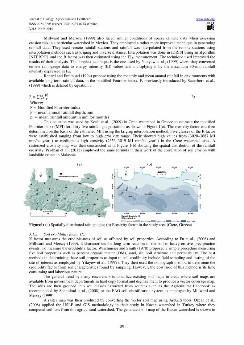
p; = meanrainfallamountinmmformonthi This equation was used by Kouli et al., (2009) in Crete watershed in Greece to estimate the modified

Fournier index (MFI) for thirty five rainfall gauge stations as shown in Figure 1(a). The erosivity factor was then

determined on the basis of the estimated MFI using the kriging interpolation method. Five classes of the R factor

were established ranging from low to high erosivity range. Their showed high values from (3020–3687 MJ

mm/ha year-1

) to medium to high erosivity (2353–3019 MJ mm/ha year-1

) in the Crete watershed area. A

rasterized erosivity map was then constructed as in Figure 1(b) showing the spatial distribution of the rainfall

erosivity. Pradhan et al., (2012) employed the same formula in their work of the correlation of soil erosion with

landslide events in Malaysia.

(a) (b)

Figure1: (a) Spatially distributed rain-gauges; (b) Erosivity factor in the study area (Crete, Greece)

3.1.2. Soil erodibility factor (K) K factor measures the erodible-ness of soil as affected by soil properties. According to Fu et al., (2006) and

Millward and Mersey (1999), it characterizes the long term reaction of the soil to heavy erosive precipitation

events. To measure the erodibility factor, Wischmeier and Smith (1978) proposed a simple procedure measuring

five soil properties such as percent organic matter (OM), sand, silt, soil structure and permeability. The best

methods in determining these soil properties as input to soil erodibility include field sampling and testing of the

site of interest as employed by Yitayew et al., (1999). They then used the nomograph method to determine the

erodibility factor from soil characteristics found by sampling. However, the downside of this method is its time

consuming and laborious nature.

The general trend by many researchers is to utilize existing soil maps in areas where soil maps are

available from government departments in hard copy format and digitize them to produce a vector coverage map.

The soils are then grouped into soil classes extracted from sources such as the Agricultural Handbook as

recommended by Shamshad et al., (2008) or the FAO soil classification system as employed by Millward and

Mersey (1999).

A raster map was then produced by converting the vector soil map using ArcGIS tools. Ozcan et al.,

(2008) applied the USLE and GIS methodology in their study in Kazan watershed in Turkey where they

computed soil loss from this agricultural watershed. The generated soil map of the Kazan watershed is shown in



Vol.5, No.9, 2015

40

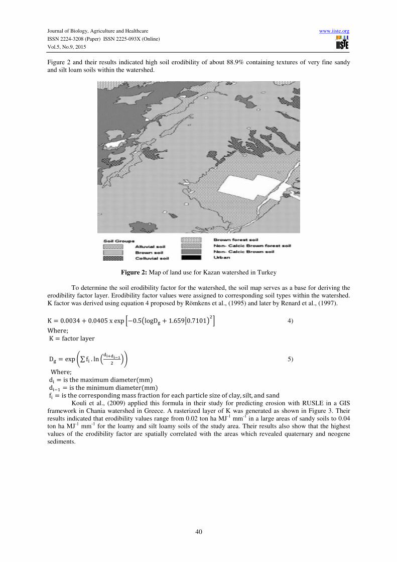
Figure 2 and their results indicated high soil erodibility of about 88.9% containing textures of very fine sandy

and silt loam soils within the watershed.

Figure 2: Map of land use for Kazan watershed in Turkey

To determine the soil erodibility factor for the watershed, the soil map serves as a base for deriving the

erodibility factor layer. Erodibility factor values were assigned to corresponding soil types within the watershed.

K factor was derived using equation 4 proposed by Römkens et al., (1995) and later by Renard et al., (1997).

K = 0.0034 + 0.0405xexp @−0.5AlogDC + 1.659F0.7101H:I 4)

Where;

K = factorlayer

DC = exp J∑ f; . ln KL7MN7OP: QR 5)

Where; d; = isthemaximumdiameter(mm) d; ! = istheminimumdiameter(mm) f; = isthecorrespondingmassfractionforeachparticlesizeofclay, silt, andsand

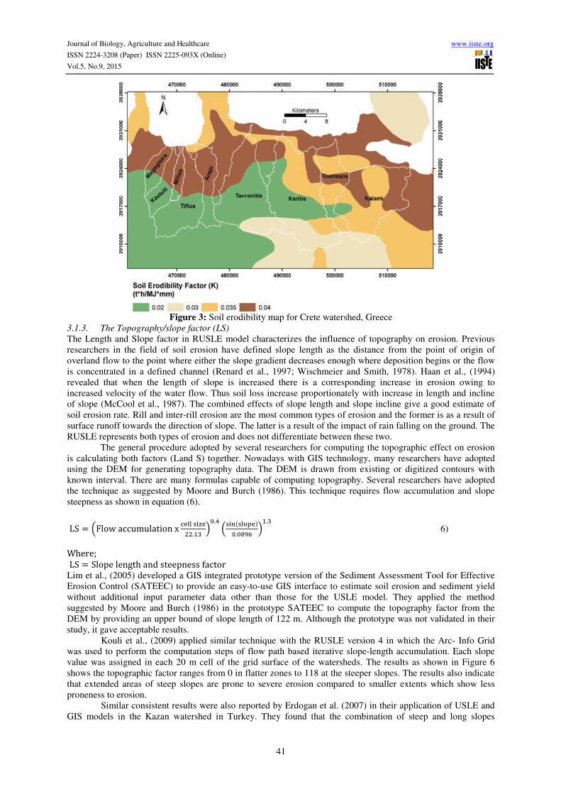
Kouli et al., (2009) applied this formula in their study for predicting erosion with RUSLE in a GIS

framework in Chania watershed in Greece. A rasterized layer of K was generated as shown in Figure 3. Their

results indicated that erodibility values range from 0.02 ton ha MJ-1

mm-1

in a large areas of sandy soils to 0.04

ton ha MJ-1

mm-1

for the loamy and silt loamy soils of the study area. Their results also show that the highest

values of the erodibility factor are spatially correlated with the areas which revealed quaternary and neogene

sediments.



Vol.5, No.9, 2015

41

Figure 3: Soil erodibility map for Crete watershed, Greece

3.1.3. The Topography/slope factor (LS) The Length and Slope factor in RUSLE model characterizes the influence of topography on erosion. Previous

researchers in the field of soil erosion have defined slope length as the distance from the point of origin of

overland flow to the point where either the slope gradient decreases enough where deposition begins or the flow

is concentrated in a defined channel (Renard et al., 1997; Wischmeier and Smith, 1978). Haan et al., (1994)

revealed that when the length of slope is increased there is a corresponding increase in erosion owing to

increased velocity of the water flow. Thus soil loss increase proportionately with increase in length and incline

of slope (McCool et al., 1987). The combined effects of slope length and slope incline give a good estimate of

soil erosion rate. Rill and inter-rill erosion are the most common types of erosion and the former is as a result of

surface runoff towards the direction of slope. The latter is a result of the impact of rain falling on the ground. The

RUSLE represents both types of erosion and does not differentiate between these two.

The general procedure adopted by several researchers for computing the topographic effect on erosion

is calculating both factors (Land S) together. Nowadays with GIS technology, many researchers have adopted

using the DEM for generating topography data. The DEM is drawn from existing or digitized contours with

known interval. There are many formulas capable of computing topography. Several researchers have adopted

the technique as suggested by Moore and Burch (1986). This technique requires flow accumulation and slope

steepness as shown in equation (6).

LS = KFlowaccumulationx U'VVW;X'::.!Y QZ.[ KW;\(WV]6')Z.Z^_` Q

!.Y 6)

Where;

LS = Slopelengthandsteepnessfactor Lim et al., (2005) developed a GIS integrated prototype version of the Sediment Assessment Tool for Effective

Erosion Control (SATEEC) to provide an easy-to-use GIS interface to estimate soil erosion and sediment yield

without additional input parameter data other than those for the USLE model. They applied the method

suggested by Moore and Burch (1986) in the prototype SATEEC to compute the topography factor from the

DEM by providing an upper bound of slope length of 122 m. Although the prototype was not validated in their

study, it gave acceptable results.

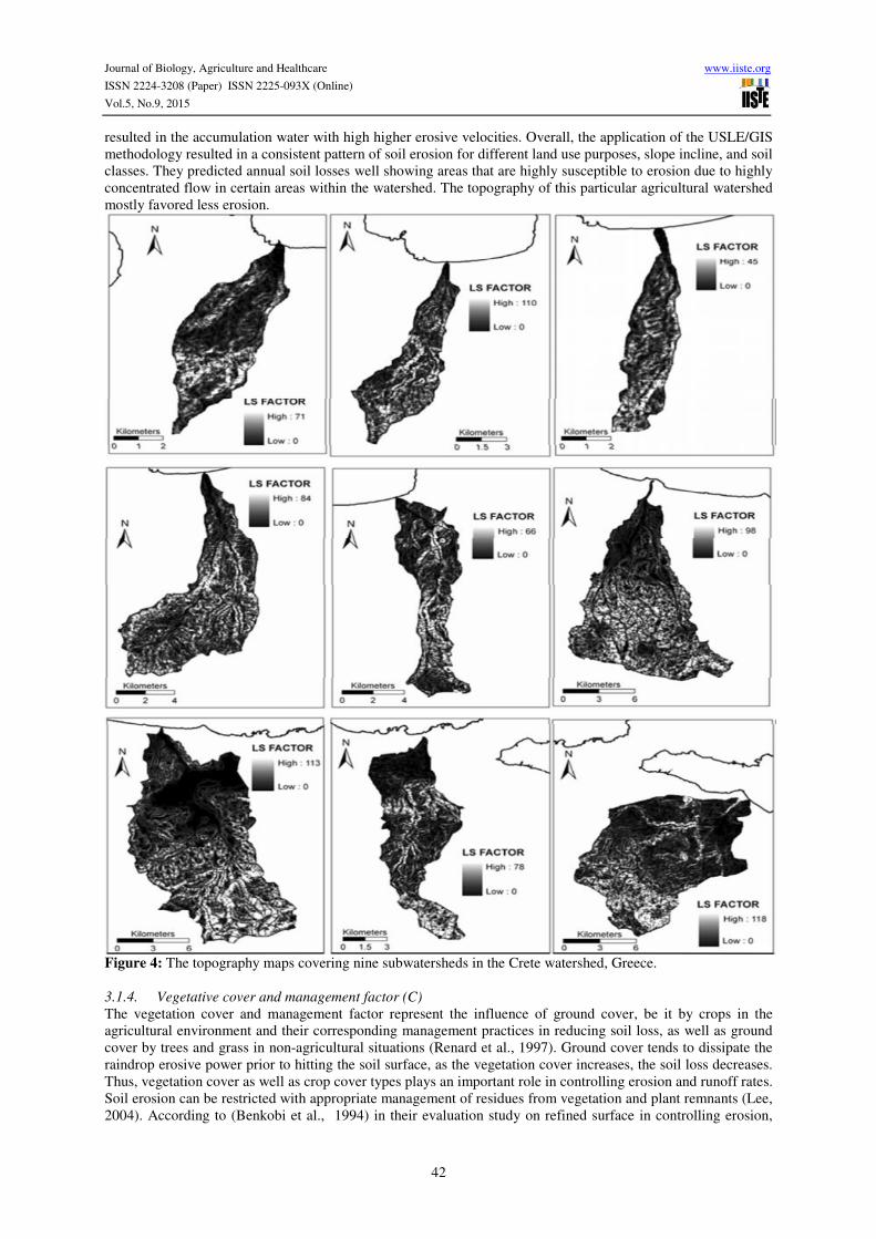
Kouli et al., (2009) applied similar technique with the RUSLE version 4 in which the Arc- Info Grid

was used to perform the computation steps of flow path based iterative slope-length accumulation. Each slope

value was assigned in each 20 m cell of the grid surface of the watersheds. The results as shown in Figure 6

shows the topographic factor ranges from 0 in flatter zones to 118 at the steeper slopes. The results also indicate

that extended areas of steep slopes are prone to severe erosion compared to smaller extents which show less

proneness to erosion.

Similar consistent results were also reported by Erdogan et al. (2007) in their application of USLE and

GIS models in the Kazan watershed in Turkey. They found that the combination of steep and long slopes



Vol.5, No.9, 2015

42

resulted in the accumulation water with high higher erosive velocities. Overall, the application of the USLE/GIS

methodology resulted in a consistent pattern of soil erosion for different land use purposes, slope incline, and soil

classes. They predicted annual soil losses well showing areas that are highly susceptible to erosion due to highly

concentrated flow in certain areas within the watershed. The topography of this particular agricultural watershed

mostly favored less erosion.

Figure 4: The topography maps covering nine subwatersheds in the Crete watershed, Greece.

3.1.4. Vegetative cover and management factor (C) The vegetation cover and management factor represent the influence of ground cover, be it by crops in the

agricultural environment and their corresponding management practices in reducing soil loss, as well as ground

cover by trees and grass in non-agricultural situations (Renard et al., 1997). Ground cover tends to dissipate the

raindrop erosive power prior to hitting the soil surface, as the vegetation cover increases, the soil loss decreases.

Thus, vegetation cover as well as crop cover types plays an important role in controlling erosion and runoff rates.

Soil erosion can be restricted with appropriate management of residues from vegetation and plant remnants (Lee,

2004). According to (Benkobi et al., 1994) in their evaluation study on refined surface in controlling erosion,



Vol.5, No.9, 2015

43

noted that the surface cover and slope length and steepness are crucial in controlling soil loss.

Traditionally, the surface cover factor is derived using empirical equations based on the measurements

of many variables related to ground covers collected in the sample plots. It can also be derived from weighted

average soil loss ratios (SLRs) that are determined from a series of sub-factors that include prior land-use,

canopy cover, surface cover and surface roughness (Renard et al., 1991). Knowledge of these sub-factors can be

obtained from various sources including site visits. However, a quick and easier technique for determining the C

factor is estimating a constant cover management value. A cover management factor of 0.0013 was estimated by

(Yitayew et al., 1999) in their study in which they used GIS technique for facilitating erosion estimation in the

Walnut Gulch experimental watershed in Arizona, although they highlighted that caution should be used in

applying this technique.

However, the most widely used technique nowadays for deriving the surface cover factor is by

employing remote sensing techniques in producing land use/cover classification from satellite. Lu et al., (2004)

in their study of mapping soil erosion risk in the Brazilian Amazonia based their estimation of the surface cover

on the fraction images from spectral mixture analysis (SMA) of Landsat ETM+ image. By using equation 7, the

C factor was estimated on the assumption that abundant vegetation cover results in less soil loss and the

corresponding higher losses are as a result of less vegetation cover. However, they caution that in the process of

developing the C factor, there remains the need to calibrate obtained results using local (reference) data as

surface characteristics is captured at the time of image acquisition.

C = abc7d!eafgeabhiNjeafgkabhiNj 7)

Where; C = VegetativecoverandManagementfactor fW];V, fCmandfWnoL' = valuesofsoil, greevegetation, andshadeendmembers

The three fraction values of soil, green vegetation, and shade endmembers. The values

offW];V, fCm, fWnoL' parameters range from 0 to 1 and their sum equals 1.

The most commonly used remote sensing technique is the Normalized Difference Vegetation Index

(NDVI) for deriving the C factor. This index indicates the energy reflected by the earth for various conditions of

surface cover type and is derived from the equation (8) for LandSat-ETM. NDVI values have two bands ranging

between -1.0 to +1.0. When the measured spectral response of the earth surface is very similar to both bands, the

NDVI values will approach zero. A large difference between the two bands results in NDVI values at the

extremes of the data range (Kouli et al., 2009).

Vegetation that is actively growing represent a high reflectance in the Infrared portion of the spectrum

(Band 4, Landsat TM), compared with the visible portion (red, Band 3, Landsat TM), thus the NDVI values for

actively growing vegetation is positive. NDVI values for low vegetative surface cover range between -0.1 and

+0.1, while clouds and water bodies show a negative or zero values (Kouli et al., 2009).

8) Where; NDVI = NormalizedDifferenceVegetationIndex

Kouli et al., (2009) used the NDVI technique to obtain the C factor in their soil erosion prediction study

in Greece. The C factor surface was derived from the NDVI values using equation (7) as suggested by (Van der

Knijff et al., 2000). Their results looked realistic showing that forest areas had the C values nearing 0 while for

rocky terrain approaching 1. They also showed that the predicted slope values for the arable land are affected by

crop type and management practices.

C = e( s(K tuvwxOtuvwQ) 9)

Where; αandβareunitlessparametersthatdeterminetheshapeofthecurve

relatingtoNDVIandCfactor Recent work by Pradhan et al., (2012) also applied the remote sensing technique in their work on

erosion and landslide study in Malaysia. They used SPOT 5 images of 2005 and 2010 with 10m spatial

resolution to derive the C factor from a land cover map. The slope map was produced by assigning slope values

to different classes as shown in Figure 5. Although their results are sufficient for general planning, they

highlighted the need for further investigation of the C factor as it was difficult to account for actual values.



Vol.5, No.9, 2015

44

Figure 5: C factor layer of 2005 and 2010 of study area

3.1.5. Support practice factor (P) Conservation and management practice factor (P) is a dimensionless ration accounting for soil loss under

specific management practices (Renard et al., 1997; Wischmeier and Smith, 1978). Contouring and tillage

practices can have significant impact on soil erosion as described by Millward and Mersey (1999). The general

practice by many farmers in the agricultural sector is ploughing up and down without practicing contouring, strip

cropping or terracing which results to higher P value. However, if conservation practices are incorporated, the P-

value tends to be lower.

The generally followed approach for determining the conservation factor is by developing empirical

equations. In China, Fu et al., (2005) used the Wenner method suggested by Lufafa et al., (2003) to derive the

conservation factor values as given by the equation 8. The equation only requires slope which can be easily

extracted from available DEM. Based on this equation, the P factor value can be applied in environments where

there is no conservation and management practices.

Khosrokhani and Pradhan (2013) used this equation to obtain P values which ranged from 0.2 to 2.58,

in their assessment of soil erosion in Kuala Lumpur city. Areas with greater slope were assigned the highest

values, while minimum values corresponded to the regions with lower (S = 00) slope as shown in Figure 9.

P = 0.2 + 0.03xS 8)

Where; S = slopegrade(%)

Figure 7: P factor computed from slope map of the study area

3.1.6. Overall Soil Loss To compute the overall loss, the five gridded surfaces of the watershed were overlaid using GIS tools to produce



Vol.5, No.9, 2015

45

the soil erosion potential and risk map. Typically, the map is categorized into several risk levels ranging from

low to very high risks. The risk varies slope and surface cover. Lu et al., (2004) in their Brazilian Amazonia

study found that the soil loss ranged from very low and low risk levels. Kouli (2009) in the Crete watershed

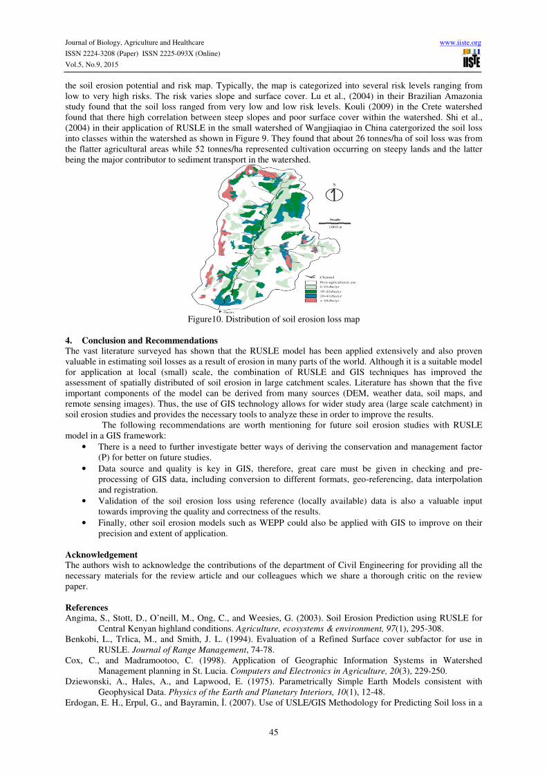
found that there high correlation between steep slopes and poor surface cover within the watershed. Shi et al.,

(2004) in their application of RUSLE in the small watershed of Wangjiaqiao in China catergorized the soil loss

into classes within the watershed as shown in Figure 9. They found that about 26 tonnes/ha of soil loss was from

the flatter agricultural areas while 52 tonnes/ha represented cultivation occurring on steepy lands and the latter

being the major contributor to sediment transport in the watershed.

Figure10. Distribution of soil erosion loss map

4. Conclusion and Recommendations

The vast literature surveyed has shown that the RUSLE model has been applied extensively and also proven

valuable in estimating soil losses as a result of erosion in many parts of the world. Although it is a suitable model

for application at local (small) scale, the combination of RUSLE and GIS techniques has improved the

assessment of spatially distributed of soil erosion in large catchment scales. Literature has shown that the five

important components of the model can be derived from many sources (DEM, weather data, soil maps, and

remote sensing images). Thus, the use of GIS technology allows for wider study area (large scale catchment) in

soil erosion studies and provides the necessary tools to analyze these in order to improve the results.

The following recommendations are worth mentioning for future soil erosion studies with RUSLE

model in a GIS framework:

• There is a need to further investigate better ways of deriving the conservation and management factor

(P) for better on future studies.

• Data source and quality is key in GIS, therefore, great care must be given in checking and pre-

processing of GIS data, including conversion to different formats, geo-referencing, data interpolation

and registration.

• Validation of the soil erosion loss using reference (locally available) data is also a valuable input

towards improving the quality and correctness of the results.

• Finally, other soil erosion models such as WEPP could also be applied with GIS to improve on their

precision and extent of application.

Acknowledgement The authors wish to acknowledge the contributions of the department of Civil Engineering for providing all the

necessary materials for the review article and our colleagues which we share a thorough critic on the review

paper.

References Angima, S., Stott, D., O’neill, M., Ong, C., and Weesies, G. (2003). Soil Erosion Prediction using RUSLE for

Central Kenyan highland conditions. Agriculture, ecosystems & environment, 97(1), 295-308.

Benkobi, L., Trlica, M., and Smith, J. L. (1994). Evaluation of a Refined Surface cover subfactor for use in

RUSLE. Journal of Range Management, 74-78.

Cox, C., and Madramootoo, C. (1998). Application of Geographic Information Systems in Watershed

Management planning in St. Lucia. Computers and Electronics in Agriculture, 20(3), 229-250.

Dziewonski, A., Hales, A., and Lapwood, E. (1975). Parametrically Simple Earth Models consistent with

Geophysical Data. Physics of the Earth and Planetary Interiors, 10(1), 12-48.

Erdogan, E. H., Erpul, G., and Bayramin, İ. (2007). Use of USLE/GIS Methodology for Predicting Soil loss in a



Vol.5, No.9, 2015

46

Semiarid Agricultural Watershed. Environmental Monitoring and Assessment, 131(1-3), 153-161.

Fu, B., Meng, Q., Qiu, Y., Zhao, W., Zhang, Q., and Davidson, D. (2004). Effects of Land use on Soil Erosion

and Nitrogen loss in the Hilly area of the Loess Plateau, China. Land Degradation and Development,

15(1), 87-96.

Fu, B., Zhao, W., Chen, L., Zhang, Q., Lü, Y., Gulinck, H., and Poesen, J. (2005). Assessment of Soil Erosion at

large Watershed Scale using RUSLE and GIS: a case study in the Loess Plateau of China. Land

Degradation and Development, 16(1), 73-85.

Fu, G., Chen, S., and McCool, D. K. (2006). Modeling the Impacts of no-till practice on Soil Erosion and

Sediment Yield with RUSLE, SEDD, and ArcView GIS. Soil and Tillage Research, 85(1), 38-49.

Gallaher, R. N., and Hawf, L. (1997). Role of Conservation Tillage in Production of a wholesome Food Supply.

PARTNERS FOR A, 23.

Gibbs, R. A., Belmont, J. W., Hardenbol, P., Willis, T. D., Yu, F., Yang, H., . . . Shen, Y. (2003). The

International HapMap project. Nature, 426(6968), 789-796.

Haan, C. T., Barfield, B. J., and Hayes, J. C. (1994). Design Hydrology and Sedimentology for Small

Catchments: Elsevier.

Ismail, J., and Ravichandran, S. (2008). RUSLE2 Model Application for Soil Erosion Assessment using Remote

Sensing and GIS. Water Resources Management, 22(1), 83-102.

Kang, S., Zhang, L., Song, X., Zhang, S., Liu, X., Liang, Y., and Zheng, S. (2001). Runoff and Sediment Loss

Responses to Rainfall and Land use in two Agricultural Catchments on the Loess Plateau of China.

Hydrological Processes, 15(6), 977-988.

Khosrokhani, M., and Pradhan, B. (2013). Spatio-temporal Assessment of Soil Erosion at Kuala Lumpur

Metropolitan City using Remote Sensing Data and GIS. Geomatics, Natural Hazards and Risk (ahead-

of-print), 1-19.

Kouli, M., Soupios, P., and Vallianatos, F. (2009). Soil Erosion Prediction using the Revised Universal Soil Loss

Equation (RUSLE) in a GIS framework, Chania, Northwestern Crete, Greece. Environmental Geology,

57(3), 483-497.

Lal, R. (1990). Soil Erosion in the Tropics: Principles and Management: McGraw Hill.

Lee, S. (2004). Soil Erosion Assessment and its Verification using the Universal Soil Loss Equation and

Geographic Information System: a case study at Boun, Korea. Environmental Geology, 45(4), 457-465.

Lewis, B. P., Burge, C. B., and Bartel, D. P. (2005). Conserved Seed Pairing, often flanked by Adenosines,

indicates that thousands of human genes are micro RNA targets. cell, 120(1), 15-20.

Lim, K. J., Sagong, M., Engel, B. A., Tang, Z., Choi, J., & Kim, K.-S. (2005). GIS-based Sediment Assessment

Tool. Catena, 64(1), 61-80.

Lu, D., Li, G., Valladares, G., and Batistella, M. (2004). Mapping Soil Erosion Risk in Rondonia, Brazilian

Amazonia: using RUSLE, Remote Sensing and GIS. Land Degradation and Development, 15(5), 499-

512.

Lufafa, A., Tenywa, M., Isabirye, M., Majaliwa, M., and Woomer, P. (2003). Prediction of Soil Srosion in a

Lake Victoria Basin Catchment using a GIS-based Universal Soil Loss Model. Agricultural Systems,

76(3), 883-894.

McCool, D., Brown, L., Foster, G., Mutchler, C., and Meyer, L. (1987). Revised Slope Steepness Factor for the

Universal Soil Loss Equation. Transactions of the ASAE-American Society of Agricultural Engineers

(USA).

Merritt, W. S., Letcher, R. A., and Jakeman, A. J. (2003). A Review of Erosion and Sediment Transport Models.

Environmental Modelling and Software, 18(8), 761-799.

Millward, A. A., and Mersey, J. E. (1999). Adapting the RUSLE to Model Soil Erosion Potential in a

Mountainous Tropical Watershed. Catena, 38(2), 109-129.

Mitasova, H., Hofierka, J., Zlocha, M., and Iverson, L. R. (1996). Modelling Topographic Potential for Erosion

and Deposition using GIS. International Journal of Geographical Information Systems, 10(5), 629-641.

Molnár, D. K., & Julien, P. Y. (1998). Estimation of upland erosion using GIS. Computers & Geosciences,

24(2), 183-192.

Moore, I. D., and Burch, G. J. (1986). Physical Basis of the Length-slope Factor in the Universal Soil Loss

Equation. Soil Science Society of America Journal, 50(5), 1294-1298.

Neshat, A., Pradhan, B., Pirasteh, S., and Shafri, H. Z. M. (2014). Estimating Groundwater Vulnerability to

Pollution using a Modified DRASTIC Model in the Kerman Agricultural Area, Iran. Environmental

Earth Sciences, 71(7), 3119-3131.

Onori, F., De Bonis, P., and Grauso, S. (2006). Soil Erosion Prediction at the Basin Scale using the Revised

Universal Soil Loss Equation (RUSLE) in a catchment of Sicily (southern Italy). Environmental

Geology, 50(8), 1129-1140.

Ozcan, A. U., Erpul, G., Basaran, M., and Erdogan, H. E. (2008). Use of USLE/GIS Technology Integrated with



Vol.5, No.9, 2015

47

Geostatistics to Assess Soil Erosion Risk in different Land uses of Indagi Mountain Pass—Cankırı,

Turkey. Environmental Geology, 53(8), 1731-1741.

Pimentel, D., Marklein, A., Toth, M. A., Karpoff, M. N., Paul, G. S., McCormack, R., . . . Krueger, T. (2009).

Food versus Biofuels: Environmental and Economic Costs. Human ecology, 37(1), 1-12.

Pradhan, B., Chaudhari, A., Adinarayana, J., and Buchroithner, M. F. (2012). Soil Erosion Assessment and its

correlation with Landslide events using Remote Sensing Data and GIS: a case study at Penang Island,

Malaysia. Environmental Monitoring and Assessment, 184(2), 715-727.

Renard, K. G., Foster, G. R., Weesies, G. A., McCool, D., and Yoder, D. (1997). Predicting Soil Erosion by

Water: A Guide to Conservation Planning with the Revised Universal Soil Loss Equation (RUSLE).

Agriculture Handbook (Washington)(703).

Renard, K. G., Foster, G. R., Weesies, G. A., and Porter, J. P. (1991). RUSLE: Revised Universal Soil Loss

Equation. Journal of Soil and Water Conservation, 46(1), 30-33.

Renard, K. G., and Freimund, J. R. (1994). Using Monthly Precipitation Data to Estimate the< i> R</i>-Factor

in the Revised USLE. Journal of Hydrology, 157(1), 287-306.

Römkens, M., Luk, S., Poesen, J., and Mermut, A. (1995). Rain Infiltration into Loess Soils from different

Geographic Regions. Catena, 25(1), 21-32.

Sauerborn, P., Klein, A., Botschek, J., and Skowronek, A. (1999). Future Rainfall Erosivity Derived from Large-

scale Climate Models—Methods and Scenarios for a Humid Region. Geoderma, 93(3), 269-276.

Shamshad, A., Leow, C., Ramlah, A., Wan Hussin, W., and Mohd Sanusi, S. (2008). Applications of

AnnAGNPS Model for Soil Loss Estimation and Nutrient Loading for Malaysian conditions.

International Journal of Applied Earth Observation and Geoinformation, 10(3), 239-252.

Smith, L. P. (1976). Agricultural Climate of England and Wales: A Real Averages, 1941-70. Technical Bulletin.

Van der Knijff, J., Jones, R., and Montanarella, L. (2000). Soil Erosion Risk Assessment in Europe: European

Soil Bureau, European Commission.

Wilson, J. P., and Lorang, M. S. (1999). Spatial Models of Soil Erosion and GIS. Spatial Models and GIS: New

Potential and New Models, 83-108.

Wischmeier, W. H., and Smith, D. D. (1978). Predicting Rainfall Erosion losses-A Guide to Conservation

Planning. Predicting Rainfall Erosion losses-A guide to Conservation Planning.

Yitayew, M., Pokrzywka, S., and Renard, K. (1999). Using GIS for Facilitating Erosion Estimation. Applied

Engineering in Agriculture, 15, 295-302.

Review of Soil Erosion Assessment using RUSLE Model and GIS

Documents

Transcript of Review of Soil Erosion Assessment using RUSLE Model and GIS