
Review of our WACC method - ipart.nsw.gov.au · Review of our WACC method IPART 1 1 Executive...
112
Review of our WACC method Final Report Research February 2018
Transcript of Review of our WACC method - ipart.nsw.gov.au · Review of our WACC method IPART 1 1 Executive...

Review of our WACC method
Final Report
Research February 2018

ii IPART Review of our WACC method
© Independent Pricing and Regulatory Tribunal of New South Wales 2017
This work is copyright. The Copyright Act 1968 permits fair dealing for study, research, news reporting, criticism and review. Selected passages, tables or diagrams may be reproduced for such purposes provided acknowledgement of the source is included.
ISBN 978-1-76049-181-9
The Tribunal members for this review are:
Dr Peter J Boxall AO, Chair
Mr Ed Willett
Ms Deborah Cope
Inquiries regarding this document should be directed to a staff member:
Mike Smart (02) 9113 7728
Melanie Mitchell (02) 9113 7743
Anthony Rush (02) 9113 7790

Review of our WACC method IPART iii
Contents
1 Executive summary 1
1.1 Key elements remain broadly the same in our 2018 method 2
1.2 Other elements will change incrementally 3
1.3 Our process for this review 8
1.4 Structure of this report 8
1.5 List of final decisions 9
2 Context and principles for this review 13
2.1 Who our final decisions affect 13
2.2 Scope of this review 13
2.3 Our principles for this review 14
3 Measuring WACC inputs 18
3.1 Overview of our final decisions on measuring WACC inputs 18
3.2 Our definition of the efficient benchmark entity 19
3.3 Synchronise sampling dates and align sampling periods 21
3.4 Continue to notify regulated businesses of sampling dates 23
4 Determining the cost of debt 24
4.1 Overview of final decisions on cost of debt 24
4.2 Maintain our midpoint method 25
4.3 Adopt a 10-year trailing average approach to calculate the historic cost of debt 26
4.4 Adopt a short-term trailing average approach to estimate the current cost of debt 29
4.5 Adopt consistent observation windows in calculating historic and current costs 36
4.6 Decide how to pass-through annual changes 38
4.7 Where we use a true-up we will discount changes by the WACC 39
4.8 Annualise bond yield data 40
4.9 Maintain a 10-year term-to-maturity 41
4.10 Continue to use 10-year coupon paying bond yields 44
4.11 Continue to use the BBB debt margin published by the RBA 45
5 Determining the cost of equity 47
5.1 Overview of final decisions on cost of equity 47
5.2 Continue to use the Sharpe-Lintner CAPM 48
5.3 Continue to determine cost of equity as midpoint between current and historic estimates 50
5.5 Modify our approach for measuring the current MRP 52
5.6 Modify our approach for selecting single value for current MRP 56
5.7 Re-estimate the equity beta at each price review 59
5.8 Use a broad selection of proxy companies to estimate the equity beta 61
5.9 Modify our approach for adjusting equity betas to mitigate estimation bias 64
6 Combining measurements to derive the WACC 66
6.1 Overview of final decisions on deriving the WACC 66
iv IPART Review of our WACC method
6.2 Maintain our 2013 method of constructing the uncertainty index 67
6.3 Maintain our current decision rule 68
6.4 Maintain our discretion to consult on out-of-range situations 68
6.5 Re-estimate the gearing ratio at each price review 73
7 Measuring inflation and gamma 75
7.1 Overview of final decisions on inflation and gamma 75
7.2 Setting a real post-tax WACC 76
7.3 Adjust for expected inflation over the regulatory period 76
7.4 Use a geometric average method to calculate expected inflation 77
Appendices 85
A Comparison of other regulators’ approaches to WACC 86
B How we will update the cost of debt measurements 92
C Our analysis on the appropriate CAPM model 95
D IPART’s uncertainty index model 99
E Our analysis on using breakeven inflation (BEI) 103

Review of our WACC method IPART 1
1 Executive summary
Since mid-2017, the Independent Pricing and Regulatory Tribunal of NSW (IPART) has been reviewing our standard method for determining the weighted average cost of capital
(WACC), with the aim of improving its accuracy and predictability.
The WACC is a key input for calculating the revenue requirements and setting prices for the businesses we regulate, and our decisions on this cost need to be as accurate as possible. If
we set the WACC too high, customers would pay too much and the regulated business
could be encouraged to over-invest. If we set it too low, the business’ financial viability could suffer, and it may under-invest. Neither outcome is in the long-term interest of
customers.
We have now completed the review and made final decisions on the method we will use in future determinations (the 2018 method).1 A small number of these decisions differ from
our draft decisions, and are generally more consistent with stakeholder views.
This report outlines our final decisions, explains how and why we made those decisions, and highlights where they differ from our draft decisions (see Box 1.1 for a summary of key
differences). Our 2018 method will apply to pricing decisions that take effect on or after
1 July 2018.2
We would like to thank all the stakeholders who participated in this review and helped to
make our final decisions an improvement on our existing WACC method. We consider that
our 2018 method can be replicated by stakeholders and will increase the accuracy and stability of the regulatory regime for the businesses we regulate.
1 We will consult on applying our 2018 method in the course of future price reviews, approaching each review
based on its unique circumstances. 2 Our 2018 method will not apply to any determination currently in effect, including our fare determinations
for private ferries and rural and regional buses, both of which apply from 1 January 2018.
2 IPART Review of our WACC method
Box 1.1 Summary of key differences between draft and final decisions
We will use a ‘trailing average’ approach to calculate both historic and current cost of debt
In response to stakeholder feedback, we made draft decisions to adjust the current cost of debt
over the regulatory period. However, stakeholders expressed concerns that this would not
sufficiently mitigate refinancing risk and maintained that the most efficient cost of debt for a
benchmark firm with long-lived assets is one based on a 10-year trailing average.a
After further consultation through a series of targeted stakeholder workshops and further analysis,
we decided we will estimate the historic cost of debt as a 10-year trailing average, and the current
cost of debt as a short-term trailing average with the length of this term matching the regulatory
period (usually 4 to 5 years).
We will update the cost of debt annually within a regulatory period and decide how annual
changes are passed through on a case-by-case basis, as part of our price review process.
Our draft decision was to cumulate annual changes in the cost of debt and pass the cumulative
change through to prices using a true-up at the beginning of the next regulatory period. Sydney
Desalination Plan (SDP) and WaterNSW submitted a strong preference for annual price
adjustments, as the delay associated with a true-up could potentially cause a firm to breach its debt
covenants.b Given the approaches should be equivalent in present value terms, we decided that
we will decide whether to apply annual price adjustments or a true-up on a case-by-case basis (as
part of the price review process). If we decide to use a true-up, we will use the WACC as the
discount rate in calculating the true-up amount.
We will provide more consultation and transparency in our equity beta and gearing
processes
Based on stakeholder feedback, we have also made some small adjustments to our processes for
re-estimating equity beta and gearing to make them more transparent, replicable and consultative.
a Sydney Water submission to IPART Draft Report, December 2017, p 3; NSW Treasury submission to IPART Draft
Report, December 2017, p 1; SDP submission to IPART Draft Report, December 2017, p 12; Hunter Water submission to
IPART Draft Report, December 2017, p 8; WaterNSW submission to IPART Draft Report, December 2017, p 4.
b SDP submission to IPART Draft Report, December 2017, p 12; WaterNSW submission to IPART Draft Report, December
2017, p 9.
1.1 Key elements remain broadly the same in our 2018 method
The feedback we received from stakeholders throughout this review confirmed our view
that, overall, the 2013 WACC method works well.3 For example, in response to our Issues
Paper, the ARTC submitted that this method has provided significant value in “stability,
logical consistency and transparency”.4
Hunter Water put the view that compared to our previous method, the 2013 method is “a far better approach to the setting of financing costs” and that it welcomed the “setting of
3 WaterNSW submission to IPART Issues Paper, August 2017, p 4; ARTC submission to IPART Issues
Paper, August 2017, p 3; Hunter Water submission to IPART Issues Paper, August 2017, p I; Sydney Water submission to IPART Issues Paper, August 2017, p 2; SDP submission to IPART Issues Paper, August 2017, p 1.
Review of our WACC method IPART 3
decision rules in the WACC formula, the use of externally available information sources for
each parameter, the inclusion of the uncertainty index and the publication of biannual
WACC updates”. It also noted that the current method “satisfies the test of replicability,
stability and transparency”.5
In response to our Draft Report, stakeholders reiterated their general satisfaction with the
2013 method. For instance, Sydney Water commented:
IPART’s existing WACC methodology works well, incentivising improved financial efficiency and
stability. These sentiments have been echoed by our external rating agency, which have
maintained our generally stable credit rating.6
PIAC considered that:
…the stability and consistency of the WACC are generally positive outcomes for consumers, [and
stressed] the importance of keeping the WACC no higher than necessary, particularly to support
affordability and allow households to effectively budget for the essential service of water.7
Therefore, in line with our draft decisions, we will maintain key elements of the 2013
method, including the existing approaches for:
defining our benchmark firm
constructing our uncertainty index and applying our WACC decision rule
determining industry-specific parameters of gearing and equity beta, and
using a real post-tax framework and accounting for imputation credits.
We consider maintaining the stability, certainty, replicability and predictability of our
WACC method is important, as well as ensuring it produces reasonably accurate estimates.
The stability and transparency of having a standard WACC method has been an important factor in supporting a strong credit rating for some of our regulated water businesses.
1.2 Other elements will change incrementally
We have identified, analysed and consulted on opportunities to make incremental changes to some elements of our WACC method to improve its overall accuracy, transparency or
predictability. In line with our review objectives, we aimed to limit these changes to areas
where there were convincing reasons for change to increase accuracy, or enhance stability and certainty. However, where we were satisfied a change would, on balance, result in a
more accurate WACC without causing a significant adjustment for stakeholders (that is, no
windfall gains or losses, and the change could be implemented simply), we decided to
change our method.
Where we found the case for change was not strong – that is, where it was not clear that a
potential change would produce a more accurate WACC estimate with only minor adjustment impacts – we opted to maintain our 2013 method.
5 Hunter Water submission to IPART Issues Paper, August 2017, p i. 6 Sydney Water submission to IPART Draft Report, December 2017, p 1. 7 PIAC submission to IPART Draft Report, December 2017, p 1.

4 IPART Review of our WACC method
As already noted, some of our final decisions differ from our draft decisions (see Box 1.1).
Specifically, we decided:
In measuring WACC inputs, to synchronise sampling dates and periods for measuring
selected current parameters.
In determining the cost of debt, to estimate both the historic and current cost using a
trailing average approach; decide how annual changes in this cost during the
regulatory period will be passed through to prices on a case-by-case basis as part of our review process; and annualise bond yield data derived from semi-annual rates of
return.
In determining the cost of equity, to adjust our method for measuring the current market risk premium (MRP) to reduce bias; to modify our process and method for re-
estimating equity beta at each price review to improve its transparency, reliability and
accuracy.
In measuring inflation, to use the expected rate of inflation over the regulatory period;
and to calculate this rate using an approach consistent with the AER’s approach.
1.2.1 Synchronise sampling dates and periods for selected current parameters
Because market observations tend to be volatile, the timing of the observations we use to
measure the market-based parameters is important, particularly for current parameters. Under our 2013 method, we used the most recent available data for each parameter, which
means the sampling dates differed across parameters.
We made draft decisions to synchronise the sampling dates for five parameters – the risk-
free rate, debt margin, current MRP, inflation and uncertainty index – and to adopt aligned
sampling periods of 40 working days each calendar year for the risk-free rate, and two
months for the debt margin. Given stakeholder support8, we have decided to make these changes. In our view, they will improve the accuracy in our resulting WACC calculations
by recognising the interrelationships between parameters.
1.2.2 Estimate both the historic and current cost of debt using a trailing average
approach
Our 2013 method set a cost of debt as the midpoint between our estimates of the historic and
current cost unless there is significant economic uncertainty, and did not update this cost
during the regulatory period. In response to stakeholder feedback that this approach creates a refinancing risk for regulated businesses,9 we have made final decisions to estimate both
the historic and current cost of debt using a trailing average approach, which will update the
cost of debt annually over the regulatory period.
We will estimate the historic cost of debt as a 10-year trailing average by splitting the
historic cost of debt into 10 equal tranches, with the commencement and maturity dates for
8 SDP submission to IPART Draft Report, December 2017, p 12; Hunter Water submission to IPART Draft
Report, December 2017, p 8; WaterNSW submission to IPART Draft Report, December 2017, p 5. 9 NSW Treasury submission to IPART Issues Paper, August 2017, p 1; WaterNSW submission to IPART
Issues Paper, August 2017, p 9; Sydney Water submission to IPART Issues Paper, August 2017, pp 11-12; Hunter Water submission to IPART Issues Paper, August 2017, p 5.
Review of our WACC method IPART 5
each tranche staggered by one year. At the beginning of each year of the regulatory period,
the oldest tranche of debt will mature, and a new tranche will replace it.
We will estimate the current cost of debt as a short-term trailing average in a similar way.
We will split the current cost of debt into a number of equal tranches equal to the number of years in the regulatory period, with the commencement and maturity dates staggered by
one year. At the beginning of each year, the oldest tranche of debt will mature, and a new
tranche will replace it.
For both estimates, we will estimate the interest rate for each annual tranche of debt using a
40 working day observation window that we choose. We will give firms confidential,
advance notice of this window.
As the change to our approach for estimating the historic cost of debt is not likely to have a
major impact on firms or customers, we will implement it without a transition period.
However, we will transition to a short-term trailing average for the current cost of debt over one regulatory period.
We consider that these changes:
will increase the accuracy of our cost of debt estimates as an incremental improvement to our 2013 method
will increase replicability of our estimates by reducing refinancing risk for firms
will not create any windfall gains or losses to firms or customers, and
can be implemented simply.
1.2.3 Decide how to pass annual changes in the cost of debt through to prices on a
case-by-case basis, as part of our review process
As noted above, adopting a trailing average approach will update the cost of debt annually over the regulatory period. We considered whether we should update prices to reflect the
updated cost of debt annually, or use a regulatory true-up in the notional revenue
requirement for the next period, which we would pass through to prices at the beginning of the next period. We have decided to determine the most appropriate option on a case-by-
case basis, as part of our price review process. Where we decide to use a true-up, we will
use the WACC as the discount rate for calculating the true-up.
As noted above, our 2018 method will apply only to determinations made on or after
1 July 2018. Determinations already in effect will be subject to our 2013 method. This means
at the next regulatory review, there will be no true-up of the cost of debt in current determinations. Rather, the true-up will be calculated throughout the next regulatory
period and prices adjusted at the subsequent period.
1.2.4 Annualise bond yield data
We have decided to modify our approach for estimating the cost of debt by converting
published bond yield data into annualised yields. We will continue to use RBA-published
6 IPART Review of our WACC method
data on the spread between the yield of BBB rated bonds issued by Australian non-financial
corporations to the 10-year Australian Government Bond yield.
1.2.5 Adjust our method for measuring the current MRP
Under our 2013 method, we estimated the current MRP using six different methods, five of
which are variations of a dividend discount model (DDM) method, and one of which is a
market indicators method. We determined a point estimate by selecting the midpoint of the highest and lowest of these estimates in each month.
We considered several alternative methods, including selecting the median of all six
estimates, and using a weighted average of the market indicators MRP estimate and the median of the DDM MRP estimates. We decided to:
combine the DDM MRP estimates into one estimate using a median approach that
does not exclude outliers, and
set the point estimate as the weighted average of the market indicators MRP and the
median DDM MRP, with a one-third weight to the former and two-thirds weight to
the latter.
These changes are in line with our draft decisions. Most stakeholders supported these draft
decisions,10 but SDP argued we should maintain our existing approach of using the
midpoint, and weighting all estimates equally.11 After considering SDP’s submission, we maintain our view that giving all six estimates equal weight could place too much emphasis
on the DDM results. We considered SDP’s reasoning that the median is not appropriate, if
there are no consistent outliers.12 However, we consider that during and after the GFC, the
Bloomberg MRP estimate was consistently the high estimate, sitting significantly higher
than the others in the group. As such, we consider that it was a genuine outlier at that time
and the mean approach would have given it too much weight.
We have also decided to replace two of the indicators in our market indicator method (the
dividend yield and the risk-free rate) with a single new indicator (earnings yield less the
risk-free rate).
1.2.6 Modify our process and method for re-estimating the equity beta at each price
review
In our 2013 method, we assessed the equity beta each time we determined the WACC for a
regulated business to check that it remained appropriate, in light of updated market data,
and having regard to other regulators’ recent WACC decisions. We only changed the value
we used in our WACC calculations where we considered there was sufficient evidence to
support this.
10 WaterNSW submission to IPART Draft Report, December 2017, p 15; Hunter Water submission to IPART
Draft Report, December 2017, p 11; Sydney Water submission to IPART Draft Report, December 2017, p 5. 11 SDP submission to IPART Draft Report, December 2017, p 13. 12 Frontier Economics, IPART review of the WACC method – Response to Draft Report: Report prepared for
Sydney Desalination Plant, December 2017.
Review of our WACC method IPART 7
While we decided to maintain this approach, we have made some changes to the timing and
transparency of our consultation process on the equity beta. We also decided to broaden the
sample of proxy firms we use in estimating the equity beta, and discontinue considering the
Blume-adjusted equity beta.
Broaden the sample of proxy firms
One of the main weaknesses of our current approach for estimating the equity beta is that the selected proxy companies may not represent a benchmark firm well, leading to an
inaccurate estimate. To address this weakness, we have decided to use the broadest possible
selection, but exclude thinly traded stocks in line with feedback from Frontier Economics (on behalf of SDP).13 We agree that a broad sample method is more objective, more likely to
yield statistically reliable estimates, and more resistant to problems caused by companies
dropping out of the sample over time (for example, because they become de-listed).
Discontinue consideration of the Blume-adjusted equity beta
Several studies have found equity betas obtained from ordinary least squares (OLS) regression analysis are likely to be subject to a high degree of estimation bias due to
sampling error. Regulators commonly adjust for this bias using the Vasicek and/or Blume
methods.
Our 2013 method was to make a judgement on the appropriate equity beta by considering
each of the OLS equity betas with no adjustments, the Blume-adjusted equity beta and
Vasicek-adjusted equity beta. We have decided to discontinue considering the Blume-adjusted equity beta because it is an automatic, formulaic and arbitrary adjustment. We
consider that the Vasicek adjustment is preferable because it relies on firm-specific
information to adjust the empirical results.
1.2.7 Use the expected rate of inflation over the regulatory period
Under our 2013 method we deflated our nominal WACC inputs by applying a single, forward-looking rate that is the expected rate of inflation over the next 10 years, regardless
of the length of the regulatory period. We calculated expected inflation as the geometric
average of the inflation rate.
In response to our Issues Paper, Sydney Water submitted that we should use a best estimate
of expected inflation over the regulatory period rather than 10 years. It also noted our
existing method might be problematic when long-term inflation expectations differ substantially from forecast inflation over the regulatory period.14 We agree with Sydney
Water’s view, and have decided to use the expected rate of inflation over the regulatory
period. We note that this could mean we use a slightly different inflation rate in two concurrent reviews, if we decide to set different regulatory periods for the businesses
concerned.
13 Frontier Economics, Review of WACC method: response to IPART Issues Paper: A Report Prepared for
Sydney Desalination Plant, August 2017, p 39. 14 Sydney Water submission to IPART Issues Paper, August 2017, p 18.
8 IPART Review of our WACC method
1.2.8 Calculate the rate of inflation using an approach consistent with the AER’s
We have decided to calculate the expected rate of inflation by first calculating the geometric
average of the forecast change in the level of prices over the regulatory period, and then converting this average into an annual inflation rate separately. Most stakeholders
supported this approach, which is consistent with the AER’s approach.
To improve clarity, we have also decided to define the forecast we use in estimating inflation, as the inflation forecast in the RBA’s most recently issued Statement of Monetary
Policy (SMP) that is closest to 12 months from the start the regulatory period.
In response to our Issues Paper, some stakeholders suggested that we should use a ‘breakeven inflation’ (BEI) method, which is estimated by comparing yields on nominal
bonds to those on inflation-linked bonds.15 On balance, we consider that while the BEI
method has merit in theory, there may be some problems with implementing it currently, and our 2013 method promotes greater stability and predictability for stakeholders.
However, we will consider whether we should move to a break-even inflation method at our
next WACC review. Most stakeholders supported this approach.16
1.3 Our process for this review
In conducting this review, we undertook public consultation and extensive analysis. The
key steps in our process were:
Releasing an Issues Paper in July 2017, which set out our approach, proposed
principles for the review and key issues on which we sought feedback. We received
seven submissions.
Holding a public hearing in August 2017 to provide stakeholders with an opportunity
to discuss our Issues Paper, propose changes and raise further issues.
Considering all submissions to the Issues Paper, feedback from the public hearing and conducting our own analysis and research to inform our draft decisions.
Releasing a Draft Report in October 2017, which set out the analysis and reasoning for
our draft decisions, on which we sought feedback. We received six submissions.
Holding two informal workshops with stakeholders to discuss our draft decisions,
particularly on the cost of debt, and work through implementation issues.
Considering all submissions to the Draft Report and feedback from workshops, and conducting further analysis to form our final decisions.
1.4 Structure of this report
The rest of this report discusses the review in more detail and sets out our analysis and final decisions:
15 WaterNSW submission to IPART Issues Paper, August 2017, p 13; Hunter Water submission to IPART
Issues Paper, August 2017, p 10; NSW submission to IPART Issues Paper, August 2017, p 6. 16 Sydney Water submission to IPART Draft Report, December 2017, p 6; WaterNSW submission to IPART
Draft Report, December 2017, p 15; Hunter Water submission to IPART Draft Report, December 2017, p 12, SDP submission to IPART Draft Report, December 2017, p 14; PIAC submission to IPART Draft Report, December 2017, p 3

Review of our WACC method IPART 9
Chapter 2 provides contextual information about our WACC method and our
principles for this review.
Chapter 3 focuses on our approaches for measuring WACC inputs, including our
definition of the benchmark firm and the timing of market observations.
Chapters 4 and 5 discuss our approaches for determining the costs of debt and equity
respectively.
Chapter 6 discusses how we combine debt and equity measurements to derive a point estimate of the WACC, including how we implement the WACC decision rule.
Chapter 7 focuses on our approaches for measuring inflation and gamma.
1.5 List of final decisions
For convenience, a complete list of our final decisions is provided below.
Measuring WACC inputs
1 Maintain our definition of the efficient benchmark firm as ‘a firm operating in a
competitive market and facing similar risks to the regulated business. 21
2 Synchronise the sampling dates for the risk-free rate, debt margin, current MRP,
inflation and the uncertainty index. 23
3 Adopt a sampling period of 40 working days from the sampling date for the risk-free rate
and 2 months for the debt margin, aligning the start and end of the sampling periods as
closely as possible. 23
4 Continue to provide regulated businesses with confidential, advance notice of the
sampling dates. 23
Determining the cost of debt
5 Continue to estimate the cost of debt as the midpoint of our estimates of the current and
historic cost of debt when our uncertainty index is at, or within one, standard deviation
of its long-term average. 26
6 Estimate the historic cost of debt using a trailing average approach that involves: 29
– splitting the historic debt into 10 equal tranches, each with a 10-year term to maturity 29
– staggering the commencement and maturity dates for each tranche by one year, and 29
– refinancing one tranche at the beginning of each year. 29
7 Estimate the current cost of debt using a short-term trailing average approach that
involves: 36
– splitting the current debt into tranches equalling the number of years in the regulatory
period, each with a 10-year term to maturity, and 36
– staggering the commencement and maturity dates for each tranche so that at the
beginning of each year of the regulatory period, the interest rate on the oldest

10 IPART Review of our WACC method
tranche of debt will reprice at the prevailing interest rate on the new tranche of
debt. 36
8 For the current cost of debt, maintain a 40-working day observation window for the risk-
free rate and an equivalent two-month observation window for the debt risk premium
and: 37
– choose the exact timing of the observation window 37
– inform the regulated firm in advance on a confidential basis. 37
9 For the historic cost of debt, adopt a 40-working day observation window for the risk-
free rate and an equivalent two-month observation window for the debt risk premium for
each new point in the trailing average calculation and: 38
– choose the exact timing of the observation window 38
– inform the regulated firm in advance on a confidential basis. 38
10 Update the regulatory cost of debt annually, and decide whether to pass through
changes via annual price adjustments or a true-up in the subsequent period: 39
– as part of the price determination, and 39
– on a firm-by-firm basis. 39
11 Where a true-up is used to pass through changes in the cost of debt, the discount rate
used to calculate the true-up amount will be the firm’s regulatory WACC. 40
12 Convert published bond yield data into annualised yields. 41
13 Continue to use a 10-year term to maturity to estimate the cost of debt. 44
14 Continue to use the 10-year coupon-paying bond yield data to estimate the cost of debt. 45
15 Continue to use the 10-year BBB corporate bond spreads published by the RBA to
measure the debt margin across all industries. 46
Determining the cost of equity
16 Continue to use the Sharpe-Lintner CAPM to estimate the cost of equity, and monitor
the impact that the Fama-French model would have if we adopted it at a future review. 50
17 Continue to estimate the cost of equity as the midpoint between our estimates of the
current and historic cost of equity when the uncertainty index is at, or within one
standard deviation of its long-term average. 51
18 Maintain our 2013 method of keeping the cost of equity fixed during the regulatory
period. 51
19 Continue to use a range with a midpoint of 6% as the estimate of historic MRP. 52
20 Continue to use our existing six methods to measure the current MRP. 55

Review of our WACC method IPART 11
21 Continue to use the ASX 200 share price index and consensus earnings per share
forecasts to measure the current MRP using the Damodaran and Bloomberg methods
and the two Bank of England methods. 55
22 Modify the indicators we use to measure the current MRP using the market indicator
method by replacing two of our existing indicators – the dividend yield and the risk-free
rate – with one new indicator – the earnings yield less the risk-free rate. 56
23 In combining different DDM MRP estimates, move from the midpoint to a median
approach, but do not exclude outliers. 59
24 Determine the point estimate of current MRP as the weighted average of the market
indicators MRP and the median DDM MRP, with a one-third weight to the market
indicators MRP and two-thirds weight to the median DDM MRP. 59
25 Continue to re-estimate equity betas at each price review to inform our assessment of
whether the existing estimates remain appropriate. 61
26 Use the broadest possible selection of proxy companies to estimate equity beta, but
exclude thinly traded stocks. 64
27 Adopt a proxy selection process that includes: 64
– publishing our criteria for proxy selection, and our list of comparator companies that
meet our criteria at the start of the relevant review, and 64
– giving stakeholders the opportunity to propose additional comparable industries that
meet our criteria. 64
28 Determine the appropriate equity beta having regard to equity betas calculated using
the OLS method with the Vasicek adjustment. 65
Combining measurements to derive the WACC
29 Maintain our 2013 method of constructing the uncertainty index. 67
30 Maintain our 2013 method decision rule. 68
31 Continue to use our discretion to determine the appropriate weighting of current and
historic average market data when the market is in an abnormal state, and to consult
with stakeholders before we make our decisions. 70
32 Continue to re-estimate the gearing of the benchmark entity at each price review to
inform our assessment of whether the existing estimates remain appropriate. 74
Measuring inflation and gamma
33 In converting our nominal WACC inputs into real terms, adjust them by the expected
rate of inflation over the regulatory period. 77
34 Calculate the average expected inflation rate as the geometric average of: 80

12 IPART Review of our WACC method
– the RBA’s 1-year ahead inflation forecast in its most recently issued Statement of
Monetary Policy for the first year of the regulatory period, and 80
– the midpoint of the RBA’s target inflation band (2.5%), for the remaining years in the
regulatory period. 80
35 Reconsider whether we should move to a break-even inflation method to calculate the
average expected inflation rate at the next review of our WACC method. 80
36 Calculate expected inflation as the geometric average of the change in the level of
prices. 81
37 Define the 1-year ahead RBA forecast we use to estimate inflation, as the inflation
forecast: 81
– in the RBA’s most recently issued Statement of Monetary Policy, and 81
– that is closest to 12 months ahead of the start of the regulatory period. 81
38 Continue to use 0.25 as the value for gamma. 83

Review of our WACC method IPART 13
2 Context and principles for this review
Our consultations during this review confirmed that our existing 2013 method is generally working well and has resulted in reasonably accurate decisions in the past. Stakeholders
can replicate our calculations, and the method has increased the stability of the regulatory
regime for our regulated businesses.
Our objective for this review was to identify whether there are opportunities to make
incremental improvements to the method so our WACC decisions better reflect efficient
financing costs. We developed an approach for meeting this objective, including a set of principles to guide our decision making.
2.1 Who our final decisions affect
Our WACC decisions have a major impact on the returns on assets for our regulated businesses and others affected by our building block calculations. These regulated
businesses include:
water utilities such as Sydney Water Corporation, WaterNSW, Hunter Water Corporation and the Sydney Desalination Plant (SDP), and
public transport businesses such as Transport for NSW and private ferries.
Other affected businesses include those we review under section 9 of the Independent Pricing
and Regulatory Tribunal Act 1992 (IPART Act), such as the Port Authority of NSW, for which
we recently recommended maximum fees and charges for cruise ships.
Our WACC decisions also have a major impact on the customers of our regulated businesses. The allowance for a return on assets within the revenue requirement
significantly affects the prices these businesses can charge.
2.2 Scope of this review
The review focussed on how we measure and estimate the parameters we use to calculate
the WACC. Its scope included:
our basis for measurement, including our definition of the benchmark firm and approach to sampling
how we estimate the parameters for the cost of debt and the cost of equity
how we bring these parameters together to select a single point estimate of the WACC, and
how we measure inflation and gamma.
We did not consider broader policy issues related to how we apply the WACC. For example, the type of WACC we apply (ie, whether it is pre- or post-tax, real or nominal) and

14 IPART Review of our WACC method
matters associated with our building block method (such as financeability) were outside the
scope.
We are satisfied that applying a post-tax WACC more closely estimates tax paid by a
benchmark firm than applying a pre-tax WACC using the statutory tax rate. We also consider that it is appropriate to maintain our approach of setting a real WACC and
indexing the asset base for inflation. Moreover, moving away from a real post-tax WACC
would add considerably to uncertainty and have the potential for large price changes.
2.3 Our principles for this review
In making our decisions for this review, we aimed to balance the following four principles:
1. Our WACC method should produce estimates of the cost of capital that are as
reasonably accurate as possible. This will ensure that customers do not pay more than
necessary and that the regulated firms will be financially viable and have the incentive
to invest in the efficient level of productive assets.
2. Our WACC method should be relatively stable over time to give stakeholders
certainty.
3. Our WACC method should be predictable and replicable by stakeholders to provide transparency and reduce resources required in each review.
4. We should make incremental improvements where there is sufficient evidence that
they increase the accuracy of the cost of capital faced by a benchmark firm.
We consider these principles take account of the impact of our WACC method on regulated
business and their customers, and take account of the matters we are required to consider in
making our determinations and recommendations under section 15 of the IPART Act (see Box 2.1).
We added the first principle listed above following PIAC’s submission to our Issues Paper,
which suggested that we should:
…emphasise the impact on consumers from any changes to the WACC method in this review.
This should help to frame the debate to ensure that the WACC methodology is, indeed, working in
the best interest of consumers.17
PIAC welcomed the inclusion, stating:
Keeping this principle central to the review should help minimise risk that stakeholders lose sight of
the overarching role of the WACC in regulatory price and revenue determinations and instead
become caught up in an academic or technical debate over which method or model is inherently
‘better’ .18
Each principle, and our rationale for including it, is discussed in more detail below.
17 PIAC submission to IPART Issues Paper, August 2017, pp 1-2. 18 PIAC submission to IPART Draft Report, December 2017, p 1.

Review of our WACC method IPART 15
Box 2.1 Matters we are required to consider under section 15 of the IPART Act
There are several matters we are required to consider in making our determinations and
recommendations. Under section 15 of the Independent Pricing and Regulatory Tribunal Act 1992
(IPART Act) we must have regard to a range of factors, including, but not limited to:
1. cost of providing the services concerned
2. protection of consumers from abuses of monopoly power
3. appropriate return on public sector assets and associated dividends to the Government for
the benefit of the people of New South Wales
4. need for greater efficiency in the supply of services so as to reduce the costs for the benefit
of consumers and taxpayers, and
5. impact on borrowing, capital and dividend requirements of the government agency
concerned and, in particular, the impact of any need to renew, or increase relevant assets.
The cost of capital is a component of the costs of providing the services. Setting the WACC too
high is arguably inconsistent with (2) and (4), while setting it too low may conflict with (3) and (5).
The requirement to consider efficiency influences our definition of the benchmark entity and how
we measure the WACC parameters.
Source: Independent Pricing and Regulatory Tribunal Act 1992, section 15.
2.3.1 Our WACC method should produce as reasonably accurate as possible
estimates
Our overarching objective in setting the WACC is to produce a reasonably accurate estimate.
This is important because, if we set a WACC that is too high, then customers would pay too
much for the services and we risk encouraging too much investment in that business. If we
set the WACC too low, then we risk the financial viability of the firm and encouraging too
little investment. Neither of these outcomes is in the long term interest of consumers.
2.3.2 Our WACC method should be stable over time to provide stakeholder
certainty
Having a stable WACC method within and between regulatory periods provides certainty to
regulated businesses and their customers. Increased certainty translates to reduced risk, stable revenues for businesses and stable prices for customers.
For example, regulatory stability is an important influence on the credit ratings of Australian
water utilities. Moody’s rating agency’s ‘Regulated Water Utilities’ methodology assigns a
15% weight to ‘stability and predictability of regulatory environment’.19
Following the implementation of our 2013 WACC method, in March 2015, Moody’s
upgraded Sydney Water Corporation’s (Sydney Water) issuer rating from A1 to Aa3. It attributed this upgrade to Sydney Water’s “expectation of improved transparency in the
regulatory framework”. Moody’s commented that:
IPART has been demonstrating increased predictability and transparency in its regulatory
decisions. Although it does not have the track record of the Australian Energy Regulator which
19 Moody’s Investor Service, Rating Methodology – Regulated Water Utilities, December 2015, p 6.

16 IPART Review of our WACC method
regulates transmission and distribution electricity and gas networks in the eastern and southern
states, it has shown a philosophy that has become increasingly transparent, and supportive of the
credit profiles of regulated entities, including Sydney Water.20
Similarly, Moody’s March 2015 rating report for Hunter Water Corporation (Hunter Water) stated that IPART has “a stable and mature regulatory framework…”21 and “we believe that
IPART will continue to exhibit consistency in its decision translating into increased stability
in revenue outcomes for Hunter Water.”22
In October 2016, Moody’s changed its outlook for Sydney Water to stable, stating:
The change in outlook to stable reflects Moody's belief that Sydney Water's shareholder, the New
South Wales state government (New South Wales Treasury Corporation (TCorp), Aaa stable), will
implement countermeasures to maintain the company's metrics within its rating tolerance level.
…the rating recognizes that the transparent regulatory framework which governs Sydney Water's
regulated tariffs provides visibility into likely future revenue reductions and space to implement the
required countermeasures to protect its credit profile.23
Sydney Water agreed, stating that “IPART’s existing WACC methodology works well,
incentivising improved financial efficiency and stability. These sentiments have been echoed by our external rating agency, which have maintained our generally stable credit
rating”.24
We have not made broad changes to our WACC method to ensure its ongoing stability.
2.3.3 The WACC should be predictable and replicable by stakeholders for
increased transparency
In our 2013 WACC review, we decided to publish financial market updates biannually in
February and August.25 We publish these updates to allow our stakeholders to better replicate and anticipate our WACC decisions. In conjunction with the updates, we also
release a WACC spreadsheet with a working copy of our WACC model.
This enables stakeholders to understand how our WACC decisions are made. It reduces the resources and effort required by stakeholders in each regulatory review. This has been
beneficial for both IPART and the regulated businesses. As discussed above, it has also had
a positive impact on the ratings outlook for water utilities, with Moody’s specifically referencing IPART’s improvement of “the transparency and predictability of its revenue
decisions” in its reasoning for changing the Sydney Water rating outlook from stable to
positive.26 It stated that:
20 Moody’s Investor Service, Rating Action: Moody’s upgrades Sydney Water’s rating to Aa3; outlook stable,
March 2015, p 1. 21 Moody’s Investor Service, Rating Action: Moody's assigns first-time A1 issuer rating to Hunter Water
Corporation; Outlook Stable, March 2015, p 1. 22 Ibid. 23 Moody’s Investor Service, Rating Action: Moody's changes outlook for Sydney Water Corp's Aa3 rating to
Stable, October 2016, p 1. 24 Sydney Water submission to Draft Report, December 2017, p 1. 25 IPART, Review of WACC Methodology – Final Report, December 2013, p 29. 26 Moody’s Investor Service, Moody's revises Sydney Water's rating outlook to positive from stable,
December 2014, p 1.
Review of our WACC method IPART 17
The improvement in IPART's transparency is reflected in a number of measures that the regulator
has taken in the last 1-2 years, including the bi-annual publication of its financial market updates,
following a review of its weighted average cost of capital ("WACC") methodology. As a result, the
improvement in the transparency of the regulatory framework is enhancing Sydney Water's credit
profile, which also factors in our expectation for continued stability in its financial metrics.27
In making our decisions for this review, we sought to maintain or improve our current
transparency, predictability and replicability.
2.3.4 We should make incremental improvements where there are convincing
reasons
While our WACC method has generally performed well over time, we noted in our Issues
Paper and Draft Report that there was scope to improve it incrementally. We have made
improvements only where we have found that there are convincing reasons for change to increase accuracy, or enhance stability and certainty.
There are many differences between the approaches individual regulators take to calculating
the WACC. This makes it difficult to be consistent with other regulators when making our WACC decisions. However, as part of this review we considered recent changes that other
Australian and New Zealand regulators have made to their WACC approach, and the
evidence and reasons for these changes (See Appendix A).
While stakeholders considered that a consistent approach across regulators would be
beneficial, we consider that we should pursue it only where it leads to an improvement. In
response to our Issues Paper, Sydney Water stated its view that:
…generally harmonising positions across regulators is beneficial, in so far as harmonisation brings
about improvements to IPART’s WACC method. That is, change towards regulatory best
practice.28
Hunter Water stated:
Regulators should continually review and benchmark their methodologies against peers to
encourage robust outcomes in their respective jurisdictions. A common position across regulators
when it occurs should indicate a best practice position, however should not be promoted for the
sake of consistency.29
Water NSW stated:
We think that there should be a race to best-in-class, and that it is better to have a regulatory
environment that is ‘better-and-different’, than the ‘same-and-worse’.30
We agree with these views and have proposed changes only where they would improve the accuracy of our WACC estimate.
27 Ibid.
28 Sydney Water submission to IPART Issues Paper, August 2017, p 8 29 Hunter Water submission to IPART Issues Paper, August 2017, p A.2 30 WaterNSW submission to IPART Issues Paper, August 2017, p 5
18 IPART Review of our WACC method
3 Measuring WACC inputs
We use two types of inputs for our WACC calculation: industry-specific parameters, and market-based parameters. The industry-specific parameters include the gearing ratio and
the equity beta. We measure these parameters by studying a benchmark entity, rather than
the actual regulated firm. The market-based parameters include the risk-free rate, debt margin, market risk premium (MRP) and inflation forecast. We base these parameters on a
sample of market observations or forecasts.
As part of this review, we have considered:
our definition of the benchmark entity, particularly whether we should assume that it
operates in a competitive or regulated market, and
our approach to sampling the market observations, including whether the sampling dates for all parameters should be synchronised, and whether these dates should be
disclosed to regulated businesses in advance.
The sections below provide an overview of decisions on these issues, and then discuss them in detail.
3.1 Overview of our final decisions on measuring WACC inputs
We have decided to maintain our definition of the benchmark entity. We consider this definition is consistent with our price setting objective, and stakeholders expressed strong
support for maintaining it.
However, we have also decided to make two changes to our approach to sampling market observations. These are to:
synchronise the sampling dates for the risk-free rate, debt margin, current MRP,
inflation and the uncertainty index, and
adopt a consistent sampling period of 40 working days and 2 months from the
sampling date for the risk-free rate and debt margin, respectively, so that the sampling
periods closely align.31
We consider these modifications would improve the accuracy of our WACC decisions by
recognising the co-relationships between parameters.
In addition, we will continue to provide regulated businesses with advance notice of the sampling dates we will use, but not make this information public until we release our
determinations. We consider this would allow businesses to manage their debt portfolios
without exposing them to undue financing risk.
31 We measure some parameters daily and others monthly, depending on the data source.

Review of our WACC method IPART 19
These final decisions are a slight modification from our draft decisions, taking into account
our final decisions on how we calculate our cost of debt.
3.2 Our definition of the efficient benchmark entity
Our 2013 method estimates the WACC with reference to an efficient benchmark entity, which we define as ‘a firm operating in a competitive market and facing similar risks to the
regulated business’. The cost of capital for this firm may be different to the regulated
business’ actual cost. This is consistent with our price setting objective, which is to attempt to replicate the disciplines of a competitive market. A competitive market would limit
prices to the level of efficient and prudent costs. This could differ from the costs incurred by
the actual business.
Because the benchmark entity is a hypothetical firm, its cost of capital cannot be observed
directly. Therefore, we rely on information on a sample of proxy firms to determine the
industry-specific WACC parameters. How we define the benchmark efficient entity is important, as it guides our selection of these proxy firms.
3.2.1 Other regulators use a different definition
Our definition of the benchmark firm differs from those used in some other Australian
jurisdictions. For example, the AER adopts ‘a conceptual definition of the benchmark
efficient entity that is a pure play, regulated energy network business operating within Australia’.32
The AER’s reasoning is that demand risk is mitigated by the regulatory regime through
revenue or price setting mechanisms under a revenue cap. Energy network businesses can use higher fixed charges to offset demand volatility under a price cap and have the ability to
propose the form of control they employ (eg, revenue cap or price cap). By virtue of being
regulated, these businesses effectively face a very limited increase in risk due to competition.33
The Queensland Competition Authority (QCA) uses similar guidance in choosing proxy
firms for benchmarking, being ‘pure play’, ‘regulated’ and ‘standalone’ firms.34
The Essential Services Commission of South Australia (ESCOSA) applies a set of operational
principles for setting a rate of return, which include that ‘The rate of return should reflect
the prudent and efficient financing strategy of an incumbent large water utility which minimises expected costs in the long-term, on a risk-adjusted basis’.35 Further, ESCOSA’s
operational principles state that ‘The assumed prudent financing strategy should not
depend on the ownership of the regulated business (ie, the approach is indifferent to whether the entity is in Government or private ownership).’36
32 AER, Better Regulation, Explanatory Statement - Rate of Return Guideline, December 2013, p 32. 33 Ibid, p 33. 34 Queensland Competition Authority, Final decision, Trailing average cost of debt, April 2015, p 6. 35 Essential Services Commission of South Australia, SA Water Regulatory Rate of Return 2016 – 2020, Final
Report to the Treasurer, March 2015, p 21. 36 Ibid, p 22.

20 IPART Review of our WACC method
3.2.2 Stakeholders supported our existing definition
Stakeholders generally supported our current definition.37 For example, Sydney Water
stated:
We believe, complying with IPART’s definition will promote efficient financing practices for Sydney
Water and deliver long term benefits to our customers. Further we agree with IPART’s rationale
that it is not necessary to be fully consistent with other regulators.38
Hunter Water stated:
Hunter Water’s submission to IPART’s issues paper also noted the importance of ensuring that the
benchmark entity takes into consideration the risks of investing in and operating infrastructure
assets. This will recognise the risks of substantial up-front costs and capital investment, long lives
of assets and long and detailed planning process which drives investment decision making in a
regulated business such as Hunter Water.39
PIAC considered that our preliminary view was ‘not inappropriate’.40
3.2.3 Our final decision is to maintain our existing definition
We maintain our view that our current definition is appropriate. The underlying rationale for this definition is that, if the regulated utility was subject to competition instead of
regulation, then it would be able to pass only efficient capital costs through to customers.
We note that IPART operates under different legislation to that of the AER, QCA and ESCOSA in regulating energy utilities and we regulate a broader cross-section of businesses.
In setting prices, we can aim to replicate the outcomes of a competitive market and choose
proxy companies that reflect similar risks to those established under our regulatory framework.
We prefer our definition for two reasons:
1. It is consistent with our price setting objective, which is to replicate the outcomes of a competitive market. Our definition aims to ensure that a regulated firm faces similar
investment incentives to a competitive firm facing similar risks. This approach
replicates the outcomes of a competitive market and avoids creating possible distortions between the regulated and competitive sectors of the economy. This
encourages an efficient allocation of capital across the economy.
2. There are more listed businesses in the competitive sector than in the regulated sector. This means that analysis of firms in the competitive sector benefits from a larger set of
observations of the cost of capital and financing strategies.
We consider that it is appropriate to include non-regulated firms (those operating in a competitive market) and relevant regulated firms in the set of proxy firms. This is because:
37 WaterNSW submission to IPART Issues Paper, August 2017, p 7; SDP submission to IPART Issues Paper,
August 2017, p 13; PIAC submission to IPART Issues Paper. August 2017, p 2; Sydney Water, submission to IPART Issues Paper, August 2017, p 9; Hunter Water submission to IPART Issues Paper, August 2017, p A.2.
38 Sydney Water submission to IPART Draft Report, December 2017, p 3. 39 Hunter Water submission to IPART Draft Report, December 2017, p 8. 40 PIAC submission to IPART Issues Paper, August 2017, p 2.
Review of our WACC method IPART 21
Our price setting objective aims to replicate the outcomes of a competitive market and
therefore firms should be compensated for that level of risk.
Some other regulators, such as ESCOSA, aim to replicate the outcomes of a
competitive market, potentially making those regulated firms appropriate proxies. Businesses that are not regulated under this objective would be less suitable proxies.
For some industries, there are few proxy firms. Therefore, we include some regulated
firms as a practical necessity.
Final Decision
1 Maintain our definition of the efficient benchmark firm as ‘a firm operating in a competitive
market and facing similar risks to the regulated business.
3.3 Synchronise sampling dates and align sampling periods
Because market observations tend to be volatile, the timing of the observations we use to
measure the market-based parameters is important, particularly for the current parameters. Sampling at different times would yield different WACC values.
Data on some current parameters is generally published on the last workday of each month.
The exceptions are the risk-free rate, which is published daily, and inflation, which is a forecast. This means we have two main options. We can either sample data:
on the closest possible day to the date we make our WACC decision for each
parameter (the latest available data method), or
on a common day for all parameters (the synchronised method).
Under our 2013 method, we use the latest available data method.41 In practice, this means
we use the latest month’s data for most parameters, and the latest day’s data for the risk-free rate (published the day we make our WACC decision). In addition, we use end-of-month
values for the MRP and debt margin calculations, but use a 40 working day average of daily
values to calculate the risk-free rate estimate.
While our 2013 method ensures we use the most recent information available for all
parameters, it also means we use information sampled on different dates. This could result
in errors when parameters co-vary over time, such as the risk-free rate and the MRP. To address this issue, we made draft decisions to synchronise our sampling dates and consider
adopting a similar sampling period across all market parameters.
3.3.1 Most stakeholders supported our draft decisions
Most stakeholders agreed that synchronising sampling dates across parameters would be an
incremental improvement to our current approach. For example, in response to our Issues Paper, Sydney Water submitted that:
41 In the instance where we have more than one determination or decision starting from the same (or very
near) date, we use the same sample dates for all determinations/decisions.
22 IPART Review of our WACC method
…synchronising and aligning sampling dates would be beneficial by removing measurement error
and/or biases, with little to no additional administrative costs.42
Hunter Water stated that:
…synchronised sampling of parameters represents an incremental improvement that will improve
accuracy in the cost of capital.43
However, Sydney Water did not support our draft decision to adopt a sampling period of two months for the risk-free rate and debt margin stating:
A sampling period of two months for the current cost of debt results in significant refinancing risk.
Sydney Water considers that the reference period for the current cost of debt be extended to
4 years.44
3.3.2 We will synchronise sampling dates and use an aligned sampling period
We have decided to synchronise sampling dates, so that we use the latest month’s data for
debt margin, current MRP, inflation and the uncertainty index, and the risk-free rate
published on the same day as that monthly data. This method would minimise any errors that may arise from sampling variables on different dates. However, it would also mean
that the risk-free rate sample would normally not be the most recent available, unless the
WACC decision is made very close to the beginning of a month.
The synchronised method improves the accuracy of our WACC decisions because it
recognises co-relationships. Combining WACC inputs that were sampled on different dates
does not necessarily cause a problem if those inputs are uncorrelated. But when two inputs are correlated, they should be sampled on the same date. Otherwise, the date inconsistency
could lead to systematic bias in the WACC estimate, as illustrated by the three examples
presented in our Issues Paper.45
While moving to the synchronised method would reduce any potential bias in the estimates
that may result from a mismatch in our sampling periods, it may not completely eliminate it
unless we adopt a similar length sampling period.
As discussed in Chapter 4, we have made final decisions to calculate the historic and current
cost of debt using a trailing average with a sampling period of 40 working days (40-day
period) for the risk-free rate. In light of this, we have made a slight modification to our sampling periods. We have decided to use a 40-day period for the risk-free rate and a two
month period for the debt margin, aligning the start and end of the sampling periods as
closely as possible.
We consider that Sydney Water’s proposal to adopt a 4-year sampling period for current
data46 would substantially reduce the influence of current financial conditions on the
WACC. These conditions reflect the marginal cost of capacity expansion. We consider that setting prices (in part) to reflect this marginal cost is important.
42 Sydney Water submission to IPART Issues Paper, August 2017, p 10. 43 Hunter Water submission to IPART Issues Paper, August 2017, p A.3. 44 Sydney Water submission to IPART Draft Report, December 2017, p 3. 45 IPART, Review of our WACC method – Issues Paper, July 2017, pp 16-17. 46 Sydney Water submission to IPART Draft Report, December 2017, p 3.

Review of our WACC method IPART 23
1. For the firm, because the current cost of borrowing is the efficient cost of financing
new investment. Ideally, the current estimate would reflect the expected cost of debt
at any point within the regulatory period when debt is required to finance expansion.
2. For customers, because their decision to consume an extra unit of water, or electricity, should be influenced by the cost this imposes, which will often reflect the cost of
expansion.
If we diluted the impact of the current cost of debt by using a 4-year average sampling period, it would be harder to take account of the current cost of equity, which reflects
market conditions in a way that historic cost of equity doesn’t.
Final Decision
2 Synchronise the sampling dates for the risk-free rate, debt margin, current MRP, inflation
and the uncertainty index.
3 Adopt a sampling period of 40 working days from the sampling date for the risk-free rate
and 2 months for the debt margin, aligning the start and end of the sampling periods as
closely as possible.
3.4 Continue to notify regulated businesses of sampling dates
We currently provide regulated businesses with advance notice of the sampling period we
will use to measure the current market-based parameters. However, we do not publish this
information until we release our price determination.
Advance notice of the sampling period allows the business to manage some of the
regulatory risk associated with our WACC decision (ie, the risk that movements in interest
rates and borrowing costs over the regulatory period result in a significant divergence between our decision on the cost of debt and the actual cost of debt over the period). In
particular, it allows it to hedge its debt portfolios in line with our decision on the cost of
debt.
Keeping the sampling period confidential until our determination is finalised ensures there
is no impact on the businesses’ financing risk. For example, if financial market participants
knew the sampling dates we proposed to use in advance, they would know when businesses were likely to raise debt or execute hedges and could raise their borrowing or hedging costs
accordingly.
For these reasons, our draft decision was to continue this current approach. As stakeholders
generally supported our draft decision, we have maintained this decision.
Final Decision
4 Continue to provide regulated businesses with confidential, advance notice of the sampling
dates.
24 IPART Review of our WACC method
4 Determining the cost of debt
Under our 2013 method, we determine the regulatory cost of debt as the midpoint between our estimates of the historic cost of debt and the current cost of debt.47 This approach places
equal weight on each of these costs. We set this value at the start of the regulatory period,
and do not adjust it during the period.
We estimate the historic and the current cost by adding the risk-free rate of return
(calculated using data on 10-year Australian Government Bond (AGS) yields) and the debt
margin (calculated using data published by the RBA on the spread between 10-year BBB-rated corporate bond yields and the 10-year AGS yields).48 For the historic cost of debt, we
use averaged data for the previous 10 years. For the current cost, we use averaged data for a
recent 40 working day period (a 40-day observation window).
In this review, we considered a range of potential improvements to this approach and the
data we use. The sections below outline our final decisions (using bold to highlight those
that differ from our draft decisions), and then discuss each decision in detail.
4.1 Overview of final decisions on cost of debt
Our final decision is to maintain our 2013 method of determining the cost of debt as the
midpoint between the historic and the current costs of debt, unless there is significant
economic uncertainty. On balance, we consider a midpoint approach creates the right
balance of incentives for efficient investment and for prudent debt management.
However, we have decided to make incremental changes to the way we calculate the historic and the current costs, and to update these costs during the regulatory period. These changes
serve the long-term interests of customers, as they should increase the accuracy of our
approach and reduce the refinancing risks that regulated businesses face. They are also consistent with stakeholder feedback. They are to:
Adopt a 10-year trailing average approach to calculate the historic cost of debt. This
should increase the accuracy and replicability of this calculation, and is only a relatively minor change from our 2013 method.
Adopt a short-term trailing average approach to calculate the current cost of debt,
where the period of the trailing average equals the length of the regulatory period. This should allow firms to better manage their refinancing risk, while maintaining
their incentives for efficient investment.
47 We select the midpoint when the uncertainty index is at, or within, one standard deviation of the long-term
average. 48 There is also small allowance (12.5 basis points) for debt raising costs added to both the current and historic
estimates.
Review of our WACC method IPART 25
Adopt consistent observation windows in calculating the historic and current costs
of debt. Under the trailing average approach, we need to sample the cost of debt
annually for both the historic and current cost estimates. To do this, we will use a
subset of financial market data over a 40-day observation window each year, and give the specific business advance notice of this window. This approach is most consistent
with how an efficient benchmark entity would raise and manage debt in a competitive
market.
Update our cost of debt decision during the regulatory period, and decide how
changes will flow through to prices on a case-by-case basis, as part of the review
process. We will use a trailing average approach to update the cost of debt at the start of each year within the period. Before the start of the period, we will decide on a case-
by-case basis whether the annual changes in the cost of debt will flow through to
prices in the subsequent year, or whether they will be cumulated and passed through
via a true-up in the subsequent regulatory period.
Where we decide to use a true-up, we will discount changes in the cost of debt by
the WACC to account for the time value of money.
Annualise bond yield data derived from semi-annual rates of return, which should
increase the accuracy of our method.
Other elements of our 2013 method will remain unchanged. In particular, we have decided continue using a 10-year term-to-maturity in calculating both the historic and current cost of
debt. We will also continue to use RBA data on the spread between corporate and
government bond yields to measure the debt margin, and data on coupon-paying AGS yields to measure the risk-free rate.
Appendix B provides more technical detail on how we will estimate the historic and current
cost of debt under our 2018 method.
4.2 Maintain our midpoint method
In line with our draft decision, we have decided to continue determining the cost of debt as
the midpoint between our estimates of the historic and the current cost of debt, and only consider moving away from this midpoint rule when our uncertainty index indicates market
conditions are highly volatile.
4.2.1 Stakeholders preferred historic trailing average for all debt
Most stakeholders advocated that we should determine the cost of debt by only estimating a
10-year trailing average.49 Effectively, this would mean placing 100% weight on the historic cost and no weight on the current cost.
49 Hunter Water submission to IPART Draft Report, December 2017, p 8; Sydney Water submission to IPART
Draft Report, December 2017, p 3; NSW Treasury submission to IPART Draft Report, December 2017, p 2; WaterNSW submission to IPART Draft Report, December 2017, p 4.
26 IPART Review of our WACC method
4.2.2 We think a midpoint approach creates right balance of incentives
Prices for regulated goods and services should send signals to the regulated business that
encourage efficient behaviour. To do this, the cost of debt applied to new investments should represent the marginal cost of borrowing at the time that the business is considering
new capital expenditure. Prices should also send signals to consumers about efficient
consumption. If the cost of debt does not reflect the marginal cost of providing additional supply capacity, it could encourage inefficient consumption decisions.
When the allowance for the cost of debt in the WACC is significantly higher than the
marginal cost of borrowing, firms have an incentive to borrow and invest more than the efficient level. This behaviour could lead to prices that are above the efficient level.
Conversely, when the allowance is significantly lower than the marginal cost of borrowing,
firms would have an incentive to borrow less and underinvest relative to efficient levels.
This behaviour could adversely affect the quality of service.
Given the above, IPART’s view is that:
the current cost of debt must form part of the calculation for the cost of debt allowance included in the WACC so that the WACC provides efficient investment signals, and
a 50% weight on the current cost of debt is appropriate as it sufficient to provide these
signal while also recognising that, in practice, regulated businesses engage in long-term debt strategies.
Final Decision
5 Continue to estimate the cost of debt as the midpoint of our estimates of the current and
historic cost of debt when our uncertainty index is at, or within one, standard deviation of
its long-term average.
4.3 Adopt a 10-year trailing average approach to calculate the historic cost of debt
Under our 2013 method, at the beginning of each regulatory period we estimate the historic
cost of debt by:
calculating a 10-year average of daily observations for the 10-year tenor risk-free rate,
and
adding a 10-year average of monthly observations for the 10-year tenor BBB corporate bond debt margin.
We do not update this estimate during the regulatory period.
In our Draft Report, we did not propose changes to this approach. However, after considering stakeholder feedback we have decided to move to a trailing average approach in
our 2018 method.
Review of our WACC method IPART 27
4.3.1 Stakeholders preferred a 10-year trailing average approach
In submissions and other consultations, stakeholders advocated that we adopt a 10-year
trailing average to estimate the historic cost of debt.50 In particular, SDP argued that our 2013 method cannot be replicated:
In order to match the long-term cost of debt allowance at the beginning of the regulatory period, a
firm would have to issue 10-year fixed rate debt consistently over the prior 10 years. During the
regulatory period, some of that debt would mature and have to be refinanced at prevailing rates,
whereas the regulatory allowance under IPART’s proposed approach would remain fixed. If
prevailing rates have departed from the fixed regulatory allowance (which is very likely), then this
would result in a mismatch between the firm’s actual cost of debt and the allowed cost of debt.51
SDP commented further that:
There is no efficient or feasible way for SDP or any other regulated business to use interest rate
swaps or other derivatives to eliminate such mismatches…Shareholders ultimately bear these
cash flow mismatches and any attendant financeability risks…the existing regulatory approach
also unnecessarily exposes consumers to the risk of over-paying for the regulated services they
receive.52
4.3.2 We will adopt a 10-year trailing average approach for the historic cost of debt
in our 2018 method
We have considered stakeholders’ analysis and decided to change our approach. Because
our 2013 method does not update the historic cost of debt within a regulatory period, it implicitly assumes that debt maturing within the period is refinanced at historic costs rather
than prevailing interest rates. In general, this means firms are not able to match the cost of
debt maturing within a regulatory period with the cost of new debt issuance. As a result, our 2013 method can create refinancing risks for firms on the portion of their debt that is
maturing during the regulatory period.
We also accept that because a trailing average approach updates the historic cost of debt annually within a regulatory period, it assumes that maturing debt is refinanced at
prevailing interest rates. This increases accuracy and reduces refinancing risks for firms.
At the same time, we maintain our view that our 2013 method and a trailing average approach are likely to produce a similar cost of debt over time, on average. They will
produce the same cost at the beginning of the regulatory period. The annual changes in this
cost during the period under a 10-year trailing average approach are likely to be small because the cost of debt is recalculated for only 5% of the benchmark firm’s total debt each
year.53 Over time, we would expect annual changes in the cost of debt would tend to net out
over the course of a business cycle.
50 Hunter Water submission to IPART Draft Report, December 2017, p14, SDP submission to IPART Draft
Report, December 2017, p 12. 51 SDP submission to IPART Draft Report, December 2017, p 4. 52 Ibid, p 4. 53 Each year, the change in the historic estimate will be added to the change in the current estimate.
Depending on the length of the regulatory period, in total, about 15-20% of the firm’s debt would reprice each year under our 2018 method.
28 IPART Review of our WACC method
Nevertheless, consistent with stakeholder feedback, our final decision is that we will
estimate the historic cost of debt using a 10-year trailing average. We believe this change is
an incremental improvement that will increase the accuracy of our 2018 method and reduce
risks for regulated firms with no significant drawbacks.
4.3.3 We will estimate the 10-year trailing average by splitting the historic cost into
10 equal parts
Under our 2018 method, we will estimate the historic cost of debt at the beginning of each
regulatory period, and update this cost annually during the period.
To estimate the 10-year trailing average, we will split the historic cost of debt into 10 equal
parts, or tranches, with the commencement and maturity dates for each tranche staggered
by one year. At the beginning of each year of the regulatory period, the oldest tranche of debt will mature and a new tranche at the new prevailing interest rate will replace it.
To update the historic cost of debt, we will calculate the change in the historic cost of debt
each year during the regulatory period by:
measuring the interest rate of the new tranche of debt, and subtracting the interest rate
of the maturing tranche of debt, and
dividing this number by the total of tranches (ie, 10).
The change in the cost of debt calculated at the beginning of year i of regulatory period (ΔRi)
is also shown in equation 1 below:
Δ𝑅𝑖 =(𝑅𝑖−𝑅𝑖−10)
10 (1)
where Ri is the interest rate in year i.
We will estimate the interest rate for each annual tranche of debt using a 40-day observation
window that we would choose. We will also give firms advanced notice of this window. See section 4.5 for further explanation.
4.3.4 We will implement this new approach at the start of the next regulatory period
We do not think it is necessary to transition to our new approach for estimating the historic
cost of debt. Therefore, we will implement the 10-year trailing average approach at the start
of the next regulatory period, when our 2018 method applies. Under this approach we will:
initially set the historic cost of debt as a 10-year average, with the interest rate for each
annual tranche estimated over a consistent 40-day period
update the historic cost of debt from the beginning of the second year of the regulatory period, by averaging the interest rates of each annual tranche of debt
calculate the change in the historic cost of debt in line with equation (1) above, and
pass through this change in the 10-year trailing average to prices through either an annual update or a regulatory true-up in the following period (discussed in section 4.6
below).
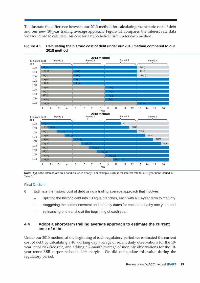
Review of our WACC method IPART 29
To illustrate the difference between our 2013 method for calculating the historic cost of debt
and our new 10-year trailing average approach, Figure 4.1 compares the interest rate data
we would use to calculate this cost for a hypothetical firm under each method.
Figure 4.1 Calculating the historic cost of debt under our 2013 method compared to our
2018 method
2013 method
2018 method
Note: R(y) is the interest rate on a bond issued in Year y. For example, R(0), is the interest rate for a 10-year bond issued in
Year 0.
Final Decision
6 Estimate the historic cost of debt using a trailing average approach that involves:
– splitting the historic debt into 10 equal tranches, each with a 10-year term to maturity
– staggering the commencement and maturity dates for each tranche by one year, and
– refinancing one tranche at the beginning of each year.
4.4 Adopt a short-term trailing average approach to estimate the current cost of debt
Under our 2013 method, at the beginning of each regulatory period we estimated the current
cost of debt by calculating a 40 working day average of recent daily observations for the 10-year tenor risk-free rate, and adding a 2-month average of monthly observations for the 10-
year tenor BBB corporate bond debt margin. We did not update this value during the
regulatory period.
0 4 8 12 16
1
2
3
4
5
6
7
8
9
1010%
10%
10%
10%
10%
10%
10%
10%
10%
10%
% historic debt pool
Period 1 Period 2 Period 3
Year
1 2 3 4 5 6 7 8 9 10 11 12 13 14 15 16
R(1)
R(2)R(-8)
R(-7)
R(-6)
R(-5)
R(-4)
R(-3)
R(-2)
R(-1)
R(0)
R(11)
R(12)
R(8)
R(9)
R(10)
R(3)
R(4)
R(5)
R(6)
R(7)
Period 4
R(13)
0 4 8 12 16
1
2
3
4
5
6
7
8
9
1010%
10%
10%
10%
10%
10%
10%
10%
10%
10%
% historic debt pool
Period 1 Period 2 Period 3
Year
1 2 3 4 5 6 7 8 9 10 11 12 13 14 15 16
R(1)
R(2)R(-8)
R(-7)
R(-6)
R(-5)
R(-4)
R(-3)
R(-2)
R(-1)
R(0)
R(11)
R(12)
R(8,10)
R(9,10)
R(10,10)
R(3,10)
R(4,10)
R(5,10)
R(6,10)
R(7,10)
Period 4
R(13)
R(14)
R(15)
R(16)

30 IPART Review of our WACC method
Our draft decision was to adopt a new approach that involved:
calculating the current cost of debt in line with our 2013 method at the beginning of
each regulatory period
adjusting this estimate at a monthly basis during the regulatory period to reflect changes in the actual cost of debt during the regulatory period, and
making this adjustment at the beginning of the following regulatory period using a
true-up mechanism.
We considered that this would be an incremental improvement to the extent that it
addressed stakeholders’ concerns that the current approach creates refinancing risk, and
enhanced investment incentives because it would reflect the marginal cost of raising debt at
all points during the regulatory period.
4.4.1 Stakeholders did not support our draft decision
Stakeholders were generally receptive of an approach that updates the cost of debt during
the regulatory period, particularly on an annual basis. For example, Hunter Water
suggested that a “well-designed method of updating the current cost of debt should allow the utility to match or closely approximate the actual cost of new debt raised throughout the
regulatory period”.54
However, stakeholders did not support the specific approach we set out in our Draft Report. They identified two particular drawbacks. The first was that it would not reduce
refinancing risk. Because our draft decision resets the current cost of debt estimate at the
beginning of each regulatory period, to match it a firm would still need to refinance at least
half its debt portfolio for a 10-year period just prior to the start of a regulatory period. NSW
Treasury stated:
In order to effectively hedge the current cost of debt allowance, the utility would have to issue all
the debt related to the current cost of debt allowance (50% of total debt portfolio) during the 40 day
averaging period prior to each determination. A pro-rata portion of this debt would mature at each
month-end of the determination period. This maturing debt would then need to be refinanced into
debt that matured at the end of the determination period. The process would then repeat with all
the debt related to the current cost of debt (50% of total debt portfolio) being refinanced. The new
proposal increases the refinancing burden instead of reducing this burden as IPART suggest in
their draft report.55
The second was that updating the current cost of debt on a monthly basis would be
uneconomic. For example, SDP argued that the costs associated with refinancing, or
hedging, a small share of debt each month would be inefficiently high.56 Sydney Water submitted it “would be unlikely for an efficient benchmark entity to refinance
approximately 1 percent of its total debt monthly”.57 However, Sydney Water also thought
the use of monthly data would “provide a fair estimate of efficient debt costs over longer periods relative to say a yearly reference period”.58
54 Hunter Water submission to IPART Draft Report, December 2017, pp 3-4. 55 NSW Treasury submission to IPART Draft Report, December 2017, p 2. 56 SDP submission to IPART Draft Report, December 2017, pp 27-28. 57 Sydney Water submission to IPART Draft Report, December 2017, p 8. 58 Ibid, p 8.

Review of our WACC method IPART 31
Several stakeholders proposed that, if we maintain the midpoint rule, we could instead
update the current cost of debt by adopting a short-term trailing average approach, on the
basis that this would be an incremental improvement over our 2013 method.59 In contrast,
SDP proposed we update the current cost of debt by re-estimating the current cost of debt on an annual basis, by:
[resetting] the current cost of debt allowance each year in a defined 40 day window of time just
prior to the commencement of the year in which prices are changed (rather than each month, as
proposed by IPART in the Draft Report). This would ensure that an efficient business can match
reasonably closely the cost of debt associated with its short-term debt pool, whilst exposing
businesses to the prevailing cost of debt and efficient investment signals.60
Figure 4.2 illustrates how SDP’s approach would work for a firm with a 4-year regulatory period.
Figure 4.2 How SDP’s proposed approach to estimating the current cost of debt would
work
Note: R(y, T) is the interest rate on a bond issued in Year y for a term of length T. For example, R(0,10), is the interest rate for
a 10-year bond issued in Year 0.
4.4.2 We will adopt a short-term trailing average approach for the current cost of
debt
We agree with stakeholders on the two drawbacks they identified with our draft decision, and with the suggestion that updating the current cost of debt by adopting a short-term
trailing average approach would be an incremental improvement over our 2013 method.
We are concerned that SDP’s proposed approach would result in excessive price volatility. Figure 4.3 plots the absolute annual changes in the risk-free rate and the debt margin, since
2006. It shows that SDP’s proposed approach could lead to significant annual movements in
interest rates.
Accordingly, our final decision is that we will estimate the current cost of debt as a short-
term trailing average.
59 WaterNSW submission to IPART Draft Report, December 2017. pp 13-14, Sydney Water submission to
IPART Draft Report, December 2017, p 8, Hunter Water submission to IPART Draft Report, pp 3-4 and NSW Treasury submission to IPART Draft Report, December 2017, p 3.
60 SDP submission to IPART Draft Report, December 2017, p 5.
0 1 2 3 4 5 6 7 8
1
2
3
4
1 2 3 4 5 6 7 8
Period 1 Period 2% of current debt pool
Year
25%
25%
25%
25%
R(1,10)
R(1,10)
R(1,10)
R(2,10)
R(2,10) R(3,10)
R(1,10) R(2,10) R(3,10) R(4,10)
R(2,10) R(3,10) R(4,10) R(5,10)
R(3,10) R(4,10) R(5,10) R(6,10)
R(4,10) R(5,10) R(6,10) R(7,10)
R(5,10)
R(6,10)
R(8,10)
R(7,10)
R(6,10) R(7,10) R(8,10)
R(7,10) R(8,10)
R(8,10)

32 IPART Review of our WACC method
Figure 4.3 Absolute annual changes in the risk-free rate and debt margin
Note: Each point calculates the annual change in the risk-free rate and debt margin, with the risk-free rate and debt margin
measured over a 40-day, or 2-month period, in the two years.
Data source: Bloomberg; RBA
4.4.3 We will estimate the short-term trailing average by splitting the current cost
into tranches
Under the 2018 method, we will estimate the short-term trailing average in a similar way to
the 10-year trailing average. We will split the current cost of debt into a number of equal
tranches. This number will be equal to the years in the regulatory period, and the commencement and maturity dates for each tranche will be staggered by one year.61 At the
start of each year of the regulatory period, the oldest tranche of debt will mature and a new
tranche at the new prevailing interest rate will replace it.
Once the short-term trailing average is fully implemented, it will measure the average cost
over a period equal in length to the regulatory period. For example, over a 4-year regulatory
period, it will measure the average cost of debt over the previous four years.
To update the current cost of debt, we will calculate the change in the current cost of debt
each year during the regulatory period by:
measuring the interest rate of the new tranche of debt, and subtracting the interest rate of the maturing tranche of debt, and
dividing this number by the total number of tranches (eg, four).
We will account for any changes to the length of the regulatory period as they arise, usually
as part of the review process.
We will adopt the same approach to measure the interest rate for each annual tranche of
debt for both current and historic estimates (ie, adopting a consistent 40-day period that we will choose). See section 4.5 for further explanation.
61 This differs from the approach to estimating the current cost of debt we proposed in our Draft Report. The
method in our Draft Report staggered the commencement dates, but did not stagger the maturity dates, for each tranche of debt.
0
100
200
300
400
500
600
700
2006 2008 2010 2012 2014 2016
Risk free rate
Debt risk premium
Bps

Review of our WACC method IPART 33
We will also adopt a 10-year term-to-maturity (TTM) for the current estimate of the cost of
debt. See section 4.8 for further explanation.
4.4.4 We will transition to the short-term trailing average over one regulatory period
Unlike the historic cost of debt, our 2013 and 2018 methods for estimating the current cost of
debt are distinctly different. Our 2013 method measures the cost of debt at a discrete 40
working day window each regulatory period, whereas the short-term trailing average measures the average cost of debt over a period equal in length to the regulatory period.
Given this difference, we have decided to transition to the new method, to promote stability
and to allow stakeholders sufficient time to transition to our new method.
At the beginning of the next regulatory period when our new WACC method applies, we
will initially set the current cost of debt as a 40-day average, in line with our 2013 method.
At the beginning of the second year, we will begin updating the current cost of debt, by
taking the average across the interest rates in each tranche of debt, as shown in Figure 4.1.
We will calculate the change in the cost of debt at the beginning of Years 2 to 4 of the period
(ΔRi), as:
Δ𝑅𝑖 =(𝑅𝑖−𝑅1)
4(2)
where Ri is the interest rate in year i=2,3,4.
We will pass through this change in the 10-year trailing average to prices with an annual
update, or via a regulatory true-up in the following period.
To illustrate the difference between our 2013 method for calculating the current cost of debt
and our new short-term trailing average approach, Figure 4.4 compares the interest rate data
we would use to calculate this cost for a hypothetical firm under each method.

34 IPART Review of our WACC method
Figure 4.4 Calculating the current cost of debt under our 2013 method and 2018 method
2013 method
2018 method
Note: R(y) is the interest rate on a bond issued in Year y. For example, R(0), is the interest rate for a 10-year bond issued in
Year 0.
4.4.5 Our 2018 method for estimating the current cost of debt is an incremental
improvement
We are satisfied that adopting a short-term trailing average for the current cost of debt is an incremental improvement over our 2013 method. Compared to the 2013 method, our new
method increases accuracy, reduces refinancing risk for firms and maintains efficient
investment incentives. These benefits more than offset the slight increase in complexity.
Increases accuracy
Our new method measures the cost of debt in each year of the regulatory period, whereas the 2013 method measures the cost of debt in a 40-day period before the beginning of each
regulatory period. Therefore, our 2018 method will more accurately account for changes in
the cost of debt over time.
Reduces refinancing risk
Under our 2013 method, a firm that issues long-term debt gradually (eg, on a staggered maturity basis) can face significant refinancing risk. The firm can contract interest rate
swaps over the 40 working day period prior to the beginning of the regulatory period to
0 1 2 3 4 5 6 7 8
1
2
3
4
1 2 3 4 5 6 7 8
Period 1 (transition) Period 2% of current debt pool
Year
25%
25%
25%
25%
R(1)
R(1)
R(1)
R(1)
R(1) R(1)
R(1) R(1) R(1) R(1)
R(1) R(1) R(1) R(5)
R(1) R(1) R(5) R(5)
R(1) R(5) R(5) R(5)
R(5)
R(5)
R(5)
R(5)
R(5) R(5) R(5)
R(5) R(5)
R(5)
0 1 2 3 4 5 6 7 8
1
2
3
4
1 2 3 4 5 6 7 8
Period 1 (transition) Period 2% of current debt pool
Year
25%
25%
25%
25%
R(1)
R(1)
R(1)
R(1)
R(1) R(1)
R(1) R(2) R(2) R(2)
R(1) R(3) R(3) R(3)
R(1) R(4) R(4) R(4)
R(1) R(5) R(5) R(5)
R(2)
R(3)
R(5)
R(4)
R(6) R(6) R(6)
R(7) R(7)
R(8)
Review of our WACC method IPART 35
match the risk-free rate. However, there can be a large mismatch between the debt margin,
measured over a 2-month period prior to the beginning of the regulatory period, and their
actual debt margin, which is an average across their outstanding debt issuance.
Our 2018 method significantly reduces this risk. This is because the mismatch between the debt margin is smaller, because our 2018 method samples the debt margin over a regulatory
period (typically 3-5 years). The firm can still contract interest rate swaps, each year on a
rolling basis, to hedge changes in the risk-free rate.
That said, under the short-term trailing average, the firm would not typically match the
average debt margin across their outstanding debt issuance in a given regulatory period.
However, over the course of multiple regulatory periods, the short-term trailing average should approximate the firms’ actual debt margin. This is because the short-term trailing
average is a short-term moving average, whereas the firm’s actual debt margin would be a
long-term moving average. In some regulatory periods, the short-term average will be higher than the long-term average, but in other periods it will be lower.
In contrast, under our 2013 method, a firm issuing long-term debt would not be able to
match the current estimate of the debt margin, even across many regulatory periods. This is because we estimated our current debt margin at discrete points in time, rather than as a
short-term average.
Maintains efficient investment incentives
To provide efficient investment signals, our estimate of the current cost of debt should
reflect the marginal, or current, cost of borrowing. Our 2013 method, and the short-term trailing average, equally reflect the marginal cost of financing new investment. To see why,
consider a firm with a 4-year regulatory period:
Under our 2013 method, at the beginning of the period the current cost of debt is the marginal cost of borrowing. By the end of the period, the estimate is four years out of
date. Over the course of the regulatory period, the cost of debt estimate is two years
out of date on average.
Once implemented, our 2018 method measures the average cost of debt over the past
four years at all points during the regulatory period. In effect, the average of this
window is a cost of debt estimate that is two years out of date.
Slightly increases complexity
Our new approach does increase the complexity of our 2018 method, because we have to
pass through changes in the cost of debt, either through an annual update or using a
regulatory true-up in the following period. For the current cost of debt, we will transition to
our new method over one regulatory period.
However, we consider that this increase in complexity is modest. We have clearly outlined
how we pass through changes in the cost of debt under the two options, and the transition to
the short-term trailing average is straightforward and occurs within a single regulatory period.
Overall, we consider that the reduction in refinancing risks under our proposed approach is
material, and sufficient to warrant the increased complexity of a short-term trailing average.

36 IPART Review of our WACC method
Final Decision
7 Estimate the current cost of debt using a short-term trailing average approach that
involves:
– splitting the current debt into tranches equalling the number of years in the regulatory
period, each with a 10-year term to maturity, and
– staggering the commencement and maturity dates for each tranche so that at the
beginning of each year of the regulatory period, the interest rate on the oldest
tranche of debt will reprice at the prevailing interest rate on the new tranche of debt.
4.5 Adopt consistent observation windows in calculating historic and current costs
We estimate both the historic and current cost of debt by observing market interest rates and
debt risk premia. Under our 2013 method, we observe:
The current cost of debt over a window of 40 working days close to the start of the regulatory period. We take the average of 40 daily observations to sample the risk-free
rate, and the average debt risk premium over a similar window.
The historic cost of debt over a window of 10 years. We take the average of all daily observations over approximately 2,500 working days for the risk-free rate, and the
debt risk premium over a matching window, taking the average over 120 monthly
observations.
We have decided to maintain the 40-day observation window for current debt. This
window will apply each year when we update the trailing average for the current cost of
debt. We will inform only the regulated firm of the exact timing of this observation window in advance so it can make efficient hedging arrangements without signalling to the market a
large debt issuance, which might potentially distort the price. This position on the
observation window is consistent with our Draft Report.
We have also decided to change the observation window for historic debt so it is consistent
with that for current debt. Instead of a 10-year daily average, we will average 10 annual
observations. Each annual observation will be the average across a 40-day observation window. We will inform the regulated firm of the exact timing of the observation window
for the current year on a confidential basis in advance. Observation periods for past years
will remain fixed. This is a change since our Draft Report.
The observation windows for current and historic debt will be consistent for each annual
tranche.
4.5.1 Stakeholders were divided on observation window
In further consultations with stakeholders, stakeholders were divided on their preferred
observation window. On one hand, SDP preferred a continuation of the 40-day observation window that we use now for current debt, because it is more efficient for a debt issuer of its
size to go to market infrequently with debt tranches of a certain minimum size.62 An
62 Consultation between IPART and stakeholders, January 2018.

Review of our WACC method IPART 37
observation window longer than 40 working days would lead to an average cost of debt that
it would be unable to replicate in the market, given its current issuing practices.
On the other hand, TCorp suggested that we move to an observation window similar to that
used by the AER.63 Under the AER’s approach, each regulated firm would nominate its own preferred dates and length of observation window in advance. The window may be as
short as 10 working days or as long as one year, at the firm’s discretion.64 Treasury and
TCorp’s reasons for moving to such an approach appeared to be that:
As they borrowed for all of the NSW Government’s requirements it was a practical
necessity to tap bond markets frequently during the year.
If TCorp and the state-owned utilities were to align the fund-raising activity to the 40-day observation window, TCorp could saturate the market with debt raising. This
saturation would increase the Government’s cost of borrowing.65
4.5.2 We will use a 40-day sampling period in our 2018 method
In our view, we should not employ different observation windows for different regulated
firms, as this would potentially lead to different WACC results for otherwise similar organisations. That means the length of the observation window must be the same for all
the firms we regulate. It also means that when we set prices for two firms at the same time,
the observation windows should be the same.
We agree with SDP’s reasoning in support of continuing to use a 40-day period. We have
considered the arguments TCorp put to us, but have decided not to allow firms to choose
the timing or the length of the observation window.
While TCorp needs to issue debt on a continuous basis, part of the reason for this is that it
needs to issue debt to service a whole-of-government portfolio. Firms in a competitive
market do not tend to issue debt continuously; they would only do so at various points in time.
In addition, under our 2018 method the short-term trailing average cost of current debt
consists of annual tranches of debt with a 10-year term-to-maturity. Most stakeholders indicated to us that they would not actually refinance each of these tranches each year.
Instead they would hold tranches of long-term debt (eg, 10-year tenor) that are refinanced
less frequently, and use swap contracts to match the regulatory debt allowance. If stakeholders refinance swap contracts each year, TCorp’s concerns should be addressed if
we do not publicly disclose the observation window ahead of time.
Final Decisions
8 For the current cost of debt, maintain a 40-working day observation window for the risk-
free rate and an equivalent two-month observation window for the debt risk premium and:
– choose the exact timing of the observation window
– inform the regulated firm in advance on a confidential basis.
63 Ibid. 64 Australian Energy Regulator, Better Regulation, Rate of Return Guideline, December 2013, p 4. 65 Consultation between IPART and stakeholders, January 2018.

38 IPART Review of our WACC method
9 For the historic cost of debt, adopt a 40-working day observation window for the risk-free
rate and an equivalent two-month observation window for the debt risk premium for each
new point in the trailing average calculation and:
– choose the exact timing of the observation window
– inform the regulated firm in advance on a confidential basis.
4.6 Decide how to pass-through annual changes
Under our new trailing average approaches for estimating the historic and current costs of debt, we need to update our decision on the cost of debt each year. We considered whether:
prices should update each year to reflect the updated cost of debt, or
the regulated business should store the price changes until the start of the next regulatory period, when we would implement them through an NPV-neutral true-up
to the regulatory revenue requirement.
In our view, each option should be equivalent in present value terms, so the decision to take one approach or the other should have no impact on the value of a regulated firm. Likewise,
the effect on the firm’s customers should also be equivalent in present value terms.
Therefore we will decide whether to apply annual price adjustments or a true-up on a case-by-case basis, as part of our review process. In making this decision, we will have regard to
any evidence the regulated firm or its customers put forward to support one approach or the
other. Neither option would be a default.
This final decision differs from our draft decision, which was to use an end-of-period true-
up for all firms.
4.6.1 Stakeholders expressed mixed views on the options
SDP and WaterNSW submitted their strong preferences for annual price adjustments to
reflect changes to interest costs.66 For example, SDP noted that while a firm was waiting to receive a true-up in its favour in several years’ time, it could potentially breach its debt
covenants, which often specify financial ratios that must be met in each year.67 While the
eventual receipt of the true-up would theoretically overcome the problem, it might not be timely from the lenders’ point of view.
On the other hand, Sydney Water submitted its strong preference for using a true-up to
adjust prices. It stated that “the benefits to our customers of simple, transparent and stable bills for the entire regulatory period far outweighs any perceived small cumulative benefits
of unidirectional changes in bills over the regulatory period”.68
66 SDP submission to IPART Draft Report, December 2017, pp 8-10; WaterNSW submission to IPART Draft
Report, December 2017, p 9. 67 SDP submission to IPART Draft Report, December 2017, p 9. 68 Sydney Water submission to IPART Draft Report, December 2017, p 2.
Review of our WACC method IPART 39
4.6.2 We will decide between annual price changes or true-up as part of our
determination
We can see merit in both points of view. The different perspectives reflect the different
circumstances of each organisation. For this reason, we have decided not to impose a
uniform rule on all regulated firms. Instead, we will decide whether to apply annual price adjustments or the true-up on a case-by-case basis, as part of our review process. In
reaching this decision, we will consider any submissions from the regulated business, its
customers and other relevant stakeholders. Neither option would be considered the default.
Final Decision
10 Update the regulatory cost of debt annually, and decide whether to pass through changes
via annual price adjustments or a true-up in the subsequent period:
– as part of the price determination, and
– on a firm-by-firm basis.
4.7 Where we use a true-up we will discount changes by the WACC
Where we determine that we will use the true-up for a regulated firm, we must use a
discount rate in the present value calculations. We have decided that we will apply the
firm’s regulatory WACC as the discount rate that we will use in the true-up calculation.
4.7.1 One stakeholder advocated the cost of debt as the discount rate
While it did not comment in submission to the Draft Report, TCorp noted in consultations that the firm’s cost of borrowing should be the discount rate. It argued that only that rate
would preserve the par value of the interest rate changes when the true-up was paid.69
4.7.2 We will use the WACC as the discount rate
The true-up is a cash asset or liability of the regulated firm, depending on whether it is paid
to the firm or by it. If it is an asset, then it could be used to avoid the need to raise additional funds for capital investments. The opportunity cost of those additional funds is the firm’s
regulatory WACC.
If it is a liability then it must be funded by raising additional capital. That would involve additional borrowing. However, if it is funded entirely by borrowing that would have the
effect of altering the firm’s gearing ratio. In order to maintain the current gearing ratio,
which is the gearing ratio of an efficient benchmark firm, the firm would need to raise additional equity as well. The average cost of capital the firm would face to do this would
be its regulatory WACC.
For this reason, the discount rate used in the true-up calculation should be the firm’s regulatory WACC.
69 Consultations between IPART and TCorp, January 2018.

40 IPART Review of our WACC method
Final Decision
11 Where a true-up is used to pass through changes in the cost of debt, the discount rate
used to calculate the true-up amount will be the firm’s regulatory WACC.
4.8 Annualise bond yield data
In Australia, government and corporate bond yields are typically derived from semi-annual
rates of return.70 In other words, risk-free rates are based on semi-annual rates of return,
and we assume that the RBA data we use to estimate the debt margin is also based on semi-annual rates of return. We currently calculate the average annual rate of return for a 10-year
government bond (the yield to maturity) by simply doubling the rate of return that an
investor would earn over half a year.
However, this ignores the impact of compounding on investment returns. Figure 4.5
illustrates the impact that adjusting annual rates of return for compounding would have on
our cost of debt estimates. For example, if the cost of debt was 6% using semi-annual rates, the annualised rate of return would be 6.09%.
Figure 4.5 Effect of converting semi-annual yields to annualised yields (%)
Other regulators, including the AER, ERAWA and QCA, convert published yields into an effective annual rate.71 Our draft decision was to adopt this same approach. All
stakeholders who commented supported our draft decision.72
Therefore, our final decision is to convert published bond yield data into annualised yields, using the proposed method in Box 4.1.
70 Quoting the yield to maturity based on semi-annual rates of return is standard bond market convention in
Australia. This is because AGS bonds typically pay interest every six months. For more details, see AFMA, Long Term Government Debt Securities Conventions, January 2017, p 4.
71 AER, Better Regulation, Rate of Return Guideline, December 2013; Economic Regulation Authority, Determination on the 2016 Weighted Average Cost of Capital for the Freight and Urban Railway Networks, and for the Pilbara railways, October 2016; Queensland Competition Authority, Final decision, Trailing average cost of debt, April 2015; Queensland Competition Authority, Cost of capital: market parameters, August 2014.
72 Hunter Water submission to Draft Report, December 2017, p 9; Sydney Water submission to IPART Draft Report, December 2017, p 4; SDP submission to IPART Draft Report, December 2017, p 13.
0
2
4
6
8
10
12%
Cost of debt (annualised)Cost of debt (semi-annual)
Review of our WACC method IPART 41
Box 4.1 Proposed method for annualising bond yield data
As outlined above, government and corporate bond yields are typically derived from semi-annual
rates of return.
If the rate of return based on semi-annual yields is ys, then the annualised rate of return, ya, would
be calculated as follows in equation (1) below:
𝑦𝑎 = (1 +𝑦𝑠
2)
2− 1 (3)
We propose to adjust our cost of debt by the following factor, Δd
∆𝑑= (1 +(𝑦𝑅𝐹+𝑦𝐷𝑅𝑃)
2)
2
− (1 + 𝑦𝑅𝐹 + 𝑦𝐷𝑅𝑃) (4)
where 𝑦𝑅𝐹 and 𝑦𝐷𝑅𝑃 are the published risk-free rate and debt margin.
The risk-free rate also enters into the calculation of the cost of equity, which we propose to adjust
by the factor Δe
∆𝑒= (1 +𝑦𝑅𝐹
2)
2− (1 + 𝑦𝑅𝐹) (5)
Final Decision
12 Convert published bond yield data into annualised yields.
4.9 Maintain a 10-year term-to-maturity
We currently use a 10-year term-to-maturity (TTM) to estimate the cost of debt under our
2013 method, and our draft decision was to maintain this approach. All stakeholders who provided commented on this issue supported our draft decision.73
We consider a 10-year TTM is appropriate for all industries we regulate because:
adopting a shorter TTM may encourage firms to issue short-term debt to fund long-term assets
the efficient cost of finance for an asset is the cost of financing the asset over its life,
and the firms we regulate tend to have long lived assets
there is broad evidence that firms operating long-lived assets seek to raise debt with a
maturity of 10 years or longer, and
there are benefits in adopting a single TTM for all industries.
At the same time, we recognise that estimating the current cost of debt as a short-term
trailing average and assuming a 10-year TTM creates a mismatch between the timing of
when the interest rate on debt is repriced, and how frequently underlying debt is refinanced.
73 Hunter Water submission to Draft Report, December 2017, p 9; Sydney Water submission to IPART Draft
Report, December 2017, p 4; SDP submission to IPART Draft Report, December 2017, p 13.

42 IPART Review of our WACC method
With a short-term trailing average, the interest rate applied to each tranche of debt is
assumed to reprice every 3-5 years in line with the length of the regulatory period. To match
the repricing risk of our current cost of debt estimate, a firm with a 4-year regulatory period
could simply issue 4-year debt on a rolling basis.
However, we have decided to maintain a 10-year TTM to estimate the current cost of debt as
our analysis suggests that the firms we regulate should issue long-term debt, and because
firms can manage the repricing mismatch through interest rate swaps. Box 4.2 presents analysis supporting our final decision.

Review of our WACC method IPART 43
Box 4.2 Our analysis supports a 10-year term to maturity
A 10-year term-to-maturity encourages long-term borrowing
We consider that using 10-year bond yields to estimate the cost of debt is more appropriate than
using short-term bond yields because almost all regulated firms that we set a WACC for operate
assets with long lives. As outlined in our Issues Paper, to the extent that regulated firms operate
assets with long lives, they would be exposed to refinancing risk if they did not issue long-term
debt.a
In addition, it is inefficient if the TTM we assume does not match the life of the firms’ assets. The
efficient cost of finance for an asset is the cost of financing the asset over its life. As we noted in
our 2013 review:
The real asset is the underlying physical assets, which generate the cash flow over their expected
economic lives…Investors seeking to invest in a utility, whether regulated or unregulated, would value the
business based on the expected cash flow that would be generated by the business over the expected life
of its assets.b
Therefore, the TTM we assume for the firm should as closely as possible reflect the average life of
its assets. For example, using a 5-year TTM may be inefficient relative to a 10-year TTM for assets
with long lives.
Firms operating long-lived assets raise long-term debt
There is also broad evidence that firms operating long-lived assets seek to raise debt with a
maturity of 10 years or longer. Figure 4.6 shows a sample of domestic businesses investing in
long-lived assets issue bonds with a maturity of 10 years or longer.
Figure 4.6 Bond maturity profile for a sample of domestic businesses (years)
Note: This figure presents the average maturity of bonds on an ‘original maturity’ basis (the maturity of the bond at issue).
Data source: Bloomberg.
0
5
10
15
20
25
30
AGL APT piplines BHP Sydney Airport Weighted average
Ave
rag
e m
atu
rity
at is
su
an
ce
(ye
ars
)

44 IPART Review of our WACC method
There are practical benefits in setting a single TTM for all industries
In principle, the TTM we use to set the WACC for a business should reflect an average asset life
for the industry. That is, if we set a WACC for a firm operating in an industry which invested in
short-lived assets, then it would be more efficient to set the WACC based on short-term bond
yields. This would suggest the TTM should vary by industry.
In practice, we consider that using a 10-year TTM for all industries is more appropriate than
determining industry-specific TTMs:
Almost all regulated firms that we set a WACC for operate assets with long lives, of at least
10 years on average.
The 10-year cost of debt can be measured reliably over time.
A single TTM results in a simpler, more consistent approach, and reduces parameter
uncertainty for the businesses that we regulate.
a IPART, Review of our WACC Method – Issues Paper, July 2017, p 25.
b Ibid, p 11.
c Ideally we would match the TTM to the asset lives. However, in practice the debt market does not offer products to
exactly match the asset lives for long-lived infrastructure assets.
Final Decision
13 Continue to use a 10-year term to maturity to estimate the cost of debt.
4.10 Continue to use 10-year coupon paying bond yields
To measure the cost of debt, under our 2013 method we use bond yield data for coupon-
paying bonds that mature in approximately 10 years’ time. For example, our 2013 method to estimate the risk-free rate of return is to use the yield of an Australian Government bond,
maturing in approximately 10 years’ time, which pays interest every six months (ie, semi-
annual coupons).
This approach closely approximates the cost of borrowing for 10 years, although it is not
conceptually equivalent to the true cost of borrowing for 10 years. This is because an
investor who purchases this bond receives a series of cash payments every six months over a 10-year period. The interest rate risk associated with a 10-year government bond is a
combination of the 10-year interest rate, which applies to the principal payment and final
coupon payment, and the rates of return applying to the other coupons paid over the life of the bond.74
To estimate the interest rate risk of borrowing over a 10-year period, we could calculate a
‘zero-coupon’ bond yield using bond market data.75 The RBA publishes risk-free rates based on zero-coupon yields on a daily frequency on the second business day of each
month. However, to do this, the RBA uses coupon-bearing bonds to estimate zero-coupon
bond prices using a modified Merrill Lynch Exponential Spline methodology.76
74 RBA, Extracting Information from Financial Market Instruments, RBA Bulletin, March Quarter 2012. 75 Nominal yields for Australian Government Bonds are adjusted for coupon payments to derive their zero
coupon yields. See RBA, Extracting Information from Financial Market Instruments, RBA Bulletin, March Quarter 2012.
76 For more details, see Finlay and Chambers, A Term Structure Decomposition of the Australian Yield Curve, RBA Research Discussion Paper, December 2008.
Review of our WACC method IPART 45
While our 2013 method is not identical to the true cost of borrowing for 10 years, it is
transparent, replicable and results in an accurate proxy of borrowing costs. We consider
that this is important, and therefore our draft decision was to continuing using published
coupon-paying bond yield data.
As all stakeholders who commented supported our draft decision,77 our final decision is to
continue to use 10-year coupon paying bond yields in our 2018 method.
Final Decision
14 Continue to use the 10-year coupon-paying bond yield data to estimate the cost of debt.
4.11 Continue to use the BBB debt margin published by the RBA
To estimate the debt margin, we currently use estimates published by the RBA of the spread between the yield of BBB-rated bonds issued by Australian non-financial corporations to
AGS yields.78 They are an aggregate of spreads for bonds issued with BBB+, BBB, and BBB-
credit ratings, with a residual maturity close to the target 10-year tenor.79
Our draft decision was to continue to use the BBB debt margin published by the RBA
because:
We found that the BBB credit rating is generally the most appropriate measure of the debt margin for a benchmark firm operating in a competitive market, even if the firms
we regulate might not be BBB rated.
The RBA data is our preferred data source for estimating the debt margin.
The analysis we considered in making this decision is outlined in Box 4.3.
All stakeholders who commented supported our draft decision.80 Therefore, our final
decision is to continue to use the BBB debt margin published by the RBA in our 2018 method.
Box 4.3 Our analysis supports using the RBA’s estimate of the BBB debt margin
In deciding how to estimate the debt margin, we addressed the following three issues:
1. Whether we adopt a single credit rating for all industries, or estimate a different credit rating in
each industry for which we set prices.
2. If we continue to adopt a single credit rating across industries, whether the BBB rating is the
most appropriate credit rating.
3. Whether we continue to calculate the debt margin using the RBA’s measure of corporate debt
spreads.
77 Hunter Water submission to Draft Report, December 2017, p 9; Sydney Water submission to IPART Draft
Report, December 2017, p 4; SDP submission to IPART Draft Report, December 2017, p 13. 78 See: IPART, Fact Sheet: New Approach to Estimating the Cost of Debt: Use of the RBA’s Corporate Credit
Spreads, February 2014. 79 For further information about how bonds are chosen as part of the RBA’s estimates, please see: Arsov, et
al, New Measures of Australian Corporate Credit Spreads, RBA Bulletin Article, December Quarter 2013, pp 15-26.
80 Hunter Water submission to Draft Report, December 2017, p 9; Sydney Water submission to IPART Draft Report, December 2017, p 4; SDP submission to IPART Draft Report, December 2017, p 13.

46 IPART Review of our WACC method
It is practical to adopt a single credit rating for all industries
In principle, the credit rating we use to estimate the debt margin should vary, to some extent, by
industry. For example, some industries operate in more stable markets than others, and therefore
the risks of investing in those industries could be lower both for debt and equity investments.
In practice, it is not feasible to estimate a benchmark industry credit rating accurately. For
example, to estimate an industry credit rating, we might look to use the proxy firms we currently
use to estimate equity beta (and the gearing ratio). However there are at least two reasons why
this is difficult to do in practice.
4. In many industries, only a small proportion of these proxy firms has received a credit rating
from a ratings agency, and therefore may not be representative of an average across the
industry.
5. Most of the proxy firms are foreign-based. The credit ratings for these firms are often not
directly comparable to an equivalent firm operating in Australia. A BBB-rated proxy firm
operating in a country where sovereign government debt has a BBB credit rating is unlikely to
have the same risk profile as a BBB-rated firm operating in Australia (where sovereign debt is
AAA-rated).
Therefore, we have decided to adopt a single credit rating for all industries we regulate.
A BBB credit rating is most appropriate
We consider that the BBB credit rating is most appropriate because we consider that the BBB
rating will, on average, provide an efficient estimate of the WACC. We can adjust the gearing ratio
for individual firms because the gearing ratio and the credit rating are endogenous.a A credit rating
higher than BBB would mean the benchmark firm would need to rely on a higher proportion of
relatively expensive equity. Conversely, if the benchmark firm was sub-investment grade, the
increase in the debt margin would likely more than offset the reduction in equity costs.
We prefer the RBA data, to other data sources, to measure the BBB debt margin
We have decided we will continue to use only the RBA data. It is our preferred data source
because we consider the estimates are reliable, it is publicly available, and the RBA has published
its methodology for calculating the debt margin.b Alternative measures of the debt margin are
currently available only with a paid subscription to these services, which would make it more
expensive for stakeholders to replicate our method.
If the RBA should stop publishing this series, we could consider these alternatives, or calculate the
debt margin ourselves by applying the RBA’s published methodology to current market data.
a For example, if a water utility has a credit rating of A or AA, then it is probably under-geared. It could borrow more,
reducing its rating as far as BBB while remaining investment grade. Doing so could reduce its cost of capital, since it would
need to rely on a smaller proportion of relatively expensive equity in its capital structure.
b Arsov, Brooks and Kosev, New Measures of Australian Corporate Credit Spreads, RBA Bulletin Article, December
Quarter 2013, pp 15-26.
Final Decision
15 Continue to use the 10-year BBB corporate bond spreads published by the RBA to
measure the debt margin across all industries.
Review of our WACC method IPART 47
5 Determining the cost of equity
Under our 2013 WACC method, we use a Capital Asset Pricing Model (CAPM) to estimate the cost of equity. Under this model, the cost of equity equals the sum of the risk-free rate of
return and the product of the market risk premium (MRP) and the equity beta.
Like most regulators in Australia and overseas, we use the Sharpe-Lintner CAPM (SL-CAPM). In applying this model, we estimate the current cost of equity and the historic cost
of equity and select the midpoint value. This involves:
estimating a historic and a current risk-free rate (as discussed in Chapter 4)
estimating a historic and a current MRP, and
estimating equity beta and gearing levels using a selection of proxy companies when
we first estimate a benchmark WACC for a regulated industry, and reviewing this value in subsequent reviews.
As part of the review, we considered a range of refinements to this approach and the
measures we use. The sections below provide an overview of our final decisions and then discuss them in detail.
5.1 Overview of final decisions on cost of equity
We have decided to continue to use the SL-CAPM, as there is not a sufficient case to replace it with an alternative model. However, we will monitor the impact that moving to the
Fama-French model would have on our WACC decisions over the next five years.
We have also decided to continue to determine the cost of equity as the midpoint between our estimates of the current and historic cost of equity at the start of the regulatory period,
and to not update this cost during the regulatory period. And we will continue to measure
the historic MRP as a range with a midpoint of 6%.
However, we will modify our approach and measures for estimating the current MRP.
While we will still estimate this value using six different methods and then select a single
point estimate, we will modify one of the methods – the market indicator method – by
replacing two of the indicators we currently use (the dividend yield and the risk-free rate)
with a single new indicator (earnings yield less the risk-free rate.
We will also modify the way we select a single point estimate for the current MRP so we:
combine the estimates derived by the five dividend discount model (DDM) methods
into a single DDM MRP by calculating the median estimate, and
calculate the weighted average of this median DDM MRP and the market indicator MRP, giving a two-third weight to the former and a one-third weight to the latter.

48 IPART Review of our WACC method
Further, we will modify our approach and measures for estimating the equity beta. We will
continue to re-estimate this value at each price review in order to engage effectively and
transparently with all interested parties. However, we will only change the value we use in
our WACC calculations where we consider there is sufficient evidence to support this. In addition, we will:
use the broadest possible selection, but exclude thinly traded stocks to improve our
selection of proxy companies
amend our proxy selection process to make it more transparent, predictable and
replicable for stakeholders
continue to use the Vasicek adjustment, but no longer use the Blume adjustment to refine our approach to mitigating estimation bias in raw OLS beta estimates.
These decisions are consistent with our draft decisions, but we have made an additional
decision to amend our proxy selection process in response to stakeholder feedback.
5.2 Continue to use the Sharpe-Lintner CAPM
We currently use the SL-CAPM to calculate the cost of equity. According to this model, only
systematic risk affects the expected return required by the marginal equity investor (who determines the price of equity). This is because the marginal investor would hold a well-
diversified portfolio of equities, and a diversification strategy can remove firm-specific risk.
The average cost of equity across the entire market comprises a risk-free rate (representing the rate an investor would receive for zero risk to their capital) plus a premium that reflects
the additional systematic risk a marginal equity investor bears (representing the average
premium the investor would be willing to accept for a less-than-certain return). This is premium is known as the MRP.
Movements in the stock market affect some firms more than others. For example, utility
firms that offer essential services tend to maintain a fairly steady profit margin through market upturns and downturns because there is a relatively steady demand for these
services. On the other hand, firms that offer discretionary consumer products, especially
luxury items, tend to be highly exposed to market dynamics.
We capture this varying sensitivity to the state of the market through a firm-specific
parameter called the equity beta (βe):
An equity beta of one implies that the firm’s rate of return (ie, after-tax profits divided
by the value of equity) is the same as for the market as a whole at each point in time.
That does not mean that the firm’s rate of return is constant – rather it varies at the
same time and in the same way as the overall market rate of return.
An equity beta below one implies that the firm’s rate of return is less sensitive to
upturns and downturns than the market overall.
An equity beta above one implies that the firm’s rate of return is more sensitive to upturns and downturns than the market overall.
Given these points, the SL-CAPM states that:
Review of our WACC method IPART 49
Expected rate of return on equity = risk-free rate + MRP x βe (6)
5.2.1 One stakeholder submitted that we should use an alternative model
Notwithstanding regulators’ widespread use of the SL-CAPM, academic research indicates that it tends to underestimate the cost of equity for low-equity beta stocks (such as regulated
natural monopoly firms).
To address this downward bias, Sydney Water submitted that we use an alternative model to the SL-CAPM to address this downward bias.81 It stated:
In its 2013 Draft Determination, IPART expressed a view that the Sharpe CAPM used may exhibit
a degree of downward bias and agreed corrective measures are required. This view is in line with
views expressed by the Australian Energy Regulator (AER) on this issue and was supported by
Sydney Water.
However, from our observations of IPART’s historical WACC estimates since 2014, it is unclear if
IPART has applied any corrective remedies discussed in its 2013 Draft Determination. As a basic
principle Sydney Water seeks ongoing commitment from IPART to use alternative CAPMs such
the Fama French, Black or Sharpe-Lintner models to address the acknowledged downward bias of
the Sharpe CAPM.82
5.2.2 Our analysis for our Draft Report found insufficient evidence to support an
alternative model
In our view, it is prudent to periodically assess whether the SL-CAPM is the most appropriate pricing model for our WACC method. We agree that other models may exhibit
less bias than the SL-CAPM. However, there may be theoretical or practical reasons not to
use them. We consider that we should only change the asset pricing model we use in estimating the cost of equity where:
the alternative model more accurately estimates the cost of capital
the alternative model produces results that are stable over time to give stakeholders certainty
the alternative model produces results that are predictable, transparent and reduce
resources required for each review, and
we receive sufficient evidence that changing to the alternative model would increase
the accuracy of our WACC estimates.
For our Draft Report, we assessed two alternatives pricing models – the Black CAPM and the Fama-French model. Our analysis (which is summarised in Appendix C) found
insufficient evidence to suggest either alternative would be superior to the SL-CAPM for
our purposes. Accordingly, our draft decisions were to:
continue to use the SL-CAPM with corrective remedies (ie, the Vasicek adjustment,
discussed in section 5.3) to address the downward bias, and
81 Sydney Water submission to IPART Issues Paper, August 2017, p 13. 82 Ibid.

50 IPART Review of our WACC method
over the next five years, monitor the results that the Fama-French model would
produce if we adopted it in place of the SL-CAPM in our WACC method, to help
inform future periodical assessments of the most appropriate pricing model.
5.2.3 We will continue to use the SL-CAPM
In responses to our Draft Report, stakeholders who commented on this issue supported our
draft decisions. For example, Hunter Water stated that it:
…agrees with IPART that there is insufficient evidence at this time to support implementing an
alternative to the SL-CAPM. Accordingly, it makes sense to continue to use the SL-CAPM whilst
tracking the relative performance of the FFM over the next five years to inform future WACC
reviews.83
Sydney Water also supported the decision and noted that:
…IPART has considered Sydney Water’s views and also agreed to refine their corrective remedies
to address the downward bias of the SL-CAPM. We wish to engage with IPART in future in this
space.84
Therefore, we have maintained our draft decisions
Final Decision
16 Continue to use the Sharpe-Lintner CAPM to estimate the cost of equity, and monitor the
impact that the Fama-French model would have if we adopted it at a future review.
5.3 Continue to determine cost of equity as midpoint between current and historic estimates
Under our 2013 method, we determine the cost of equity as midpoint between our estimates
of current and the historic cost of equity, and do not update this cost during the regulatory
period.
Our draft decision was to maintain this midpoint rule in normal circumstances (ie, unless
the uncertainty index is greater than one standard deviation from zero).85 We consider that
this is appropriate because investors take account of both long- and short-term values when making their investment decisions. It is also consistent with our approach for determining
the cost of debt (discussed in Chapter 4). As stakeholders generally supported this draft
decision,86 we have adopted it as our final decision.
We have also decided to maintain our current approach of keeping the cost of equity fixed
during the regulatory period. Although we have decided to update the cost of debt
83 Hunter Water submission to Draft Report, December 2017, p 10. 84 Sydney Water submission to Draft Report, December 2017, p 4. 85 IPART, Review of our WACC Method - Issues Paper, July 2017, p 31. 86 For example, see WaterNSW submission to IPART Issues Paper, August 2017, p 10; Hunter Water
submission to IPART Issues Paper, August 2017, p A.4; Sydney Water submission to IPART Issues Paper, August 2017, p 13 SDP submission to IPART Issues Paper, August 2017, p 5; ARTC submission to IPART Issues Paper, August 2017, p 1.
86 ARTC submission to IPART Issues Paper, August 2017, p 1.
Review of our WACC method IPART 51
annually (see Chapter 4), we do not consider similar updates to the cost of equity would
result in greater accuracy. For example:
There is evidence to suggest that any increase (or decrease) in risk-free rate tends to be
offset by a decrease (or increase) in the MRP. Therefore, sampling the two measurements at different time periods could introduce bias into our WACC estimates
(see Chapter 3 for our discussion on synchronised sampling).
Our estimates of the MRP tend to be fairly stable, and it is unlikely that any increase in accuracy would be sufficient to offset the increase in complexity and uncertainty for
stakeholders.
The MRP is a forward-looking estimate of the additional return investors require to hold equity, rather than an actual cost of a benchmark efficient firm.
Stakeholders did not raise any concerns with our current approach of keeping the cost of
equity fixed during the regulatory period, so we have decided to maintain it.
Final Decisions
17 Continue to estimate the cost of equity as the midpoint between our estimates of the
current and historic cost of equity when the uncertainty index is at, or within one standard
deviation of its long-term average.
18 Maintain our 2013 method of keeping the cost of equity fixed during the regulatory period.
5.4 Continue to use a range with a midpoint of 6% as historic MRP
We currently use a range with a midpoint of 6% as the historic MRP because, over long
periods (eg, many decades), the average MRP value is fairly steady at about 6%.87 In our
Draft Report, we expressed a preliminary view to maintain this approach.
Other regulators, notably the AER and ACCC, only give weight to the historic average MRP
in estimating the cost of equity (see Appendix A). In our view, the case for this approach
would be strongest if deviations from the historic average were short-lived and mean-reverting. If so, the historic average would be a reasonable indicator of the actual cost of
equity a regulated firm would face during the regulatory period. However, if deviations
were persistent over a period of several years, then the case for using the historic average MRP only would be weaker.
In the past decade, deviations from the historic average MRP have been persistent. As
Figure 5.1 below illustrates, the current MRP has been mostly above 6% since 2008, and
above 8% for most of the time since 2011. We consider some weight needs to be given to this
fact, so we calculate both a historic and a current MRP.
We consider it would be invalid to combine a current risk-free rate with a historic MRP, because the result of that calculation would not represent the state of the equity market at
any point of time. By combining a current estimate of the risk-free rate with a current MRP
estimate, we can approximate the current market price of equity. Likewise, by combining a historic estimate of the risk-free rate with a historic MRP estimate, we can approximate the
historic average market price of equity. Either of these benchmarks would be a valid point
87 IPART, Review of our WACC Method - Issues Paper, July 2017, p 30.

52 IPART Review of our WACC method
of reference. When we combine the risk-free rates and MRP estimates in this time-consistent
way, the current cost of equity is closer to the historic average cost of equity than either of
them is to the time-inconsistent sum.
As stakeholders generally agreed with our preliminary view to continue to use a range with a midpoint of 6% as the historic MRP,88 we have adopted it as our final decision.
Final Decision
19 Continue to use a range with a midpoint of 6% as the estimate of historic MRP.
5.5 Modify our approach for measuring the current MRP
Unlike the historic MRP, the current MRP is difficult to measure reliably. Typically,
estimates of this value rely on dividend discount models (DDMs). These models require assumptions about future growth rates and some other inputs. Different analysts adopt
different assumptions, so there is a dispersion of views. Nevertheless, factors that cause the
current MRP to rise or fall tend to affect all these estimation methods in a similar way. By taking an average or median of these different estimates, we can observe trends in changes
to the current MRP.
Under our 2013 method, we measure the current MRP using the following six methods and then determine a single point estimate:
1. Damodaran 2013 method
2. Bank of England 2002 method
3. Bank of England 2010 method
4. Bloomberg method
5. SFG (now Frontier Economics) analysts forecast method
6. SFG (now Frontier Economics) market indicator method.
The first four of these methods are variations of the DDM. They differ in detail, but all infer
a forward-looking market average return on equity based on expected dividends. The fifth is another variation of the DDM, which uses the forecasts of stock market analysts for
individual stocks and a DDM. The sixth method uses four economic indicators to derive an
indirect estimate of the MRP.
5.5.1 Our draft decisions were to maintain our 2013 method for calculating the four
DDM estimates and modify the market indicator method
In our Draft Report, we made the draft decisions to continue to use:
the same six methods to measure the current MRP, and
the ASX 200 share price index and consensus earnings per share (EPS) forecasts to
measure the four DDM methods.
88 Sydney Water submission to IPART Draft Report, December 2017, p 4; WaterNSW submission to IPART
Draft Report, December 2017, p 15; Hunter Water submission to IPART Draft Report, December 2017, p 10; SDP submission to IPART Draft Report, December 2017, p 13.

Review of our WACC method IPART 53
We assessed the pros and cons of modifying this method by using analyst price targets
instead of share prices, and individual analyst EPS forecasts instead of consensus forecasts
(see Box 5.1). But we found that using consensus forecasts would be more volatile over
time. Compared to our existing method, using analyst price targets and individual analyst EPS forecasts would yield MRP estimates that are lower and less variable over time.
In addition, we proposed to modify two of our existing indicators – the dividend yield and
the risk-free rate – by replacing them with one new indicator – the earnings yield less the risk-free rate.89 We considered that:
the earnings yield is a better indicator than the dividend yield of changes in the MRP
over time because the earnings yield is less affected by corporate regime changes (eg, the dividend yield is affected by corporate policy on whether to issue dividends or
repurchase shares and invest in real assets), and
comparing the earnings yield to the risk-free rate, rather than using the risk-free rate as a separate indicator, avoids double counting the impact of common factors that affect
both equity and bond returns (eg, lower inflation expectations would lead to lower
earnings yields and government bond yields even if the MRP did not change).90
We also noted that the observed equity returns we use to estimate the current MRP are taken
after corporate tax.91 However, they do not take account of the franking credit benefits that
Australian investors receive. To take account of this benefit, our current MRP estimates make an adjustment for dividend imputation. This adjustment currently assumes a
dividend imputation credit factor (gamma) of 0.25, in line with our 2013 WACC method.
We discuss the derivation of this gamma in Chapter 7.)
89 IPART, Review of our WACC Method: Draft Report, December 2017, p 55. 90 Ibid. 91 Ibid.

54 IPART Review of our WACC method
Box 5.1 Comparing price targets and share prices, and individual analyst EPS
forecasts and consensus forecasts
To apply four methods for measuring the current MRP (the Damodaran and Bloomberg methods
and the two Bank of England methods), we currently use the ASX 200 share price index and
consensus earnings per share (EPS) forecasts. However, we noted in our Draft Report that it
would be possible to use analyst price targets instead of share prices, and to use individual
analyst EPS forecasts instead of consensus forecasts. We outlined possible pros and cons of
these approaches and determined that the consensus forecasts may be more volatile over time.92
Like their EPS forecasts, analysts’ price targets are likely to reflect their optimism. This means they
are likely to be higher than the actual market prices. If we used price targets instead of share
prices, we could avoid or mitigate the risk of a mismatch in the optimism between analysts making
earnings forecasts and investors trading shares.
Individual analyst EPS forecasts contain more up-to-date data than consensus forecasts. In
addition, using these individual forecasts would allow us to aggregate them to a market-based EPS
forecast ourselves, using a method suited to our purpose. It would also allow us to match the date
that the individual analyst EPS forecast was released to the market with the target price of the
analyst from approximately the same date (we can also match the share price from the same date).
This would improve the accuracy of our estimates.
There can be a delay in analysts updating their forecasts, so when consensus forecasts are used
in the analysis and there is a large share price change, the DDM would incorrectly attribute this to a
change in the cost of capital. If the market rises by 20% this month or falls by 20%, this change
could be partly because of a change in discount rates but could be largely due to changes in the
market's expectations for earnings. The consensus forecast lags share price changes due to
delays in analysis updating their forecasts.
We consider that the use of consensus forecasts (rather than matching the individual analyst
forecasts with prices from the same date) would produce the same cost of capital on average, but it
would be more volatile over time. The volatility is due to stale information in the consensus
forecasts.
Compared to our 2013 method for calculating these four MRP estimates, the use of analyst price
targets and individual analyst EPS forecasts would yield MRP estimates that are lower (due to the
use of price targets) and less variable over time (due to matching of earnings forecasts with prices
at the same point in time).
5.5.2 Most stakeholders supported our draft decisions
Most stakeholders agreed we should continue to use same six methods to measure the
current MRP, and the ASX 200 share price index and consensus earnings per share (EPS) forecasts to measure the four DDM methods. For example, in its response to our Issues
Paper, WaterNSW agreed with the continued use of the existing MRP measures, but noted
that:
…analyst price targets are factored into share prices upon their release, with the market (actual
prices) reflecting more comprehensive information than analyst forecasts alone. Accordingly, we
92 IPART, Review of our WACC Method: Draft Report, October 2017, pp 53-54.
Review of our WACC method IPART 55
support the current approach of using an average (median - per response to Question 14 below) of
the existing six methods to calculate the current MRP.93
Sydney Water expressed a similar view, also supporting the six current MRP measures, but
not supporting analyst price targets:
We agree that there has been volatility in the in the short-term market risk premium (MRP) and
that, maintaining stability in short-WACC parameters is an appropriate goal. However, we do not
believe that the evidence presented by IPART sufficiently address the probable cause of the
volatility, and so it is unclear if the proposed remedy is appropriate. We believe that more work
ought to be conducted by IPART to establish the cause of the volatility and impact on the WACC of
any proposed remedy.94
In response to our Draft Report, Hunter Water supported Sydney Water’s view on our Issues Paper, stating:
…more work needs to be done on the underlying causes of volatility in the short term market risk
premium to support any proposed modification to these methods.95
Most stakeholders also supported our draft decision to modify the market indicator method. For example, Hunter Water stated:
IPART’s reasoning that the modified approach will be less impacted by corporate regime factors
and avoids double counting of common factors makes sense.96
Sydney Water stated that “…this change would not make a notable variation to the overall MRP estimate”.97 However, it reiterated its concern that “volatility in the current MRP
estimates…could instil unnecessary volatility in the WACC outcome”.
5.5.3 Our final decisions are in line with our draft decisions
We consider that using analyst price targets instead of market prices has theoretical merit.
However, given the strongly expressed views of some stakeholders and the risk that the process by which individual analysts derive their price targets may not be transparent, we
have decided we will make no change to the way we estimate the current MRP using the
first four DDM methods.
We consider that modifying the indicators we use in applying the market indicators method
would improve the accuracy and robustness of this method. For this reason, we have
decided to make this modification.
Final Decisions
20 Continue to use our existing six methods to measure the current MRP.
21 Continue to use the ASX 200 share price index and consensus earnings per share
forecasts to measure the current MRP using the Damodaran and Bloomberg methods and
the two Bank of England methods.
93 WaterNSW submission to IPART Issues Paper, August 2017, p 10. 94 Sydney Water submission to IPART Issues Paper, August 2017, p 5. 95 Hunter Water submission to IPART Draft Report, December 2017, p 10. 96 ibid. 97 Sydney Water submission to IPART Draft Report, December 2017, p 5.

56 IPART Review of our WACC method
22 Modify the indicators we use to measure the current MRP using the market indicator
method by replacing two of our existing indicators – the dividend yield and the risk-free rate
– with one new indicator – the earnings yield less the risk-free rate.
5.6 Modify our approach for selecting single value for current MRP
To select a single value for the current MRP from the six estimates discussed above, we
currently use the midpoint of the highest and lowest current MRP estimate in each month.
However, an alternative approach would be to use the median of the six indicators.
For most of the years shown in Figure 5.1 the midpoint and median would have produced a
similar estimate. However, throughout 2010:
the midpoint estimate was higher than five of the six indicators, indicating it is
affected by extreme outliers, and
the median estimate closely matched three of the six indicators, indicating it is less
influenced by the high values in the Bloomberg indicator.
To consider which approach is preferable, we assessed how well each approach tracks the
BBB corporate bond spread, which also measures the risk premium. Figure 5.1 compares the
midpoint of the highest and lowest MRP indicator and the median of the six indicators, to the BBB corporate bond spread. It shows that the median measure of the MRP appears to
move more closely with changes in the corporate bond spread than the midpoint measure.
This provides some evidence that the median approach might be less affected by outliers than the midpoint approach.
Figure 5.1 MRP estimates and debt margin (bps, %)
Data source: IPART and SFG analysis of RBA, Bloomberg and Thomson Reuters data
In addition, from time to time, one of the six current MRP estimates may be unavailable. In
those instances, the median approach provides a more accurate estimate than the current
midpoint approach. For these reasons, our draft decision was to change our method of combining the six (or as many as are available) MRP estimates from the midpoint rule to a
median rule.98
98 IPART, Review of our WACC Method: Draft Report, October 2017, pp 57-58.
4
5
6
7
8
9
10
11
-150
0
150
300
450
600
750
900
2005 2007 2009 2011 2013 2015 2017
Bps %
MRP current (RHS)
BBB corporate bond spread(LHS)
MRP median (RHS)
Review of our WACC method IPART 57
5.6.1 Most stakeholders supported using a median and retaining outliers
Sydney Water supported moving to a median approach, as it agreed that the median is less
affected by outliers than the mid-point. In response to our Issues Paper, it noted that “outliers should not be removed as this can become either an arbitrary approach or may
overly rely on mechanistic outlier detection.”99 WaterNSW also supported the use of the
median and the retention of outliers.100 Hunter Water agreed with the use of the median, but noted that “IPART could monitor the relative accuracy of using midpoints, medians and
means in the lead up to the next WACC review”.101
However, SDP disagreed with our draft decision and submitted that “…the six approaches used to estimate the current MRP should all receive equal weight and, therefore, IPART
should…apply a mean rather than a median approach”.102 Frontier Economics, on behalf of
SDP, contended that:
If an approach:
• does not produce consistently high or low estimates; and
• if it is not obviously inferior, methodologically than other methods,
Then in our view the presumption should be that the approach contributes useful information about
the true MRP, and should receive equal weight to all other approaches. The mean approach,
rather than the median approach, would achieve this.103
Frontier reiterated its view that “historical data published by IPART does not suggest that
any of the six methods used by IPART to estimate the current MRP are “extreme
outliers”.104
99 Sydney Water submission to IPART Issues Paper, August 2017, p 14. 100 WaterNSW submission to IPART Issues Paper, August 2017, p 10. 101 Hunter Water submission to IPART Draft Report, December 2017, p 11. 102 SDP submission to IPART Draft Report, December 2017, p 13. 103 Frontier Economics, Review of WACC method: response to IPART Draft Report: A report prepared for
Sydney Desalination Plan, December 2017, p 32. 104 Ibid, p 33.
58 IPART Review of our WACC method
5.6.2 Most stakeholders supported placing two-thirds weight on the median DDM
estimate
Under our 2013 method, we calculate five different DDM estimates and only one estimate
using the market indicators method. In combining these estimates, we could give excessive
emphasis to the DDM methodology to the detriment of alternative methodologies. To overcome this potential source of bias, we made the draft decision to combine the median
DDM estimate with the market indicators estimate using a weighted average, rather than
finding a central estimate of all six MRP estimates.
Most stakeholders supported this draft decision.105 Hunter Water also suggested that we
monitor the relative accuracy of using these and other weightings in the lead up to the next
WACC review.106
However, SDP considered that we should “…not take a weighted average of the DDM and
market indicator approaches (with a two-third weight on the former and one-third weight
on the latter).107 A Frontier Economics report submitted by SDP contended that:
Whilst IPART is correct that five of the methods it uses to derive the current MRP are based on
some version of the DGM, all of these models are specified differently, and use different
assumptions and inputs. Consequently…the resulting outputs from these five DGMs vary
significantly…This wide dispersion of outcomes suggests that each of these models is contributing
different information about the true MRP…Therefore, IPART’s approach of grouping these very
different DGMs into a single category, and giving that category a weighting of two-thirds seems
inappropriate.108
Frontier also contended that, combined with a median of the DDM approaches, “…IPART effectively gives a two-third weighting to just one of the DGM estimates.”109
5.6.3 Our final decision is to use a median approach to select a single estimate of
the DDM MRP, and give this estimate a weight of two-thirds
We acknowledge the comments put forward by SDP and Frontier Economics that if an indicator is not consistently high or low, and if it is not an inferior method, then it should
receive equal weight. However, during and after the GFC, the Bloomberg MRP estimate
was consistently the high estimate, sitting significantly higher than the others in the group. Therefore, we consider that it was an outlier at that time and the mean approach would have
given it too much weight.
We do not consider that the median approach effectively gives the Bloomberg MRP or any one particular MRP estimate less weight. If an MRP estimate was added to the selection, the
mean and median of the distribution would both be influenced. However, the median
would be more moderately influenced than the mean, if the new addition was at one or other extremes of the distribution.
105 WaterNSW submission to IPART Draft Report, December 2017, p 15; Sydney Water submission to IPART
Draft Report, December 2017, p 5; Hunter Water submission to IPART Draft Report, December 2017, p 11. 106 Hunter Water submission to IPART Draft Report, December 2017, p 11. 107 SDP submission to IPART Draft Report, December 2017, p 13. 108 Frontier Economics, Review of WACC method: response to IPART Draft Report: A report prepared for
Sydney Desalination Plan, December 2017, p 30. 109 Ibid.
Review of our WACC method IPART 59
We also agree with Frontier Economics’ point that MRP estimates should not be excluded
(or given virtually no weight) simply because they are different from the other estimates.
The fact that they are different may indicate that they contain useful information about the
true MRP. This is especially likely to be the case when virtually all of the other MRP estimates use the same alternative method.
Nevertheless, we still consider that placing equal weight on the market indicators MRP and
the median DDM MRP would not be appropriate because the DDM method has a longer history and wider acceptance. On the other hand, giving the market indicators MRP less
than 20% weight would tend to reduce its impact below the impact it would have under a
straight average of five estimates. While acknowledging the impreciseness of the weighting decision, we consider that giving the market indicators MRP a weight of one-third and the
median DDM MRP a weight of two-thirds in the weighted average strikes a balance
between including the useful information that the market indicators MRP provides, without
placing too much reliance on a potentially less accepted method. The one-third weight to
market indicators MRP is roughly in the middle of the 20% to 50% range.
On balance, we have decided to maintain our draft decision to use the median of the DDM MRP estimates, and take a weighted average of the DDM MRP estimates and market
indicator estimate in a two-thirds to one-third ratio.
Final Decisions
23 In combining different DDM MRP estimates, move from the midpoint to a median
approach, but do not exclude outliers.
24 Determine the point estimate of current MRP as the weighted average of the market
indicators MRP and the median DDM MRP, with a one-third weight to the market indicators
MRP and two-thirds weight to the median DDM MRP.
5.7 Re-estimate the equity beta at each price review
For a listed firm, it is possible to measure the equity beta directly, by calculating the historic
correlation between the firm’s returns and the returns to the stock market overall. However,
most of the businesses we regulate are not listed. In addition, our approach is to determine the WACC for a benchmark firm, not the actual regulated firm, because the actual firm
might have an inefficient capital structure or borrowing arrangements (see Chapter 3). The
benchmark firm operates in a competitive market but otherwise faces similar risks to the firm that we regulate.
Therefore, to estimate the equity beta, we select a group of listed companies that face similar
risks to the regulated firm (or industry) as proxies. For each company in this group, we estimate the equity beta using market model regression and derive an asset beta (ie, de-
levered beta) using its gearing ratio.
After considering the asset betas across the set of proxy firms, we then decide on an appropriate asset beta for the regulated business and use our benchmark gearing level to re-
lever the asset beta to the final equity beta.
Currently, we review the equity beta each time we estimate a WACC for a business. For utilities that we periodically set prices for, we consider whether our existing estimates
60 IPART Review of our WACC method
remain appropriate, in light of updated market data and having regard to other regulators’
recent WACC decisions. We review the market evidence on gearing levels for proxy firms at
the same time that we review the equity beta, as we need both to estimate asset betas and
these form part of our analysis of systematic risk.
5.7.1 Stakeholders expressed mixed views on when to review equity betas
SDP agreed we should re-estimate equity beta at each price review, but suggested that we:
Should use the broadest sample of comparators and longest estimation period possible; and
Should change its beta estimate only if there is compelling evidence to do so – in view of the
significant challenges in estimating betas precisely.110
WaterNSW maintained its view that we should review the appropriate equity beta outside
of price reviews. It suggested that this would provide regulated utilities “with more
certainty on these parameters ahead of price-review submissions, and enhance the predictability and transparency of the IPART regulatory process”.111 Nevertheless, it also
considered that:
… both IPART and the regulated entity should still be able to submit a case for different
parameters at the time of an individual price review, if there are strong grounds. This is important
to ensure there is an opportunity for re-estimation in the event of significant market changes
between the prior review and the time of the price submission.112
In response to our Issues Paper, Hunter Water submitted that it would prefer us to provide
regulated utilities with advance notice of the equity beta estimate prior to the commencement of each price review:
Early notice would enable the utility to more accurately model likely revenue requirements, assess
customer bill impacts and conduct financeability assessments. This would improve the robustness
of price submissions and pricing proposals. Alternatively, a review or a sense check of the equity
beta could occur on a periodic basis or in response to significant economic events.113
Hunter Water reiterated this in its submission to our Draft Report, but noted that:
An alternative would be that IPART indicate ahead of price review the likelihood of changes to the
beta in the context of new market data or significant financial events. This would be consistent with
IPART’s statement in the draft report that it would only change the equity beta estimate if there is
sufficient evidence.114
In its response to our Issues Paper, Sydney Water did not support re-estimation of betas at
each price review, suggesting that re-estimation should occur “only after a significant
structural change in financial markets” such as the GFC.115 It put the view that “re-estimation of the equity beta at each price review may increase the volatility in IPART’s
regulatory WACC estimates unnecessarily”.116
110 SDP submission to IPART Issues Paper, August 2017, p 14. 111 WaterNSW submission to IPART Issues Paper, August 2017, p 10. 112 Ibid. 113 Hunter Water submission to IPART Issues Paper, August 2017, p 8. 114 Hunter Water submission to IPART Draft Report, December 2017, p 11. 115 Sydney Water submission to IPART Issues Paper, August 2017, p 6. 116 Ibid.

Review of our WACC method IPART 61
However, Sydney Water accepted our draft decision on the condition that “any change to
the value of equity beta would only be effected if there is sufficient evidence to do so”.
Sydney Water added that IPART should “…take sufficient care not to instil volatility in the
WACC outcome by unnecessarily changing the equity beta value”.117
5.7.2 Our final decision is to re-estimate equity betas at each review but not
necessarily change the equity beta in our WACC calculations
We consider that, for each price review, we should take the opportunity to employ new
market data on equity beta, if it becomes available. That is not to say that we would automatically change the equity beta that we use in WACC calculations. We are mindful of
the estimation difficulties noted by SDP, and agree with SDP and Sydney Water’s
suggestions only to change the equity beta estimate if there is sufficient evidence that it
would improve the accuracy of the WACC estimate.
As with gearing, we maintain our view that the equity beta analysis should be undertaken
within a price review process (generally every 4-5 years). There is a risk that an equity beta analysis outside a price review may not achieve a sufficient level of stakeholder engagement
since any application of that equity beta would be some time away. It also allows a broader
scope of stakeholders, including customer representative groups, to engage in the process, which they may otherwise not have the resources to do.
However, taking into account stakeholders’ views, we propose to undertake this analysis
earlier in the review process so that our proxy firm selection, gearing and beta analysis could be included at the Issues Paper stage. This would give stakeholders more time to
consider our analysis and respond before we proceed with our draft decisions, which would
be based on the results.
We acknowledge stakeholders’ concerns that the equity beta should only be changed in
response to significant evidence, in order to maintain certainty. Therefore we have decided
to review the equity beta at each price review (currently every 4-5 years), but only change it when there is sufficient evidence that our existing estimate is no longer appropriate.
Final Decision
25 Continue to re-estimate equity betas at each price review to inform our assessment of
whether the existing estimates remain appropriate.
5.8 Use a broad selection of proxy companies to estimate the equity beta
One of the main weaknesses of our current approach for estimating the equity beta is that the selected proxy companies may not represent a benchmark firm well, leading to an
inaccurate estimate. Often, the type of regulated industry will dictate the range of proxy
firms available.
We also need to consider several statistical issues. To get valid estimates of beta, we need to
have a sufficient number of market observations. We can increase the number of
117 Sydney Water submission to IPART Draft Report, December 2017, p 5.

62 IPART Review of our WACC method
observations by including a larger number of proxy firms, or by examining a smaller
number of firms over a longer period of time, or both. Each approach has drawbacks:
To examine more firms, we may need to include firms that do not face sufficiently
similar risks to the firm in question.
To examine the same number of firms over a longer time period, we may need to not
exclude periods where market behaviour was not sufficiently similar to the expected
future market performance (for example, periods such as the GFC).
5.8.1 Stakeholders supported using a broader sample, but cautioned about the
‘validity’ of additional firms
In response to our Issues Paper, Frontier Economics, on behalf of SDP, made specific
suggestions on how to improve our selection of proxy firms. Frontier noted the trade-off between the comparability of proxy firms and the statistical reliability of the equity beta
estimates. Of the two broad approaches (broadest possible sample or more selective
sample), it preferred the broad sample method because it is:
more objective
more likely to yield statistically reliable estimates, and
more resistant to problems caused by companies dropping out of the sample over time (for example, because they become de-listed).118
Frontier suggested that if we move to the broad sample method, we should exclude from the
sample thinly traded stocks because their beta estimates are likely to be distorted by the small sample of trades.119 It suggested the Amihud measure for testing the degree of
illiquidity (hence thinness of trading in that stock).120 In simple terms, this measure is the
daily ratio of absolute stock return to its dollar volume, averaged over a relevant time period.
PIAC’s submission to our Issues Paper stressed the importance of what it called ‘validity’,
meaning relevant proxy firms, over and above statistical reliability, which refers to larger sample sizes.121 PIAC submitted that:
Simply adding more entities to the sample may make the data more statistically unreliable but may
also make the comparison less valid.122
Our draft decision was to use the broadest selection of comparable stocks, excluding thinly traded stocks. This was in response to stakeholder feedback about illiquid stocks, which
may have distorted beta estimates. In particular, we considered that Frontier’s suggestions
were practical and useful and proposed to adopt them. We noted that the Amihud measure is a rough measure of the price impact of one dollar of trading volume. While there are
measures of illiquidity that are more precise in theory, such as the bid-ask spread, they
118 Frontier Economics, Review of WACC method: response to IPART Issues Paper: A Report Prepared for
Sydney Desalination Plant, August 2017, p 39. 119 Ibid, p 39. 120 Ibid, pp 39-40. 121 PIAC submission to IPART Issue Paper, August 2017, p 2 122 Ibid.
Review of our WACC method IPART 63
require a lot of microstructure data that is often unavailable or difficult to obtain.123 For our
purpose, a simple measure such as the Amihud measure is appropriate.
We agreed with PIAC that proxy firms should be relevant. It is usually difficult to find
proxies that closely match the regulated firm’s risk profile. Therefore, from a practical point of view it is usually necessary to select a broader sample of proxy firms and rely on
statistical methods to separate the ‘noise’ from the relevant data.
We noted that there are additional difficulties to the empirical estimation of equity beta. The main data sources that regulators in Australia use for equity beta estimation are Bloomberg
and Thomson Reuters. These sources provide raw data (stock prices and indices for the
regression analysis) as well as published beta estimates. The published equity beta estimates reflect analyst-specific methodology choices, and can vary considerably. Some of
these methodology choices are not always easy to replicate. For this reason, it is more
common for regulators to do their own regression analysis using raw data.
Unless the regression analysis uses daily data, it is necessary to select weekly or monthly
returns, which means we must choose a reference day (eg, Monday for weekly returns or the
first day of the month). The chosen reference day can make a material difference to the estimate, so we must take care in selecting it.
5.8.2 Stakeholders requested more transparency, replicability and predictability of
our proxy selection process
Hunter Water agreed with our draft decision, subject to the inclusion of some specific process steps to enhance transparency, replicability and predictability. Hunter Water stated:
The draft decision is broadly worded and does not indicate how issues like the proxy selection
process, times periods and consultation with utilities are to be specifically addressed.124
Hunter Water suggested IPART could:
• Use the longest history of returns data available for each of the firms in the selected comparator
set
• Generate a preliminary list of companies from the main data sources used in the Australia for
beta estimation (Bloomberg and Thomson Reuters) classified as falling within the relevant
industry
• Supplement the preliminary list of companies using additional comparators identified by other
Australian regulators, and
• Consult with stakeholders whenever IPART is considering revisions to its comparator
sample.125
PIAC reiterated its concern that “Simply adding more entities to the sample may make the
data more statistically reliable but may also make the comparison less valid”.126
123 Amihud, Y, Illiquid and stock returns: cross-section and time-series effects, Journal of Financial Markets,
Volume 5, 2002, pp 31-56. 124 Hunter Water submission to IPART Draft Report, December 2017, p 6. 125 Ibid. 126 PIAC submission to IPART Draft Report, December 2017, p 3.

64 IPART Review of our WACC method
Sydney Water supported our draft decisions, but cautioned IPART “against including thinly
traded stocks that could have an unnecessary influence on the beta outcome and also the
inclusion of additional firms that may have less validity as proxies”.127
5.8.3 Our final decision is to maintain our draft decision but amend our proxy
selection process
Our final decision is to maintain our draft decision to use a broad selection of proxy
companies, excluding thinly traded stocks. We consider that this is consistent with
stakeholders’ feedback and an improvement on our existing process. However, we will also amend our proxy selection process to make it more transparent, predictable and replicable
for stakeholders. In particular, we will:
publish our criteria for proxy selection, and our list of comparator companies that
meet our criteria at the start of the relevant review, and
give stakeholders the opportunity to propose additional comparable industries that
meet our criteria, but not individual stocks.
We consider that this is an improvement to our existing process as it gives stakeholders the
same information as we use to make our equity beta decisions, and gives them an
opportunity to put forward their views on comparable industries, while limiting debate about individual firms.
Final Decisions
26 Use the broadest possible selection of proxy companies to estimate equity beta, but
exclude thinly traded stocks.
27 Adopt a proxy selection process that includes:
– publishing our criteria for proxy selection, and our list of comparator companies that
meet our criteria at the start of the relevant review, and
– giving stakeholders the opportunity to propose additional comparable industries that
meet our criteria.
5.9 Modify our approach for adjusting equity betas to mitigate estimation bias
Several studies in finance literature have found equity betas obtained from ordinary least squares (OLS) regression analysis are likely to be subject to a high degree of estimation bias
due to sampling error. To mitigate this bias, regulators commonly adjust for this bias using
the Vasicek (1973) and Blume (1975) methods:
The Blume technique adjusts for bias in individual securities by placing two-thirds of
weight to the OLS equity beta and a third to an equity beta of one.128
127 Sydney Water submission to IPART Draft Report, December 2017, p 5. 128 Blume, M, Betas and Their Regression Tendencies, Journal of Finance, Vol. 30, No. 2, June 1972, pp 785-
795.

Review of our WACC method IPART 65
Vasicek adjusts the OLS equity betas towards the best prior beta estimate with the
degree of adjustment based on the standard error of the OLS estimates. OLS estimates
that have lower (higher) standard errors get more (less) weight.129
In some of our recent WACC decisions we have made a judgement about the appropriate equity beta after considering the OLS beta with no adjustments, the Blume-adjusted and
Vasicek-adjusted equity betas. In our Draft Report, we made the draft decision to
discontinue considering the Blume-adjusted equity betas and to use the Vasicek adjustment only.
5.9.1 Most stakeholders supported using the Vasicek adjustment only
Most stakeholders accepted our draft decision to use the Vasicek adjustment only.130
For example, in response to our Issues Paper, Hunter Water expressed support for the 2013
method, but also saw merit in the Vasicek adjustment. It noted that this approach allows for transparent and objective adjustment of OLS estimates with a high standard error.131
Sydney Water accepted our draft decision to use the Vasicek adjustment and noted that we
should consider or account for potential biases in capital structure, data frequency, portfolio weighting, estimation period, and known downward bias of equity betas in the CAPM for
betas less than one.132
At our public hearing, Dr Reddick from TCorp supported using the Vasicek adjustment only, as TCorp considers “it has a little more science around it than the other adjustment”.133
5.9.2 Our final decision is to use the Vasicek adjustment only
We have maintained our draft decision to continue to use the Vasicek adjustment, but to
discontinue the Blume adjustment. The reason for discontinuing the Blume adjustment is
that it is an automatic, formulaic and arbitrary adjustment to an equity beta estimated from proxy company data. We consider that the Vasicek adjustment is preferable because it relies
on firm-specific information to make adjustments to the empirical results.
Final Decision
28 Determine the appropriate equity beta having regard to equity betas calculated using the
OLS method with the Vasicek adjustment.
129 Vasicek, O.A, A Note on Using Cross-Sectional Information in Bayesian Estimation of Security Betas,
Journal of Finance, Vol. 28, No. 5, December 1973, pp 1233-1239. 130 Hunter Water submission to IPART Draft Report, December 2017, p 11; SDP submission to IPART Draft
Report, December 2017, pp 11-12; WaterNSW submission to IPART Draft Report, December 2017, p 15; Sydney Water submission to IPART Draft Report, December 2017, p 5.
131 Hunter Water submission to IPART Issues Paper, August 2017, p A.5. 132 Sydney Water submission to IPART Draft Report, December 2017, p 5. 133 IPART public hearing transcript, August 2017, p 17.

66 IPART Review of our WACC method
6 Combining measurements to derive the WACC
Once we have estimated the cost of debt and equity (as outlined in Chapters 4 and 5), we have four measurements – our estimates of the:
current and historic cost of debt, and
current and historic cost of equity.
We currently calculate a single cost of debt by combining the current and historic costs, and
then do the same for equity. We then combine our debt and equity costs according to the
gearing ratio of the benchmark entity.
In normal market circumstances, we take a simple average of the current and historic
measurements for both the cost of debt and the cost of equity. This is referred to as the
midpoint approach. We consider that the market is in a normal state when our uncertainty index is at, or within one standard deviation of, its long run average value of zero:
When the market is in a normal state, our decision rule is to apply the midpoint
approach.
When the market is not in a normal state, we use our discretion to decide how these
data are combined.
We review the gearing ratio each time we estimate the WACC for a business, but do not
necessarily change it.
For this review, we considered whether we should make incremental improvements to this
approach – including: how we construct our uncertainty index and define our decision rule; what we do when our uncertainty index is outside the normal range; and, when and how we
review the gearing ratio. The sections below outline our final decisions then discuss each
decision in detail.
6.1 Overview of final decisions on deriving the WACC
We have decided to maintain our approach to how we construct our uncertainty index and
apply our decision rule, in line with stakeholder feedback.
We have also decided that, when the uncertainty index is outside of the normal range, we
will continue to use our discretion to decide how the current and historic data are combined,
and consult with stakeholders before making our decision.
In addition, we have decided we will continue to review the gearing of the benchmark entity
at each price review. However, as for the equity beta, we would only revisit the gearing we
use in our WACC calculations where there is sufficient evidence to support this.

Review of our WACC method IPART 67
These decisions are consistent with our draft decisions, but we have also made amendments
to our process related to reviewing the gearing to improve its transparency and provide
more time for stakeholder consultation.
6.2 Maintain our 2013 method of constructing the uncertainty index
Our uncertainty index aims to capture changes in the level of uncertainty about future
economic conditions. We estimate the uncertainty index using principal component analysis
(PCA), extracting a single time series variable which proxies the level of economic uncertainty in Australia from four financial variables. This approach closely follows the
approach taken by the Bank of England.134 It involves analysing data for the following four
variables:
implied volatility of annual ASX 200 returns
dispersion in analysts’ forecasts of ASX 200 returns
the credit spread between investment-grade corporate bonds and Australian Government bonds, and
the spread between 90-day bank bill swap rates and 3-month overnight index swaps
(OIS).
We assume that changes in economic uncertainty in Australia are reflected in similar
movements in these four variables. The PCA identifies common trends in data and
expresses it in a way that highlights changes in these trends over time. Using this method we combine the four variables and extract a single variable that explains most of the
variation in the original set of four proxy variables (this is known as the first principal
component). This gives us a single time series that shows how the level of economic uncertainty has tracked against its historic average over time (see Appendix D).
Stakeholders generally supported our 2013 method of constructing the uncertainty index.
For example, WaterNSW submitted:
We consider the uncertainty index to be a transparent and logical approach to making adjustments
to the WACC.135
Hunter Water noted that:
…IPART’s uncertainty index would act as a safety valve during extreme or unusual events that
materially affect financial decisions.136
We have decided to maintain the 2013 method of constructing the index at this time as it is
working well and promotes certainty.
Final Decision
29 Maintain our 2013 method of constructing the uncertainty index.
134 Bank of England, Macroeconomic uncertainty: what is it, how can we measure it and why does it matter?,
Quarterly Bulletin, June 2013, vol. 53, issue 2, pp 103-104. 135 WaterNSW submission to IPART Issues Paper, August 2017, p 12. 136 Hunter Water submission to IPART Issues Paper, August 2017, p 9.

68 IPART Review of our WACC method
6.3 Maintain our current decision rule
As noted above, we currently consider that market circumstances are normal when our
uncertainty index is at, or within one standard deviation of, its historic (since mid-2001)
average of zero. In our Issues Paper, we raised two questions about this approach:
1. whether our current one standard deviation threshold is appropriate, and
2. whether the decision rule should be applied to a fixed period of time – such as the last
10 years of uncertainty index data.
Sydney Water considered our current one standard deviation threshold to be a transparent
and logical approach.137 Hunter Water acknowledged that:
IPART’s analysis of the uncertainty index in the issues paper shows the index exceeding the
threshold during the global financial crisis and a seven month period in 2011, while going close to
the threshold at other times. This appears reasonable with the benefit of hindsight. While
supportive of the uncertainty index, Hunter Water is not convinced that there is a strong case for
narrowing the current threshold.138
Stakeholders continued to support our draft decision to maintain the current decision
rule.139
Our analysis also suggests the current sensitivity of the decision rule is appropriate. As Figure 6.1 below shows, the threshold of one standard deviation from the long-term (mid-
2001) mean would have identified historic periods of heightened economic uncertainty.
These periods include most of 2008-09 corresponding to the global financial crisis (GFC), as well as a seven-month period beginning in late-2011, corresponding to the Eurozone crisis.
This indicates that it is functioning as intended. If we applied a tighter threshold, we would
deviate from the midpoint more often. While it is difficult to determine exactly what periods are normal, a tighter threshold may pinpoint ‘normal’ periods of fluctuation as
being abnormal conditions.
Likewise, while applying the decision rule to a fixed window could reflect periods with more similar structural conditions, the choice of time period is subjective and limiting it
could reduce the amount of information used to apply the decision rule. We consider that
the more information that is included in the calculation of the uncertainty index, the greater its ability to predict genuine out-of-range periods.
Final Decision
30 Maintain our 2013 method decision rule.
6.4 Maintain our discretion to consult on out-of-range situations
If the uncertainty index is more than one standard deviation from its historic average, our
current approach is to exercise our discretion about whether to move from the midpoint. In
137 Sydney Water submission to IPART Issues Paper, August 2017, p 6. 138 Hunter Water submission to IPART Issues Paper, August 2017, p 9. 139 Sydney Water submission to IPART Draft Report, December 2017, p 5; Hunter Water submission to IPART
Draft Report, December 2017, p 11; WaterNSW submission to IPART Draft Report, December 2017, p 15; SDP submission to IPART Draft Report, December 2017, p 14.

Review of our WACC method IPART 69
exercising that discretion, we consider the value of the uncertainty index and financial
market information including:
debt and equity transaction data
interest rate swap curves
equity analyst reports, and
independent expert reports.
We currently provide no formal guidance as to how we might exercise discretion when the uncertainty index indicates a period of high market volatility.
In response to our Issues Paper, stakeholders requested guidance on how we would apply
discretion in such circumstances. For example, SDP requested that we explain what our
response would have been in past instances where the uncertainty index moved outside the
range of one standard deviation. It also contended that any movement in the index within a
regulatory period should not lead to a reopening of an existing determination.140
WaterNSW stated that we should not retain discretion to adjust weightings of current and
historic market data without providing sufficient transition opportunity for a regulated
entity to replicate the debt maturity profile in response to the adjustment.141 However, Sydney Water supported us maintaining discretion so long as we specify and apply a
consultative, consistent and transparent framework for exercising such judgement.142
6.4.1 We do not consider it is possible to provide general guidance
In our Draft Report, we put the view that it is not possible to provide general guidance on
what we would do in an out-of-range situation.143 During periods of high market volatility, such as the GFC, important variables like the risk-free rate, the debt margin and the MRP
can move far from historic average values. To capture the market conditions facing
regulated firms, there is an argument that greater weight should be given to current measurements in such periods.
However, if market conditions change rapidly, there is also a risk that current estimates are
more unreliable than historic average estimates. That consideration suggests giving greater weight to the historic measurements in volatile periods.
If a regulator was of the view that the conditions were likely to be transient, then the current
estimates may not reflect the likely conditions over the regulatory period.
Box 6.1 discusses how we might have handled the GFC if our decision rule was in place. We
consider this demonstrates the need to evaluate each episode of volatility on its particular
features based on the information available at the time. Without knowing what is driving an out-of-range uncertainty index result, it is not possible to predict how a prudent utility
would respond. For this reason, we made the draft decision to maintain our discretion on
140 SDP submission to IPART Issues Paper, August 2017, p 7. 141 WaterNSW submission to IPART Issues Paper, August 2017, p 12. 142 Sydney Water submission to IPART Issues Paper, August 2017, pp 6-7. 143 IPART, Review of our WACC Method: Draft Report, October 2017, pp 66-67.
70 IPART Review of our WACC method
how we would weigh the current and historic market data when the market is in an
abnormal state.
Stakeholders supported our draft decision.144 As part of SDP’s submission to our Draft
Report, Frontier Economics’ report stated that there were a number of problems with our preliminary conclusions about how we may have responded to movements in the
uncertainty index during the GFC (see Box 6.1 below), including that:
it may be counterintuitive to place less weight on the current WACC estimate, when the overall WACC estimate should reflect prevailing market conditions more closely
it could produce asymmetric outcomes for regulated businesses whereby the regulated
business would receive a low WACC when the uncertainty index increases significantly and a low WACC when the uncertainty index falls significantly, and
some of our assumptions about debt financing may not be realistic, including that
businesses may not have the ability to defer refinancing for maturing debt in that period.145
Frontier Economics concluded that “This underscores the need for IPART to consult
properly with stakeholders on the appropriate response, in the event that the one standard deviation threshold is crossed.”146 As such, it endorsed our approach.147
Given stakeholder support, we have decided to retain the discretion to modify the decision
rule in light of market information at the time. In such a situation, we would consult with stakeholders at the time.
Final Decision
31 Continue to use our discretion to determine the appropriate weighting of current and
historic average market data when the market is in an abnormal state, and to consult with
stakeholders before we make our decisions.
144 Sydney Water submission to IPART Draft Report, December 2017, p 5; Hunter Water submission to IPART
Draft Report, December 2017, p 11; WaterNSW submission to IPART Draft Report, December 2017, p 15; SDP submission to IPART Draft Report, December 2017, p 14
145 Frontier Economics, IPART review of WACC method – Response to Draft Report, Report prepared for Sydney Desalination Plant, December 2017, pp 33-34.
146 Ibid, p 34. 147 Ibid, p 35.

Review of our WACC method IPART 71
Box 6.1 How would we have handled the GFC?
We now know that the GFC was a transient event for Australian financial markets. Had utilities
known this, they may have refrained from refinancing, to the extent possible, while interest rates
were high. Where they could not avoid refinancing tranches of debt, they may have rolled these
over for the shortest tenor, to avoid locking in high rates for a long period.
In that situation, it may have been appropriate to give more weight to the historic interest rate.
However, the regulated businesses did not know that it was transient and neither did we.
An analysis of historic data suggests:
an increase in the uncertainty index may be correlated with weak economic conditions
when the uncertainty index is elevated, the current estimate of the WACC has been higher
than the historic average, and
if financial markets are relatively illiquid, current estimates may not reflect actual market
conditions.
Figure 6.1 plots our uncertainty index and the Westpac Melbourne Institute measure of consumer
sentiment over the period including the GFC. In the periods where the uncertainty index was more
than one standard deviation above its long-term average (shaded grey), consumer sentiment was
below its long-term average. In other words, when financial market volatility is high, consumers’
confidence about the economy and their finances tends to be low.
Figure 6.1 IPART uncertainty index and consumer sentiment
Note: Consumer sentiment is measured using “The Westpac Melbourne Institute Index of Consumer Sentiment” Index. We
plotted the deviation in this index from its neutral sentiment. A higher number indicates more positive consumer sentiment.
Data source: Bloomberg; The Westpac Melbourne Institute Index of Consumer Sentiment; IPART analysis.
This suggests that we may have needed to be mindful of the impact of a higher WACC on
consumers’ ability to pay and the social impact of our decision. It also suggests that in periods of
high volatility, investment opportunities may be scarce compared to when consumer sentiment is
high.
Figure 6.2 shows that during the GFC, the current WACC estimate was 1-2 % above our midpoint.
0-2
-1
0
1
2
3
4
2006 2008 2010 2012 2014 2016
IPART uncertainty index
Consumer sentiment
Standard deviations
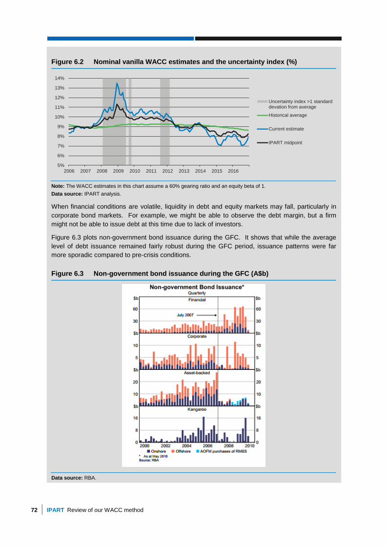
72 IPART Review of our WACC method
Figure 6.2 Nominal vanilla WACC estimates and the uncertainty index (%)
Note: The WACC estimates in this chart assume a 60% gearing ratio and an equity beta of 1.
Data source: IPART analysis.
When financial conditions are volatile, liquidity in debt and equity markets may fall, particularly in
corporate bond markets. For example, we might be able to observe the debt margin, but a firm
might not be able to issue debt at this time due to lack of investors.
Figure 6.3 plots non-government bond issuance during the GFC. It shows that while the average
level of debt issuance remained fairly robust during the GFC period, issuance patterns were far
more sporadic compared to pre-crisis conditions.
Figure 6.3 Non-government bond issuance during the GFC (A$b)
Data source: RBA.
5%
6%
7%
8%
9%
10%
11%
12%
13%
14%
2006 2007 2008 2009 2010 2011 2012 2013 2014 2015 2016
Uncertainty index >1 standarddevation from average
Historical average
Current estimate
IPART midpoint
Review of our WACC method IPART 73
This suggests:
the current estimate of the WACC may not always reflect debt raising costs incurred by firms
during periods of financial stress, and
firms avoid issuing debt and equity when these costs are at their highest, which would tend
to reduce their average cost of capital.
6.5 Re-estimate the gearing ratio at each price review
Our current approach is to review the gearing ratio each time we estimate the WACC for a
business, considering updated market data and decisions made by other regulators. In practice, the gearing ratio should be stable over time, particularly as most firms we regulate
operate a stable base of historic assets. On the other hand, the efficient gearing ratio for a
benchmark firm could change over time, for example, if there are changes in investor preferences, tax reforms or other policy changes.
In our Draft Report, we proposed to continue to re-estimate gearing at each price review.148
6.5.1 Stakeholders expressed a preference to review gearing outside of price
reviews
In response to our Draft Report, WaterNSW considered that “…an enhancement to the
regulatory process would be to conduct a review of the appropriate equity beta, gearing and
the selection of proxy firms outside of price reviews. This will provide IPART-regulated utilities with more certainty on these parameters ahead of price-review submissions, and
enhance the predictability and transparency of the IPART regulatory process”.149
SDP referred to its response to our Issues Paper, which was that it supported maintaining our current approach, but considers we should:
• use the capital structure of the benchmark firm
• have regard to other regulatory decisions, and
• only change our determination of the benchmark gearing if there is sufficient evidence to do
so.150
While Sydney Water had expressed reservations in its response to our Issues Paper, it was
satisfied with our draft position. In particular, it originally submitted that “gearing should
only be reviewed if there are obvious structural changes within Australia that would bring about the need to assess gearing”.151 It noted that if gearing was reviewed at each price
review, because the review was largely based on proxy international firms, it may “import
structural changes and unnecessary instability that may not be representative of the Australian experience”.152 However, it contended that if gearing were to be reviewed
periodically, “it is critical that such reviews are conducted sufficiently prior to each firm’s
148 IPART, Review of our WACC Method: Draft Report, October 2017, p 69. 149 WaterNSW submission to IPART Draft Report, December 2017, p 15. 150 SDP submission to IPART Issues Paper, August 2017, p 6. 151 Sydney Water submission to IPART Issues Paper, August 2017, p 16 152 Ibid, p 17.
74 IPART Review of our WACC method
price review to enable timely utility modelling and sound business plans to be developed
and submitted”.153
However, in response to our Draft Report, Sydney Water concluded:
..IPART’s draft position elaborated that gearing will be reviewed along with the beta and any
adjustments to the gearing will be backed by sufficient evidence. Further, IPART have stated they
will undertake reviews early in price review processes, allowing incorporation into price
submissions. On this basis, we accept this change.154
Hunter Water maintained its view, in response to our Draft Report, that:
Gearing should be reviewed prior to a price review to allow for enhanced accuracy in price
submission planning and modelling. An alternative would be that IPART indicate ahead of a price
review the likelihood of hearing changes in the context of new market data, significant financial
events or regulatory policy developments.155
6.5.2 Our final decision is to continue to review gearing at each price review
Overall, we consider that a periodic review (every 3-5 years) of gearing is good practice and
that we should review the gearing of the benchmark entity at the same time that we review
the equity beta. Both of these reviews would rely on the same proxy firm analysis.
We consider that given the stakeholder administration and consultation involved, it would
be pragmatic to do it within a price review (which generally occurs every 4-5 years). It also
allows a broader scope of stakeholders, including customer representative groups, to engage in the process, which they may otherwise not have the resources to do.
However, taking into account stakeholders’ views, we will undertake this analysis earlier in
the review process, to give stakeholders more time to consider our proxy firm selection, gearing and beta analysis and respond before we proceed with our draft decisions, which
would be based on the results. In line with Final Decision 27, we will also improve the
transparency of our process by:
publishing our criteria for proxy selection, and our list of comparator companies that
meet our criteria at the start of the relevant review, and
giving stakeholders the opportunity to propose additional comparable industries that meet our criteria, but not individual stocks.
As for the equity beta, we would not automatically change the gearing we use in WACC
calculations in line with the results of a periodic review. Rather, we would adjust it only if
there were sufficient evidence.
Final Decision
32 Continue to re-estimate the gearing of the benchmark entity at each price review to inform
our assessment of whether the existing estimates remain appropriate.
153 Ibid, p 7. 154 Sydney Water submission to IPART Draft Report, December 2017, p 6. 155 Hunter Water submission to IPART Draft Report, December 2017, p 12.

Review of our WACC method IPART 75
7 Measuring inflation and gamma
Under our 2013 method for setting the WACC, we first measure the cost of debt and equity in nominal terms. Therefore, in line with our policy of setting and applying a real post-tax
WACC, we need to adjust these nominal measurements by inflation to derive a real WACC.
Since December 2014, we have applied a single, forward-looking inflation forecast to both the current and historic costs. This forecast is the expected rate of inflation over the next 10
years, which we calculate as the geometric average of:
a current 1-year forecast based on quarterly data from the RBA’s Statement of Monetary Policy (SMP), and
the middle of the RBA’s target band for inflation (2.5%) for Years 2 to 10.
In this review, we have considered: what period over which we forecast inflation; whether we continue to estimate inflation using a geometric average method or use a breakeven
inflation method; and whether we should change our approach for calculating the geometric
average.
Another aspect of the impact of taxation on the WACC is the imputation credit factor,
gamma. We currently assume that gamma has a value of 0.25, and have considered whether
this remains appropriate.
The sections below provide an overview of our final decisions on inflation and gamma, and
then discuss them in more detail.
7.1 Overview of final decisions on inflation and gamma
We will continue to set a real post-tax WACC by adjusting our nominal cost estimates for
inflation. However, we have decided to make some modifications to our current approach
for this adjustment.
We will adjust both current and historic cost inputs by the expected rate of inflation over the
regulatory period instead of the next 10 years. We consider this will reduce the risk under
our current approach that, at different points in the economic cycle, we over- or under-
estimate inflation.
We will continue to use a geometric average method to calculate this rate of inflation
because, despite the in-principle benefits of using the break-even inflation method, as our analysis indicates that currently there is not a convincing case for change. However, we will
make two small modifications to the way we apply the method:
We will calculate expected inflation as the geometric average of the change in the
level of prices (rather than the inflation rate).
76 IPART Review of our WACC method
We will define the 1-year ahead RBA forecast as the inflation forecast in the RBA’s
most recently issued SMP that is closest to 12 months ahead of the start of the
regulatory period.
We have also decided to continue to use 0.25 as the value of gamma.
All of these final decisions are consistent with our draft decisions.
7.2 Setting a real post-tax WACC
As Chapter 2 discussed, in this review we are not considering broader policy issues related to how we apply the WACC in this review. We will continue to apply a real post-tax
WACC.
The post-tax framework avoids overcompensating firms who, in practice, tend to pay less than the statutory rate of tax. In many cases, the post-tax framework provides a more
accurate estimate of the revenue that regulated businesses require to meet their tax
obligations. This is consistent with the approach taken by many other Australian regulators, including the ACCC and AER (see Appendix A). We intend to review the way that we
apply the post-tax framework in the building block model in 2018.
By applying a real WACC to a RAB that we index for inflation, we ensure that inflation is accounted for only once. Indexing the RAB for inflation affects the price path and hence, the
business’ cash flow, even though it is net present value (NPV) neutral over the life of the
assets. That is because the decision to capitalise inflation alters the RAB and cash flow profile over time. Our financeability test allows us to examine whether the cash flows allow
the business to remain financially viable.
7.3 Adjust for expected inflation over the regulatory period
We currently deflate our nominal WACC inputs by applying a single, forward-looking rate
that is the expected rate of inflation over the next 10 years, regardless of the length of the
regulatory period. In our Issues Paper, we expressed a preliminary view to maintain our existing approach of using a 10-year forward-looking inflation rate for this adjustment.
7.3.1 Stakeholders suggested alternative approaches
Stakeholders expressed a range of views on this question. For example, Sydney Water did
not agree with our preliminary view, and stated that we should “use a best estimate of
expected inflation over the regulatory period instead of using long-term inflation expectations”.156 It also noted our current approach, which is an estimate of long-term
inflation expectations, might be “problematic when long-term inflation expectations differ
substantially from forecast inflation over the regulatory period”.157
156 Sydney Water submission to IPART Issues Paper, August 2017, p 7. 157 Ibid.

Review of our WACC method IPART 77
In contrast, NSW Treasury proposed that we calculate inflation on the same basis that the
risk-free rate is calculated.158 For example, if we set the WACC as the midpoint of a current
estimate and a historic average over the past 10 years, we should deflate the WACC by a
midpoint of a current and a historic estimate of inflation. In particular, deflating the historic estimate of the WACC by a historic estimate of inflation, would reflect the real cost of
finance at the time that debt, or equity, was issued.
7.3.2 Our draft decision was to maintain our existing approach
We agreed with Sydney Water’s response to our Issues Paper, including its concern about
our current approach. A 10-year geometric average, with a 2.5% inflation rate for nine out of the 10 years, would produce an inflation estimate that is very close to 2.5%. Therefore, at
different points in the economic cycle, there is a risk that our current approach would over-
or under-estimate actual inflation.
We did not agree with Treasury’s view, preferring a forward-looking inflation forecast over
the regulatory period as the appropriate measure to deflate the nominal WACC. This is
because the real WACC should reflect an efficient firm’s expected real cost of capital over a regulatory period. Even though the nominal cost of capital might reflect a mix of current
and historic debt and equity costs, it is the forward-looking inflation over the regulatory
period that matters. It would determine how that nominal cost of capital is converted to real terms. We noted that this could mean using a slightly different inflation rate in two
concurrent reviews, if we decide to set a different regulatory period for the businesses
concerned.
7.3.3 Stakeholders supported our draft decision
Stakeholders generally supported our draft decision.159 However, WaterNSW reiterated its support for using breakeven inflation (discussed below).160
Hunter Water supported our draft decision to adjust nominal WACC inputs by expected
inflation over the regulatory period.161
Final Decision
33 In converting our nominal WACC inputs into real terms, adjust them by the expected rate
of inflation over the regulatory period.
7.4 Use a geometric average method to calculate expected inflation
We currently calculate the expected inflation rate as the geometric average of the midpoint
of the RBA’s 1-year ahead inflation forecast and the midpoint of the RBA’s target inflation band. However, prior to 2009, we used the break-even inflation method (BEI method).
158 NSW Treasury submission to IPART Issues Paper, August 2017, p 5. 159 Sydney Water submission to IPART Draft Report, December 2017, p 6; WaterNSW submission to IPART
Draft Report, December 2017, p 15; Hunter Water submission to IPART Draft Report, December 2017, p 12, SDP submission to IPART Draft Report, December 2017, p 14.
160 WaterNSW submission to IPART Draft Report, December 2017, p 15. 161 Hunter Water submission to IPART Draft Report, December 2017, p 12.
78 IPART Review of our WACC method
The BEI method estimates inflation as the difference between the yield on an inflation linked
bond and a nominal bond of equivalent maturity (implied by the Fisher equation below), to
calculate expected inflation as the rate of inflation that would make an investor indifferent
between the two bonds:
(1 + 𝑖) ≡ (1 + 𝑟) × (1 + 𝜋𝑒) (7)
where:
i is the yield on the nominal bond
r is the yield on the inflation linked bond, and
𝜋𝑒 is the expected inflation rate.
Rearranging, the inflation rate under the BEI method is:
𝜋𝑒 = (1+𝑖
1+𝑟) − 1 (8)
In May 2009, we moved away from the BEI method, in part, due to concerns about the breadth of liquidity in the inflation-linked bond market.
The AER currently estimates inflation using a geometric average approach, forecasting
inflation as the geometric average of:
1-year and 2-year forecasts based on quarterly data from the RBA’s SMP, and
the middle of the RBA’s target (2.5%) for Years 3 to 10.
The AER recently reviewed its approach to inflation. In its final position paper, the AER
decided to estimate inflation using a geometric average method over other methods
including the BEI method because, in its view, it is ‘the simplest to apply, most transparent
and easily replicable’. 162
7.4.1 Some stakeholders supported moving back to the BEI method
In response to our Issues Paper, Sydney Water and SDP expressed some support for continuing to use a geometric average method.163 However, WaterNSW and Hunter Water
encouraged us to consider the BEI method.164 NSW Treasury strongly supported moving to
the BEI method. NSW Treasury preferred the BEI method because, in its view:
this method reflects the current market expectation of future inflation which feed
directly into the price of debt at the time of the measurement
RBA forecasts of inflation are only updated quarterly, and
other regulators, including OFGEM and ORR in the UK, use BEI method.165
162 AER, Regulatory treatment of inflation, Final position, December 2017, p 47. 163 Sydney Water submission to IPART Issues Paper, August 2017, p 18 and SDP submission to IPART Issues
Paper, August 2017, pp 42-43. 164 WaterNSW submission to IPART Issues Paper, August 2017, p 13 and Hunter Water submission to IPART
Issues Paper, August 2017, p 10. 165 NSW Treasury submission to IPART Issues Paper, August 2017, p 6.
Review of our WACC method IPART 79
NSW Treasury also provided evidence that previous concerns with BEI method are no
longer as acute:
The depth and liquidity of inflation-linked bond markets have improved significantly
in recent years, with investor demand, bond issuance and turnover data increasing significantly in recent years. In addition, the Australian Office of Financial
Management (AOFM) – which is responsible for issuing inflation-linked bonds – has
committed to maintaining an inflation-linked bond market.
Inflation and liquidity premia are likely to have fallen in line with the increase in the
size of the inflation-linked bond market.
7.4.2 Our draft decision was to maintain our existing approach and reconsider
moving to BEI method at next WACC review
We analysed the BEI method and the geometric average method to consider the points it
raised. In particular, we compared two methods using four criteria:
economic theory
reliability of market data
accuracy of historic forecasts, and
simplicity, transparency and replicability.
We found that, overall, that there was not a sufficient case to change from a geometric
average method to the BEI method. (Appendix E provides more detail on this analysis.)
Therefore, our draft decision was to continue to calculate the average expected inflation rate
using our geometric average approach, but reconsider whether we should move to a break-
even inflation method at the next review of our WACC method.166
7.4.3 Our final decision is in line with our draft decision
Stakeholders generally supported our draft decision.167 However, WaterNSW reiterated its
support for using the BEI method.168
We recognise the in-principle benefits of using the BEI method to calculate inflation.
However, on-balance, we have decided to maintain our draft decision to use a geometric
average approach as we consider that currently, there is not a sufficient case for change:
1. While our analysis suggests that liquidity in the inflation-linked bond market not
currently an acute concern, we remain concerned that the market may not remain
sufficiently liquid throughout the business cycle. Therefore, the accuracy of the BEI method may vary at different points in the economic cycle.
2. In part, due to data limitations, the BEI method is a slightly more complex, and less
replicable, method compared to a geometric average.
166 IPART, Review of our WACC Method: Draft Report, October 2017, p 81. 167 Sydney Water submission to IPART Draft Report, December 2017, p 6; WaterNSW submission to IPART
Draft Report, December 2017, p 15; Hunter Water submission to IPART Draft Report, December 2017, p 12, SDP submission to IPAER Draft Report, December 2017, p 14; PIAC submission to our Draft Report, December 2017, p 3.
168 Hunter Water submission to IPART Draft Report, December 2017, p 12.
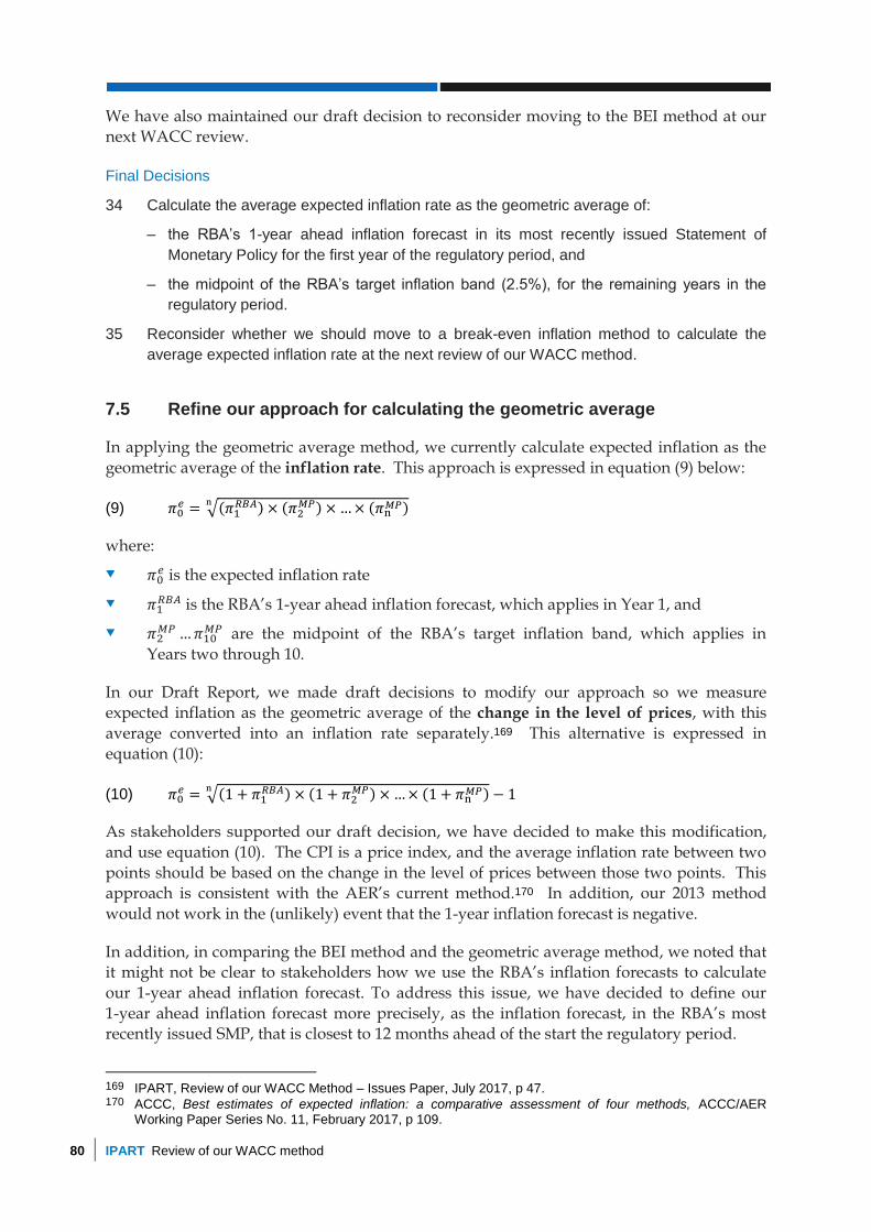
80 IPART Review of our WACC method
We have also maintained our draft decision to reconsider moving to the BEI method at our
next WACC review.
Final Decisions
34 Calculate the average expected inflation rate as the geometric average of:
– the RBA’s 1-year ahead inflation forecast in its most recently issued Statement of
Monetary Policy for the first year of the regulatory period, and
– the midpoint of the RBA’s target inflation band (2.5%), for the remaining years in the
regulatory period.
35 Reconsider whether we should move to a break-even inflation method to calculate the
average expected inflation rate at the next review of our WACC method.
7.5 Refine our approach for calculating the geometric average
In applying the geometric average method, we currently calculate expected inflation as the
geometric average of the inflation rate. This approach is expressed in equation (9) below:
𝜋0𝑒 = √(𝜋1
𝑅𝐵𝐴) × (𝜋2𝑀𝑃) × … × (𝜋n
𝑀𝑃)n (9)
where:
𝜋0𝑒 is the expected inflation rate
𝜋1𝑅𝐵𝐴 is the RBA’s 1-year ahead inflation forecast, which applies in Year 1, and
𝜋2𝑀𝑃 … 𝜋10
𝑀𝑃 are the midpoint of the RBA’s target inflation band, which applies in
Years two through 10.
In our Draft Report, we made draft decisions to modify our approach so we measure expected inflation as the geometric average of the change in the level of prices, with this
average converted into an inflation rate separately.169 This alternative is expressed in
equation (10):
𝜋0𝑒 = √(1 + 𝜋1
𝑅𝐵𝐴) × (1 + 𝜋2𝑀𝑃) × … × (1 + 𝜋n
𝑀𝑃)n− 1 (10)
As stakeholders supported our draft decision, we have decided to make this modification,
and use equation (10). The CPI is a price index, and the average inflation rate between two
points should be based on the change in the level of prices between those two points. This approach is consistent with the AER’s current method.170 In addition, our 2013 method
would not work in the (unlikely) event that the 1-year inflation forecast is negative.
In addition, in comparing the BEI method and the geometric average method, we noted that it might not be clear to stakeholders how we use the RBA’s inflation forecasts to calculate
our 1-year ahead inflation forecast. To address this issue, we have decided to define our
1-year ahead inflation forecast more precisely, as the inflation forecast, in the RBA’s most recently issued SMP, that is closest to 12 months ahead of the start the regulatory period.
169 IPART, Review of our WACC Method – Issues Paper, July 2017, p 47. 170 ACCC, Best estimates of expected inflation: a comparative assessment of four methods, ACCC/AER
Working Paper Series No. 11, February 2017, p 109.
Review of our WACC method IPART 81
Final Decisions
36 Calculate expected inflation as the geometric average of the change in the level of prices.
37 Define the 1-year ahead RBA forecast we use to estimate inflation, as the inflation
forecast:
– in the RBA’s most recently issued Statement of Monetary Policy, and
– that is closest to 12 months ahead of the start of the regulatory period.
7.6 Use 0.25 as the value of gamma
Under the Australian imputation tax system, shareholders may receive dividends with
imputation tax credits, which offset tax liabilities. Therefore, investors would accept a lower
rate of return for an investment with imputation credits attached than if there were no imputation tax credits attached.
The imputation credit factor, gamma, is most relevant for converting a post-tax WACC to a
pre-tax WACC. As we have adopted a post-tax WACC framework, we do not directly use gamma in our calculations. However, as noted in Chapter 5, gamma does have an influence
over the current MRP estimates we use.
7.6.1 How we derived our point estimate of gamma used in our 2013 method
We have used a 0.25 value of gamma since our December 2011 pricing decision for SDP.
That decision took account of a dividend drop-off study by then SFG Consulting (SFG)171 that was done for the Australian Competition Tribunal. This value was reconfirmed by a
follow-up report by SFG that was done for Jemena Gas Networks in 2015.
SFG based its estimate primarily on implied market valuation methods, such as dividend drop-off studies. Such studies compare the value of equities in specific firms just before and
just after a dividend is paid. While these estimates tend to be ‘noisy’, the underlying signal
contains information about the value investors place on those dividends, taking full account of their tax position and ability to use imputation credits.
SFG also undertook another study, which took into account valuation information obtained
from analysis of equity ownership and of Australian Taxation Office (ATO) taxation statistics. The equity ownership method uses data from the Australian Bureau of Statistics
(ABS) to determine what proportion of Australian equity is held by domestic investors and
what proportion by foreign investors. The main assumption of the method is that domestic
investors take full advantage of imputation credits while foreign investors are unable to take
any advantage of them. While providing a point of reference, this assumption is imprecise,
and may tend to overestimate the use of imputation credits. Further, domestic ownership ratios fluctuate considerably over time, and are quite different for listed equities as
compared to all (listed and non-listed) equities. All of these factors tend to make the equity
ownership method imprecise.
171 SFG is now part of Frontier Economics.
82 IPART Review of our WACC method
The ATO taxation statistics approach uses aggregate data on the tax returns of payers of
Australian tax. From this data it is possible to understand the extent to which taxpayers
actually claim imputation credits. While this method also has its limitations, it tends to
produce gamma estimates that are lower than those from the equity ownership method, because it does not make such imprecise assumptions about the behaviour of investors.
7.6.2 Most stakeholders supported gamma of 0.25
Most stakeholders supported gamma of 0.25. In its submission to our Issues Paper, SDP
included a report from Frontier Economics that maintains that the best dividend drop-off
(market value) estimate of gamma currently available is 0.25.172 Frontier Economics contends that there are two possible interpretations of gamma: a market value concept,
under which gamma represents the price that an investor would be willing to pay for an
imputation credit; and, a redemption or utilisation concept, which represents the rate at which imputation tax credits are redeemed by taxpayers to reduce their personal tax
liabilities. Under IPART’s framework, gamma is the amount by which the total allowed
return on equity is reduced to reflect the imputation credits that investors will receive. As such, it must reflect the market value of credits relative to dividends and capital gains. This
suggests that the market value interpretation is appropriate.173
However, PIAC expressed concerns that this value is significantly lower than the gamma value used by other regulators. It noted that the “…Australian Competition Tribunal since
found in favour of the AER’s calculation of a gamma of 0.4 in its decision regarding SA
Power Networks, as did the Full Federal Court with respect to the AER’s decision regarding the NSW and ACT DNSPs [Distribution network service providers]”.174
Stakeholders made no further comments about gamma in submissions to our Draft Report.
7.6.3 We consider there is not sufficient evidence to adopt a different value of
gamma at this time
Unfortunately, because it is not possible to directly observe the after-tax returns that
investors make, gamma is extremely difficult to establish empirically. We acknowledge that
other regulators adopt different values for gamma (see Appendix A) and at times the selection of gamma has been controversial.
In recent years, some regulators have moved towards a higher value of gamma than 0.25.175
In 2016, the SA Power Networks (SAPN) appealed the AER’s final determination that the valued attributed to gamma should be 0.4 to the Australian Competition Tribunal (ACT).
SAPN’s proposal was a value of 0.25.176 In its final decision, the ACT noted the difficulties
in estimating gamma accurately from market data. It stated:
172 Frontier Economics, Review of WACC method: response to IPART Issues Paper: A report prepared for
Sydney Desalination Plant, August 2017, p 52. 173 Ibid, p 45. 174 PIAC submission to IPART Issues Paper, August 2017, p 3. 175 See Appendix A – this includes the AER, ACCC and ERAWA which have adopted 0.4 and the QCA, which
adopted 0.47. 176 Australian Competition Tribunal, Final decision on application by SA Power Networks, 2016, paragraph 125.

Review of our WACC method IPART 83
Unfortunately, the available empirical evidence is inadequate to enable confident discrimination
between these alternative perspectives. There are a range of studies, reviewed in the AER’s Final
Decision, using market prices which attempt to estimate the extent to which imputation credits are
capitalised into stock prices and thus their market valuation. There are a range of results, and
experts are divided on the merits of the various approaches and techniques
Ultimately, the ACT found in favour of the AER’s value of gamma, its reasoning being:
…the AER did not err, nor was unreasonable, in giving most weight to the “utilisation” approach. It
considered the range of alternative approaches, recognised the diversity of views of experts on
their merits (both theoretical and empirical), and made a judgement call. In doing so, it
demonstrated responsiveness to the empirical evidence in lowering its estimate of gamma from
0.5 as proposed in its ROR Guidelines to a value of 0.4.177
However, while the ACT found that the AER’s decision-making process for arriving at its
value of gamma was not unreasonable in the circumstances, this does not necessarily infer
that the ACT endorsed the AER’s decision.
We agree with Frontier Economics that the value of gamma should be interpreted as the market value of dividends and capital gains that investors would be willing to forgo in
exchange for imputation credits.178 Further, we maintain our view that dividend drop-off
studies are currently the best method to estimate the market value of gamma. Its advantage is that it measures the observed value of dividends and imputation credits by examining
share price changes on ex-dividend days.
Since the 2011 SFG study that we relied upon in our 2013 method, Frontier updated its analysis in 2013179 and again in 2017180. The latter study employed a large sample and
improved econometric techniques to estimate the value of both cash dividends and
distributed imputation credits using dividend drop-off analysis. Both of these studies reconfirmed that the best estimate of the market value of gamma was 0.25.
7.6.4 Our final decision is to continue to use 0.25
Based on our analysis and stakeholder feedback, we consider that there is not sufficient
evidence to suggest a more accurate method of determining gamma. Hence, to maintain
stability and certainty for stakeholders, we propose to continue using our current value of gamma of 0.25.
We will continue to monitor developments in this area, and will consider whether we
should change our approach to gamma at our next WACC review.
Final Decision
38 Continue to use 0.25 as the value for gamma.
177 Ibid, pp 158-159. 178 Frontier Economics, p 51. 179 Frontier Economics, Updated dividend drop-off estimate of theta: Report for the Energy Networks
Association, June 2013. 180 Forthcoming paper by Damien Cannavan and Stephen Gray, Dividend drop-off estimates of the value of
dividend imputation tax credits, 2017.

84 IPART Review of our WACC method

Review of our WACC method IPART 85
Appendices

86 IPART Review of our WACC method
A Comparison of other regulators’ approaches to WACC
Table A.1 Comparison of IPART, AER, ACCC and ESC Victoria’s recent approaches181
IPARTa AERb ACCCc ESCd
Date updated Feb 2018 Dec 2013 Apr 2017 (rail) Oct 2016 (water)
Application
Type of WACC Real post-tax Nominal vanilla post-tax Real pre-tax WACC Real post-tax
Definition of benchmark entity
"A benchmark firm operating in a competitive market and facing similar risks to the regulated business".
"A pure play, regulated energy network business operating within Australia".
- -
Point estimate or range
Default is midpoint of estimate range for each parameter derived from long and current market data.
Point estimate Point estimate Point estimate based on weighting of 60:40 return on debt to return on equity. However, while a benchmark cost of debt applies, return on equity is determined over a range of values linked to tangible outcomes to customers according to ‘PREMO’ framework.
Adjustment mechanism
Uncertainty index constructed from four proxies for economic uncertainty in Australia. If UI outside one standard deviation from mean, we will consider
There are multiple reasonableness checks and adjustments before finalising cost of debt and equity components.
- WACCs are adjusted based on level of ambition proposed by the business.
181 This comparison table is compiled from a combination of WACC statements of approach (where published) and recent regulatory decisions. It may not reflect the
methodology that applies to all industries. We have noted the approach is specific to one industry.
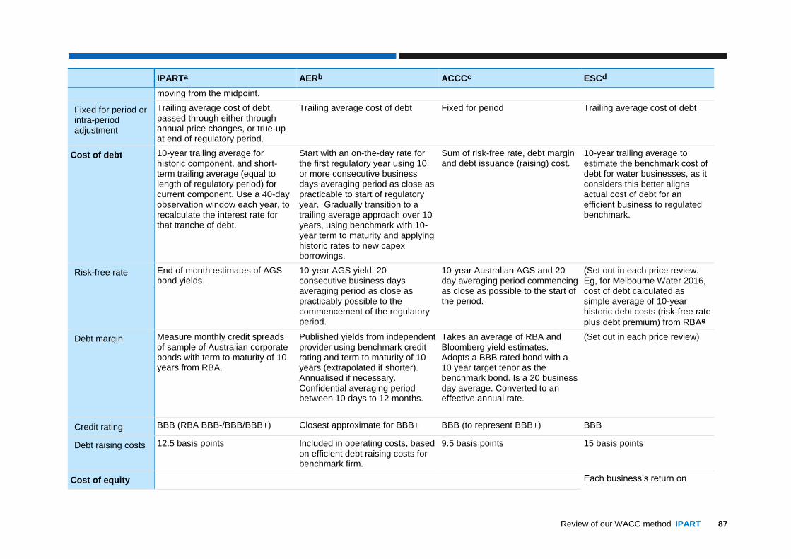
Review of our WACC method IPART 87
IPARTa AERb ACCCc ESCd
moving from the midpoint.
Fixed for period or intra-period adjustment
Trailing average cost of debt, passed through either through annual price changes, or true-up at end of regulatory period.
Trailing average cost of debt Fixed for period Trailing average cost of debt
Cost of debt 10-year trailing average for historic component, and short-term trailing average (equal to length of regulatory period) for current component. Use a 40-day observation window each year, to recalculate the interest rate for that tranche of debt.
Start with an on-the-day rate for the first regulatory year using 10 or more consecutive business days averaging period as close as practicable to start of regulatory year. Gradually transition to a trailing average approach over 10 years, using benchmark with 10-year term to maturity and applying historic rates to new capex borrowings.
Sum of risk-free rate, debt margin and debt issuance (raising) cost.
10-year trailing average to estimate the benchmark cost of debt for water businesses, as it considers this better aligns actual cost of debt for an efficient business to regulated benchmark.
Risk-free rate End of month estimates of AGS bond yields.
10-year AGS yield, 20 consecutive business days averaging period as close as practicably possible to the commencement of the regulatory period.
10-year Australian AGS and 20 day averaging period commencing as close as possible to the start of the period.
(Set out in each price review. Eg, for Melbourne Water 2016, cost of debt calculated as simple average of 10-year historic debt costs (risk-free rate
plus debt premium) from RBAe
Debt margin Measure monthly credit spreads of sample of Australian corporate bonds with term to maturity of 10 years from RBA.
Published yields from independent provider using benchmark credit rating and term to maturity of 10 years (extrapolated if shorter). Annualised if necessary. Confidential averaging period between 10 days to 12 months.
Takes an average of RBA and Bloomberg yield estimates. Adopts a BBB rated bond with a 10 year target tenor as the benchmark bond. Is a 20 business day average. Converted to an effective annual rate.
(Set out in each price review)
Credit rating BBB (RBA BBB-/BBB/BBB+) Closest approximate for BBB+ BBB (to represent BBB+) BBB
Debt raising costs 12.5 basis points Included in operating costs, based on efficient debt raising costs for benchmark firm.
9.5 basis points 15 basis points
Cost of equity Each business’s return on
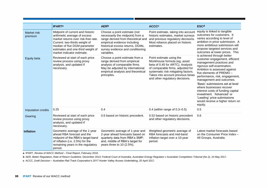
88 IPART Review of our WACC method
IPARTa AERb ACCCc ESCd
Market risk premium
Midpoint of current and historic arithmetic average of excess market returns over risk-free rate. Current: two-thirds weight of median of five DGM parameter estimates and one-third weight of market indicator estimate.
Choose a point estimate (not necessarily the midpoint) from a range derived from theoretical and empirical evidence including historical excess returns, DGMs, survey evidence and conditioning variables.
Point estimate, taking into account historic estimates, market surveys and previous regulatory decisions. Most reliance placed on historic estimates.
equity is linked to tangible outcomes for customers. It varies according to level of ambition in price submission. A more ambitious submission will propose targeted services and outcomes at lower prices. This is achieved through better customer engagement, efficient management practices and rigorous self-examination. Ambition is assessed against five elements of PREMO – performance, risk, engagement, management and outcomes.
‘Basic’ submissions set at level where businesses recover interest costs of funding capital investment. ‘Advanced’ or ‘Leading’ price submissions would receive a higher return on equity.
Equity beta Reviewed at start of each price review process using proxy analysis, and updated if necessary.
Choose a point estimate from a range derived from empirical analysis of comparable firms. May be adjusted by international empirical analysis and theoretical principles.
Point estimate using the Monkhouse formula (eg, asset beta of 0.45 for ARTC). Analysis of comparable firms, adjusted for systematic risk mitigating factors. Takes into account previous betas and other regulatory decisions.
Imputation credits 0.25 0.4 0.4 (within range of 0.3–0.5) 0.5
Gearing Reviewed at start of each price review process using proxy analysis, and updated if necessary.
0.6 based on historic precedent. 0.52 based on historic precedent and other regulatory decisions.
0.6
Inflation Geometric average of the 1-year ahead RBA forecast and the midpoint of the RBA’s target band of inflation (i.e. 2.5%) for the remaining years in the regulatory period.
Geometric average of 1-year and 2-year ahead forecasts based on quarterly data from RBA’s SMP; and, middle of RBA’s target for years three to 10 (2.5%).
Weighted geometric average of RBA forecasts and mid-band inflation target over a 10-year period.
Latest market forecasts based on the Consumer Price Index – All Groups, Australia.
a IPART, Review of WACC Method – Final Report, February 2018.
b AER, Better Regulation, Rate of Return Guideline, December 2013; Federal Court of Australia, Australian Energy Regulator v Australian Competition Tribunal (No 2), 24 May 2017.
c ACCC, Draft Decision – Australian Rail Track Corporation’s 2017 Hunter Valley Access Undertaking, 20 April 2017.

Review of our WACC method IPART 89
d Essential Services Commission, Water Pricing Framework and Approach, Implementing PREMO from 2018, October 2016; Essential Services Commission, Melbourne Water 2016 Price Review
– Guidance Paper, April 2015.
Table A.2 Comparison of QCA, ERAWA, ESCOSA and NZCC’s recent approaches
QCAa ERAWAb ESCOSAc NZCCd
Date updated Aug 2014 (equity)
Apr 2015 (debt)
Oct 2017 (rail) Mar 2015 (water) Dec 2016
Application
Type of WACC Nominal vanilla post-tax Real pre-tax Real post-tax Vanilla post-tax
Definition of benchmark entity
Pure play, regulated, standalone.
- “The regulatory return should be based on the expected behaviour of a benchmark efficient entity”
-
Point estimate or range
Point estimate Point estimate Point estimate Percentile along a distribution, which is industry-specific.
Adjustment mechanism
- - - Standard errors for asset beta, debt premium and MRP combined to determine WACC standard error. Based on industry, either midpoint or point along the distribution selected.
Additional reasonableness checks apply to ensure WACC realistic in light of financial market conditions.
Fixed or intra-period adjustment
Fixed over period - rejected trailing average debt in 2015
Fixed over period Trailing average cost of debt Fixed over period - rejected trailing average debt in 2016
Cost of debt ‘On the day' approach using benchmark cost of debt estimated just prior to start of regulatory cycle.
‘On the day’ observed rate for the next 10 years.
Weighted 10-year average approach – cost of debt updated each year of regulatory period.
Averages risk-free rate and debt premium over three calendar months just prior to start of regulatory period.
Risk-free rate Based on Australian Government bond yields over 20-day averaging period and
Observed yield of 10-year Australian Government Securities (AGS) from Treasury
Observed yields from 10-year Commonwealth Government Bonds averaged over 20
Government bond rates as using yield to maturity as an approximation of spot rates.
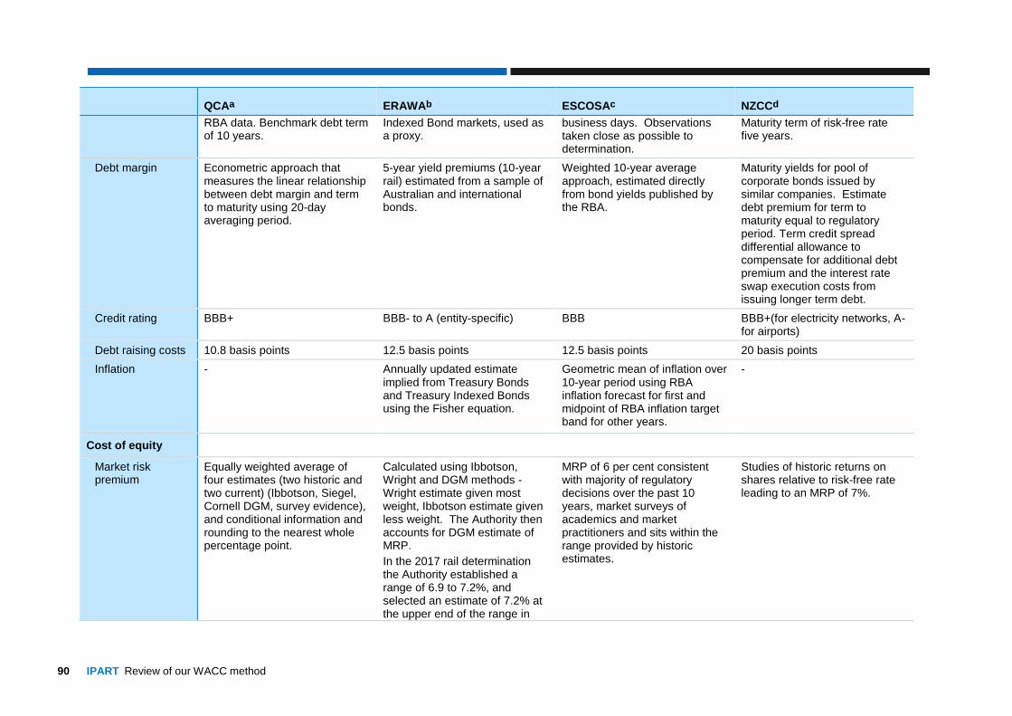
90 IPART Review of our WACC method
QCAa ERAWAb ESCOSAc NZCCd
RBA data. Benchmark debt term of 10 years.
Indexed Bond markets, used as a proxy.
business days. Observations taken close as possible to determination.
Maturity term of risk-free rate five years.
Debt margin Econometric approach that measures the linear relationship between debt margin and term to maturity using 20-day averaging period.
5-year yield premiums (10-year rail) estimated from a sample of Australian and international bonds.
Weighted 10-year average approach, estimated directly from bond yields published by the RBA.
Maturity yields for pool of corporate bonds issued by similar companies. Estimate debt premium for term to maturity equal to regulatory period. Term credit spread differential allowance to compensate for additional debt premium and the interest rate swap execution costs from issuing longer term debt.
Credit rating BBB+ BBB- to A (entity-specific) BBB BBB+(for electricity networks, A- for airports)
Debt raising costs 10.8 basis points 12.5 basis points 12.5 basis points 20 basis points
Inflation - Annually updated estimate implied from Treasury Bonds and Treasury Indexed Bonds using the Fisher equation.
Geometric mean of inflation over 10-year period using RBA inflation forecast for first and midpoint of RBA inflation target band for other years.
-
Cost of equity
Market risk premium
Equally weighted average of four estimates (two historic and two current) (Ibbotson, Siegel, Cornell DGM, survey evidence), and conditional information and rounding to the nearest whole percentage point.
Calculated using Ibbotson, Wright and DGM methods - Wright estimate given most weight, Ibbotson estimate given less weight. The Authority then accounts for DGM estimate of MRP.
In the 2017 rail determination the Authority established a range of 6.9 to 7.2%, and selected an estimate of 7.2% at the upper end of the range in
MRP of 6 per cent consistent with majority of regulatory decisions over the past 10 years, market surveys of academics and market practitioners and sits within the range provided by historic estimates.
Studies of historic returns on shares relative to risk-free rate leading to an MRP of 7%.
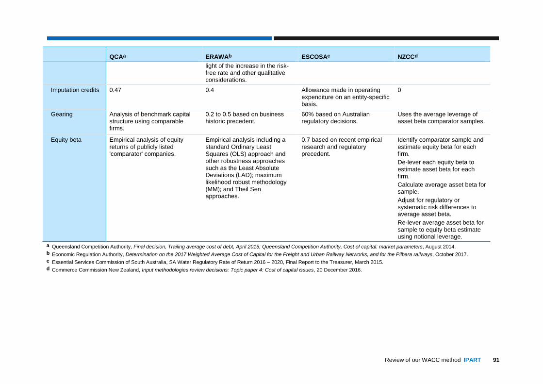
Review of our WACC method IPART 91
QCAa ERAWAb ESCOSAc NZCCd
light of the increase in the risk-free rate and other qualitative considerations.
Imputation credits 0.47 0.4 Allowance made in operating expenditure on an entity-specific basis.
0
Gearing Analysis of benchmark capital structure using comparable firms.
0.2 to 0.5 based on business historic precedent.
60% based on Australian regulatory decisions.
Uses the average leverage of asset beta comparator samples.
Equity beta Empirical analysis of equity returns of publicly listed 'comparator' companies.
Empirical analysis including a standard Ordinary Least Squares (OLS) approach and other robustness approaches such as the Least Absolute Deviations (LAD); maximum likelihood robust methodology (MM); and Theil Sen approaches.
0.7 based on recent empirical research and regulatory precedent.
Identify comparator sample and estimate equity beta for each firm.
De-lever each equity beta to estimate asset beta for each firm.
Calculate average asset beta for sample.
Adjust for regulatory or systematic risk differences to average asset beta.
Re-lever average asset beta for sample to equity beta estimate using notional leverage.
a Queensland Competition Authority, Final decision, Trailing average cost of debt, April 2015; Queensland Competition Authority, Cost of capital: market parameters, August 2014.
b Economic Regulation Authority, Determination on the 2017 Weighted Average Cost of Capital for the Freight and Urban Railway Networks, and for the Pilbara railways, October 2017.
c Essential Services Commission of South Australia, SA Water Regulatory Rate of Return 2016 – 2020, Final Report to the Treasurer, March 2015.
d Commerce Commission New Zealand, Input methodologies review decisions: Topic paper 4: Cost of capital issues, 20 December 2016.
92 IPART Review of our WACC method
B How we will update the cost of debt measurements
Under our 2013 WACC method, we set the cost of debt as a midpoint of a current and a historic estimate. We set the cost of debt for the duration of the regulatory period and do
not update it until the next period.
As part of the consultation on our review of the WACC method, stakeholders proposed that we change our approach to estimating the cost of debt to update the cost of debt every year
of the regulatory period.
We have decided to update the cost of debt annually, and maintain a midpoint of current and historic costs.
For the historic estimate, we will estimate the cost of debt as a 10-year trailing average
by splitting the historic debt into 10 equal parts, or ‘tranches’, with staggered dates of commencement and maturity.
For the current estimate, we will split the current debt into tranches equalling the
number of years in the regulatory period. The commencement and maturity dates for each tranche would be staggered so that one tranche would be refinanced the
beginning of each year, effectively forming a short-term trailing average.
We will also decide whether the updated cost of debt should feed through to prices on an
annual basis (annual update) or in the subsequent regulatory period (true-up). This
appendix provides the formulae for calculating the annual update and the true-up.
The notation we use in the formulae below is explained in Box B.1.
Box B.1 Nomenclature for the formulae below
y A year index where y=0 for the beginning of the first regulatory period of the new method.
T The tenor of debt.
n The number of years in the regulatory period.
R(y,T) The prevailing interest rate in year y for a bond of tenor T, measured over the 40-day
observation window.
Debt The average value of the firm’s debt over the regulatory period, estimated by applying the
benchmark gearing ratio we decided for the firm.
WACC The WACC we set at the beginning of the current regulatory period.
F The time value of money discount factor = 1 + WACC
TU the true-up in dollars on the first day of the next regulatory period

Review of our WACC method IPART 93
B.1 Formulae for annual update
Table B.1 provides the formulae for adjusting the cost of debt with an annual update for both the current and historic debt estimates.
At the beginning of the first regulatory period (y=0), the cost of debt is initially set as an
average over the past 10 years for the historic estimate and as a 40-day average for the current estimate, ie:
∑ 𝑅(−𝑘, 10)/109𝑘=0 for the historic estimate, and
R(0,10) for the current estimate.
The subsequent rows in Table B.1 outline how we will change the cost of debt in future years with updated interest rate data.
Table B.1 Adjustment formulae for the annual update
What When Add Remove
Historic cost of debt
Start of first period (y=0) Average of annual interest rates (40
working day observation window)
∑ 𝑅(−𝑘, 10)/10
9
𝑘=0
N/A
(No adjustment)
During first period R(y,10)/10 R(y-10,10)/10
Start of subsequent periods
R(y,10)/10 R(y-10,10)/10
During subsequent periods
R(y,10)/10 R(y-10,10)/10
Current cost of debt
Start of first period (y=0) Prevailing cost of debt (40 day observation
window)
R(0,10)
N/A
(No adjustment)
During first period R(y,10)/n R(0,10)/n
Start of subsequent periods
R(y,10)/n R(y-n,10)/n
During subsequent periods
R(y,10)/n R(y-n,10)/n
B.2 Formulae for true-up
If we decide to update the cost of debt in the subsequent regulatory period, we would need to account for the time value of money in order to make these changes NPV neutral. In
Section 4.7 we outline why we will use the WACC that we set at the beginning of each
regulatory period, as the discount factor.
Because there is no transition period for implementing a 10-year trailing average to estimate
the historic cost of debt, we will calculate the true-up (TU) using equation 1 at the end of
each period:

94 IPART Review of our WACC method
𝑇𝑈 = 𝐷𝑒𝑏𝑡
20∑ (𝑛 − 𝑦)(𝑅(𝑦, 10) − 𝑅(𝑦 − 10,10))𝐹
𝑛−𝑦
2𝑛−1𝑦=1 (11)
Equation 11 takes the change in the interest rate in each year of the regulatory period, for the
2nd year to the final year of an n year regulatory period, and then discounts these differences by the WACC to account for time value of money.
Because we will transition to the short-term trailing average over the first regulatory period,
the true-up for the current cost of debt will be different for this period, as shown in equation 12:
𝑇𝑈 = 𝐷𝑒𝑏𝑡
2×𝑛∑ (𝑛 − 𝑦)(𝑅(𝑦, 10) − 𝑅(0,10))𝐹
𝑛−𝑦
2𝑛−1𝑦=1 (12)
The true-up for the current cost of debt in subsequent periods is shown in equation 13:
𝑇𝑈 = 𝐷𝑒𝑏𝑡
2×𝑛∑ (𝑛 − 𝑦)(𝑅(𝑦, 10) − 𝑅(𝑦 − 𝑛, 10))𝐹
𝑛−𝑦
2𝑛−1𝑦=1 (13)

Review of our WACC method IPART 95
C Our analysis on the appropriate CAPM model
C.1 We consider the Black CAPM would produce similar results to SL-CAPM with adjustments for bias in the equity beta estimation
Both the SL-CAPM and Black CAPM predict the expected return of an asset is a function of its covariance with systematic (undiversifiable) risk. The main difference between these
models is the interpretation of the intercept term. The SL-CAPM uses the contemporaneous
risk-free rate of return, while the Black CAPM adopts the return of the minimum-variance
zero-beta portfolio of assets. The return of the zero-beta portfolio is greater than the
risk-free rate, but lower than the return of the market portfolio.182
In an abridged form, the expected return of an asset under the SL-CAPM (S) and Black CAPM (B) are:
(𝑆) 𝑟𝑖 = 𝑟𝑓 + 𝛽(𝑟𝑀 − 𝑟𝑓) (14)
(𝐵) 𝑟𝑖 = 𝑟𝑍 + 𝛽(𝑟𝑀 − 𝑟𝑍) (15)
where ri is the return on asset i, rf is the risk-free rate of return, rM is the return on the market
portfolio, and rZ is the return on the zero-beta portfolio. In essence, the SL-CAPM predicts a
lower intercept (as rf < rZ) and a higher slope (β) than the Black CAPM.
The observed relationship between the equity beta and subsequent return is much ‘flatter’
under the Black CAPM than predicted by the SL-CAPM.183 For stocks with estimated equity
betas below (above) one, realised returns tend to be higher (lower) than predicted under the Black CAPM. Figure C.1 demonstrates that observed results more closely reflect the
estimates of the Black CAPM than the SL CAPM, with a lower slope parameter and a higher
intercept.
182 Sharpe, W, Capital Asset Prices: A Theory of Market Equilibrium under Conditions of Risk, The Journal of
Finance, Vol 19, No. 3, September 1964, pp 425-442; Lintner, J, The Valuation of Risk Assets and the Selection of Risky Investments in Stock Portfolios and Capital Budgets, The Review of Economics and Statistics, Vol. 47, No. 1, February 1965, pp 13-37; Black, F, Capital Market Equilibrium with Restricted Borrowing, The Journal of Business, Vol. 45, No. 3, July 1972, pp 444-455.
183 Fama, E, and K French, The capital asset pricing model: Theory and evidence, Journal of Economic Perspectives, Vol. 18(3), 2004, p 32.

96 IPART Review of our WACC method
Figure C.1 Average annualised monthly return versus equity beta, 1928 to 2003
Note: Data points represent the annualised average value-weighted monthly returns of US equity portfolios decile-sorted on
prior-year beta. The furthest left observation therefore represents the average return on the lowest-decile beta stocks, with the
furthest right observation representing returns for the highest-decile beta stocks.
Data source: Fama, E, and K French, The capital asset pricing model: Theory and evidence, Journal of Economic
Perspectives, Vol 18(3), 2004, p 33.
At face value, the evidence suggests that the Black CAPM addresses the downward bias of
the SL-CAPM. This is especially relevant for regulated entities, as they typically exhibit
equity betas of less than one.
However, our current approach implements an adjustment to our estimated equity betas to
correct this potential bias. Empirical evidence suggests that equity betas obtained from
ordinary least squares (OLS) estimation are likely to be subject to a high degree of estimation bias due to sampling error. To correct for this bias, we implement the Vasicek adjustment.184
This adjusts OLS equity beta estimates towards the best prior equity beta estimate, with the
degree of adjustment based on estimated standard errors. In essence, the Vasicek adjustment gives a higher weight to more precisely estimated equity betas, and a lower
weight to estimated equity betas with higher standard errors.
Although the Vasicek adjustment is not explicitly designed to address the downward bias of the SL-CAPM, in practice, it can partly compensate for this bias. This is because very low or
very high beta estimates are relatively more likely to be to be affected by estimation error.185
For example, using a recent sample of proxy firms,186 we compared estimated OLS equity
betas to the change in equity beta due to the Vasicek adjustment. As Figure C.2 shows, the
Vasicek adjustment increases the estimates of low-beta firms, and decreases the estimates of
high-beta firms.
184 Vasicek, O, A Note on Using Cross-Sectional Information in Bayesian Estimation of Security Betas, The
Journal of Finance, Vol. 28, No. 5, December 1973, pp 1233-1239. 185 Gray, S and J Hall, SFG Consulting and Diamond, N and R Brooks, Monash University, The Vasicek
adjustment to beta estimates in the Capital Asset Pricing Model, June 2013, p 4. 186 Airport proxy firms as cited in: IPART, Maximum fees and charges for cruise ships Sydney Harbour – Final
Report, November 2016, p 99.

Review of our WACC method IPART 97
Cost of equity estimates under the Black CAPM may still be higher than under our adjusted
SL-CAPM due to the use of rZ as the intercept. However, in our view, the adjusted equity
beta estimates sufficiently account for the known downward bias of the SL-CAPM.
Figure C.2 OLS versus Vasicek-adjusted equity beta estimates, IPART airport proxy
firms
Note: Difference is defined as Vasicek beta minus OLS beta. Positive differences indicate the Vasicek adjustment increased
the OLS estimate, while negative differences indicate the adjustment lowered the OLS estimate. The adjusted R2 value is 0.7
Data source: Airport proxy firms as cited in: IPART, Maximum fees and charges for cruise ships Sydney Harbour – Final
Report, November 2016, p 99.
C.2 We will monitor results produced by the Fama-French Model over the next five years
The Fama-French three-factor model187 (FFM) follows empirical evidence that factors in
addition to systematic and firm risks affect stock returns. In addition to a systematic
(market) risk factor, the FFM also calculates a firm’s expected return as a function of pricing factors that proxy firm size and book-to-market effects. The expected return of an asset
under the FFM is:
𝑅𝑖 − 𝑅𝑓 = 𝛽𝑚𝑘𝑡(𝑅𝑀 − 𝑅𝑓) + 𝛽𝑠𝑖𝑧𝑒𝑆𝑀𝐵 + 𝛽𝑣𝑎𝑙𝑢𝑒𝐻𝑀𝐿 (16)
187 Fama, E and K French, Common Risk Factors in the Returns on Stocks and Bonds, Journal of Financial
Economics, Volume 33, No. 1, February1993, pp 3-56.
98 IPART Review of our WACC method
where ri is the return on asset i, rf is the risk-free rate of return, rM is the return on the market
portfolio, SMB and HML are factors capturing the excess return of small and high
book-to-market ratios (B/M-ratio) firms respectively, and β are factor sensitivities.
Both Australian188 and international189 evidence suggests that small firms earn higher excess returns on average than their larger counterparts, while high B/M-ratio firms earn higher
excess returns on average than low B/M-ratio firms. This is why the FFM results in greater
explanatory power in the cross-section of equity returns when compared to other versions of the CAPM.
A potential shortcoming of the FFM is that the model relies on ex-post statistical power that
does not necessarily relate to ex-ante rational risk.190 That said, the additional pricing factors in the FFM may not be an undiversifiable risk, but rather, factors which contribute to an
underlying multidimensional risk framework.191
Some regulated firms contend that the FFM should be included in cost of equity estimations, stating that the increased explanatory power sufficiently outweighs any theoretical concerns
or costs of implementation.192
In our view, this argument is sufficient to warrant estimation and comparison of FFM estimates, but is not sufficient reason to replace the SL-CAPM as our model at this stage.
The FFM may provide a better statistical fit to historic returns data, but this statistical power
varies significantly over time. In particular, there is empirical evidence that the impact of firm size on equity returns is not stable over time in Australia.193
In addition, the FFM would require estimates of size and B/M ratios for regulated entities.
A government-owned regulated firm would have an undefined market value, since its
equity is not traded. This would leave the B/M ratio undefined for such a firm. Potentially,
we could estimate the FFM using the B/M ratio for a proxy firm, but doing so would
introduce a greater subjectivity.
We intend to monitor the FFM over the next five years to examine how it would perform if
we adopted it instead of the SL CAPM in our WACC method.
188 Tim Brailsford, Clive Gaunt and Michael O’Brien, Size and book-to-market factors in Australia Australian
Journal of Management, Volume 37, issue 2, April 2012, pp 261-281. 189 Eugene F. Fama and Kenneth R. French, Size, value, and momentum in international stock returns, Journal
of Financial Economics, Volume105, May 2012, pp 457-472. 190 Josef Lakonishok, Andrei Shleifer and Robert Vishny, Contrarian Investment, Extrapolation, and Risk, The
Journal of Finance, Volume 49, Issues 5, December 1994, pp 1541-1578. 191 Eugene F. Fama and Kenneth R. French, Multifactor Explanations of Asset Pricing Anomalies, Journal of
Finance, Volume 51, Issue 1, March 1996, pp 55-84. 192 See SFG Consulting, The Fama-French model: Report for Jemena Gas Networks, ActewAGL, Ergon,
Transend, TransGrid, and SA PowerNetworks, May 2014. 193 Tim Brailsford, Clive Gaunt and Michael O’Brien, op cit.
Review of our WACC method IPART 99
D IPART’s uncertainty index model
We publish our uncertainty index model and a guide to using the model on our website.194 Stakeholders can use this to replicate our uncertainty index, which is used as a basis for
determining an appropriate WACC in our various price reviews.
The rest of this appendix is structured as follows:
Section D.1 explains IPART’s uncertainty index
Section D.2 provides a list of input data and data sources, and explains how we
manipulate the input data in Excel to create necessary variables for the uncertainty index, and
Section D.3 describes steps we use to run a principal component analysis (PCA) in
SPSS to obtain the uncertainty index.
D.1 What is IPART’s uncertainty index?
As part of our 2013 review, we developed a WACC decision-making framework to improve
the transparency and predictability of our WACC decisions.195 As part of this framework,
we construct a monthly uncertainty index, which measures the level of economic uncertainty, and use it as a basis for determining an appropriate WACC in our price
reviews. Our WACC decision making rule is that:
If the uncertainty index is at, or within one standard deviation of, the long- term average of 0, we would select the midpoint WACC.
If the uncertainty index is more than one standard deviation from the long- term
average of 0, we would consider moving away from the midpoint WACC.
Our method for constructing the uncertainty index closely follows the approach taken by the
Bank of England in its study of macroeconomic uncertainty.196
D.2 Creating proxy variables for economic uncertainty
Constructing the uncertainty index is a two-stage process. In the first stage, we
download data and create variables in Excel. We then export these variables to SPSS, a
software package used for statistical analysis, to run a PCA.
We use the following four variables, which are a proxy for economic uncertainty in Australia:
implied volatility
194 IPART, Fact Sheet: Guide to IPART’s Uncertainty Index Model, February 2016. 195 IPART, Review of WACC Methodology - Final Report, December 2013, pp 23-24. 196 Bank of England, 2013, pp 100-109

100 IPART Review of our WACC method
dispersion in analysts’ forecast
credit spreads, and
bills–overnight index swap (OIS) spread.
Table D.1 provides a full list of raw data and data sources.197
Table D.1 List of raw data and data sources
Proxy variable Raw data Data source Series/Datatype
Implied volatility S&P/ASX200 Volatility Index
(post January 2008
Datastream AXVIVOL/PI
S&P/ASX 200 Index Total Return
(prior to January 2008)
Datastream ASX200I/RI
Dispersion in Analysts’ forecast
Weighted average standard deviation of EPS forecasts for calendarised FY1 fiscal period
Datastream @:AUSP200/ AF1SDC
Credit spread UBS Credit Yield Datastream
(prior to September 2015)
ACBALLM/RY
AusBond Credit Index Yield
Bloomberg
(post September 2015
BACR0 Index/ YLD_YTM_MID
UBS Treasury Yield Datastream
(prior to September 2015)*
AGBALLM/RY
AusBond Treasury Index Yield
Bloomberg
(post September 2015)
BATY0 Index/ YLD_YTM_MID
Bills-OIS spread 90-day Bank Accepted Bills
Datastream AUBAB90D
Australian 3-month Overnight Indexed Swaps
Datastream AUGBILL3
D.2.1 Volatility Index
The S&P/ASX 200 VIX is a volatility index that reflects the market’s expected volatility in the S&P/ASX 200. The level of the volatility index implies the market’s expectations of
volatility in the S&P/ASX 200 over the next 30 days. The index value is similar to rate of
return volatility with the volatility index reported as an annualised standard deviation percentage.198
The variable, Volatility Index, is created in the ‘IVOL’ tab in the Excel spreadsheet on a
monthly basis. We download daily S&P/ASX 200 VIX from Datastream. The S&P/ASX 200 VIX is available only from January 2008. Prior to this period, we use the Total Return
197 Proprietary data from Thomson Reuters Datastream (Datastream) and Bloomberg has been removed and
replaced with dummy data. Users need to source the data independently. 198 http://www.asx.com.au/products/sp-asx200-vix-index.htm accessed 23 June 2017.

Review of our WACC method IPART 101
Index (TRI) of the S&P/ASX 200 Index from Datastream and calculate the annualised
standard deviation of daily returns over 90 days, where a daily return on day t, r, is
calculated as:
𝑟𝑡 = ln (𝑇𝑅𝐼𝑡
𝑇𝑅𝐼𝑡−1) (17)
We then calculate the standard deviation of the returns over the last 90 days and annualise
it by multiplying it by the square root of 252.199
To obtain a monthly implied volatility value, we average daily volatility index values in
each month.
D.2.2 Dispersion in Analysts’ Forecast
The variable, Dispersion in Analysts’ Forecast, is created in the ‘DISP’ tab in the Excel
spreadsheet. We download monthly dispersion in analysts’ earnings forecasts for the companies in the S&P/ASX Index from Datastream. The dispersion in analysts’ forecast is
used as a proxy for the uncertainty about future earnings or the degree of consensus among
analysts or market participants.
D.2.3 Credit Spread
The variable, Credit Spread, is created in the ‘CS’ tab in the Excel spreadsheet on a monthly basis. Credit spreads refer to a difference in yields between different securities due to
different credit quality. We calculate daily credit spreads as the difference between daily
Credit yield and daily Treasury yield.
Previously, we used the daily UBS Australian all maturities credit yields and UBS
Australian Treasury all maturities yield as Credit yield and Treasury yield, respectively,
sourced from Datastream. However, since Thomson Reuters has ceased publishing these data series in September 2015, we have been using the AusBond Credit Index Yield and
AusBond Treasury Index Yield. We note that data values from Datastream and
Bloomberg are identical except that Bloomberg publishes weekend values.
To obtain a monthly credit spread, we average daily credit spreads in each month.
D.2.4 Bills-OIS Spread
The variable, Bills-OIS Spread, is created in ‘BOS’ in the Excel spreadsheet. We download
monthly 90-day bank bill swap rates and 3-month overnight indexed swaps (OIS) from
Datastream, and calculate the Bills-OIS spread as the difference between these two data series.
199 The annualisation assumes 252 trading days.

102 IPART Review of our WACC method
D.3 Running a Principal Component Analysis
A PCA is a way of identifying patterns in data and expressing the data in a way which highlights their similarities and differences.200 Using this method, we can combine the
four variables, which we identified as proxies for economic uncertainty, and extract a
single variable, called a principal component, which explains most of the variation in the original set of the four proxy variables.
To replicate our PCA for the uncertainty index, users should download the MS Excel
spreadsheet IPART uncertainty index - Creating proxy variables - Public.xls and accompanying Fact Sheet from our website.
200 For more information on principal component analysis including derivation of principal components, see
Jolliffe, I.T., Principal Component Analysis Second Edition, 2002.

Review of our WACC method IPART 103
E Our analysis on using breakeven inflation (BEI)
E.1 Economic theory would suggest the BEI method is superior
In theory, the BEI method is superior to a geometric average approach, because it is the expected inflation rate that would make an investor indifferent between an inflation-linked
bond and a nominal bond of the same maturity.
There is less reason to expect that the geometric average of RBA’s 1-year ahead inflation forecast, and the midpoint of its inflation target, would be the best inflation forecast. The
RBA’s stated inflation target:
…seeks to keep consumer price inflation in the economy to 2–3 per cent, on average, over the
medium term.
While the RBA has found that its short-term forecasts of inflation have “substantial
explanatory power”, the RBA’s inflation target is a range over the medium term.201 It does
not imply that an inflation forecast should be 2.5% after the first year of a specific regulatory period.
The BEI method may be affected by risk premia. Two potential risk premia are liquidity risk
and inflation risk.
Liquidity risk reflects any additional yield investors require to hold an illiquid investment,
over a more liquid investment. The size and depth of the nominal bond market is many
times larger than the inflation-linked bond market in Australia. The yield on inflation-linked bonds may be upwardly biased relative to the yield on a nominal bond of the same
maturity, reflecting the additional compensation investors require to hold inflation-linked
bonds. Therefore, liquidity risk would tend to result in a downwards bias to the estimate of inflation under the BEI method.
Inflation risk is the compensation that investors require for bearing the risk of lower- or
higher-than-expected inflation. This affects the yield of a nominal bond, as its real return is affected by inflation. In general, inflation risk would increase as uncertainty about future
inflation increases, although recent evidence also suggests that the risk of deflation can
result in a negative inflation risk premium (as nominal bonds perform relatively well in a
deflationary environment).202
A number of studies have found that inflation risk can vary over time, including research by
the RBA,203 updated in 2016,204 which suggests inflation estimates using the BEI method
201 Peter Tulip and Stephanie Wallace, Estimates of Uncertainty around the RBA’s Forecasts, RBA Research
Discussion Paper, November 2012, p 2. 202 See, for example, Gonzalo Camba-Mendez and Thomas Werner, The inflation risk premium in the post-
Lehman period, ECB Working Paper Series no. 2033, March 2017. 203 Richard Finlay and Sebastian Wende, Estimating Inflation Expectations with a Limited Number of Inflation-
indexed Bonds, RBA Research Discussion Paper, March 2011. 204 Angus Moore, Measures of Inflation Expectations in Australia, RBA Bulletin, December Quarter 2016, pp 23-
32.

104 IPART Review of our WACC method
may be affected by inflation risk. That said, the authors of the RBA research also
emphasised caution over the results due to data limitations and model complexity.
The accuracy of the BEI method would be negatively affected to the extent that the risk
premium embedded in the BEI method varies at different points in the economic cycle. In its ongoing review of inflation, the AER provided a full list of the risk premia that the BEI
method may potentially be affected by.205
E.2 Current concerns about reliability of market data due to bond liquidity do not appear to be acute
Illiquidity in the inflation-linked bond market was a factor in our 2009 decision to move away from the BEI method. Illiquidity implies that market prices are not reliable. Our
analysis for this review suggests that inflation-linked bond liquidity is currently lower than
liquidity in the nominal bond market. However, we consider that bond market liquidity is currently:
sufficient, if judgement is applied, to produce an estimate of inflation using the BEI
method for 3-5 year regulatory period, and
not appropriate for shorter regulatory windows.
Figure E.1 suggests that although inflation-linked bond turnover has increased, it is around
5% of nominal bond turnover. This suggests that the BEI method may still be affected by liquidity premium, which all else equal, would mean the BEI method underestimates
expected inflation.
Figure E.1 Annual turnover in Australian Government Bonds ($b)
Data source: Austraclear
While inflation-linked bond issuance has increased significantly, from around $6 billion in
June 2009 to $30 billion as at June 2016, Figure E.2 shows that the maturity dates of inflation-linked bonds are more sporadic than for nominal bonds. The AOFM has issued bonds so
that a nominal bond matures in each year to 2029, and an inflation linked bond matures
every 2-3 years.
205 AER, Regulatory treatment of inflation, Preliminary position, October 2017, Table 6, pp 59-60.
0
1000
2000
3000
4000
5000
6000
7000
8000
2014-15 2015-16
Nominal bonds
Inflation linked bonds
Annu
al tu
rno
ver
(A$b)

Review of our WACC method IPART 105
Figure E.2 Australian government bond maturities (A$b)
Data source: Australian Office of Financial Management, data as at 25 August 2017
Because inflation-linked bond issuance is more sporadic, the maturity date of an inflation-linked bond maturity will not always align with the end of the regulatory period. When
these dates do not align, we would need to interpolate an expected inflation rate consistent
with the regulatory period. This increases the complexity of our approach.
Figure E.3 plots the real interest rates for the various inflation linked bond securities, which
we would be used to estimate inflation using the BEI method. It shows:
The real interest rates for the inflation-linked bonds maturing in 2020 and 2022 indicate a reasonably liquid market (the right-hand panel of the figure). This suggests
we could use these bonds to estimate inflation rates for 3- to 5-year periods.
Real interest rates for the 2010 and 2015 bonds increased substantially in the 6 to 12 months before they matured (left-hand panel), likely reflecting bond illiquidity. For
short regulatory periods, if we converted the real interest rate into an expected
inflation rate using the Fisher equation, we could get an artificially low expected inflation rate using the BEI method.
During periods in 2015 and 2017, real interest rates were occasionally negative. That
is, investors were willing to buy and sell bonds with a negative real interest rate.
0
10
20
30
40
50
60
2018 2019 2020 2021 2022 2023 2024 2025 2026 2027 2028 2029 2030
Nominal bonds
Inflation linked bonds
Fa
ce
va
lue
(A
$b
)
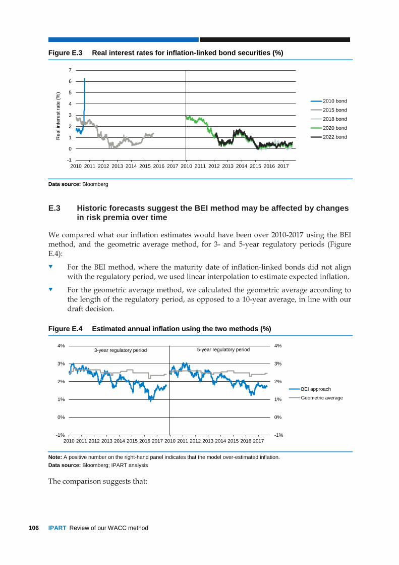
106 IPART Review of our WACC method
Figure E.3 Real interest rates for inflation-linked bond securities (%)
Data source: Bloomberg
E.3 Historic forecasts suggest the BEI method may be affected by changes in risk premia over time
We compared what our inflation estimates would have been over 2010-2017 using the BEI
method, and the geometric average method, for 3- and 5-year regulatory periods (Figure E.4):
For the BEI method, where the maturity date of inflation-linked bonds did not align
with the regulatory period, we used linear interpolation to estimate expected inflation.
For the geometric average method, we calculated the geometric average according to
the length of the regulatory period, as opposed to a 10-year average, in line with our
draft decision.
Figure E.4 Estimated annual inflation using the two methods (%)
Note: A positive number on the right-hand panel indicates that the model over-estimated inflation.
Data source: Bloomberg; IPART analysis
The comparison suggests that:
-1
0
1
2
3
4
5
6
7
2010 2011 2012 2013 2014 2015 2016 2017 2010 2011 2012 2013 2014 2015 2016 2017
2010 bond
2015 bond
2018 bond
2020 bond
2022 bondRe
al in
tere
st ra
te (
%)
-1%
0%
1%
2%
3%
4%
-1%
0%
1%
2%
3%
4%
2010 2011 2012 2013 2014 2015 2016 2017 2010 2011 2012 2013 2014 2015 2016 2017
BEI approach
Geometric average
3-year regulatory period 5-year regulatory period

Review of our WACC method IPART 107
The forecasts using the geometric average would have only fallen slightly over the
2010-2017 period (the grey lines). Inflation rates using this approach would have been
between 2.3-2.4% in recent years.
Expected inflation using the BEI method is currently around 1.7-1.8% for this period (the blue lines).
The BEI method produced expected inflation rates in the middle of 2016 of around
1.0%. This reflects that real interest rates were around 0.4% in this period, and nominal interest rates were about 1.4%.
Figure E.5 charts the difference between actual CPI inflation and the inflation estimates
produce by each method over the period 2010 to 2017. A positive number indicates that the method would have over-estimated inflation:
The data for 2010-2012 suggests neither the geometric average and the BEI method
initially predicted the low inflation environment that we subsequently entered into, and therefore over-estimated inflation.
Over a 3-year period (left-hand panel), the BEI method would have produced slightly
smaller forecast errors than a geometric average method.
Over a 5-year period (right-hand panel), there is less evidence the BEI method is more
accurate than a geometric average method.
Figure E.5 Realised forecast errors using the two methods (%)
Note: A positive number on the right-hand panel indicates that the model over-estimated inflation.
Data source: Bloomberg; IPART analysis
Based on the analysis summarised in Figure E.1 to Figure E.5, our overall conclusion is that:
The geometric average approach would over-estimate inflation in the current low
inflation environment. However, to the extent that future inflation is uncertain, our method should gravitate towards an average expected inflation rate over the longer
term. As outlined in our Issues Paper, our view is that long-term inflation
expectations are anchored around the midpoint of the RBA’s inflation target band (2.5%).206 Therefore, we consider a geometric average method approximates the
average inflation rate over time.
206 IPART, Review of WACC methodology, Issues Paper, July 2017, p 44.
-0.5%
0.0%
0.5%
1.0%
1.5%
2.0%
-0.5%
0.0%
0.5%
1.0%
1.5%
2.0%
2010 2011 2012 2013 2014 2015 2016 2017 2010 2011 2012 2013 2014 2015 2016 2017
BEI approach
Geometric average
3-year regulatory period 5-year regulatory period

108 IPART Review of our WACC method
The accuracy of the BEI method may be impacted over time to the extent that the risk
premia affecting the yield on inflation-linked bonds, such as liquidity risk, vary at
different points in the economic cycle.
E.4 The geometric average method is simpler, more transparent and replicable
The geometric average approach uses data that is publicly available and directly observable. The RBA currently produces semi-annual inflation forecasts in its quarterly SMP. The only
drawback with this approach is that there is not an inflation forecast that is exactly 1-year
ahead at all points in time. For example, stakeholders may be unclear whether we used a 9-month ahead, or 15-month ahead inflation forecast. Our final decision would define our 1-
year ahead inflation forecast more precisely.
The smaller amount of inflation-linked bond issuance results in data limitations. As a consequence, more judgement would be required to estimate inflation using the BEI
method. To estimate inflation with the BEI method, we would need to:
1. Determine what time period we collect bond market data to estimate inflation.
2. Ascertain whether there is an inflation-linked bond with a maturity equal to the
regulatory period.
3. If there is, calculate expected inflation directly using the fisher equation.
4. If not, interpolate an expected inflation rate consistent with the regulatory period,
using inflation linked bonds of similar maturity. This would involve:
– deciding a method we would use to interpolate an expected inflation rate, and
– potentially ignoring data from inflation linked bonds with a short maturity,
which may be affected by illiquidity.
The bond yield data used to calculate inflation using the BEI method is publicly available through the RBA website. However, as judgement is required to estimate inflation using
this method, we consider that the BEI method would be more difficult for stakeholders to
replicate.