Review of HAARP Experiment and Assessment of Ionospheric ......Third ALOS PI Symposium Kona, Hawaii...
29
Third ALOS PI Symposium Kona, Hawaii November 9-13, 2009 Review of HAARP Experiment and Assessment of Ionospheric Effects T. L. Ainsworth 1 , Y. Wang 1 , J.-S. Lee 1,2 and K.-S. Chen 2 1 Naval Research Laboratory, Washington DC, USA 2 CSRSR, National Central University, TN (ROC)
Transcript of Review of HAARP Experiment and Assessment of Ionospheric ......Third ALOS PI Symposium Kona, Hawaii...
Third ALOS PI Symposium Kona, Hawaii
November 9-13, 2009
Review of HAARP Experiment and
Assessment of Ionospheric Effects
T. L. Ainsworth1, Y. Wang1, J.-S. Lee1,2
and K.-S. Chen2
1Naval Research Laboratory, Washington DC, USA2CSRSR, National Central University, TN (ROC)

2
Objectives
•
Determine ionospheric effects on PALSAR polarimetry
•
Develop ionosphere correction methods
–
Faraday rotation compensation
•
Assess required compensation tolerances
–
Based on desired polarimetric capabilities
•
Employ SAR to measure ionosphere properties
–
High resolution ionospheric measurements

3
TEC Effects on SAR
( )∫≈path
electron xdxnTEC
Sat
ellit
e A
ltitu
de ~
700k
m
Ionosphere F2 Layer Alt. ~300km
First-Order Effects on Pol. SAR:
•
Faraday Rotation ∝
TEC Value
•
Azimuth Shifts ∝
TEC Gradient
Total Electron Content,
θ
TEC Varies Diurnally and with Solar Sunspot Cycle
Ionosphere TEC Causes
•
Refraction, θ
•
Faraday Rotation

4
HAARP Experiment Concept
•
Generate artificial “TEC hole”
in ionosphere–
Use HAARP high power HF transmitter
•
Frequency: 3-10 MHz, Max Power: ~3.6 Mw
•
Synchronize with PALSAR quad-pol collect –
Image through artificially disturbed ionosphere
•
Compare with ionosphere electron density –
Ground based measurements
–
Tomographic
electron density information
High-frequency Active Auroral
Research Program

5
Observational Difficulties
•
Coordination of experimental conditions–
HAARP HF radar schedule
–
PALSAR quad-pol imagery collects
–
Naturally occurring phenomena•
Sufficient TEC levels
•
Solar activity affects the ionosphere–
Near the minimum of the 11 year solar cycle
•
Primary problems: –
Insufficient electron density
–
Limited observational opportunities

6
Opportunistic Observations
•
Naturally occurring ionospheric irregularity
•
Serendipity, or
•
Choose a good location –
Frequent ionosphere disturbances
•
Sufficient TEC variability
–
Frequent PALSAR quad-pol collects
–
Complementary, ground based dataset•
E.g. TEC / electron density mapping
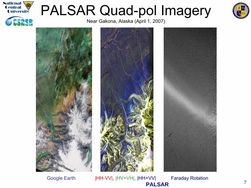
7Google Earth |HH-VV|, |HV+VH|, |HH+VV| Faraday Rotation
PALSAR
PALSAR Quad-pol ImageryNear Gakona, Alaska (April 1, 2007)

8
Tomographic
Imaging Data
Ionosphere measurements taken at HAARP show spatial and day-to-day electron density variability
Quiet Day
31 March 2007; 0718 –
0736 UTC
59 62 65 68 71
Geomagnetic Latitude Nelec
[1011
e/m3]
Disturbed Day
1 April 2007; 0757 –
0814 UTC
59 62 65 68 71
Geomagnetic Latitude Nelec
[1011
e/m3]
High-frequency Active Auroral Research Program

9Faraday Rotation
Azimuth Profile of Faraday Rotation
Irregularity
Mean = 2.98127°
Polarimetric Faraday Effect

10
Observational Outlook
•
Better opportunities in the near-term–
Solar cycle is (should be) heading toward a maximum•
Increased free electron density –
increased TEC
•
Increased TEC variability
•
Opportunistic ionosphere observations –
Good solution at specific test sites•
Assuming routine quad-pol image collection
•
HAARP concept is feasible provided–
Well coordinated data collection plan•
PALSAR quad-pol imagery, HAARP HF radar, etc.

11
Faraday Compensation
How much does TEC affect SAR polarimetry?
•
Assess polarimetric effects on derived products
•
Treat Faraday rotations as a miscalibrations
•
Can one compensate dual-pol imagery?
uncompensated

12
Faraday Effects
•
Faraday rotation affects polarimetric calibration
–
Generates non-reciprocal SAR returns
–
Circular basis: Phase of RL·LR* correlation
•
Non-unique cross-talk / Faraday separation
–
Cross-talk induces non-reciprocal returns •
Affects RL·LR* correlations
–
PALSAR: cross-talk level not an issue

13
Faraday Rotation Estimation
⎥⎦
⎤⎢⎣
⎡ΩΩ−ΩΩ
⎥⎦
⎤⎢⎣
⎡⎥⎦
⎤⎢⎣
⎡ΩΩ−ΩΩ
=⎥⎦
⎤⎢⎣
⎡cossinsincos
cossinsincos
vvhv
hvhh
vvvh
hvhh
SSSS
OOOO
•
Estimate
Faraday rotation, Ω, in the circular basis–
Well-defined –
based on second-order statistics–
Insensitive to target orientation angles –
Insensitive to scattering mechanisms in the scene
)]([21
vvhhvhhvRL OOjOOO ++−=
)]([21
vvhhhvvhLR OOjOOO ++−=
( )444
1 ππ≤Ω≤−−=Ω with*
LRRLOOArg

14
Faraday Rotation Matrix
where γ
= tan Ω, and Ω
is the Faraday rotation angle
⎥⎥⎥⎥⎥⎥
⎦
⎤
⎢⎢⎢⎢⎢⎢
⎣
⎡
⎥⎥⎥⎥⎥⎥
⎦
⎤
⎢⎢⎢⎢⎢⎢
⎣
⎡
−−
−−
−−
∝
⎥⎥⎥⎥⎥⎥
⎦
⎤
⎢⎢⎢⎢⎢⎢
⎣
⎡
⎥⎥⎥⎥⎥⎥
⎦
⎤
⎢⎢⎢⎢⎢⎢
⎣
⎡
ΩΩΩΩΩ−Ω−
ΩΩ−ΩΩΩΩ−
ΩΩΩΩΩΩ
Ω−ΩΩΩΩ−Ω
=
⎥⎥⎥⎥⎥⎥
⎦
⎤
⎢⎢⎢⎢⎢⎢
⎣
⎡
VV
VH
HV
HH
VV
VH
HV
HH
VV
VH
HV
HH
S
S
S
S
S
S
S
S
O
O
O
O
1
1
1
1
cossincossincossin
sincoscossinsincos
sincossincossincos
sinsincossincoscos
2
2
2
2
22
22
22
22
γγγ
γγγ
γγγ
γγγ
⎥⎦
⎤⎢⎣
⎡ΩΩ−ΩΩ
⎥⎦
⎤⎢⎣
⎡⎥⎦
⎤⎢⎣
⎡ΩΩ−ΩΩ
=⎥⎦
⎤⎢⎣
⎡cossinsincos
cossinsincos
vvhv
hvhh
vvvh
hvhh
SSSS
OOOO

15
⎥⎦
⎤⎢⎣
⎡⎥⎦
⎤⎢⎣
⎡ΩΩ−Ω+Ω
⎥⎦
⎤⎢⎣
⎡⎥⎦
⎤⎢⎣
⎡ΩΩ−Ω+Ω
⎥⎦
⎤⎢⎣
⎡=⎥
⎦
⎤⎢⎣
⎡
VVVH
HVHH
VVVH
HVHH
VVVH
HVHH
VVVH
HVHH
tttt
SSSS
rrrr
OOOO
cossinsincos
cossinsincos
⎥⎥⎥⎥
⎦
⎤
⎢⎢⎢⎢
⎣
⎡
⎥⎥⎥⎥⎥
⎦
⎤
⎢⎢⎢⎢⎢
⎣
⎡
−−
−−−−
⎥⎥⎥⎥
⎦
⎤
⎢⎢⎢⎢
⎣
⎡
⎥⎥⎥⎥
⎦
⎤
⎢⎢⎢⎢
⎣
⎡
∝
⎥⎥⎥⎥
⎦
⎤
⎢⎢⎢⎢
⎣
⎡
−−
−
VV
VH
HV
HH
VV
VH
HV
HH
SSSS
k
k
zuuzvuvuwwzzvwwv
OOOO
11
11
11
11
2
2
2
2
11
1
γγγγγγγγγγγγ
αα
αα
Full Calibration Model
where γ
= tan Ω, and Ω
is the Faraday rotation angle
Faraday rotations
destroy diagonal dominance of the [X][G][F] calibration matrix. γ
is not necessarily a small parameter.
X-talk, [X] Gain, [G] Faraday, [F]
T.L. Ainsworth, L. Ferro-Famil & J.-S. Lee, TGRS, vol. 44, 2006, pp. 994-1003.

16
Faraday Rotations
( )[ ]
⎥⎥⎥⎥⎥
⎦
⎤
⎢⎢⎢⎢⎢
⎣
⎡
−−
−−
−−
∝Ω
1
1
1
1
2
2
2
2
γγγ
γγγ
γγγ
γγγ
F
where γ
= tan Ω, and Ω
is the Faraday rotation angle
•
Faraday rotation and cross-talk matrices are similar
•
Faraday rotations affect cross-talk calibration−
Setting z = -u = -v = w and cross-talk generates “Faraday rotation”
[ ]⎥⎥⎥⎥
⎦
⎤
⎢⎢⎢⎢
⎣
⎡
∝
11
11
zuuzvuvuwwzzvwwv
X
where u, v, w
and z
are the cross-talk coefficients
Cross-talk MatrixFaraday Rotation Matrix

17
Generic Error Metrics
•
Metrics should be simple
•
Similar metrics for point and distributed targets
–
Point targets metrics
•
Apply to scattering matrix formalism
–
Distributed target metrics
•
Apply to covariance / coherency matrices

18
Point Target Error Metric•
Define a point target metric to assess impacts of Faraday rotations and other polarization errors
( )Ω= FD( )( ) ( )
( )2
2
2
2
t
t
St
S SSID
Se
tt vecvec
maxvec
max−
=
Seek for the maximum normalized errors in the target space:
Evaluated as the induced norm:
( ) ( ) ( )( )
2
22
t
t4
S4 SSAID
AIDt vec
vecmax
−=−
Canonical targets display reciprocal scattering.Observations are not reciprocal due to Faraday rotations.
( )( ) ( )
( )2
2
2
2
t
t4
St
S SSAID
Se
tt vecvec
maxvec
max−
=⎥⎥⎥⎥
⎦
⎤
⎢⎢⎢⎢
⎣
⎡
=
1000
02121
0
0001
4A
Faraday correction

19
Evaluation•
The defined metric is used to evaluate the compromised polarimetric accuracy due to Faraday rotation.–
Worst case situation: quad-pol and several dual-pol modes
( )Ω− 212 cos
20
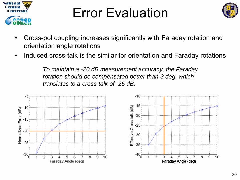
Error Evaluation
•
Cross-pol coupling increases significantly with Faraday rotation and orientation angle rotations
•
Induced cross-talk is the similar for orientation and Faraday rotations
To maintain a -20 dB measurement accuracy, the Faraday rotation should be compensated better than 3 deg, which translates to a cross-talk of -25 dB.

21
Distributed Target Metric•
Polarization synthesis determines the maximum error for all allowed combinations of transmitted and received polarizations
•
Synthesis bias is obtained from a general eigen problem,
–
where A4
restricts error maximization to reciprocal scattering
( )( ) ( )
( )vvmaxvv
vvmax HHH
vAΣAvHH
HHH
tHH 44
144
44
44
ADDΣAAΣAADDΣA
tt
t
==
This error metric represents a worst case scenario.
[ ] basis V)(H, linear
⎥⎥⎥⎥⎥
⎦
⎤
⎢⎢⎢⎢⎢
⎣
⎡
∝
3001
0110
0110
1003
volumeC

22
Polarization SynthesisPredicted synthesis errors for typical natural targets.
⎥⎥⎥⎥
⎦
⎤
⎢⎢⎢⎢
⎣
⎡
−
−−
977130097
130150140
097140976
57130
571452
30452
.e.e.
e..e.
e.e..
oo
oo
oo
.j.j
.j.j
.j.j
⎥⎥⎥⎥
⎦
⎤
⎢⎢⎢⎢
⎣
⎡
−−
−
721180182
180170360
182360865
8146164
8144133
61644133
.e.e.
e..e.
e.e..
oo
oo
oo
.j.j
.j.j
.j.j
⎥⎥⎥⎥
⎦
⎤
⎢⎢⎢⎢
⎣
⎡
−
−
−
132070640
070841160
640160383
0102615
01027113
6157113
.e.e.
e..e.
e.e..
oo
oo
oo
.j.j
.j.j
.j.j
Sample covariance matrices drawn from PALSAR imagery
Urban Target

23
Pauli Basis Effects
Only the surface scattering component is affected.
Overall, the Pauli decomposition shows little change.
Pauli Display: Ω
= 0°
Pauli Display: Ω
= 10°
Double Bounce
|HH-VV|/√2 (dB)
Surface
|HH+VV|/√2 (dB)
Ω = 10°
|HH-VV|
|HV+VH|
|HH+VV|

24
Pauli Basis Effects
Only the surface scattering component is affected.
Overall, the Pauli decomposition shows little change.
Pauli Display: Ω
= 0°
Pauli Display: Ω
= 20°|HH-VV|/√2 (dB)
Double Bounce
|HH+VV|/√2 (dB)
Surface
Ω = 20°
|HH-VV|
|HV+VH|
|HH+VV|

25
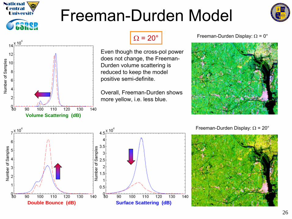
Freeman-Durden Model
Even though the cross-pol power does not change, the Freeman-
Durden volume scattering is reduced to keep the model positive semi-definite.
Overall, Freeman-Durden shows more yellow, i.e. less blue.
Freeman-Durden Display: Ω
= 0°
Freeman-Durden Display: Ω
= 10°
Volume Scattering (dB)
Double Bounce (dB) Surface Scattering (dB)
Ω = 10°
26
Freeman-Durden ModelFreeman-Durden Display: Ω
= 0°
Freeman-Durden Display: Ω
= 20°
Even though the cross-pol power does not change, the Freeman-
Durden volume scattering is reduced to keep the model positive semi-definite.
Overall, Freeman-Durden shows more yellow, i.e. less blue.
Volume Scattering (dB)
Double Bounce (dB) Surface Scattering (dB)
Ω = 20°

27
Conclusions
•
Quad-pol PALSAR data provides precise Faraday rotation estimates–
L-band quad-pol imagery can be polarimetrically calibrated in the presence of Faraday rotations
•
Faraday effects on PALSAR polarimetry –
Surface scattering shows greatest effect, i.e. |HH+VV|–
Quad-pol imagery •
Appears to tolerate up to ~10°
of uncompensated Faraday rotation–
Freeman-Durden classification comparison–
Standard distributed targets analysis
•
Quad-pol easily compensated for Faraday rotations
–
Dual-pol imagery•
Circular transmit modes display smallest Faraday effects •
Linear transmit dual-pol modes strongly effected –
Especially for surface and double bounce scattering –
Linear dual-pol modes require better Faraday compensation

28
Thank you

29
Orientation Angle
( )[ ]
⎥⎥⎥⎥⎥
⎦
⎤
⎢⎢⎢⎢⎢
⎣
⎡
ΓΓΓΓ−Γ−ΓΓ−Γ−Γ
ΓΓ−Γ−
∝
⎥⎥⎥⎥⎥
⎦
⎤
⎢⎢⎢⎢⎢
⎣
⎡
−−−−
−−
=
11
11
2
2
2
2
22
22
22
22
θθθθθθθθθθθθθθθθθθ
θθθθθθ
θ
cossincossincossinsincoscossinsincossincossincossincos
sinsincossincoscos
R
where Γ
= tan θ, and θ
is the orientation angle, a rotation about the line of sight.
Rotation, Faraday and Cross-talk matrices have similar forms
( )[ ]⎥⎥⎦
⎤
⎢⎢⎣
⎡
+
−
⎥⎥⎦
⎤
⎢⎢⎣
⎡
⎥⎥⎦
⎤
⎢⎢⎣
⎡
−
+=
θθ
θθ
θθ
θθθ
cossin
sincos
SS
SS
cossin
sincosS
VVVH
HVHH
[ ]⎥⎥⎥⎥
⎦
⎤
⎢⎢⎢⎢
⎣
⎡
∝
11
11
zuuzvuvuwwzzvwwv
X( )[ ]
⎥⎥⎥⎥⎥
⎦
⎤
⎢⎢⎢⎢⎢
⎣
⎡
ΓΓΓ
Γ−Γ−Γ
Γ−Γ−Γ
ΓΓ−Γ−
∝
1
1
1
1
2
2
2
2
θR ( )[ ]
⎥⎥⎥⎥⎥
⎦
⎤
⎢⎢⎢⎢⎢
⎣
⎡
−−
−−
−−
∝Ω
1
1
1
1
2
2
2
2
γγγ
γγγ
γγγ
γγγ
F
Rotation Faraday Cross-talk


![DEMETER observations of the ionospheric trough over HAARP ... · [9] DEMETER is a low Earth orbit satellite with an alti-tude of approximately 670 km, inclination of 98.3° and horizontal](https://static.fdocuments.in/doc/165x107/5fda6cce888b7679ed176d03/demeter-observations-of-the-ionospheric-trough-over-haarp-9-demeter-is-a-low.jpg)