Review of Error Analysis and Practice Problems for PHY 201L/211L

Review of Error Analysis and Practice Problems for

PHY 201L/211L

and

PHY 202L/212L

General College/University Physics Lab

Barry University

Physical Sciences Department

Contents

1 Error Analysis 31.1 The Meaning of Error in Science . . . . . . . . . . . . . . . . . . . . . . . . . . . . . 31.2 Importance in Understanding Errors . . . . . . . . . . . . . . . . . . . . . . . . . . . 31.3 Reporting Errors . . . . . . . . . . . . . . . . . . . . . . . . . . . . . . . . . . . . . . 4

2 Propagation of Errors 52.1 Error of the Sum and Difference of two Measured Quantities . . . . . . . . . . . . . 52.2 Error in the Product of two Measured Quantities . . . . . . . . . . . . . . . . . . . . 52.3 Error in the power of a Measured Quantity . . . . . . . . . . . . . . . . . . . . . . . 52.4 Error of the Quotient of two Measured Quantities . . . . . . . . . . . . . . . . . . . . 62.5 Errors in Composed Expressions . . . . . . . . . . . . . . . . . . . . . . . . . . . . . 6

3 Graphics 73.1 Graphical Analysis . . . . . . . . . . . . . . . . . . . . . . . . . . . . . . . . . . . . . 73.2 Microsoft Excel . . . . . . . . . . . . . . . . . . . . . . . . . . . . . . . . . . . . . . . 83.3 Error associated with the slope . . . . . . . . . . . . . . . . . . . . . . . . . . . . . . 10

4 General Problems on the Calculation of the Uncertainties 114.1 Proper rounding and proper units . . . . . . . . . . . . . . . . . . . . . . . . . . . . 114.2 Propagation of errors . . . . . . . . . . . . . . . . . . . . . . . . . . . . . . . . . . . . 114.3 Other problems on propagation of errors . . . . . . . . . . . . . . . . . . . . . . . . . 12

5 Problems On Graphing 13

6 Problems on Basic Kinematics and Dynamics 196.1 Kinematics . . . . . . . . . . . . . . . . . . . . . . . . . . . . . . . . . . . . . . . . . 196.2 Acceleration due to gravity . . . . . . . . . . . . . . . . . . . . . . . . . . . . . . . . 196.3 Newton’s law . . . . . . . . . . . . . . . . . . . . . . . . . . . . . . . . . . . . . . . . 206.4 Linear momentum . . . . . . . . . . . . . . . . . . . . . . . . . . . . . . . . . . . . . 216.5 Rigid bodies . . . . . . . . . . . . . . . . . . . . . . . . . . . . . . . . . . . . . . . . . 21

7 Problems on Waves and Sound 23

8 Problems on Thermodynamics 24

9 Problems on DC-Circuits 259.1 Ohm’s law . . . . . . . . . . . . . . . . . . . . . . . . . . . . . . . . . . . . . . . . . . 259.2 Diodes . . . . . . . . . . . . . . . . . . . . . . . . . . . . . . . . . . . . . . . . . . . . 269.3 Parallel and series of resistors and Kirchhoff’s rules . . . . . . . . . . . . . . . . . . . 279.4 RC-circuits . . . . . . . . . . . . . . . . . . . . . . . . . . . . . . . . . . . . . . . . . 29

10 Problems on Resonant Circuits 31

11 Problems on the Oscilloscope 32

12 Problems on Magnetic Field 33

13 Problems on Electromagnetic Waves and Optics 34

2

1 Error Analysis

1.1 The Meaning of Error in Science

In science, the term error does not carry the negative connotation of the term mistake. Everyscientific measurement is subject to errors, and the role of the scientist is to understand andquantify them (since you cannot avoid them, learn how to deal with them).

Let us start with a discussion of some of the possible sources of errors in a scientific experiment:

• Precision: This term refers to how fine the measurement scale is. For example, a rulerwhich reports millimeters is more precise that one which reports only centimeters. However,no instrument we use for measuring is perfect. As a thumb rule, the precision of an instrumentis taken to be half the minimal increment that the instrument can measure. For example, isa scale reports grams as its minimal unit, the precision of that scale is taken to be 0.5 grams.

• Random Errors: These types of errors produce measurements that are randomly a littlehigher or a little lower than the true value of the quantity we are measuring. There aredifferent sources of random errors. An example is the measurement error refers to our abilityto perform the measurement. This can mean, for example, our ability to stop a watch at theright time. On the other hand, the intrinsic random uncertainty refers to random sourcesof error which are not connected with our ability, but are due to uncontrollable physicaleffects such as thermal or electromagnetic fluctuations, random noise, etc. In precision mea-surements, also quantum fluctuations could be a source for errors. If these fluctuations arerandom, then they are also considered random errors.

• Systematic Errors: These kinds of errors are due to non-random effects which produce anerror in the measurement. For example, a slow watch would measure the wrong time even ifwe were very careful. Another example could be the use of the wrong value for a parameterneeded in the measurement.

Another difficulty associated with a measurement is the so called problem of definition [see,e.g., Taylor (1997)1]. Suppose we want to measure a rectangular piece of wood. The size of thepiece changes with temperature, humidity, etc. So it is important to specify what we mean by size(size at what temperature and humidity?) if the measurement aims to be accurate enough to besensitive to those temperature and humidity conditions.

1.2 Importance in Understanding Errors

In some cases it does not seem necessary to understand the errors very much. When we plan a cartrip we are not interested in knowing the distance to the accuracy of 1 foot.

In certain cases, however, it is very important to understand the uncertainty associated witha measurement. Suppose, for example, that a police officer has a very rudimentary instrument todetect the velocity of cars, which is accurate at the level of 10 miles per hour. Suppose that on astreet the speed limit is 35 miles per hour and he stops a car which, according to his instrument,is going 40 miles/hour. Because of the imprecision of his instrument, the actual car velocity issomewhere between 30 and 50 miles/hour, so the officer cannot really give a ticket to the driver (ifhe knows the error associated with this measurement). If, instead, his instrument has an accuracy of

1John Taylor, An Introduction to Error Analysis: The Study of Uncertainties in Physical Measurements, UniversityScience Books; 2nd edition (March 1997).

3

1 mile/hour, then the agent could conclude that the car was speeding since its velocity is somewherebetween 39 and 41 miles/hour.

1.3 Reporting Errors

The standard way to present the result of a measurement in a scientific report is

x±∆x , or x± δx , (1.1)

which means Measured Value ± Uncertainty. Notice that both notations, ∆ and δ, are used in theliterature, and in this manual we will also use both symbols to indicate the uncertainty2.

The uncertainty can be associated with the imperfection of the measuring instrument or withother effects, as explained above. Ideally, it would be useful to explain the source of uncertainty inthe experiment report.

When we write the result of our measure in the form above, ∆x should be rounded to onesignificant figure, except when the leading digit in the uncertainty is 1. In fact, it does not makesense to say that the uncertainty is, for example, 5.145 since 0.145 is a small correction to theleading digit 5. However, if, for example, we find ∆x = 1.4, it would be a good idea to report thesecond digit, since 0.4 is not really negligible with respect to 1. In addition, the last significant figurein x should be of the same order of magnitude (in the same decimal position) as the uncertainty.For example, 11.3 ± 5 does not make much sense. In fact, since the error is 5, it is not useful toreport also the decimal figure in our result. The correct form is 11 ± 5. Other correct examplesare: 110 ± 30, 11.3 ± 0.2, and 1905 ± 2.

Problem: Which of the following are correct ways to report the value of a measurement of alength?

a. (110 ± 10) mb. (110 ± 11.2) mc. (110 ± 1) md. (8.33 ± 1) me. (833.765 ± 0.005) m

2The symbol ∆ (read delta) indicates a capital D in the Greek alphabet, and δ indicates a small d.

4

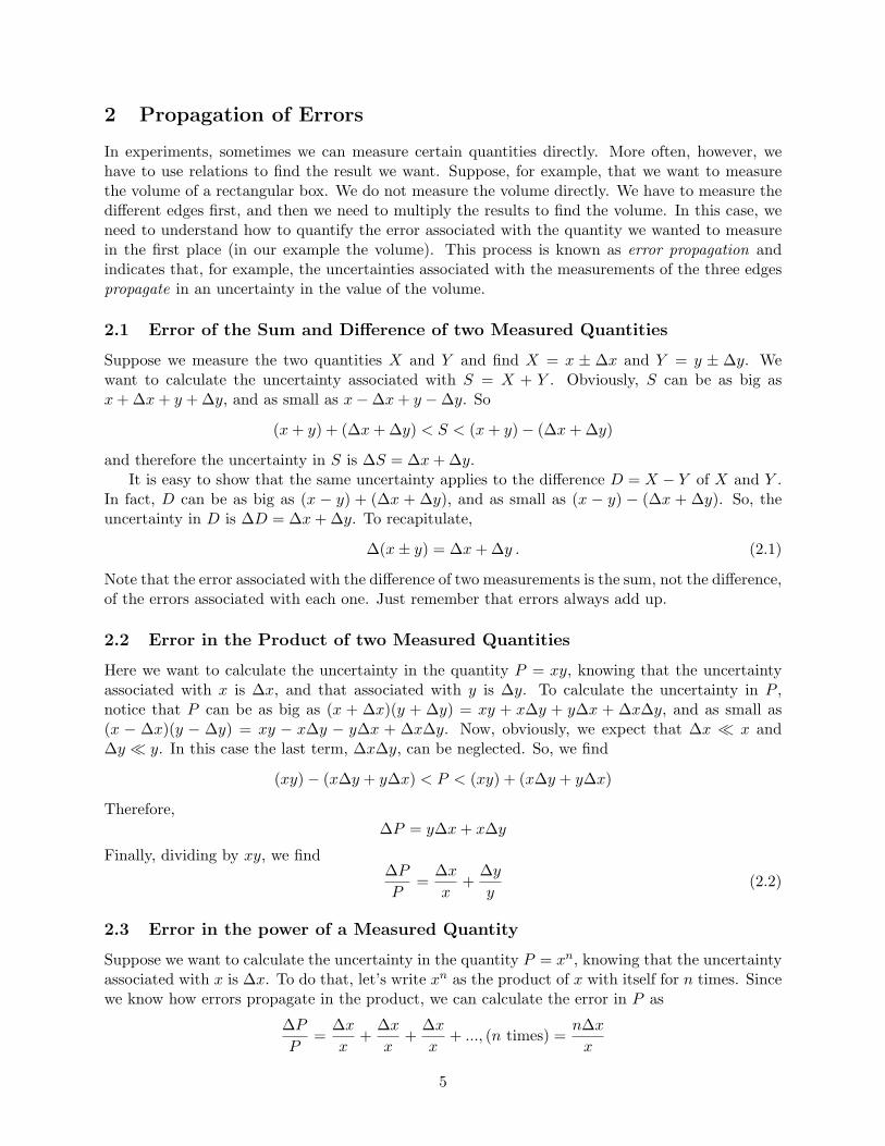
2 Propagation of Errors

In experiments, sometimes we can measure certain quantities directly. More often, however, wehave to use relations to find the result we want. Suppose, for example, that we want to measurethe volume of a rectangular box. We do not measure the volume directly. We have to measure thedifferent edges first, and then we need to multiply the results to find the volume. In this case, weneed to understand how to quantify the error associated with the quantity we wanted to measurein the first place (in our example the volume). This process is known as error propagation andindicates that, for example, the uncertainties associated with the measurements of the three edgespropagate in an uncertainty in the value of the volume.

2.1 Error of the Sum and Difference of two Measured Quantities

Suppose we measure the two quantities X and Y and find X = x ± ∆x and Y = y ± ∆y. Wewant to calculate the uncertainty associated with S = X + Y . Obviously, S can be as big asx+ ∆x+ y + ∆y, and as small as x−∆x+ y −∆y. So

(x+ y) + (∆x+ ∆y) < S < (x+ y)− (∆x+ ∆y)

and therefore the uncertainty in S is ∆S = ∆x+ ∆y.It is easy to show that the same uncertainty applies to the difference D = X − Y of X and Y .

In fact, D can be as big as (x − y) + (∆x + ∆y), and as small as (x − y) − (∆x + ∆y). So, theuncertainty in D is ∆D = ∆x+ ∆y. To recapitulate,

∆(x± y) = ∆x+ ∆y . (2.1)

Note that the error associated with the difference of two measurements is the sum, not the difference,of the errors associated with each one. Just remember that errors always add up.

2.2 Error in the Product of two Measured Quantities

Here we want to calculate the uncertainty in the quantity P = xy, knowing that the uncertaintyassociated with x is ∆x, and that associated with y is ∆y. To calculate the uncertainty in P ,notice that P can be as big as (x + ∆x)(y + ∆y) = xy + x∆y + y∆x + ∆x∆y, and as small as(x − ∆x)(y − ∆y) = xy − x∆y − y∆x + ∆x∆y. Now, obviously, we expect that ∆x x and∆y y. In this case the last term, ∆x∆y, can be neglected. So, we find

(xy)− (x∆y + y∆x) < P < (xy) + (x∆y + y∆x)

Therefore,∆P = y∆x+ x∆y

Finally, dividing by xy, we find∆PP

=∆xx

+∆yy

(2.2)

2.3 Error in the power of a Measured Quantity

Suppose we want to calculate the uncertainty in the quantity P = xn, knowing that the uncertaintyassociated with x is ∆x. To do that, let’s write xn as the product of x with itself for n times. Sincewe know how errors propagate in the product, we can calculate the error in P as

∆PP

=∆xx

+∆xx

+∆xx

+ ..., (n times) =n∆xx

5

An interesting fact is that this formula is always valid, even if n is not positive or not integer.In general we have that, if P = xn,

∆PP

=|n|∆xx

(2.3)

where |n| is the absolute value of n.

Problem: Use this formula to find the error associated with the square root of a quantity.

Solution: ∆ (√x) = ∆

(x1/2

)= 1

2

√x(

∆xx

)2.4 Error of the Quotient of two Measured Quantities

Consider, finally, the quantity Q = x/y, where the uncertainty in x is ∆x and in y is ∆y. We cancalculate the uncertainty associated with Q, by writing Q = xy−1, and using the previous resultsfor the uncertainty associated with the product and with the power: Dividing x by y we find:

∆(xy−1)xy−1

=∆xx

+ | − 1|∆yxy

which means∆QQ

=∆xx

+∆yy

(2.4)

2.5 Errors in Composed Expressions

Some expressions are combinations of sums or a products. In this case we can use the chain ruleto find how errors propagate. For example, suppose we want to calculate the uncertainty in theexpression

x3 + y2 , (2.5)

knowing that the uncertainty in x is δx, and the uncertainty in y is δy.First of all, we note that the expression indicates a sum of x3 and y2. So, the first step is

δ(x3 + y2) = δ(x3) + δ(y2) . (2.6)

Now, each of the expressions represents a power. We can expand each of them and get

δ(x3) + δ(y2) = x3

(3δx

x

)+ y2

(2δy

y

)= 3x2 δx+ 2y δy . (2.7)

So, the result isδ(x3 + y2) = 3x2 δx+ 2y δy . (2.8)

6

3 Graphics

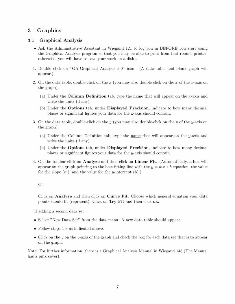
3.1 Graphical Analysis

• Ask the Administrative Assistant in Wiegand 121 to log you in BEFORE you start usingthe Graphical Analysis program so that you may be able to print from that room’s printer-otherwise, you will have to save your work on a disk).

1. Double click on ”GA-Graphical Analysis 3.0” icon. (A data table and blank graph willappear.)

2. On the data table, double-click on the x (you may also double click on the x of the x-axis onthe graph).

(a) Under the Column Definition tab, type the name that will appear on the x-axis andwrite the units (if any).

(b) Under the Options tab, under Displayed Precision, indicate to how many decimalplaces or significant figures your data for the x-axis should contain.

3. On the data table, double-click on the y (you may also double-click on the y of the y-axis onthe graph).

(a) Under the Column Definition tab, type the name that will appear on the y-axis andwrite the units (if any).

(b) Under the Options tab, under Displayed Precision, indicate to how many decimalplaces or significant figures your data for the y-axis should contain.

4. On the toolbar click on Analyze and then click on Linear Fit. (Automatically, a box willappear on the graph pointing to the best fitting line with the y = mx+ b equation, the valuefor the slope (m), and the value for the y-intercept (b).)

or..

Click on Analyze and then click on Curve Fit. Choose which general equation your datapoints should fit (represent). Click on Try Fit and then click ok.

If adding a second data set

• Select ”New Data Set” from the data menu. A new data table should appear.

• Follow steps 1-3 as indicated above.

• Click on the y on the y-axis of the graph and check the box for each data set that is to appearon the graph.

Note: For further information, there is a Graphical Analysis Manual in Wiegand 148 (The Manualhas a pink cover).

7

3.2 Microsoft Excel

(adapted from www.brighthub.com)

Step 1: Enter or copy/paste your data into an Excel worksheet.As an example in this tutorial, we’ll be using data consisting ofhours spent studying and final exam scores for a select group ofstudents.

Step 2: Highlight the columns that contain the data you want torepresent in the scatter plot. In this example, those columns areHours Spent Studying and Exam Score.

Step 3: Open the Insert tab on the Excel ribbon. Click on Scatterin the Charts section to expand the chart options box. Select thefirst item, Scatter with only Markers, from this box. After makingthis selection, the initial scatter plot will be created in the sameworksheet. You can resize this chart window and drag it to anyother part of the worksheet.

Step 4: Make any formatting or design changes you wish in theDesign, Layout, and Format tabs located under Chart Tools onthe Excel ribbon. For example, every graph need axes labels withunits, and a title.

8

Label the Axes: Horizontal axis: select the Layout tab underChart Tools. Next, click on Axis Titles in the Labels section.Choose Primary Horizontal Axis and then pick Title Below Axis.A text box with the default wording Axis Title will appear on thechart. Click anywhere in that text box and edit the informationto reflect the true title of the horizontal axis.Similarly, you can create a label for the vertical axis, but you willhave more choices for title placement here. You’ll need to use theRotated Title option.Chart Legend: The default legend that was created with thescatter plot serves no real purpose here, so you can get rid of it.Go back to the Layout tab and click on Legend. From the listof expanded options, pick None to turn off the legend. Now yourchart should now look like the one in the screenshot on the right.

Change Chart Title: Click on the title to open the text boxthat contains it and edit it with your new description.

Add a Trendline: Adding a trendline asks the computer to drawthe best line of fit through your experimental data. You can in-clude the equation for that line, which will have the general formy = mx+ b.Right-click on any point on your graph, and select Add Trend-line from the menu that appears. Select Linear and make surethe boxes Display Equation on chart and Display R-squaredvalue on chart are selected.If there is a point in your data that must have a value of 0 forboth variables (x and y), you can place a check mark next to SetIntercept = 0 to make your fit more precise. When you click close,these things will appear on your chart inside a text box. You canmove the textbox anywhere you like.

9

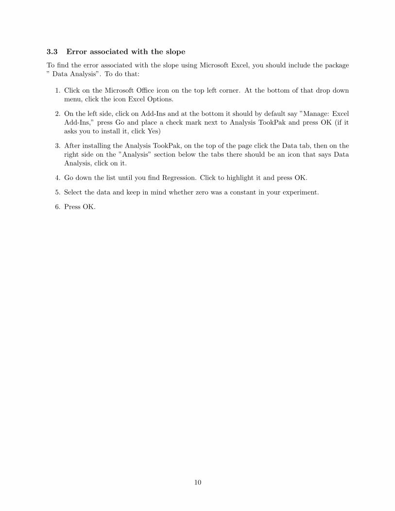
3.3 Error associated with the slope

To find the error associated with the slope using Microsoft Excel, you should include the package” Data Analysis”. To do that:

1. Click on the Microsoft Office icon on the top left corner. At the bottom of that drop downmenu, click the icon Excel Options.

2. On the left side, click on Add-Ins and at the bottom it should by default say ”Manage: ExcelAdd-Ins,” press Go and place a check mark next to Analysis TookPak and press OK (if itasks you to install it, click Yes)

3. After installing the Analysis TookPak, on the top of the page click the Data tab, then on theright side on the ”Analysis” section below the tabs there should be an icon that says DataAnalysis, click on it.

4. Go down the list until you find Regression. Click to highlight it and press OK.

5. Select the data and keep in mind whether zero was a constant in your experiment.

6. Press OK.

10

4 General Problems on the Calculation of the Uncertainties

4.1 Proper rounding and proper units

1. You measure the length x of an objects. Which of the following ways to report the result arecorrect?

(a) x = (5.232± 0.001)

(b) x = (5.2± 0.001) mm

(c) x = (5.232± 0.001) mm

(d) x = (5.232± 0.1) mm

(e) x = (5± 1) mm

4.2 Propagation of errors

2. The two quantities x and y have an uncertainty x and y. Calculate the error in the followingcases:

(a) x− 2yAnswer: δx+ 2δy

(b) 4x− 5y

(c) 3xy

Answer: 3xy(δxx + δy

y

)(d) x3

y5

Answer: x3

y5

(3 δxx + 5 δyy

)(e)√x

Answer: 12

√x(δxx

)(f)√x3

(g)√

2xy

(h) 2√

x3y

Answer:√

x3y

(δxx + δy

y

)

(i) 2√

x3

3y

11

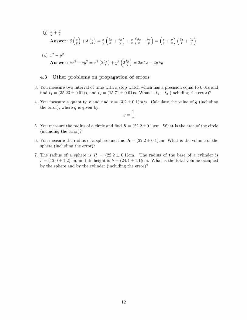
(j) xy + y

x

Answer: δ(xy

)+ δ

( yx

)= x

y

(δxx + δy

y

)+ y

x

(δxx + δy

y

)=(xy + y

x

)(δxx + δy

y

)(k) x2 + y2

Answer: δx2 + δy2 = x2(2 δxx)

+ y2(

2 δyy)

= 2x δx+ 2y δy

4.3 Other problems on propagation of errors

3. You measure two interval of time with a stop watch which has a precision equal to 0.01s andfind t1 = (35.23± 0.01)s, and t2 = (15.71± 0.01)s. What is t1 − t2 (including the error)?

4. You measure a quantity x and find x = (3.2 ± 0.1)m/s. Calculate the value of q (includingthe error), where q is given by:

q =1x

5. You measure the radius of a circle and find R = (22.2±0.1)cm. What is the area of the circle(including the error)?

6. You measure the radius of a sphere and find R = (22.2± 0.1)cm. What is the volume of thesphere (including the error)?

7. The radius of a sphere is R = (22.2 ± 0.1)cm. The radius of the base of a cylinder isr = (12.0± 1.2)cm, and its height is h = (24.4± 1.1)cm. What is the total volume occupiedby the sphere and by the cylinder (including the error)?

12

5 Problems On Graphing

1. (Points: 5) The data shown in the figure below were taken in an experiment which measuredthe velocity of an object. Draw the best fitting line by eye (without using the LSA formula)and write the corresponding velocity of the object. Use SI units for the velocity.

time @sD

posi

tion

@cmD

1.5 2.0 2.5 3.0 3.5

4.0

4.2

4.4

4.6

4.8

5.0

Answer v = −0.005 m/s

2. In an experiment to find the acceleration due to gravity, g, you measure the position (incm) of a free falling object at several different times (in seconds). When you plot your data(position in cm on the y-axis and time in s on the x-axis) in excel (or graphical analysis), theprogram gives for the best fit curve

y = 422.12x2 + 5.92x+ 2.04 (5.1)

(a) What is your result for the ”acceleration due to gravity”, g? Use SI units for youranswer.

(b) Suppose that the coefficients in (6.5) have a 5% error. What is your result for the”acceleration due to gravity”, g including the error? Use SI units for your answer.

3. The force exert on a wire long L and with a current I by a magnetic field perpendicular tothe wire is |~F | = IL| ~B|. An experimental plot shows |~F | as a function of L. The plot is astraight line, with equation (in SI units)

y = (11± 1)× 10−5x+ (0.021± 0.028). (5.2)

The current in the wire is I = (16± 2)mA. Find | ~B|, including the error (the SI units for Bis tesla, T).

13

4. Suppose that the two variables p and q are connected in the following way:

p2 =3παq .

If you want to find α from an experiment, you need to make a linear plot using several valuesfor p and q, and then find α from the slope of that graph. Explain the way you would do it:

Plot ............ on the y-axis and ............ on the x-axis.

Find α as: ............

and the uncertainty in α as: ............

Solution: One possibility is to plot p2 on the y−axis and q on the x−axis. The result wouldbe a straight line with slope m = 3π/α and intercept b = 0. Therefore,

α =3πm, δα =

3πm

(δm

m

)= α

(δm

m

)(5.3)

5. The same problem as before, but with:

pq = −√

3α


Find α as:

and the uncertainty in α as: ............


p = −π√α

q


Find α as:

and the uncertainty in α as:

7. Suppose that the two variables p and q are connected in the following way:

p2 =3παq +

32πh2

.

If you want to find α and h from an experiment, you need to make a linear plot using severalvalues for p and q, and then find α from the slope of that graph. Explain the way you woulddo it:


14

Find α as: ............ and the uncertainty in α as: ............

Find h as: ............ and the uncertainty in h as: ............

Solution: If you plot p2 on the y−axis and q on the x−axis, the result would be a straightline with slope m = 3π/α and intercept b = 3/(2πh2). Therefore,

α =3πm, δα =

3πm

(δm

m

)= α

(δm

m

)(5.4)

and

h =

√3

2πb, δh =

√3

2πb

(12δb

b

)= h

(12δb

b

)(5.5)


pq =√

2πα+ hq





p =

√3α2

q+ 2h3




15

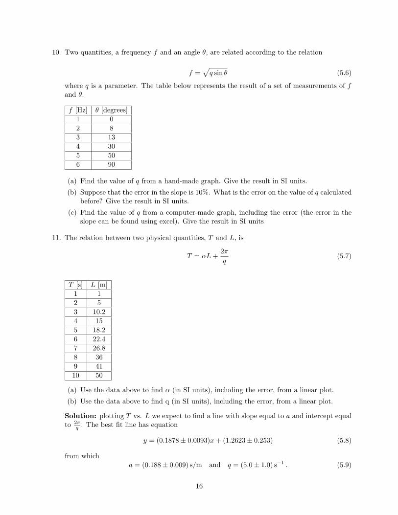
10. Two quantities, a frequency f and an angle θ, are related according to the relation

f =√q sin θ (5.6)

where q is a parameter. The table below represents the result of a set of measurements of fand θ.

f [Hz] θ [degrees]1 02 83 134 305 506 90

(a) Find the value of q from a hand-made graph. Give the result in SI units.

(b) Suppose that the error in the slope is 10%. What is the error on the value of q calculatedbefore? Give the result in SI units.

(c) Find the value of q from a computer-made graph, including the error (the error in theslope can be found using excel). Give the result in SI units

11. The relation between two physical quantities, T and L, is

T = αL+2πq

(5.7)

T [s] L [m]1 12 53 10.24 155 18.26 22.47 26.88 369 4110 50

(a) Use the data above to find α (in SI units), including the error, from a linear plot.

(b) Use the data above to find q (in SI units), including the error, from a linear plot.

Solution: plotting T vs. L we expect to find a line with slope equal to a and intercept equalto 2π

q . The best fit line has equation

y = (0.1878± 0.0093)x+ (1.2623± 0.253) (5.8)

from whicha = (0.188± 0.009) s/m and q = (5.0± 1.0) s−1 . (5.9)

16

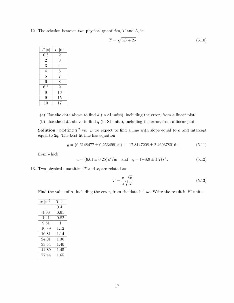
12. The relation between two physical quantities, T and L, is

T =√aL+ 2q (5.10)

T [s] L [m]0.5 22 33 44 65 76 8

6.5 98 139 1510 17

(a) Use the data above to find a (in SI units), including the error, from a linear plot.

(b) Use the data above to find q (in SI units), including the error, from a linear plot.

Solution: plotting T 2 vs. L we expect to find a line with slope equal to a and interceptequal to 2q. The best fit line has equation

y = (6.6148477± 0.253499)x+ (−17.8147208± 2.460378016) (5.11)

from whicha = (6.61± 0.25) s2/m and q = (−8.9± 1.2) s2 . (5.12)

13. Two physical quantities, T and x, are related as

T =π

α

√x

2(5.13)

Find the value of α, including the error, from the data below. Write the result in SI units.

x [m2] T [s]1 0.41

1.96 0.614.41 0.829.61 110.89 1.1216.81 1.1424.01 1.3033.64 1.4044.89 1.4577.44 1.65

17

14. Suppose that the relation in the problem above were

T =π

α

√x+ c

2(5.14)

Find α and c, including the error, from the data above.

Solution: If you square the expression you find

T 2 =(π2

2α2

)x+

(π2c

2α2

). (5.15)

This means that if we plot T 2 on the y−axis and x on the x−axis, we find a straight linewith slope m =

(π2

2α2

)and intercept b =

(π2c2α2

). Therefore,

α =

√π2

2m, δα = α

(12δm

m

)(5.16)

c =2α2 b

π2, δc = c

(2δα

α+δb

b

).

Excel gives the equation of the line:

y = (0.031443462± 0.004236863)x+ (0.617751± 0.135566) . (5.17)

Therefore,

α = (12.5± 0.8) m/s (5.18)c = (19.7± 7.0) m2 .

18

6 Problems on Basic Kinematics and Dynamics

6.1 Kinematics

1. I measure the velocity of an object which travels at constant speed along a straight line. Theinitial position of the object is (0.0 ± 0.1) cm, and the final position (100.0 ± 0.1) cm. Thetime taken to travel that distance is t = (37±1) s. Write the velocity of the object, includingthe error, in SI units.

Answer: d = 100cm, ∆d = 0.2 cm, t = 37s, ∆t = 1s, v = 2.7027 cm/s, δv/v = 0.028027,δv = 0.0757487 ' 0.08 cm/s, and so v = (2.70 ± 0.08) cm, which in SI units is v = (2.70 ±0.08)× 10−2 m.

6.2 Acceleration due to gravity

2. You can find the acceleration due to gravity, g, by dropping a stone to the ground from someheight h, and measuring the time it takes to reach the ground. The relation between timeand distance is

h = 1/2gt2 (6.1)

Suppose that you drop the stone from 2.4 m, and it takes 0.8 s to reach the ground. Youruncertainty on the distance is 10 cm, and on the time is 0.1 s.

(a) What is your value for the acceleration due to gravity? (include the error)

(b) Are you compatible with the value g = 9.81 m/s2?

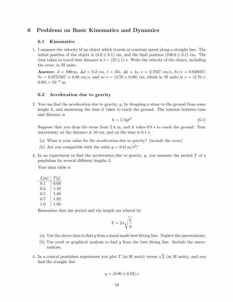
3. In an experiment to find the acceleration due to gravity, g, you measure the period T of apendulum for several different lengths L.

Your data table is

L[m] T [s]0.1 0.690.3 1.100.5 1.400.7 1.821.0 1.93

Remember that the period and the length are related by

T = 2π

√L

g

(a) Use the above data to find g from a hand-made best fitting line. Neglect the uncertainties.

(b) Use excel or graphical analysis to find g from the best fitting line. Include the uncer-tainties.

4. In a conical pendulum experiment you plot T (in SI units) versus√L (in SI units), and you

find the straight line

y = (0.90± 0.02)x

19

Your value for the ratio of the masses is µ = 0.21± 0.01.

Remember that:

T = 2π

√Lµ

g

Calculate g, including the error (in SI units).

Answer: g = (10.2± 0.9) m/s2.

6.3 Newton’s law

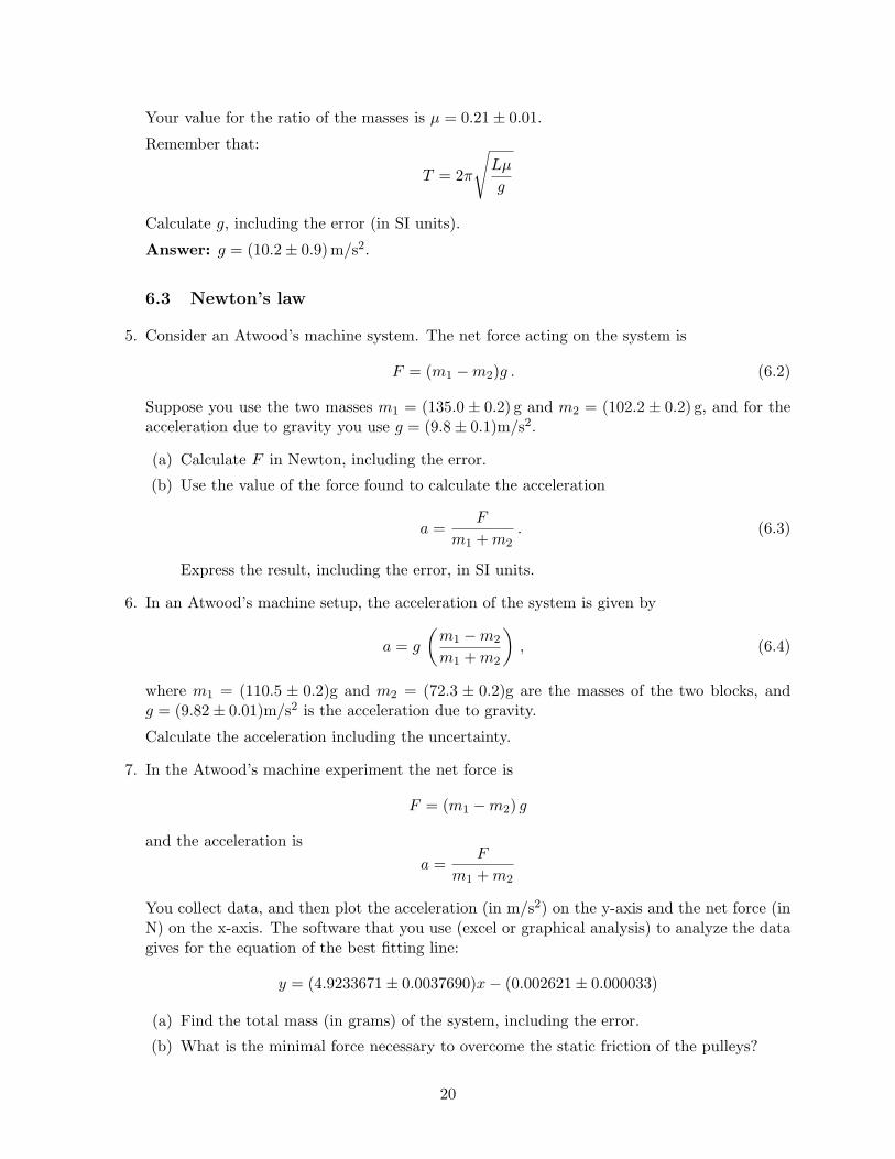
5. Consider an Atwood’s machine system. The net force acting on the system is

F = (m1 −m2)g . (6.2)

Suppose you use the two masses m1 = (135.0 ± 0.2) g and m2 = (102.2 ± 0.2) g, and for theacceleration due to gravity you use g = (9.8± 0.1)m/s2.

(a) Calculate F in Newton, including the error.

(b) Use the value of the force found to calculate the acceleration

a =F

m1 +m2. (6.3)

Express the result, including the error, in SI units.

6. In an Atwood’s machine setup, the acceleration of the system is given by

a = g

(m1 −m2

m1 +m2

), (6.4)

where m1 = (110.5 ± 0.2)g and m2 = (72.3 ± 0.2)g are the masses of the two blocks, andg = (9.82± 0.01)m/s2 is the acceleration due to gravity.

Calculate the acceleration including the uncertainty.

7. In the Atwood’s machine experiment the net force is

F = (m1 −m2) g

and the acceleration isa =

F

m1 +m2

You collect data, and then plot the acceleration (in m/s2) on the y-axis and the net force (inN) on the x-axis. The software that you use (excel or graphical analysis) to analyze the datagives for the equation of the best fitting line:

y = (4.9233671± 0.0037690)x− (0.002621± 0.000033)

(a) Find the total mass (in grams) of the system, including the error.

(b) What is the minimal force necessary to overcome the static friction of the pulleys?

20

6.4 Linear momentum

8. In an experiment to study the conservation of linear momentum, you collide two massesm1=38 g and m2=51 g . The uncertainty on the masses is negligible. The speeds of thecolliding particles are v1 = (3.1 ± 0.1) m/s and v2 = (2.4 ± 0.1) m/s. After the collision thetwo objects stick together and move with the speed vf = (2.8.± 0.2) m/s.

(a) Calculate the initial and final momentum, pi = m1v1+m2v2,and pf = (m1+m2)vf ,includingthe error.

(b) Is the momentum is conserved (pi = pf ) within the error?

9. In the ballistic pendulum experiment, you can find for the velocity of the bullet

v =

√gx2

2H

where H = (68.5 ± 0.1) cm is the height of the table, g = 9.81 is the acceleration due togravity (known with negligible error), and x = (284± 2) cm is the distance where the bulletlands, and for the velocity of the bullet+pendulum system

V =√

2gh

where h = (17± 1) cm. The mass of the pendulum is M = 148 g and the mass of the bulletis m = 50 g. The masses are known with negligible error.

(a) Calculate Pi = mv, including the error.

(b) Calculate Pf = (M +m)V , including the error.

(c) Is the momentum of the system conserved within the error?

6.5 Rigid bodies

10. In an experiment to study Newton’s laws applied to a rigid body, you apply the force F1 =(0.4± 0.05)N, to a body, with a lever arm d1 = (14.4± 0.2)cm, and a force F2 at a distanceR from the rotation center. You vary F2 and the angle θ between F2 and R. Equilibriumresults if

F1d1 = F2R sin θ (6.5)

If you plot F2 vs. (R sin θ)−1 (both in SI units) you find the curve

y = (0.07± 0.01)x+ (0.01± 0.005)

(a) Calculate the force F1 from the graph (including the error).

(b) Do you confirm the equation for static equilibrium (6.5) within the error?

11. Consider the static configuration of a cylinder of mass m = (120± 1)g, attached to a springwith constant k, and partially immersed in a fluid. The total force acting on the mass is

Ftot = mg − kx− ρgVsub = 0 (6.6)

where g = (9.80 ± 0.02)m/s2, ρ = (1075 ± 5)kg/m3, and Vsub is the volume of the cylinderimmersed in water.

21

To find k you measure the spring stretch from the equilibrium position, x, for different valuesof Vsub, and find the best fit to your data (in SI units)

y = (−2742± 2)x+ (0.32± 0.01)

(a) Calculate k ±∆k from the slope of the graph.

(b) Calculate k ±∆k from the intercept of the graph.

(c) Do the two values found agree within the error?

22

7 Problems on Waves and Sound

1. In an experiment to study standing waves, you use a string whose mass per length is µ =(1.8± 0.1)× 10−3kg/m. You look at the fundamental mode, whose frequency f is related tothe length L and tension T of the string by the following equation

L =1

2f

√T

µ. (7.1)

You make a plot with L on the y-axis and√T on the x-axis, and find that the best fitting

line isy = (8.3± 0.3)× 10−3 x+ (0.2± 0.4).

in SI units. What is the value of the frequency of the wave (including the error)? Expressyour result in SI units (Hz).

2. The temperature in a room is T = 19.8 degrees Celsius (the uncertainty in the tempera-ture is negligible). The relation that describes the dependence of the velocity of the soundwaves in air on the temperature is

v = v0 ×√

1 +T

273(7.2)

where v0 = (330 ± 2) m/s is the velocity of the sound in air (at zero Celsius) and T is thetemperature of the air in degrees Celsius.

(a) Calculate the velocity of the sound waves v, including the error. Express your result inSI units.

(b) More challenging question: Suppose now that the uncertainty in the temperature is∆T = 0.2 degrees Celsius. What would the uncertainty in the velocity be in this case?

3. In order to study the dependence of the velocity of the sound waves in air on the temperature,you collect data of the velocity at different temperatures. The relation that describes thisdependence is

v = v0 ×√

1 +T

T0(7.3)

If you plot v2 (in m2/s2) on the y−axis, and T (in C) on the x−axis, you find (from theleast-square-fit analysis) the relation

y = (398± 8)m2/(s2 C) + (108100± 1000)m2/s2 (7.4)

Calculate v0 and T0 including the errors.

23

8 Problems on Thermodynamics

1. A piece of metal with mass mm = (312±2) g, initial temperature Tm = (21±1) C, and specificheat cm = (128± 1) J/kgC, is brought into contact with water of mass mw = (1.472± 2) g,and initial temperature Tw = (88 ± 1) C. The specific heat of the water is cw = (4186 ± 1)J/kgC.

To find the equilibrium temperature Tf , (neglecting the heat exchange with the environment)you need to impose the equation

mmcm(Tf − Tm) +mwcw(Tf − Tw) = 0 . (8.1)

Calculate the equilibrium temperature (Tf ) of the water+metal system, including the error.

2. A piece of metal with mass mm = 308 g, initially at room temperature Tm = (21.0± 0.2) C,is brought into contact with water of mass mw = 192 g, and initial temperature Tw =(82± 0.8) C. The equilibrium temperature is Tf = (72± 1)C. The specific heat of the wateris cw = (4180± 10) J/kgC.

To find the specific heat of the metal, cm, you use the equation

mmcm(Tf − Tm) +mwcw(Tf − Tw) = 0 . (8.2)

Calculate the the specific heat of the metal, cm, including the error.

24

9 Problems on DC-Circuits

9.1 Ohm’s law

1. In a DC circuit, the electric current is I = (15.8 ± 0.1)µA, and the potential is V = (2.32 ±0.02)V. Find the resistance including the error. Write the result in SI units, and roundproperly (keep only one or two significant digits for the error, and round the result so thatits accuracy is the same as the accuracy of the error).

2. The figure below shows the current vs. potential graph for a resistor.

IAAE

VAVoltE1 2 3 4 5

0.05

0.10

0.15

0.20

(a) Find the resistance;Answer: Slope=(1/25)Ω−1 = 0.04Ω−1, so R = 25Ω.

(b) Suppose that the error in the slope s of the graph is δs = 1.17647× 10−3Ω−1. Calculatethe error δR in the resistance.Answer: δs/s = δR/R, so δR/R = 0.0294118.So δR = R× 0.0294118 = 0.735294Ω ' 0.7Ω.

(c) Write the result for the resistance (including the error ) properly rounded.Answer: R = (25.0± 0.7)Ω

3. The best fit line for a current vs. potential graph for a resistor has equation (we are using SIunits)

I = (3.08± 0.02)× 10−3 V + (0.002± 0.004)

(a) Find the resistance.

(b) Calculate the error δR in the resistance.

(c) Write the result for the resistance (including the error ) properly rounded.

25

9.2 Diodes

4. A diode is connected in reverse bias to a 1.5 V battery. What is (approximately) the currentthat you expect it would flow through it?

5. Draw the Current versus Voltage characteristic (CVVC) of the semiconductor diode

6. Consider the circuit below

(a) Do you expect a linear relation between the voltage and the current in the circuit?Explain.

(b) Indicate the p and n part of the diode in the figure

(c) Is the p-n junction in forward or reverse bias?

(d) What is the current that you expect to measure in this configuration (positive, negative,zero, directly proportional to the potential, inversely proportional to the potential)?

7. Consider the circuit below

(a) Do you expect a linear relation between the voltage and the current in the circuit?

(b) Indicate the p and n part of the diode in the figure

(c) Is the p-n junction in forward or reverse bias?

(d) What is the current that you expect to measure in this configuration (zero, directly pro-portional to the potential, inversely proportional to the potential, exponentially relatedto the potential, logarithmically relater to the potential)?

26

9.3 Parallel and series of resistors and Kirchhoff’s rules

8. Find the formula for equivalent resistance and its uncertainty for the circuits shown below

9. Find the equivalent resistance (including the error) of the circuit shown below

10. Find the equivalent resistance (including the error) of the circuit shown below

27

11. Consider the circuit in figure 1. The values of the resistances are R1 = (22.6 ± 0.2) × 103Ω,R2 = (8.6± 0.1)× 103Ω, R3 = (9.0± 0.1)× 103Ω.

Figure 1: Figure of circuit for problems 11 and 12

(a) Draw the equivalent circuit (with just one resistor, Req);

(b) Calculate R12, including the error. Write R12 ± δR12 properly rounded.

(c) Calculate Req, including the error. Write Req ± δReq properly rounded.

(d) Suppose that ∆V = (2.00± 0.02)V. Find the current I including the error.

12. Consider the circuit in figure 1. Circle the correct statements.

(a) The potential in A is the same as the potential in B.

(b) The potential difference between A and D is zero.

(c) The potential difference between C and D is ∆V .

(d) The potential difference between D and K is ∆V .

(e) The potential difference between A and K is ∆V .

(f) The current flowing through R1 is the same as the current flowing through R3.

13. Consider the circuit in the figure below with R1 = (15 ± 1.5)kΩ, R2 = (10 ± 1)kΩ, R3 =(50± 5)kΩ, V1 = (5.0± 0.1) V, V2 = (10.0± 0.1) V. The currents are known with negligibleuncertainties: I1 = 2.9× 10−4A, I2 = 7.1× 10−5A, I3 = 2.1× 10−4A.

Verify the Kirchhoff’s equations for loop 1 and loop 2, and specify if they are satisfied withinthe error. (Show the calculations)

28

14. Consider the circuit in the figure below with R1 = (15 ± 1.5)kΩ, R2 = (10 ± 1)kΩ, R3 =(50± 5)kΩ, V1 = (5.0± 0.1) V, V2 = (10.0± 0.1) V. The currents are known with negligibleuncertainties: I1 = 2.9× 10−4A, I2 = 7.1× 10−5A, I3 = 2.1× 10−4A.

Verify the Kirchhoff’s equations for loop 1 and loop 2, and specify if they are satisfied withinthe error. (Show the calculations)

9.4 RC-circuits

15. In a RC circuit the capacitor has capacitance C = (15± 1)µF, the resistance is R = (2500±200)Ω, and the potential of the battery is V = 15V.

(a) Find the time constant of the circuit (including the error).Solution: The time constant of a RC circuit, which means a circuit with a resistor anda capacitor (besides, of course, a generator), is

τ = RC . (9.1)

Notice that 1 Farad times 1 Ohm equals 1 second. In our case,

τ = 2500× 15× 10−6s

[1±

(225

+115

)]= (3.75± 0.55)× 10−2 s . (9.2)

(b) What is the charge on the capacitor after 100µs? (disregard the error).Hint: Remember that

Q(t) = CV(

1− e−t/τ)

(9.3)

(c) What is the current in the circuit after 100µs? (disregard the error).Hint: Remember that

I(t) =V

Re−t/τ (9.4)

16. In a RC circuit the capacitor has capacitance C = (1.5 ± 0.1)µF, the resistance is R =(1200± 200)Ω, and the potential of the battery is V = 11V.

(a) Find the time constant of the circuit (including the error).

(b) What is the charge on the capacitor after 20µs? (disregard the error).

(c) What is the current in the circuit after 20µs? (disregard the error).

(d) After how long is the current in the circuit 20% of the initial current? (disregard theerror).

29

(e) After how long is the charge on the capacitor 20% of the final charge? (disregard theerror).

17. In a RC circuit the capacitor has capacitance C = (11 ± 1)µF, and there are 2 resistors inseries with resistances R1 = (1500 ± 200)Ω and R2 = (500 ± 100)Ω. The potential of thebattery is V = (12± 1)V.

(a) Find the equivalent resistance of the circuit (including the error).Answer: Req = (2000± 300) Ω

(b) Find the time constant of the circuit (including the error).Answer: τ = ReqC = (2000× 11× 10−6)s = (2.2± 0.5)× 10−2s

(c) What is the initial current in the circuit (including the error).Answer: I = V

Req= (6.0± 1.4)× 10−3A

(d) What is the current in the circuit after 10−2s (disregard the error).Answer: 3.80842× 10−3A

18. During the charging process of a capacitor in a RC-circuit, the potential across the capacitorevolves as

Vc = V(

1− e−t/τ)

(9.5)

You collect data of the voltage across the capacitor at different times. Your best fit is

y = A(1− e−B t

)(9.6)

with A = (1.47± 0.001) in SI units, and B = (152± 2) in SI units.


(b) What is the meaning of the parameter A?

19. During the charging of a capacitor in a RC-circuit, the current in the circuit evolves as

I =V

Re−t/τ (9.7)

with V = 12 V (negligible uncertainty). You collect data of the current in the circuit atdifferent times, and plot ln I versus t. Your best fit is

y = A+Bx (9.8)

with A = −4.6 (negligible uncertainty), and B = −25.6± 0.1.


(b) Find the resistance R of the circuit (ignore the error)?

30

10 Problems on Resonant Circuits

1. What is the resonant frequency in an LRC circuit?

2. How does the resonant frequency in an LRC circuit change is the capacitance C is doubled?

3. How does the resonant frequency in an LRC circuit change is the resistance R is doubled?

4. What is the definition of the quality factor Q in an LRC circuit?

5. The value of the components in a LRC circuit is R = (11 ± 2) × 103 Ω, L = (10 ± 1) mH,C = (5± 1)µF. The maximal voltage of the generator is V = (10± 1) V.

(a) Calculate the resonant frequency, including the error.

(b) Calculate the maximal current in the circuit, including the error. (NOTE: The currentis maximal when the frequency is resonant. In this case Imax = Vmax/R, since the effectsof L and C cancel each other).

(c) Calculate the quality factor Q, including the error, using the formula

1Q

= R

√C

L(10.1)

31

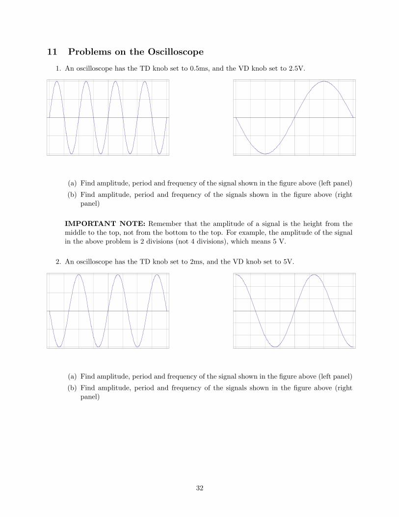
11 Problems on the Oscilloscope

1. An oscilloscope has the TD knob set to 0.5ms, and the VD knob set to 2.5V.

(a) Find amplitude, period and frequency of the signal shown in the figure above (left panel)

(b) Find amplitude, period and frequency of the signals shown in the figure above (rightpanel)

IMPORTANT NOTE: Remember that the amplitude of a signal is the height from themiddle to the top, not from the bottom to the top. For example, the amplitude of the signalin the above problem is 2 divisions (not 4 divisions), which means 5 V.

2. An oscilloscope has the TD knob set to 2ms, and the VD knob set to 5V.

(a) Find amplitude, period and frequency of the signal shown in the figure above (left panel)

(b) Find amplitude, period and frequency of the signals shown in the figure above (rightpanel)

32

12 Problems on Magnetic Field

1. What is the magnitude of the magnetic force exert on a straight wire with current I andlength L, if the magnetic field lines (of intensity B) form an angle θ with the wire?

2. The direction of the magnetic force is 1) parallel to the wire, 2) perpendicular to the wire or3) at an angle θ with respect to the wire?

3. What is the magnitude of the magnetic force exert on a straight wire with current I =(5 ± 0.5)A and length L = (5.0 ± 0.1)cm, immersed in a magnetic field of intensity B =(0.60 ± 0.03)T, if the magnetic field lines form an angle θ = π

6 with the wire? (ignore theerror in the angle).

4. The force exert on a wire long L and with a current I by a magnetic field perpendicular tothe wire is |~F | = IL| ~B|. An experimental plot shows |~F | as a function of L. The plot is astraight line, with slope s = (10± 1)× 10−5A·T. The current in the wire is I = (15± 1)mA.Find | ~B|, including the error (the SI units for B is tesla, T).

Answer:

B =s

I= 6.67× 10−3T (12.1)

δB = B

(δs

s+δI

I

)= 6.67× 10−3T × 0.1667 = 1.1× 10−3T (12.2)

33

13 Problems on Electromagnetic Waves and Optics

1. A beam of light strikes the boundary between two media (from medium-1 to medium-2) withan incident angle θi = 25. The angle of refraction is θt = 15. These angles are known withnegligible uncertainty. The first medium has a refractive index n1 = 1.2± 0.1. Calculate theindex of refraction of the second medium, including the error.

2. A beam of light strikes the interface between air and glass, and is refracted in the glass. Theangle of refraction θt is related to the incident angle θi by the Snell’s relation

nair sin θi = nglass sin θt , (13.1)

with nair = 1 (with negligible uncertainty). You plot sin θt (on the y-axis), vs. sin θi (on thex-axis), and find that the best fit line has equation

y = (7.23± 0.05)× 10−1x+ (0.022± 0.024). (13.2)

Calculate the index of refraction of the glass, including the error.

Answer: nglass = (1.38± 0.01).

3. A convex lens has a focal length of 5.0 cm. A concave lens has a focal length of -15.0 cm. A1cm high object is placed 25.0 cm to the left of the convex lens. The concave lens is placed10.0 cm to the right of the convex lens.

A) How far is the image from the object?

B) How high is the image?

C) Is the image upright or inverted?

Solution: It is recommended that you make a drawing.

From the problem, do1=25cm, so the primary image is located at

di1 =(

1f1− 1do1

)−1

=254

cm = 6.25 cm (13.3)

from the first lens. Since this value is positive, the image is to the right of the first lens.

The magnification of the primary image is

m1 = − di1do1

= −14. (13.4)

The primary image is the object for lens 2. From your drawing and the data, you can seethat it has to be located 3.75 cm to the left of lens 2. Therefore, do2=3.75 cm. So the imagefrom lens 2 is located at

di2 =(

1f2− 1do2

)−1

= −3 cm (13.5)

Since this value is negative, the image is to the left of the second lens.

Therefore, the distance of the final image to the object is 25cm+10cm-3cm=32cm.

The magnification of the secondary (final) image, with respect to the primary one, is

m2 = − di2do2

=45. (13.6)

34

So, the total magnification is

m1m2 = −15. (13.7)

Notice that this is negative, so the image is inverted.

Finally, the height of the image is

hi = −15ho = −2 mm . (13.8)

4. The intensity of light from a light bulb is related to the distance from the source accordingto the relation

I =P

4π R2(13.9)

You want to measure the power from a plot of the intensity (I) versus the inverse distancesquared R−2. Your best fit lines is

y = (36± 2)x+ (0.23± 0.65) (13.10)

in SI units (remember that the SI units for power is W). What is the power of the bulb (inWatts), including the error?

5. A monochromatic beam of light of wavelength 600 nm is incident normally on a diffractiongrating with a slit spacing of 1.70× 10−4 cm. What is the angle for the first order maximum(above the central bright fringe)?

6. A monochromatic beam of light of wavelength 533 nm is incident normally on a diffractiongrating with a slit spacing of 1.20× 10−4 cm. What is the angle for the first order maximum(above the central bright fringe)?

35

Review of Error Analysis and Practice Problems for PHY 201L/211L

Documents

Transcript of Review of Error Analysis and Practice Problems for PHY 201L/211L