Review of Discrete-Time System - ece.umd.edu · We use the subscript \a" to denote continuous-time...

$: Review of Discrete-Time System - ece.umd.edu · We use the subscript \a" to denote continuous-time (analog) signal and drop the subscript if the context is clear. The Fourier Transform$
Review of Discrete-Time System

Electrical & Computer EngineeringUniversity of Maryland, College Park

Acknowledgment: ENEE630 slides were based on class notes developed byProfs. K.J. Ray Liu and Min Wu. The LaTeX slides were made by Prof. Min Wu andMr. Wei-Hong Chuang.

Contact: [email protected]. Updated: August 28, 2012.

(UMD) ENEE630 Lecture Part-0 DSP Review 1 / 22

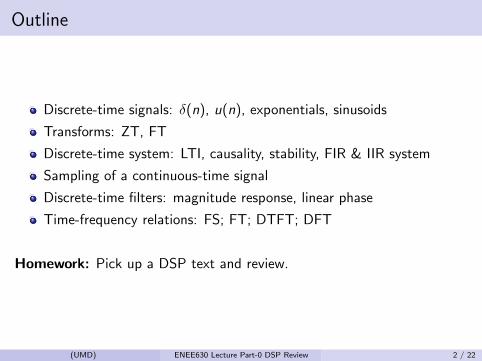
Outline

Discrete-time signals: δ(n), u(n), exponentials, sinusoids

Transforms: ZT, FT

Discrete-time system: LTI, causality, stability, FIR & IIR system

Sampling of a continuous-time signal

Discrete-time filters: magnitude response, linear phase

Time-frequency relations: FS; FT; DTFT; DFT

Homework: Pick up a DSP text and review.


§0.1 Basic Discrete-Time Signals

1 unit pulse (unit sample)

δ[n] =

1 n = 0

0 otherwise

2 unit step

u[n] =

1 n ≥ 0

0 otherwise

Questions:

What is the relation between δ[n] and u[n]?

How to express any x [n] using unit pulses?x [n] =

∑∞k=−∞ x [k]δ[n − k]


§0.1 Basic Discrete-Time Signals

3 Sinusoids and complex exponentials

x1[n] = A cos(ω0n + θ)x2[n] = ae jω0n

x2[n] has real and imaginary parts;known as a single-frequency signal.

4 Exponentials

x [n] = anu[n] (0 < a < 1) x [n] = anu[−n] x [n] = a−nu[−n]

Questions:Is x1[n] a single-frequency signal? Are x1[n] and x2[n] periodic?


§0.2 (1) Z-Transform

The Z-transform of a sequence x [n] is defined as

X(z) =∑∞

n=−∞ x [n]z−n.

In general, the region of convergence (ROC) takes the form ofR1 < |z | < R2.

E.g.: x [n] = anu[n]: X(z) = 11−az−1 , ROC is |z | > |a|.

The same X(z) with a different ROC |z | < |a| will be the ZT of a differentx [n] = −anu[−n − 1].


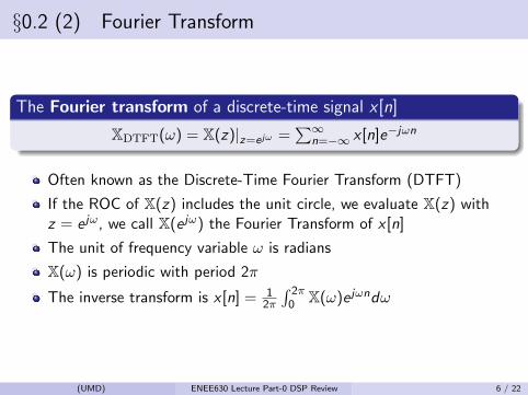
§0.2 (2) Fourier Transform

The Fourier transform of a discrete-time signal x [n]

XDTFT(ω) = X(z)|z=e jω =∑∞

n=−∞ x [n]e−jωn

Often known as the Discrete-Time Fourier Transform (DTFT)

If the ROC of X(z) includes the unit circle, we evaluate X(z) withz = e jω, we call X(e jω) the Fourier Transform of x [n]

The unit of frequency variable ω is radians

X(ω) is periodic with period 2π

The inverse transform is x [n] = 12π

∫ 2π0 X(ω)e jωndω



Question: What is the FT of a single-frequency signal e jω0n?

Since the ZT of an does not converge anywhere except for a = 0, theFT for x [n] = e jω0n does not exist in the usual sense.

But we can unite its FT as 2πδa(ω − ω0) for ω in the range between0 < ω < 2π and periodically repeating, by using a Dirac deltafunction δa(·).


§0.2 (3) Parseval’s Relation

Let X(ω) and Y(ω) be the FT of x [n] and y [n], then∑∞n=−∞ x [n]y∗[n] = 1

2π

∫ 2π0 X(ω)Y∗(ω)dω.

i.e., the inner product is preserved (except a multiplicative factor):

< x [n], y [n] >=< X(ω),Y(ω) > · 12π

1 If x [n] = y [n], we have∑∞

n=−∞ |x [n]|2 = 12π

∫ 2π0 |X(ω)|2dω

2 Parseval’s Relation suggests that the energy of x [n] is conserved afterFT and provides us two ways to express the energy.

Question: Prove the Parseval’s Relation.(Hint: start with applying the definition of inverse DTFT for x [n] to LHS)


§0.3 (1) Discrete-Time Systems

Question 1: How to characterize a general system?

Ans: by its input-output response (which may require us to enumerate allpossible inputs, and observe and record the corresponding outputs)

Question 2: Why are we interested in LTI systems?

Ans: They can be completely characterized by just one response - theresponse to impulse input


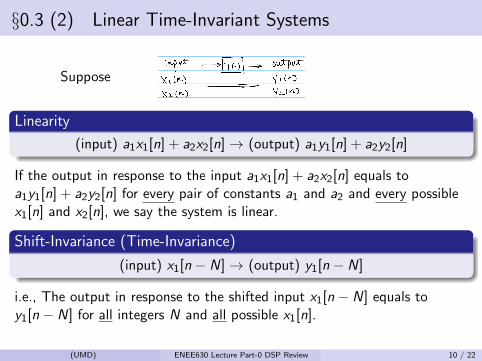
§0.3 (2) Linear Time-Invariant Systems

Suppose

Linearity

(input) a1x1[n] + a2x2[n]→ (output) a1y1[n] + a2y2[n]

If the output in response to the input a1x1[n] + a2x2[n] equals toa1y1[n] + a2y2[n] for every pair of constants a1 and a2 and every possiblex1[n] and x2[n], we say the system is linear.

Shift-Invariance (Time-Invariance)

(input) x1[n − N]→ (output) y1[n − N]

i.e., The output in response to the shifted input x1[n − N] equals toy1[n − N] for all integers N and all possible x1[n].


§0.3 (3) Impulse Response of LTI Systems

An LTI system is both linear and shift-invariant. Such a system can becompletely characterized by its impulse response h[n]:

(input) δ[n]→ (output) h[n]

Recall all x [n] can be represented as x [n] =∑∞

m=−∞ x [m]δ[n −m]⇒ By LTI property:

y [n] =∑∞

m=−∞ x [m]h[n −m]


§0.3 (4) Input-Output Relation of LTI Systems

The input-output relation of an LTI system is given by a convolutionsummation:

y [n]︸︷︷︸output

= h[n] ∗ x [n]︸︷︷︸input

=∑∞

m=−∞ x [m]h[n −m] =∑∞

m=−∞ h[m]x [n −m]

The transfer-domain representation is Y(z) = H(z)X(z), where

H(z) =Y(z)

X(z)=

∞∑n=−∞

h[n]z−n

is called the transfer function of the LTI system.


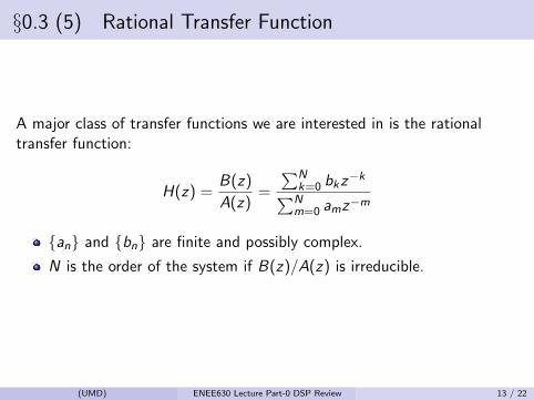
§0.3 (5) Rational Transfer Function

A major class of transfer functions we are interested in is the rationaltransfer function:

H(z) =B(z)

A(z)=

∑Nk=0 bkz

−k∑Nm=0 amz

−m

an and bn are finite and possibly complex.

N is the order of the system if B(z)/A(z) is irreducible.


§0.3 (6) Causality

The output doesn’t depend on future values of the input sequence.(important for processing a data stream in real-time with low delay)

An LTI system is causal iff h[n] = 0 ∀ n < 0.

Question: What property does H(z) have for a causal system?

Pitfalls: note the spelling of words “casual” vs. “causal”.


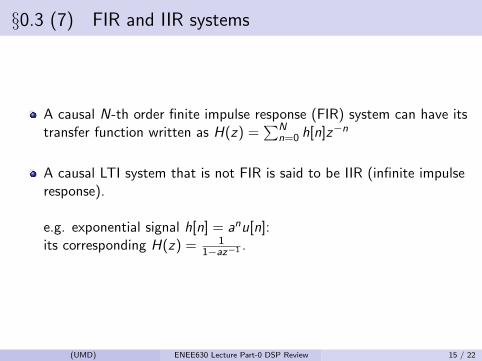
§0.3 (7) FIR and IIR systems

A causal N-th order finite impulse response (FIR) system can have itstransfer function written as H(z) =

∑Nn=0 h[n]z−n

A causal LTI system that is not FIR is said to be IIR (infinite impulseresponse).

e.g. exponential signal h[n] = anu[n]:its corresponding H(z) = 1

1−az−1 .


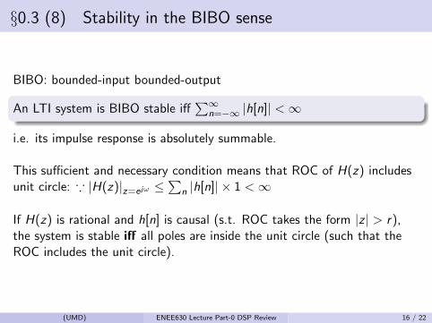
§0.3 (8) Stability in the BIBO sense

BIBO: bounded-input bounded-output

An LTI system is BIBO stable iff∑∞

n=−∞ |h[n]| <∞

i.e. its impulse response is absolutely summable.

This sufficient and necessary condition means that ROC of H(z) includesunit circle: ∵ |H(z)|z=e jω ≤

∑n |h[n]| × 1 <∞

If H(z) is rational and h[n] is causal (s.t. ROC takes the form |z | > r),the system is stable iff all poles are inside the unit circle (such that theROC includes the unit circle).



We use the subscript “a” to denote continuous-time (analog) signal anddrop the subscript if the context is clear.

The Fourier Transform of a continuous-time signal xa(t)Xa(Ω) ,

∫∞−∞ xa(t)e−jΩtdt “projection”

xa(t) = 12π

∫∞−∞Xa(Ω)e jΩtdΩ “reconstruction”

Ω = 2πf and is in radian per second

f is in Hz (i.e., cycles per second)


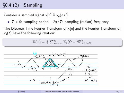
§0.4 (2) Sampling

Consider a sampled signal x [n] , xa(nT ).

T > 0: sampling period; 2π/T : sampling (radian) frequency

The Discrete Time Fourier Transform of x [n] and the Fourier Transform ofxa(t) have the following relation:

X(ω) = 1T

∑∞k=−∞Xa(Ω− 2πk

T )|Ω=ωT


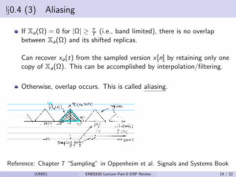
§0.4 (3) Aliasing

If Xa(Ω) = 0 for |Ω| ≥ πT (i.e., band limited), there is no overlap

between Xa(Ω) and its shifted replicas.

Can recover xa(t) from the sampled version x [n] by retaining only onecopy of Xa(Ω). This can be accomplished by interpolation/filtering.

Otherwise, overlap occurs. This is called aliasing.

Reference: Chapter 7 “Sampling” in Oppenheim et al. Signals and Systems Book


§0.4 (4) Sampling Theorem

Let xa(t) be a band-limited signal with Xa(Ω) = 0 for |Ω| ≥ σ, thenxa(t) is uniquely determined by its samples xa(nT ), n ∈ Z,

if the sampling frequency Ωs , 2π/T satisfies Ωs ≥ 2σ.

In the ω domain, 2π is the (normalized) sampling rate for anysampling period T .Thus the signal bandwidth can at most be π to avoid aliasing.


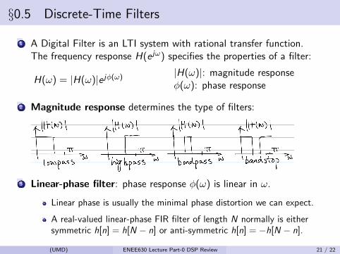
§0.5 Discrete-Time Filters

1 A Digital Filter is an LTI system with rational transfer function.The frequency response H(e jω) specifies the properties of a filter:

H(ω) = |H(ω)|e jφ(ω) |H(ω)|: magnitude responseφ(ω): phase response

2 Magnitude response determines the type of filters:

3 Linear-phase filter: phase response φ(ω) is linear in ω.

Linear phase is usually the minimal phase distortion we can expect.

A real-valued linear-phase FIR filter of length N normally is eithersymmetric h[n] = h[N − n] or anti-symmetric h[n] = −h[N − n].


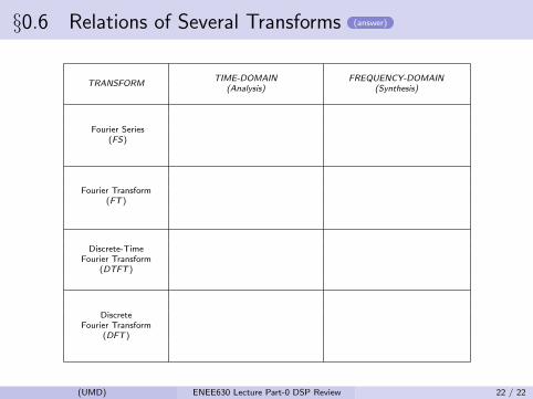
§0.6 Relations of Several Transforms (answer)

TRANSFORMTIME-DOMAIN FREQUENCY-DOMAIN

(Analysis) (Synthesis)

Fourier Series(FS)

x(t) continuous periodic Xn discrete aperiodic

Xn =1

T

∫ + T2

− T2

x(t)e−j2πnt/T dt x(t) =+∞∑

n=−∞Xne

j2πnt/T

Fourier Transform(FT )

x(t) continuous aperiodic X (Ω) continuous aperiodic

X (Ω) =

∫ +∞

−∞x(t)e−jΩtdt x(t) =

1

2π

∫ +∞

−∞X (Ω)ejΩtdΩ

(or in f where Ω = 2πf )

Discrete-TimeFourier Transform

(DTFT )

x[n] discrete aperiodic X (ω) continuous periodic

X (ω) =+∞∑

n=−∞x[n]e−jωn x[n] =

1

2π

∫ +π

−πX (ω)ejωndω

DiscreteFourier Transform

(DFT )

x[n] discrete periodic X [k] discrete periodic

X [k] =

N−1∑n=0

x[n]W knN x[n] =

1

N

N−1∑k=0

X [k]W−knN

(where W knN = e−j2πkn/N )


§0.6 Relations of Several Transforms

TRANSFORMTIME-DOMAIN FREQUENCY-DOMAIN

(Analysis) (Synthesis)

Fourier Series(FS)

x(t) continuous periodic Xn discrete aperiodic

Xn =1

T

∫ + T2

− T2

x(t)e−j2πnt/T dt x(t) =+∞∑

n=−∞Xne

j2πnt/T

Fourier Transform(FT )

x(t) continuous aperiodic X (Ω) continuous aperiodic

X (Ω) =

∫ +∞

−∞x(t)e−jΩtdt x(t) =

1

2π

∫ +∞

−∞X (Ω)ejΩtdΩ

(or in f where Ω = 2πf )

Discrete-TimeFourier Transform

(DTFT )

x[n] discrete aperiodic X (ω) continuous periodic

X (ω) =+∞∑

n=−∞x[n]e−jωn x[n] =

1

2π

∫ +π

−πX (ω)ejωndω

DiscreteFourier Transform

(DFT )

x[n] discrete periodic X [k] discrete periodic

X [k] =

N−1∑n=0

x[n]W knN x[n] =

1

N

N−1∑k=0

X [k]W−knN

(where W knN = e−j2πkn/N )


§0.3 (1) Discrete-Time Systems

Question 1: How to characterize a general system?

Ans: by its input-output response (which may require us to enumerate allpossible inputs, and observe and record the corresponding outputs)

Question 2: Why are we interested in LTI systems?

Ans: They can be completely characterized by just one response - theresponse to impulse input


Review of Discrete-Time System - ece.umd.edu · We use the subscript \a" to denote continuous-time...

Documents

Transcript of Review of Discrete-Time System - ece.umd.edu · We use the subscript \a" to denote continuous-time...