
Review of Aurora Energy 's maximum demand forecasting ... - Demand report.pdf · Review of Aurora...
86
Review of Aurora Energy 's maximum demand forecasting methodologies in its 2012 to 2017 regulatory proposal * Final report to the Australian Energy Regulator 3.0 9 September 2011
Transcript of Review of Aurora Energy 's maximum demand forecasting ... - Demand report.pdf · Review of Aurora...

Review of Aurora Energy 's maximum demand forecasting methodologies in its 2012 to 2017 regulatory proposal
*
Final report to the Australian Energy Regulator
3.0
9 September 2011

The SKM logo trade mark is a registered trade mark of Sinclair Knight Merz Pty Ltd.
Review of Aurora Energy 's maximum demand forecasting methodologies in its 2012 to 2017 regulatory proposal
FINAL REPORT TO THE AUSTRALIAN ENERGY REGULATOR
3.0
9 September 2011
SKM MMA ABN 37 001 024 095 Level 11, 452 Flinders Street, Melbourne 3000 PO Box 312, Flinders Lane Melbourne VIC 8009 Australia Tel: +61 3 8668 3000 Fax: +61 3 8668 3001 Web: www.SKM MMA.com
COPYRIGHT: The concepts and information contained in this document are the property of SKM MMA. Use or copying of this document in whole or in part without the written permission of Sinclair Knight Merz constitutes an infringement of copyright.
LIMITATION: This report has been prepared on behalf of and for the exclusive use of SKM MMA’s Client, and is subject to and issued in connection with the provisions of the agreement between Sinclair Knight Merz and its Client. Sinclair Knight Merz accepts no liability or responsibility whatsoever for or in respect of any use of or reliance upon this report by any third party.

Review of Aurora's maximum demand forecasts
SINCLAIR KNIGHT MERZ
Finall report to AER 9 September 2011 PAGE i
Contents
1. Executive Summary 1
1.1. Background 1
1.2. History and forecasts 1
1.3. Key drivers for the next regulatory period 2
1.4. Review of methodology at Terminal Station (TS) level 2 1.4.1. Weather correction 5
1.4.2. Coincidence factor adjustment 6
1.4.3. Reconciliation 6
1.5. Aurora methodology and forecasts at feeder level 7
1.6. Trend projection based on data from 2005 to 2011 8
2. Introduction 11
2.1. Aurora Energy’s Regulatory Proposal 11
2.2. Review of Aurora Energy’s Regulatory Proposal 11
2.3. Review of Aurora Energy’s demand forecasting methodologies 11
2.4. Spatial and global maximum demand forecasts 12
2.5. Process undertaken 13
2.6. Issues covered by this report 14
2.7. Assessment criteria 14
2.8. Conventions adopted 14
2.9. Forecasts assessed 16 2.9.1. 50 POE forecasts 16
2.9.2. Basis of the capex forecasts 16
2.10. Layout of the report 16
2.11. Handling potential conflicts of interest 17
3. History, forecasts and key drivers 18
3.1. Network winter MD 18
3.2. Non-coincident winter MD at terminal stations 19
3.3. Key drivers 20
3.4. Weather 20 3.4.1. Weather correction 20
3.4.2. Changing weather 22
3.5. Population and customer number growth 25
3.6. Economic growth 25
3.7. Government policies 27
3.8. Gas supply and reticulation 28
3.9. Price effects 28

Review of Aurora's maximum demand forecasts
SINCLAIR KNIGHT MERZ
Final report to AER 9 September 2011 PAGE ii
3.10. Summary of key drivers expected over the period 29
4. Aurora’s MD forecasting methodology at system, Terminal Station and Zone Substation levels 30
4.1. Overview 30
4.2. Basis of review 30
4.3. Review of Methodology Steps 34 4.3.1. Capturing Daily MD for each substation 34
4.3.2. Adjustments due to block loads, transfers, embedded generation - Steps 4 and 7 34
4.3.3. Trends and Base Forecast Steps 5 and 6 35
4.3.3.1. Growth Rates 35
4.3.3.2. Starting Point 35
4.3.4. Coincidence Factors step 8 36
4.3.5. Reconciliation to NIEIR steps 9 to 11 37
4.3.6. Conversion from MW to MVA in step 12 38
4.4. Summer peaking substations 39
4.5. Weather correction methodology and application 39 4.5.1. ACIL Weather Correction Methodology 39
4.5.1.1. ACIL 50 POE Historic MDs for Chapel St 40
4.5.1.2. ACIL 50 POE Historic MDs for Geilston 42
4.5.2. SKM MMA Approach to 50 POE weather correction 43
4.5.2.1. Basic 50 POE MD calculations 43
4.5.2.2. Basic plus “scatter” 43
4.5.2.3. Simulation approach to 50 POE MD 43
4.5.2.4. Results 44
4.5.3. Potential Issues noted from inspection of daily MD vs Temperature scatter plots46
4.5.3.1. Chapel St 2010 46
4.5.4. Chapel St 2009 46
4.5.5. Geilston Bay 2006 46
4.5.5.1. Geilston 2007 47
4.5.5.2. Conclusion on scatter charts 47
4.5.6. Impact of recommended changes on final forecasts 47
4.5.7. Conclusion for historic weather correction 48
4.6. Reconciliation to forecast derived from the NIEIR forecasts for Transend 50 4.6.1. Derivation of numbers from NIEIR report to Transend 51
4.6.2. Timeliness and relevance 52
4.6.3. Different assumed levels of key drivers 52
4.6.4. NIEIR methodology 53
4.6.5. Jump in the initial year 53
4.6.6. Conclusions on use of NIEIR forecasts for Aurora 55

Review of Aurora's maximum demand forecasts
SINCLAIR KNIGHT MERZ
Final report to AER 9 September 2011 PAGE iii
5. Aurora’s MD forecasting methodology at feeder level 56
5.1. RIN forecast methodology 56
5.2. Feeder forecast methodology used for capex in the Proposal 56
5.3. Review of feeder forecasts for Geilston Bay and Chapel Street 58 5.3.1. Some example feeders from Geilston Bay 60
5.3.2. Some example feeders from Chapel Street 64
5.3.3. Conclusions from the assessment of feeders in Chapel Street and Geilston Bay 67
5.4. Consideration at the TS and system levels 68
6. Conclusions and recommendations 71
6.1. Aurora methodology and forecasts at TS level 71 6.1.1. Approach and methodology 71
6.1.2. Weather correction 71
6.1.3. Coincidence factor adjustment 72
6.1.4. Reconciliation 72
6.2. Aurora methodology and forecasts at feeder level 73
6.3. Trend projection based on data from 2005 to 2011 74 6.3.1. A preliminary seven year trend projection for system MD reconciliation 75
7. Glossary 78

Review of Aurora's maximum demand forecasts
SINCLAIR KNIGHT MERZ
Final report to AER 9 September 2011 PAGE iv
Document history and status
Revision Date issued Reviewed by Approved by Date approved Revision type
1.0 1 August 2011 RL BT 1 August 2010 Draft to AER
2.1 9 September 2011 MP MG for BT 7 September 2011 Draft Final After comments from AER
3.0 26 September 2011 MG for BT Final
Printed: 26 September 2011
Last saved: 26 September 2011 11:15 AM
File name: I:\SHIN\Projects\SH43078\Deliverables\Reports\SH43078 Final MD report 26 September 2011.docx
Author: Michael Goldman
Project manager: Michael Goldman
Name of organisation: Australian Energy Regulator
Name of project: Review of Aurora's maximum demand and energy forecasts
Name of document: Review of Aurora's maximum demand forecasts
Document version: 3.0
Project number: SH43078

Review of Aurora's maximum demand forecasts
SINCLAIR KNIGHT MERZ
Final report to AER 9 September 2011 PAGE 1
1. Executive Summary
1.1. Background
Under the National Electricity Law, the Australian Energy Regulator (AER) is responsible for the
economic regulation of electricity distribution services provided by distribution network service
providers (DNSPs) in the National Electricity Market (NEM).
In accordance with these responsibilities, the AER is conducting an assessment into the appropriate
revenues and prices for the Aurora DNSP from 1 June 2012 to 30 June 2017. Forecasts of
maximum demand play a significant role in determining capital expenditure (capex) forecasts. The
AER has commissioned SKM MMA to assist it by reviewing the methods, inputs and data sources
used by Aurora in its demand forecasting. We have focused on the 50 POE winter forecasts as
being the most relevant for growth capex. We have examined the Chapel Street terminal station and
Geilston Bay zone substation, both around Hobart, in detail.
1.2. History and forecasts
Aurora’s history and forecasts at system level are illustrated in Figure 1-1 along with trend lines
based on the six year and most recent four year trends.
Figure 1-1 Network maximum demand, historical actual, weather corrected actual and forecast, MW

Review of Aurora's maximum demand forecasts
Final report to AER 9 September 2011 PAGE 2
Based on the graph, two key questions need answering: is the initial expected jump of about 12%
from 2010 actuals realistic and will growth history be more similar to that over the period 2005 to
2010 or over the period 2007 to 2010 or be intermediate between the two?
1.3. Key drivers for the next regulatory period
We have assessed a number of key drivers of maximum demand for the next regulatory period.
Based on this assessment, we would expect that the past three years of actuals would be weather
corrected upwards by some 20-30 MW as minimum winter temperatures have been unusually mild.
Beyond this impact, however, most of the key drivers we have considered, population and
household growth, economic growth, government policy effects and price impacts all suggest that
growth over the period 2011 to 2017 might be expected to be lower than it was over the period
2005 to 2010.
1.4. Review of methodology at Terminal Station (TS) level
We have reviewed the methodology as described and its application by ACIL Tasman, the
consultant to Aurora who prepared the MD model and/or Aurora. A summary of the methodology
with brief comments on both methodology and application is presented in Table 1-1.
Table 1-1 Summary of methodology and brief comments
Step ACIL Method Output SKM MMA comment on method
SKM MMA comment on application
0 Historic Daily MD
Select the daily MD for winter and summer.
Daily MD for each station
Ok as long as errors and temporary transfers are filtered.
1 Temperature Sensitivity
Determine the temperature sensitivity for each TS each year using the daily MD and local weather station. Excludes weekends
Temperature sensitivity MW/°C for each TS for each year
Choice of weather variable is important.
Ignores the quality of the temperature sensitivity regression fit
2 Standard Weather
ACIL selects the day of coldest average temperature from each winter, then calculates the 50th and 10th percentile. Includes non-workdays. As standard, ACIL also uses a long-term distribution, despite evidence that the past
10 and 50 POE temperature for each weather station based on long-term temperatures
Weekends should not be included in step 1 if it has been decided that the maximum demand does not occur on a weekend. The long-term averages are
ACIL is slightly overestimating the 10 and 50 POE weather by including weekends when calculating the standard weather and further by using a long-term average as the standard.

Review of Aurora's maximum demand forecasts
Final report to AER 9 September 2011 PAGE 3
Step ACIL Method Output SKM MMA comment on method
SKM MMA comment on application
10 and 20 years have seen significant warming.
unlikely to be appropriate given the difference of the past 20 years compared to the previous 20 years. SKM MMA recommends using a 20 year history.
3 50 POE MD Take the actual maximum demand recorded each winter and adjust by the difference between the actual temperature on the day of maximum demand and the 50 POE temperature (step 2) using the temperature sensitivity from step 1.
Temperature Corrected History
This approach will generally over-estimate the 50 POE MD.
Weather correction is likely to be overstated. Over the past 6 years ZSS MDs have been corrected up in 92% of cases. This is unlikely to be the case. In addition, the extent of weather correction at system level is significantly higher than the difference between ACIL’s 50 POE and 10 POE MD and also between NIEIR’s 50 POE and 90 POE MD.
4 Adjustments Adjust the temperature corrected MD history to undo the changes due to transfers, blocks, etc...
TC minus adjustment
Ok
5 Trend Determine trend or growth rate on the temperature corrected adjusted series.
Growth rate Ok Default option is the 6 year linear growth. Reasons have been provided where other rates are used.
6 Base Forecast Select trend measure for each TS. Calculate the forecast growth as if the adjustments had not occurred.
Start from weather corrected 2010 value rather than trend value.
This is in order to not have large unexplained movements in the initial year

Review of Aurora's maximum demand forecasts
Final report to AER 9 September 2011 PAGE 4
Step ACIL Method Output SKM MMA comment on method
SKM MMA comment on application
7 Re-adjust Reverse the adjustment process of step 4
Base plus adjustment forecast MDs by TS
Ok Used a threshold of 1 MW rather than 5% of TS size.
8 Coincidence factors
Divide the TS demand at time of system peak by TS Actual MD
Varies year to year.
See below
9 Coincident MD Forecast
Calculate coincident MD forecasts using the “Base plus adjustment” forecasts multiplied by the most recent years coincidence factor
Coincident MD forecast by TS
Ok ACIL Tasman has used only the most recent year’s (2010) coincidence factors which are lower than average. In forecasts we consider the average over a number of years should be used.
10 Reconcile to System Coincident forecast
Sum of coincident forecast MDs against NIEIR forecast of Aurora system MD
Reconciled Coincident Forecasts by TS Reconciliation factor for each forecast year.
Ok We have concerns about the use of forecasts which have not been validated as suitable for the purpose, use different key drivers and assume a very significant increase in year one. Aurora relies very heavily on system reconciliation to correct for any other methodological issues such as weather correction.
11 Non-coincident reconciled MD
Divide the reconciled coincident forecast by the coincidence factor used in step 9.
Reconciled Non-coincident MD
Ok We consider that forecasts need to use the average coincidence factor over a number of years, not that from the most recent year. Using a lower coincidence factor than average will inflate non-coincident forecasts.

Review of Aurora's maximum demand forecasts
Final report to AER 9 September 2011 PAGE 5
Step ACIL Method Output SKM MMA comment on method
SKM MMA comment on application
12 Non-coincident reconciled MVA
Convert MD to MVA using power factor
Reconciled Non-coincident MVA for each TS
Ok Have used the PF from the most recent year.
While the approach and methodology used by Aurora in deriving its forecasts at TS level is
generally considered to be good practice in outline, we have three significant concerns about its
application. These are in the steps related to weather correction, coincidence factor adjustments
and reconciliation.
1.4.1. Weather correction
We believe that the method used by ACIL Tasman to weather correct to 50 POE will overstate the
actual weather corrected amounts by a material amount. This is because:
ACIL Tasman has included weekend as well as weekdays in its analysis, despite stating its
expectation that peak demand will occur on weekdays.
The 50 POE temperatures assessed have been based on long-term weather time series.
Because of the warming that has taken place in Tasmania over recent years we consider that
using the average temperature over the past 20 years is more appropriate.
The method used by ACIL Tasman to derive the 50 POE MD from the temperature on the day
of actual peak demand is likely to produce an inflated weather correction when compared to a
combination of regression and simulation. This is evidenced by ACIL Tasman weather
correcting system MD up by about 60 MW over each of the past three years, while the
difference between a 50 POE and 90 POE is only of the order of 30 MW or less according to
both SKM MMA .
We have assessed the degree of over-statement of weather correction to be some 4% to 8% in
the two TS we have reviewed in detail. The method used to derive the 50 POE MD from the
day of annual maximum demand is the largest contributor to this over-statement.
ACIL Tasman has argued that, even if its weather correction is over-stated, this would largely be
overcome by the reconciliation process. While we largely agree with this argument, the over-
statement of weather correction in this case results in an understatement of the amount of
reconciliation that needs to take place. This is especially important when there are uncertainties
about the reconciliation itself (see below).
While we have concerns about the methodology used to weather correct, we do not consider that
the methodology introduces any obvious bias into relative TS growth rates.

Review of Aurora's maximum demand forecasts
Final report to AER 9 September 2011 PAGE 6
1.4.2. Coincidence factor adjustment
ACIL Tasman has converted to and from the sum of non-coincident TS historical and forecasts by
using the 2010 coincidence factor. However, this year had an atypically low coincidence factor,
possibly because it was a very mild winter. We consider it more appropriate to have used the
average of the past three to five years as initially proposed by ACIL Tasman. We recommend
using the average of the past five years.
This makes a material difference to the outcomes for non-coincident TS as these are calculated by
taking external system coincident forecasts and dividing by the coincidence factors. We have
estimated the difference to be some 2.5% in each year of the next regulatory period. As a result,
we consider that the Aurora non-coincident forecasts are inflated by at least this amount in each
year.
1.4.3. Reconciliation
The ACIL Tasman spatial forecasts built from bottom up at TS level are reconciled by Aurora to a
set of externally generated top down global system forecasts which have been derived by Transend
from Tasmania-wide forecasts generated by NIEIR.
The intention of a reconciliation of global and spatial forecasts is to ensure that the “macro”
drivers, economic and policy driven, at global level are filtered onto the more mechanistically
derived spatial forecasts. Typically the weather corrected spatial MD forecasts are diversified and
aggregated and then reconciled to the system MD forecasts by scaling up or down.
Aurora has taken the forecasts provided by Transend and used these numbers as the system MD
numbers. As a result, the spatial forecasts derived by ACIL Tasman have been scaled up by from
1.86%-3.39% each year in order to reconcile with these system forecasts. However, due to the
weather correction issues mentioned above, we believe that these factors materially understate the
extent of scaling required from 50 POE weather corrected historical and forecasts. For example,
the jump to the forecast 2011 of 1152 MW from the 2010 actual of 1022 MW plus an additional
(say) 30 MW of weather correction is very significant, some 100 MW or 9.5%. The rationale for
such a substantial increase due to the reconciliation process must be understood.
Although we consider that a reconciliation between bottom up spatial forecasts and top down
global forecasts generally represents good practice, we have a number of concerns about the
reconciliation process undertaken by Aurora to forecasts derived from NIEIR including:
The histories have not been fully reconciled to ensure that what is being forecast is consistent
with the Aurora system MD. Indeed, Aurora was not aware of the actual methodology used by
NIEIR. In other words, the NIEIR forecasts have not been validated for Aurora.
The growth drivers assumed by NIEIR are materially different to those assumed by Aurora.

Review of Aurora's maximum demand forecasts
Final report to AER 9 September 2011 PAGE 7
The translation of NIEIR forecasts for Aurora in 2010 and 2011 shows a significant jump in
the first year followed by years of moderate growth. Such a jump did not take place in 2010
and, based on evidence to date, is not expected to take place in 2011.
As a result we consider it likely that the system forecasts derived for Aurora are likely to be
over-stated in the first year and probably to 2017.
1.5. Aurora methodology and forecasts at feeder level
We understand that a significant proportion of the growth capex proposed for the next regulatory
period relates to high voltage feeders. As a result we have reviewed the growth forecasts at feeder
level at one TS and one ZSS. We understand that the capex programs were derived based on 2009
feeder actual MDs which had been grown at rates from the 2008 UES report. Further, we
understand that these programs were then re-assessed after the UES 2009 and the ACIL Tasman
2010 growth rates became available and were considered to still be applicable.
While we cannot comment on the capex programs, we have assessed that the use of the ACIL
Tasman instead of UES 2008 growth rates would have resulted in materially different growth for
many of the TS including for the Chapel Street and Geilston Bay substations. By comparing
forecast outcomes under both the UES 2008 and ACIL Tasman 2010 forecasts we have assessed
that, by 2017, out of the 42 TS assessed, the two MD forecasts are within ±5% of each other for
only 9 TS. Seventeen TS have UES forecasts more than 5% higher than ACIL forecasts (including
the Chapel Street TS and Lindisfarne TS which relates to Geilston Bay) while 16 have UES
forecasts more than 5% lower than ACIL forecasts. Clearly there are significant differences at a
number of TS which may feed into significant differences in feeder forecasts.
At the system level, however, the forecasts produced by using the 2009 actual starting values and
UES growth rates results, by 2017, in a value which is not materially different to the result of the
ACIL Tasman growth forecasts (1331 MW versus 1328 MW) for the sum of the non-coincident
connection points. Overall, the forecast growth rate between 2009 and 2017 is 2.0% pa for both the
UES 2008 and the ACIL Tasman reconciled methodology.
However, we have concluded above that the coincidence factors used by ACIL Tasman in its
forecasts are too low and that these should be changed to the average over the past 3 or 5 years.
Doing this would be expected to result in a reduction of the sum of the non-coincident MDs by
about 2.5%.in each year.
As a result, this would reduce the ACIL Tasman forecasts in each year and to 1295 MW in 2017
and an annual growth rate of 1.7% pa between 2009 and 2017. This is materially different to the
overall UES 2008 growth rate of 2% pa.

Review of Aurora's maximum demand forecasts
Final report to AER 9 September 2011 PAGE 8
This amended ACIL Tasman growth rate, combined with the different starting points from feeder
MDs in 2010 as listed in the RIN may result in a different feeder work program at some stations.
We recommend that Aurora be asked to provide feeder forecasts based on the RIN 2010
starting point growing at the ACIL Tasman growth rates amended to take into account a
diversity factor averaged over the past five years.
Even this result may be higher than would be expected to be the case if the global reconciliation
process, about which we have expressed concerns, is considered to be too high, especially in the
first year.
1.6. Trend projection based on data from 2005 to 2011
The actual system MD for winter 2010 and initial MD results to date for the network in winter
2011 (less than 1000 MW) suggest strongly that the forecast of a coincident system MD of 1152
MW in winter 2011 is unlikely to eventuate. This is likely to be due to a combination of the initial
jump in 2011 forecast based on reconciliation with the NIEIR forecast for Transend being too
steep, and the economic growth factors assumed by NIEIR under those forecasts and its forecasts
for Transend in 2011 being materially higher than those expected by ACIL Tasman. The
difference between forecast and recent actual MDs are illustrated in Figure 1-2.
If it is confirmed over the entire winter 2011 (that is by end August 2011) that the forecasts are
indeed significantly too high in the starting year, then we recommend that Aurora be asked to
reconcile to a forecast based on a trend growth line over the period 2005 to 2011. Such a
projection is provided as the solid purple line in Figure 1-2 below and compared with the ACIL
Tasman and NIEIR 2011 forecasts.

Review of Aurora's maximum demand forecasts
Final report to AER 9 September 2011 PAGE 9
Figure 1-2 System coincident MD History and Forecasts
If the system MD for 2011 is indeed found to be of the order of 1000 or so MW, as suggested by
the data to date, then we consider the forecasts derived from NIEIR reports to Transend are likely
to be too high.
In that case, we would consider a system coincident MD derived from a seven year trend
projection, as shown by the purple line, to be a more realistic outcome. Relative to the NIEIR 2010
forecast that Aurora has reconciled to, this preliminary forecast, based on current data, is 5.4%
lower in 2011, 4.4% lower in 2012 and 2% lower in 2017.
A linear extrapolation based on 7 years of weather corrected data would smooth the very irregular
growth seen over the period from 2005 to 2011 and would implicitly assume that growth over the
coming period will be a little slower than that over the period from 2005 – 2011, as suggested by
the summary of key driver impacts.
The resulting projection could then be applied to the ACIL Tasman spatial forecasts as different
reconciliation factors to use to scale the growth at each TS.
900
950
1000
1050
1100
1150
1200
1250
2004 2006 2008 2010 2012 2014 2016 2018
Winter System M
D (MW)
Calendar Year
Co‐incident System MD
Actuals
Weather + Diversity Corrected
2011 Estimate
NIEIR 2010
NIEIR 2011 forecast
7 Year Acutal Trend
7 Year Trend from SKM Weather Corrected
Growth from 2011 Estimate+Forestry
Review of Aurora's maximum demand forecasts
Final report to AER 9 September 2011 PAGE 10
As well as feeding into the total aggregated system MD, the weather correction applied by ACIL
Tasman for each TS is important in terms of the relative growth initially calculated for each TS.
While we have raised concerns about the methodology used to carry out weather correction, we do
not consider it practical within the time available to carry out alternative regression plus simulation
weather corrections and trend projections at each TS. As we do not understand the methodology to
introduce any bias into relative TS forecasts, we consider it reasonable to use these to ascertain
relative growth at TS level, after incorporating the relatively minor recommended changes to
weather data used1, and then adjust them by the new reconciliation factors from the trend
projection.
The resultant TS growth rates could then be applied to 2010 MDs at feeder level as they have been
previously.
We recommend that the AER consider such a projection be used for system reconciliation
after the actual MD for winter 2011 are available. If such a projection is adopted then the
feeder forecasts would again need to be reviewed.
In terms of feeder forecasts, while it would be preferable to correct for load transfers and assess
trend growth at feeder level, as has been done at terminal stations, this is unlikely to be feasible for
many feeders given the frequent changes that take place. The current approach of assessing feeder
MD based on previous years maximum (modified to take into account spurious results as is
currently done) and applying TS growth rates appears reasonable. However, both the initial MDs
and TS growth rates applied need to be the latest available and include any changes made to
weather correction, coincidence factors and reconciliation.
1 That is, use of a twenty year weather history and excluding weekends.

Review of Aurora's maximum demand forecasts
Final report to AER 9 September 2011 PAGE 11
2. Introduction
2.1. Aurora Energy’s Regulatory Proposal
Aurora Energy (Aurora) is the electricity distribution network service provider (DNSP) which
delivers electricity at the distribution network level to all but the largest electricity customers in
Tasmania. Aurora serves some 230,000 residential customers and 50,000 business customers
across the state
As the monopoly DNSP in Tasmania, Aurora is subject to economic regulation. Economic
regulation of DNSPs is generally applied across a “regulatory period” which spans a number of
years, typically five. Over the current regulatory period, which concludes on 30 June 2012, Aurora
has been regulated by the Office of the Tasmanian Economic regulator (OTTER). However, the
responsibility for economic regulation over the next regulatory period has transferred to the
Australian Energy Regulator (AER).
In accordance with the National Electricity Rules (NER), on 31 May 2011 Aurora submitted to
AER its Regulatory Proposal (Proposal) for the provision of distribution services in Tasmania over
the period 1 July 2012 to 30 June 2017 (next regulatory period). The AER is required to make a
Distribution Determination which will apply across this period. The Proposal contains information
about planned capital and operating programs and expenditures (capex and opex), demand
forecasts and the required revenue over the next regulatory period.
2.2. Review of Aurora Energy’s Regulatory Proposal
The AER is responsible, under the National Electricity Law (NEL) and NER for the economic
regulation of electricity distribution services provided by distribution network service providers
(DNSPs) in the National Electricity Market (NEM).
In accordance with these responsibilities, the AER is conducting an assessment into the appropriate
revenues and prices for the Aurora DNSP from 1 July 2012 to 30 June 2017. This assessment is
referred to as the Review within this report.
2.3. Review of Aurora Energy’s demand forecasting methodologies
Demand forecasts potentially play a significant role in two components of a regulatory review:
In determining the required capital (and to a lesser extent operating) expenditures applying to a
DNSP. Capital and operating expenditures, in turn, are major inputs into the revenue required
by the DNSP over the next regulatory period.
In determining tariffs to apply under price cap regulation (pricing proposal). Here, in simple
terms, tariffs are set by dividing the required revenue stream by the forecast demand.

Review of Aurora's maximum demand forecasts
Final report to AER 9 September 2011 PAGE 12
The AER’s responsibilities include reviewing the demand forecasts utilised in preparing the capex
and opex forecasts and in deriving tariffs under the Proposal.
The two components require different but related demand forecasts. The forecasts of most
relevance to capital expenditure requirements are those of maximum demand (MD) at both a
network, system or “global” level and the more localised, “spatial”, level. Forecasts of most
relevance to determining tariffs are those related to energy and customer numbers.
Aurora will be regulated under a revenue cap mechanism. As a result, the maximum demand
forecasts are key inputs into capital expenditure forecasts and annual revenue requirements.
Energy and customer number forecasts are less important under a revenue cap. Prices are set each
year to aim to recover the revenue cap; if the energy forecast is too high or low in one year, the
prices are adjusted to compensate in the following year(s). The main focus of the review of
demand forecasts is, therefore, on the maximum demand forecasts, at both system and spatial
levels.
The AER has commissioned SKM MMA to assist it by reviewing the methods, inputs and data
sources used by Aurora in its demand forecasting2 where demand forecasts have been a major input
into the Proposal. SKM MMA personnel have previously assisted the AER to review demand
forecasts incorporated within proposals by DNSPs in NSW and Queensland.
2.4. Spatial and global maximum demand forecasts
Maximum demand forecasts are generally generated at two different levels, spatial, which relates to
small scale or equipment level, for example at feeder or zone substation levels, and for the network
as a whole or global level.
Spatial level forecasts typically relate to major items of equipment such as zone substations (ZSS)
or feeders. They are often generated on a “bottom up” basis, based on recent growth history and
may also take into account expected additions, removals or changes to (relatively) major loads.
Global MD forecasts are generated at the network level and take into account the history and
prospects for the network as a whole. They are usually generated at a “top down” or macro level
and incorporate changing key drivers across the network as a whole, such as economic and
customer number forecasts, prices and air conditioning penetration.
2 Australian Energy Regulator, “Terms of reference – review of Aurora Energy’s demand forecasting methodology in its 2012-2017 regulatory proposal”, sent to SKM MMA on 9 March 2011.

Review of Aurora's maximum demand forecasts
Final report to AER 9 September 2011 PAGE 13
Because both local and global factors will drive growth at the spatial level, where capital
expenditures normally occur, an attempt is generally made to reconcile the two.
2.5. Process undertaken
The review process undertaken by SKM MMA has been based largely on material provided by
Aurora prior to the Proposal, within the Proposal, within the Regulatory Information Notice (RIN)
templates and in response to questions raised by the AER or SKM MMA.
Aurora initially provided SKM MMA with an overview of the Aurora maximum demand
forecasting methodology 3 and a report setting out draft 2010 MD forecasts4 prior to the Proposal
being submitted. This allowed SKM MMA to carry out a pre-submission review of the
methodologies used. We understood at this stage that the capex forecasts were based on forecasts
prepared by ACIL Tasman for Aurora.
Following the submission of the Proposal and the RIN, SKM MMA was given access to actual MD
forecasts at the system, Terminal Station (TS), zone substation (ZSS) and feeder levels as well as
further information about both energy forecasts and customer numbers.
In response to requests for information, Aurora has provided further information including:
Copies of the ACIL Tasman models which have been used to develop the Aurora TS and ZSS
forecasts and the system forecast
Worked examples of the methodology used for the Chapel Street TS and Geilston Bay ZSS
Copies of a feeder MD history and forecast model which provided MD history and forecasts
by feeder for the Chapel Street TS and Geilston Bay ZSS
On 14 July 2011, AER and SKM MMA personnel held a meeting with Aurora and ACIL Tasman
personnel which provided clarification about the methodologies and forecasts used by Aurora and
ACIL Tasman and those that were actually used to derive the feeder forecasts.
In addition, on 14 July 2011 AER and SKM MMA personnel held a meeting with Transend
personnel to discuss forecasts generated for Transend by the National Institute of Economic and
Industry Research (NIEIR) and how this had been translated by Transend into system forecasts for
Aurora. Transend also provided the AER with copies of NIEIR forecasts for 2008, 2009, 2010 and
2011 which had been redacted to remove confidential direct connect customer information.
We understand that this report will be provided to Aurora for comment on issues of confidentiality.
3 ACIL Tasman report to Aurora Energy, “Outline of Aurora’s spatial demand forecasting methodology: Proposed demand forecasting methodology for Aurora’s 44 connection points and 16 zone substations” September 2010.
4 Aurora Energy, “2010 distribution network connection maximum demand forecast” Issue 1.0 December 2010.
Review of Aurora's maximum demand forecasts
Final report to AER 9 September 2011 PAGE 14
2.6. Issues covered by this report
This report deals with issues related to maximum demand, both globally for the network as a whole
and spatially, with two selected zone substations having been chosen by the AER for more detailed
review of the spatial forecasting methodology and forecasts.
The review has focussed on winter maximum demand as this is generally the key driver of
maximum demand for the Aurora network as a whole and in most terminal stations and substations.
Review of the energy and customer numbers components of the proposals are presented in separate
reports.
2.7. Assessment criteria
The criteria against which the forecasts need to be assessed are those related to capex and opex
determinations, essentially that they “...reasonably reflects a realistic expectation of the demand
forecast” ….5
In the Terms of Reference for this assignment provided by the AER the requirement for the
assignment as a whole is set out:
“The demand forecasting consultant will be required to determine whether the forecast methods and data sources (using public information where possible) used by Aurora are robust, represent good electricity industry practice and therefore produce realistic demand forecasts and also review Aurora’s forecasts of energy consumption for the forthcoming regulatory control period.”6
These are the criteria we have used for the assignment.
2.8. Conventions adopted
Unless otherwise stated, all years referred to in the report are for financial years ending June 30 of
the year stated. However, this raises a potential difficulty for utilities which experience winter
maximum demand over a period which spans May to August and thus over two financial years.
As a result, winter MDs tend to be forecast over calendar years and reported as occurring in the
financial year ending June 30 of that year. For example, a historical MD which occurs on 20 June
2006 or 6 July 2006 (thus in the 2006 calendar year) will be reported in the 2005/06 financial year.
Similarly, an MD which is forecast to take place in winter 2011 will be listed in the 2010/11 year.
5 NER Sections 6.5.6(c)(3) and 6.5.7(c)(3) 6 Australian Energy Regulator, “Terms of reference – review of Aurora Energy’s demand forecasting methodology in its 2012-2017
regulatory proposal”, sent to SKM MMA on 9 March 2011, page 2.

Review of Aurora's maximum demand forecasts
Final report to AER 9 September 2011 PAGE 15
We refer throughout the text to global and spatial load forecasts. Global in this context refers to at
network level for the appropriate season, while spatial refers to the more local level, typically that
of terminal stations (TS), zone substations (ZSS) or feeders.
Maximum demand is calculated in either MW (Megawatts) or MVA (Mega Volt Ampere). MVA
is a measure of the “apparent” power or demand. MW or Mega Watt is a measure of the real
power or demand. The two measures are required because of the reactive power (MVAR) which is
a measure of “losses” due to the effects of capacitance and inductance. MVA and MW are related
through the Power Factor (PF).
We also refer throughout the report to non-coincident and coincident history and forecasts. A
non-coincident MD means the maximum (half-hourly) demand actually recorded by an item of
equipment or spatially over a period, for example, a winter period. Thus the maximum demand
actually experienced by a feeder in winter 2010 may have been (say) 3 MVA. However, that
feeder is likely to be connected to a substation which is also connected to a number of other
feeders. While each of the feeders will have its own MD, these may well occur at different times.
As a result, the MD of the substation will be equal to or less than the sum of the individual (non-
coincident) MDs of the feeders. The ratio of the substation MD to the sum of the non-coincident
feeder MDs is defined as the substation coincidence factor and is a number less than or equal to 1.
Thus, say the feeders have a sum of non-coincident MDs of 20 but the substation has an MD of 18
then the substation coincidence factor is 0.9. The use of the term coincidence factor requires a
specification or an understanding of the system and component levels to which the term refers.
A related concept is the proportion of the non-coincident MD which an item of equipment
contributes to the peak at the next level. For example, four zone substations may connect to a
terminal station. Each of the ZSS will have a non-coincident MD and also a proportion of this
which it contributes to the system MD7. The coincidence factor of each ZSS in that context is
calculated as the demand at the connection point at the time of system peak divided by the
maximum demand of the terminal station.
7 For example, say there are 4 ZSS which feed into a terminal station which has a maximum demand of 60 MW, ZSS A with a non-coincident MD of 10 MW and a MD at time of TS MD of 10 MW, ZSS B with a non-coincident MD of 20 MW and a MD at time of TS MD of 15 MW, ZSS C with a non-coincident MD of 30 MW and a MD at time of TS MD of 20 MW and ZSS D with a non-coincident MD of 40 MW and a MD at time of TS MD of 15 MW. The coincidence factor of the system is 60 MW/100 MW = 0.6. The contribution of the ZSS at the time of system peak as a proportion of their own non-coincident peak is 100%, 75%, 67% and 38% respectively.

Review of Aurora's maximum demand forecasts
Final report to AER 9 September 2011 PAGE 16
2.9. Forecasts assessed
2.9.1. 50 POE forecasts
As demand at any level typically relies on a multitude of factors, for example weather, the
economy, time of day, day of week, appliance penetration and usage and whether large industrial
loads are switched on, it is inherently variable.
Planning criteria are typically based on assessments of forecasts of maximum demands at either the
50% probability of exceedence (50 POE) level, which means the forecast MD has a 1 in 2 chance
of being exceeded in that year, or the 10 POE level, which means that the forecast load has a 1 in
10 chance of being exceeded in that year.
Although it has prepared both 50 POE and 10 POE MD forecasts, Aurora has advised that its
planning criteria generally relate to the 50 POE forecasts and these are the ones we have reviewed.
We discuss the meaning of 50 POE and 10 POE in the Glossary.
In addition, as weather is a key consideration in MD forecasting, historical records are often
“weather corrected” to “normal” weather conditions. We discuss weather correction in Section 4.5.
2.9.2. Basis of the capex forecasts
The forecasts assessed are those included in the Regulatory Information Notices (RIN) templates.
The spatial MD forecasts were developed in 2010 and 2011 and included the 2010 winter data as
inputs. The global forecasts (which were derived from a NIEIR forecast for Transend) were based
on 2009 winter data.
However, we have been advised that the spatial forecasts used for the capital expenditure forecasts
in Aurora’s Proposal at feeder level (where much of the growth capex occurs) were actually
derived from forecasts prepared in 2009 and using 2008 growth forecasts and a methodology
different to that currently used. We comment on this issue in Section 5.2.
2.10. Layout of the report
Chapter 3 of this report looks at the Aurora history and forecasts at network level and considers the
key drivers of growth in maximum demand that have operated recently and that are expected to
underlie maximum demand growth over the next regulatory period.
Chapter 4 reviews the forecasting methodologies and key assumptions that are applied by Aurora
and its consultants ACIL Tasman at the network, terminal station and zone substation levels.
Demand forecasts for the Chapel Street Terminal Station and Geilston Bay zone substation are
reviewed in detail.
Review of Aurora's maximum demand forecasts
Final report to AER 9 September 2011 PAGE 17
We understand that feeder forecasts contribute significantly to the Aurora capex proposal and have
reviewed the methodologies applied by Aurora to derive feeder forecasts in Chapter 5.
The conclusions of the review and recommendations are provided in Chapter 6.
2.11. Handling potential conflicts of interest
Sinclair Knight Merz (SKM), of which SKM MMA is a part, routinely provides consulting services
to many participants in regulators and customers of and service providers to the electricity industry
in Australia, including to Aurora Energy. SKM has disclosed possible past and present conflicts to
the AER in relation to this project. Work by SKM for Aurora with regard to materials cost
escalation and reliability data and processes are referred to in the Aurora Proposal.
In order to ensure that there is no actual or perceived conflict of interest with regard to the above
work by SKM and the review of demand forecasts by SKM MMA, after discussions with the AER,
SKM MMA has committed to:
Only using a specified “core team” of SKM MMA personnel in the review of demand
forecasts. These personnel have not been involved in the other assignments for Aurora.
Not discussing the assignment for AER outside the core SKM MMA team
The core SKM MMA team not being involved in any other work for Aurora during the course
of the AER assignment
Any work by SKM for Aurora not being discussed with the core SKM MMA staff during the
course of the AER assignment
Project managers of potential work for Aurora being asked to identify this while the AER
assignment is ongoing
Discussing with AER any further work by SKM for Aurora prior to it being undertaken.
Review of Aurora's maximum demand forecasts
Final report to AER 9 September 2011 PAGE 18
3. History, forecasts and key drivers
3.1. Network winter MD
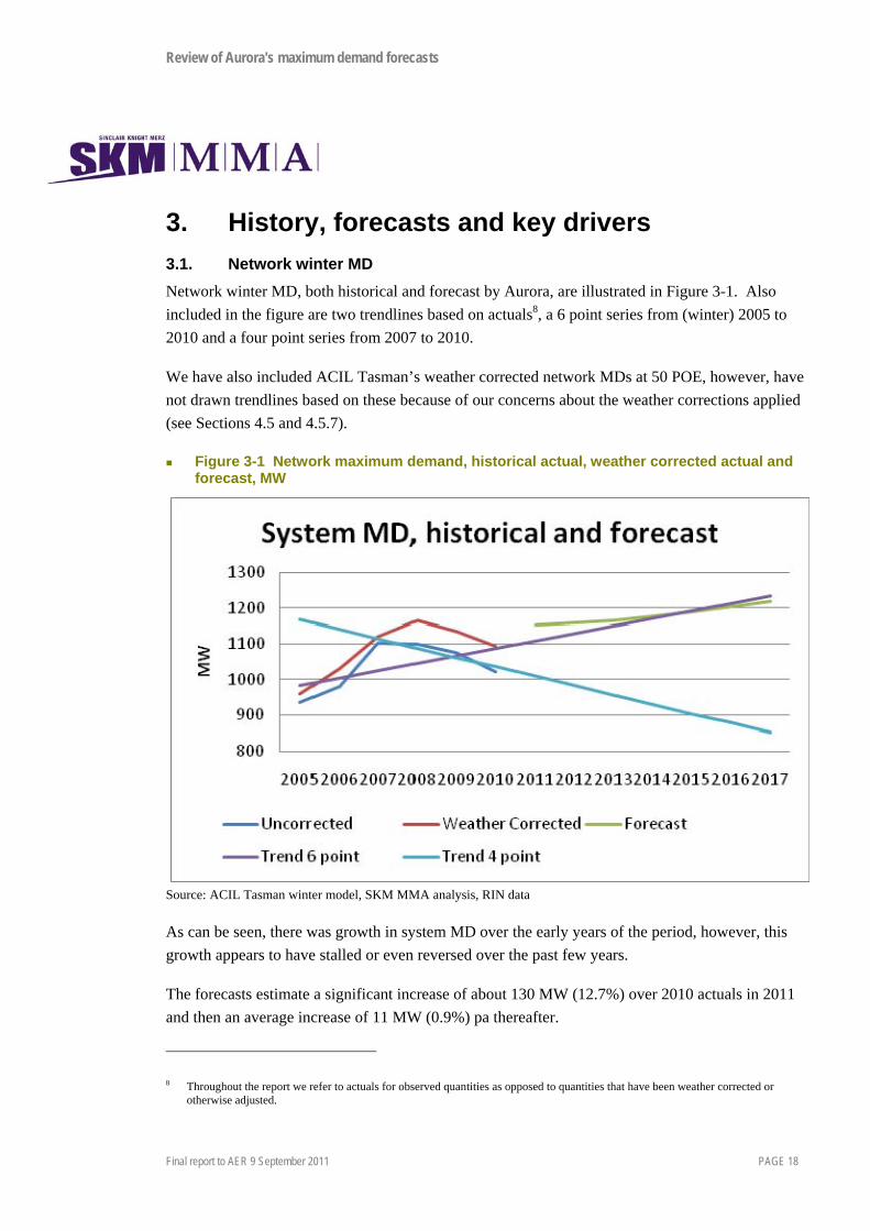
Network winter MD, both historical and forecast by Aurora, are illustrated in Figure 3-1. Also
included in the figure are two trendlines based on actuals8, a 6 point series from (winter) 2005 to
2010 and a four point series from 2007 to 2010.
We have also included ACIL Tasman’s weather corrected network MDs at 50 POE, however, have
not drawn trendlines based on these because of our concerns about the weather corrections applied
(see Sections 4.5 and 4.5.7).
Figure 3-1 Network maximum demand, historical actual, weather corrected actual and forecast, MW
Source: ACIL Tasman winter model, SKM MMA analysis, RIN data
As can be seen, there was growth in system MD over the early years of the period, however, this
growth appears to have stalled or even reversed over the past few years.
The forecasts estimate a significant increase of about 130 MW (12.7%) over 2010 actuals in 2011
and then an average increase of 11 MW (0.9%) pa thereafter.
8 Throughout the report we refer to actuals for observed quantities as opposed to quantities that have been weather corrected or otherwise adjusted.

Review of Aurora's maximum demand forecasts
Final report to AER 9 September 2011 PAGE 19
3.2. Non-coincident winter MD at terminal stations
Network MD will vary according to a number of variables including weather and the level of
coincidence of maximum demand at the different connection points or terminal stations in any
year. In order to eliminate the influence of the last factor, we find it instructive to consider not just
the system coincident MD, but the sum of the non-coincident MDs at terminal stations.
The history and forecast sum of non-coincident MDs for all terminal stations are illustrated in
Figure 3-2. Again we have included the six point and four point trendlines based on actuals and
ACIL Tasman’s historical weather corrected network MDs at 50 POE.
Figure 3-2 Sum of terminal station maximum demand, historical actual, weather corrected actual and forecast, MW
Source: ACIL Tasman winter model, RIN data, SKM MMA analysis
As for the system MD, there was growth in non-coincident MDs over the early years of the period
but not over the past few years. Again, the forecasts project an increase of about 150 MW (12.8%)
over 2010 actuals in 2011 and then an average of 12 MW (0.9%) pa thereafter.
The two obvious questions that arise from this initial assessment are:
Is the initial expected jump of about 12% from 2010 actuals realistic?

Review of Aurora's maximum demand forecasts
Final report to AER 9 September 2011 PAGE 20
Will growth history be more similar to that over the period 2005 to 2010 or over the period
2007 to 2010 or be intermediate between the two?
In order to assess the answers to such questions, it is important to consider the key drivers which
have impacted on the network over the past several years, and those that are expected to be in place
over the coming period.
3.3. Key drivers
The apparent key drivers of maximum demand historically and likely to apply over the next
regulatory period are:
Weather
Demographic considerations, population growth and household size
Economic factors, including state economic growth and household disposable income
Government policies
Pricing
Competing fuels
3.4. Weather
3.4.1. Weather correction
Maximum demand in winter is, at most terminal stations, inversely related to temperature, as the
temperature reduces the heating load increases. According to most methodologies, maximum
demand is calculated for the 50 POE, 10 POE and 90 POE temperatures, that is the(for winter)
minimum temperatures which would expect to be reached, on average, one year in two or one year
in ten or nine years in ten. As most terminal points are expected to reach a maximum load on
weekdays, the minimum temperature reached on weekdays in any year is normally compared
against the minimum temperature that would be expected to be reached based on long-term weather
data.
ACIL Tasman has assessed the weather sensitivity of terminal stations against the average of the
daily maximum and minimum at 11 weather stations. Three weather stations relate to connections
points which account for about 80% of Aurora’s maximum demand, station 94029 Hobart (Ellerslie
Road) about 35%, station 91126 Devonport Airport about 25% and station 91027 Launceston about
20%.
Using the history of the past 20 years, where possible, as the indicator of “normal” (see also
Sections 3.4.2 and 4.5 below), we have assessed indicatively the impact of weather on the peak day

Review of Aurora's maximum demand forecasts
Final report to AER 9 September 2011 PAGE 21
across the network, on a weighted average basis for the non-coincident peaks, over each year of the
period 2005 to 2010. This is described in Table 3-1.
Table 3-1 Description of the past 6 winters and indicative network impact
Winter of Year Description of weekday minimum across network
Indicative network impact
2005 Somewhat cooler than normal +7 MW (actual demand is higher than would be expected under normal weather by the order of 5 - 10 MW).
2006 Somewhat milder than normal -10 MW (actual demand is lower than would be expected under normal weather by the order of 10 MW.
2007 Somewhat cooler than normal +15 MW (actual demand is higher than would be expected under normal weather by the order of 15 MW.)
2008 Warmer than normal -21 (actual demand is lower than would be expected under normal weather by the order of 20 MW.
2009 Much warmer than normal -22 (actual demand is lower than would be expected under normal weather by the order of 20 - 25 MW.)
2010 Very much warmer than normal -28 (actual demand is lower than would be expected under normal weather by the order of 30 MW.
Note: indicative SKM MMA assessment based on ACIL Tasman derived average daily temperature sensitivities for estimated “normal” weather over the period 1991 to 2010 and coldest average temperature on a weekday in each year and a non-coincident basis. The minimum average daily temperatures on weekdays over the past 3 years have been warmer
than would be expected, significantly so over the past two years. This means that the actuals
recorded for the past three years need to be corrected up by of the order of 20 – 30 MW.
While we stress that these estimates of weather correction are indicative only, and applied on the
non-coincident demand, their order of magnitude is for
the difference between the 50 POE and 90 POE (very mild) values for the year 20119.. As a result
we consider the indicative values derived above to appear realistic. An analysis which uses daily
system MD and temperature data and weather simulation is expected to result in a significantly
more accurate 50 POE MD.
9

Review of Aurora's maximum demand forecasts
Final report to AER 9 September 2011 PAGE 22
3.4.2. Changing weather
Tasmania, as elsewhere across Australia, has experienced warming weather over the past ten or
twenty years. The history of winter minimum average day temperatures for four weather stations
with a reasonably long history is provided in Figure 3-3. As can be seen, there is an upward trend
for each of these stations.
Figure 3-3 Annual minimum winter day temperatures (average of maximum and minimum) over the past 50 or so years at four weather stations, Degrees C
Source: Data from ACIL Tasman winter model. The median of the minimum average temperatures (including both workdays and weekends)for the
longer term for Hobart (51 years), Devonport (20 years) and Launceston (31 years) weather
stations and over the past 20 and ten years is illustrated in Figure 3-4.

Review of Aurora's maximum demand forecasts
Final report to AER 9 September 2011 PAGE 23
Figure 3-4 Median minimum average temperature over the longer term (51 years for Hobart, 20 years for Devonport, 31 years for Launceston), 20 years and 10 years, Degrees C
Source: Data from ACIL Tasman winter model.
The minimum average temperature has increased from the longer-term to the 20 year and from the
20 year to the 10 year medians in Hobart and Launceston and from the 20 to 10 year median values
in Devonport for which only 20 years of data is available. The differences between the longer-term
and 20 year medians are significant at the 5% confidence level for Hobart and Launceston and the
differences between 20 and 10 year medians are statistically significant at the 5% level for
Devonport and Launceston and almost so for Hobart.
In its 2010 and 2011 assessments for Transend10, NIEIR has reviewed percentiles for the lowest
average temperature days according to four methods:
With a warming trend, weekends included
With a warming trend, weekends excluded
No warming trend, weekends included
No warming trend, weekends excluded.
10 See for example the National Institute of Economic and Industry Research (NIEIR) report to Transend, “Electricity sales and maximum demand forecasts for Tasmania to 2042” May 2011, page 14.

Review of Aurora's maximum demand forecasts
Final report to AER 9 September 2011 PAGE 24
NIEIR has implied that it considers the correct minimum temperature assumption to use is that
determined by incorporating a warming trend and excluding weekends (as the Tasmanian peak
never falls on a weekend)11. If a warming trend is assumed, then the impact will be to again
moderate growth in winter maximum demand.
In the ACIL Tasman report on energy consumption, heating degree days (HDD) is defined as the
sum of the number of degrees below 18 of the average daily temperature. This value is commonly
used when assessing the “coldness” of a day or season and the consequent need for heating and
also in assessing seasonal weather impact on energy consumption. Figure 3-5 shows that for the
Hobart weather station the measure of HDDs has been declining over the available history, leading
to more mild winters in recent years.
Figure 3-5 Heating Degree Days for Hobart Winters 1960-2010
ACIL Tasman has forecast energy consumption on the basis of a reducing trend of HDD over
time12.
Thus, there is evidence that the weather in Hobart has become milder over the past 20 years both in
terms of the coldest days and the coldness of seasons generally.
11 National Institute of Economic and Industry Research (NIEIR) report to Transend, “Electricity sales and maximum demand forecasts for Tasmania to 2042” May 2011, pages 25 and 43.
12 ACIL Tasman report to Aurora Energy, “Energy consumption forecasts: 2010-11 to 2016-17”, June 2011, page 23.
600
650
700
750
800
850
900
950
1000
1960
1963
1966
1969
1972
1975
1978
1981
1984
1987
1990
1993
1996
1999
2002
2005
2008
Hobart Winter HDD
Year
Hobart Winter HDD

Review of Aurora's maximum demand forecasts
Final report to AER 9 September 2011 PAGE 25
3.5. Population and customer number growth
According to the Australian Bureau of Statistics (ABS)13 Tasmanian population has grown by
about 0.86% pa between 2005 and 2010. ACIL Tasman has assumed that it will grow at a slower
rate, some 0.633% between 2010 and 2017, based on the ABS Population projections, series B14.
This growth rate is a little lower than that forecast recently by KPMG
which has projected population growth between 2010 and 2017
estimated at 0.8% pa15.
ACIL Tasman has estimated a linear relationship between population growth and customer number
growth16, with a growth of 1 customer for each increase of 2.5 in population, approximately in line
with average household numbers.
Residential customer number growth is often approximated by the growth in dwellings or housing.
NIEIR has estimated dwelling growth over the period 2010 to 2017 to be some 0.15% pa higher
than the growth rate of population17 (suggesting a reduction in persons per dwelling). Conversely,
the KPMG 2010 forecasts for AEMO have estimated housing growth to be a little less than the
growth in population. On balance, the ACIL Tasman expectation that the growth rate in customer
numbers is proportional to that in population appears reasonable.
As a result, the growth of residential customers would be expected to be of the same order as, or a
little lower than it was over the period 2005 to 2010.
3.6. Economic growth
State economic growth as measured by Tasmanian Gross State Product (GSP) grew by about 2.7%
pa between 2005 and 201018. However, GSP growth in 2010 was estimated to be about 0.4%.
Aurora refers to the link between economic growth and demand and also expectations about
economic growth over the coming regulatory period in its Regulatory Proposal:
“A peak in growth occurred during 2008-09, prior to the global financial crisis (GFC), and fell
during the 2009-10 and 2010-11 years. While growth had declined during this period, capital
expenditures continued to rise as Aurora completed projects instigated during the period
13 Australian Bureau of Statistics, Catalogue 3101.0, Australian Demographic Statistics, Estimated Residential Population, 2011 14 ACIL Tasman report to Aurora Energy, “Energy consumption forecasts: 2010-11 to 2016-17”, June 2011, page 23. 15
We have assumed linear growth between 2015 and 2020. 16 ACIL Tasman report to Aurora Energy, “Energy consumption forecasts: 2010-11 to 2016-17”, June 2011, page 34. 17 National Institute of Economic and Industry Research (NIEIR) report to Transend, “Electricity sales and maximum demand
forecasts for Tasmania to 2042” May 2011, page 7. We have assumed linear growth between 2015 and 2020. 18 Australian Bureau of Statistics, Catalogue 3101.0, Australian Demographic Statistics, Estimated Residential Population, 2011

Review of Aurora's maximum demand forecasts
Final report to AER 9 September 2011 PAGE 26
immediately prior to the GFC. It is expected that growth will recover during the 2011-12 financial
year and increase at subdued levels of less than 1 percent over the foreseeable future19.
“At the time of the last Distribution Determination, Tasmania had experienced an extended period
of unprecedented economic growth. The economic recovery that commenced in 2001-02 was
continuing to show above trend economic growth, supported by strong jobs growth, public and
private sector investment close to record levels, high levels of consumer spending and growth in
export sales. The unemployment rate was at a record low, one half of the level it had been a decade
previously. This trend has continued through the current Regulatory Control Period, despite the
significant slow-down in the world and national economies in 2008 and 2009 as a result of the
global financial crisis. This is consistent with past economic cycles where there has usually been a
lag between changes in national economic conditions and changes in the Tasmanian economy.
Tasmania also benefited proportionally more than most other jurisdictions from the Australian
Government’s Nation Building – Economic Stimulus Plan as a higher proportion of Tasmanian
households are on lower incomes and receive welfare payments.
During 2010, the Tasmanian economy experienced a slowdown as the stimulus was withdrawn and
is emerging from the global economic downturn at a weaker pace than Australia as a whole.
Private investment remains weak and is likely to remain so in the near term. Tasmanian
employment is yet to recover to pre-crisis levels, unlike other jurisdictions.
The Australian Government’s recent Mid-Year Economic and Fiscal Outlook stated that:
“as fiscal stimulus is withdrawn, private-sector led growth is taking hold, with business investment
and commodity exports emerging as the key drivers of growth” .
To date, this has not been the case in Tasmania, and the State’s growth is unlikely to keep up with
national growth” 20.
In its forecasts of energy consumption21, ACIL Tasman has projected economic growth to be
subdued, averaging some 2% pa over the period 2010 to 2017.
However, in the 2010 and 2011 NIEIR forecasts for Transend, economic growth has been taken to
be that from the KPMG forecasts, some 2.4% to 2.5% pa on average.
Historical GSP growth rates and those projected by ACIL Tasman and KPMG in 2011 are
illustrated in Figure 3-6.
19 Aurora Energy Regulatory Proposal, page 3. 20 Aurora Energy Regulatory Proposal, page 11 with footnotes excluded. 21 ACIL Tasman report to Aurora Energy, “Energy consumption forecasts: 2010-11 to 2016-17”, June 2011, pages 19 and 43.

Review of Aurora's maximum demand forecasts
Final report to AER 9 September 2011 PAGE 27
Figure 3-6 Historical and forecast growth in Tasmanian Gross State Product, %
GSP growth from 2010 to 2017 is projected to be lower than the 2.7% pa growth seen over the
period 2005 to 2010. According to the KPMG forecasts used by NIEIR in 2011, growth will
average some 2.4% pa while according to the ACIL Tasman forecasts it will be some 2% pa. The
forecast GSP growth rates are some 8% to 25% lower than those seen over the period 2005 to
2010.
3.7. Government policies
A range of Government policies, both federal and state, have been adopted over recent years which
are expected to impact on electricity usage. These include:
Energy efficiency opportunities program which impacts on larger energy users
Minimum Energy Performance Standards on appliances
National framework for energy efficiency
Building energy standards and disclosure
Phase out of incandescent lights
Photovoltaic subsidies and feed-in tariffs
Solar hot water subsidies and feed-in tariffs
Carbon pricing from July 2012 pending the passing of Federal legislation (see pricing
impact in Section 3.9 below).
GSP growth, historical and forecast
0.0%
1.0%
2.0%
3.0%
4.0%
5.0%
2003
2005
2007
2009
2011
2013
2015
2017
Historical
ACIL Tasman
KPMG/NIEIR
Review of Aurora's maximum demand forecasts
Final report to AER 9 September 2011 PAGE 28
While the impacts of each of these has not been quantified, each is likely to lead to reduced
electricity usage, some also to reduced maximum demand.
3.8. Gas supply and reticulation
Gas supply to Tasmania commenced in August 2002, significantly later than to most other states in
Australia. While most of the gas used in Tasmania is for power generation, some is also used by
industrial, residential and commercial users.
Reticulation to residential and commercial customers commenced in 2004. By 2009/10 some 2 PJ
of natural gas was reticulated to customers in Tasmania, including to about 7,500 residential
customers each consuming about 40 GJ of gas pa, mainly for heating and hot water and about 600
commercial and industrial customers. In addition, a further 2 PJ or so is supplied directly to larger
consumers in Tasmania.
While much of the gas used has displaced liquid fuels for industry and, in the residential sector,
wood for heating, some is also displacing electricity. In addition, cogeneration at locations such as
Launceston General Hospital, the Fonterra cheese factory at Wynyard and the Simplot vegetable
processing plant near Ulverstone have or will act to displace electricity usage and dampen growth
in electricity usage.
Gas demand projections in the 2010 Gas Statement of Opportunities (GSOO)22 suggest that gas
demand in Tasmania for purposes other than power generation will continue to grow between 2010
and 2017, with growth rates ranging from 2.4% pa to 10.5% pa, depending on scenario.
3.9. Price effects
As for much of Australia, there have been significant increases in electricity prices in Tasmania
over recent years, and more are expected as the carbon price is introduced. According to NIEIR23,
the increases have been or are expected to be:
% in real terms for residential consumers between 2005 and 2010 and a real reduction of
% for business customers
% in real terms for both residential and business customers
These increases are expected to dampen demand for electricity compared to that experienced over
the period 2005 to 2010. Aurora has commented that it believes price impacts account for some of
the reduced demand growth in recent years24.
22 Gas Statement of Opportunities 2010 Chapter 5 demand projections download available from http://www.aemo.com.au/planning/gsoo2010.html.
23 National Institute of Economic and Industry Research (NIEIR) report to Transend, “Electricity sales and maximum demand forecasts for Tasmania to 2042” May 2011, page 20.

Review of Aurora's maximum demand forecasts
Final report to AER 9 September 2011 PAGE 29
3.10. Summary of key drivers expected over the period
The key drivers we have considered are similar to those considered relevant in reports by ACIL
Tasman and NIEIR. Based on this assessment, we would expect that the past three years of actuals
would be weather corrected upwards by some 20-30 MW as minimum winter temperatures have
been unusually mild.
Beyond this impact, however, most of the key drivers we have considered, population and dwelling
growth, economic growth, government policy effects and price impacts all suggest that growth over
the period 2011 to 2017 should be lower than it was over the period 2005 to 2010.
24 Meeting between Aurora, AER, ACIL Tasman and SKM MMA on 14 July 2011.

Review of Aurora's maximum demand forecasts
Final report to AER 9 September 2011 PAGE 30
4. Aurora’s MD forecasting methodology at system, Terminal Station and Zone Substation levels
4.1. Overview
Prior to submitting its Proposal, Aurora commissioned ACIL Tasman to produce winter and
summer MD forecasts at the TS and ZSS levels. These forecasts were the basis of the MD
information provided at system, TS and ZSS levels in the RINs and in the Aurora MD forecast
document25 .
SKM MMA has primarily reviewed the ACIL Tasman forecasts as contained in the RINs. Aurora
has provided the ACIL Tasman models to the AER in confidence and has also explained the
forecasts for one TS and one ZSS in some detail.
However, the AER has subsequently been informed that all growth-related projects at feeder level
were prepared based on the Utility Engineering Solutions (UES) growth forecasts prepared in
200826. Aurora has also stated that it considers these forecasts to be reasonably consistent with the
ACIL Tasman forecasts27.
SKM MMA has primarily been asked to review the ACIL Tasman forecasts at TS and ZSS levels
to assess whether these are reasonable. However, SKM MMA has then compared UES growth
rates against those produced by ACIL Tasman to assess whether these are likely to be consistent
with the ACIL Tasman forecasts after taking into account comments resulting from the review.
This Chapter looks at the methodologies used by ACIL Tasman to forecast at the system,
connection point and zone substation levels. The next Chapter looks at forecasts at the feeder level.
4.2. Basis of review
SKM MMA has reviewed the methodology described and applied by ACIL Tasman for forecasting
the demands at TS and ZSS. This review is based on the descriptions in the Regulatory Proposal,
the ACIL Tasman methodology report28 and Load Forecast Report29 and the Winter Aurora Model
v44 spreadsheets30 provided as well as discussions between Aurora, AER and SKM MMA on
25 Aurora Energy, “2010 distribution network connection maximum demand forecast” Issue 1.0 December 2010. 26 Utility Engineering Services (UES) report to Aurora Energy, “2008 distribution network ten-year consumption and maximum
demand forecasts”, December 2008. 27 Meeting between Aurora, AER, ACIL Tasman and SKM MMA on 14 July 2011. 28 Document AEO61 ACIL Tasman load forecasting methodology: ACIL Tasman report to Aurora, “Outline of Aurora’s spatial
demand forecasting methodology”, September 2010 29 AE057 – ACIL Tasman Load Forecast CONFIDENTIAL.pdf, primary attachment to the regulatory proposal 30 NW-#30185879-v1-Winter_Aurora_model_v44 COMMERCIAL IN-CONFIDENCE.xlsx, provided on June 23rd

Review of Aurora's maximum demand forecasts
Final report to AER 9 September 2011 PAGE 31
14 July 2011. We have focused on the winter maximum demand as almost all locations in
Tasmania are winter peaking.
We have reviewed the methodology as described and its application by ACIL Tasman and/or
Aurora. A summary of the methodology with brief comments on both methodology and
application is presented in Table 4-1. A more detailed review follows in Section 4.3.
Table 4-1 Summary of methodology and brief comments
Step ACIL Method Output SKM MMA comment on method
SKM MMA comment on application
0 Historic Daily MD
Select the daily MD for winter and summer.
Daily MD for each station
Ok as long as errors and temporary transfers are filtered.
1 Temperature Sensitivity
Determine the temperature sensitivity for each TS each year using the daily MD and local weather station. Excludes weekends
Temperature sensitivity MW/°C for each TS for each year
Choice of weather variable is important.
Ignores the quality of the temperature sensitivity regression fit
2 Standard Weather
ACIL selects the day of coldest average temperature from each winter, then calculates the 50th and 10th percentile. Includes non-workdays. As standard, ACIL also uses a long-term distribution, despite evidence that the past 10 and 20 years have seen significant warming.
10 and 50 POE temperature for each weather station based on long-term temperatures
Weekends should not be included in step 1 if it has been decided that the maximum demand does not occur on a weekend. The long-term averages are unlikely to be appropriate given the difference of the past 20 years compared to the previous 20 years. SKM MMA recommends using a 20 year history.
ACIL is slightly overestimating the 10 and 50 POE weather by including weekends when calculating the standard weather and further by using a long-term average as the standard.
3 50 POE MD Take the actual maximum demand recorded each winter and adjust by the difference between the actual temperature on the day of maximum demand and the 50 POE temperature
Temperature Corrected History
This approach will generally over-estimate the 50 POE MD.
Weather correction is likely to be overstated. Over the past 6 years ZSS MDs
Review of Aurora's maximum demand forecasts
Final report to AER 9 September 2011 PAGE 32
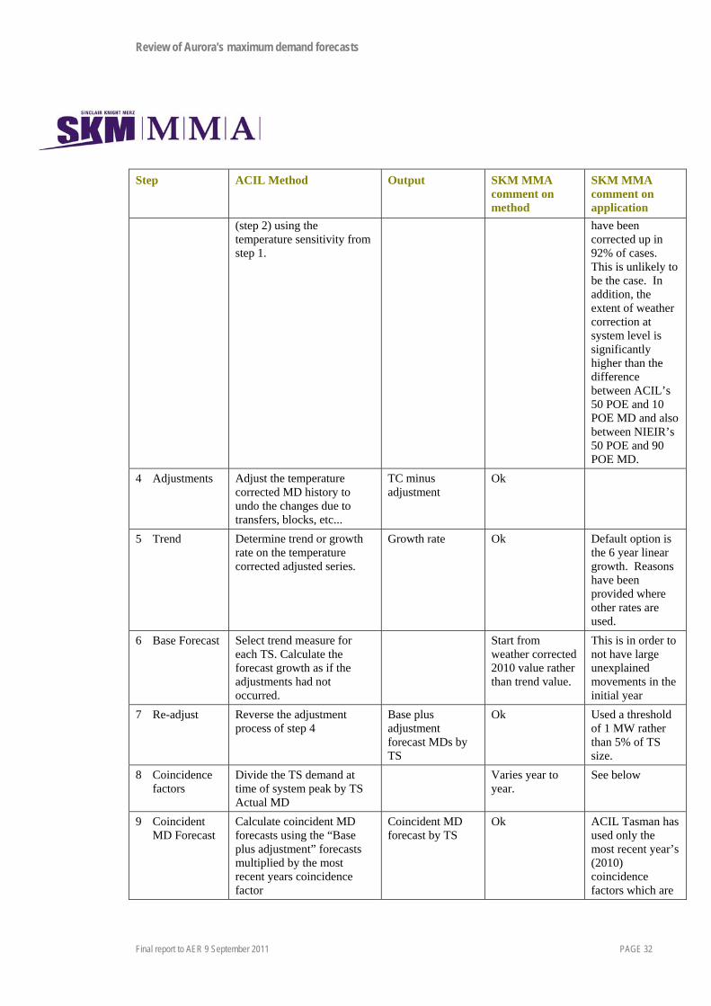
Step ACIL Method Output SKM MMA comment on method
SKM MMA comment on application
(step 2) using the temperature sensitivity from step 1.
have been corrected up in 92% of cases. This is unlikely to be the case. In addition, the extent of weather correction at system level is significantly higher than the difference between ACIL’s 50 POE and 10 POE MD and also between NIEIR’s 50 POE and 90 POE MD.
4 Adjustments Adjust the temperature corrected MD history to undo the changes due to transfers, blocks, etc...
TC minus adjustment
Ok
5 Trend Determine trend or growth rate on the temperature corrected adjusted series.
Growth rate Ok Default option is the 6 year linear growth. Reasons have been provided where other rates are used.
6 Base Forecast Select trend measure for each TS. Calculate the forecast growth as if the adjustments had not occurred.
Start from weather corrected 2010 value rather than trend value.
This is in order to not have large unexplained movements in the initial year
7 Re-adjust Reverse the adjustment process of step 4
Base plus adjustment forecast MDs by TS
Ok Used a threshold of 1 MW rather than 5% of TS size.
8 Coincidence factors
Divide the TS demand at time of system peak by TS Actual MD
Varies year to year.
See below
9 Coincident MD Forecast
Calculate coincident MD forecasts using the “Base plus adjustment” forecasts multiplied by the most recent years coincidence factor
Coincident MD forecast by TS
Ok ACIL Tasman has used only the most recent year’s (2010) coincidence factors which are

Review of Aurora's maximum demand forecasts
Final report to AER 9 September 2011 PAGE 33
Step ACIL Method Output SKM MMA comment on method
SKM MMA comment on application
lower than average. In forecasts we consider the average over a number of years should be used.
10 Reconcile to System Coincident forecast
Sum of coincident forecast MDs against NIEIR forecast of Aurora system MD
Reconciled Coincident Forecasts by TS Reconciliation factor for each forecast year.
Ok We have concerns about the use of forecasts which have not been validated as suitable for the purpose, use different key drivers and assume a very significant increase in year one. Aurora relies very heavily on system reconciliation and to correct for any other methodological issues such as weather correction.
11 Non-coincident reconciled MD
Divide the reconciled coincident forecast by the coincidence factor used in step 9.
Reconciled Non-coincident MD
Ok We consider that forecasts need to use the average coincidence factor over a number of years, not that from the most recent year. Using a lower coincidence factor than average will inflate non-coincident forecasts.
12 Non-coincident reconciled MVA
Convert MD to MVA using power factor
Reconciled Non-coincident MVA for each TS
Ok Have used the PF from the most recent year.

Review of Aurora's maximum demand forecasts
Final report to AER 9 September 2011 PAGE 34
4.3. Review of Methodology Steps
Steps 1, 2 and 3, related to standard weather and weather correction, are discussed in detail in
Section 4.5, where we review as a whole the historic weather corrections for TS and ZSS.
4.3.1. Capturing Daily MD for each substation
Aurora records the daily MD for each substation for every day of summer and winter. This is
standard practice and considered reasonable as long as there is some process for checking any
anomalous data points for SCADA errors or temporary load transfers between substations. We
understand that temporary transfers between locations are not very common in Tasmania compared
to other states. Only workdays are considered likely to be the maximum demand day.
4.3.2. Adjustments due to block loads, transfers, embedded generation - Steps 4 and 7
ACIL has adjusted the weather corrected historic sequence to back out the changes due to transfers,
blocks load, irrigation loads and embedded generation. There is no demand side management and
little embedded generation31. This results in a sequence of expected historic MDs as if those
changes had never occurred. Later in step 7 these adjustments are reversed. The goal is to remove
the image of these one-off items from the trend growth derived in step 5.
New residential subdivisions are considered part of organic growth and not explicitly added as
block loads due to the slow growth seen in Tasmania. Block loads are only included in the forecast
when they are committed and a payment has been made. In general, Aurora has few new block
loads forecast and has provided some detail about these.
In general, this methodology is good practice and well applied however, there are some caveats.
Firstly, with block loads ACIL has applied a threshold of 1 MW, we consider a threshold based on
the capacity of the TS or ZSS a more appropriate measure. For many of the larger TS or ZSS in the
Aurora network a 1 MW block load is well under 5% of the total load and should probably be
included as part of trend growth. While a 1 MW threshold is acceptable, we suggest that a
threshold size of 5% of the capacity of the substation is more robust. However, the 1 MW
threshold is considered reasonable so long as consistently applied.
Secondly, when we review the winter forecast spreadsheets we note that the transfers in certain
years do not net to zero. For example, in 2007 the transfers in the Tamar region are 11 MW on to
Hadspen and 8 MW off Norwood, so a net 3 MW has appeared. Similarly in the Hobart West
region a net 20 MW appears due to transfers in 2007. ACIL/Aurora have explained that these
31 During the meeting on 14 July, ACIL/Aurora did mention there was a mistake made with the embedded generation at Derby. This is, however, unlikely to be material unless growth capex is to be spent there.

Review of Aurora's maximum demand forecasts
Final report to AER 9 September 2011 PAGE 35
situations usually occur when a new substation is established but it is still not clear why there
should be a net transfer.
A further issue with load transfers is that it is assumed that these have no growth associated with
them and that all growth due to that set of customers or load prior to the transfer will be left
associated with the sending substation. We recognise that some load transfers will be expected to
have no further load growth, however we would expect some consideration to be given to treating
transfers differently, depending on the nature of the customer types transferred. Nevertheless, in
terms of magnitude of impact on final demand forecasts of the load growth of transfers is unlikely
to be material.
4.3.3. Trends and Base Forecast Steps 5 and 6
The base forecast is comprised of two components a growth rate and a starting point.
4.3.3.1. Growth Rates
ACIL derives a set of trend growth rates for each TS and ZSS based on the weather corrected
historic MDs which have been adjusted to remove the impact of transfers, block loads and
embedded generation. This is an appropriate series to determine the growth rates from.
ACIL calculates both the linear (MW) and compound (percentage) growth rates for 2, 3, 4, 5 and 6
year histories for which the data is available. For each substation one of these growth rates is
selected and applied. The default option is to use as many years as possible, the 6 year linear
growth rate. We consider this to be reasonable for up to six years. Given the changing nature of
many ZSS, using a linear growth rate for a much longer time horizon may be problematic. In some
cases a different growth rate is selected and in general these choices have been explained during the
meeting with Aurora and ACIL on 14 July.
For seven of the TS a growth rate of zero has been applied. These are predominantly small isolated
locations where no organic growth is expected and the MD histories can be volatile.
ACIL has applied zero growth rates to all of the ZSS forecasts. This occurs because the ZSS
forecast demand growths are based on the growth for the relevant Terminal Stations.
4.3.3.2. Starting Point
The starting point for each substation MD forecast sequence is the 2010 weather corrected MD.
ACIL has explained that this was done to avoid large discontinuity with the historic series. We
consider this choice to be reasonable, especially given recent changes apparent at system level.

Review of Aurora's maximum demand forecasts
Final report to AER 9 September 2011 PAGE 36
4.3.4. Coincidence Factors step 8
ACIL calculates the coincidence factor here as the substation demand at time of system peak
divided by the substation non-coincident peak.
ACIL has included within its methodology the choice of using the average of any of the single,
two, three or five year averages of coincidence factors or a linear trend of the 5 year history. In its
methodology report32, ACIL Tasman has stated that it will most probably use either a three or five
year average diversity factor.
However, of these sets of coincidence factors calculated ACIL has used the single year history of
the most recent year 2010. This was a very mild winter and therefore the peaks appear to be less
correlated (more diverse) than usual. The weighted average coincidence across all TS was 0.92 at
the time of system peak in 2010, the average over 3, 5 and 6 years is 0.94 (see Figure 4-1).
Figure 4-1 Average coincidence factor calculated over varying periods
Source: Uncorrected RIN system MD divided by sum of non-coincident TS MD and averaged over x years
This means that when Aurora reconciles to the NIEIR coincident system forecast going forward,
the sum of ZSS coincident MDs ACIL is using is likely to be around 2-3% higher than would have
been the case if an average of 3, 5 or 6 years was used. This leads to an average reconciliation
32 Document AEO61 ACIL Tasman load forecasting methodology: ACIL Tasman report to Aurora, “Outline of Aurora’s spatial demand forecasting methodology”, September 2010, page 5.

Review of Aurora's maximum demand forecasts
Final report to AER 9 September 2011 PAGE 37
adjustment of all ZSS that is some 2.5% larger than we consider reasonable. While this is not of
relevance at the system coincident level, we consider it will inflate the forecasts at the non-
coincident level, on which capex forecasts are based, by some 2.5% pa in each year.
The choice of coincidence factors to use depends upon a number of considerations, including the
available history, whether the network (and thus the associated coincidence factors) is undergoing
change, and whether coincidence factors are likely to be significantly affected by unusual weather.
We recommend using a period significantly longer than the most recent year or two which are
likely to have been affected by mild winter weather. As the three, five and six year coincidence
factor averages are very similar and ACIL Tasman has calculated five year averages, we consider
the five year average a reasonable coincidence factor to use. For any substations that appear to
have a clear trend of increasing or declining coincidence it might be necessary to investigate the
drivers and their likely future impacts and possibly using a linear trend to forecast the coincidence
factor.
4.3.5. Reconciliation to NIEIR steps 9 to 11
The coincidence factors determined in step 8 are used to calculate the forecast non-reconciled
coincident substation MDs.
Then, according to the meeting on July 14th, Aurora has taken a decision that the forecasts need to
be reconciled against forecasts derived from NIEIR. According to ACIL Tasman33:
“Reconciliation with an independently produced system level forecast has the advantage of
allowing the methodology to incorporate the impacts of broader macroeconomic and
demographic aggregates, as well as the impacts of new policy initiatives which are better
modelled at the system level. System level data is also smoother and more amenable to the
fitting of econometric models which can be used to generate more accurate system level
forecasts.”
The reconciliation process undertaken by ACIL Tasman is to calculate its own coincident system
maximum demand, compare this against the NIEIR derived system maximum demand and scale its
un-reconciled system coincident peak demand to the NIEIR system peak demand. The ACIL
un-reconciled system forecast and the coincident system forecast derived from the forecast based
on the NIEIR report to Transend, to which the ACIL forecasts have been reconciled and the scaling
applied to substations are provided in Table 4-2.
33 Document AEO61 ACIL Tasman load forecasting methodology: ACIL Tasman report to Aurora, “Outline of Aurora’s spatial demand forecasting methodology”, September 2010, page 5.

Review of Aurora's maximum demand forecasts
Final report to AER 9 September 2011 PAGE 38
Table 4-2 Reconciliation of NIEIR forecast with sum of substation coincident MDs
Year
Sum of ACIL Substation
Coincident (MW) NIEIR Forecast (MW) Scaling applied to
substations
2011 1115 1152 3.39%
2012 1127 1159 2.83%
2013 1142 1165 2.05%
2014 1154 1177 1.98%
2015 1167 1189 1.86%
2016 1179 1203 2.03%
2017 1192 1218 2.18%
Each substation has the same adjustment applied to reconcile to the NIEIR forecast. In all years
this requires an increase in substation forecast MD of between 1.86% and 3.4%. This same
adjustment factor is applied to the system coincident and non-coincident substation MD forecasts.
From a methodological viewpoint we consider reconciliation between spatial and global forecasts
to constitute good practice. There are, however, some important caveats. It is important that both
the spatial and global forecasts forecast the same thing, should have a common history and, most
importantly, have the same underlying key drivers. Any differences in starting point and growth
rate need to be carefully investigated and documented. In addition, it is important that both sets of
forecasts be prepared by credible forecasters who understand the system and recent history and
drivers. These issues are discussed in Section 4.6.
4.3.6. Conversion from MW to MVA in step 12
The final step involves converting from MW into MVA. The reconciled non-coincident substation
forecasts in MW are converted to MVA demands by using the power factor from the most recent
historic peak demand on the substation in 2010.
Power factors vary much less year to year than diversity factors so we consider it reasonable to use
this value from the most recent year. However, if it varies significantly from earlier years then
some justification for the choice made is required.
The reconciled non-coincident forecast demand in MVA is the expected maximum load placed in
the equipment at the substation and it to meet this requirement that capex planning is usually based.
However, in these forecasts as a constant power factor is assumed, they are not particularly
relevant.

Review of Aurora's maximum demand forecasts
Final report to AER 9 September 2011 PAGE 39
4.4. Summer peaking substations
There are several substations that are summer peaking. These are Waddamana, Avoca, Derby, Port
Latta, Smithton and Palmerston. The summer peak for most Tasmania substations is normally
associated with heating load (ie cold mornings). However, there are presumably a handful of
substations which because of larger industrial loads in summer or possibly air-conditioning loads,
peak in summer. We have not further investigated these stations.
4.5. Weather correction methodology and application
Daily maximum demand during winter is typically made up of three components; a (largely) fixed
component, a temperature sensitive component and a random scatter component. These can all be
estimated from the regressions ACIL Tasman has calculated. The annual MD often occurs when
there is a combination of both high temperature sensitive demand and a high positive random
scatter.
The random scatter in some situations may be due to a large variable load that is not directly
temperature sensitive (e.g. irrigation, some industrial) or it may just be due to random coincidence
in consumer behaviour.
4.5.1. ACIL Weather Correction Methodology
The following is a summary of the ACIL weather correction methodology for estimating historic
50 POE MDs:
For each TS and ZSS a linear regression is calculated for each historic year of average
temperature versus daily MD for each winter workday.
ACIL only uses the temperature sensitivity coefficient.
The regression is applied systematically without consideration for regression r-squared or by
examining the scatter plots such as those illustrated in Sections 4.5.1.1 and 4.5.1.2.
ACIL has noted that low regression r-squared outcomes are usually associated with low
temperature sensitivities and therefore smaller adjustments in load. If the temperature
coefficient is in the wrong direction it is taken to be zero.
ACIL has calculated the 50 POE MD by adjusting the maximum demand actually recorded to
a 50 POE temperature day. 50 POE = Max Demand + Temp Sens x (50 POE Temp – Temp on
day of Max Demand). See illustration in Figure 4-3.
Elsewhere in Sections 3.4.2 and 4.5 we discuss our understanding that weather has been
warming and the impacts of this on standard 50 POE temperatures. We consider that the
standard weather calculations need to take into account more recent warming and exclude
weekends as assessed in Section 4.5.6. Our 50 POE temperature estimates are based on the
most recent 20 years of weather.

Review of Aurora's maximum demand forecasts
Final report to AER 9 September 2011 PAGE 40
Note that the Scottsdale 50 POE temperatures used in the Winter Spreadsheet is incorrect
as it has included several years of missing data leading to a temperature of 3.7 degrees,
whereas the correct value is 4.5.
We do not consider this to be a reliable method for estimating historic 50 POE MD as it will
almost always overestimate the MD by assuming that the maximum temperature day should
always coincide with one of the largest positive scatter days.
4.5.1.1. ACIL 50 POE Historic MDs for Chapel St
The ACIL weather corrections for Chapel St are presented in Table 4-3. Figure 4-2 and Figure 4-3
provide example scatter plots of the regression analyses for Chapel Street in 2005 and 2010. The
weather correction process of adjusting the actual maximum demand day to the 50 POE
temperature is demonstrated in Figure 4-3, which highlights how far the 50 POE MD estimation
provided is from any of the actual demands in that year. We note that in winter 2005 there was a
workday with an average temperature below the long-term workday average, however due to the
scatter on other days it was not the maximum demand day.
Table 4-3 Chapel St Actual MD, ACIL 50 POE MD and Regression terms for 2005 to 2010
Chapel St Actual MD ACIL 50 POE MD
Temperature Sensitivity
Constant Term
Standard Error of Fit
R-squared
2005 51.54 53.37 -1.30 53.16 2.06 0.73
2006 52.61 57.62 -1.59 60.84 2.84 0.63
2007 43.57 44.46 -1.18 44.85 2.66 0.58
2008 45.20 47.49 -1.39 47.44 2.03 0.59
2009 42.31 47.03 -0.99 43.66 2.55 0.40
2010 41.08 45.99 -1.13 44.24 1.90 0.50

Review of Aurora's maximum demand forecasts
Final report to AER 9 September 2011 PAGE 41
Figure 4-2 Chapel St 2005 Winter, Daily MD and Daily Average Temperature regression
Figure 4-3 Chapel St 2010 Winter, Daily MD and Daily Average Temperature regression
y = ‐1.3037x + 53.163R² = 0.7303
20
25
30
35
40
45
50
55
60
0 2 4 6 8 10 12 14 16 18 20
Daily M
axim
um Dem
and (M
W)
Daily Average Temperature
Chapel St 2005 Winter
2005
ACIL 50 POE
Linear (2005)
y = ‐1.129x + 44.237R² = 0.4959
20
25
30
35
40
45
50
0 2 4 6 8 10 12 14 16
Daily M
D (MW)
Daily Average Temperature
Chapel St 2010 Winter
2010 Daily
ACIL 50 POE
Linear (2010 Daily)

Review of Aurora's maximum demand forecasts
Final report to AER 9 September 2011 PAGE 42
As shown in Figure 4-3 the ACIL weather correction methodology is to adjust the maximum
demand day to the 50 POE temperature, which ACIL Tasman calculates as 4 degrees for Hobart
(Ellerslie Road). The slope of the adjustment is determined from the regression fit for all winter
days.
4.5.1.2. ACIL 50 POE Historic MDs for Geilston
The ACIL Tasman weather corrections for Geilston Bay are presented in Table 4-4. An example
of a scatter plot of daily MD against daily average temperature for Geilston Bay in 2010 is
presented in Figure 4-4.
Table 4-4 Geilston Actual MD, ACIL 50 POE MD and Regression terms for 2006 to 2010
Year Actual MD ACIL 50 POE MD
Temperature Sensitivity
Constant Term
Standard Error of Fit
R-squared
2006 25.19 28.35 -1.00 30.31 1.63 0.67
2007 31.14 31.79 -0.87 31.50 1.63 0.67
2008 29.27 31.08 -1.07 34.79 1.41 0.64
2009 26.97 28.30 -0.81 30.28 1.22 0.66
2010 26.35 28.55 -0.90 30.86 1.47 0.51
Figure 4-4 Geilston 2010 Winter, Daily MD and Daily Average Temperature regression
y = ‐0.8986x + 30.858R² = 0.5108
15
17
19
21
23
25
27
29
31
0 2 4 6 8 10 12 14 16
Daily M
D (MW)
Daily Average Temperature
Geilston Winter 2010 MDs
Daily MDs
ACIL 50 POE
Linear (Daily MDs)

Review of Aurora's maximum demand forecasts
Final report to AER 9 September 2011 PAGE 43
4.5.2. SKM MMA Approach to 50 POE weather correction
As stated previously daily MD is generally made up of three components:
1) A fixed component
2) A temperature sensitive component
3) A random scatter component.
Based on our experience, the annual MD usually occurs when there is a combination of both cold
weather and a high positive random scatter.
4.5.2.1. Basic 50 POE MD calculations
Using the first two components, the fixed and temperature sensitive loads we can calculate what we
refer to as the “basic” 50 POE.
Basic 50 POE = Fixed Load + Temperature Sensitivity x 50 POE Temperature
Our experience is that this approach will tend to underestimate the actual 50 POE because it
doesn’t allow for the fact that the random scatter may result in MDs above the regression line at
temperatures below the 50 POE temperature (see for example, Figure 4-2 to Figure 4-4).
4.5.2.2. Basic plus “scatter”
A more comprehensive approach is to include the impact of the random scatter term. This can be
determined from the standard error to the regression fit.
50 POE Basic plus “Scatter”= Fixed Load + Temperature Sensitivity x 50 POE Temperature +
A x Standard Error of Regression fit
This still makes the assumption that the maximum demand day will correspond to the maximum
temperature day which is expected to be 50 POE. It is not clear how much of the standard error
scatter to expect on a given day.
This is very similar to the approach taken by ACIL however, ACIL assumes that the scatter term is
equal to the scatter on the maximum demand day. This is often the largest scatter term for any day
near the coldest temperature and can be several times larger than the standard error to the fit.
These shortfalls lead us to a third method that we call the simulation approach.
4.5.2.3. Simulation approach to 50 POE MD
In this approach, we use the history of appropriate weather data for the Hobart weather station.
Reliable data is available from 1918 onwards however, as stated previously, we consider the last 20
years to be more representative of current situation than the 51 years of history used by ACIL
Tasman.

Review of Aurora's maximum demand forecasts
Final report to AER 9 September 2011 PAGE 44
For each historic day we calculate the maximum demand expected for that temperature from
the fixed load and temperature sensitivity derived in the previous regression fit.
We subtract a large value from each weekend day so that it cannot be the maximum day.
We randomise the starting day for each year such that we can generate multiple samples from
each historic year.
We then add a scatter term that is randomly sampled from a normal distribution with a mean of
zero and a standard deviation equal to the standard error of the regression fit.
For each year we select the maximum demand. From this set of maximum demands we
calculate the 50 POE MD.
Daily MD = Fixed load + Temperature Sensitivity x Daily Temp + randomly sampled normally
distributed regression standard error term – weekend (if randomly assigned as a weekend day).
This approach allows for the possibility that the maximum demand day can occur on a cold, but not
necessarily the coldest day, as it depends on both the temperature and the random scatter. It
includes the historic distribution within each year of the days cold enough to potentially be the
maximum demand day. By cycling the weekends around we effectively magnify our sample of
historic years- weekend/weekday combinations.
4.5.2.4. Results
The estimated 50 POE MD by the methods described above are presented for the recent historic
years in Table 4-5 for Chapel St and Table 4-6 for Geilston Bay.
For Chapel St the simulation approach predicts 50 POE MDs that are substantially lower than the
ACIL 50 POE in all years except 2006 when the results are similar. In particular the most recent
three years are about 11% lower for the simulation approach than ACIL Tasman’s 50 POE
calculations. In the last two years the Chapel St maximum day is a long way above the trend line
on a day that is not amongst the coldest (see Figure 4-3 and Figure 4-5) suggesting a factor other
than temperature is involved.
Table 4-5 Chapel St Weather Correct History by different approaches
Chapel St Actual ACIL 50 POE Simulation 50 POE Basic 50 POE Basic +”Scatter”
2005 51.54 53.37 48.80 47.30 49.35
2006 52.61 57.62 55.94 53.68 56.52
2007 43.57 44.46 42.11 39.53 42.19
2008 45.20 47.49 42.64 41.17 43.21
2009 42.31 47.03 42.26 39.19 41.74
2010 41.08 45.99 40.97 39.16 41.06

Review of Aurora's maximum demand forecasts
Final report to AER 9 September 2011 PAGE 45
The large decrease we estimate for weather corrected MD for 2009 can be explained by Figure 4-5.
This shows that the maximum demand day that ACIL has used as the basis for its correction was at
a very mild temperature. This day happens to be the 31st of August and so is the last day included
from the winter. The SKM 50 POE MD estimate based on the simulation approach is shown and is
consistent with the upper bound of the scatter from the other high demand days.
Figure 4-5 Chapel St 2009 Winter Daily MD vs Temperature
In general the simulation 50 POE MDs are on average 4% lower than the ACIL Tasman 50 POE
MDs for Geilston. Potential issues with the 2006 and 2007 weather corrections are discussed in
Section 4.5.3.
Table 4-6 Geilston Weather Correct History by different approaches
Geilston Actual ACIL 50 POE Simulation 50 POE Basic 50 POE Basic +”Scatter”
2006 25.19 28.35 27.15 25.80 27.42
2007 31.14 31.79 29.12 27.56 29.19
2008 29.27 31.08 30.95 29.99 31.40
2009 26.97 28.30 27.43 26.64 27.86
2010 26.35 28.55 27.93 26.81 28.28
y = ‐0.9931x + 43.655R² = 0.3969
20
25
30
35
40
45
50
0 2 4 6 8 10 12 14 16
Daily M
D (MW)
Daily Average Temperature
Chapel St 2009 Winter
Daily MD History
ACIL 50 POE
SKM 50 POE
Linear (Daily MD History)

Review of Aurora's maximum demand forecasts
Final report to AER 9 September 2011 PAGE 46
4.5.3. Potential Issues noted from inspection of daily MD vs Temperature scatter plots
4.5.3.1. Chapel St 2010
Chapel St MD in 2010, Figure 4-3, was on a relatively mild day of 8 degrees average compared to
the coldest day of 6 degrees and the ACIL Tasman 50 POE temperature of 4 degrees. The reason
that day was the maximum demand was due to the very large 3.5 standard error residual above the
regression fit. Assuming that the residuals to the fit are normally distributed then such a large
positive residual is expected to occur less than once every 17 winters.
4.5.4. Chapel St 2009
For 2009, see Figure 4-5, the maximum demand day at Chapel St was the last day included in the
winter regressions, August 31st. This was a quite mild weather day.
4.5.5. Geilston Bay 2006
Geilston Bay appears to have experienced a drop in load for the last 4 days of August 2006
possibly due to a temporary load transfer or industrial load issues, as seen in Figure 4-6. These days
should probably not have been included in the temperature sensitivity regression fit. Excluding
those 4 days reduces the temperature sensitivity from 1.005 MW per degree C to 0.714. This
correction to the temperature sensitivity coefficient reduces the 50 POE MD by about 1 MW.

Review of Aurora's maximum demand forecasts
Final report to AER 9 September 2011 PAGE 47
Figure 4-6 Geilston 2006 Winter Daily MD and Daily Average Temperature regression
4.5.5.1. Geilston 2007
From the scatter plot it appears that there may have been a temporary load or transfer into Geilston
Bay in 2007. The three maximum days in 2007 are consecutive and do not include the coldest
week. A colder sequence a week earlier was 4-5 MW or 15% lower.
4.5.5.2. Conclusion on scatter charts
When weather correcting every TS and ZSS it is recommended that the forecaster view the scatter
charts and note any anomalies and potential issues. When judgement needs to be applied, as we
would suggest is the case for Geilston 2006, this should be documented so that it can be verified
and reproduced by an independent forecaster.
4.5.6. Impact of recommended changes on final forecasts
In Table 4-7, we have determined the 50 POE temperatures for Hobart by several different
methods. By the same approach as ACIL Tasman using the 51 year history and including
weekends, by using a 20 year history including weekends and by using the 20 year history
y = ‐1.0042x + 30.314R² = 0.672
y = ‐0.714x + 28.004R² = 0.5779
8
13
18
23
28
33
0 5 10 15 20
Daily M
axim
um Dem
and (M
W)
Daily Average Temperature
Geilston 2006 Winter
All Winter Days
ACIL 50 POE
Last 4 Days of August
Before Load Transfer
Linear (All Winter Days)
Linear (Before Load Transfer)
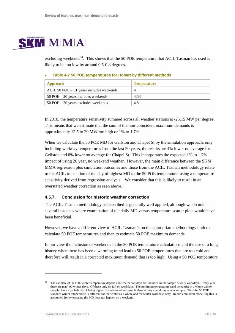
Review of Aurora's maximum demand forecasts
Final report to AER 9 September 2011 PAGE 48
excluding weekends34. This shows that the 50 POE temperature that ACIL Tasman has used is
likely to be too low by around 0.5-0.8 degrees.
Table 4-7 50 POE temperatures for Hobart by different methods
Approach Temperature
ACIL 50 POE – 51 years includes weekends 4
50 POE – 20 years includes weekends 4.53
50 POE – 20 years excludes weekends 4.8
In 2010, the temperature sensitivity summed across all weather stations is -25.15 MW per degree.
This means that we estimate that the sum of the non-coincident maximum demands is
approximately 12.5 to 20 MW too high or 1% to 1.7%.
When we calculate the 50 POE MD for Geilston and Chapel St by the simulation approach, only
including workday temperatures from the last 20 years, the results are 4% lower on average for
Geilston and 8% lower on average for Chapel St. This incorporates the expected 1% to 1.7%
impact of using 20 year, no weekend weather. However, the main difference between the SKM
MMA regression plus simulation outcomes and those from the ACIL Tasman methodology relate
to the ACIL translation of the day of highest MD to the 50 POE temperature, using a temperature
sensitivity derived from regression analysis. We consider that this is likely to result in an
overstated weather correction as seen above.
4.5.7. Conclusion for historic weather correction
The ACIL Tasman methodology as described is generally well applied, although we do note
several instances where examination of the daily MD versus temperature scatter plots would have
been beneficial.
However, we have a different view to ACIL Tasman’s on the appropriate methodology both to
calculate 50 POE temperatures and then to estimate 50 POE maximum demands.
In our view the inclusion of weekends in the 50 POE temperature calculations and the use of a long
history when there has been a warming trend lead to 50 POE temperatures that are too cold and
therefore will result in a corrected maximum demand that is too high. Using a 50 POE temperature
34 The estimate of 50 POE winter temperature depends on whether all days are included in the sample or only workdays. Every year there are (say) 90 winter days. Of these only 64 fall on workdays. The minimum temperature (and demands) in a whole winter sample have a probability of being higher in a whole winter sample than in only a workday winter sample. Thus the 50 POE standard winter temperature is different for the winter as a whole and for winter workdays only. In our simulation modelling this is accounted for by ensuring the MD does not happen on a weekend.

Review of Aurora's maximum demand forecasts
Final report to AER 9 September 2011 PAGE 49
based on only weekdays from the past 20 years will lower the weather corrected MDs calculated by
around 1.5%.
Our main concern is with the methodology used to estimate the 50 POE MD. We consider that the
method used by ACIL Tasman of shifting the actual maximum demand day to the 50 POE
temperature will also lead to overestimated weather corrected MDs in most cases.
When compared to our simulation approach, we estimate that the ACIL weather corrected MDs are
systematically too high by between 4% and 8 %. These are significant differences. We note that a
simulation methodology is also being used by Transgrid in NSW and AEMO for Victoria and
South Australia35. It has also been used in gas demand modelling by AGL in NSW.
ACIL Tasman, in its review of weather correction for Victorian DNSPs has stated:
“The impact that weather has on electricity demand is relevant at both the system and spatial
level. However, weather normalisation at the system level can be undertaken in a more
sophisticated manner than at the spatial level. System level forecasting methodologies are able
to employ more statistically robust procedures which establish a relationship between
maximum demand and temperature using high frequency data (often at 30 minute intervals).
These methodologies allow for a more complex relationship to be established between
temperature and demand (often involving some combination of minimum and maximum
temperatures and lags etc).
The established relationship between demand and some function of temperature may then be
used to simulate a long run probability distribution of demands using a long record (usually in
excess of 50 years) of weather data. The resulting distribution can then be used to establish the
90, 50 and 10 POE levels of demand.
While this approach would be theoretically possible at the spatial level, it is both
computationally and data intensive and thus generally impractical at the spatial level. For this
reason, temperature normalisation or correction at the spatial level usually takes a more
simplistic form. The usual approach is to establish a relationship between the maximum
demand and average temperature for a given season from which specific maximum demands
are derived coinciding with 10 and 50 POE temperatures. The observed maximum demand in a
given year is then adjusted to what would have been observed at the 50 or 10 POE long run
average temperature. In this approach, there is only a one for one relationship between
demand and average temperature.
35 Australian Energy Market Operator (AEMO) Electricity Statement of Opportunities 2011, Page 3-59 available at http://www.aemo.com.au/planning/ESOO2011_CD/documents/chapter3.pdf.

Review of Aurora's maximum demand forecasts
Final report to AER 9 September 2011 PAGE 50
Such an approach is inferior to the simulation based approaches, which allow for more
complex and better fitting relationships between demand and temperature. It is not as
statistically robust because it entails weather correcting or normalising only a single day (i.e.
the day on which the annual maximum occurred) in a given season. Simulation methods on the
other hand construct an entire distribution of maximum demands over a large number of years
from which the 50 and 10 POE maximum demand are obtained.”36
We have discussed our understanding that the weather correction methodology used by ACIL
Tasman may overstate the weather corrections with ACIL Tasman and Aurora at the meeting on 14
July 2011. The response has been that, to the extent there are issues, they are likely to be relatively
minor in relative terms and will, in any case, be largely overcome through the reconciliation
process. While it may be true that the reconciliation will fix the issues and that the relativities
between TS are unlikely to be significantly distorted, we consider that a more appropriate 50 POE
temperature correction will allow the extent of reconciliation required to be better assessed. In
addition, as discussed in Section 4.6 below, the reconciliation itself may be problematic.
While ACIL Tasman has assessed the amount of reconciliation required after weather correction
and trend analysis in each year to be some 1.86% to 3.39% (see Table 4-2), we consider the
required scaling to be significantly higher due to the overstated 50 POE history and forecasts
prepared by ACIL Tasman. For example, this means that the jump to the forecast 2011 of 1152
MW from the 2010 actual of 1022 MW plus an additional (say) 30 MW of weather correction is
very significant, some 100 MW or 9.5%. The reason for such a substantial increase due to the
reconciliation process must be understood.
4.6. Reconciliation to forecast derived from the NIEIR forecasts for Transend
The ACIL Tasman spatial forecasts built from bottom up at TS level are reconciled by Aurora to a
set of externally generated top down global system forecasts which have been derived by Transend
from Tasmania-wide forecasts generated by NIEIR.
Aurora has taken the forecasts provided by Transend and used these numbers as the system MD
numbers. The spatial forecasts derived by ACIL Tasman have been scaled up by from 1.86%-
3.39% each year in order to reconcile with these system forecasts. As we have seen in Section 4.5
above, we believe that these factors actually underestimate the extent of scaling required from 50
POE weather corrected historical and forecasts.
36 ACIL Tasman, “Victorian electricity distribution price review: review of maximum demand forecasts”, final report to Australian Energy Regulator, 19 April 2010, page 5.

Review of Aurora's maximum demand forecasts
Final report to AER 9 September 2011 PAGE 51
4.6.1. Derivation of numbers from NIEIR report to Transend
Each year for at least the past four years Transend has commissioned NIEIR to produce system-
wide forecasts for the Tasmanian transmission network. At Aurora’s request, Transend has
translated the system-wide forecasts produced by NIEIR in 2010 into a component relevant to
Aurora and a component relevant to the dozen or so major industrial customers which are served
directly from the Transend transmission system.
The method used by Transend to achieve this has been described as:
“Until year 2010, diversity factors for the forecast were calculated based on the load at the
connection point, at the time of State maximum demand. The methodology is,
The methodology was also discussed at a meeting between Transend, AER and SKM MMA on
14 July 2011. In addition to the above, methodology the resulting forecasts applicable to Aurora
have been scaled down by a factor of 3.1% to account for transmission losses into the network.
It has been stressed by Transend that the forecasts prepared by NIEIR are those for the transmission
system as a whole and that the distribution network MD may be different to those applicable for the
transmission system as a whole. In addition, we understand that the calculations of distribution
load applicable to Aurora is based on assumptions about constant diversity factors going forward.
While we consider these to be reasonable assumptions from the NIEIR report, this is not the same
as having a purpose developed system forecast for Aurora and it is not clear they measure exactly
the same thing. Thus, for example, looking at the 2005 to 2009 historical information for Aurora
MD provided by Transend to Aurora is consistently different to the actual Aurora system MDs –
higher in some years by up to 8.5% and lower in others by over 4%.
In addition, Transend has stated that in its translations it has used the diversity factors
in its forecasts. As we have discussed in Section 4.3.4, we consider that the
coincidence factors used can make a significant difference and are somewhat concerned that
.
While we do not know what impact this has had it may be material.
37 Email from D Perera of Transend to M Hooper of AER dated 28 July 2011.

Review of Aurora's maximum demand forecasts
Final report to AER 9 September 2011 PAGE 52
As a result, while we consider the method adopted by Transend to translate the NIEIR forecasts
may be reasonable, we have reservations about the use of the NIEIR forecasts for Transend, being
translated and then used directly for system reconciliation by Aurora. We consider that good
practice in reconciliation requires that the histories and key assumptions be agreed and any
discrepancies understood. None of these appears to have been done by Aurora when using the
NIEIR forecasts. In other words, the use of the NIEIR forecasts for Aurora, while certainly
plausible, have not been validated or assessed as being compatible with the Regulatory proposal.
4.6.2. Timeliness and relevance
The NIEIR 2010 forecasts were prepared prior to the 2010 winter and, therefore, forecast for the
year 2010 as well as beyond. The NIEIR forecast applicable to Aurora as derived by Transend
(after the 3.1% losses are applied) was 1128 MW. This is over 100 MW (10%) greater than the
actual Aurora system MD in 2010 which was 1022 MW. Yet Aurora did not attempt to reconcile
the obvious differences between the 2010 forecast and actual MD (only some 30 MW of which was
likely to be due to weather). Instead Aurora used the NIEIR forecast for 2011, presumably
assuming that the additional 100 MW would emerge in 2011 when it did not come in 2010. This
again does not constitute good practice.
We note that for its 2011 forecasts, Transend asked NIEIR to forecast separately for its major
customers and for the remainder (ie Aurora). We have also considered those forecasts in our
overall assessments as they do take into account the winter 2010 results.
4.6.3. Different assumed levels of key drivers
A reconciliation process is important because a global forecast generally allows key drivers which
are not taken into account by the typically mechanical spatial forecasts to be factored into forecasts.
However, the global forecast must be based on the key drivers which the network considers to be
pertinent for the network going forward. It is not reasonable to use global forecasts prepared
externally if the underlying assumptions about key drivers are materially different to those of the
network.
Two of the key drivers of future growth of MD are likely to be economic growth and customer
number growth. In terms of economic growth the assumptions used by NIEIR in its forecasts are
materially different to those of the network and its consultant ACIL Tasman. ACIL Tasman has
assumed a relatively slow economic growth in annual GSP growth rate of 2% between 2010 and
2017 and this appears to be generally consistent with the view taken by Aurora (see Section 3.6).
NIEIR in 2010 assumed a GSP growth rate of about 2.5% pa in its 2010 forecasts and has assumed
a similar rate in its 2011 forecasts.
Similarly, while NIEIR has assumed a customer number growth rate of % pa, the growth
rate assumed by ACIL Tasman is % pa.

Review of Aurora's maximum demand forecasts
Final report to AER 9 September 2011 PAGE 53
4.6.4. NIEIR methodology
Although we have read the NIEIR reports, we have not been able to review the NIEIR
methodology in any detail. As we understand it, NIEIR:
4.6.5. Jump in the initial year
The forecasts derived for Aurora in 2010 and those which appear in the subsequent NIEIR report in
2011 both assume significant growth in the first year of the forecast period followed by a number
38 National Institute of Economic and Industry Research (NIEIR) report to Transend, “Electricity sales and maximum demand forecasts for Tasmania to 2042” May 2011, page 22
39 The same percentile temperatures as in the 2010 report were also used by NIEIR in 2008 and 2009.

Review of Aurora's maximum demand forecasts
Final report to AER 9 September 2011 PAGE 54
of years of much lower growth. Thus, in the 2010 NIEIR report, using winter 2009 data as the
base, NIEIR40 forecast an increase of 96 MW in 2010, followed by an average of 13 MW pa to
2017. The actual recorded MD for Aurora in 2010 was 1022 MW. Although the winter was very
mild, weather correction would be expected to add only of the order of 30 MW to this, with
diversity correction perhaps a further 20 MW.
According to our interpretation of the NIEIR 2011 report, the Aurora system MD would be
expected to increase by 108 MW in 2011 to 1129 MW and then by an average of 17 MW per year
till 2017. However, the interim system MD for Aurora in winter 2011 is below 1000 MW. Again,
the weather correction might be expected to add of the order of 30 MW to this. While the actual
MD recorded in 2011 may well change before the end of winter, we would not expect it to be by of
the order of 130 MW.
The Aurora system MD forecasts as derived from NIEIR reports and actuals (to date for 201141) are
provided in Table 4-8.
Table 4-8 Forecasts for Aurora system MD derived from NIEIR 2010 and 2011 reports to Transend and actual Aurora MD, MW
Transend derived forecast for Aurora 2010, MW
NIEIR 2011 for Transend MD excluding majors,
MW
Actual Aurora MD, MW
2008 1079*1 1092*3 1100*5
2009 1032*1 1047*3 1077*5
2010 1128*2 1021*3 1022*5
2011 1152*2 1129*3 987*6
2012 1159*2 1148*3
2013 1165*2 1163*3
2014 1177*2 1175*3
2015 1189*2 1187*3
2016 1203*2 1209*4
2017 1218*2 1231*4 *1 Sourced from Transend spreadsheet data derived from the NIEIR 2010 report but, on advice, not divided by 1.031 *2 Sourced from Transend spreadsheet data derived from the NIEIR 2010 report and divided by 1.031 *3 Sourced from NIEIR 2011 report Table 5.4 for system MD excluding majors and dividing by 1.031 *4 Sourced from NIEIR 2011 report Table 5.4 for system MD excluding majors and dividing by 1.031 and then interpolating
geometrically between the 2015 and 2019 results to derive values for 2016 and 2017. *5 Sourced from the Aurora RIN addendum 2 MD *6 Advised at meeting on 14 July 2011 that the system MD recorded on 5 July 2011 was 1007 MVA which converts to 987 MW at a
power factor of 0.98.
40 It is actually the translation of NIEIR 2010 system forecasts to Aurora network MD forecasts by Transend, however, we have adopted the shorthand for ease of understanding.
41 We have asked Aurora for daily system MD results but these have not been provided since results for June and for the peak day on 5 July. We note that Transend has stated that its system peak has happened on 5 July for the past 3 years.

Review of Aurora's maximum demand forecasts
Final report to AER 9 September 2011 PAGE 55
The forecast increase by 100 or so MW in the first year of both forecasts appears to be a result of a
return to trend in the modelling. Given recent history, it is by no means clear to us that an increase
of such a magnitude would be expected to eventuate.
4.6.6. Conclusions on use of NIEIR forecasts for Aurora
We have not reviewed in detail the NIEIR forecasting methodology for Transend or its translation
into system MD forecasts for Aurora. We note, however, that NIEIR has been forecasting
maximum demand at Tasmanian system level for Transend for a number of years.
Our main concerns with the use of the NIEIR forecasts by Aurora are that:
They have not been fully reconciled historically to ensure that what is being forecast is
consistent with the Aurora system MD. Indeed, Aurora was not aware of the actual
methodology used by NIEIR. In other words, the NIEIR forecasts have not been validated for
Aurora.
The growth drivers assumed by NIEIR are significantly different to those assumed by Aurora.
The translation of NIEIR forecasts for Aurora in 2010 and 2011 shows a significant jump in
the first year followed by years of moderate growth. Such a jump did not take place in 2010
and, based on evidence to date, is not expected to take place in 2011. As a result, we consider
it likely that the system forecasts derived for Aurora are likely to be over-stated in the first year
and probably to 2017.
Review of Aurora's maximum demand forecasts
Final report to AER 9 September 2011 PAGE 56
5. Aurora’s MD forecasting methodology at feeder level
5.1. RIN forecast methodology
Aurora has provided feeder forecasts in its updated RIN and has produced a spreadsheet which
explains how the feeder forecasts in the RIN were prepared. In essence the methodology was:
Step 1: Collect a data base of feeder maximum demands across the year
Step 2: Filter the MD data to remove spurious results
Step 3: Use the median of the 2007/08, 2008/09 and 2009/10 years as the starting point for
each feeder
Step 4: Grow this starting point uniformly by the UES growth rate for each feeder for of the
years across the period
Step 5: Feeders which either currently exceed the planning rating of 5 MVA or will exceed
that rating according to the forecasts within 5 or 10 years are flagged for investigation,
with a range of potential solutions being considered.
In discussions with Aurora it was stressed that feeders are much more dynamic than substations,
with each potentially having its own profiles and many feeders being subject to load transfers, both
short and longer-term. Aurora has also stressed that its demand forecasting at feeder level and
comparison against feeder capacity rating42 is only used as a flag for investigation of the feeder and
adjacent areas by the planning team in order to confirm there is an issue and then formulate options
and a solution if required.
5.2. Feeder forecast methodology used for capex in the Proposal
Although feeder forecast information was provided in the RIN, during discussions with Aurora we
were advised that the capex forecasts for the Proposal used a starting point of the maximum for the
2008/09 year, rather than the median of the 2007/08, 2008/09 and 2009/10 years. Thus, according
to the discussions, Step 3 above was actually:
Actual Step 3: Use the 2008/09 maximum as the starting point for each feeder
We understand that the other steps were unchanged, including the use of the 2008 UES growth
forecasts.
42 There are a number of feeder ratings that are relevant, including continuous, peak cycling and 1 hour emergency rating. We understand that for 11 kV stations Aurora uses a 5 MVA or 262 Amp flag rating.

Review of Aurora's maximum demand forecasts
Final report to AER 9 September 2011 PAGE 57
Further to this, the AER has asked Aurora to confirm exactly on what basis the feeder capex
forecasts were made.
“Can Aurora please: • confirm which demand forecasts are actually used as the basis for reinforcement capex at feeder, zone substation and terminal substation levels.
• provide the actual demand forecasts used to determine reinforcement capex and capacity constraints for feeders relating to Chapel St and Geilston Bay.”
The response is provided below43.
“For larger projects being undertaken within the current Regulatory Control Period and forecast within the forthcoming Regulatory Control Period, the 2008 UES report was used. These projects include: • St Leonards;
• Howrah;
• Rosny, an initial assessment was undertaken based on the 2008 UES forecast and was subsequently reviewed based upon the 2010 ACIL Tasman forecast;
• Sandford (also referred to as South Arm and Lauderdale). To be reviewed based upon the 2010 ACIL Tasman forecast; and
• Kingston and Blackmans Bay (Kingston updated based upon a review of the project with the 2010 ACIL Tasman forecast). The works associated with feeder augmentations was originally based upon the 2008 UES report. The load forecasts, by station, form the basis of the 2008 Feeder Load Report. The Feeder Load Report was then used as the basis to understand the loading of the system. From this report Aurora conducted preliminary assessment as to the larger issues that either needed to be addressed or that could be managed within the normal suite of activities. These assessments provided the basis for development of the forward expenditure programs. The 2009 UES report was used to develop the 2009 Feeder Load Report. This report was used to reassess works associated with the preliminary analysis for development of the forward expenditure programs. In 2010 a similar process was used with the ACIL Tasman data. The differences between the 2008 and 2009 UES reports were not material enough to affect the outcome of high voltage feeder augmentation projects listed. These reports have been appended as attachments to this Response. The process described above was used to develop Aurora’s forward expenditure program for
reinforcement. This includes the basis for reinforcement capex at feeder, zone and terminal
substations; and capacity constraints for feeders at Chapel Street and Geilston Bay substations.”
As we understand this response, it appears that the 2008 UES report was the basis of all of the
capex forecasts. It appears that these have been reviewed against the UES 2009 report and not
required any material change. Further, we understand that the ACIL Tasman 2010 demand
43 Aurora Energy response to AER/014 part 1 sent by email 26 July 2011.

Review of Aurora's maximum demand forecasts
Final report to AER 9 September 2011 PAGE 58
forecasts have been used in the review of some but not all major projects, but not in reviewing the
feeder projects. The type of review carried out is described below44:
“The methodology applied to evaluate the 2008, 2009 and 2010 forecasts was:
Each station was reviewed and assessed if there significant shifts from the previous forecast
for the areas where work was identified;
Whether those shifts, if significant were understood e.g. permanent load transfers undertaken;
No modelling was used to assess the shifts rather these were undertaken by engineering
analysis / review; and
Two of our engineers assessed the shifts – related it to the proposed program and if there were
no issues then the proposed work was not withheld from the proposal.”
5.3. Review of feeder forecasts for Geilston Bay and Chapel Street
Aurora has provided spreadsheets with the 2008 and 2009 feeder loading reports45. These provide
details about feeders which were “overloaded” at the time, (ie had an MD of 5 MVA) and flagged
those which would, if the growth rate was applied, be overloaded within a five or ten year period.
We have examined the year in which an issue with feeder capacity will be flagged as an indicator
of potential capex in order to relieve a potential capacity constraint. In Table 5-1 we have looked
only at those feeders which might be flagged over the coming regulatory period. These are those
that currently have an MD of 5 MVA or more and those which are forecast to have an MD of 5
MVA or more within the next regulatory period.
In columns 2 to 4, we initially list the MDs by feeder provided in the 2008 and 2009 feeder
loading reports. We then list the 2010 MD provided in the RIN for each of the feeders.
We then list the first year in which feeders would be flagged under the methodologies:
Column 5 uses the 2008 MD plus the UES 2008 growth rates
Column 6 uses the 2009 MD plus the UES 2009 growth rates
Column 7 uses the 2009 MD plus the UES 2008 growth rates. We understand this was the
forecast used initially for the capex forecasts included in the Proposal and have
highlighted this column.
Column 8 uses the RIN forecasts
Column 9 uses the 2010 MDs from the RIN plus the ACIL Tasman growth rates.
It should be noted that if a feeder is “overloaded” in the base year of the forecast then this is
marked “already” in the table. Only if this status changes should attention be paid to these feeders.
44 Email from J Sayers of Aurora to M Hooper of AER dated 29 July 2011. 45 NW-#30056022-v1a_Feeder_Loading_2009.xls and NW-#30008793-v3-2008_Feeder_Loadings.xls

Review of Aurora's maximum demand forecasts
Final report to AER 9 September 2011 PAGE 59
Table 5-1 Feeder maximum demand and year when feeders would be flagged for exceeding 5 MVA for selected feeders in the Chapel Street TS and Geilston Bay ZSS
Feeder 2008 MD, MVA
2009 MD, MVA
2010 MD, MVA
Year flagged 2008, 2008
Year flagged 2009,2009
Year flagged 2009,2008
Year flagged RIN
Year flagged 2010+ACIL
1 2 3 4 5 6 7 8 9
Chapel Street
20535 3.57 4.74 4.4 2011 2012 2014 2011
20541 5.11 5.35 4.6 Already Already Already 2013 2011
20547 7.03 6.31 4.1 Already Already Already 2011
20548 4.98 5.55 5.5 Already Already Already 2011 Already
20549 4.51 4.51 3.6 2012 2013 2014
20552 5.49 5.14 3.3 Already Already Already
Geilston Bay
26162 5.41 5.41 3.0 Already Already Already 2015
26163 4.88 4.88 1.0 2009 2010 2011 2017
26164 4.90 4.90 3.9 2009 2010 2010
26165 5.18 5.14 2.9 Already Already Already 2013
26166 4.57 4.57 3.7 2012 2013 2013
26167 5.66 5.72 4.9 2009 Already Already 2011 2011
26169 4.46 4.31 4.0 2012 2014 2016
For these two stations, it appears that the flagging becomes progressively later using the 2009
actuals and the 2010 actuals. This is understandable, given that the 2009 and 2010 actuals were
generally low, possibly because of mild weather in these years. In addition there is evidence that
some load transfers have already occurred on a number of feeders (see discussion about specific
feeders in Section 5.3).
Using forecasts derived from the 2010 actuals (from the RIN) plus ACIL Tasman growth rates
results in a significant delay in timing of flagging for several feeders in these stations at least.
ssutt
Sticky Note
Unmarked set by ssutt

Review of Aurora's maximum demand forecasts
Final report to AER 9 September 2011 PAGE 60
Although we have seen MD data by feeder for Geilston Bay and Chapel Street, these do not
correspond exactly to the feeder MD data in the spreadsheets from which RIN data have been
derived as provided by Aurora46 .
We provide details about some specific feeders in the sections below.
5.3.1. Some example feeders from Geilston Bay
Feeder data for Geilston Bay Feeder 26165 from several sources provided by Aurora are listed in
Table 5-2 .
Table 5-2 Feeder 26165 information provided by Aurora Energy, MVA
Data Source 2006/07 2007/08 2008/09 2009/10
RIN and Geilston Bay spreadsheet 3.2 5.0 4.7 2.9
Raw max values in Geilston Bay spreadsheet 3.3 5.2 4.7 3.2
Feeder report 2008 5.2
Feeder report 2009 5.14
A graph of the raw data for the feeder from 2003 to 2010, in Amps, is provided in Figure 5-147.
For the feeder calculations each year is defined as being from 1 September to 31 August and the
methodology does not differentiate between maximum demand occurring at different times of the
year.
46 Feeder Max Demand RIN data – Geilston Bay 11 kV.xlsx and Feeder Max Demand RIN data – Chapel St 10f2 11 kV .xlsx and Feeder Max Demand RIN data – Chapel St 20f2 11 kV .xlsx provided by Aurora Energy. For example, for feeder 26162 in Geilston Bay, the RIN data spreadsheet had historical MDs of 5.45 MVA, 4.9 MVA, 4.4 MVA and 3.3 MVA for 2006/07, 2007/08, 2008/09 and 2009/10. The maximum raw data values from which these were derived were 5.7 MVA, 5.41 MVA, 5.35 MVA and 3.3 MVA. The 2008 Feeder Loadings spreadsheet used a feeder loading of 5.41 MVA and the 2009 feeder loading spreadsheet also used a value of 5.41 MVA.
47 It should be noted that for feeders in 11 kV stations (including Geilston Bay and Chapel Street) the conversion between Amps and MVA is 1 MVA = 52.5 Amp. The “flag” for 11 kV substations is 5 MVA or 262 Amp.

Review of Aurora's maximum demand forecasts
Final report to AER 9 September 2011 PAGE 61
Figure 5-1 Feeder Geilston Bay 26165 raw MD in Amps, 2003 to 2010
The early years of the history are as would be expected for what appears to be a reasonably mature
feeder. Apart from a few spurious results, the values appear to increase by a few amps per year.
There is no suggestion that the feeder would approach the 262 Amp limit. However, in the
2008/09 year, from about 23 May 2008 to April 2009, there appears to be a load transfer or a spot
load which increases values by about 100 Amp initially. This additional load is included in the
2008 values and, for a value in September 2008, also in the 2009 MD. The additional load appears
to have been removed in 2009/10, meaning that the feeder appears to have returned to its loading
prior to May 2008.
Returning to the table above, it appears that:
The RIN values have captured slightly lower values than those in the raw data as they carry out
a check for reasonableness which initially moderates apparently anomalous values
The input data for the Feeder reports in 2008 has used the 5.2 MVA value captured on 28 May
2008 for 2007/08 and a value of 4.7 MVA presumably captured on 4 September 2008 for the
2008/09 year.
Despite the MD being flagged in 2008 and 2009, because of the load increase that appears to have
lasted a year or so, based on 2010 actuals there would appear to be no need for a flag for this
feeder. This indicates the need to use the latest possible data for feeder forecasts and to look
carefully at the reason for sudden changes.

Review of Aurora's maximum demand forecasts
Final report to AER 9 September 2011 PAGE 62
We note again that this refers only to the flagging process. We would expect that this would have
been taken into account by the network planners in assessing the need for any augmentation.
Figure 5-2 Feeder Geilston Bay 26162 raw MD in Amps, 2003 to 2010
Feeder 26162 appears to have either lost or transferred some load in 2010. Based on this there
would not expect to be flagged in the next regulatory period. The same appears to be the case for
Feeder 26163 (illustrated) and feeder 26164. Despite an increase of about 8% in the first year, the
growth rate for the station is so low that it appears no flag will be required.

Review of Aurora's maximum demand forecasts
Final report to AER 9 September 2011 PAGE 63
Figure 5-3 Feeder Geilston Bay 26163 raw MD in Amps, 2003 to 2010
Feeder 26167, however, is expected to be flagged (again) in 2011.
Figure 5-4 Feeder Geilston Bay 26167 raw MD in Amps, 2003 to 2010

Review of Aurora's maximum demand forecasts
Final report to AER 9 September 2011 PAGE 64
Thus of the feeders examined from Geilston Bay, when compared against the forecasts using 2009
data and UES 2008 growth rates, almost all flags would have been delayed significantly if the latest
(2010) data and the ACIL Tasman growth forecasts had been used.
5.3.2. Some example feeders from Chapel Street
We provide daily raw data from the Chapel Street feeders which potentially required flagging over
the period in the following figures.
Figure 5-5 Feeder Chapel Street 20535 raw MD in Amps, 2003 to 2010
There appears to have been some load transfer out around 2006 and in around 2009. With the same
load profile a flag would be expected in 2011.
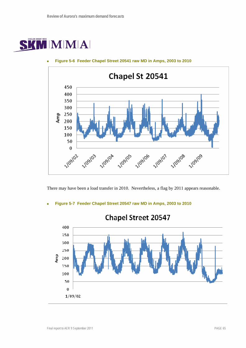
Review of Aurora's maximum demand forecasts
Final report to AER 9 September 2011 PAGE 65
Figure 5-6 Feeder Chapel Street 20541 raw MD in Amps, 2003 to 2010
There may have been a load transfer in 2010. Nevertheless, a flag by 2011 appears reasonable.
Figure 5-7 Feeder Chapel Street 20547 raw MD in Amps, 2003 to 2010

Review of Aurora's maximum demand forecasts
Final report to AER 9 September 2011 PAGE 66
There has clearly been a change in the loading of this feeder in 2010 and no further flag would
appear to be required over the next regulatory period.
Figure 5-8 Feeder Chapel Street 20548 raw MD in Amps, 2003 to 2010
This feeder appears to require flagging from 2010.
Figure 5-9 Feeder Chapel Street 20549 raw MD in Amps, 2003 to 2010

Review of Aurora's maximum demand forecasts
Final report to AER 9 September 2011 PAGE 67
This feeder appears to have undergone changes around 2006 and, despite a couple of high raw
readings does not appear to need to be flagged over the coming regulatory period.
Figure 5-10 Feeder Chapel Street 20552 raw MD in Amps, 2003 to 2010
There appears to have been a change in the load profile of this feeder around 2008 and the feeder
does not appear to need to be flagged within the next regulatory period.
5.3.3. Conclusions from the assessment of feeders in Chapel Street and Geilston Bay
Based on the above analysis and discussion it appears that the flagging of feeders in the Chapel
Street and Geilston Bay stations would have been delayed if the most recent feeder MDs and ACIL
Tasman growth forecasts had been used.
This appears to have been due in part to the more recent MD data being subdued, in part due to
mild weather and in part to changes to feeder load profiles, the reasons for which are not clear from
this analysis.
It appears clear that, for accurate forecasting at feeder level the most recent profiles and growth
rates need to be used.
In terms of methodology, while it would be preferable to correct for load transfers and assess trend
growth at feeder level, as has been done at connection points, this is unlikely to be feasible for
many feeders given the frequent changes that appear to take place. It should, however, be possible

Review of Aurora's maximum demand forecasts
Final report to AER 9 September 2011 PAGE 68
to at least roughly weather correct based on the weather correction for the connection point in
percentage terms, after taking into account any obvious load movements over the past year.
The current approach of assessing feeder MD based on previous years maximum (modified to take
into account spurious results as is currently done) appears appropriate and, without a better
methodology for weather correcting and assessing trends, the use of connection point or substation
growth rates appears reasonable. However, these do need to be the latest available – clearly the
starting points and ACIL Tasman growth rates are quite different to those from the 2009 base and
UES.2008 growth rates. In addition, it is recommended that the winter and summer growth rates
are considered separately, which might alleviate some of the issues seen with Geilston Bay feeder
21565.
In all cases it appears apparent that the historical profiles of feeders need to be examined to
understand what is actually going on – however, we expect that this is already taking place.
In preparing its RIN 6.6 for feeders, Aurora has used as a starting point the median of the
maximum values for 2010, 2009 and 2008 and grown this at the UES 2008 growth rates. While we
understand that this might have been due to the low values observed on many feeders in 2010,
possibly due to mild winter weather, we can see no basis for using a median value. Using a median
value means that any major changes are likely to be lost. We consider it preferable to use the
actual MDs recorded (after inspection to make sure they are relevant and take into account
appropriate changes to the profile of the feeder) and weather correct in percentage terms based on
the connection point correction.
5.4. Consideration at the TS and system levels
While we have seen that for Chapel Street and Geilston Bay feeders the use of the 2009 starting
point and UES growth rates has resulted in feeder flagging at a time materially earlier than would
the use of 2010 MDs and ACIL Tasman growth rates, it is not clear that this would be the case
across all connection points and substations.
In order to evaluate the likely impact at a gross level, we have investigated the differences by
connection points. We have compared the outcome at each connection point from using the TS’s
2009 actual starting values and UES 2008 growth rates (referred to as UES) to 2017, as we
understand to have been used in capex forecasting against the outcome from the ACIL Tasman
forecasts which use more recent starting points and growth rates.
We have compared outcomes at the TS and system levels. The results at TS level are provided in
Table 5-3. The result columns compare actual outcomes in 2017 with “High” meaning that the
UES forecasts are greater in the year 2017 than ACIL forecasts by more than 5%, “Low” meaning
that UES forecasts are less than ACIL Tasman forecasts in 2017 by more than 5% and “OK”
meaning the two outcomes are within ± 5%. The actual ratio of the UES to ACIL Tasman
forecasts is provided under the ratio headings.

Review of Aurora's maximum demand forecasts
Final report to AER 9 September 2011 PAGE 69
Table 5-3 Comparison of forecasts to 2017 of forecasts using 2009 and UES 2008 growth against 2017 outcomes
TS Result* Ratio * TS Result Ratio TS Result Ratio
Gordon High 150% Devonport OK 96% George Town High 128%
Meadowbank High 128% Railton OK 103% Hadspen Low 93%
New Norfolk OK 97% Ulverstone OK 98% Mowbray Low 92%
Tungatinah Low 91% Wesley Vale Low 80% Norwood OK 98%
Waddamana Low 84% Palmerston High 143%
Wayatinah Low 84% Derby Low 82% Trevallyn OK 100%
Scottsdale OK 96%
Avoca High 109% Newton (Henty Gold) Low 94%
St Marys Low 80% Burnie Low 94% Queenstown 22kV OK 100%
Triabunna Low 84% Emu Bay Retail High 112% Rosebery 44kV Low 60%
Port Latta High 123% Rosebery 22kV High 106%
Lindisfarne High 116% Smithton High 119% Savage River High 174%
Rokeby Low 83%
Sorell Low 92%
Bridgewater Low 76%
Chapel St High 108% Electrona Low 76%
Creek Rd High 113% Kermandie High 134%
North Hobart OK 95% Kingston High 111% * Note that the result and ratio are the comparison of 2017 results using the 2009/UES 2008 growth against that using
the ACIL forecasts
Of the 42 Connection Points, only 9 are within ± 5% of each other. Seventeen TSs have UES
forecasts more than 5% higher than ACIL forecasts (including the Chapel Street TS and
Lindisfarne TS which relates to Geilston Bay) while 16 have UES forecasts more than 5% lower
than ACIL forecasts. Clearly there are material differences at a number of TS which may feed into
significant differences in feeder forecasts.
However, at the system level the forecasts produced by using the 2009 actual starting values and
UES growth rates results, by 2017, in a value which is not materially different to the result of the
ACIL Tasman growth forecasts (1331 MW versus 1328 MW) for the sum of the non-coincident
connection points. Overall, the forecast growth rate between 2009 and 2017 is 2.0% pa for both the
UES 2008and the ACIL Tasman reconciled methodology.

Review of Aurora's maximum demand forecasts
Final report to AER 9 September 2011 PAGE 70
Overall, therefore, the growth forecasts we understood were used by Aurora in its capex forecasts
are not dissimilar to those derived by ACIL Tasman. However, the rates at individual TS and
substations might well be expected to be different. While we cannot comment on what this would
mean about capex forecasts at feeder level, it would be worthwhile to compare outlooks for
individual feeders based on the RIN 2010 feeder values grown at the ACIL Tasman growth rates.
However, we have in Section 4.3.4 concluded that the coincidence factors used by ACIL Tasman in
its forecasts are too low and that these should be changed to the average of 3 years or 5 years.
Doing this would be expected to result in a reduction of the sum of the non-coincident MDs by
about 2.5%.in each year.
As a result, this would reduce the ACIL Tasman forecasts in each year and to 1295 MW in 2017
and an annual growth rate of 1.7% pa between 2009 and 2017. This is materially different to the
overall UES 2008 growth rate of 2% pa.
In addition, we consider that the forecasts used by ACIL Tasman are likely to be high because of
the jump in the first year (see Section 4.6). If lower forecasts are used then we would expect the
difference between the forecasts used to generate capex forecasts and the new forecasts to be
correspondingly greater.
A further consideration is the phasing of capital expenditure. While the ACIL Tasman forecasts
show a significant jump from 2010 to 2011, in part due to weather correction but also due to the
reconciliation with NIEIR, and then relatively slow growth thereafter, the UES forecasts assume a
constant growth from 2009 to 2017.

Review of Aurora's maximum demand forecasts
Final report to AER 9 September 2011 PAGE 71
6. Conclusions and recommendations
6.1. Aurora methodology and forecasts at TS level
6.1.1. Approach and methodology
The methodology followed by Aurora in deriving its forecasts at TS level can essentially be broken
down into five key steps:
1. Weather correct the MD history at TS level to 50 POE
2. Derive trend growth rates at TS level based on history corrected for historical load transfers
and block loads and extend these forecasts from the weather corrected starting point taking
into account future load transfers and block loads
3. Use appropriate coincidence factors to derive a “bottom up” coincident forecast derived by
extrapolation of TS growth rates and consideration of new block loads
4. Reconcile this to a top down system forecast prepared externally by scaling each year of
the bottom up forecast to match the top down forecast
5. Use the same coincidence factor as in step 3 to derive the reconciled non-coincident
forecasts at TS level.
While the approach and methodology used by Aurora in deriving its forecasts at TS level is
generally considered to be good practice in outline, we have three significant concerns about its
application. These are in the steps related to weather correction, coincident factor adjustments and
reconciliation.
6.1.2. Weather correction
We believe that the method used by ACIL Tasman to weather correct to 50 POE will overstate the
actual weather corrected maximum demands by a material amount. This is because:
ACIL Tasman has included weekend as well as weekdays in its calculation of 50 POE
temperature, despite stating its expectation that peak demand will occur on weekdays.
The 50 POE temperatures assessed have been based on long-term weather time series.
Because of the warming that has taken place in Tasmania over more recent years we consider
that using the average temperature over the past 20 years is more appropriate.
The method used by ACIL Tasman to derive the 50 POE MD from the temperature on the day
of actual peak demand is likely to produce an inflated weather correction when compared to a

Review of Aurora's maximum demand forecasts
Final report to AER 9 September 2011 PAGE 72
combination of regression and simulation. This is evidenced by ACIL Tasman weather
correcting system MD up by about 60 MW over each of the past three years48, while the
difference between a 50 POE and 90 POE is only of the order of 30 MW or less according to
both SKM MMA 49. We have assessed the degree of over-statement of weather
correction to be some 4% to 8% in the two TS we have reviewed in detail.
ACIL Tasman has argued that, even if its weather correction is over-stated, this would largely be
overcome by the reconciliation process. While we largely agree with this argument, the over-
statement of weather correction in this case tends to understate the amount of reconciliation that
needs to take place. This is especially important when there are uncertainties about the
reconciliation itself.
6.1.3. Coincidence factor adjustment
ACIL Tasman has converted to and from the sum of non-coincident TS historical and forecasts by
using the 2010 coincidence factor. However, this year had an atypically low coincidence factor,
possibly because it was a very mild winter. We consider it more appropriate to have used the
average of the past five years as initially proposed by ACIL Tasman.
This makes a material difference to the outcomes for non-coincident TS as these are calculated by
taking external system coincident forecasts and dividing by the coincidence factors. We have
estimated the difference to be some 2.5% in each year of the next regulatory period. As a result,
we consider that the Aurora non-coincident forecasts are inflated by at least this amount in each
year.
6.1.4. Reconciliation
The ACIL Tasman spatial forecasts built from bottom up at TS level are reconciled by Aurora to a
set of externally generated top down global system forecasts which have been derived by Transend
from Tasmania-wide forecasts generated by NIEIR.
Aurora has taken the forecasts provided by Transend and used these numbers as the system MD
numbers. As a result, the spatial forecasts derived by ACIL Tasman have been scaled up by from
1.86%-3.39% each year in order to reconcile with these system forecasts. As we have seen above,
we believe that these factors actually underestimate significantly the extent of scaling required
from 50 POE weather corrected historical and forecasts.
48 Based on the RIN data, ACIL has weather corrected the system actuals by 63 MW, 57 MW and 73 MW over the past three years. 49 The difference between a 50 POE MD and a 90 POE MD is the difference between an MD that would be expected to be exceeded 1
year in 2 and 9 years in 10. If the difference is 30 MW then the difference between a 50 POE MD and that for a warmer winter peak day, say 95 POE would not be expected to be significantly greater. A weather correction of 60 MW suggested by the ACIL Tasman weather correction methodology is not consistent with a difference of 30 MW between a 50 POE and 90 POE MD.

Review of Aurora's maximum demand forecasts
Final report to AER 9 September 2011 PAGE 73
Although we consider that reconciliation between bottom up spatial forecasts and top down global
forecasts generally represent good practice, we have a number of concerns about the reconciliation
process undertaken by Aurora to forecasts derived from NIEIR including:
The histories have not been fully reconciled historically to ensure that what is being forecast is
consistent with the Aurora system MD. Indeed, Aurora was not aware of the actual
methodology used by NIEIR. In other words, the NIEIR forecasts have not been validated for
Aurora.
The growth drivers assumed by NIEIR are materially different to those assumed by Aurora.
The translation of NIEIR forecasts for Aurora in 2010 and NIEIR forecasts for 2011 show a
significant jump in the first year followed by years of moderate growth. Such a jump did not
take place in 2010 and, based on evidence to date, has also not taken place in 2011.
As a result we consider it likely that the system forecasts derived for Aurora are likely to be over-
stated in the first year and probably through to 2017.
6.2. Aurora methodology and forecasts at feeder level
We understand that a significant proportion of the growth capex proposed for the next regulatory
period relates to high voltage feeders. As a result we have reviewed the growth forecasts at feeder
level. We understand that the capex programs were derived based on 2009 feeder actual MDs
which had been grown at rates from the 2008 UES report. Further, we understand that these
programs were then re-assessed after the UES 2009 and the ACIL Tasman 2010 growth rates
became available and were found to still be applicable.
While we cannot comment on the capex programs, we have assessed that the use of the ACIL
Tasman instead of UES 2008 growth rates would have resulted in materially different growth for
many of the TS including for the Chapel Street and Geilston Bay substations which we have
reviewed in some detail. By comparing outcomes under both the UES 2008 and ACIL Tasman
2010 forecasts we have assessed that, by 2017, out of the 42 TS assessed, the two MD forecasts are
within ±5% of each other for only 9 TS. Seventeen TS have UES forecasts more than 5% higher
than ACIL forecasts (including the Chapel Street TS and Lindisfarne TS which relates to Geilston
Bay) while 16 have UES forecasts more than 5% lower than ACIL forecasts. Clearly there are
significant differences at a number of TS which may feed into significant differences in feeder
forecasts.
At the system level, however, the forecast produced by using the 2009 actual starting values and
UES growth rates results, by 2017, in a value which is not materially different to the result of the
ACIL Tasman growth forecasts (1331 MW versus 1328 MW) for the sum of the non-coincident
connection points. Overall, the forecast growth rate between 2009 and 2017 is 2.0% pa for both the
UES 2008 and the ACIL Tasman reconciled methodology.

Review of Aurora's maximum demand forecasts
Final report to AER 9 September 2011 PAGE 74
However, we have in Section 4.3.4 concluded that the coincidence factors used by ACIL Tasman in
its forecasts are too low and that these should be changed to the average over the past 3 or 5 years.
Doing this would be expected to result in a reduction of the sum of the non-coincident MDs by
about 2.5%.in each year.
As a result, this would reduce the ACIL Tasman forecasts in each year and to 1295 MW in 2017
and an annual growth rate of 1.7% pa between 2009 and 2017. This is materially different to the
overall UES 2008 growth rate of 2% pa.
This amended ACIL Tasman growth rate, combined with the different starting points from feeder
MDs in 2010 as listed in the RIN may result in a different feeder work program at some stations.
We recommend that Aurora be asked to provide feeder forecasts based on the RIN 2010
starting point growing at the ACIL Tasman growth rates amended to take into account a
diversity factor averaged over the past five years.
Even this result may be higher than would be expected to be the case if the global reconciliation
process, about which we have expressed concerns, is considered to be too high, especially in the
first year.
6.3. Trend projection based on data from 2005 to 2011
As discussed in Sections 4.6.5 and 6.3.1, the initial MD results to date for the network in winter
2011 (less than 1000 MW) suggest strongly that the forecast of a coincident system MD of 1152
MW this year is unlikely to eventuate. This is likely to be due to a combination of the initial jump
in 2011 forecast based on reconciliation with the NIEIR forecast for Transend being too steep, and
the economic growth factors assumed by NIEIR under those forecasts and its forecasts for
Transend in 2011 being materially higher than those expected by ACIL Tasman. The difference
between forecast and recent actual MDs are illustrated in Figure 6-1.
If it is confirmed over the entire winter 2011 (that is by end August 2011) that the forecasts in the
first year are indeed significantly too high in the starting year, then we recommend that Aurora be
asked to reconcile to a forecast based on a trend growth line over the past seven years. A
methodology for doing this is described below and compared to the ACIL Tasman and NIEIR 2011
forecasts.
While the use of the aggregated and diversified spatial forecasts prepared by ACIL Tasman without
reconciliation is another possibility, we do not consider this appropriate because of our concerns
about the weather correction undertaken, which we consider to be materially overstated.

Review of Aurora's maximum demand forecasts
Final report to AER 9 September 2011 PAGE 75
6.3.1. A preliminary seven year trend projection for system MD reconciliation
Using the available data for 2011 winter we can estimate the weather corrected MD we would
expect if there is a 50 POE temperature day before the end of winter. Aurora has provided the
history for most days in June 2011 and for the 5th and 7th of July (1007 MVA and 1005 MVA
respectively).
The maximum so far for winter 2011 was 1007 MVA on July 5th. Assuming a power factor of 0.98
means this equates to 987 MW. Including missing Port Latta and Wesley Vale loads (which we
assume are not included, but which assumption remains to be confirmed) raises this to 997 MW.
Using the same simulation methodology employed in Section 4.5.2.3 and the results for the MDs to
date, applying it to the 2011 system level data available so far, we estimate the 2011 50 POE MD
to be about 1028 MW. We expect this to be a reasonable estimate of 50 POE MD for 2011 unless a
new MD is set in later July or August50. However, this cannot be confirmed until the full data for
2011 winter is available after 31 August when a more robust calculation of the 2011 numbers will
be possible.
This figure is around 100 MW lower than either the NIEIR 2010 or 2011 report forecasts. Up to 30
MW of that difference might be explained by the forestry load that may currently not be
operating51.
Based on data in the RIN and the MD estimated for 2011 discussed above, we have prepared a
preliminary seven-year weather corrected and diversity adjusted history and a projection based on
the seven year linear trend.
Figure 6-1 shows the actual coincident system MDs from 2005 to 2010 as orange triangles, SKM
MMA’s weather corrected and diversity corrected values for those years as purple squares and
preliminary estimates of 2011 actual and adjusted MDs as the hollow triangle and blue circle.
We then show a range of forecasts and projections:
The NIEIR 2010 forecast against which Aurora has reconciled and the 2011 NIEIR system
forecast are shown as red and green lines. For reasons discussed above, we consider the
NIEIR forecasts, especially in the early years, to be high.
The 7-year trend of actuals is shown as the orange line. This is likely to be low as there has
been a need for significant weather correction in recent years.
50 We have asked Aurora to provide us with daily system MD data, but none has yet been provided. 51 Aurora has informed us at the meeting on 14 July 2011 that some 20-30 MW of mainly forestry related load (eg the Gunns sawmill
at Triabunna) which would normally be expected to run was not operating at that time. We have asked Aurora to confirm the missing locations and values but have not at this stage, included any additional assumptions about such “missing” load.

Review of Aurora's maximum demand forecasts
Final report to AER 9 September 2011 PAGE 76
A 7-year trend using the weather and diversity adjusted 2011 as a starting point and the linear
growth rate over the past 7 years is illustrated as a dashed purple line52. We note that this
approach is similar to the one used by ACIL Tasman at the TS level.
Finally, a seven year trend of weather and diversity adjusted values starting at the trend value
in 2012 is shown as a solid purple line.
If the system MD for 2011 is indeed found to be of the order of 1000 or so MW, as suggested by
the data to date, then we consider the forecasts derived from NIEIR reports to Transend are likely
to be significantly too high, especially in the early years. In that case we would consider a system
coincident MD derived from a seven year trend projection, as shown with the purple line, to be a
reasonable outcome. Relative to the NIEIR 2010 forecast that Aurora has reconciled to, this
forecast, based on current data, is 5.4% lower in 2011, 4.4% lower in 2012 and 2% lower in 2017.
A linear extrapolation based on 7 years of weather corrected system data would smooth the very
irregular growth seen over the period from 2005 to 2011 and would implicitly assume that growth
over the coming period will be a little slower than that over the period from 2005-2011, as
suggested by the drivers summarised in Section in 3.10.
The resulting projection could then be applied to the ACIL Tasman spatial forecasts as different
reconciliation factors to use to scale the growth at each TS. While we have raised concerns about
the methodology used by ACIL Tasman to carry out its weather correction, we do not consider it
practical within the time available to carry out alternative regression plus simulation weather
corrections and trend projections at each TS.
While we do not agree with the methodology used to weather correct, we do not understand it to
introduce any bias into relative TS forecasts. As a result, we consider a reasonable methodology to
use to evaluate spatial forecasts would be to use the existing Aurora TS forecasts at spatial level,
after incorporating the relatively minor recommended changes to weather data used53, and then
adjust them by the new reconciliation factors from the trend projection.
The resultant TS growth rates could then be applied to 2010 MDs at feeder level as they have been
previously.
52 We have included in this method an assumed 20 MW of missing forestry load. 53 That is, use of a shorter weather history and excluding weekends.

Review of Aurora's maximum demand forecasts
Final report to AER 9 September 2011 PAGE 77
Figure 6-1 System coincident MD History and Forecasts
We recommend that the AER consider such a projection be used for system reconciliation
after the actual MD for winter 2011 are available. If such a projection is adopted then the
feeder forecasts would again need to be reviewed.
900
950
1000
1050
1100
1150
1200
1250
2004 2006 2008 2010 2012 2014 2016 2018
Winter System M
D (MW)
Calendar Year
Co‐incident System MD
Actuals
Weather + Diversity Corrected
2011 Estimate
NIEIR 2010
NIEIR 2011 forecast
7 Year Acutal Trend
7 Year Trend from SKM Weather Corrected
Growth from 2011 Estimate+Forestry
Review of Aurora's maximum demand forecasts
Final report to AER 9 September 2011 PAGE 78
7. Glossary
2012-2017 regulatory control period
The next regulatory period for Aurora from 1 July 2012 to 30 June 2017
ABS Australian Bureau of Statistics
ACIL Tasman or ACIL Consultancy which prepared Aurora’s demand forecasts at Terminal Station level used in the Aurora Regulatory Proposal
Actual or actuals The actual values recorded (as opposed to those which are weather or diversity adjusted)
AEMO Australian Energy Market Operator
AER Australian Energy Regulator
Aurora Energy, Aurora Distribution Network Service Provider for Tasmania
Coincident Happening at the same time. Coincident maximum demand is the maximum demand at a specific level on the network. Coincident network MD is the highest MD recorded for the network in any given year.
CP Connection Point (to the Transend system)
DNSP Distribution Network Service Provider
Global maximum demand Summer or winter coincident maximum demand for the network as a whole. Typically projected on a “top-down” basis based on assessment of key drivers.
GSP Gross State Product – a measure of the goods and services produced in the state in $ terms.
HDD Heating Degree Day measured as the number of degrees C by which the average daily temperature is below 18 C
LT Long-term
Maximum Demand (MD) Single highest measurement of half-hourly average of
Review of Aurora's maximum demand forecasts
Final report to AER 9 September 2011 PAGE 79
instantaneous demand over a period, typically winter or summer.
MVA , MW Measures of electricity demand and maximum demand. MVA (Mega Volt Ampere) is a measure of the “apparent” power or demand. MW or Mega Watt is a measure of the real power or demand. The two measures are required because of the reactive power (MVAR) which is a measure of “losses” due to the effects of capacitance and inductance. MVA and MW are related through the Power Factor (PF).
Native Energy Total energy demand supplied by both scheduled generating units and significant non-scheduled generating units, on a Sent Out basis, over the period.
NEM and NEMMCO National Electricity Market and National Electricity Market Management Company Limited
NER National Electricity Rules
NIEIR National Institute of Economic and Industry Research
Non-coincident MD The MD recorded at a piece of equipment or at a station which may or may not occur at the same time as the MD for the next level of the system or the system as a whole.
Power Factor (PF) The ratio of true power to apparent power in a circuit. PF = MW/MVA.
Probability of Exceedence (POE) MD projections for each season and year are typically represented by a statistical distribution which takes into account key factors such as temperature and day type (e.g. whether a working or non-working day). An MD at a specified POE level is the estimated MD which is likely to be equalled or exceeded at that probability level. For example, a summer MD specified as 10 POE means that the probability of this MD being equalled or exceeded in the summer of that year is estimated to be 10% or 1 year in 10. A 50 POE MD is expected to be equalled or exceeded, on average, 1 year in 2. Distribution network planning by Aurora in Tasmania is typically based on 50 POE forecasts. Note that we often also refer to 50 POE temperatures,

Review of Aurora's maximum demand forecasts
Final report to AER 9 September 2011 PAGE 80
which are the temperatures which would be expected to be exceeded on average one year in two.
Proposal Regulatory Proposals submitted by Aurora to the AER in late May 2011 relating to appropriate revenues and prices for Aurora from 1 July 2012 to 30 June 2017.
RIN Regulatory Information Notice and associated templates containing information
Spatial maximum demand Summer or winter maximum demand for a small part of the network such as a transmission station or zone substation. Typically projected on a “bottom-up” basis based on assessment of recent growth and spot loads.
SWPD Standard weather peak demand
Templates Spreadsheet templates submitted as a response to the RIN in the Proposals.
Transend The transmission network services provider in Tasmania
TS Terminal Station
UES Utility Engineering Solutions who prepared demand forecasts for Aurora in 2008 and 2009
ZSS Zone substation