Review Normal Distribution Statistical...
12
Hypothesis Testing for Proportions 1 HT - 1 Statistical Inference Sampling Distribution 2 Review Normal Distribution Example: Consider the distribution of serum cholesterol levels for 40- to 70-year-old males living in community A has a mean of 211 mg/100 ml, and the standard deviation of 46 mg/100 ml. If an individual is selected from this population, what is the probability that his/her serum cholesterol level is higher than 225? 3 P(X > 225) = ? 225 0 z x 211 X ~ N (m = 211, s = 46) .30 225 - 211 46 = .30 z = .382 .382 4 Statistical Inference 1. Type of Inference: – Estimation – Hypothesis Testing 2. Purpose – Make Decisions about Population Characteristics Population? 5 Statistics Used to Estimate Population Parameters – Sample Mean, – Sample Variance, s 2 – Sample Proportion, … Estimators p ˆ x m population mean s 2 population variance p population proportion Parameters Statistics Theoretical Basis Is Sampling Distribution. 6 Theoretical Probability Distribution of the Sample Statistic. Sampling Distribution What is the Shape of this distribution? What are the values of the parameters such as mean and standard deviation?
Transcript of Review Normal Distribution Statistical...

Hypothesis Testing for Proportions
1
HT - 1
Statistical Inference
Sampling Distribution
2
Review Normal Distribution
Example: Consider the distribution of serum
cholesterol levels for 40- to 70-year-old
males living in community A has a mean of
211 mg/100 ml, and the standard deviation
of 46 mg/100 ml. If an individual is selected
from this population, what is the probability
that his/her serum cholesterol level is higher
than 225?
3
P(X > 225) = ?
225
0
z
x
211
X ~ N (m = 211, s = 46)
.30
225 - 211
46 = .30 z =
.382
.382
4
Statistical Inference
1. Type of Inference:
– Estimation
– Hypothesis Testing
2. Purpose
– Make Decisions
about Population
Characteristics
Population?
5
Statistics Used to Estimate Population Parameters
– Sample Mean,
– Sample Variance, s 2
– Sample Proportion,
…
Estimators
p̂
x m population mean
s 2 population variance
p population proportion
Parameters Statistics
Theoretical Basis Is Sampling Distribution.
6
Theoretical Probability Distribution of the
Sample Statistic.
Sampling Distribution
What is the Shape of this distribution?
What are the values of the parameters
such as mean and standard deviation?

Hypothesis Testing for Proportions
2
7
Sampling Distribution of The
Mean (Normal Theorem) If a random sample is taken from a Normally
distributed population that has a mean m and
a standard deviation s, the sampling
distribution of the sample mean, x, will be
Normal with a mean that is the same as the
population mean, and will have a standard
deviation that is equal to the standard
deviation of the population divided by the
square root of the sample size.
ss
xn
m mx 8
Sampling Distribution of The
Mean (Central Limit Theorem) If a relatively large random sample is taken
from a population that has a mean m and a
standard deviation s, the sampling
distribution of the sample mean, x, will be
approximately a normal distribution with
mean that is the same as the population
mean, and a standard deviation that is equal
to the standard deviation of the population
divided by the square root of the sample
size.
ss
xn
m mx
9
Standard Error of Mean
1. Formula
2. Standard Deviation of the sampling
distribution of the Sample Means,X
3. Less Than Pop. Standard Deviation
n
s
nx
ss
ss
n
10
Sampling Distribution
s = 2
m = 8
x Population
Distribution
m = 8
x
4.025
2xsSampling
Distribution of
Mean for a
sample of size 25
11
Probability Related to Mean
Example: Consider the distribution of serum
cholesterol levels for all 20- to 74-year-old
males living in United States has a mean of
211 mg/100 ml, and the standard deviation
of 46 mg/100 ml. If a random sample of
100 individuals is taken from the population,
what is the probability that the average
serum cholesterol level of these 100
individuals is higher than 225?
12
P(X > 225) = ?
225
3.04
225 - 211
4.6 = 3.04
.001
Cholesterol Level has a mean 211, s.d. 46.
001.0
)04.3()225(
ZPXP
211
n = 100
x
)6.4,211( xxNX sm
0
z

Hypothesis Testing for Proportions
3
Inference on Proportions
HT - 13 HT - 14
Inference on Proportion
Parameter: Population Proportion p (or p)
(Percentage of people has no health insurance)
Statistic: Sample Proportion n
xp ˆ
x is number of successes
n is sample size
Data: 1, 0, 1, 0, 0 4.5
2ˆ p
4.5
00101
x
xp ˆ
HT - 15
Sampling Distribution of
Sample Proportion A random sample of size n from a large population
with proportion of successes (usually represented by a value 1) p , and therefore proportion of failures (usually represented by a value 0) 1 – p , the sampling distribution of sample proportion,
= x/n, where x is the number of successes in the sample, is asymptotically normal with a mean p
and standard deviation . n
pp )1( -
p̂
HT - 16
Sampling Distribution
When sampling from a population that has a
proportion of successes p, the distribution of is approximately normal if n is large,
m = p
n
ppp
)1(ˆ
-s
p̂
p̂
17
Sampling Error
Sample statistic
(point estimate)
ө
Sampling Error = | ө – |
18
Key Elements of
Interval Estimation
Confidence
interval
Sample statistic
(point estimate)
Confidence
limit (lower)
Confidence
limit (upper)
Confidence Level: A probability that the
population parameter falls somewhere
within the interval.
Point estimate Margin of Error
Hypothesis Testing for Proportions
4
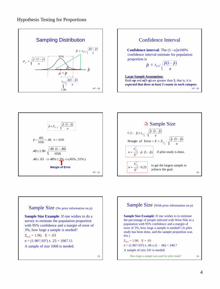
HT - 19
Sampling Distribution
m = p p̂
95%
za/2·
n
pp )ˆ1(ˆ -
1.96
p̂
za/2· n
pp )ˆ1(ˆ -p̂
HT - 20
Confidence Interval
Confidence interval: The (1- a)x100%
confidence interval estimate for population
proportion is
za/2·
n
pp )ˆ1(ˆ -p̂
Large Sample Assumption:
Both np and n(1-p) are greater than 5, that is, it is
expected that there at least 5 counts in each category.
HT - 21
1026 ,481026
495ˆ n.p
)ˆ1(ˆ
ˆ2/
n
ppZp
- a
1026
)48.1(48.96.148.
-
) %51 , %45( %3%48 .03 .48
Margin of Error
22
Sample Size
n
ppp
)ˆ1(ˆzˆ :C.I.
2
- a
n
ppZE
)ˆ1(ˆError ofMargin
2
- a
if pilot study is done. )ˆ1(ˆ2
2
2 ppE
zn -
a
to get the largest sample to
achieve the goal. 25.0
2
2
2 E
zn
a
23
Sample Size (No prior information on p)
Sample Size Example: If one wishes to do a
survey to estimate the population proportion
with 95% confidence and a margin of error of
3%, how large a sample is needed?
Za/2 = 1.96; E = .03
n = (1.962/.032) x .25 = 1067.11
A sample of size 1068 is needed.
24
Sample Size (With prior information on p)
Sample Size Example: If one wishes to to estimate
the percentage of people infected with West Nile in a
population with 95% confidence and a margin of
error of 3%, how large a sample is needed? (A pilot
study has been done, and the sample proportion was
6%.)
Za/2 = 1.96; E = .03
n = (1.962/.032) x .06 x (1 – .06) = 240.7
A sample of size 241 is needed.
How large a sample was used for pilot study?

Hypothesis Testing for Proportions
5
HT - 25
An Alternative Method
nz
nznppznzp
/1
)4/(/)ˆ1(ˆ)2/(ˆ2
2/
22
2/2/
2
2/
a
aaa
-
2//)1(
|/|az
npp
pny
-
-By solving for in p
n
yˆ
The (1- a)x100% Confidence Interval for p is
HT - 26
Hypothesis Testing
1. State research hypotheses or questions.
2. Gather data or evidence (observational or experimental) to answer the question.
3. Summarize data and test the hypothesis.
4. Draw a conclusion.
p = 30% ?
%2525.ˆ p
HT - 27
Statistical Hypothesis
Null hypothesis (H0):
Hypothesis of no difference or no relation,
often has =, , or notation when testing
value of parameters.
Example:
H0: p = 30% or
H0: Percentage of votes for A is 30%. HT - 28
Statistical Hypothesis
Alternative hypothesis (H1 or Ha)
Usually corresponds to research hypothesis and opposite to null hypothesis,
often has >, < or notation in testing mean.
Example:
Ha: p 30% or
Ha: Percentage of votes for A is not 30%.
HT - 29
Hypotheses Statements Example
• A researcher is interested in finding out
whether percentage of people in favor of
policy A is different from 60%.
H0: p = 60%
Ha: p 60%
[Two-tailed test]
HT - 30
Hypotheses Statements Example
• A researcher is interested in finding out
whether percentage of people in a community
that has health insurance is more than 77%.
H0: p = 77% ( or p 77% )
Ha: p > 77%
[Right-tailed test]

Hypothesis Testing for Proportions
6
HT - 31
Hypotheses Statements Example
• A researcher is interested in finding out
whether the percentage of bad product is
less than 10%.
H0: p = 10% ( or p 10% )
Ha: p < 10%
[Left-tailed test]
HT - 32
Evidence
Test Statistic (Evidence): A sample
statistic used to decide whether to reject
the null hypothesis.
HT - 33
Logic Behind
Hypothesis Testing
In testing statistical hypothesis,
the null hypothesis is first assumed to
be true.
We collect evidence to see if the evidence
is strong enough to disprove (reject) the null
hypothesis and therefore support the
alternative hypothesis.
HT - 34
One Sample Z-Test for Proportion
(Large sample test)
Two-Sided Test
HT - 35
I. Hypothesis
One wishes to test whether the percentage
of votes for A is different from 30%
Ho: p = 30% v.s. Ha: p 30%
HT - 36
What will be the key statistic (evidence) to use for testing the hypothesis about population proportion?
Evidence
pSample Proportion:
A random sample of 100 subjects is
chosen and the sample proportion is 25%
or .25.

Hypothesis Testing for Proportions
7
HT - 37
Sampling Distribution
If H0: p = 30% is true, sampling distribution of sample proportion will be approximately normally distributed with mean .3 and standard
deviation (or standard error)
.30
0458.0ˆ ps
0458.0100
)3.1(3.
-
p̂
HT - 38
This implies that the statistic is 1.09 standard
deviations away from the mean .3 under H0 ,
and is to the left of .3 (or less than .3)
09.1
100
)3.1(3.
3.25.
)1(
ˆˆ
00
0
ˆ
0
--
-
-
-
-
n
pp
ppppz
ps
II. Test Statistic
-1.09 0
Z
.25 .30
p̂
HT - 39
Level of Significance
Level of significance for the test (a)
A probability level selected by the
researcher at the beginning of the
analysis that defines unlikely values of
sample statistic if null hypothesis is true.
Total tail area = a
c.v. 0 c.v.
c.v. = critical value
HT - 40
III. Decision Rule Critical value approach: Compare the test statistic
with the critical values defined by significance level a,
usually a = 0.05.
We reject the null hypothesis, if the test statistic
z < –za/2 = –z0.025 = –1.96, or z > za/2 = z0.025 = 1.96.
( i.e., | z | > za/2 )
–1.09
–1.96 0 1.96 Z
a/2=0.025 a/2=0.025
Rejection
region Rejection
region
Two-sided Test
Critical values
HT - 41
III. Decision Rule p-value approach: Compare the probability of the evidence or more extreme evidence to occur when null hypothesis is true. If this probability is less than the level of significance of the test, a, then we reject the null hypothesis. (Reject H0 if p-value < a)
p-value = P(Z -1.09 or Z 1.09) = 2 x P(Z -1.09) = 2 x .1379 = .2758
Z 0
Left tail area .1379
–1.09 Two-sided Test
1.09
Right tail area .138
HT - 42
p-value p-value
The probability of obtaining a test statistic that is as extreme or more extreme than actual sample statistic value given null hypothesis is true. It is a probability that indicates the extremeness of evidence against H0.
The smaller the p-value, the stronger the evidence for supporting Ha and rejecting H0 .

Hypothesis Testing for Proportions
8
HT - 43
IV. Draw conclusion
Since from either
critical value approach z = -1.09 > -za/2= -1.96
or p-value approach p-value = .2758 > a = .05 ,
we do not reject null hypothesis.
Therefore we conclude that there is no
sufficient evidence to support the alternative
hypothesis that the percentage of votes
would be different from 30%.
HT - 44
Steps in Hypothesis Testing
1. State hypotheses: H0 and Ha.
2. Choose a proper test statistic, collect data, checking the assumption and compute the value of the statistic.
3. Make decision rule based on level of significance(a).
4. Draw conclusion. (Reject or not reject null hypothesis)
(Support or not support alternative hypothesis)
HT - 45
When do we use this z-test for
testing the proportion of a
population?
• Large random sample.
HT - 46
One-Sided Test
Example with the same data:
A random sample of 100 subjects is chosen
and the sample proportion is 25% .
HT - 47
I. Hypothesis
One wishes to test whether the percentage
of votes for A is less than 30%
Ho: p = 30% v.s. Ha: p < 30%
HT - 48
What will be the key statistic (evidence) to use for testing the hypothesis about population proportion?
Evidence
pSample Proportion:
A random sample of 100 subjects is
chosen and the sample proportion is 25%
or .25.

Hypothesis Testing for Proportions
9
HT - 49
Sampling Distribution
If H0: p = 30% is true, sampling distribution of sample proportion will be approximately normally distributed with mean .3 and standard
deviation (or standard error)
.30
0458.0ˆ ps
0458.0100
)3.1(3.
-
p̂
HT - 50
This implies that the statistic is 1.09 standard
deviations away from the mean .3 under H0 ,
and is to the left of .3 (or less than .3)
09.1
100
)3.1(3.
3.25.
)1(
ˆˆ
00
0
ˆ
0
--
-
-
-
-
n
pp
ppppz
ps
II. Test Statistic
-1.09 0
Z
.25 .30
p̂
HT - 51
III. Decision Rule Critical value approach: Compare the test statistic
with the critical values defined by significance level a,
usually a = 0.05.
We reject the null hypothesis, if the test statistic
z < –za = –z0.05 = –1.645,
–1.09
–1.645 0 Z
a = .05
Rejection
region
Left-sided Test
HT - 52
III. Decision Rule
p-value approach: Compare the probability of the
evidence or more extreme evidence to occur when
null hypothesis is true. If this probability is less than
the level of significance of the test, a, then we
reject the null hypothesis.
p-value = P(Z -1.09) = P(Z -1.09) = .1379
Z
–1.09 0
Left tail area .1379
Left-sided Test
Z-Table
HT - 53
IV. Draw conclusion
Since from either
critical value approach z = -1.09 > -za/2= -1.645
or p-value approach p-value = .1379 > a = .05 ,
we do not reject null hypothesis.
Therefore we conclude that there is no
sufficient evidence to support the alternative
hypothesis that the percentage of votes is
less than 30%.
HT - 54
Can we see data and then
make hypothesis?
1. Choose a test statistic, collect data, checking the assumption and compute the value of the statistic.
2. State hypotheses: H0 and HA.
3. Make decision rule based on level of significance(a).
4. Draw conclusion. (Reject null hypothesis or not)

Hypothesis Testing for Proportions
10
HT - 55
Errors in Hypothesis Testing
Possible statistical errors:
• Type I error: The null hypothesis is true,
but we reject it.
• Type II error: The null hypothesis is false,
but we don’t reject it.
Z p
a
“a” is the probability of committing Type I Error.
HT - 56
One-Sample z-test for a
population proportion
z-test:
Step 1: State Hypotheses (choose one of the three
hypotheses below)
i) H0 : p = p0 v.s. HA : p p0 (Two-sided test)
ii) H0 : p = p0 v.s. HA : p > p0 (Right-sided test)
iii) H0 : p = p0 v.s. HA : p < p0 (Left-sided test)
HT - 57
Test Statistic
Step 2: Compute z test statistic:
n
pp
ppz
)1(
ˆ
00
0
-
-
HT - 58
Step 3: Decision Rule:
p-value approach: Compute p-value,
if HA : p p0 , p-value = 2·P( Z | z | )
if HA : p > p0 , p-value = P( Z z )
if HA : p < p0 , p-value = P( Z z )
reject H0 if p-value < a
Critical value approach: Determine critical value(s) using a , reject H0 against
i) HA : p p0 , if | z | > za/2
ii) HA : p > p0 , if z > za
iii) HA : p < p0 , if z < - za
Step 4: Draw Conclusion.
HT - 59
Example: A researcher hypothesized that the
percentage of the people living in a community
who has no insurance coverage during the past
12 months is not 10%. In his study, 1000
individuals from the community were randomly
surveyed and checked whether they were
covered by any health insurance during the 12
months. Among them, 122 answered that they
did not have any health insurance coverage
during the last 12 months. Test the researcher’s
hypothesis at the level of significance of 0.05.
HT - 60
Hypothesis: H0 : p = .10 v.s. HA : p .10 (Two-sided test)
32.2
1000
)10.1(10.
10.122.
)1(
ˆ
00
0 -
-
-
-
n
pp
ppz
Test Statistic:
p-value = 2 x .0102 = .0204
Decision Rule: Reject null hypothesis if p-value < .05.
Conclusion: p-value = .0204 < .05. There is sufficient
evidence to support the alternative hypothesis that the
percentage is statistically significantly different from 10%.
Ex. 8.10

Hypothesis Testing for Proportions
11
Binomial Test
HT - 61
32.2
1000
)10.1(10.
10.122.
)1(
ˆ
00
0 -
-
-
-
n
pp
ppzZ-Test Statistic:
P(Z >2.32) = 0.0102, p-value = 2 x .0102 = .0204
Binomial Test: test statistic = 122
(Exact Test)
P(Xb 122 | p = .1) = 0.0134, p-value = 2 x .0134 = .0268
HT - 62
Purpose: Compare proportions of two populations
Assumption: Two independent large random samples.
Step 1: Hypothesis:
1) H0: p1 = p2 v.s. HA: p1 p2
2) H0: p1 = p2 v.s. HA: p1 > p2
3) H0: p1 = p2 v.s. HA: p1 < p2
Two Independent Samples z-test
for Two Proportions
HT - 63
Step 2: Test Statistic:
-
---
21
2121
111
nnpp
ppppz
)ˆ(ˆ
)(ˆˆ
1
1
1n
xp ˆ
2
2
2n
xp ˆ
21
21
nn
xxp
ˆ
If a random sample of size n1 from population 1 has x1 successes,
and a random sample of size n2 from population 2 has x2
successes, the sample proportions of these two samples are
(proportion of successes in sample 1)
(proportion of successes in sample 2)
(overall sample proportion of successes)
(If H0: p1 = p2 , then p1 – p2 = 0 )
z has a standard normal distribution if n 1 and n 2 are large. HT - 64
Step 3: Decision Rule:
p-value approach: Compute p-value,
if HA : p1 p2 , p-value = 2·P( Z | z | )
if HA : p1 > p2 , p-value = P( Z z )
if HA : p1 < p2 , p-value = P( Z z )
reject H0 if p-value < a
Critical value approach: Determine critical value(s) using a ,
reject H0 against
i) HA : p1 p2 if | z | > za/2
ii) HA : p1 > p2 if z > za
iii) HA : p1 < p2 if z < - za
Step 4: Conclusion
HT - 65
Example: Test to see if the percentage of
smokers in country A is significant different from
country B, at 5% level of significance?
For country A, 1500 adults were randomly
selected and 551 of them were smokers.
For country B, 2000 adults were randomly
selected and 652 of them were smokers.
1p̂
2p̂
p̂
= 551/1500 = .367 (Country A)
= 652/2000 = .326 (Country B)
=(551+652)/(1500+2000) =.344
(overall percentage of smokers)
HT - 66
Step 1:
Hypothesis:
H0: p1 = p2 v.s. HA: p1 p2
532
2000
1
1500
13441344
0326367.
).(.
..
-
--z
Step 2:
Test Statistic:
p-value = .0057x2 = 0.0114
Hypothesis Testing for Proportions
12
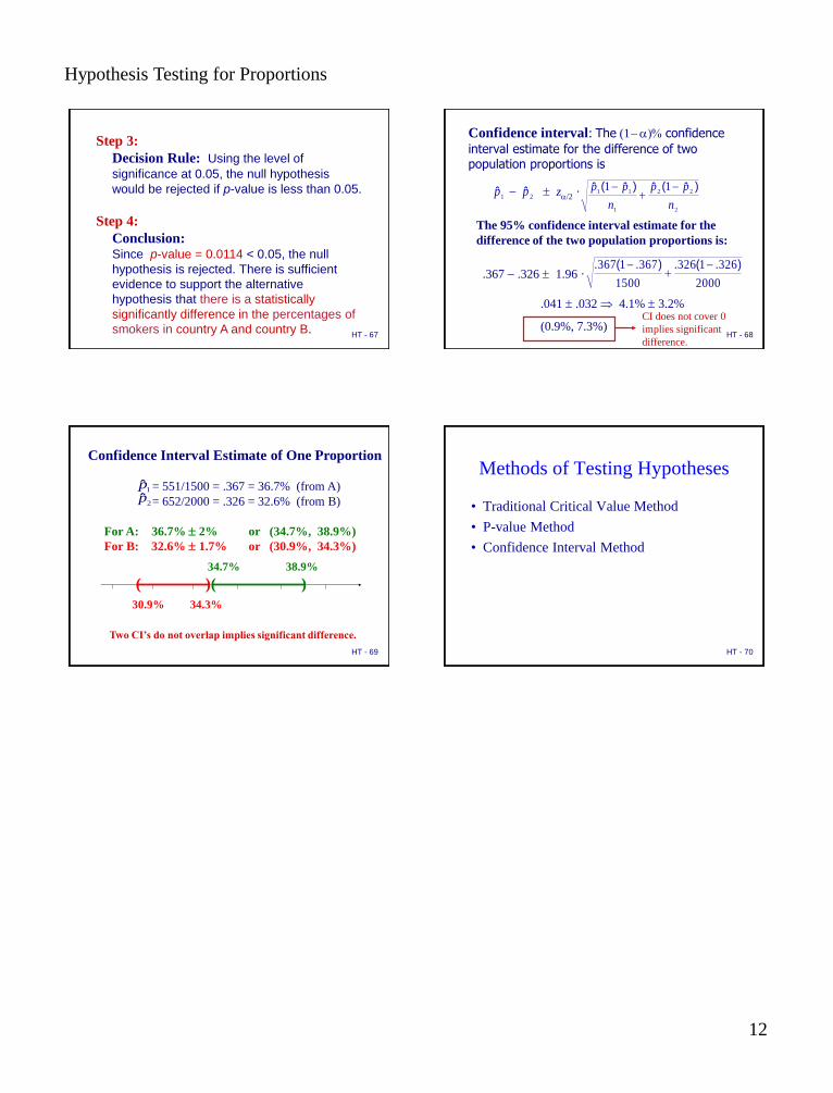
HT - 67
Step 3:
Decision Rule: Using the level of
significance at 0.05, the null hypothesis
would be rejected if p-value is less than 0.05.
Step 4:
Conclusion: Since p-value = 0.0114 < 0.05, the null
hypothesis is rejected. There is sufficient
evidence to support the alternative
hypothesis that there is a statistically
significantly difference in the percentages of
smokers in country A and country B. HT - 68
Confidence interval: The (1- a)% confidence
interval estimate for the difference of two population proportions is
za/2 · 21
pp ˆˆ -
2
22
1
1111
n
pp
n
pp )ˆ(ˆ)ˆ(ˆ -
-
2000
3261326
1500
3671367 ).(.).(. -
-
The 95% confidence interval estimate for the
difference of the two population proportions is:
.367 - .326 1.96 ·
.041 .032 4.1% 3.2%
(0.9%, 7.3%) CI does not cover 0
implies significant
difference.
HT - 69
34.7% 38.9%
( )( )
30.9% 34.3%
Confidence Interval Estimate of One Proportion
= 551/1500 = .367 = 36.7% (from A)
= 652/2000 = .326 = 32.6% (from B)
For A: 36.7% 2% or (34.7%, 38.9%)
For B: 32.6% 1.7% or (30.9%, 34.3%)
1p̂
2p̂
Two CI’s do not overlap implies significant difference.
HT - 70
Methods of Testing Hypotheses
• Traditional Critical Value Method
• P-value Method
• Confidence Interval Method