Review for Exam 3. Triple integral in spherical...
24
Review for Exam 3. Sections 15.1-15.4, 15.6. 50 minutes. 5 problems, similar to homework problems. No calculators, no notes, no books, no phones. No green book needed. Triple integral in spherical coordinates (Sect. 15.6). Example Use spherical coordinates to find the volume of the region outside the sphere ρ = 2 cos(φ) and inside the half sphere ρ = 2 with φ ∈ [0,π/2]. Solution: First sketch the integration region. ρ = 2 cos(φ) is a sphere, since ρ 2 =2ρ cos(φ) ⇔ x 2 + y 2 + z 2 =2z x 2 + y 2 +(z - 1) 2 =1. ρ = 2 is a sphere radius 2 and φ ∈ [0,π/2] says we only consider the upper half of the sphere. rho = 2 cos ( 0 ) y z x 1 2 2 2 rho = 2
Transcript of Review for Exam 3. Triple integral in spherical...
Review for Exam 3.
I Sections 15.1-15.4, 15.6.
I 50 minutes.
I 5 problems, similar to homework problems.
I No calculators, no notes, no books, no phones.
I No green book needed.
Triple integral in spherical coordinates (Sect. 15.6).
Example
Use spherical coordinates to find the volume of the region outsidethe sphere ρ = 2 cos(φ) and inside the half sphere ρ = 2 withφ ∈ [0, π/2].
Solution: First sketch the integration region.
I ρ = 2 cos(φ) is a sphere, since
ρ2 = 2ρ cos(φ) ⇔ x2+y2+z2 = 2z
x2 + y2 + (z − 1)2 = 1.
I ρ = 2 is a sphere radius 2 andφ ∈ [0, π/2] says we only considerthe upper half of the sphere.
rho = 2 cos ( 0 )
y
z
x
1
2
2
2
rho = 2
Triple integral in spherical coordinates (Sect. 15.6).
Example
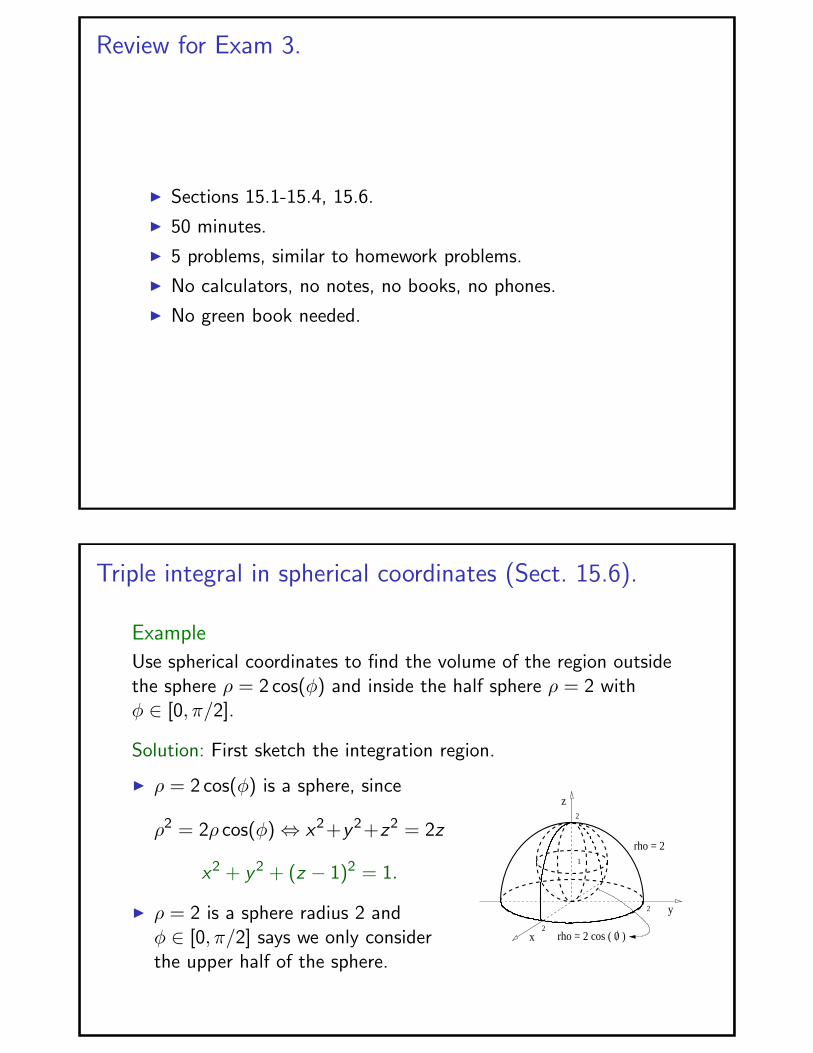
Use spherical coordinates to find the volume of the region outsidethe sphere ρ = 2 cos(φ) and inside the sphere ρ = 2 withφ ∈ [0, π/2].
Solution:
rho = 2 cos ( 0 )
y
z
x
1
2
2
2
rho = 2
V =
∫ 2π
0
∫ π/2
0
∫ 2
2 cos(φ)ρ2 sin(φ) dρ dφ dθ.
V = 2π
∫ π/2
0
(ρ3
3
∣∣∣22 cos(φ)
)sin(φ) dφ
=2π
3
∫ π/2
0
[8 sin(φ)− 8 cos3(φ) sin(φ)
]dφ.
V =16π
3
[(− cos(φ)
∣∣∣π/2
0
)−
∫ π/2
0cos3(φ) sin(φ) dφ
].
Triple integral in spherical coordinates (Sect. 15.6).
Example
Use spherical coordinates to find the volume of the region outsidethe sphere ρ = 2 cos(φ) and inside the sphere ρ = 2 withφ ∈ [0, π/2].
Solution: V =16π
3
[(− cos(φ)
∣∣∣π/2
0
)−
∫ π/2
0cos3(φ) sin(φ) dφ
].
Introduce the substitution: u = cos(φ), du = − sin(φ) dφ.
V =16π
3
[1 +
∫ 0
1u3 du
]=
16π
3
[1 +
(u4
4
∣∣∣01
)]=
16π
3
(1− 1
4
).
V =16π
3
3
4⇒ V = 4π.
C
Triple integral in cylindrical coordinates (Sect. 15.6).
Example
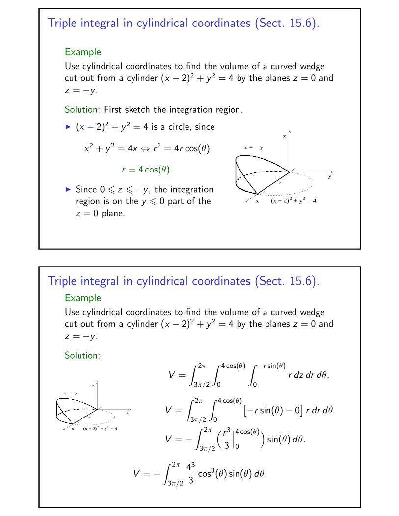
Use cylindrical coordinates to find the volume of a curved wedgecut out from a cylinder (x − 2)2 + y2 = 4 by the planes z = 0 andz = −y .
Solution: First sketch the integration region.
I (x − 2)2 + y2 = 4 is a circle, since
x2 + y2 = 4x ⇔ r2 = 4r cos(θ)
r = 4 cos(θ).
I Since 0 6 z 6 −y , the integrationregion is on the y 6 0 part of thez = 0 plane.
4
x
y
z
z = − y
2
2
(x − 2) + y = 42
Triple integral in cylindrical coordinates (Sect. 15.6).
Example
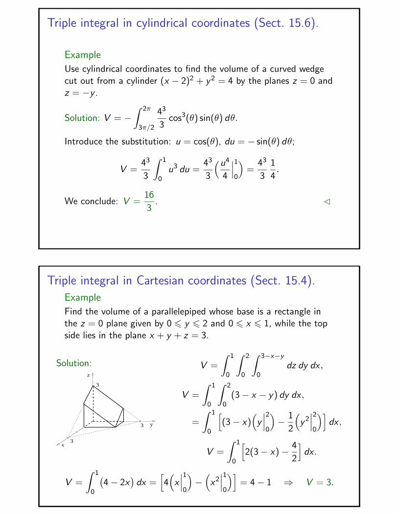
Use cylindrical coordinates to find the volume of a curved wedgecut out from a cylinder (x − 2)2 + y2 = 4 by the planes z = 0 andz = −y .
Solution:
4
x
y
z
z = − y
2
2
(x − 2) + y = 42
V =
∫ 2π
3π/2
∫ 4 cos(θ)
0
∫ −r sin(θ)
0r dz dr dθ.
V =
∫ 2π
3π/2
∫ 4 cos(θ)
0
[−r sin(θ)− 0
]r dr dθ
V = −∫ 2π
3π/2
( r3
3
∣∣∣4 cos(θ)
0
)sin(θ) dθ.
V = −∫ 2π
3π/2
43
3cos3(θ) sin(θ) dθ.
Triple integral in cylindrical coordinates (Sect. 15.6).
Example
Use cylindrical coordinates to find the volume of a curved wedgecut out from a cylinder (x − 2)2 + y2 = 4 by the planes z = 0 andz = −y .
Solution: V = −∫ 2π
3π/2
43
3cos3(θ) sin(θ) dθ.
Introduce the substitution: u = cos(θ), du = − sin(θ) dθ;
V =43
3
∫ 1
0u3 du =
43
3
(u4
4
∣∣∣10
)=
43
3
1
4.
We conclude: V =16
3. C
Triple integral in Cartesian coordinates (Sect. 15.4).
Example
Find the volume of a parallelepiped whose base is a rectangle inthe z = 0 plane given by 0 6 y 6 2 and 0 6 x 6 1, while the topside lies in the plane x + y + z = 3.
Solution:z
x3
y3
3
V =
∫ 1
0
∫ 2
0
∫ 3−x−y
0dz dy dx ,
V =
∫ 1
0
∫ 2
0(3− x − y) dy dx ,
=
∫ 1
0
[(3− x)
(y∣∣∣20
)− 1
2
(y2
∣∣∣20
)]dx ,
V =
∫ 1
0
[2(3− x)− 4
2
]dx .
V =
∫ 1
0
(4− 2x
)dx =
[4(x∣∣∣10
)−
(x2
∣∣∣10
)]= 4− 1 ⇒ V = 3.
Double integrals in polar coordinates. (Sect. 15.3)
Example
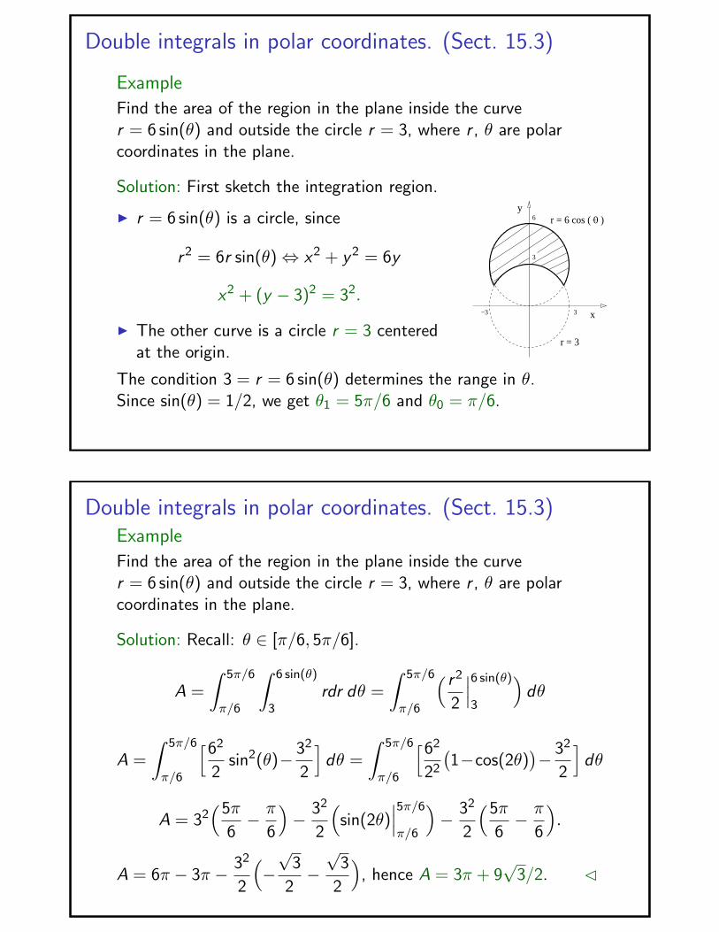
Find the area of the region in the plane inside the curver = 6 sin(θ) and outside the circle r = 3, where r , θ are polarcoordinates in the plane.
Solution: First sketch the integration region.
I r = 6 sin(θ) is a circle, since
r2 = 6r sin(θ) ⇔ x2 + y2 = 6y
x2 + (y − 3)2 = 32.
I The other curve is a circle r = 3 centeredat the origin.
r = 3
x
y
3
3−3
6 r = 6 cos ( 0 )
The condition 3 = r = 6 sin(θ) determines the range in θ.Since sin(θ) = 1/2, we get θ1 = 5π/6 and θ0 = π/6.
Double integrals in polar coordinates. (Sect. 15.3)Example
Find the area of the region in the plane inside the curver = 6 sin(θ) and outside the circle r = 3, where r , θ are polarcoordinates in the plane.
Solution: Recall: θ ∈ [π/6, 5π/6].
A =
∫ 5π/6
π/6
∫ 6 sin(θ)
3rdr dθ =
∫ 5π/6
π/6
( r2
2
∣∣∣6 sin(θ)
3
)dθ
A =
∫ 5π/6
π/6
[62
2sin2(θ)− 32
2
]dθ =
∫ 5π/6
π/6
[62
22
(1−cos(2θ)
)− 32
2
]dθ
A = 32(5π
6− π
6
)− 32
2
(sin(2θ)
∣∣∣5π/6
π/6
)− 32
2
(5π
6− π
6
).
A = 6π − 3π − 32
2
(−√
3
2−√
3
2
), hence A = 3π + 9
√3/2. C
Double integrals in Cartesian coordinates. (Sect. 15.2)
Example
Find the y -component of the centroid vector in Cartesiancoordinates in the plane of the region given by the diskx2 + y2 6 9 minus the first quadrant.
Solution: First sketch the integration region.
3
y
x3
y =1
A
∫∫R
y dA, where A = πR2(3/4), with
R = 3. That is, A = 27π/4. We use polarcoordinates to compute y .
y =4
27π
∫ 2π
π/2
∫ 3
0r sin(θ) rdr dθ.
y =4
27π
(− cos(θ)
∣∣∣2π
π/2
)( r3
3
∣∣∣30
)=
4
27π(−1)(9) ⇒ y = − 4
3π.
Double integrals in polar coordinates. (Sect. 15.2)
Example
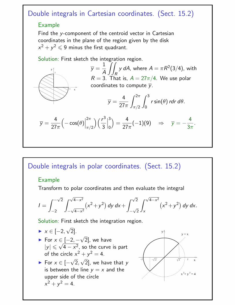
Transform to polar coordinates and then evaluate the integral
I =
∫ −√
2
−2
∫ √4−x2
−√
4−x2
(x2+y2
)dy dx +
∫ √2
−√
2
∫ √4−x2
x
(x2+y2
)dy dx .
Solution: First sketch the integration region.
I x ∈ [−2,√
2].
I For x ∈ [−2,−√
2], we have|y | 6
√4− x2, so the curve is part
of the circle x2 + y2 = 4.
I For x ∈ [−√
2,√
2], we have that yis between the line y = x and theupper side of the circlex2 + y2 = 4.
2
y
x
x + y = 4
y = x
2−2 2− 2
2
Double integrals in polar coordinates. (Sect. 15.2)
Example
Transform to polar coordinates and then evaluate the integral
I =
∫ −√
2
−2
∫ √4−x2
−√
4−x2
(x2+y2
)dy dx +
∫ √2
−√
2
∫ √4−x2
x
(x2+y2
)dy dx .
Solution:
2
y
x
x + y = 4
y = x
2−2 2− 2
2
I =
∫ 5π/4
π/4
∫ 2
0r2 rdr dθ
I =(5π
4− π
4
) ∫ 2
0r3 dr
I = π( r4
4
∣∣∣20
)We conclude: I = 4π. C
Double integrals in polar coordinates. (Sect. 15.2)
Example
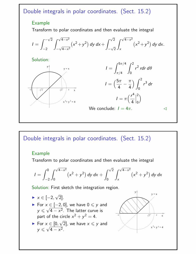
Transform to polar coordinates and then evaluate the integral
I =
∫ 0
−2
∫ √4−x2
0
(x2 + y2
)dy dx +
∫ √2
0
∫ √4−x2
x
(x2 + y2
)dy dx
Solution: First sketch the integration region.
I x ∈ [−2,√
2].
I For x ∈ [−2, 0], we have 0 6 y andy 6
√4− x2. The latter curve is
part of the circle x2 + y2 = 4.
I For x ∈ [0,√
2], we have x 6 y andy 6
√4− x2.
2
y
x
x + y = 4
y = x
2−2 2
2
Double integrals in polar coordinates. (Sect. 15.2)
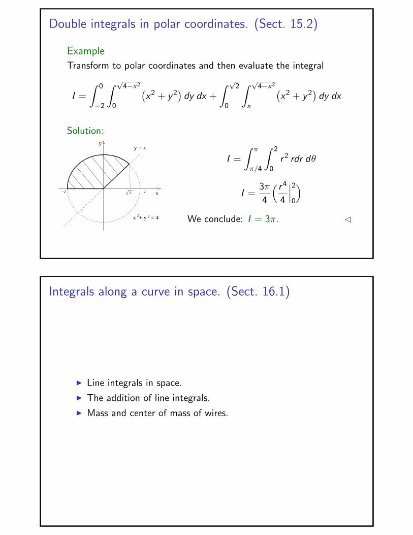
Example
Transform to polar coordinates and then evaluate the integral
I =
∫ 0
−2
∫ √4−x2
0
(x2 + y2
)dy dx +
∫ √2
0
∫ √4−x2
x
(x2 + y2
)dy dx
Solution:
2
y
x
x + y = 4
y = x
2−2 2
2
I =
∫ π
π/4
∫ 2
0r2 rdr dθ
I =3π
4
( r4
4
∣∣∣20
)We conclude: I = 3π. C
Integrals along a curve in space. (Sect. 16.1)
I Line integrals in space.
I The addition of line integrals.
I Mass and center of mass of wires.
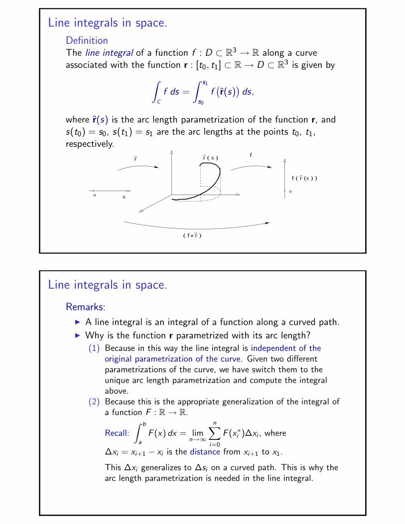
Line integrals in space.
DefinitionThe line integral of a function f : D ⊂ R3 → R along a curveassociated with the function r : [t0, t1] ⊂ R → D ⊂ R3 is given by∫
C
f ds =
∫ s1
s0
f(r(s)
)ds,
where r(s) is the arc length parametrization of the function r, ands(t0) = s0, s(t1) = s1 are the arc lengths at the points t0, t1,respectively.
( f r )
r ( s )rf
f ( r (s ) )
s00
Line integrals in space.
Remarks:
I A line integral is an integral of a function along a curved path.I Why is the function r parametrized with its arc length?
(1) Because in this way the line integral is independent of theoriginal parametrization of the curve. Given two differentparametrizations of the curve, we have switch them to theunique arc length parametrization and compute the integralabove.
(2) Because this is the appropriate generalization of the integral ofa function F : R → R.
Recall:
∫ b
a
F (x) dx = limn→∞
n∑i=0
F (x∗i )∆xi , where
∆xi = xi+1 − xi is the distance from xi+1 to x1.
This ∆xi generalizes to ∆si on a curved path. This is why thearc length parametrization is needed in the line integral.
Line integrals in space.
Theorem (Arbitrary parametrization.)
The line integral of a continuous function f : D ⊂ R3 → R along adifferentiable curve r : [t0, t1] ⊂ R → D ⊂ R3 is given by∫
C
f ds =
∫ t1
t0
f (r(t)) |r′(t)| dt,
where t is any parametrization of the vector-valued function r.
Proof: The integration by substitution formula says∫ s1
s0
f(r(s)
)ds =
∫ t1
t0
f[r(s(t))
]s ′(t) dt,
s0 = s(t0),
s1 = s(t1).
The arc length function is s(t) =∫ tt0|r′(τ)| dτ , then s ′(t) = |r′(t)|.
Noticing that r(s(t)) = r(t), then∫C
f ds =
∫ s1
s0
f(r(s)
)ds =
∫ t1
t0
f (r(t)) |r′(t)| dt.
Line integrals in space.
Example
Evaluate the line integral of the function f (x , y , z) = xy + y + zalong the curve r(t) = 〈2t, t, 2− 2t〉 in the interval t ∈ [0, 1].
Solution: Recall:
∫C
f ds =
∫ t1
t0
f (r(t)) |r′(t)| dt.
The derivative vector is r′(t) = 〈2, 1,−2〉, therefore its magnitudeis |r′(t)| =
√4 + 1 + 4 = 3. The values of f along the curve are
f (r(t)) = (2t)t + t + (2− 2t) ⇒ f (r(t)) = 2t2 − t + 2.∫C
f ds =
∫ 1
0(2t2 − t + 2) 3 dt = 3
[(2t3
3− t2
2+ 2t
)∣∣∣10
].
∫C
f ds = 3(2
3− 1
2+ 2
)= 2− 3
2+ 6 ⇒
∫C
f ds =13
2. C
Line integrals in space.
Example
Evaluate the line integral of the function f (x , y , z) =√
x2 + z2
along the curve r(t) = 〈0, a cos(t), a sin(t)〉, in t ∈ [0, π/2].
Solution: Recall:
∫C
f ds =
∫ t1
t0
f (r(t)) |r′(t)| dt.
The derivative vector is r′(t) = 〈0,−a sin(t), a cos(t)〉, therefore its
magnitude is |r′(t)| =√
a2 sin2(t) + a2 cos2(t) = |a|. The valuesof f along the curve are
f (r(t)) =
√0 + a2 sin2(t) ⇒ f (r(t)) = |a|| sin(t)|.∫
C
f ds =
∫ π/2
0|a| sin(t) |a| dt = a2
(− cos(t)
∣∣∣π/2
0
).
∫C
f ds = a2. C
Integrals along a curve in space. (Sect. 16.1)
I Line integrals in space.
I The addition of line integrals.
I Mass and center of mass of wires.
The addition of line integrals.
TheoremIf a curve C ⊂ D in space is the union of the differentiable curvesC1, · · · , Cn, then the line integral of a continuous functionf : D ⊂ R3 → R along C satisfies∫
C
f ds =
∫C1
f ds + · · ·+∫
Cn
f ds.
Remark:This result is useful to compute lineintegral along piecewise differentiablecurves.
2z
C
x
y
2
C 1
C = C U C1
The addition of line integrals.Example
Evaluate the line integral of f (x , y , z) = x +√
y − z2 along thepath C = C1 ∪ C2, where C1 is the image of r1(t) = 〈t, t2, 0〉 fort ∈ [0, 1], and C2 is the image of r2(t) = 〈1, 1, t〉 for t ∈ [0, 1].
Solution:
C
z
2
1
1
x
yC 1
∫C
f ds =
∫C1
f ds +
∫C2
f ds.
r′1(t) = 〈1, 2t, 0〉 ⇒ |r′1(t)| =√
1 + 4t2.
f (r1(t)) = t + t = 2t.∫C1
f ds =
∫ 1
02t
√1 + 4t2 dt, u = 1 + 4t2, du = 8t dt.
∫C1
f ds =1
4
∫ 5
1u1/2 du =
1
4
2
3
(u3/2
∣∣∣51
)⇒
∫C1
f ds =1
6(5√
5− 1).
The addition of line integrals.Example
Evaluate the line integral of f (x , y , z) = x +√
y − z2 along thepath C = C1 ∪ C2, where C1 is the image of r1(t) = 〈t, t2, 0〉 fort ∈ [0, 1], and C2 is the image of r2(t) = 〈1, 1, t〉 for t ∈ [0, 1].
Solution:
C
z
2
1
1
x
yC 1
∫C
f ds =
∫C1
f ds +
∫C2
f ds.
r′2(t) = 〈0, 0, 1〉 ⇒ |r′2(t)| = 1.
f (r2(t)) = 1 + 1− t2 = 2− t2.
∫C2
f ds =
∫ 1
0(2− t2) dt = 2
(t∣∣∣10
)−
( t3
3
∣∣∣10
)= 2− 1
3=
5
3.∫
C
f ds =1
6(5√
5− 1) +5
3⇒
∫C1
f ds =1
6(5√
5 + 9). C
Integrals along a curve in space. (Sect. 16.1)
I Line integrals in space.
I The addition of line integrals.
I Mass and center of mass of wires.
Mass and center of mass of wires.
Remark:The total mass, the center of mass, and the moments of inertia ofwires with arbitrary shapes in space, given by a curve C and havinga density function ρ, can be computed using line integrals.
I M =∫
Cρ ds;
I x =1
M
∫C
xρ ds, y =1
M
∫C
yρ ds, z =1
M
∫C
zρ ds;
I Ix =1
M
∫C
(y2 + z2)ρ ds,
I Iy =1
M
∫C
(x2 + z2)ρ ds,
I Iz =1
M
∫C
(x2 + y2)ρ ds.
Mass and center of mass of wires.
Example
Find the moments of inertia of a wheel of radius R and density ρ0.
Solution: We place the wheel at the center of the z = 0 plane. Thecurve for the wheel is r(t) = 〈R cos(t),R sin(t), 0〉, t ∈ [0, 2π].Therefore, r′(t) = 〈−R sin(t),R cos(t), 0〉, hence |r′(t)| = R.Recall: Ix =
∫C(y2 + z2)ρ0 ds, Iz =
∫C(x2 + y2)ρ0 ds.
Ix =
∫ 2π
0R2 sin2(t)ρ0R dt = R3ρ0
∫ 2π
0
1
2
[1− cos(2t)
]dt
Ix = R3ρ0
[π − 1
4
(sin(2t)
∣∣∣2π
0
)]⇒ Ix = πR3ρ0.
By symmetry, Ix = Iy . Finally,
Iz =
∫ 2π
0R2ρ0R dt ⇒ Iz = 2πR3ρ0. C
Integrals of vector fields. (Sect. 16.2)
I Vector fields on a plane and in space.I The gradient field of a scalar-valued function.
I The line integral of a vector field along a curve.I Work done by a force on a particle.I The flow of a fluid along a curve.
I The flux across a plane curve.
Vector fields on a plane and in space.
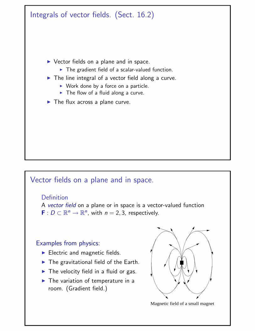
DefinitionA vector field on a plane or in space is a vector-valued functionF : D ⊂ Rn → Rn, with n = 2, 3, respectively.
Examples from physics:
I Electric and magnetic fields.
I The gravitational field of the Earth.
I The velocity field in a fluid or gas.
I The variation of temperature in aroom. (Gradient field.)
Magnetic field of a small magnet.
Integrals of vector fields. (Sect. 16.2)
I Vector fields on a plane and in space.I The gradient field of a scalar-valued function.
I The line integral of a vector field along a curve.I Work done by a force on a particle.I The flow of a fluid along a curve.
I The flux across a plane curve.
The gradient field of a scalar-valued function.
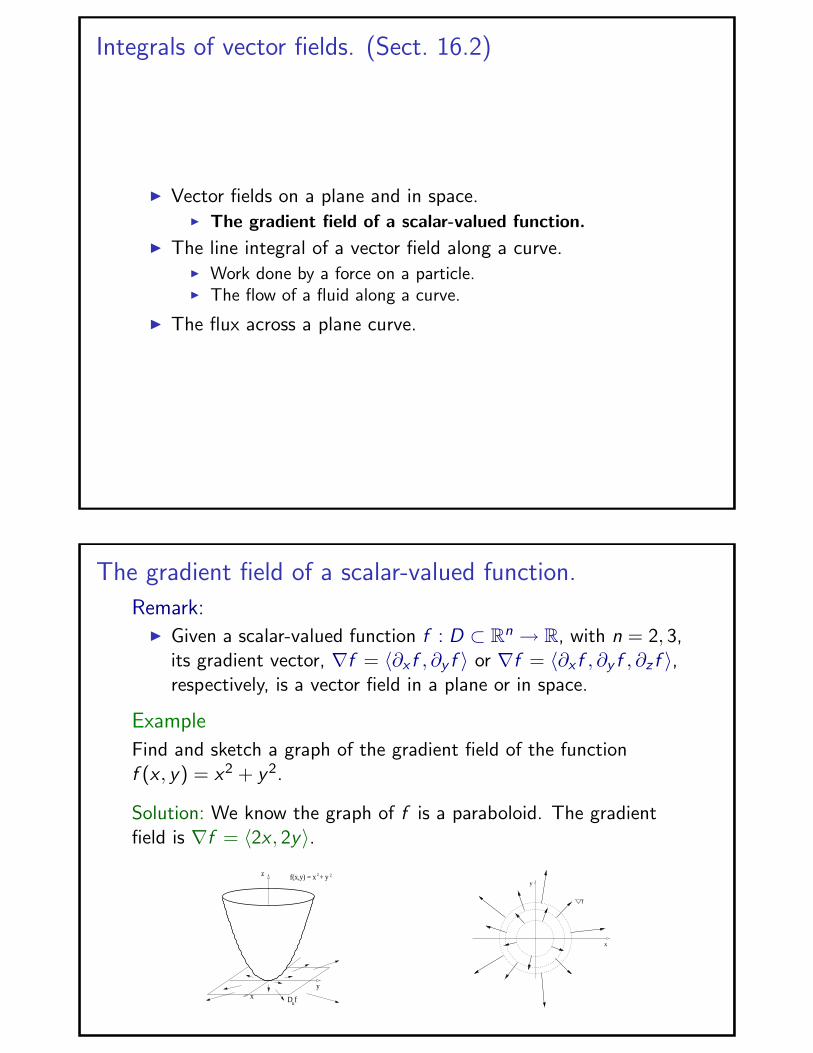
Remark:I Given a scalar-valued function f : D ⊂ Rn → R, with n = 2, 3,
its gradient vector, ∇f = 〈∂x f , ∂y f 〉 or ∇f = 〈∂x f , ∂y f , ∂z f 〉,respectively, is a vector field in a plane or in space.
Example
Find and sketch a graph of the gradient field of the functionf (x , y) = x2 + y2.
Solution: We know the graph of f is a paraboloid. The gradientfield is ∇f = 〈2x , 2y〉.
z f(x,y) = x + y
xy
2 2
D fu
x
y
f
Integrals of vector fields. (Sect. 16.2)
I Vector fields on a plane and in space.I The gradient field of a scalar-valued function.
I The line integral of a vector field along a curve.I Work done by a force on a particle.I The flow of a fluid along a curve.
I The flux across a plane curve.
The line integral of a vector field along a curve.
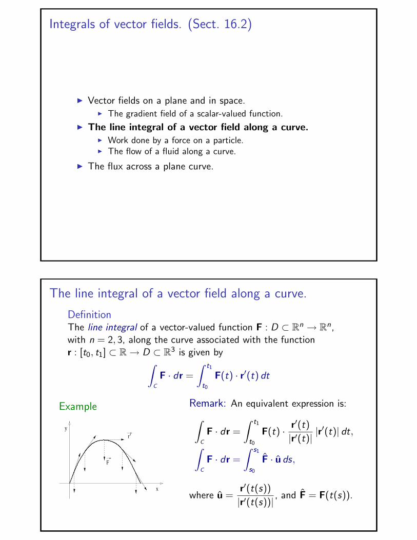
DefinitionThe line integral of a vector-valued function F : D ⊂ Rn → Rn,with n = 2, 3, along the curve associated with the functionr : [t0, t1] ⊂ R → D ⊂ R3 is given by∫
C
F · dr =
∫ t1
t0
F(t) · r′(t) dt
Example
F
y
x
r’
Remark: An equivalent expression is:∫C
F · dr =
∫ t1
t0
F(t) · r′(t)
|r′(t)||r′(t)| dt,∫
C
F · dr =
∫ s1
s0
F · u ds,
where u =r′(t(s))
|r′(t(s))|, and F = F(t(s)).
Integrals of vector fields. (Sect. 16.2)
I Vector fields on a plane and in space.I The gradient field of a scalar-valued function.
I The line integral of a vector field along a curve.I Work done by a force on a particle.I The flow of a fluid along a curve.
I The flux across a plane curve.
Work done by a force on a particle.
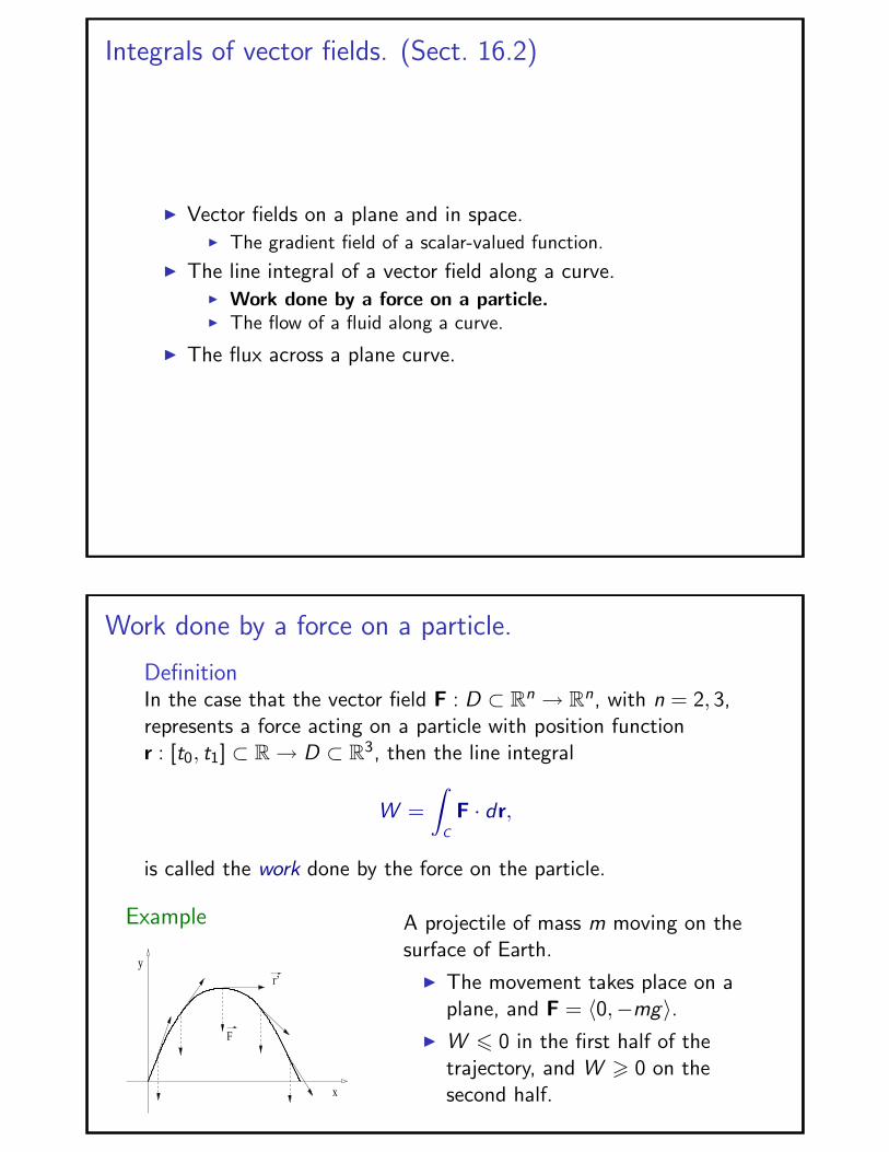
DefinitionIn the case that the vector field F : D ⊂ Rn → Rn, with n = 2, 3,represents a force acting on a particle with position functionr : [t0, t1] ⊂ R → D ⊂ R3, then the line integral
W =
∫C
F · dr,
is called the work done by the force on the particle.
Example
F
y
x
r’
A projectile of mass m moving on thesurface of Earth.
I The movement takes place on aplane, and F = 〈0,−mg〉.
I W 6 0 in the first half of thetrajectory, and W > 0 on thesecond half.
Work done by a force on a particle.
Example
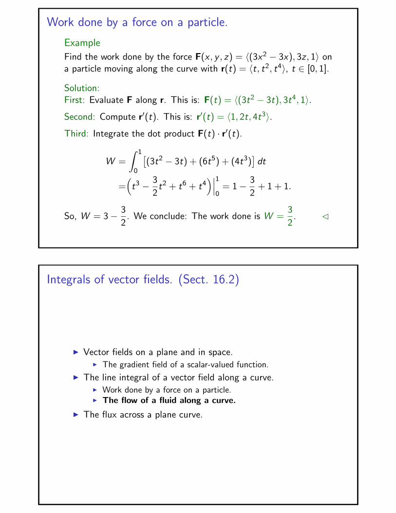
Find the work done by the force F(x , y , z) = 〈(3x2 − 3x), 3z , 1〉 ona particle moving along the curve with r(t) = 〈t, t2, t4〉, t ∈ [0, 1].
Solution:First: Evaluate F along r. This is: F(t) = 〈(3t2 − 3t), 3t4, 1〉.
Second: Compute r′(t). This is: r′(t) = 〈1, 2t, 4t3〉.
Third: Integrate the dot product F(t) · r′(t).
W =
∫ 1
0
[(3t2 − 3t) + (6t5) + (4t3)
]dt
=(t3 − 3
2t2 + t6 + t4
)∣∣∣10
= 1− 3
2+ 1 + 1.
So, W = 3− 3
2. We conclude: The work done is W =
3
2. C
Integrals of vector fields. (Sect. 16.2)
I Vector fields on a plane and in space.I The gradient field of a scalar-valued function.
I The line integral of a vector field along a curve.I Work done by a force on a particle.I The flow of a fluid along a curve.
I The flux across a plane curve.
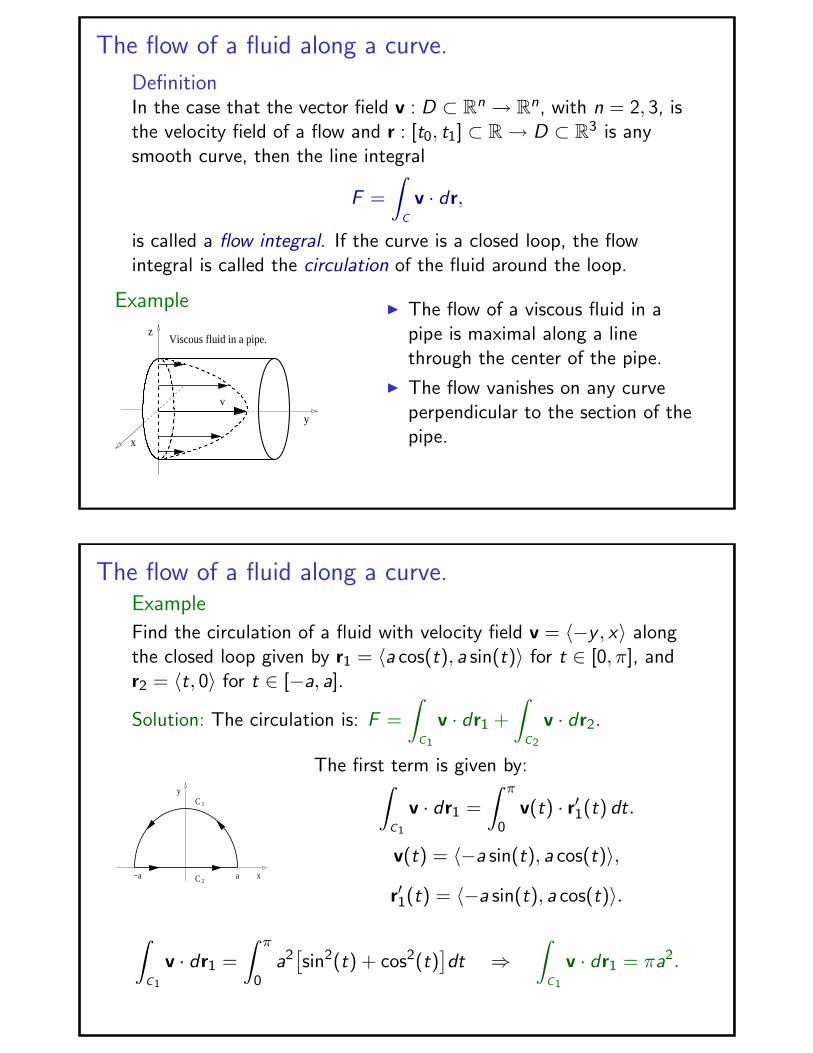
The flow of a fluid along a curve.
DefinitionIn the case that the vector field v : D ⊂ Rn → Rn, with n = 2, 3, isthe velocity field of a flow and r : [t0, t1] ⊂ R → D ⊂ R3 is anysmooth curve, then the line integral
F =
∫C
v · dr,
is called a flow integral. If the curve is a closed loop, the flowintegral is called the circulation of the fluid around the loop.
Example
Viscous fluid in a pipe.
x
z
v
y
I The flow of a viscous fluid in apipe is maximal along a linethrough the center of the pipe.
I The flow vanishes on any curveperpendicular to the section of thepipe.
The flow of a fluid along a curve.Example
Find the circulation of a fluid with velocity field v = 〈−y , x〉 alongthe closed loop given by r1 = 〈a cos(t), a sin(t)〉 for t ∈ [0, π], andr2 = 〈t, 0〉 for t ∈ [−a, a].
Solution: The circulation is: F =
∫C1
v · dr1 +
∫C2
v · dr2.
1
y
x−a aC2
C
The first term is given by:∫C1
v · dr1 =
∫ π
0v(t) · r′1(t) dt.
v(t) = 〈−a sin(t), a cos(t)〉,
r′1(t) = 〈−a sin(t), a cos(t)〉.
∫C1
v · dr1 =
∫ π
0a2
[sin2(t) + cos2(t)
]dt ⇒
∫C1
v · dr1 = πa2.
The flow of a fluid along a curve.
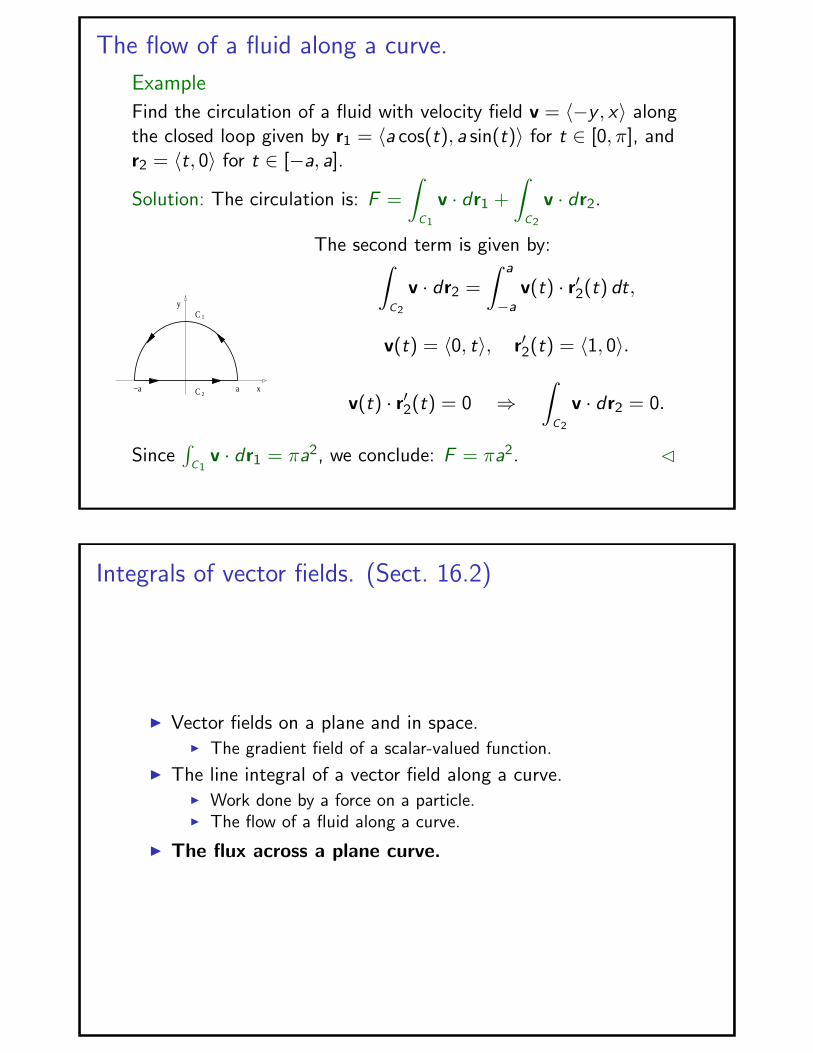
Example
Find the circulation of a fluid with velocity field v = 〈−y , x〉 alongthe closed loop given by r1 = 〈a cos(t), a sin(t)〉 for t ∈ [0, π], andr2 = 〈t, 0〉 for t ∈ [−a, a].
Solution: The circulation is: F =
∫C1
v · dr1 +
∫C2
v · dr2.
1
y
x−a aC2
C
The second term is given by:∫C2
v · dr2 =
∫ a
−av(t) · r′2(t) dt,
v(t) = 〈0, t〉, r′2(t) = 〈1, 0〉.
v(t) · r′2(t) = 0 ⇒∫
C2
v · dr2 = 0.
Since∫
C1v · dr1 = πa2, we conclude: F = πa2. C
Integrals of vector fields. (Sect. 16.2)
I Vector fields on a plane and in space.I The gradient field of a scalar-valued function.
I The line integral of a vector field along a curve.I Work done by a force on a particle.I The flow of a fluid along a curve.
I The flux across a plane curve.
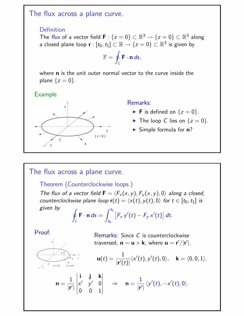
The flux across a plane curve.
DefinitionThe flux of a vector field F : {z = 0} ⊂ R3 → {z = 0} ⊂ R3 alonga closed plane loop r : [t0, t1] ⊂ R → {z = 0} ⊂ R3 is given by
F =
∮C
F · n ds,
where n is the unit outer normal vector to the curve inside theplane {z = 0}.
Example
Cn
{ z = 0 }
y
x
zRemarks:
I F is defined on {z = 0}.I The loop C lies on {z = 0}.I Simple formula for n?
The flux across a plane curve.
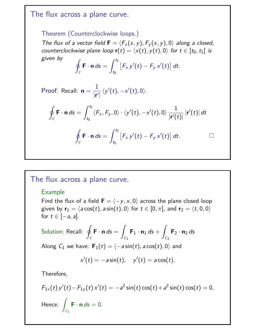
Theorem (Counterclockwise loops.)
The flux of a vector field F = 〈Fx(x , y),Fy (x , y), 0〉 along a closed,counterclockwise plane loop r(t) = 〈x(t), y(t), 0〉 for t ∈ [t0, t1] isgiven by ∮
C
F · n ds =
∫ t1
t0
[Fx y ′(t)− Fy x ′(t)
]dt.
Proof:
n = u x k
y
x
z
C{ z = 0 }
k
u
Remarks: Since C is counterclockwisetraversed, n = u× k, where u = r′/|r′|.
u(t) =1
|r′(t)|〈x ′(t), y ′(t), 0〉, k = 〈0, 0, 1〉.
n =1
|r′|
∣∣∣∣∣∣i j kx ′ y ′ 00 0 1
∣∣∣∣∣∣ ⇒ n =1
|r′|〈y ′(t),−x ′(t), 0〉.
The flux across a plane curve.
Theorem (Counterclockwise loops.)
The flux of a vector field F = 〈Fx(x , y),Fy (x , y), 0〉 along a closed,counterclockwise plane loop r(t) = 〈x(t), y(t), 0〉 for t ∈ [t0, t1] isgiven by ∮
C
F · n ds =
∫ t1
t0
[Fx y ′(t)− Fy x ′(t)
]dt.
Proof: Recall: n =1
|r′|〈y ′(t),−x ′(t), 0〉.
∮C
F · n ds =
∫ t1
t0
〈Fx ,Fy , 0〉 · 〈y ′(t),−x ′(t), 0〉 1
|r′(t)||r′(t)| dt
∮C
F · n ds =
∫ t1
t0
[Fx y ′(t)− Fy x ′(t)
]dt.
The flux across a plane curve.
Example
Find the flux of a field F = 〈−y , x , 0〉 across the plane closed loopgiven by r1 = 〈a cos(t), a sin(t), 0〉 for t ∈ [0, π], and r2 = 〈t, 0, 0〉for t ∈ [−a, a].
Solution: Recall:
∮C
F · n ds =
∫C1
F1 · n1 ds +
∫C2
F2 · n2 ds
Along C1 we have: F1(t) = 〈−a sin(t), a cos(t), 0〉 and
x ′(t) = −a sin(t), y ′(t) = a cos(t).
Therefore,
F1x(t) y ′(t)−F1y (t) x ′(t) = −a2 sin(t) cos(t)+a2 sin(t) cos(t) = 0.
Hence:
∫C1
F · n ds = 0.
The flux across a plane curve.
Example
Find the flux of a field F = 〈−y , x , 0〉 across the plane closed loopgiven by r1 = 〈a cos(t), a sin(t), 0〉 for t ∈ [0, π], and r2 = 〈t, 0, 0〉for t ∈ [−a, a].
Solution: Recall:
∮C
F · n ds =
∫C1
F1 · n1 ds +
∫C2
F2 · n2 ds
Along C2 we have: F2(t) = 〈0, t, 0〉 and x ′(t) = 1, y ′(t) = 0. So,
F2x(t) y ′(t)− F2y (t) x ′(t) = 0− t ⇒∫
C2
F · n ds =
∫ a
−a−t dt,
∫C2
F · n ds = −( t2
2
∣∣∣a−a
)⇒
∫C2
F · n ds = 0.
We conclude:
∮C
F · n ds = 0. C