
Review: Basics of Asymptotic Theory -...
43
Review: Basics of Asymptotic Theory • Classic reference is C.R. Rao (1973): “Linear Statistical Inference and its Applications” • Some of this material has been covered before (241A/B), but it is very important, so we review it here • Agenda: • 1. Convergence of deterministic sequences • 2. Convergence of sequences of random variables • 3. Definitions and “tools” of asymptotic theory Olivier Deschenes, UCSB, Econ 241C, Spring 2016
Transcript of Review: Basics of Asymptotic Theory -...

Review: Basics of Asymptotic Theory
• Classic reference is C.R. Rao (1973): “Linear Statistical Inference and its Applications”
• Some of this material has been covered before (241A/B), but it is very important, so we review it here
• Agenda: • 1. Convergence of deterministic sequences
• 2. Convergence of sequences of random variables
• 3. Definitions and “tools” of asymptotic theory
Olivier Deschenes, UCSB, Econ 241C, Spring 2016

Our approach to asymptotic theory:
• Class presentation will be a limited sketch of these results
• More complete presentations / proofs appear in various textbooks. See Hayashi chapter 2, Wooldridge chapter 3
• We will develop other results as we proceed
Olivier Deschenes, UCSB, Econ 241C, Spring 2016

Motivation: • An important component of econometrics involves nonlinear
models or nonlinear estimation techniques
• The number of exact statistical results that can be obtained in these cases is very low
• Instead, we rely on approximate results that are based on what we know about the behavior of certain statistics in large samples (i.e. as n →∞)
• ⇒ View estimators as sequences of random variables and study their behavior as n →∞ – Allow us to use law of large numbers and central limit theorem
Olivier Deschenes, UCSB, Econ 241C, Spring 2016

Definition of estimator: • An estimator is a rule that assigns a number or a function to
every data set
• Example:
• ‘Rule’ says sum all data on X and divide by n
• Similar view of all estimators in this class (i.e. OLS, etc)
Olivier Deschenes, UCSB, Econ 241C, Spring 2016
∑=
=n
iin X
nX
1
1
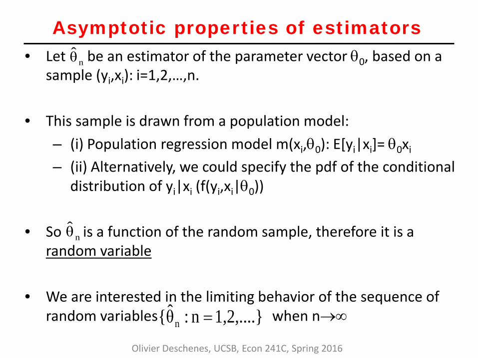
Asymptotic properties of estimators • Let be an estimator of the parameter vector θ0, based on a
sample (yi,xi): i=1,2,…,n.
• This sample is drawn from a population model: – (i) Population regression model m(xi,θ0): E[yi|xi]= θ0xi – (ii) Alternatively, we could specify the pdf of the conditional
distribution of yi|xi (f(yi,xi|θ0)) • So is a function of the random sample, therefore it is a
random variable
• We are interested in the limiting behavior of the sequence of random variables when n→∞ 1,2,....}n:θ̂{ n =
Olivier Deschenes, UCSB, Econ 241C, Spring 2016
θ̂ n
θ̂ n
Consistent estimator • We say that is consistent for θ0 if plim =θ0 for all possible
values of θ0
• Set of possible values for θ0 is called the parameter space (Θ)
• Sometimes parameter space is defined by economic theory. Most of the time we just assume it is a large set (more precise definition to come)
Olivier Deschenes, UCSB, Econ 241C, Spring 2016
θ̂ n θ̂ n
Asymptotically normal estimator • We say that a consistent estimator is asymptotically normal
if:
• Where V is a positive definite matrix • V is the asymptotic variance of
• The asymptotic variance of is V/n
Olivier Deschenes, UCSB, Econ 241C, Spring 2016
θ̂ n
( ) V)N(0, θ-θ̂nd
0n →
( ) θ-θ̂n 0n
θ̂ n

Limits of deterministic sequences: • The sequence {bn : n = 1, 2, 3, …. } of real numbers converge to
the real number b (or has limit b), if for any positive number ε (no matter how small), it is possible to find a positive integer N(ε) such that for all n ≥ N(ε), |bn – b| < ε.
• We write bn→b or
• Examples: {an} = (n-1)/n has limit =1 {bn} = (-1)n+1
• Sequence bn has no limit
bbnn=
∞→lim
Olivier Deschenes, UCSB, Econ 241C, Spring 2016
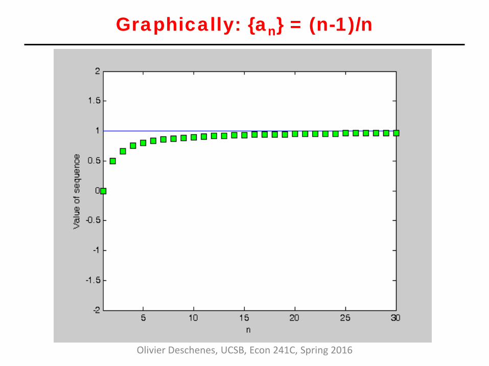
Graphically: {an} = (n-1)/n
Olivier Deschenes, UCSB, Econ 241C, Spring 2016

Graphically: {bn} =(-1)n+1
Olivier Deschenes, UCSB, Econ 241C, Spring 2016

Limits of sequence of deterministic functions
• Different concept of convergence for sequences of functions. Ex: cn(θ) = θn, θ=[0,1) vs θ=[0,1], n=1,2,3,…
• Concepts of “pointwise” and “uniform” convergence
• Uniform convergence preserves continuity of continuous functions in the limits, and that will be important for us in some cases
• Uniform convergence has stronger requirements
• We return to this later
Olivier Deschenes, UCSB, Econ 241C, Spring 2016
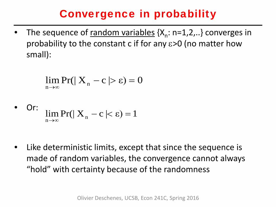
Convergence in probability • The sequence of random variables {Xn: n=1,2,..} converges in
probability to the constant c if for any ε>0 (no matter how small):
• Or:
• Like deterministic limits, except that since the sequence is
made of random variables, the convergence cannot always “hold” with certainty because of the randomness
Olivier Deschenes, UCSB, Econ 241C, Spring 2016
0ε)|cXPr(|lim nn=>−
∞→
1ε)|cXPr(|lim nn=<−
∞→

Interpretation: • In the deterministic case, convergences means that any
deviation between bn and its limit b is eliminated as n increases without bound
• In the stochastic case, convergence in probability means that any deviation between Xn and the limit c is eliminated with probability approaching 1 as n increases without bound
• Key application is Law of Large Numbers
Olivier Deschenes, UCSB, Econ 241C, Spring 2016

• This is also written as:
– Generalizes to sequences of random vectors by requiring convergence in probability of each element of the vector
Olivier Deschenes, UCSB, Econ 241C, Spring 2016
cXplim nn
=∞→
cXp
n →

Example: • Consider the random variable Xi = 1(ith toss of a fair coin is
“tails”) • Pr(Xi = 1) = 0.5 • Consider the sequence of random variables {Xi: i=1,2,….} and
the associated sequence of random variables:
• We already know that plim Yn = 0.5 • Can use Chebyshev’s inequality to prove it formally
∑=
=n
iin X
nY
1
1
Olivier Deschenes, UCSB, Econ 241C, Spring 2016
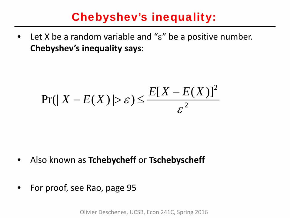
Chebyshev’s inequality: • Let X be a random variable and “ε” be a positive number.
Chebyshev’s inequality says:
• Also known as Tchebycheff or Tschebyscheff
• For proof, see Rao, page 95
2
2)]([)|)(Pr(|ε
ε XEXEXEX −≤>−
Olivier Deschenes, UCSB, Econ 241C, Spring 2016

• Since Xn∼Bernoulli(0.5), we know that E[Xn]=0.5 and Var[Xn]=0.25
• We also know that E[Yn]=0.5 and Var(Yn)=(1/n)*0.25 • Thus:
• So: plim Yn = 0.5 Olivier Deschenes, UCSB, Econ 241C, Spring 2016
22n
n nε0.25
ε)Var(Yε)|0.5YPr(| =≤>−
2nnn nε0.25limε)|0.5YPr(|lim
∞→∞→≤>−
0ε)|0.5YPr(|lim nn=>−
∞→

Graphical illustration of example Xi∼Bernoulli(0.4), Yn=(1/n)ΣXi
Olivier Deschenes, UCSB, Econ 241C, Spring 2016
n=1,..,100
Graphical illustration of example Xi∼Bernoulli(0.4), Yn=(1/n)ΣXi
Olivier Deschenes, UCSB, Econ 241C, Spring 2016
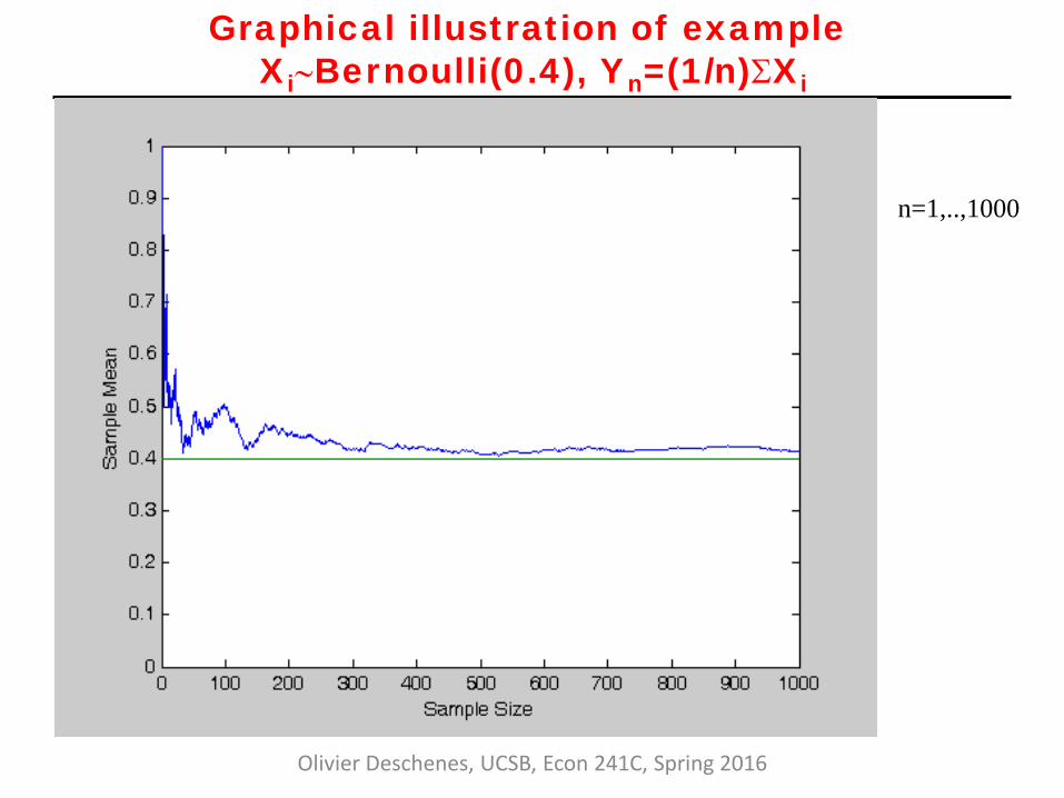
n=1,..,1000

Graphical illustration of example Xi∼Bernoulli(0.4), Yn=(1/n)ΣXi
Olivier Deschenes, UCSB, Econ 241C, Spring 2016
n=1,..,10000
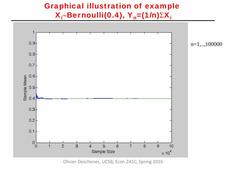
Graphical illustration of example Xi∼Bernoulli(0.4), Yn=(1/n)ΣXi
Olivier Deschenes, UCSB, Econ 241C, Spring 2016
n=1,..,100000
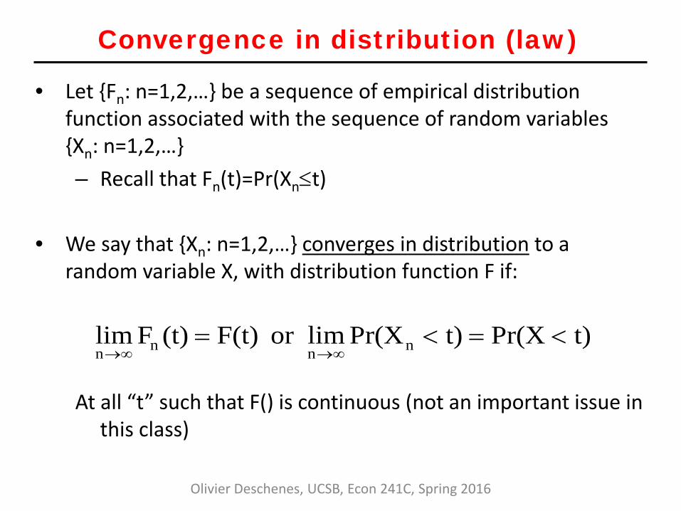
Convergence in distribution (law)
• Let {Fn: n=1,2,…} be a sequence of empirical distribution function associated with the sequence of random variables {Xn: n=1,2,…} – Recall that Fn(t)=Pr(Xn≤t)
• We say that {Xn: n=1,2,…} converges in distribution to a
random variable X, with distribution function F if: At all “t” such that F() is continuous (not an important issue in
this class)
Olivier Deschenes, UCSB, Econ 241C, Spring 2016
t)Pr(Xt)Pr(Xlimor F(t)(t)Flim nnnn<=<=
∞→∞→

• We write
• F is called the asymptotic or limiting distribution of Xn
• The idea of convergence in distribution is that the distribution function of Xn gets closer and closer to distribution function of the random variable X (for which we know the functional form of generally) when n gets large
• Thus, we can use the distribution function of X as an approximation for the distribution function of Xn
• Key application is Central Limit Theorem Olivier Deschenes, UCSB, Econ 241C, Spring 2016
XXor FXd
n
d
n →→
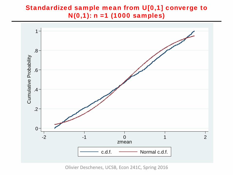
Standardized sample mean from U[0,1] converge to N(0,1): n =1 (1000 samples)
Olivier Deschenes, UCSB, Econ 241C, Spring 2016
0
.2
.4
.6
.8
1C
umul
ativ
e P
roba
bilit
y
-2 -1 0 1 2zmean
c.d.f. Normal c.d.f.

Standardized sample mean from U[0,1] converge to N(0,1): n =3 (1000 samples)
Olivier Deschenes, UCSB, Econ 241C, Spring 2016
0
.2
.4
.6
.8
1C
umul
ativ
e P
roba
bilit
y
-4 -2 0 2 4zmean
c.d.f. Normal c.d.f.

Standardized sample mean from U[0,1] converge to N(0,1): n =30 (1000 samples)
Olivier Deschenes, UCSB, Econ 241C, Spring 2016
0
.2
.4
.6
.8
1C
umul
ativ
e P
roba
bilit
y
-4 -2 0 2 4zmean
c.d.f. Normal c.d.f.

Standardized sample mean from U[0,1] converge to N(0,1): n =300 (1000 samples)
Olivier Deschenes, UCSB, Econ 241C, Spring 2016
0
.2
.4
.6
.8
1C
umul
ativ
e P
roba
bilit
y
-4 -2 0 2 4zmean
c.d.f. Normal c.d.f.

Standardized sample mean from U[0,1] converge to N(0,1): n =3000 (1000 samples)
Olivier Deschenes, UCSB, Econ 241C, Spring 2016
0
.2
.4
.6
.8
1C
umul
ativ
e P
roba
bilit
y
-4 -2 0 2 4zmean
c.d.f. Normal c.d.f.

Relationship among modes of convergence
• Key result:
• Proof: Use Chebyshev’s inequality
Olivier Deschenes, UCSB, Econ 241C, Spring 2016
cX cXd
n
p
n →⇒→
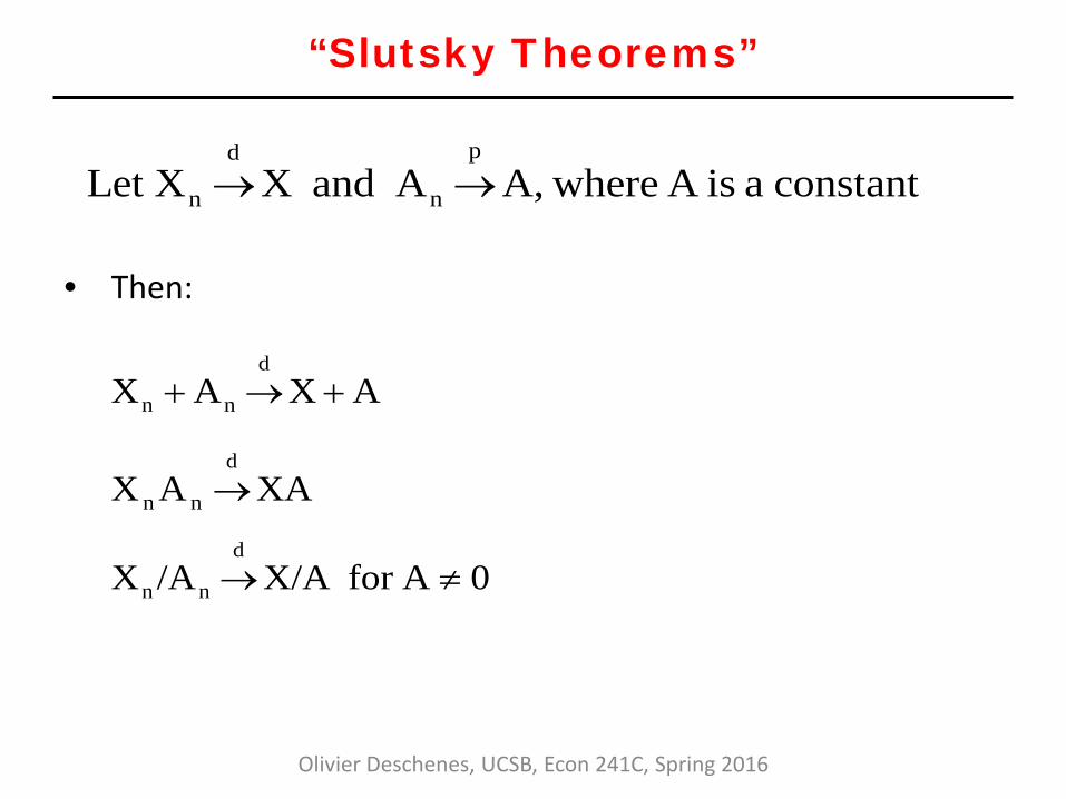
“Slutsky Theorems”
• Then:
Olivier Deschenes, UCSB, Econ 241C, Spring 2016
constant a isA whereA,A and XXLet p
n
d
n →→
AXAXd
nn +→+
XAAXd
nn →
0Afor X/A /AXd
nn ≠→

‘Product Limit Normal Rule’
• Let and
• Then:
• Just an application of Slutsky to the normal distribution
• We will use this a lot
Olivier Deschenes, UCSB, Econ 241C, Spring 2016
AAp
n → ),( Σ→ µNXd
n
)',( AAANXAd
nn Σ→ µ

Continuous mapping theorem • Let g(.) be a continuous function. The CMT states that:
• The CMT is a very useful tool for asymptotic analysis since it applies to non-linear functions (as long as they are continuous) – Example: the expectation operator E(.) does not have this
property
Olivier Deschenes, UCSB, Econ 241C, Spring 2016
=→⇒→
∞→∞→n
nn
n
p
n
p
n Xplimg)g(Xplim i.e., g(c))g(X cX
g(X))g(X XXd
n
d
n →⇒→
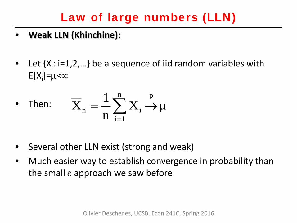
Law of large numbers (LLN) • Weak LLN (Khinchine): • Let {Xi: i=1,2,…} be a sequence of iid random variables with
E[Xi]=µ<∞
• Then:
• Several other LLN exist (strong and weak) • Much easier way to establish convergence in probability than
the small ε approach we saw before
Olivier Deschenes, UCSB, Econ 241C, Spring 2016
μXn1X
pn
1iin →= ∑
=
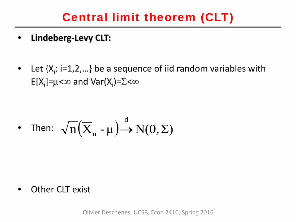
Central limit theorem (CLT) • Lindeberg-Levy CLT: • Let {Xi: i=1,2,…} be a sequence of iid random variables with
E[Xi]=µ<∞ and Var(Xi)=Σ<∞
• Then:
• Other CLT exist
Olivier Deschenes, UCSB, Econ 241C, Spring 2016
( ) Σ)N(0, μ-Xnd
n →

Example: CLT in action • Consider the following experiment:
• Draw a sample of size “n” from the Uniform [0,1] distribution
and calculate the sample mean
• Rescale by subtracting population mean (0.5), multiplying by √n and dividing by standard deviation (1/12)
• CLT says that as “n” grows large, distribution of rescaled sample mean should get closer and closer to a Normal distribution (here N(0,1))
Olivier Deschenes, UCSB, Econ 241C, Spring 2016

n=1 (1,000 samples)
Olivier Deschenes, UCSB, Econ 241C, Spring 2016
0.0
2.0
4.0
6.0
8.1
Frac
tion
-4 -2 0 2 4zmean
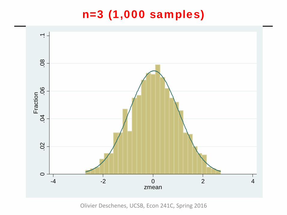
n=3 (1,000 samples)
Olivier Deschenes, UCSB, Econ 241C, Spring 2016
0.0
2.0
4.0
6.0
8.1
Frac
tion
-4 -2 0 2 4zmean

n=30 (1,000 samples)
Olivier Deschenes, UCSB, Econ 241C, Spring 2016
0.0
2.0
4.0
6.0
8.1
Frac
tion
-4 -2 0 2 4zmean
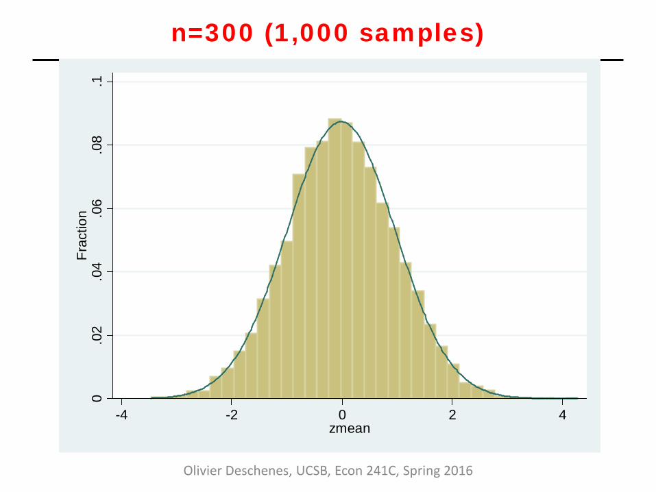
n=300 (1,000 samples)
Olivier Deschenes, UCSB, Econ 241C, Spring 2016
0.0
2.0
4.0
6.0
8.1
Frac
tion
-4 -2 0 2 4zmean
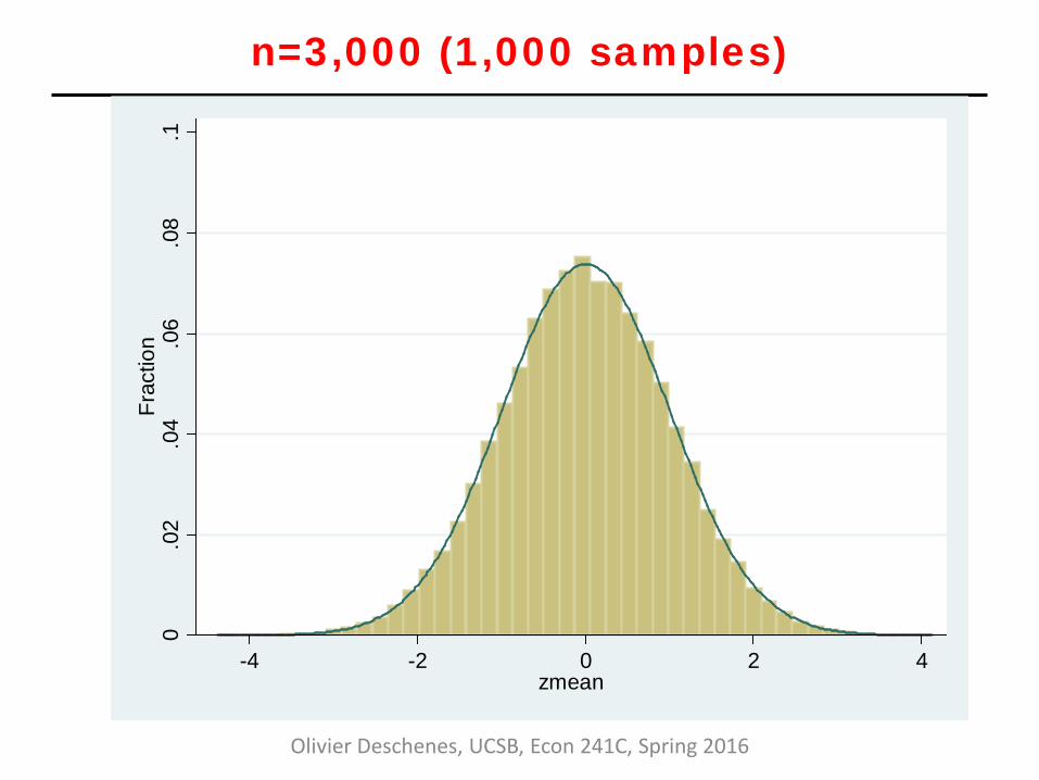
n=3,000 (1,000 samples)
Olivier Deschenes, UCSB, Econ 241C, Spring 2016
0.0
2.0
4.0
6.0
8.1
Frac
tion
-4 -2 0 2 4zmean
Other tools / concepts • Delta-method
• Mean-value expansion (to come)
• Asymptotically-linear estimators (to come)
• Asymptotic equivalence (to come)
Olivier Deschenes, UCSB, Econ 241C, Spring 2016
Olivier Deschenes, UCSB, Econ 241C, Spring 2016
“Delta Method”
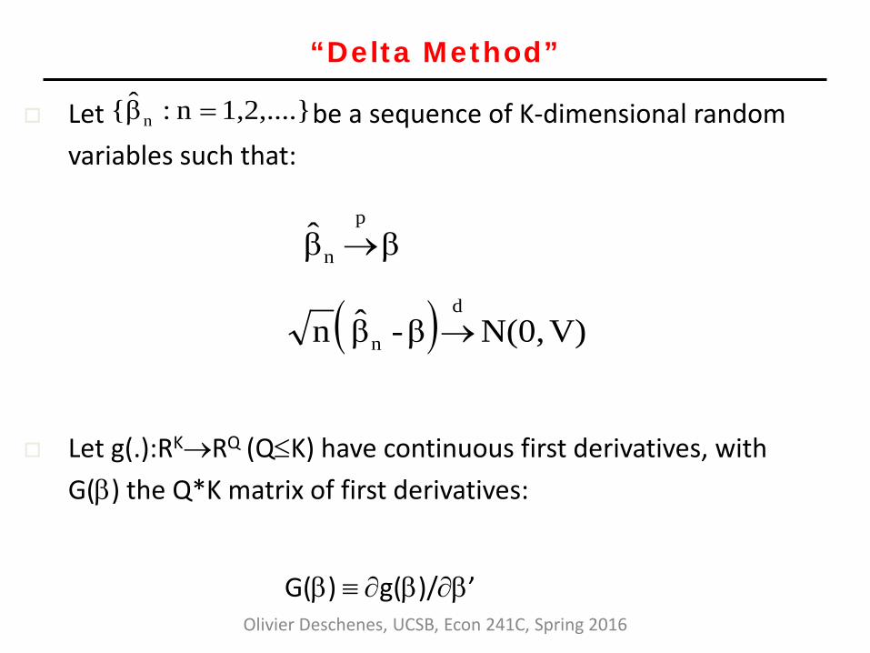
Let be a sequence of K-dimensional random variables such that:
Let g(.):RK→RQ (Q≤K) have continuous first derivatives, with G(β) the Q*K matrix of first derivatives:
G(β) ≡ ∂g(β)/∂β’
1,2,....}n:β̂{ n =
ββ̂ p
n →
( ) V)N(0, β-β̂ nd
n →
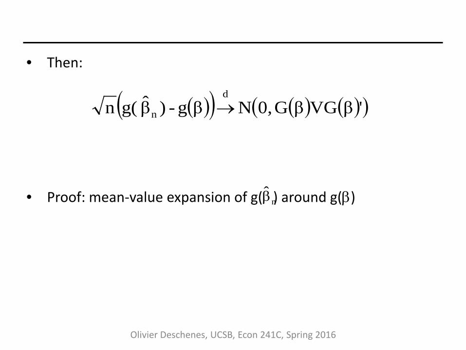
• Then:
• Proof: mean-value expansion of g( ) around g(β)
Olivier Deschenes, UCSB, Econ 241C, Spring 2016
( )( ) ( ) ( )( )'βVGβG0,N βg-)β̂ g(nd
n →
β̂ n


