Review and Rating Discharge

Measurements

Review and Rating Discharge

MeasurementsDavid S. Mueller

Office of Surface Water

March 2010

OverviewOverview Considerations in Rating a Measurement Six Review Steps

Gather information for rating as you review Three Examples

Rating ProcessRating Process Quantitative assessment of measurement

uncertainty Currently being worked on

Current practice is subjective Where we can quantify we will Where we can’t we will make qualitative estimates

Rating ConsiderationsRating Considerations Variability of transect discharges Pattern in transect discharges Accuracy of top and bottom extrapolation Accuracy of edge extrapolation Quantity and distribution of missing data Quality of boat navigation reference

Bias or noise in bottom track Noise in GPS data

Spread in Transect Discharges

Spread in Transect Discharges

A coefficient of variation (COV) is computed by the software (Std./|Avg.|)

The COV represents the sampled random error in the discharge measurement.

Dividing the COV by the sqrt of the number of passes and multiplying by the correct value will provide the 95% uncertainty associated with random errors as measured For 4 passes: 1.6*COV For 8 passes: 0.8*COV This does not include any bias errors This is probably and optimistic estimate

Example of Random ErrorExample of Random Error

95% Uncertainy (Random Error) = 0.05*0.8 = 4%

Patterns in TransectsPatterns in Transects Random errors should not display a pattern A pattern in flow may indicate the need to

adjust measurement procedures Rapidly rising or falling – average fewer transects Periodic – use more transects to capture

variability

Top ExtrapolationTop Extrapolation Average appropriate number of ensembles Evaluate discharge profile Check field notes for wind effects Try different extrapolation methods and

compare change in total discharge Little change – accurate extrapolation likely Significant change – how good is the data on

which the selection is made Surface effects captured? Field notes consistent with pattern?

What percentage of flow is in the top portion Subjective judgment

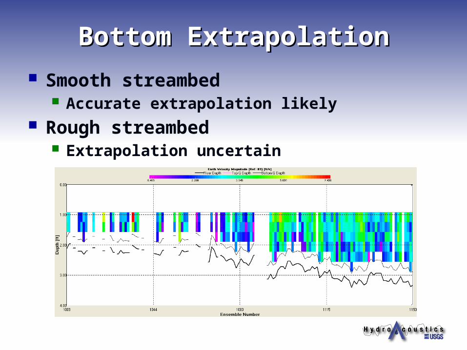
Bottom ExtrapolationBottom Extrapolation Smooth streambed

Accurate extrapolation likely Rough streambed

Extrapolation uncertain

Edge EstimatesEdge Estimates What percentage of flow is in the edges?

May be small enough to disregard accuracy Recommend no more than 5% in each edge

Subjective judgment Large edge estimates Irregular edge shapes

Edge Q = 25% of total

Invalid DataInvalid Data Percent of invalid data Distribution of invalid data How well is that portion of the flow estimated

Summary of Rating Approach

Summary of Rating Approach

Consider the data Consider the hydraulics Consider site conditions Use statistics, if possible Use your judgment Pay attention to potential errors (as a

percentage) as you review the data

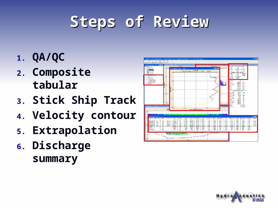
Steps of ReviewSteps of Review

1. QA/QC

2. Composite tabular

3. Stick Ship Track

4. Velocity contour

5. Extrapolation

6. Discharge summary

QA/QCQA/QC ADCP Test Error Free? Compass Calibration

Calibration and evaluation completed

< 1 degree error Important for Loop and GPS

Moving-Bed Test Loop

Requires compass calibration Use LC to evaluate

Stationary Duration and Deployment SMBA required to evaluate

StreamPro

Composite TabularComposite Tabular Number of Ensembles

> 150 ??? Lost Ensembles

Communications error Bad Ensembles

Distribution more important than percentage

Distribution evaluated in velocity contour plot

Reasonable temperature

Stick Ship TrackStick Ship Track Check with appropriate

reference (BT, GGA, VTG) Track and sticks in

correct direction Magnetic variation Heading time series

Sticks representative of flow WT thresholds

Irregular ship track? BT thresholds BT 4-beam solutions

Velocity ContourVelocity Contour Patterns in velocity

distribution Nonuniform Unnatural WT Thresholds

Spikes in bottom profile Turn on Screen Depth

Distribution of invalid and unmeasured areas Qualitative assessment

of uncertainty

Velocity ExtrapolationVelocity Extrapolation Average ensembles (10-20) Evaluate several transects Use Power/Power as default

Find reasons to deviate from Power/Power

Don’t waste time where there is little difference

In doubt try different options an evaluate change in discharge

Helps evaluate potential uncertainty from extrapolation

Person collecting data gets benefit of doubt

Discharge SummaryDischarge Summary Transects within 5% Directional bias

GPS used Magvar correction

Consistency Discharges (top, meas., bottom, left, right) Width, Area Boat speed, Flow Speed, Flow Dir.

Example 1 – Compass Cal.Example 1 – Compass Cal. Compass

Evaluation is Good!

Example 1 – Moving-Bed Test

Example 1 – Moving-Bed Test

Loop looks good LC finds no

problems with loop Lost BT Compass Error No moving-bed

correction required

Example 1 – Composite Tabular

Example 1 – Composite Tabular

> 300 ensembles No lost ensembles 0-1 bad ensembles Temperature

reasonable

Example 1 – Ship Track / Contour

Example 1 – Ship Track / Contour

Ship track consistent No spikes in streambed

in contour plot No hydraulically

unusual patterns Unmeasured areas

reasonable in size

Example 1 - ExtrapolationExample 1 - Extrapolation Top extrapolation a bit

uncertain Try Power/Power

Changed Q = 0.6% Const / No Slip = OK

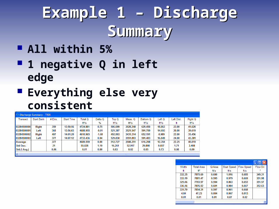
Example 1 – Discharge Summary

Example 1 – Discharge Summary

All within 5% 1 negative Q in left edge Everything else very

consistent

Example 1 - RatingExample 1 - Rating Base uncertainty

1.6*0.01= 1.6% Invalid Data

None Extrapolation

0.5-1% uncertainty in extrapolation Top is only about 10% of total

Edges About 1% of total Q

Final assessment Rate this measurement “GOOD”

Example 2 – QA/QCExample 2 – QA/QC No test errors Compass Cal

High pitch and roll Moving-bed tests

Bottom track problems

Example 2 – Bottom Track Issue

Example 2 – Bottom Track Issue

Time series plots show spikes 3-beam solution High vertical velocity

Example 2 – Composite Tabular

Example 2 – Composite Tabular

Too few ensembles Short duration Bad ensembles

Example 2 – Ship Track / Contour

Example 2 – Ship Track / Contour

Irregular ship track Thresholds didn’t help

No spikes in streambed Invalid data

Not many High percentage because

of so few ensembles Estimates probably

reasonable Large unmeasured areas

% measured < 20%

Example 2 - ExtrapolationExample 2 - Extrapolation Averaged 10 Highly variable Difference between Power/Power and

Constant / No Slip is 3.6% Uncertain about extrapolation accuracy

Example 2 – Discharge Summary

Example 2 – Discharge Summary

Not within 5% 8 passes

Consistent edges Inconsistent width and area

Bottom track problems High Q COV

Example 2 - RatingExample 2 - Rating Base uncertainty

0.14 * 0.8 = 10% Invalid data

Some but not significant Too few ensembles (or too few transects) Bottom track problems Large unmeasured areas

Extrapolation Power/Power to Constant/No Slip = 3.6%

Edges Reasonable

Final Assessment Rate this measurement “POOR”

Example 3 – QA/QCExample 3 – QA/QC No errors in ADCP test Good compass

calibration Two loop tests

Example 3 – Composite Tabular

Example 3 – Composite Tabular

High percentage of bad ensembles

Example 3 – Composite Tabular

Example 3 – Composite Tabular

Very few bad ensembles with reference set to GGA!!

Example 3 – Ship Track / Contour

Example 3 – Ship Track / Contour

Everything looks good with reference set to GGA

Example 3 – Ship Track / Contour

Example 3 – Ship Track / Contour

With bottom track we need to qualitatively assess the effect of the invalid data on uncertainty

Example 3 - ExtrapolationExample 3 - Extrapolation Given the variability among the profile plots

constant / no slip seems reasonable. Changing to power / power made no

difference in the final Q Might justify power / power

Example 3 – Discharge Summary

Example 3 – Discharge Summary

Small directional bias Typical of magvar or compass error with GPS Adjusting magvar 2.5 degrees removed

directional bias and changed Q by 1.3 cfs. Edge discharge are inconsistent but small

relative to total Q

Example 3 – Discharge Summary

Example 3 – Discharge Summary

Bottom track referenced discharge are lower indicating a moving bed was present.

Edge discharges are inconsistent but small Would require correction with LC

Example 3 - RatingExample 3 - Rating GPS (GGA or VTG) should be used as the

reference. Base uncertainty

0.03 * 1.6 = 4.8% Value inflated due to directional bias

No significant invalid data Extrapolation and edges would make little

difference Final assessment

Could rate this measurement “Good” wouldn’t argue much if rated “Fair”

Example 3 - RatingExample 3 - Rating If GPS were not available and BT had to be used the rating would

change. Loops

High percentage of invalid bottom track 5-8% moving-bed bias

Base uncertainty 0.02 * 1.4 = 3.2%

Invalid data Represent a significant percentage of the flow Likely estimated well from neighboring data

Edges Inconsistent Small percentage

Extrapolation Errors very small

Final assessment Loop correction probably within 4% + 3.2% random error I would probably rate this measurement “Fair”

SummarySummary Consider potential uncertainty or errors as you

review the data Keep review to a minimum unless errors are

identified or suspected Consider the percent of effect of an error or

uncertainty will have on the discharge Extrapolation uncertainty can be large in

shallow streams Use the COV in the discharge summary as the

base minimum uncertainty Contact OSW if you have unusual data or you

have questions

Questions???Questions???