Review and Enhancement for Crash Analysis and Prediction ...

MD-10-SP808B4C

Beverley K. Swaim-Staley, Secretary Neil J. Pedersen, Administrator

Martin O’Malley, Governor Anthony G. Brown, Lt. Governor

STATE HIGHWAY ADMINISTRATION

RESEARCH REPORT

Review and Enhancement for Crash Analysis and Prediction: Phase 1-Evaluation of the Crash Studies and Analysis Standard Operating

Procedures in Maryland

Dr. Jie Yu, Dr. H. W. Ho, and Dr. Gang-Len Chang

DEPARTMENT OF CIVIL AND ENVIRONMENTAL ENGINEERING UNIVERSITY OF MARYLAND COLLEGE PARK, MD 20742

April 2010

The contents of this report reflect the views of the author who is responsible for the facts and the accuracy of the data presented herein. The contents do not necessarily reflect the official views or policies of the Maryland State Highway Administration. This report does not constitute a standard, specification, or regulation.

Technical Report Documentation Page

1. Report No. MD-10- SP808B4C

2. Government Accession No. 3. Recipient's Catalog No.

4. Title and Subtitle Review and Enhancement for Crash Analysis and Prediction: Phase 1-Evaluation of the Crash Studies and Analysis Standard Operating Procedures in Maryland

5. Report Date April 16th, 2010

6. Performing Organization Code

7. Author/s Jie Yu, H. W. Ho, and G. L. Chang

8. Performing Organization Report No.

9. Performing Organization Name and Address University of Maryland, Department of Civil and Environmental Engineering, Maryland, College Park, MD 20742

10. Work Unit No. (TRAIS) 11. Contract or Grant No.

SP808B4C 12. Sponsoring Organization Name and Address Maryland State Highway Administration Office of Policy & Research 707 North Calvert Street Baltimore, MD 21202

13. Type of Report and Period CoveredFinal Report

14. Sponsoring Agency Code (7120) STMD - MDOT/SHA

15. Supplementary Notes 16. Abstract

This study offers a comprehensive review of the safety improvement programs adopted by Maryland, FHWA (SafetyAnalyst), and other state agencies, focusing mainly on the following imperative issues: (1) screening and ranking high-crash locations, (2) prioritizing cost-effective projects for safety improvement; and (3) conducting before/after studies for project implementation plans. Based on the resultsof this review, we recommend that the following enhancements be incorporated into the existing safety improvement program in Maryland: (1) develop a multi-criteria method to enhance the current procedures used by the Maryland SHA to select and rank high-crash locations; (2) using SPFs and the observed crash frequency to reliably estimate the site-specific crash frequency: (3) developing and calibrating SPFs for Maryland:; (4) using negative binomial distribution to represent the variation of crash frequency; (5) developing and calibrating the crash reduction functions with local data; (6) including secondary costs/benefits in the evaluation; (7) using SPFs of the after period in estimating the do-nothing crash frequency; and (8) Employing nonlinear models for estimating future traffic volume. 17. Key Words Safety, crash analysis, SafetyAnalyst SPF

18. Distribution Statement: No restrictions This document is available from the Research Division upon request.

19. Security Classification (of this report) None

20. Security Classification (of this page) None

21. No. Of Pages 56

22. Price

Form DOT F 1700.7 (8-72) Reproduction of form and completed page is authorized.

Review and Enhancement for Crash Analysis and Prediction: Phase 1-Evaluation of the Crash Studies and Analysis Standard Operating

Procedures in Maryland

(A final report)

To

Office of Policy and Research

Maryland State Highway Administration

707 N. Calvert Street

Baltimore, MD 21202

by

Dr. Gang-Len Chang, Professor

[email protected]

Dr. Jie Yu and Dr. H. W. Ho, Assistant Research Scientists

Department of Civil Engineering

The University of Maryland

College Park, MD 20742

March 2010

mailto:[email protected]

TABLE OF CONTENTS

TABLE OF CONTENTS .................................................................................................. i

CHAPTER 1 INTRODUCTION ..................................................................................... 1

1.1 RESEARCH BACKGROUND ................................................................................ 1

1.2 RESEARCH OBJECTIVES ..................................................................................... 2

1.3 REPORT ORGANIZATION .................................................................................... 2

CHAPTER 2 OVERALL RESEARCH FRAMEWORK ............................................. 4

2.1 INTRODUCTION .................................................................................................... 4

2.2 RESEARCH TASKS AND OVERALL FLOWCHART ......................................... 5

2.3 CONCLUSION ......................................................................................................... 8

CHAPTER 3 SCREENING OF HIGH-CRASH LOCATIONS .................................. 9

3.1 INTRODUCTION .................................................................................................... 9

3.2 MARYLAND PROCEDURES ................................................................................ 9

3.3 SAFETYANALYST PROCEDURES .................................................................... 13

3.4 METHODS USED BY OTHER STATES ............................................................. 17

3.5 RECOMMENDATIONS ........................................................................................ 24

CHAPTER 4 COST/BENEFIT ANALYSIS ................................................................ 26

4.1 INTRODUCTION .................................................................................................. 26

4.2 MARYLAND PROCEDURES FOR COST/BENEFIT ANALYSIS .................... 26

4.3 SAFETYANALYST PROCEDURES .................................................................... 29

4.4 PROCEDURES USED BY THE STATE OF INDIANA ...................................... 32


CHAPTER 5 COUNTERMEASURE EVALUATION ............................................... 37

i

ii

5.1 INTRODUCTION .................................................................................................. 37

5.2 MARYLAND PROCEDURES .............................................................................. 37

5.3 PROCEDURES USED IN SAFETYANALYST ................................................... 40

5.4 PROCEDURES BY OTHER STATES .................................................................. 43


CHAPTER 6 CONCLUSIONS AND RECOMMENDATIONS ................................ 46

6.1 SUMMARY OF RESEARCH FINDINGS ............................................................ 46

6.2 CONCLUSION ....................................................................................................... 47

REFERENCES ................................................................................................................ 49

APPENDIX- I: THE REGRESSION-TO-THE-MEAN PROBLEM ....................... 51

APPENDIX- II: THE EMPIRICAL BAYESIAN (EB) APPROACH ...................... 53

CHAPTER 1 INTRODUCTION

1.1 RESEARCH BACKGROUND

Traffic safety has become one of the most critical issues facing transportation

agencies across the nation. In 2006, about 43,000 people were killed, and another

290,000 were seriously injured in crashes on public roadways in the United States.

According to a study by the American Automobile Association, traffic crashes in urban

areas cost $164 billion in 2005, including the costs of property damage, lost earnings,

medical treatment, emergency services, pain and lost quality of life, and other costs

(GAO, 2008).

In recent years, federal, state and local transportation/highway agencies have

increasingly dedicated themselves to introducing policies and practices for improving

safety and efficiency of transportation systems. The Safe, Accountable, Flexible, and

Efficient Transportation Equity Act: A Legacy for Users (SAFETEA-LU), which was

enacted on August 10, 2005, established the Highway Safety Improvement Program

(HSIP) as a core federal-aid program (FHWA, 2008). The purpose of this program is to

achieve a significant reduction in traffic fatalities and serious injuries on all public roads

through the implementation of infrastructure-related highway safety improvements. In an

effort to provide a safe highway system to users and to take maximum advantage of

available federal safety funding, the Maryland State Highway Administration (MDSHA)

has developed standard operating procedures (SOPs) for HSIP that consists of four

components: 1) development and implementation of a Strategic Highway Safety Plan

(SHSP) that identifies and analyzes highway safety problems and the potential for

reducing fatalities and serious injuries; 2) production of projects or strategies to reduce

identified safety problems; 3) evaluation of the proposed plans on a regular basis to

ensure the accuracy of the data and the priority of improvements; and 4) submission of an

annual report to the Federal Highway Administration (FHWA) (MDSHA, 2007a).

Well-designed SOPs could effectively help identify the locations for

implementing safety measures. However, the lack of an in-depth study of critical issues in

the SOPs could lead to decisions that fail to alleviate, or even exacerbate, existing traffic

1

safety problems. It is, therefore, imperative to evaluate the current SOPs and to identify

potential improvements to better assist traffic professionals in enhancing highway safety.

1.2 RESEARCH OBJECTIVES

The primary objective of this study is to identify the deficiencies of current crash

studies and analysis SOPs in Maryland and to recommend possible improvements. This

study will focus on the following critical issues:

• Can the current procedures for determining candidate locations for safety

improvement truly identify the high-risk locations?

• Does the current method for cost/benefit analyses effectively prioritize different

improvement plans?

• Can the current methodology for before/after studies reliably measure the

effectiveness of different improvement plans?

The research results with respect to the above issues will offer the basis for SHA

to: (1) better understand the strengths and weaknesses of the current SOPs and to

minimize the cost associated with its implementation; and (2) define potential directions

for improving the SOPs.

1.3 REPORT ORGANIZATION

Based on the research objectives, this study has organized all primary results and

key findings into the five subsequent chapters. A brief description of the information

contained in each chapter is presented below.

Chapter 2, after providing an overview of the current crash studies and analysis

SOPs in Maryland, illustrates the overall research framework and outlines critical project

tasks, along with major activities.

Chapter 3 offers a comprehensive comparison of available methods for screening

high-crash locations, based on an in-depth review of the procedures adopted in Maryland

and other states. The chapter also presents recommendations for improving Maryland’s

currently adopted methodology for screening high-crash locations.

Chapter 4 reviews the procedures for cost/benefit analyses adopted by the

Maryland SHA, SafetyAnalyst and other states. This chapter also includes

recommendations for potential improvements.

2

3

Chapter 5 presents a review of state-of-the-art and state-of-the-practice studies

associated with the countermeasure evaluation procedures adopted by the Maryland SHA,

SafetyAnalyst, and other states. This chapter also describes potential improvements to

overcome some deficiencies identified in the current Maryland countermeasure

evaluation for crash studies and analysis.

Overall research findings and future research needs constitute the core of the final

chapter.

CHAPTER 2 OVERALL RESEARCH FRAMEWORK

2.1 INTRODUCTION

In an effort to reduce the number of crashes, traffic fatalities, and serious injuries on

public roads, Congress passed and President Bush signed SAFETEA-LU in August 2005.

The Act nearly doubled the amount of federal funding for the HSIP by authorizing $5.1

billion from 2006 through 2009 (GAO, 2008). To ensure that the HSIP is carried out in an

organized and systematic manner to achieve the most benefits, the FHWA established a

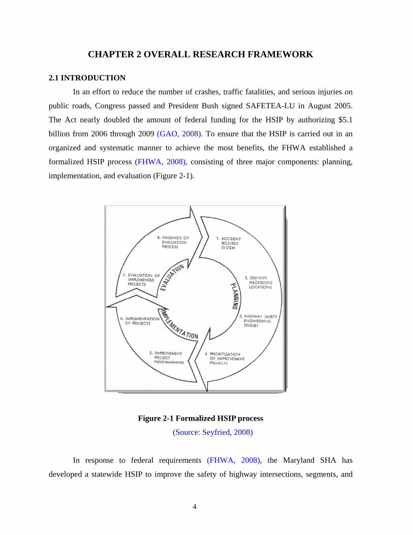
formalized HSIP process (FHWA, 2008), consisting of three major components: planning,

implementation, and evaluation (Figure 2-1).

Figure 2-1 Formalized HSIP process

(Source: Seyfried, 2008)

In response to federal requirements (FHWA, 2008), the Maryland SHA has

developed a statewide HSIP to improve the safety of highway intersections, segments, and

4

ramps that have been identified as Candidate Safety Improvement Locations (CSIL). The

overall SOPs are illustrated in Figure 2-2 (MDSHA, 2007a).

Figure 2-2 Overall SOPs in Maryland’s HSIP

This research will focus on comparing the procedures used by the Maryland SHA in

planning and evaluating safety improvement plans with those adopted by other states and the

federal government.

This chapter is organized as follows: Section 2.2 divides the research work into four

tasks and reports the critical issues associated with each task. Section 2.3 summarizes the

comments on the overall research framework.

2.2 RESEARCH TASKS AND OVERALL FLOWCHART

To complete the research objectives outlined in Chapter 1, the study has focused on

the following tasks:

Task 1: Performing an in-depth review of the current procedures for identifying

high-crash locations and for evaluating effectiveness of safety

improvement plans.

Task 2: Identifying the embedded deficiencies of the current crash studies and

analysis SOPs.

5

Task 3: Recommending improvements to the current crash studies and analysis

SOPs.

Task 4: Producing technical reports and holding workshops to highlight research

findings.

Figure 2-3 shows the overall research flowchart. A brief description of each task is

presented below:

Task 1: Performing an in-depth review of the current procedures for identifying high-

crash locations and for evaluating the effectiveness of safety improvement plans

In performing this task, the research team will extensively review the currently

adopted procedures from the following institutes:

a) Maryland SHA;

b) FHWA; and

c) similar procedures available from other states.

The review will focus on the following critical issues:

a) criteria for screening and sorting high-crash locations;

b) indicators used to quantify the effectiveness of safety improvement plans;

c) assumptions made in the procedures; and

d) types and sources of data required for the evaluation.

Task 2: Identifying the deficiencies of the current crash studies and analysis SOPs.

The criteria adopted in this task for identifying the deficiencies in the procedures used

by the Maryland SHA are summarized below:

a) Effectiveness and efficiency — Used to measure the effectiveness of the

Maryland SOPs in identifying high-crash locations and to evaluate safety

improvement plans.

b) Theoretical and/or statistical support — Used to measure the soundness of the

theoretical basis underlying the currently adopted SOPs.

c) Reasonableness of assumptions made.

d) Practicality — This refers to data needs and required staff skills.

Using these criteria, this task will report on the areas in the current Maryland SOPs

that need some improvement.

6

Task 3: Recommendations for possible improvements in the current crash studies and

analysis SOPs

This task focuses mainly on recommending methods for improving Maryland’s

current crash studies and analysis SOPs. The recommended methods shall overcome some or

all the deficiencies identified in Task 2. The areas of potential improvement include:

a) Procedures for screening and sorting the high-crash locations.

b) Procedures for cost/benefit analyses.

c) Procedures for before/after studies.

The recommendations made in this task will include possible methods for improving

the data, as well as detailed mathematical procedures for implementation.

Task 4: Producing technical reports and conducting workshops to highlight research

findings.

After the annual list of high-crash locations has been generated and evaluated along

with the current crash studies and analysis SOPs, it is important to ensure that potential users

know the embedded deficiencies. Therefore, it is essential to document the findings and

recommendations from this study. The research team will perform the following activities

during this final task:

a) Present research findings and recommendations to SHA staff at technical

workshops; and

b) Document research findings and recommendations in a technical report.

7

Figure 2-3 Overall research flowcharts

2.3 CONCLUSION

This chapter illustrates the key research tasks and critical issues to be addressed in

this study. The remaining chapters will present research results from each task in sequence.

We will review and compare the deficiencies and strengths of all available methods

documented in the literature for crash studies to those adopted by the Maryland SHA.

8

CHAPTER 3 SCREENING OF HIGH-CRASH LOCATIONS

3.1 INTRODUCTION

In recent years, FHWA, along with several state and local transportation agencies, has

devoted tremendous resources to developing state-of-the-art analytical tools, namely

SafetyAnalyst, for use in identifying and managing a system-wide program to enhance

highway safety. In addition, the HSIP requires each state to submit an annual report that

describes not less than 5 percent of its highway locations that need the most safety

improvements. States are required to identify and rank hazardous locations on all public

roads, as measured by the relative severity of the fatalities and injuries at those locations.

This chapter will offer a comprehensive comparison of available methods for

screening high-crash locations, including Maryland’s procedures, the SafetyAnalyst

procedures, and similar methods from other states. The next section will first briefly

introduce the methods used by the Maryland SHA; then Section 3.3 will present four types of

screening and ranking procedures provided by SafetyAnalyst, along with their pros and cons.

This will be followed by an extensive summary of procedures used by other states in Section

3.4. Concluding comments and recommendations are reported in the last section.

3.2 MARYLAND PROCEDURES

Note that, in applying the Maryland procedure (MDSHA, 2007a), one needs to

classify all candidate locations into two distinct categories (sections and intersections), and

then apply the recommended procedures for screening and ranking locations in each category.

A detailed description of the procedures for each type of location is presented below:

3.2.1 Procedures for Ranking Roadway Sections

The sliding scale program, the principal method for defining the candidate sections

for screening and ranking, takes a section of 0.5 mile with a sliding window of every 0.01

mile as the basis for measurement. The procedures for the sliding program are as follows:

a) Take the statewide average crash density (in crashes per mile) as the minimum cut-

off point;

b) Select those sections with more crashes than the minimum cut-off point, and form

the list of Candidate Safety Improvement Sections (CSISs);

9

c) Compute the crash rate (in crashes per 100 million vehicle miles) by using the

traffic volume data;

d) Compute the upper control value for each CSIS location, using Donald A. Morin’s

Rate Quality Control Method. A location with a crash rate of twice this upper

control value is considered a priority safety improvement section (PSIS).

Candidate sections are screened and ranked using a three-year combined CSIS list for

analysis, due to the relative low frequency of crashes.

The main advantage of this screening and ranking method lies in its use of only

observed crash frequency and volume data. Hence, one can complete its required procedures

with minimal resources. However, this method for screening and ranking hazardous roadway

sections suffers the following embedded deficiencies:

a) Using the statewide average crash density as the cut-off in the first step introduces

a bias toward high-volume locations. This is due to the fact that crash densities are

usually lower for locations with low traffic volumes, since the number of crashes is

directly proportional to the traffic volume. As a result, the candidate list generated

by such a method may miss some potentially hazardous locations in low-volume

areas and include some less critical locations in high-volume areas (See Figure 3-

1);

b) Using this fixed-length sliding scale program may neglect corridor-wide safety

problems. This method considers crash density separately for each section. Thus, if

the crash density for a target section is less than the cut-off value, the location will

not be short-listed despite the existence of a safety problem at the corridor level.

c) Using the three-year observed crash frequency neglects natural fluctuations in

crash frequencies (See Figure 3-2) and suffers from so called “regression to the

mean errors” (discussed in Appendix I), in which an unusually high frequency is

likely to decrease subsequently, even if no improvement was implemented.

Therefore, a site with such a crash frequency may not need improvement.

Conversely, a truly hazardous site may have a randomly low observed count of

crashes and therefore escape detection.

10

Figure 3-1 Use of statewide average crash frequency/density

Figure 3-2 Fluctuation of crash frequency

3.2.2 Procedures for Ranking Intersections

Crash frequency, rate, and severity are used sequentially to screen and rank the

candidate set of intersections. The entire procedure includes the following steps:

a) Find a crash frequency that is higher than the average value, using the countywide

average crash frequency of a particular type of intersection and assuming a Poisson

distribution for all crashes.

11

b) Double this frequency to set the cut-off number for identifying the list of the

candidate safety improvement intersections (CSIIs).

c) Compute the crash rate for each CSII location — dividing the number of crashes

observed by half of the AADT (Average Annual Daily Traffic) entering the

intersection — for further screening.

d) Identify an intersection as one of the priority safety improvement intersections

(PSIIs) if its crash rate is higher than or equal to 1 accident/MVE (million vehicles

entering the intersection); further rank those locations on the PSII list with their

respective crash rates.

e) Assign the following weights to compute the severity rate for each location on the

PSII list: fatality = 5; incapacitating injury = 4; non-incapacitating injury = 3;

possible injury = 2; property damage only = 1.

f) Use the computed severity rate to prioritize the locations with the same crash rate,

and also to sort out the locations with crash rates less than one crash per MEV but

having a high severity rate.

Note that, although the above procedures for screening and ranking hazardous

intersections are relatively long, they have the following advantages: (a) using the crash

frequency, crash rate, and severity rate to screen and rank the candidate locations provides a

more comprehensive comparison than using only one indicator; (b) the stepwise screening

procedures could effectively reduce the number of locations to be evaluated in subsequent

steps, thus minimizing the workload needed for the evaluation process.

Despite the above advantages, the screening and ranking results from this procedure

may suffer from the following estimation biases:

a) All candidate locations are screened using only the observed crash frequency;

regression to the mean errors are likely to exist in the estimation results. Moreover,

those locations with severe crashes may not be screened out if they have a low

crash frequency.

b) If the crash rates are computed with the observed counts, then the regression to the

mean biases discussed above will also exist. Moreover, the relationship between

crash frequency and AADT is not linear (MRI, 2002). As Figure 3-3 shows, the

crash rate (the slope of a line from the origin to a point on the curve) is expected to

12

be lower at locations of higher traffic volume. Thus, using the crash rate as the

second screening criterion tends to yield a list of locations with low volume,

regardless of their actual level of hazard.

c) The assumptions involved in assigning a weight to each severity level is somewhat

arbitrary and cannot reflect the relative impact of different severity levels.

Figure 3-3 Use of crash rate

3.3 SAFETYANALYST PROCEDURES

The SafetyAnalyst software (FHWA, 2006) incorporates a set of state-of-the-art

safety analysis approaches to guide the process of identifying safety improvement needs and

developing a systemwide program of site-specific improvement projects. SafetyAnalyst

classifies locations into sections, intersections, and ramps. It includes the following four

types of screening and ranking procedures:

• Basic network screening

• High proportion of a specific crash type

• Screening for safety deterioration

• Corridors with promise

The core logic associated with each type of procedure is summarized in sequence below:

13

3.3.1 Basic Network Screening with Potential Safety Improvement (PSI)

The basic network screening methodology uses an empirical Bayesian (EB)

methodology to predict the potential for safety improvement (PSI) at a candidate site. In

SafetyAnalyst, the PSI could be defined as the following forms (see Figure 3-4):

a) Expected crash frequency — The EB-adjusted crash frequency, based on the

observed crash frequency of that location and the value calculated from the safety

performance function (SPF) for this type of location (see Appendix II).

b) Excess crash frequency — The difference between the EB-adjusted crash

frequency and that predicted by the SPF function.

Figure 3-4 Definition of EB-adjusted frequency and excess crash frequency

Note that, compared with the commonly-used indicators (i.e., observed crash frequency/

density/rate), the proposed PSI can recognize the nonlinear relationship between crash

frequency and AADT and can also alleviate the regression to mean biases, as the crash

frequency of each candidate site is adjusted with the average crash frequency of similar sites.

However, calibrating the SPF to generate the PSI requires the use of extensive data and

complex computing procedures.

14

Procedures for Screening and Ranking with PSI

SafetyAnalyst offers the following two methods (intersections or ramps) for screening

and ranking candidate locations with PSI:

a) Peak searching method — This method divides a target site into a number of

windows to cover the entire site. For each window, the expected crash frequency

(or excess crash frequency) is calculated on a per mile basis. Based on the

statistical significance of the expected value, the maximum expected crash

frequency (or excess crash frequency) across all windows within a roadway

segment is used to rank the PSI of that site relative to the other sites in the

candidate list.

b) Sliding window method — The sliding window approach uses a window of user-

specified length as the unit of analysis. This window is incrementally moved along

contiguous roadway segments (sites) of a unique route in the highway system,

overlapping previous windows if the incremental length is less than the window

length. Since a window does not necessarily end at the end of a site, window

locations may bridge most, but not all, contiguous roadway segments. At each

window location, the expected crash frequency (or excess crash frequency) is

calculated on a per mile basis. The maximum expected crash frequency (or excess

crash frequency) across all windows pertaining to a roadway segment is used to

rank the PSI of that site relative to the other sites within the site list. A window is

viewed as pertaining to a given site if at least some portion of the window is within

the boundaries of the target site.

Note that the sliding windows method adopted in SafetyAnalyst differs from the

Maryland procedure in that it allows the evaluation windows to slide across the adjacent

roadway sections (i.e., one portion of sliding window could be in the previous section while

the other is in the next section). Having sliding windows placed across two neighboring

sections could effectively check whether abnormally high crash frequencies at such locations

are due to changes in section characteristics that may not be easily detected by considering

the two sections independently.

Comparing the two screening methods, the peak searching approach incorporates

statistical procedures to improve the reliability of the results, while the sliding window

15

technique applies EB concepts in a more traditional fashion to screen roadway segments. In

other words, the sliding window approach only tests whether the expected crash frequency is

greater than or less than a preset value, while the peak searching approach tests for both the

magnitude of the expected value and the statistical reliability of the estimate. Therefore, the

peak searching approach is a slightly more rigorous screening methodology.

3.3.2 Procedures for Screening for a High Proportion of a Specific Crash Type

The objective of this screening method is to identify sites that have a higher

proportion of a target crash type than expected and to rank those sites based on the difference

between the observed and the expected proportions of crashes. The methodology is based

only on proportions of total target crashes of a specific type and allows the list to include all

location types (i.e., road segments, intersections, and ramps). The entire procedure includes

the following three steps:

a) Calculate the observed proportion of the total accidents for the specific target crash

type;

b) Calculate the probability that the observed proportion is greater than the specified

proportion limit (i.e., average for site and crash type);

c) Flag a target site when its associated probability is greater than some user-specified

significance level.

The need for such a screening method arises from the fact that many locations may

have relatively low crash frequencies but can be effectively treated with countermeasures due

to their well-defined crash patterns. The most significant advantage of this screening

procedure lies in its striving to identify locations having an overrepresentation of particular

types of crashes, which may facilitate the selection of countermeasures and identify locations

that are good candidates for cost-effective treatment.

3.3.3 Procedures for Screening for Safety Deterioration

The objective of this screening methodology is to identify sites where the mean crash

frequency has increased over time to more than can be attributed to changes in traffic volume

or general trend. This screening methodology may be applicable to all site types (i.e., road

segments, intersections, and ramps), as it is based strictly on the total crashes. The basic

concept of this methodology is that when the average crash frequency for a site in recent

16

years appears significantly larger than in preceding years, there is sufficient reason to

examine the site in more detail. Both steady and sudden increases in crash frequency are

detected with a statistical test for the difference between the means of two Poisson random

variables. The procedures proposed by Hauer (2007) are suggested for analyzing each time

series of crash counts for this method.

Note that one unique feature of this screening methodology is that sites are identified

for their potential for safety improvement. With this screening approach, sites "testing

positive" are flagged for investigation but are not ranked. The number of sites flagged

depends on the stringency of the testing criteria. The user may select the criteria by trial and

error so as to obtain a manageable number of flagged sites.

3.3.4 Procedures for Corridors with Promise for Safety Improvement

For the corridor-level analysis, one needs to aggregate all sites to investigate the crash

history of a group of roadway segments, including intersections, and/or ramps. Thus, sites

with a common corridor number are analyzed as a single entity. The user has the option to

rank corridors by one or both of the following two basic measures:

a) Crashes/mi/yr: the crash frequency on a per mile basis;

b) Crashes/mvmt/yr: the crash rate (per million vehicle miles of travel) on a per mile

basis.

Calculations of these two measures are based on observed crashes. In addition, the

methodology is based strictly on the total number of crashes. Note that the procedures

proposed by SafetyAnalyst for screening corridors differ significantly from all three other

screening and ranking procedures, which are performed on a site-by-site basis. Its second

detecting measure, crashes/mvmt/yr, takes into account the traffic volume exposure in

evaluating the safety potential of a site (e.g., corridor), and thus could give a more objective

estimation of hazard than the first measure, crashes/mi/yr. This is due to the fact that

comparing crash frequencies between two corridors is not meaningful unless both experience

the same level of exposure.

3.4 METHODS USED BY OTHER STATES

The review results reported in this section are based on the Five Percent reports

submitted by individual state to the FHWA over the last few years (2006 to 2008), as well as

17

supplemental documents obtained from published references (FHWA, 2008; Dixon and

Monsere, 2007; Pawlovich, 2007; Seyfried, 2008).

To facilitate the presentation, this section has classified all state-of-the-practice

methods into the following four categories:

• Simple methods:

- Crash frequency

- Crash density

- Crash rate

• Crash severity methods:

- Equivalent Property-Damage-Only (EPDO) method

- Relative Severity Index (RSI) method

• Quality control methods:

- Number Quality Control method

- Rate Quality Control method

• Composite methods:

- Frequency-rate method

- Weighted Rank method

- Crash Probability Index (CPI) method

A brief review of each available method’s pros and cons is presented below:

3.4.1 Procedures of Simple Methods

All methods classified in this category employ one of the following three indicators in

performing the analysis:

a) Crash frequency: defined as the number of crashes for a given location.

b) Crash density: denotes the number of crashes per mile for highway sections.

c) Crash rate: computed from the number of crashes per million vehicle miles

traveled for road segments or, for intersections, the number of crashes per million

vehicles entering.

A jurisdiction may identify one candidate location as being at the critical level if any

of its above three indicators exceeds a predetermined threshold.

All methods in this category are noticeably quite straightforward and need only the

18

data of number of crashes, length of section (for crash density), and location to perform the

analysis. Such methods, however, do not take into account the factor of exposure to traffic

volume. For example, locations may have high crash frequencies simply because of high

traffic volume conditions rather than because of physical roadway characteristics. Therefore,

the crash frequency and crash density methods tend to rank high-volume locations as high-

crash locations, even if the relative number of crashes is low given their volume. Moreover,

as mentioned in Section 3.2.1, if the number of crashes observed short-term is used as input

information, fluctuations of crash frequencies/densities will be neglected and regression to

the mean errors will exist.

Unlike the crash frequency and crash density methods, the use of crash rate includes

exposure to traffic volume in the evaluation process. Hence, it does not have the bias toward

selecting high-volume locations that is observed with the crash frequency approach. The

crash rate method, however, tends to produce a high crash rate at low-volume locations,

resulting in a bias toward low-volume locations, as shown in Figure 3-3.

Note that all of the aforementioned methods use crash types rather than severity data,

such as injuries or fatalities. Therefore, the final locations identified with any of the above

measures are unlikely to be the most hazardous locations as regards crash severity.

3.4.2 Crash Severity Methods

The crash severity methods utilize a variety of indicators to incorporate severity

measures, including the frequency/density of more severe crashes, the rate of more severe

crashes, and the ratio of more severe crashes.

Based on the standard definitions by the National Safety Council (NSC), the severity

levels of crashes and injuries can be classified into the five “KABCO” injury levels, as

shown in Table 3.1 (Dixon and Monsere, 2007).

Table 3.1 Crash Severity Level — KABCO Scale

Severity Level Description K-Fatal One or more deaths A-level injury Incapacitating injury preventing victim from functioning normally B-level injury Non-incapacitating but visible injury C-level injury Probable but not visible injury PDO Property damage only

19

Based on this standard scale, safety researchers have proposed the following methods

for crash severity analysis:

• Equivalent Property-Damage-Only (EPDO) method: weights fatal and injury crashes

against a baseline of property-damage-only crashes.

• Relative Severity Index (RSI) method: weights the average "comprehensive cost" of

crashes at that severity level.

• Other methods: including calculating the ratio of fatal crashes to total crashes or

computing the fatal crash rates, fatal plus injury crash rates, and total crash rates for

each facility type.

The detailed procedures associated with the first two methods are presented below:

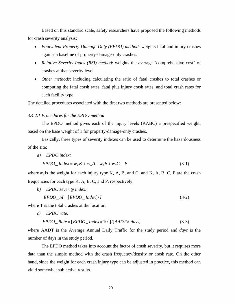
3.4.2.1 Procedures for the EPDO method

The EPDO method gives each of the injury levels (KABC) a prespecified weight,

based on the base weight of 1 for property-damage-only crashes.

Basically, three types of severity indexes can be used to determine the hazardousness

of the site:

a) EPDO index:

PCwBwAwKwIndexEPDO CBAK ++++=_ (3-1)

where is the weight for each injury type K, A, B, and C, and K, A, B, C, P are the crash

frequencies for each type K, A, B, C, and P, respectively.

wi

b) EPDO severity index:

EPDO_ SI = [EPDO_ Index]/T (3-2)

where T is the total crashes at the location.

c) EPDO rate:

EPDO_ Rate = [EPDO_ Index ×106]/[AADT × days] (3-3)

where AADT is the Average Annual Daily Traffic for the study period and days is the

number of days in the study period.

The EPDO method takes into account the factor of crash severity, but it requires more

data than the simple method with the crash frequency/density or crash rate. On the other

hand, since the weight for each crash injury type can be adjusted in practice, this method can

yield somewhat subjective results.

20

3.4.2.2 Procedures for the RSI method

The RSI method multiplies the crash frequency at each severity level by the average

"comprehensive cost" for crashes at that severity level. The subtotals for each of these

severity-specific costs are summed, and the sum is divided by the total crash frequency, as

shown in the following equation:

RSI = (C K +CA A+C B+CB CC CPP) /(K A B C P) (3-4) + + + + +K

The RSI method allows the inclusion of crash severity in screening high-crash

locations. However, like the EPDO methods, it also requires more information about each

site than the simpler methods. Additionally, the RSI method, through its use of severity cost,

introduces estimated measures into the computation rather than utilizing the data as is. If

these estimated measures are not accurate, the resulting list of priority locations will be

inaccurate.

3.4.3 Procedures for Quality Control Methods

Although all of the above methods generate useable lists for hazardous site ranking,

none of them employs any measure of statistical significance. The quality control method,

also referred to as the critical ratio method, attempts to maximize the probability that only

“truly” hazardous locations will be identified.

A statistical test based on the commonly accepted assumption that traffic crashes are

Poisson (randomly) distributed is used to determine whether the actual crash frequency, crash

density, or crash rate of a particular location is statistically higher than a predetermined

average rate of locations with similar physical characteristics. All methods in this family can

be divided into the following two categories:

a) Number Quality Control method

For each roadway category, the critical crash frequency/density is calculated based on

the average value, traffic volume, and a Poisson distribution probability constant of a desired

level of significance:

Fc = Fa + k Fa

M+

12M

(3-5)

where Fc is the critical crash frequency/density, Fa is the average crash frequency/density

within the same category, k is the level of confidence factor, and M is millions of vehicle

miles (for sections) or millions of vehicles (for interchanges).

21

b) Rate Quality Control method

The procedures of the Rate Quality Control method are very similar to those of the

Number Quality Control method. The critical crash rate is calculated using the following

equation:

Rc = Ra + k Ra

M+

12M

(3-6)

where is the critical crash rate, is the average crash rate within the same category, Rc Ra k is

the level of confidence factor, and M is millions of vehicle miles (for sections) or millions of

vehicles (for interchanges).

If the actual crash frequency/density/rate of a particular location is higher than the

critical crash frequency/density/rate for the corresponding road type, that location is

considered to have an unusually high number of crashes and is designated as a high-crash

location.

The quality control methods recognize the random nature of traffic crashes and take

into account traffic exposure in the analysis process. Also, they allow responsible agencies to

determine the priorities by grouping locations according to their functional classification.

Though these are improvements over the previous methods, they still have some notable

deficiencies.

For instance, compared with the simpler methods, the quality control methods are

quite data intensive. Additionally, the assumption that all crashes follow the Poisson

distribution has been questioned in the recent literature. The negative binomial distribution,

which assumes that the crash counts are usually more widely dispersed than would be

consistent with the Poisson assumption, has been adjudged a better representation (Hauer,

2002). Finally, the choice of which k-factor value to pick is highly subjective, giving rise to

possible ambiguity in results from year to year.

3.4.4 Composite Methods

Three composite methods have been found in the state-of-the-practice procedures: the

frequency-rate method, the weighted rank method, and the crash probability index (CPI)

method.

22

3.4.4.1 Procedures for the frequency-rate method

The frequency-rate method combines the crash frequency/crash density method and

the crash rate method. This method classifies all candidate sites as high-crash locations if

their crash frequency (or crash density) and crash rate exceed the present thresholds. The

crash frequency or crash density is used to create the initial list, and the crash rate is used to

produce the final list.

Note that some candidate sites with high crash frequencies/densities under this

method may appear to be problematic, but they may not be ranked at the hazardous level if

the traffic volumes are also high. On the other hand, sites with high crash rates due to

extremely low traffic volumes and low crash frequencies/densities may not meet the critical

values for classification as priority list locations.

3.4.4.2 Procedures for the weighted rank method

The weighted rank method combines some of the previous methods (such as crash

frequency/density, crash rate, and crash severity) in calculating a single index value for each

site. Two kinds of composite indexes are often used in the weighted rank method

(Pulugurthaa et. al., 2007):

a) Sum-of-the-rank method

SR( j) = w(i, j)× rank(i, j)i∑ (3-7)

where i is the selected method (e.g., crash frequency/crash density/crash rate/crash severity);

j is the location to be screened; w(i, j) is the weighting factor for selected method i at

location ) iis the ranked order by selected method at location rank(i, jj ; and j .

b) Crash score method

scoreCI(i, j) = CI(i, j)maxCI(i)

×100 (3-8a)

CS( j) = w(i, j)× scoreCI(i, j)i

C

∑ (3-8b)

is the actual value for selected method i at locationI(i, j) j ; and maxCIwhere (i)

i

is the

maximal value for selected method among all the locations.

Note that the weights can be adjusted in practice, based on an agency’s priorities. As

a result, the identification results from this composite index method are flexible and

23

somewhat subjective.

3.4.4.3 Procedures for the crash probability index (CPI) method

The crash probability index (CPI) method, much like the weighted rank method,

combines the information from the previous methods. As part of the CPI method, when a site

has a significantly worse than average crash frequency/density, crash rate, or severity

distribution, it is assigned penalty points. The overall CPI for a site is a summation of the

penalty points across these three measures. Its procedure can be summarized as follows:

a) If the crash frequency/density, crash rate, and the casualty ratio do not equal or

exceed their corresponding critical values, the CPI for the site is zero.

b) If the crash frequency/density equals or exceeds the corresponding critical crash

frequency/density, assign five penalty points.

c) If the crash rate equals or exceeds the corresponding critical crash rate, assign five

penalty points.

d) If the casualty ratio equals or exceeds the corresponding critical casualty ratio,

assign ten penalty points.

e) Add the sub-CPI penalty points to obtain the site CPI.

It should be mentioned that the CPI method also requires an extensive data set and

tremendous computing efforts. Additionally, adjustment of the sub-CPI penalty points can be

highly subjective.

3.5 RECOMMENDATIONS

This chapter has reviewed all methods available in the literature for ranking and

selection of hazardous locations. Their pros and cons, along with recommendations for

enhancing the procedures used in Maryland, are summarized below:

a) Using safety performance functions (SPFs) and observed crash frequency for

reliable estimation of site crash frequency — As discussed in the previous sections,

the combined use of SPF and observed crash frequency could effectively reduce

the regression to the mean problem.

b) Developing and calibrating SPFs for the State of Maryland — Instead of using the

SPFs developed by other states, it is essential that Maryland develop and calibrate

its own SPFs to better estimate crash frequency. SPFs should be developed and

24

calibrated for different types of sites and for different severity levels.

c) Using negative binomial distribution to represent the variation of crash

frequency — To better describe the usually overdispersed crash data, negative

binomial distribution, instead of Poisson distribution, should be used in the

significance tests in order to obtain a more reliable conclusion.

d) Allowing sliding windows across the adjacent road section sites — Instead of using

fixed-length sliding windows, the evaluation windows should be allowed to slide

across adjacent road section sites (i.e., one portion of the sliding window could be

in the previous section while the other is in the next section). Allowing sliding

windows to be placed across two different sections could effectively check whether

these locations experience abnormally high crash frequencies due to changes of

section characteristics that might not be easily checked by considering the two

sections separately.

e) Develop a multi-criteria system to enhance the SHA’s current procedures for

selection and ranking high-crash locations — Most existing methods for identifying

and ranking high-crash locations are based mainly on crash frequency and rate,

which are relatively straightforward but fail to truly reflect the complex interactions

between such contributing factors as crash nature, severity level, behavior of

driving populations, and geometric features. Thus, a multi-criteria system may be

desirable, as it can take into account the state-of-the-practice experience, state-of-

the-art knowledge, and currently available crash information.

25

CHAPTER 4 COST/BENEFIT ANALYSIS

4.1 INTRODUCTION

Ensuring the maximum safety for roadway users entails the design and

implementation of remedial measures for all locations identified as hazardous. However, due

to resource constraints, most responsible agencies can only implement proposed

countermeasures for a limited number of locations each year. Thus, how to effectively

compare, select, and prioritize locations for safety improvement has emerged as one of the

most critical issues for highway agencies.

To effectively compare countermeasures among all candidate locations, most state

highway agencies have employed one of the following indicators for their cost/benefit

analysis:

• Reduction in crash frequency — which measures the reduction in crashes due to

implementation of the proposed countermeasures. Using this indicator ensures

that the selected countermeasures can result in the most effective safety

improvement, not taking into account the implementation cost.

• Cost effectiveness — which reflects the cost of the countermeasure for reducing

one crash. Its advantage lies in its flexibility at assessing the trade-off between the

implementation cost and the resulting improvement. This indicator, however, fails

to account for any reduction to the severity level.

• Cost/benefit ratio and net benefit — which considers implementation costs,

benefits, and the resulting net benefits. This indicator has the strength of allowing

different benefit weights for different levels of crash severity improvement.

Over recent decades, traffic safety researchers have proposed a large body of

cost/benefit analysis methods for such a need. The remainder of this chapter will summarize

the core concepts of those methods.

4.2 MARYLAND PROCEDURES FOR COST/BENEFIT ANALYSIS

This section reviews the cost/benefit analysis method currently used by the Maryland

SHA (MDSHA, 2007a), which includes estimations of future crash frequency,

countermeasure effectiveness, and the resulting costs and benefits.

26

4.2.1 Procedures for estimating the future crash frequency

The Maryland procedure involves estimating the future crash frequency for each type

of collision for only the year of countermeasure implementation. The future crash frequency

is projected using the following simple equation:

iii VOLRATEFREQ ×= cc

c c

ccc

c

c

c

ccc

(4-1)

where is the crash frequency of collision type c; is the crash rate of collision

type c; and VOLi is the traffic volume of the study location in the year of countermeasure

implementation. Thus, the estimation of the future crash frequency is based on the estimated

crash rate and traffic volume for the future period, where the crash rate in the implementation

year, , is assumed to equal the average of the three years before the implementation.

In contrast, the estimated volume for the implementation year, VOLi, is projected with a

linear variation based on the traffic volumes for the three years preceding the implementation.

iFREQ

ciRATE

iRATE

Note that, despite the convenience of using only minimum data, the current approach

used in Maryland for estimating future crash frequencies does not consider the volume-

dependent crash rate or the nonlinear nature of traffic volume variation.

4.2.2 Procedures for estimating countermeasure effectiveness

The current Maryland procedure estimates countermeasure effectiveness in terms of

crash reduction, based on the following equation:

miim FACFREQdReFreq ×= (4-2)

where is the reduction in crash frequency for collision type c in the year of

implementation if countermeasure m is implemented; is the estimated crash

frequency of collision type c in the year of countermeasure implementation; and is the

crash reduction factor of countermeasure m in reducing collision type c.

imdReFreq

iFREQ

mFAC

Equation 4-2 allows the computation of the benefit of reducing the frequency for

collision type c due to the implementation of countermeasure m, using the following equation:

imim AccCostdReFreqFYB ×= (4-3)

where AccCostc is the average annual collision cost incurred by collision type c.

27

Most of the crash reduction factors used in the above procedure are derived from the

California Division of Highways, the Mississippi State Highway Department, and the New

York State DOT (MDSHA, 2007a); these factors may not precisely reflect the actual effects

of countermeasures for local (Maryland) driving populations.

4.2.3 Procedures for estimating costs and benefits

The current Maryland procedure uses the Equivalent Uniform Annual Cost (EUAC)

and Equivalent Uniform Annual Benefit (EUAB), which are commonly adopted in project

evaluation, to estimate costs and benefits throughout the evaluation period. The main idea of

the EUAC and EUAB is to evenly distribute all incurred costs (EUAC) and gained benefits

(EUAB) of the countermeasures, including all necessary discounts, like interest rate, over its

entire service life. For the EUAC, the Maryland procedure has included: (i) implementation

costs (i.e., all costs incurred to implement the countermeasures); (ii) operation/maintenance

costs (i.e., the annual cost incurred to operate/maintain the countermeasure); and (iii) salvage

costs (i.e., any monetary value retained after the service life of the countermeasure).

For the EUAB, the Maryland procedure includes only the benefits resulting from the

reduction in crashes due to the countermeasure implementation. More specifically, its EUAB

is evaluated from: (1) all FYBs resulting from implementation of the selected countermeasure,

(2) the interest rate used to discount the future year benefits to their present value for the

evaluation of the EUAB, and (3) the traffic volume growth rate used with the FYBs to

estimate the future benefit due to crash reduction.

Overall, the above procedures for estimating the EUAC and EUAB are relatively

simple and convenient for use by practitioners. However, they have the relatively strong

embedded assumption that a direct relationship exists between traffic volume and the

resulting benefits. Also, the hypothesis that the rate of traffic volume growth will remain

constant over the future time horizon may not be consistent with the actual patterns in some

regions.

4.2.4 Selected indicators for countermeasure comparison

Maryland’s current procedure employs the cost/benefit ratio, based on the EUAC and

EUAB, as the indicator for comparing different countermeasures. A countermeasure will be

considered potentially effective provided that its estimated cost/benefit ratio exceeds unity.

28

4.3 SAFETYANALYST PROCEDURES

This section presents the procedures for cost/benefit analysis adopted by the

SafetyAnalyst software (FHWA, 2006), including its estimation of future crash frequency,

countermeasure effectiveness, costs and benefits, and selection of indicators for comparison.


SafetyAnalyst estimates the crash frequency for a target year using an empirical

Bayesian (EB) approach (see Appendix II). Using this EB-based crash frequency,

SafetyAnalyst offers the following equation for predicting the crash frequency of year n in

the future, : nEBFREQ

nSPF

TOTSPF

TOTEBnEB FREQ

FREQFREQ

)(

)(=FREQ

n

(4-4)

where FREQEB(TOT) and FREQSPF(TOT) are, respectively, the total EB- and SPF-based crash

frequencies over years in the before period; and is the SPF-based crash frequency

of year n in the future period. This future SPF-based crash frequency is evaluated with the

same SPF but uses a constant growth factor to adjust the AADT.

SPFFREQ

Note that SafetyAnalyst estimates the crash frequencies based not only on the average

frequency for the target location but also on the SPFs calibrated with data from similar

locations. The main advantage of including SPFs in the estimation is to remove the biases

incurred by temporal fluctuations of the crash frequency data.

Equation 4-4 is grounded on the following two assumptions: (1) traffic volume for

estimating the SPF-based crash frequency will increase at a constant rate, and (2) the ratio

between the EB- and SPF-based crash frequencies will remain unchanged in the future period.

These assumptions may not be valid for use in a scenario where the period after

countermeasure implementation is relatively long.


Similar to the procedure adopted in Maryland, the SafetyAnalyst procedure employs a

crash modification factor (AMF) in estimating the crash frequency after the implementation

of countermeasures. However, with SafetyAnalyst, each crash severity level has its own

AMF that may not be a constant. For instance, the AMF for countermeasures such as

29

flattening horizontal curves and widening lanes may vary with the design characteristics. In

contrast, the countermeasure of implementing signals at intersections shall have an AMF of

constant value, as its impact on safety improvement does not depend on the given signal

design.

Based on the selected list of AMFs, SafetyAnalyst defines the benefit of reducing

crashes at severity level s in year n due to the implementation of countermeasure m as

follows:

( ) ssm

nEB

nsm AccCostAMFFREQBENE ×−×= 1 (4-6)

where AccCosts is the average cost of each crash of severity level s.

With a well-calibrated set of AMF functions, SafetyAnalyst can better estimate the

safety improvement produced by the proposed countermeasures, helping responsible

agencies to maximize the resulting implementation effectiveness. However, for those

combined countermeasures, SafetyAnalyst assumes that their individual benefits are

independent rather than interrelated, which may underestimate the actual benefits.

4.3.3 Procedures for estimating cost and benefit over the evaluation period

The SafetyAnalyst software employs the method of present value to represent the cost

and benefit of the target countermeasure over the evaluation period. Based on the

construction costs of the proposed countermeasure, SafetyAnalyst will perform its present

value method with the following two steps: (1) estimating the uniform annual construction

cost throughout the service life of the countermeasure, and (ii) computing the present values

for the uniform annual construction costs throughout the evaluation period. These two steps

could be represented with Equations 4-7 and 4-8:

( )( ) 11

1−+

+×=

m

m

S

S

mm RRRCCACC (4-7)

( )( )N

N

mm RRRACCPCC+

−+×=

111

(4-8)

where CCm, ACCm, and PCCm are, respectively, the construction cost, annual construction

cost, and present values of construction costs for countermeasure m; Sm is the service life of

30

countermeasure m; N is the duration of the evaluation period; and R is the annual rate of

return.

Compared to the cost estimation procedures used by the Maryland SHA, the method

offered by SafetyAnalyst has the following advantages: (1) it uses the present values to give

a precise cost estimation of the proposed countermeasures; and (2) it takes into account the

countermeasure service life and the evaluation period in the cost estimation. Note that

SafetyAnalyst takes only a portion of the construction costs as the cost of the proposed

countermeasure. The portion to be used depends on the length of the evaluation period N and

the service life Sm, of the proposed countermeasure. Also note that its estimation of the

present value of the benefits (PBm), based on the annual benefit ( ), can be done with

the following equation:

nsmBENE

( )∑∑= = +

=S

s

N

nn

nsm

m RBENEPB

1 1 1 (4-10)

where S is the number of different severity levels considered. This estimated present benefit

shares the same advantage discussed in previous sections: it considers the evaluation period

and service life of the proposed countermeasures.

4.3.4 Indicators for countermeasure comparison

SafetyAnalyst compares all candidate countermeasures using two different

approaches: priority ranking and criteria optimization. In priority ranking, countermeasures

will be ranked based on the following indicators: (1) cost effectiveness; (2) EPDO-based cost

effectiveness; (3) cost/benefit ratio; (4) net benefits; (5) construction costs; (6) safety benefits;

(7) total number of crashes reduced; and (8) number of fatal and injury crashes reduced. All

monetary values associated with the costs and benefits for ranking analysis are taken as the

present value so that users can then determine the countermeasure for implementation based

on the available budget and the ranked list. Some of those indicators are proposed uniquely

by SafetyAnalyst. We thus further discuss them below.

The EPDO-based cost effectiveness (i.e., the equivalent-property-damage-only-based

cost effectiveness) is similar to cost effectiveness, except that it takes the total crash reduction

as the weighted sum of reduced crashes and their severity levels. Likewise, the safety benefits

indicator is expected to be more accurate than that of the number of total crashes reduced, as

31

the crash reduction is weighted by the cost associated with each severity level. Although

using this indicator may improve estimation accuracy, the extent of improvement depends

heavily on the cost adopted for each level of crash severity. The indicator of construction

cost is not suitable for ranking and selecting countermeasures, since no measurement of

benefits (e.g., crashes reduced) is involved in the computation.

4.3.5 Procedures to maximize safety benefits under a budgetary constraint

Instead of choosing the countermeasures with the highest net benefits (or any other

evaluation indicator), SafetyAnalyst offers the following optimization approach to consider

the trade-offs between the costs and benefits of the countermeasures so that the selected

improvement schemes will maximize the total net benefit under any given budget:

∑∑=l m

lmlmZNBTBMaximize (4-10a)

Subjected. to Zlmm∑ =1 ∀l (4-10b)

PClmZlmm∑

l∑ ≤ B (4-10c)

where NBlm is the net benefit of countermeasure m implemented at location l; Zlm is the

decision variable of implementation; 1=lmZ if countermeasure m is implemented at location

l and equal to 0 if it is not implemented; PClm is the present value of the implementation cost

for implementing countermeasure m at location l; and B is the budget available for safety

improvement. Constraint 4-10b limits each location to only one countermeasure, while

constraint 4-10c ensures that the total implementation cost of the chosen countermeasure is

within the available budget.

One potential improvement for the above optimization approach would be to employ

multiple criteria — since multiple criteria are often needed in the selection and evaluation

process — and take into account their relative importance.

4.4 PROCEDURES USED BY THE STATE OF INDIANA

Several cost/benefit analyses from different states have been reviewed and compared

in the literature (Tarko and Kanodia, 2003). This section will focus on analyzing and

commenting on the cost/benefit analysis from Indiana, one of the most comprehensive

methods.

32


Similar to the use of SPF functions in SafetyAnalyst, both the observed crash

frequency and average crash frequency from similar sites are used in Indiana’s procedure for

estimating the crash frequency of the target location. Equation 4-11 presents such

formulations for computing the crash frequency of the present year, FREQInd, for any

severity:

1

10011

YZ

SPF

bObv

IndR

YrbFREQD

FREQDFREQ

×

⎟⎠⎞

⎜⎝⎛ +×

+×

+=

1

b

b

n

(4-11)

where is the observed crash frequency of the evaluated location during the before

period b; Yrb is the number of years in the before period with data used in estimation;

FREQSPF is the crash frequency estimated from the SPF for similar locations; D is the

overdispersion parameter from the calibration of the corresponding SPF; R is the average

percentage change of exposure during the before period; Y1 is the number of years between

the midpoint of the before period and the present year; and Z is a calibrated constant.

ObvFREQ

If the SPF function provides a good fit with the crash frequency of similar sites,

which gives a small value of D, the first terms of the numerator and denominator will be

dominated, and more weight will be put on the crash frequency estimated by the SPF.

Otherwise, the SPF shall yield a large value of D, and the first terms of the numerator and

denominator will approach zero. Consequently, the estimated crash frequency will depend

heavily on the observed crash frequency of the evaluated location, . By multiplying

an exposure adjustment factor (EAF) by the estimated current crash frequency (Equation 4-

10), the Indiana procedure estimates the crash frequency of year n in the future, ,

with the following equation:

ObvFREQ

IndFREQ

2

1001Ind

nInd

RFREQFREQ ⎟⎠⎞

⎜⎝⎛ +×=

YZ×

(4-12)

where Y2 is the years between the present year and year n in the future.

Like the EB approach adopted by SafetyAnalyst, the Indiana procedure uses the

observed and SPF crash frequencies to estimate the present crash frequency. Such an

33

approach could significantly reduce the potential estimation errors due to temporal

fluctuations of crash frequency at the target location.

Equations 4-12 and 4-13 assume that crash frequencies change annually by a constant

rate, ( , with a predefined change in exposure, R, and in parameter Z. This has

the advantage of introducing parameter Z to incorporate the nonlinear relationship between

the changes in crash frequency and in exposure. As the change in exposure, R, depends on

the traffic volume, which is assumed to be constant, the future crash frequency found by

Equation 4-13 may not be accurate if the target location experiences a substantial change in

traffic volume during the evaluation period.

) 1100/1 −+ ZR


The current Indiana procedure estimates countermeasure effectiveness based on the

crash reduction, evaluated from the equation below:

sm

nsInd

snm FACFREQdFreq ×=Re (4-13)

where is the reduced crash frequency of severity level s in year n after

implementing countermeasure m; is the crash frequency of severity level s of year n

after countermeasure implementation; is the crash reduction factor of countermeasure

m in reducing crashes of severity level s. By multiplying the reduced frequency of crashes

with their associated costs by different severity levels, one can estimate the resulting benefits.

If a single location has multiple improvements, the Indiana procedures suggest using a

multiplication rule (see Equation 4-14 below) to find the overall crash reduction factor on

severity level s, .

snmdFreqRe

FAC

nsIndFREQ

FAC sm

s

( )smm

s FACFAC −Π−= 100100 (4-14)

The crash reduction factors adopted in the Indiana procedures were derived from

three major sources: (1) Indiana’s own data, developed and calibrated by the state; (2) reports

from FHWA, and (3) data adopted from other states, such as Missouri, Colorado, Kansas,

California, Kentucky, Iowa, Florida, New York, and Kansas.

34

4.4.3 Procedures for estimating costs and benefits over the evaluation period

The Indiana procedure uses the EUAC and EUAB to estimate the costs and benefits

for a proposed countermeasure over the evaluation period. In computing the EUAC, the

Indiana procedure includes countermeasure implementation costs, operation/maintenance

costs, and salvage costs. For the EUAB, the Indiana procedure suggests first estimating the

reduced crash frequency for each year in the future, as discussed in the previous section, and

then computing the annual benefit with an inflation-adjusted crash cost, AccCosts, and the

following expression:

3

10010

ss FAccCostAccCost ⎟⎠⎞

⎜⎝⎛ +×=

Y

s

(4-15)

where is the crash cost for the year when the unit crash cost (Yrc0) is computed; Y3

is the number of years between the present year and Yrc0; and F is the average inflation rate

in the Y3 period.

AccCost 0

Note that, unlike Maryland and SafetyAnalyst, Indiana takes the inflation rate into

account in the cost/benefit analysis. If the inflation rate modification is neglected, the actual

unit crash cost (or benefit) may be either underestimated (if inflation occurs) or

overestimated (if deflation occurs).

4.4.4 Selection of indicators for countermeasures comparison

The Indiana procedure uses the cost/benefit ratio, based on the EUAC and EUAB

found in the previous section, as the indicator for comparison. Indiana views

countermeasures with cost/benefit ratios exceeding unity as economically beneficial for

implementation. For those with cost/benefit ratios less than one, the Indiana procedure

suggests that users take into account their secondary benefits, including several economic

benefits such as improved capacity or reduced junction delay.

Note that, with the addition of secondary benefits, more potentially beneficial

countermeasures, which may not be economically beneficial based on crash reduction alone,

could be included for the final selection. However, it should be noticed that costs and

benefits always come in pairs. One shortcoming of the current Indiana procedures is their

failure to consider the secondary costs associated with the proposed countermeasures, which

35

may create adverse impacts to nearby freeway/road systems in spite of their benefits in crash

reduction at the target intersection.

4.5 RECOMMENDATIONS

This chapter has reviewed the cost/benefit analysis methods used in the Maryland

procedure, SafetyAnalyst, and the Indiana procedure with respect to estimating: future crash

frequency, countermeasure effectiveness, the costs and benefits of countermeasures. We also

compared the selected indicators. The evaluation results suggest the following

recommendations for enhancing the current procedures used in Maryland for cost/benefit

analyses:

a) Adopt nonlinear estimations of future traffic volumes. As discussed in section

4.2.1, employing nonlinear curves to find the trend of the future volume variation

will more precisely estimate future traffic volumes over long periods.

b) Develop and calibrate crash reduction functions for the Maryland data. As the

currently used crash reduction factors are derived from other states, it is essential

for Maryland to produce those functions with its local data. For each

countermeasure type, Maryland should develop and calibrate crash reduction

functions for different severity levels, ranging from property-damage-only crashes

to fatal crashes.

c) Consider secondary costs/benefits. As discussed in section 4.4.4, the

implementation of countermeasures will reduce not only crash frequency, but also

have other impacts on the neighboring freeway/road systems. Thus, it is essential to

include secondary costs and benefits in evaluating proposed countermeasures.

d) Consider using multiple selection indicators. Different selection indicators, such as

those adopted in SafetyAnalyst (section 4.3.4), should also be considered in

performing cost/benefit analyses and comparisons of candidate countermeasures,

as each of those indicators has its own strengths and deficiencies.

36

CHAPTER 5 COUNTERMEASURE EVALUATION

5.1 INTRODUCTION

The core of the evaluation task is to compare the crash frequency and severity level of

a location after implementing the proposed countermeasures with those of the do-nothing

scenario. This differs from the cost/benefit analysis, which is based solely on the predicted

future crash frequency; performing the countermeasure evaluation requires both the collected

(current condition) and estimated (do-nothing scenario) accident information.

In general, four major issues may determine whether or not an evaluation of the

proposed countermeasures is reliable: (1) the estimated crash frequency, crash types, and

severity levels at the study location during the evaluation period under the do-nothing

scenario; (2) the regression-to-the-mean bias, which may result in either overestimating or

underestimating the efficiency of the countermeasures (crash reduction); (3) the indicators

selected for comparing different countermeasures; and (4) significance tests to confirm that

the reduced crashes are, indeed, due to the implemented measures.

The remaining sections of this chapter focus on reviewing the procedures for

countermeasure evaluation adopted by Maryland, SafetyAnalyst, and other states. It will also

include some recommendations for enhancing the current procedures used by Maryland’s

SHA in this regard.

5.2 MARYLAND PROCEDURES

This section will illustrate the countermeasure evaluation procedure currently adopted

in Maryland (MDSHA, 2001, 2002, 2006, 2007a, 2007b and 2007c) with respect to the

aforementioned four critical issues.

5.2.1 Do-nothing estimation

The purpose of the do-nothing estimation is to approximate the crash frequency/rate

at the target location if the countermeasure was not implemented. The estimated results serve

as the basis for finding the percentage change in the crash frequency/rate before and after the

implementation.

The Maryland procedure takes the crash rate for comparison so that the impact of

traffic volume on crash frequency can be removed. Similar to the estimation of future crash

37

frequency in the cost/benefit analysis, Maryland recommends taking this estimated rate

directly as the average of crash rates over the three years before the implementation. To

improve the accuracy of this estimation, Maryland procedures require estimating the crash

rates for different types of collision, such as rear-end or left-turn collisions, and different

severity levels, such as fatal or property-damage-only crashes.

The strength of Maryland’s methodology for do-nothing estimation lies in using

different crash rates for different types of collision and severity levels. Doing so allows a

better determination of whether the implemented countermeasure has reduced the crash rate

of the expected types of crash and a better assessment of whether the implemented

countermeasure has introduced any unexpected safety issues, such as increasing the crash

rate of any other crash types.

Like the procedures discussed in section 4.2, the current procedures for do-nothing

estimation have the major shortcoming of using a constant crash rate, which may not be

consistent with the nature of accidents. Besides, the consideration of only a single injury

level in the evaluation (MDSHA, 2001, 2002 and 2007c) should be enhanced to improve the

reliability of the estimation of effectiveness.

5.2.2 Regression-to-the-mean bias

As discussed in Appendix I, the regression-to-the-mean problem is mainly caused by

using the data from a short “before” period to compute the estimated crash frequency in the

“after” period. The countermeasure evaluations completed in Maryland over the past several

years (MDSHA, 2001, 2002 and 2007c) used the average of data from three before years as

the do-nothing frequency in the after period; thus, its results may suffer from the regression-

to-the-mean bias.

5.2.3 Indicators for measuring effectiveness

The current procedure in Maryland suggests using cost effectiveness, cost/benefit

ratio, and change in crash frequency as the set of indicators for evaluating the effectiveness

of the implemented countermeasures. The EUAC (identical to that discussed in section 4.2.3,

except using the actual implementation cost) and EUAB (from the do-nothing crash

frequency and the observed crash frequency during the service life of an implemented

measure) are taken as the cost and benefit for computing these indicators.

38

Note that both the cost effectiveness and cost/benefit ratio are aggregated measures of

effectiveness; they combine the effect of countermeasures for all collision types into a single

indicator to facilitate the comparison. In contrast, the Maryland procedure recommends

computing the change in crash frequency separately for each collision type, which is

expected to better measure the pros and cons of each implemented countermeasure.

5.2.4 Significance tests

As discussed in Section 5.1, significance tests determine whether the reduction in

crash frequency actually results from implementing the countermeasure rather than from

random variation. Maryland’s current procedure assumes that all crashes follow a Poisson

distribution; the significance of a reduction is determined with the standard figures shown in

Figure 5.2.

Figure 5.1 Crash reduction statistical confidence intervals (Source: MDSHA, 2007c)

The Maryland procedure takes the do-nothing crash frequency — i.e., the expected

accident frequency in Figure 5.2 — as the mean of the Poisson distribution used to represent

the variation of crash frequency. The curves in Figure 5.2 represent the relationship between

39

the do-nothing crash frequency (the expected frequency) and the percentage change that

yields the corresponding confidence level (e.g., 95%) of a candidate countermeasure.

Therefore, by considering the do-nothing crash frequency and the percentage change for each

type of collision, the significance of a selected countermeasure in reducing the crash

frequency of that collision type can be found from Figure 5.2. Note that Poisson distribution

has the distinguishing property that its mean is equal to its variance, which makes it unsuited

for use at locations with an overdispersed distribution of crash data.

5.3 PROCEDURES USED IN SAFETYANALYST

Following the same review format, this section will describe the countermeasure

evaluation procedure adopted in SafetyAnalyst software (FHWA, 2006) with respect to the

aforementioned critical issues.


In SafetyAnalyst, the crash frequency is estimated with the empirical Bayesian (EB)

approach described in section 4.3.1. Adopting the EB approach requires the estimation of the

SPF-based crash frequency for year n in the after period ( ) with the

corresponding AADT of that year and the SPF for that location. Using the SPF-based crash

frequency in the after period and the EB- and SPF-based crash frequency in the before period,

Equation 5-1 can estimate the total crash frequency for the do-nothing scenario in the after

period ( ):

nAfterSPFFREQ )(

)( AfterEBFREQ

)(

)()()(

BeforeSPF

AfterSPFBeforeEBAfterEB FREQ

FREQFREQFREQ = (5-1)

where FREQEB(Before) is the total EB-based crash frequency of the location in the before

period, which can be estimated with Equation II-1 (see Appendix II); and FREQSPF(Before) and

FREQSPF(After) are, respectively, the total SPF-based crash frequencies of the location in the

before and after periods.

Note that Equation 5-1 uses the same EB- to SPF-based crash frequency ratio from

the before period to the after period, which may yield estimation biases like those discussed

in Chapter 4.

40

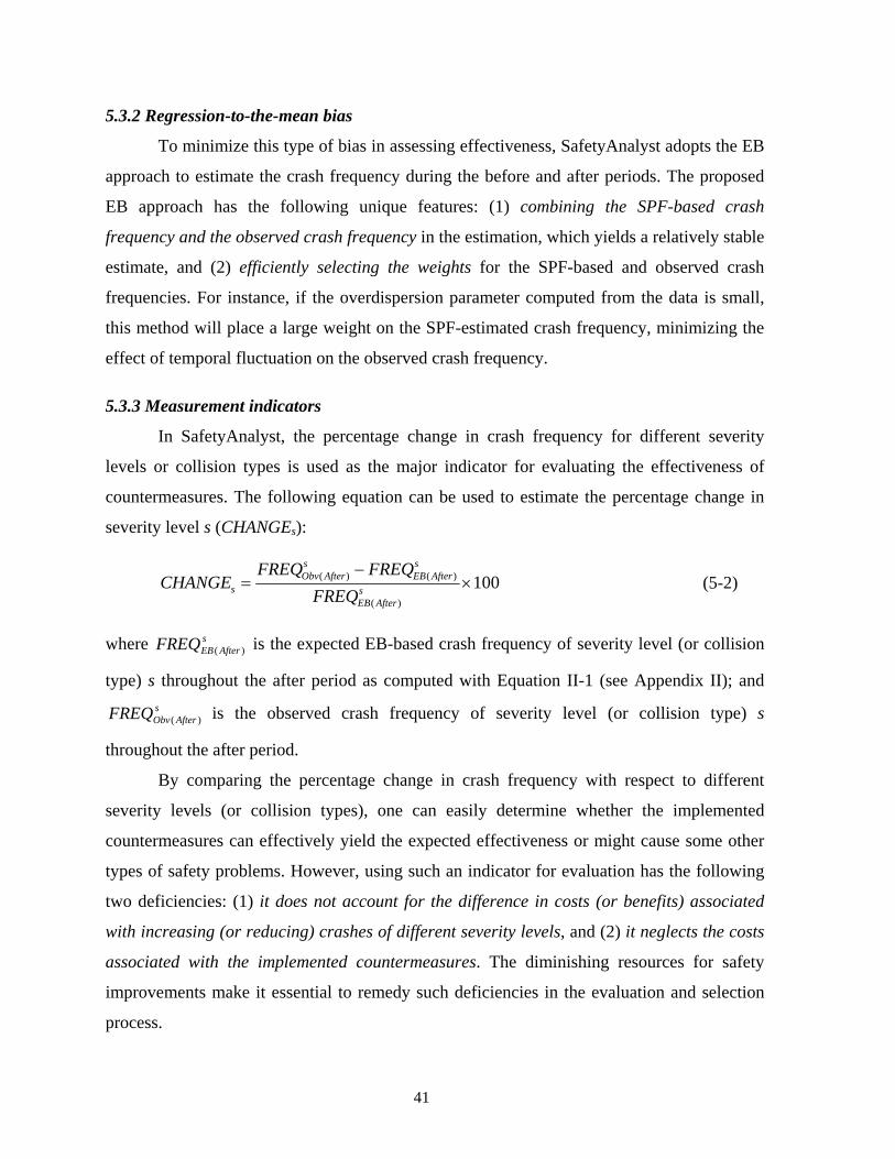
5.3.2 Regression-to-the-mean bias

To minimize this type of bias in assessing effectiveness, SafetyAnalyst adopts the EB

approach to estimate the crash frequency during the before and after periods. The proposed

EB approach has the following unique features: (1) combining the SPF-based crash

frequency and the observed crash frequency in the estimation, which yields a relatively stable

estimate, and (2) efficiently selecting the weights for the SPF-based and observed crash

frequencies. For instance, if the overdispersion parameter computed from the data is small,

this method will place a large weight on the SPF-estimated crash frequency, minimizing the

effect of temporal fluctuation on the observed crash frequency.

5.3.3 Measurement indicators

In SafetyAnalyst, the percentage change in crash frequency for different severity

levels or collision types is used as the major indicator for evaluating the effectiveness of

countermeasures. The following equation can be used to estimate the percentage change in

severity level s (CHANGEs):

100)(

)()( ×−

= sAfterEB

AfterEBAfterObvs FREQ

FREQFREQCHANGE

ss

s

(5-2)

where is the expected EB-based crash frequency of severity level (or collision

type) s throughout the after period as computed with Equation II-1 (see Appendix II); and

is the observed crash frequency of severity level (or collision type) s

throughout the after period.

AfterEBFREQ )(

sAfterObv )(FREQ

By comparing the percentage change in crash frequency with respect to different

severity levels (or collision types), one can easily determine whether the implemented

countermeasures can effectively yield the expected effectiveness or might cause some other

types of safety problems. However, using such an indicator for evaluation has the following

two deficiencies: (1) it does not account for the difference in costs (or benefits) associated

with increasing (or reducing) crashes of different severity levels, and (2) it neglects the costs

associated with the implemented countermeasures. The diminishing resources for safety

improvements make it essential to remedy such deficiencies in the evaluation and selection

process.

41

5.3.4 Significance test

The SafetyAnalyst significance test with respect to the change in crash frequency is

accomplished by employing the following index (SIGs):

( )⎟⎟⎠

⎞⎜⎜⎝

⎛=

s

ss CHANGESD

CHANGEAbsSIG (5-3)

where CHANGEs is the percentage change in crash frequency for severity level s described in

Equation 5-2; and SD(CHANGEs) is the standard deviation of CHANGEs. SafetyAnalyst

suggests that if SIG , one can conclude that the countermeasure has no effect in

changing the crash frequency at the 90 percent confidence level. On the other hand, the

countermeasures can be viewed as effective in reducing the crash frequency at the 90 percent

(or 95 percent) confidence level if (or )

7.1<

7.1≥SIG 0.2≥SIG

s

s s

The confidence level, which measures the significance of the change in crash

frequency, decreases with the value of SIGs. When the absolute value of CHANGEs decreases

to a very low level, then the observed crash frequency in the after period will be close to that

of the do-nothing scenario (Equation 5-1), which thus gives a low significance to the change

in crash frequency.

In general, an increase in SD(CHANGEs) implies that the variation of percentage

change in crash frequency is widely spread out. Hence, a large value of SD(CHANGEs) will

offset a large percentage change (CHANGEs) and yield a low significance to the change in

crash frequency. On the other hand, a large CHANGEs along with a small SD(CHANGEs)

indicates a high significance to the change in crash frequency, as it represents a scenario

which has a large crash reduction and with a high level of certainty (i.e., small variance).

Note that for SD(CHANGEs) within a reasonable range, Equation 5-3 gives a reliable

estimate of statistical significance to the change in crash frequency. However, for a very

small SD(CHANGEs), the quotient in the equation will become very large and the changes in

crash frequency will be considered as significant even with only a small percentage change

(CHANGEs). Thus, one should not rely solely on this index in determining the significance of

a crash frequency change.

42

5.4 PROCEDURES BY OTHER STATES

As before, our review of the practices by other state highway agencies will describe

only the methods used by Indiana State, which offers by far the most comprehensive and

rigorous evaluation program.


Using an approach similar to the one discussed in section 4.4.1, Indiana State

employs the following equation to estimate the crash frequency under the do-nothing

scenario, : 0IndFREQ

Z

B

A

SPF

bObv

Ind EE

YrbFREQD

FREQDFREQ ⎟⎟

⎠

⎞⎜⎜⎝

⎛×

+×

+= 1

0

1

b

(5-6)

where , , D, Yrb, and Z have the same definitions as in previous sections.

EA and EB are, respectively, the average daily exposures during the before and after periods

of the countermeasure implementation. The computation of these exposures is based on the

AADT entering the target intersection or roadway segment.

ObvFREQ SPFFREQ

The major assumption underlying Equation 5-6 is that the crash frequency, which

includes the crash frequency for the present and the do-nothing scenarios, is directly

proportional to the exposure-related factor (EA)Z only. Thus, the accuracy of the estimated

crash frequency for the do-nothing scenario could only be ensured with an updated and well-

calibrated parameter Z, which governs the nonlinear relationship between the exposure

(AADT) and the crash frequency.

5.4.2 Regression-to-the-mean problem

To minimize the effect of the regression-to-the-mean bias on countermeasure

evaluation, Indiana has developed a special method based on the observed crash frequency of

the target location and the crash frequency from the SPF of similar locations. Equation 4-12

is set up so that if the SPF is more reliable (i.e., a smaller D), the estimation will put more

weight on the SPF-estimated crash frequency. Where the SPF is less reliable (i.e., a large D),

the estimation will put more weight on the observed crash frequency of the evaluated

location. Since the method shares similar statistical properties to the EB-based estimation by

43

SafetyAnalyst, it is reasonably effective in reducing the regression-to-the-mean estimation

bias.

5.4.3 Measuring indicators

The procedures adopted by Indiana suggest using the cost/benefit ratio as the

measurement indicator for countermeasure evaluation. This ratio is computed like the EUAC

and EUAB, discussed in previous sections, but using actual rather than estimated values. For

instance, in computing the EUAB, the Indiana procedures recommend using the do-nothing

estimation results and the observed crash frequency after implementation to compute the

corresponding benefits. Note that the cost/benefit ratio is commonly used for project

evaluation; section 4.1 discusses its strengths and deficiencies.

The cost/benefit ratio used in the Indiana procedure, an aggregated measure of

effectiveness, represents the overall effect of the countermeasure on reducing crashes of

different severity levels. Although it allows a direct comparison of the effectiveness of

different countermeasures, it is difficult for the responsible agencies to tell whether the

implemented countermeasure has any adverse effect on any particular crash severity level or

collision type.

5.4.4 Significance tests

The significance test adopted by the Indiana procedures is the same as Maryland’s,

except that it uses a negative binomial (instead of Poisson) distribution in describing crash

frequencies. Note that a negative binomial distribution is generally suited for representing

overdispersed crash data that having a mean value differs significantly from the variance.

Depending on the spatial pattern of crash data, using such a distribution for statistical test

may or may not yield better results than the Poisson assumption.

5.5 RECOMMENDATIONS

The above review results suggest the following enhancements to the procedures

currently used by the Maryland SHA:

a) Using SPFs and observed crash frequency for reliable estimation of site-specific

crash frequency — Combining the use of SPFs and observed crash frequency may

yield a more reliable estimate of crash frequency for countermeasure evaluation.

44

b) Exploring the use of negative binomial distribution in the significance test — This

would ensure that some overdispersed crash data can be fitted with a proper

distribution.

c) Using SPFs of the after period in estimating the do-nothing crash frequency —

Using an approach similar to SafetyAnalyst would reduce the regression-to-the-

mean problem on do-nothing estimations.

d) Including both aggregated and disaggregated evaluation indicators — This would

enhance the evaluation quality and reliability with all available data, including both

the aggregated (i.e., cost/benefit ratio, cost effectiveness, and net benefit) and

disaggregated (i.e., percentage change in crash frequency for different severity

levels) indicators.

45

CHAPTER 6 CONCLUSIONS AND RECOMMENDATIONS

6.1 SUMMARY OF RESEARCH FINDINGS

This study offers a comprehensive review of the safety improvement programs

adopted by Maryland, FHWA (SafetyAnalyst), and other state agencies, focusing mainly on

the following imperative issues: (1) screening and ranking high-crash locations, (2)

prioritizing cost-effective projects for safety improvement; and (3) conducting before/after

studies for project implementation plans.

Based on the results of this review, we recommend that the following enhancements

be incorporated into the existing safety improvement program in Maryland:

- Develop a multi-criteria method to enhance the current procedures used by the

Maryland SHA to select and rank high-crash locations: Most existing methods for

identifying and ranking high-crash locations are based mainly on either the crash frequency

or rate, which are relatively straightforward but fail to truly reflect the complex interactions

between contributing factors such as the crash nature, the severity level, the behavior of

driving populations, and geometric features. Thus, it is essential that a multicriteria

evaluation system be adopted to incorporate the state-of-practice experience and state-of-art

knowledge from various available sources.

- Using SPFs and the observed crash frequency to reliably estimate the site-specific

crash frequency: The combined use of SPFs and the observed crash frequency could

effectively reduce the regression-to-the-mean bias at all levels of estimation. Further studies

should be carried out to determine whether Maryland should develop its own approach or just

follow the EB-based approach suggested by SafetyAnalyst.

- Developing and calibrating SPFs for Maryland: Instead of using the SPFs

developed by other states, Maryland should develop and calibrate its own SPFs to improve

estimations of crash frequency.

- Using negative binomial distribution to represent the variation of crash frequency:

Due to the mostly overdispersed crash data, Maryland should explore the use of the negative

binomial distribution, instead of Poisson distribution, in significance tests of countermeasure

effectiveness.

46

- Allowing sliding windows across adjacent road section sites: Instead of using a

fixed-length sliding window to identify hazardous locations, Maryland should allow

evaluation windows to slide across adjacent road section sites, which would effectively check

whether the target locations experience abnormally high crash frequencies due to changes of

geometric characteristics.

- Employing nonlinear estimation for future traffic volume: As traffic volume does

often not increase at a constant rate, it is essential to use a nonlinear model to project its

evolution trend with historical data.

- Developing and calibrating the crash reduction functions with local data: The set of

crash reduction factors currently used in Maryland come from other states; these functions

may not precisely reflect the change in crash frequency after countermeasure

implementation. To be effective, Maryland should calibrate a crash reduction function for

each crash type and severity level, ranging from property-damage-only to fatal crashes.

- Including secondary costs/benefits in the evaluation: As discussed in section 4.4, the

implementation of countermeasures may not only reduce crash frequency, but also result in

other impacts on the entire freeway/road system. This makes it essential to include all such

secondary benefits or costs in the process of ranking and selection projects.

- Applying a benefit-maximizing selection approach: Because the available budget for

safety improvements is always limited, Maryland should explore the trade-offs between costs

and benefits among candidate countermeasures, selecting the set that can maximize the

overall benefit.

- Exploring the use of different selection indicators: Maryland should also explore

different selection indicators, such as those adopted in SafetyAnalyst (section 4.3.4), to

ensure that all hazardous locations can be effectively identified and that the most effective

countermeasures can be implemented.

- Using SPFs of the after period in estimating do-nothing crash frequency: To

minimize the regression-to-the-mean bias, Maryland’s procedure for estimating the crash

frequency for the do-nothing scenario should follow the approach in SafetyAnalyst.

6.2 CONCLUSION

Over the past two decades, both FHWA and state agencies have jointly devoted tremendous

resources in developing a comprehensive safety improvement program that has been

47

48

incorporated into the SafetyAnalyst software. SafetyAnalyst includes both a methodology to

guide users in identifying hazardous locations and a set of computerized tools to facilitate

project implementation. Much valuable data and many lessons are also available from the

SafetyAnalyst documentation, which may offer some effective suggestions for the Maryland

SHA to enhance its current safety program, as well as some of its analysis procedures. Hence,

it is imperative for responsible staff in the Maryland SHA to take full advantage of all

information and tools available in SafetyAnalyst and to upgrade its existing procedures under

the available resources and data constraints.

REFERENCES

1. Dixon, K. and Monsere C., 2007. Evaluating the Effectiveness of the Safety

Investment Program (SIP) Policies for Oregon-Literature Review. Technical Report.

2. Federal Highway Administration (FHWA),

2008. http://safety.fhwa.dot.gov/hsip/fivepercent/, accessed March 15, 2008.

3. Federal Highway Administration (FHWA), 2006. SafetyAnalyst User’s Manual.

4. Hauer E., 2007. Detection of Safety Deterioration in a Series of Accident Counts

Transportation Research Record 1542, pp. 38-43.

5. Hauer, E., Harwood, D. W., Council, F. M., and Griffith M. S., 2002. Estimating

Safety by the Empirical Bayesian Method: A Tutorial. Transportation Research

Record 1784, pp. 126-131.

6. Maryland State Highway Administration (MDSHA), 2001. Continuous Shoulder

Rumble Strips (CSRS) on Maryland Highways. Technical Report.

7. Maryland State Highway Administration (MDSHA), 2002. Evaluation Maryland’s

Accident Experience at Location having Red Light Running Detection Cameras.

Technical Report.

8. Maryland State Highway Administration (MDSHA), 2006. PTSWF Warning Sign

Study: Before & After Study Overview and Results. Technical Report.

9. Maryland State Highway Administration (MDSHA), 2007a. Maryland’s Highway

Safety Improvement Program: Annual Report Fiscal Year 2007. Technical Report.

10. Maryland State Highway Administration (MDSHA), 2007b. Safety Evaluation of

Red-Light Cameras in Maryland. Technical Report.

11. Maryland State Highway Administration (MDSHA), 2007c. Maryland’s

Roundabouts: Accident Experience and Economic Evaluation. Technical Report.

12. Midwest Research Institute (MRI), 2002. SafetyAnalyst: Software Tools for Safety

Management of Specific Highway Sites (White Paper for Module 1—Network

Screening). Technical Report.

49

http://safety.fhwa.dot.gov/hsip/fivepercent/

13. Pawlovich, M. D., 2007. Safety Improvement Candidate Location (SICL) Methods.

Technical Report.

14. Pulugurthaa S. S., Krishnakumarb V. K., and Nambisanc. S. S, 2007. New methods to

identify and rank high pedestrian crash zones: An illustration. Accident Analysis &

Prevention. 39(4), pp. 800-811

15. Robert K. Seyfried, 2008. Introduction to Crash Analysis. ITE Training Course.

16. Tarko, A.P. and Kanodia, M., 2003. Hazard Elimination Program – Manual on

Improving Safety of Indiana Road Intersections and Sections (FHWA/IN/JTRP-

2003/19). Technical Report.

17. United States Government Accountability Office (GAO), 2008. Highway Safety

Improvement Program: Further Efforts Needed to Address Data Limitations and

Better Align Funding with States’ Top Safety Priorities. Technical Report.

50

APPENDIX- I: THE REGRESSION-TO-THE-MEAN PROBLEM

Short term average

Long term average

Actual average frequency without improvement

Actual reduction

Estimated reduction

Improvement implementation Estimated average based on

short term observed data

3-year average after improvement

Crash frequency

Year

Figure I.1 Regression-to-the-mean

In Figure I.1, the vertical dotted line represents the time during which the

countermeasure is implemented. The left of this dotted line shows the variation of crash

frequencies at this location before implementation of the countermeasure. Due to the

availability of data, most screening methods can only use the short-term average to identify

high-crash locations. On the right of the vertical dotted line shows the variation of crash

frequencies after countermeasure implementation. The three horizontal lines on the right side

respectively (from the top) represent the average crash frequency estimated from the previous

short-term average, actual average crash frequency without improvement, and the average

crash frequency after the improvement.

Note that the actual average crash frequency without improvement is assumed to be

known in this figure for convenience of illustrating the nature of the regression-to-the-mean

problem. Comparing to the short-term average before the countermeasure implementation,

51

52

the average crash frequency without improvement should fall back to a level close to the

long-term average. This is due to the fact that such a high crash frequency before the

improvement is only a short-term fluctuation, and the crash frequency (given that all other

parameters, such as traffic volumes, remain unchanged) will finally “regress” back to the

long-term average. If the crash frequency for the do-nothing scenario is estimated solely on

the short-term average, the estimated reduction will be larger than the actual number, and

thus result in overestimate of the effectiveness of the countermeasures. Some locations

experiencing short-term low crash frequencies (compared to their long term averages) will

also have the same regression-to-the-mean problem, which would be an underestimate of

their countermeasure effectiveness.

APPENDIX- II: THE EMPIRICAL BAYESIAN (EB) APPROACH

The EB-based crash frequency is presented below to clarify the explanations and

comments made in this report:

( ) lsObv

lsSPF

lsEB FREQwFREQwFREQ ×−+×= 1 (II-1)

where, , and are respectively the EB-based, SPF-based and

observed crash frequencies for severity level s at location l; w is the weight of SPF-based crash

frequency for estimating the EB-based crash frequency. The EB approach uses two different

pieces of crash information (shown in Figure II.1): (1) crash frequencies of locations that are

similar to the study location (first term in the right-hand side of equation II-1) and; 2) observed

crash frequency of the study location (second term in the right-hand side of equation II-1), for

making an accurate estimation of the crash frequency.

lsEBFREQ ls

SPFFREQ lsObvFREQ

The EB approach can achieve an accurate estimation by choosing the proper weight w in

equation II-1. SafetyAnalyst defines the weight w with the following equation:

lBeforeSPFFREQd

w)(1

1×+

= (II-2)

where is the sum of the SFP-based crash frequencies for location l throughout the

before period; d is a measure of dispersion for the crash frequencies of the locations used for

calibrating the SPF. If locations with a dispersed distribution of crash frequencies are used in the

SPF calibration, the parameter d will have a large value and thus yield a small weight w. Hence,

to estimate the EB-based crash frequency with equation II-1, one needs to put more weight on

the observed crash frequency of the study location. On the other hand, it is necessary to place

more weight on the SPF-based crash frequency to estimate the EB-based crash frequency if the

variance of crash frequencies for those locations used in the SPF calibration is small (i.e. a

smaller over-dispersion parameter).

lBeforeSPFFREQ )(

53

54

Volume

Crash frequency

SPF

EB-based crash frequencies Observed crash frequencies

SPF-based crash frequencies

Figure II.1 EB-based, SPF-based and observed crash frequencies

Review and Enhancement for Crash Analysis and Prediction ...

Documents

Transcript of Review and Enhancement for Crash Analysis and Prediction ...