ISIJ International, Vol. 39 (1999), No. 10, pp, 966-979

ReviewNeural Networks in Materials Science

H. K. D. H BHADESHIAUniversity of Cambridge, Department of Materials Science and Metallurgy,E-mail: hkdb@cus.cam.ac.uk www,msm.cam,ac,uk/phase-trans

(Received on April 2. 1999, accepted in final form on June 12.

PembrokeStreet, CambridgeCB23aZ,

1999)

UK.

There are difficult problems in materials science where the generai concepts might be understood butwhich are not as yet amenableto scientific treatment. Weare at the sametime told that good engineeringhas the responsibility to reach objectives in a cost and time-effective way. Any model which deals withonly a smali part of the required technology is therefore unlikely to be treated with respect. Neural networkanalysis is a form of regression or classification modelling which can help resolve these difficulties whilststriving for longer term solutions. This paper begins with an introduction to neural networks and contains

a review of someapp]ications of the technique in the context of materia]s science.

KEYWORDS:neural networks; materials science; introduction; applications.

1. Introduction

The development and processing of materials is

complex. Although scientific investigations on materialshave helped greatly in understanding the underlyingphenomena,there remain manyproblems where quan-titative treatments are dismally lacking. For example,whereas dislocation theory can be used to estimate theyield strength of a microstructure, it is not yet possibleto predict the strain hardening coefficient of an engi-neering alloy. It follows that the tensile strength,elongation, fatigue life, creep life and toughness, all ofwhich are vital engineering design parameters, cannoteven be estimated using dislocation theory. A morecomprehensive list of what needs to be done in this

context is presented in Table 1.

The lack of progress in predicting mechanical prop-erties is because of their dependenceon large num-bers of variables, Nevertheless, there are clear patternswhich experienced metallurgists recognise and under-stand. For example, it is well understood that the tough-ness of a steel can be improved by making its micro-structure more chaotic so that propagating cracks arefrequently deflected. It is not clear exactly howmuchthe toughness is expected to improve, but the qualitativerelationship is well established on the basis of a vastnumberof experiments.

NeLu'a] network models are extremely useful in suchcircumstances, not only in the study of mechanicalproperties but wherever the complexity of the problemis overwhelming from a fundamental perspective andwhere simplification is unacceptable. The purpose ofthis review is to explain how vague ideas might beincorporated into quantitative models using the neuralnetwork methodology. Webegin with an introductionto the method, followed by a review of its application

to materials.

2. Physical and Empirical Models

A good theory must satisfy at least two criteria. It

must describe a large class of observations with fewarbitrary parameters. Andsecondly, it must makepre-dictions which can be verified or disproved. Physicalmodels, such as the crystallographic theory of martens-ite,1'2) satisfy both of these requirements. Thus, it is

possible to predict the habit plane, orientation rela-

tionship and shape deformation of martensite with aprecision greater than that of most experimental tech-niques, from a knowledge of just the crystal structuresof the parent and product phases. By contrast, a linearregression equation requires at least as manyparame-

Table l. Mechanical properties that need to be expressedin quantitative models as a function of large

numbersof variables.

Property

Yleld strength

Ultimate tenslle strength

YS/UTSratio

Elongation

Uniform elongation

Non-uniform elongation

Toughness

Fatigue

Stress corroslon

Creep st,rength

Creep ductlllty

Creep-f atigue

Elastic modulus

Thermal expansivity

Hardncss

Relevance

All structural applications

All structural applications

Tolerance to plastic overload

Reslstance to brittle fracture

~elated to YSand UTSRelated to inclusions

Tolerance to defects

Cyclic loading, Iife assessments

Slow corrosion &cracking

Hlgh temperature service

Safe design

Fatigue at creep temperatures

Deflection, stored energy

Thermal fatigue/strcss/shock

Tribological propertics

C 1999 ISIJ 966

ISIJ Internationa[, Vol.

ters as the numberof variables to describe the experi-

mental data, and the equation itself maynot be physi-cally justified. Neural networks fall in this second cat-

egory of empirical models; we shall see that they haveconsiderable advantages over linear regression. In spite

of the large numberof parameters usually necessary todefine a trained network, they are useful in circumstanceswhere physical models do not exist.

3. Linear Regression

Most scientists are familiar with regression analysis

wheredata are best-fitted to a specified relationship whichis usually linear. The result is an equation in which eachof the inputs xj is multiplied by a weight wj; the sumofall such products and a constant ethen gives an estimateof the output y=~jwjxj +e. As an example, the tem-perature at which the bainite reaction starts (i.e. Bs) in

steel maybe written3)'

Bs('C) =830 - 270x cc ~90x cM*- 37 x cNi - 70 x cc* ~83 x cM~

o ,*,c *+'~* }*'~**+,''+*,""

.(1)

where ci is the wto/o of element i which is in solid so-lution in austenite. The term wi is then the best-fit valueof the weight by which the concentration is multiplied;

eis a constant. Becausethe variables are assumedto beindependent, this equation can be stated to apply for theconcentration range:

Carbon O.1-0.55wt"/o Nickel 0.0-5.0Silicon O. I-O. 35 Chromium O.0-3

. 5Manganese 0.21.7 Molybdenum 0.0-1.0

and for this range the bainite-start temperature can beestimated with 90 o/* confidence to + 25'C.

Equation (1) assumesthat there is a linear dependenceof Bs on concentration.* It mayalso be argued that thereis an interaction betweencarbon and molybdenumsince

the latter is a strong carbide forming element. This canbe expressed by introducing an additional term as fol-

lows:

Bs'C=830- 270 x cc~90 x cM~- 37 x cNi - 70 > cc.

- 83 x cM.+22 x (cc X cM~).(2)

interaction

Of course, there is no justification for the choice of the

particular form of relationship. This andother difficulties

associated with ordinary linear regression analysis canbe summarisedas follows:

Difficulty (a) A relationship has to be chosen beforeanalysis.

Difficulty (b) The relationship chosen tends to belinear, or with non-linear terms addedtogether to form a psued0-1inear equa-tion.

Difficulty (c) The regression equation, once derived,

39 (1999), No. 10

•\~rOf:i

hjdden unit

(1)\w(M1~~/

owc

~

Nl input nodes

\(1)tanh(~wj xj +e(1))

Ooutput node

~(a) (b)

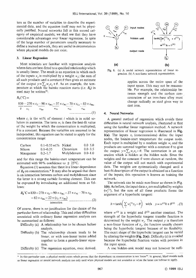
Fig. 1. (a) A neulal network representation of linear re-

gression. (b) A non-linear network representation.

applies across the entire span of theinput space. This maynot be reasona-ble. For example, the relationship be-

tween strength and the carbon con-centration of an iron-base alloy mustchange radically as steel gives way to

cast iron.

4. Neural Networks

A general method of regression which avoids thesedifficulties is neural network analysis, illustrated at first

using the familiar linear regression method. A networkrepresentation of linear regression is illustrated in Fig.l(a). The inputs xi (concentrations) define the inputnodes, the bainite-start temperature the output node.Each input is multiplied by a randomweight wi and theproducts are summedtogether with a constant eto givethe output y=~iT4;ixi+0. The summation is an op-eration which is hidden at the hidden node. Since the

weights and the constant Owere chosen at random, thevalue of the output will not match with experimentaldata. The weights are systematically changed until abest-fit description of the output is obtained as a functionof the inputs; this operation is knownas training the

network.Thenetwork can be madenon-linear as shownin Fig.

l(b). Asbefore, the input data xj are multiplied by weights(w(1)), but the sum of all these products forms the

argument of a hyperbolic tangent:

(h=tanh~~, w(1)xJ+e =with y w(2)h+0(2) (3)

where T4'(2) is a weight and O(2) another constant. Thestrength of the hyperbolic tangent transfer function is

determined by the weight T4'j. The output y is therefore

a non-linear function of xj, the function usually chosenbeing the hyperbolic tangent because of its flexibility.

Theexact shape of the hyperbolic tangent can be varied

by altering the weights (Fig. 2(a)). Difficulty (c) is avoidedbecause the hyperb•olic function varies with position in

the input space.

A one hidden-unit model maynot however be suffi-

* In this particular case, a physical model exists which proves that the dependenceon concentration is not linear4). In general, blind models such

as linear regression or neural network analysis are only used whenphysical models are not available or whenthe latter are tedious to apply.

967 C 1999 ISIJ

ISIJ International, Vol. 39 (1 999), No. 10

y

(a)

1

\2 (b)

f{xj }Fig. 2. (a) Three different hyperbolic tangent functions; the

"strength" of each depends on the weights. (b) Acombination of two hyperbolic tangents to produce amorecomplex model.

Fig. 3.

Ni input nodes

hidden units

~ OUtput node

The structure of a two hidden-unit neuralDetails have been omitted for simplicity.

network.

>, ;b

o 2 4

x

6 8 o

x

8

:b

oUJ

Fig. 4.

8 Complexity of model

Variations in the test and training errors as a function of modelcomplexity, for noisy data in a case whereyshould vary with x3. The filled points were used to create the models (i.e, they represent training data), andthe circles constitute the test data. (a) A Iinear function which is too simple. (b) Acubic polynomial with

optimumrepresentation of both the training and test data. (c) A fifth order polynomial which generalises

poorly. (d) Schematic illustration of the variation in the test and training errors as a function of the modelcomplexity.

ciently fiexible. Further degrees of non-linearlty can beintroduced by combining several of the hyperbolic

tangents (Fig. 2(b)), permitting the neural networkmethod to capture almost arbltrarily non-linear rela-

tionships. The numberof tanh functions is the numberof hidden Lmits; the structure of a two hidden unit

network is shownin Fig. 3.

The function for a network with i hidden units is

given by

y" =~T,,(2)h +e(2) ..........(4)

where

~ '

(JJ s

hi= tanh lv(~))c +e(i)

iJ.(5)

Notice that the complexity of the function is related to

the numberof hidden units. The availability of a suf-

ficiently complex and fiexible function meansthat the

analysis is not as restricted as in linear regression where

the form of the equation has to be specified before theanalysis.

The neural network can capture interactions betweenthe inputs because the hidden units are nonlinear. Thenature of these interactions is implicit in the values ofthe weights, but the weights maynot always be easy tointerpret. For example, there mayexist more than just

pairwise interactions, in which case the problem becomesdifficult to visualise from an examination of the weights.

Abetter methodis to actually use the network to makepredictions and to see how these depend on various

combinations of inputs.

5. Overfitting

A potential difficulty with the use of powerful non-linear regression methods is the possibility of overfitting

data. To avoid this difficulty, the experimental data

can be divided into two sets, a training dataset and

a test dataset. The model is produced using only the

training data. The test data are then used to check that

C 1999 ISIJ 968

ISIJ International, Vol.

the model behaves itself whenpresented with previous-ly unseendata. This is illustrated in Fig. 4. which showsthree attempts at modelling noisy data for a case where

y should vary with x3. A Ilnear model (Fig. 4(a)) is toosimple and does not capture the real complexity in the

data. An overcomplex function such as that lllustrated

in Fig. 4(c) accurately models the training data but gen-eralises badly. The optimummodel is illustrated in Fig.

4(b). The training and test errors are shownschemati-cally in Fig. 4(d); not surprlsingly, the training errortends to decrease continuously as the model complexityincreases. It is the minimumin the test error whichenables that model to be chosen which generaiises best

to unseen data.

This discussion of overfitting is rather brief becausethe problem does not simply involve the minimisationof test error. There are other parameters which controlthe complexity, which are adjusted automatically to try

to achieve the rlght complexlty of model.s,6)

Error EstimatesThe input parameters are generally assumedin the

analysis to be precise and it is normal to calculate anoverall error by comparing the predicted values Cyj) ofthe output against those measured(tj), for example,

EDCC~(tj-yj)2.........

..........(6)

EDis expected to Increase if important input variables

have beenexcluded from the analysis. WhereasEDgives

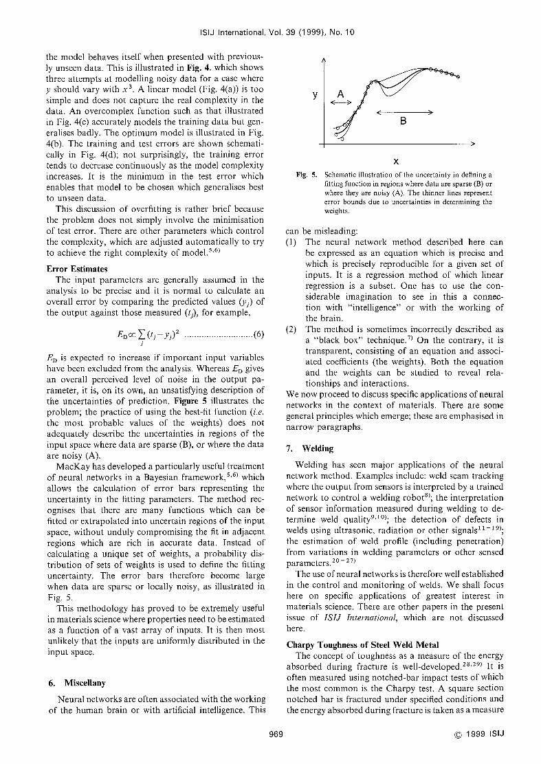
an overall perceived level of noise in the output pa-rameter, it is, on its own, an unsatisfying description ofthe uncertainties of prediction. Figure 5 illustrates the

problem; the practice of using the best-fit function (i.e.

the most probable values of the weights) does notadequately describe the uncertainties in regions of the

input space wheredata are sparse (B), or where the data

are noisy (A).

MacKayhas developed a particularly useful treatmentof neural networks in a Bayesian framework,5,6) whichallows the calculation of error bars representing the

uncertainty in the fitting parameters. The method rec-

ognises that there are many functions which can befitted or extrapolated into uncertain regions of the input

space, wlthout unduly compromising the fit in adjacentreglons which are rich in accurate data. Instead ofcalculating a unique set of weights, a probability dis-

tribution of sets of weights is used to define the fitting

uncertainty. The error bars therefore become large

whendata are sparse or locally noisy, as illustrated in

Fig. 5.

This methodology has proved to be extremely useful

in materials science whereproperties need to be estimated

as a function of a vast array of inputs. It is then mostunlikely that the inputs are uniformly distributed in the

input space.

6. Miscellany

Neural networks are often associated with the workingof the humanbrain or with artificial intelligence. This

39 (1999),

y

No. 10

A

B

969

XFig. 5. Schematic illustration of the uncertainty in defining a

fitting function in regions wheredata are sparse (B) orwhere they are noisy (A). The thinner lines represent

error bounds due to uncertainties in determining the

weights.

can be misleading:(1) The neural network method described here can

be expressed as an equation which is precise andwhich is precisely reproducible for a given set ofinputs. It is a regression method of which linear

regression is a subset. Onehas to use the con-siderable imagination to see in this a connec-tion with "intelligence" or with the working ofthe brain.

(2) The method is sometimes incorrectly described as

a "black box" technlque.7) On the contrary, it is

transparent, consisting of an equation and associ-

ated coefficients (the weights). Both the equationand the weights can be studied to reveal rela-

tionships and interactions.

Wenowproceed to discuss specific applications of neuralnetworks in the context of materials. There are somegeneral principles which emerge; these are emphasisedin

narrow paragraphs.

7. Welding

We]ding has seen major applications of the neuralnetwork method. Examplesinclude: weld seamtracking

where the oLutput from sensors is interpreted by a trained

network to control a welding robot8); the interpretation

of sensor information measuredduring welding to de-

termine weld quality9'10); the detection of defects in

welds using ultrasonic, radiation or other signalsll ~ 19)'

the estimation of weld profile (including penetration)

from varlations in welding parameters or other sensed

parameters. 20 - 27)

Theuse of neural networks is therefore well establishedin the control and monitoring of welds. Weshall focushere on specific applications of greatest interest in

materials science. There are other papers in the presentissue of ISIJ Intel'national, which are not discussedhere.

Charpy Toughnessof Steel WeldMetalThe concept of toughness as a measureof the energy

absorbed durlng fracture is weli-developed.28,29) It is

often measuredusing notched-bar impact tests of whichthe most commonis the Charpy test. A square section

notched bar is fractured under specified conditions andthe energy absorbedduring fracture is taken as a measure

C 1999 ISIJ

ISIJ International, Vol. 39 (1999), No. 10

~I

caE

O'~5

0.8

0.6

0.4

0.2

0.0

J::,~o~~o;~

Fig. 6. Bar chart showing a measureof the model-perceivedsignificance of eachof the input variables in influencing

toughness.30].

of toughness. The Charpy test is empirical in that the

data cannot be used directly in engineering design. It

does not provide the most searching mechanical con-ditions. The sample has a notch, but this is less thanthe atomically sharp brittle crack. Although the test

involves impact loading, there is a requirement to start

a brittle crack from rest at the tip of the notch, suggest-ing that the test is optimistic in its comparison against apropagating brittle crack.29) Most materials can be as-

sumedto contain sub-critical cracks so that the initia-

tion of a crack seemsseldom to be an issuc.

The Charpy test is nevertheless a vital quality con-trol measurewhich is specified widely in international

standards, and in the ranking of samples in research

and development exercises. It is the most commonfirst

assessmentof toughness and in this sense has a provenrecord of reliability. The test is usually carried out at avariety of temperatures in order to characterlse theductilebrittle transition intrinsic to body-centred cubicmetals with their large Peierls barriers to dislocation

motion.The toughness of ferritic steel welds has been studied

using neural networks.30) The Charpy toughness wasexpressed as a function of the welding process (manualmetal arc or submergedarc), the chemical composition(C, Mn, Si. Al, P, S, O&N), the test temperature andthe microstructure (primary, secondary, allotriomorphicferrite, Widmanstatten ferrite, and acicular ferrite). Theinclusion of microstructure greatly limited the quantityof data available for analysis because few such results

are reported in the literature. Nevertheless, the aim ofthe analysis was to see if the network recognised knowntrends in toughness as a function of the microstructure.

Thewelding process wasnumerically distinguished in theanalysis by using Oand I for the manualand submergedarc methods.

Figure 6Illustrates the significance ((T~) of each of theinput variables, as perceived by the neural network, in

influencing the toughness of the weld. As expected, the

welding-process has its ownlarge effect; it is well knownthat submerged arc welds are in general of a lowerquality than manua]metal arc welds. The yield strength

has a major effect; it is knownthat an increase in theyield strength frequently leads to a deterioration in the

toughness. It is also widely believed, as seen in Fig. 6,

eo'o

~ 0.5/::

t~!~

o~l 0.01:!a)~D

~c:f

~~ -0.5

~-1.0

233 K

\.

C 1999 ISIJ

Fig. 7.

O 500 1000Oxygen/ p.p,m.

Variation in the normalised toughness as a functionof the oxygen concentration. Oxygen is varied here

without changing any of the other inputs. The max-imumoxygen concentration in the training data was821 p,p.m.

970

that acicular ferrite greatly infiuences toughness, Ni-

trogen has a large effect, as is well estab]ished experi-

mentally.

A trained neural network is assoclated with reveal-

ing parameters other than just the transfer functionand weights. For example, the extent to which eachinput explains variations in the output parametercan easily be examined.

It is surprising that carbon has such a small effect

(Fig. 6), but what the results really demonstrate is that

the influence of carbon comesin via the strength andmicrostructure. Other trends have been discussed in Ref.30).

OxygenInfluences welds in both beneficial andharmful

ways, e.g. by helping the nucleation of acicular ferrite

or contributing to fracture by nucleating oxides. Thepredicted effect of oxygen concentration is illustrated in

Fig. 7a]ong with the ~I standard deviation predicted

error bars. It is clear that extrapolation into regions wheredata are sparse or noisy is identified with large error bars.

The training data used for the toughness model had amaximumoxygenconcentration of 821parts per million.

Neural network models which indicate appropri-ately large error bars in regions of the input spacewhere the fitting is uncertain are less dangerous in

applications than those which simply identify aglobal level of noise in the output.

Figure 8showshowthe toughness varies as a functionof the manganeseconcentration and the test temperature,It is obvious that the effect of temperature is smaller at

large concentrations of manganese, i,e, there is aninteraction between the manganeseand temperature.Thls interaction has been recognlsed naturally by the

model and is expected from a metallurgical point ofview,30)

ISIJ International, Vol.

Neural networks deduce the relationship betweenvariables, including any interactions. In complexcases involving manyvariables, the interactions

are revealed both qualitatively and quantitatively

by exarnining the predictions, as illustrated in Fig. 8.

Analyses carried out without an examination of the

consequenceshave tended to lead to the incorrect con-clusion that the neural network method lacks trans-

parency. For example, Chanet al.3 i) created a model for

the hardness of the heat affected zone of steel welds as

a function of the carbon concentration, the carbon-equivalent and the cooling rate within a specified tem-perature range. Having produced the model, they did notcontinue to study how the hardness depends on eachof the input parameters, whether the relationship differs

U,D,,,

,:,

EOZ~a,

,~

=O,~

O

:o

o=o,:I

Oh>~~O

Fig.

39 (1 999). No. IO

for low and high carbon steels, etc.

The toughness model described above30) js revealingbut nevertheless, Impractical for routine use because theinputs include the microstructure, which can be difficult

to predict or measure. This can be resolved by eliminatingthe microstructural inputs and including the weldingconditions (current, voltage, speed, interpass tempera-ture, arc efficiency) which determine the cooling rate ofthe weld. Themicrostructure is a function of the coolingrate and chemical composition (both easy to measure)so it does not have to be included explicitly.

For practical applications, the most useful neuralnetwork models are those whoseinputs are easily

measured, perhaps as a part of the quality control

process. Onthe other hand, it maybe revealing to

use inputs which are related directly to the outputparameter, so that mechanisms are revealed.

0.6

0,4Strength of Steel Welds

The tensile strength of a weld metal is frequently set0.2 higher than that of the corresponding base metal.32) It' 0,5Mn

o.o mayalso be necessary to maintain a significant difference

between the yieid and ultimate tensile strengths in order-0.2

to ensure considerable plasticity before failure, and to• 2,0Mn

-0.4 resist the growth of fatigue cracks. Svensson32) has

-O 6compiled an extensive list of linear regression.equations

200 220 for estimating the strength as a function of the weld240 260 280 300Temperature / K metal chemical composition. Theequations are limited to

8. Variation in the normalised toughness as a functionspecific alloy systemsandcover nomorethan five alloying

of the manganeseconcentration and the test tem- elements. There is no facility for estimating the effect ofperature. heat treatments.

Table 2. The variables used in the analysis ofstrength. The abbreviation

p.p.m,w, stands for parts per million by weight, Notice that this

table cannot be used to define the range over which a neural

network might be expected to give safe predictions.

Variable Range Mean Standard

Deviation

Carbonweight 9~o o029-0. 16 o074 o024

Silicon weight % O040-1. 14 O34 O124

Manganeseweight 9;~o O.27-2 .25 1.20 o39

Sulphur weight 9~o oOOl-O.14 o0097 0.0069

Phosphorusweight % o. 004o.25 0.013 OOll

Nickel weight % oo0-3 50 0.22 o63

Chromiumweight % oo0-9 35 o734 207

Molybdenumweight ~a OO0-l 50 0,17 o35

Vanadiumweight % oo0-0 24 0.018 0,049

Copperweight 9~o o.O0-1 .63 o074 0.224

Cobalt weight % oo0-2 80 OOll O. 147

Tungsten weight % o. o0-2. 99 0.0115 O. 146

Titanium p p m w. o690 40.86 79.9

Boron p p. m w. o69 l 17 578

Niobium p,p m w 0-lOOO 57.4 151

Oxygenp. p, m. w, 132-1650 441 152

Heat Input kJ -lmm o. 67 9 l 85 l.47

Interpass Temperature o~ 20-300 207 7 48,g3

TemperingTemperature oC 0-760 320.4 257

TemperingTime hours 0-24 572 629

Yield Strength MPa 315920 507.3 92.8

Ultimate Tensile Strength MPa 447-ll51 599 92

971 C 1999 ISIJ

ISIJ International, Vol.

Amoregenerally applicable neural network modelhasbeencreated by Cool et a/.33) using data from some1652experiments reported in the published literature. Theextensive set of variables Included in the analysis is

presented in Table 2, which contains information aboutthe range of each variable. It is emphasised however,that unlike equation I,

the informatlon in Table 2cannotbe used to define the range of appiicability of the neuralnetwork model. This Is because the inputs are in generalexpected to interact. Weshall see later that it is theBayesian frameworkwhich allows the calculation of errorbars which define the range of useful applicability of thetrained network.

Theanalysis demonstrated conclusively that there arestrong interactions between the Inputs; thus, the effect

of molybdenumon the strength at low chromiumcon-centrations was found to be qulte different from that athigh chromiumconcentrations. The entire dataset usedin the analysis Is available on the world wide web(www,msm,cam.ac.uk/map/mapmain,html).Whennewdata are generated, these can be added to the dataset

to enable the creatlon of moreknowledgeableneural nets.

Another feature of the analysis was that Cool et al.

used a committee of best models to makepredictions. It

is possible that a commlttee of modelscan makea morereliable prediction than an individual model.34) Thebest

models are ranked using the values of the test errors.Committeesare then formed by combining the predic-tions of the best L models, where L=1, 2, • - •; thesize of the commlttee is therefore glven by the value ofL. A plot of the test error of the committee versus its

size L gives a minimumwhich defines the optimumsize

of the committee.

It is goodpractice to use multiple goodmodelsandcombine their predlctlons.34) This will makelittle

difference in the region of the input space where thefit is good, but mayimprove the reliabi]ity wherethere is great uncertainty.

WeldCooling RateThe tlme taken for a weld to cool in the temperature

range 800-500'C is an important parameter in de-termining the microstructure and mechanical prop-erties of the final deposit, and indeed of the adjacentheat-affected zone. An analytical approximation to theheat flow problem35,36) has indicated that the time shoulddependon the heat input (i.e. welding current, voltage,

speed and arc transfer emciency), the substrate

temperature and the thickness of the plate (i,e, the

dimensionallty of the heat flow). Separate equations arerequired for 2, 3or 2~ dimensional heat flow.

Chan et al.37) used the inputs indicated by Adamsphyslcal-model and incorporated them into a neuralnetwork model, to obtain a single model for all di-

mensionalities of heat flow. They demonstrated that

the accuracy achieved is better with the neural network,given the approximations inherent in the ana]ytical

equations of Adam's theory.

Onedifficulty is that the neural network model useddoes not give errors bars which are dependent on the

39 (1 999), No. 10

C 1999 ISIJ

1

08::h

0.6 ~~O,4 c*

OL

0.2

O. 14O, 12 O

OiO0,08

Carbon,r wt e'~ O_06 0.3 O2

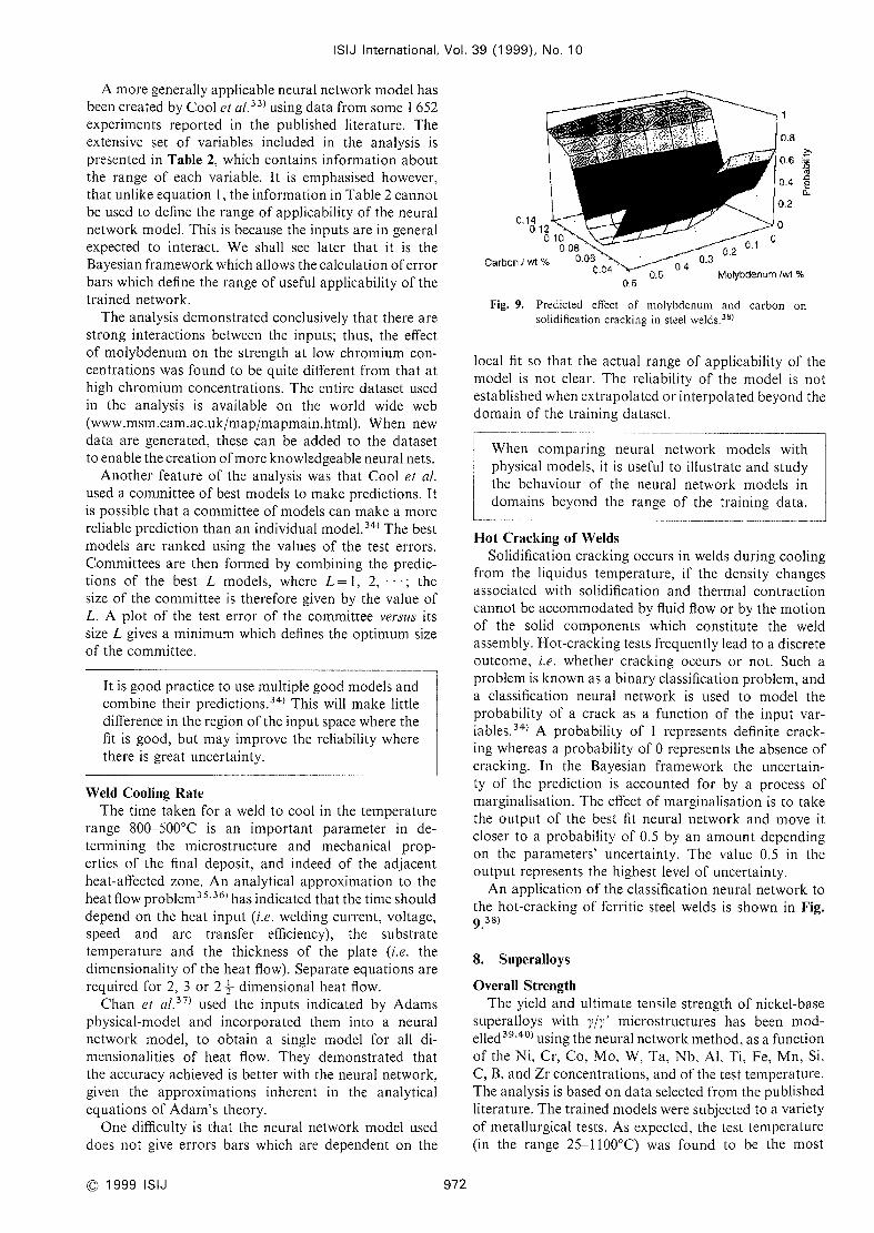
06Frg. 9. Predicted effect of molybdenumand carbon on

solidification cracking in steel welds.38)

972

10cal fit so that the actual range of applicability of the

model is not c]ear. The reliability of the model is notest',rblished whenextrapolated or interpo]ated beyondthe

domainof the training dataset,

Hot Cracking of WeldsSolidification cracking occurs in welds during coo]ing

from the liquidus temperature, if the density changesassociated with solidification and thermal contraction

cannot be accommodatedby fluid fiow or by the motionof the solid components which constitute the weldassembly. Hot-cracklng tests frequently lead to a discrete

outcome, i.e. whether cracking occurs or not. Such aproblem is knownas a binary classificatlon prob]em, anda classification neural network is used to model theprobability of a crack as a function of the input var-iables.34) A probability of I represents definite crack-ing whereas a probabi]ity of Orepresents the absence ofcracking. In the Bayesian framework the uncertain-ty of the prediction is accounted for by a process ofmarginalisatlon. The effect of marginalisation is to takethe output of the best fit neural network and moveit

closer to a probabi]ity of 0.5 by an amountdependingon the parameters' uncertainty. The value 0.5 in the

OLltpLlt represents the highest level of uncertainty.

Anapp]ication of the classification neural network tothe hot-cracking of ferritic steel welds is shownin Fig.9.38)

8. Superalloys

Overall StrengthThe yield and ultimate tensile strength of nickel-base

superalloys with yh,' microstructures has been mod-el]ed39•40) using the neural network method, as a functionof the Ni, Cr, Co. Mo, W, Ta, Nb, A], Ti, Fe, Mn, Si.

C, B, and Zr concentratlons, and of the test temperature.Theanalysis is basedon data selected from the publlshedliterature. The trained modelswere subjected to a variety

of metailurgical tests. As expected, the test temperature(in the range 25-1100'C) was found to be the most

ISIJ International, Vol.

slgnlficant variable Influencing the tensile properties,

both via the temperature dependenceof strengtheningmechanismsand due to variations in the y' fraction wlthtemperature. Since precipitation hardening is a dominantstrengthening mechanism, it was encouraglng that the

network recognised Ti, Al and Nb to be key factors

controlling the strength. Thephysical significance of theneural network was apparent in all the interrogationsperformed.

Oneexample illustrating this last point is presented in

Fig. 10. The softening of the y matrix is offset by the

remarkable reversible increase in the strength of the y'

with Increasing temperature.

A further revelation from the neura] network analysis

came from the error estimates, which demonstratedclearly that there are great uncertainties in the ex-perimental data on the effect of large concentrationsof molybdenumon the tensile properties. This hasidentified a region wherecareful experlments are needed;

molybdenumis knownto have a large influence on they/y' Iattice misfit.

9. Fatigue Properties

Fatigue is one of the most difficult mechanical prop-erties to predict. Anextensive literature review has beencarried out to assess methods for predicting the fatigue

crack growth rates.41) This Included an examinationof physical models, which where either found to lack

lOOOc$ :h

A*~: 800 ~\\

\+1~l' =~\~ /~ -- ~~~~ 600 \ ~~/\

/\ ~'~ ~~400C,~ \i15f

~ ~g 200 ~1;~ ' Experimental r8sults~

O 2 O 4 O 6 O 8O 10 O 12 OTemperature f 'C

Fig. lO. Predicted temperature dependence of the yield

strength of a y/y' superalloy (after Tancret),

~~

~-4,,

he)

\~-5~

hd/ ll-13 um~;

~-e 40-50 ,hm4;

r::,

~oo

-7

.r'lh-8

e B Io 404 iao~

39 (1999), No, 10

generallty or to give only qualitative indications of thetrends.41'42) Experiments on the initiation and prop-agation of cracks In turbine-disc superalloys have faiied

to clarify howfatigue theory could be used to makequan-titative predictions.

Aneural network methodhas therefore beenused after

identifying some51 variables that could be expected toinfluence the fatigue crack growth rate in nickel basesuperalloys.43) In fact, it is not difficult to compile aneven larger list of variables which could Influence fatigue

properties, but an over ambitlous choice of inputs is

likely to reduce the number of data available in theliterature.

~TlThe number of Inputs chosen is a compromise Ibetween the definition of the problem and theavailability of data. The neural network methodcannot copewith missing values. Anover ambltiouschoice of input variables will in genera] 1lmit the

number of complete sets of data available for

analysis. Onthe other hand, neglect of an importantvariable will lead to an increase in the noiseassociated with predictions.

Thevariables studied included the stress intenslty rangeAK, Iog{AK} chemical composition, temperature, grainsize, heat treatment, frequency, Ioad waveform, atmo-sphere. R-ratio, the dlstinction between short and longcrack growth, sample thickness and yleld strength. Theanalysls wasconducted on some1894data collected fromthe published literature. The reason for including both

AKand log{AK} as inputs is because the latter hasmetallurgical significance since a plot of the logarithmof the crack growth rate versus log{AK} is a simple andwell-established relationship. However, there mayexist

unknownand separate effects of AK, in which case that

should be included as an additional input. It is en-couraging that the trained network in fact assignedthe greatest significance to log{AK}.

Fig. Il.

If a certaln functional relationship Is expected be-

tween the raw output and a particular input, thanthat inpLrt can be included twice, in its functional

form and in its raw form. Theinclusion of the latter

prevents bias. _J

40

AK(MPam~) AK(MPam~)

Astroloy: (a) effect of grain size alone; (b) effect of heat treatment alone.43)

-3

~-4-Jo~)c,

\~-5~~;'~~ -e\ 11-13 uIns]

j1~t:'c-7

/+:

40-50 ,1 m~'

-B4 6 B iO

i~0 40

AK MPam~

973

40

@1999 ISIJ

ISIJ International, Vol. 39

The model, unlike any experimental approach, couldbe used to study the effect of each variable in isolation.

This gave interesting results. For example, it wasverified

that an increase in the grain size should lead to a decreasein the fatigue crack growth rate, whenthe grain size is

varied without affecting any other input. This cannot bedone in experiments because the change in grain size is

achieved by altering the heat treatment, which in turninfluences other features of the microstructure (Fig. 11).

It was also possible to confirm that log{AK} is morestrongly llnked to the fatigue crack growth rate than to

AK, as expected from the Paris law. There are manyother metallurgical trends revealed.43)

Theneural network modelcan in principle be usedto examine the effect of an individual input on the

output parameter, whereas this maybe incrediblydifficult to do experimentally.

In another approach44) a different neural computingapproach was used to focus on stage 11 of the Parisregime, where the growth rate should dependmainly onthe stress intensity range. Young's modulus and yield

strength. The model was used successfully in estimating

newtest data. The effect of the ultimate tensile strength

and phase stability was a]so investigated; although this

proved promlsing, it is probable that the results will be

moreconvincing whena greater range of data becomeavailable.

Fatigue ThresholdIn a recent study of the fatigue thresholds in nickel-base

superalloys, Schooling et al. have attempted to comparea "neurofuzzy" modelling approach with the classical

neural network.7) The application of fuzzy rules to the

network involves the biassing of the inputs according to

humanexperience.It was suggested that the fuzzy method has an ad-

vantage with restricted datasets because the complexityof the relationships can be restricted by the operator.This conclusion is surprising because the complexity of

a classical neural network, whenassessed for generalisa-tion, naturally tends to beminimised for small datasets.

Schooling et al. found it necessary to makesignificant

adjustments to the fuzzy rules in order reduce the meansquare error to a value comparable to the classical

network. It is evident that there is considerable operatorbias introduced in designing fuzzy networks. This maynot be satisfactory for complexproblemswherethe actualrelatlonships are not understood to begin with.

The comparison of the two methodsby Schooling etal. does not seemjustified because the predictions of theneurofuzzy methodwere not accompaniedby error bars(other than the meansquare error).

Creep of SuperalloysThe creep rupture life of nicke] base superalloys has

been modelled as a function of 42 variables includingCr, Co, C, Si. Mn, P, S, Mo, Cu, Ti, A1, B, N, Nb, Ta,Zr, Fe, W, V, Hf, Re, Mg, La and Th02'45) Othervariables include four heat treatment steps (characterisedby temperature, duration and cooling rate), the sample

(1 999). No. IO

@1999 ISIJ 974

shape and the solidification method.Sathyanarayanan et al.46) have developed a neural

network model for the "creep feed grinding" of nickel-'base superalloys and titanium alloys, using the feedrate, depth of cut and wheel bond type as Inputs, andthe surface finish, force and power as outputs.

Lattice Parameters of SuperalloysThe lattice constants of the yand y' phases of nickel

superalloys have been modelled using a neural networkwithin a Bayesian framework.47) Theanalysis wasbased

on newX-ray measurementsand peak separation tech-

niques, for a numberof alloys and as a function of tem-perature. These data were supplemented using the pub-lished literature.

Thelattice parameters of the two phaseswereexpressed

as a non-1inear functlon of eighteen variables includingthe chemical composition and temperature. It waspos-sible to estimate the uncertainties and the methodhasproved to be extremely useful in understanding boththe effect of solutes on the lattice mismatch, and onhowthis mismatchchanges with temperature.

10. Transformations

Martensite-start TemperatureMartensite forms without diffusion and has a well-

defined start-temperature (Ms), which for the majorityof engineering steels is only sensitive to the chemicalcomposltion of the austenite. There are numerous re-gression equations in the published literature, whichhave been used for manydccades in the estimation ofMs, mostly as a linear function of the chemical com-position. Vermeulen et a/.48) demonstrated that a neu-ral network model can do this muchmore effectively,

and at the same time demonstrated clear interactions

between the elernents. For example, the magnitude ofthe effect of a given carbon content on Ms is muchlarger at low manganeselevels than at high manganeseconcentrations. This is in contrast to all publishedequations where the sensitivity to carbon is independentof the presence of other alloying elements.

Continuous Cooling Transformation DiagramsThe transformation of austenite as the temperature

decreases during continuous cooling has been modelledwith the neural network method using the chemicalcomposition, the austenitisation temperature andcoolingrate as inputs.49] The results were concluded to besatisfactory but with large errors particularly for thebainite reaction. Theselarge errors were attributed partly

to noise in the experimental data, to the neglect ofaustenite grain size as an input, and to the assumptionthat all transformations occur at all cooling rates,

whereas this Is not the case in practice.

Thenetwork is empirical and hence permits a calcula-

tion of each transformation under all circumstances, evenwhenthis involves extrapolation into forbidden domains.This difficulty might be avoided by modelling the total

fraction of transformation and the transformation-start

temperatures separately, and then using a logical ruie to

determine whether the transformatlon is real or not.

ISIJ lnternational, Vol. 39 (1 999), No. 10

A further effect is illustrated by a later studyso); the

neural network calculations of CCTcurves as illustrated

in Fig. 12 appearjagged, rather than the expected smoothcurves. This Is because the points on the curve arecalculated individually and have been joined withoutaccounting for errors. If smooth curves are definitely

required, then the experimental curves should be rep-resented mathematically, and the parameters required

to describe these curves can be used as inputs. There will,

of course, be error bars to be taken into account butthese will be smoothly disposed about the mostexpected

curve.

T [~:)

900

800

700

eoe

~eo

400

~oo

200

1oo

+y

B

Mt

0.17 9~ C0-35 9e Ce,5a 9~ C

Fig. 12.

0,1 1 10 Ioo iC(lO 10000 100000t f$}

Theeffect of carbon on the CCTdiagram of an ailoy

steel as a function of the carbon concentration.so)

Austenite FormationMost commercial processes rely to someextent on

heat treatments which cause the steel to revert into theaustenitic condition. Thls includes the processes in-

volved in the manufacture of wrought steels, and in thefabrlcation of steel componentsby welding.

The formation of austenite during heating differs in

manywaysfrom those transformations that occur duringthe cooling of austenite. Both the diffusion coefficient

and the driving force increase with the extent of superheatabove the equilibrium temperature, so that the rate ofaustenite formation must increase indefinitely with

temperature.There is another important difference between the

transformation of austenite, and the transformation toaustenite. In the former case, the kinetics of transforma-tion can be described completely in terms of the alloy

composition and the austenite grain size. By contrast,the microstructure from which austenite maygrow canbe infinitely varied. Manymorevariables are therefore

needed to describe the kinetics of austenite formation.Gavardet al,sl) have created a neural network model

in which the Acl and Ac3 temperatures of steel areestimated as a function of the chemical composition andthe heating rate. Themodelhas beenvery revealing; someof the features are illustrated in Fig. 13. As might beexpected, the Acl temperature decreases with carbonconcentration reaching a limiting value which is veryclose to the eutectoid temperature of about 723'C. Thislatter limit is expected because of the slow heating rate

fhCJe*_.

U,~:

700oo 02 04 06 08 Io

c (Wt. %)

.~ve*_,

cr)

u.~

Fig. 13.

oo a2

u

~

7so

940

04 05 oS Ic

c (Wt. %)

820O1 1 1 10 100 1000 O1 1 1 10 100 Iaao

Heating Rate ('C/s) Heating Rate ('C/s)

(a, b) The predicted variation in the Acl and Ac3 temperatures of plain carbon steels as a function ofthe carbon concentration at a heating rate of l'Cs~1. (c,d) The predicted variation in the Acl and Ac3temperatures of an Fe-0.2 wto/o alloy as a function of the heating rate. In all of these diagrams, the lines

represent the ~l(T error bars about the calculated points. All the results presented here are based onmodels with four and two hidden units for the Acl and Ac3 temperatures respectively.

975 C 1999 ISIJ

ISIJ International. Vol, 39

and the fact that the test steel does not contain anysubstitutional solutes. Note that there is a slight un-derprediction of the Acl temperature for pure iron,

although the expected temperature of about 910'C is

within the 95 o/o confidence limits of the prediction (twicethe width of the error limits illustrated in Fig. 13).

By contrast, the Ac3 temperature appears to gothrough a minimumat about the eutectoid carbonconcentratlon. This is also expected because the Ae3temperature also goes through a minimum at theeutectoid composi~ion. Furthermore, uniike the Acltemperature, the minimumvalue of the calculated Ac3never reaches the eutectoid temperature; even at the slowheating rate it is expected that the austenite transforma-tion finishes at some superheat above the eutectoidtemperature, the superheat belng reasonabiy predictedto be about 25'C.

At slow heating rates, the predicted Acl and Ac3temperatures are in fact very close to the equilibriumAel and Ae3 temperatures and insensitive to the rate ofheating. As expected, they both increase more rapidlywhenthe heating rate rises exceeds about lO'C s~ l. Thesignificant maximumas a function of the heating rate is

unexpected and is a prediction which suggests that furtherexperiments are necessary.

Neural network analysis of published data canhelp identify experiments in two ways. First, un-expected trends mlght emerge. Secondly, the errorbars maybe so large as to makethe prediction un-certain, in which case experiments are necessary.

11. Steel Processing and Mechanical Properties

Hot Rolling

The properties of steel are great]y enhanced by therolling process. It is possible to cast steel into virtuallythe final shape but such a product will not have thequality or excellence of a carefully rolled product.

Singh et al.52) have deve]oped a neural network modelin which the yleld and tensile strength of the steel is

estimated as a function of some 108 variables, includ-ing the chemical composition and an array of rolling

parameters. Implicit in the rolling parameters is thethermal history and mechanical reduction of the slab asit progresses to the final product. The training data comefrom sensors on the rolling mill. There is therefore noshortage of data, the limitation in thls case being theneed to economise on computations. There are someexciting results which makesense from a metallurgicalpoint of view, together with somenovel predictions ona way to control the yield to tensile strength ratio. Asimilar mode] by Korczak et al.53) uses microstructuralparameters as inputs and has been applied to thecalculation of the ferrite grain size and property dis-

tribution through the thickness of the final plate.

Vermeulen et a/.54) have slmilarly modelled the

temperature of the steel at the last finishing stand. Theydemonstrated that it is definitely necessary to use anon-llnear representation of the input variables to obtainan accurate prediction of the temperature. The control

(1999), No. 10

C 1999 ISIJ 976

of strip ternperature on a hot strip mill rLlnoLlt table hasalso been modelled by Loney et a/.ss)

Heat TreatmentAJominy test is used to measurethe hardenability of

steel during heat treatment. Vermeulenet al. 56) havebeenable to accurately represent the Jominy hardness profilesof steels as a function of the chemica] composition andaustenitising temperature.

Mechanica] PropertiesThere are manyother examples of the use of neural

networks to describe the mechanical properties of steels;

Dumortier et al. have modelled the properties of micro-al]oyed stee]s57); Mllykoski58,59) has addressed theproblem of strength variations in thin steel sheets; mi-crostructureproperty relationshlps of C-Mnsteels60).

the tenslle properties of mechanically alloyed lron61,62)

with a comparlson with predictions using physicalmodels; the hot-torsion properties of austenite.63)

12. Polymeric and Inorganic Compounds

Neural network methodshave been used to model theglass transition temperatures of amorphousand semi-crystalline po]ymers to an accuracy of about 10K,and similar models have been developed for relaxatlontemperatures, degradation temperature, refractive index,tensile strength, e]ongation, notch strength, hardness,etc.6466) The molecular structure of the monomerlcrepeating unit Is described using topological indices fromgraph theory. The techniques have been exploited, forexample, in the design of polycarbonates for increasedimpact resistance. In another analysis, the glass transltion

temperature of linear homopolymershas beenexpressedas a function of the monomerstructure, and the modelhas been shown to generalise to unseen data to anaccuracy of about 35 K.67)

Comparisonwith QuantumMechanical CalculationsThere is an interesting study68) which claims that

neural networks are able to predict the equilibriumbond length, bond dissociation energy and equilibriumstretching frequency more accurately, and far morerapidly than quantummechanical calculations. Theworkdealt with diatomic molecules such as LiBr, using thirteeninputs: atomic number, atomic weight (to include isotopeeffects), valence electron configuration (s, p, d, .f elec-

trons) for both atoms, and the overall charge. Thecorresponding quantum mechanical calculations usedeffective core potentials as inputs. It was found that all

three molecular properties could be predicted moreaccurately using neural networks, with a considerablereduction in the computational effort.

Suchacomparison of a physica] modelwith one vjhichis empirical is not always likely to be fair. In general,

an appropriate neural network model should performbadly whencomparedwith a physical model, whenbothare presented with precisely identical data. This is becausethe neural network can only learn from the data it is

exposed to. By contrast, the physical model wlll contalnrelationships which have somejustification In science,

and which impose constraints on the behaviour of the

ISIJ International, Vol.

modelduring extrapolation. Asaconsequence, the neuralnetwork is likely to violate physical princip]es whenusedwithout restriction. Thecontinuous cooling transforma-tion curve model discussed above49'50) Is an examplewhere the neural network produces information in

forbidden domainsand produces jagged curves, which aphysical model using the samedata would not becausethe form of the curves would be based on phasetransformation theory [e,g. Ref. 69)].

13. Ceramics

Ceramic Matrix CompositesCeramic matrix composites rely on a weak interface

between the matrlx and fibre. This introduces slip anddebonding durlng deformation, thus avoidlng the catas-trophic propagation of failure. The mathernatlcal treat-

mentof the deformation has a large numberof variables

with manyfitting parameters. For an Al203 matrix SiCwhisker composite a constitutive law has been derivedusing an artificial neural network, using inputs generatedby finite element analysis.70)

Hybrid models can be created by training neuralnetworks on data generated by physical models.

Machining and ProcessingThere are manyexampleswhereneural networks have

been used to estimate machine-tool wear. For example,Ezuguwuet al.71) have modelled the tool 1lfe of amixed-oxide ceramlc cutting tool as a function of the

feed rate, cutting speed and depth of cut. Tribologyissues in machining, Including the use of neural networks,have been reviewed by Jahanmir.72)

Neural networks are also used routinely in the controlof cast ceramic products madeusing the slip castingtechnique, using variables such as the ambient conditions,

raw materlal information andproduction line settings.73)

In another application, scanning electron microscopeimages of ceramic powderswere digitised and processed

to obtain the particle boundary profile; this informa-tlon was then classified using a neural approach, withexceptionally good results even on unseen data.74)

14. Thin Films and Superconductors

A Iot of the materials science type issues about thin

films naturally involve deposition and characterisation.

The deposition process can be very compllcated to con-trol and is ideally suited for neural network applica-

tions.

Neural networks have been used to interpret Ramanspectroscopy data to deduce the superconductingtransition temperature of YBCOthin fiims during the

deposition process75); to characterise reflection hlgh-

energy electron dlffractlon patterns from semiconductorthin films in order to monitor the deposition process76).

to rapidly estimate the optical constants of thin films

using the computationa] results of a physical model ofthin films77). and there are numerous other simi]ar

examples.

977

39 (1999), No. 10

There is one particular application which falls in the

category of "alloy design"; Asada et a/.78) trained aneural network on a database of (Y1_*Ca*)Ba2Cu30_.and Y(Ba2_*Ca*)Cu30=,where -' is generally less than7, the ideal numberof oxygen atoms. The output pa-rameter was the superconducting transition tempera-ture as a function of x and z. They were thus able topredict the transition temperature of YBa2Cu30=dopedwith calclum. It was demonstrated that the highest

temperature is expected for x=0.3 and z=6.5 in

(Y1_*Ca*)Ba2Cu30=whereas a different behaviour oc-curs for Y(Ba2_*Ca*)Cu30..

l 5. Composites

There are manyapplications wherevibration informa-tlon can be used to assess the damagein compositestructures e.g.79 ~ 81) Acoustic emission signals have beenused to train a neural network to determine the burst

pressure of fiberglass epoxypr~ssure vessels.82) There has

even been an application trr the detection of cracks ineggs.83)

Onedifferent application is in the optimisation of thecuring process for polymer-matrix composites madeusing thermosetting resins.84) An interesting applica-tion is the modelling of damageevolution during forgingof AlSiC particle relnforced brake dlscs.85) Theauthors

were able to predict damagein a brake componentpreviously unseen by the neural network model.

Hwanget cd.86) compareda prediction of the failure

strength of carbon fibre reinforced polymer composite,madeusing a neural network model, against the Tsai-Wutheory and an alternative hybrid model. Of the threemodels, the neural network gave the smallest root-meansquare error. Nevertheless, the earlier commentsaboutthe validity of the neural network in extrapolation etc.

remain as a cautionary note in comparisons of neuraland physical models.

16. Publication

Theapplication of neural networks in materials scienceis a rapidly growing field. There are numerouspapersbeing published but the vast majority are of little useother than to the authors. This is becausethe publicationsalmost never include detailed algorithms, weights anddatabases of the kind necessary to reproduce the work.Work which cannot be reproduced or checked goesagainst the principles of scientlfic publication.

The mlnimuminformation required to reproduce atrained network is the structure of the network, the natureof the transfer functions, the weights corresponding to

the optimised network and the range of each input andoutput variable. Suchdetalled numerical information is

unlikely to be accepted for publication in journals. Thereis nowa world wide website where this information canbe logged for commonaccess:

wT'vvv.msm.ca,11.ac.uk/map/mcrpmain.html

It is also good practice to deposit the datasets used in

the development of neural networks in this materials

algorithms library.87)

@1999 ISIJ

ISIJ International. Vol. 39 (1999), No, 10

17. Summary

Neural networks are clearly extremely useful in recog-nising patterns in complex data. The resulting quantita-tive models are transparent; they can be interrogatedto reveal the patterns and the model parameters canbe studied to illuminate the significance of particularvariables. A trained network embodies the knowledgewithin the training dataset, and can be adapted asknowledge is accumulated.

Neural network analysis has had a liberating effect onmaterials science, by enabling the study of incrediblydiverse phenomenawhich are not as yet accessible tophysical modelllng. Themethodology is used extensivelyin process control, process design and alloy design. It is

a technique which should nowform a standard part ofthe undergraduate curriculum.

Acknowledgments

I amimmensely grateful to David MacKayfor his

help and friendship over manyyears, and to FranckTancret for reviewing the draft manuscript. I would alsolike to thank Dr Kaneaki Tsuzaki and the editorial boardof ISIJ International for inviting us to assemblea specialissue on neural networks.

l)

2)

3)

4)

5)

6)

7)

8)

9)

1O)

11)

12)

13)

l4)

15)

16)

17)

I8)

19)

20)

21)

2,~)

,~3)

24)

25)

26)

27)

28)

REFERENCESJ. S, Bowles and J. K. MacKenzie: Acta Metall., 2(1954), 129.

M. S. Wechsler, D. S. Lieberman and T. A. Read: Trans, Amer.Inst. Min. Meta!l. Engrs., 197 (1953), 1503.

W. Stevens and A. J. Haynes: J. Iron S!ee! h7st., 183 (1956), 349.

H. K. D. H. Bhadeshia: Acta Metall., 29 (1981), 1117.

D. J. C. MacKay:Neu"a! Conlputation, 4(1992), 415.

D. J. C. MacKay:Neu"a! C0'1rpu!crtion. 4(1992), 448.J. M. Schooling. M. Brownand P. A. S. Reed: Mafer. Sci. Eng.A. A260(1999), 222.S. H, ~iam and S. V. Oh: A!'p!ied 1,Itel!igence, 10 (1999), 53.

D. C. Lim and D. G. Gweon:J. Eng Ma'7uf:, 213 (1999), 51.

T. K. Mengand C. Butler: 1,It. J. Ac!v. Manuf. Techno!.. 13 (1997),

666,

W. Yi and I. S. Yun: KSME1,7/. J., 12 (1998), I150.

R. Polikar. L. Udpa, S. S. Udpaand T. Taylor: IEEET,'ans. 0,1

U!trasonics, Ferroe!ectrics andFrecf uenc;,' C0,It,'o!. 45(1998). 614.

T. W.Liao and K. Tang: Appliec[A,'!~ficia! Inte!!igence, 11 (1997),

l97.

A. Masnataand M. Sunseri: NDT&EInt., 29 (1996), 87.

D. Farson and J. Kern: Lase,'s in Enginee"i,1g, 4 (1995), 13.

L. M. Brownand R. Denale: Nav. Eng. J., 107 (1995), 179.

A. McNaband l. Dunlop: Insight, 37 (1995), Il.

E. V. Hill. P. L, Israel and G. L. Knotts: Mater. Eval., 51 (1993),

l040.

C. G. Winsdor, F. Anselme. L. Capineri and J. P. Mason: Br.J. Non-Desn'. Test., 35 (1993), 15.

J. D. Brown, M. G. Rodd and N. T. Williams: IronmakingSteelmaki,1g, 25 (1998), 199.

S. C. Juang, Y, S. TarngandH. R. Lii: J. Mate". P,'ocess. Tech,10!.,

75 (1998), 54.

P. Li. M. T. C. Fangand J. Lucas: J. Mate". P,'ocess. Tc'cll'70!.,

71 (1997). 288.

Y. M. Zhang, L. L1 and R. Kovacevic: J. Manuf: Sci. Eng.-Tra,',sactions of' ASME,119 (1997), 631.

H. S. Moonand S. J. Na: J. ManLtf, Sys!., 15 (1996), 392.

R. Kovacevic, Y. M. Zhangand L. Li: Weld. J., 75 (1 996). S317.

D Farson. K. Hillsley, J. Samesand R. Young: J. LaserApplicafions. 8(1996), 33.

Y. M. Zhang. R. Kovacevic and L. Li: 1,1!. J. Mach. Too!s Manuf.,36 (1996), 799.J. F. Knott: Fundamentals of Fracture Mechanics. Butter-

29)

30)

31)

32)

33)

34)

35)

36)

37)

38)

39)

40)

41)

42)

43)

44)

45)

46)

47)

48)

49)

50)

51)

52)

53)

54)

55)

56)

57)

58)

59)

60)

61)

62)

63)

worths, London, (1973).

A. H. Cottrell: Int. J. Pressu,'e Vessels Piping, 64 (1995), 171.H. K. D. H. Bhadeshia, D. J. C. MacKayand L.-E. Svensson:Ma!er. Sci. Tc'chnol., Il (1995), 1046,

B. Chan.M. Bibby andN. Holtz: Ca,1. Metall. Q., 34(1995), 353.L.-E. Svensson: Control of Microstructure and Properties in Steel

Arc Welds, CRCPress, London, (1994).

T. Cool. H. K. D. H. Bhadeshia and D. J. C. MacKay:Mater.Sci. E,7g. A, 223 (1997), 179.

D. J. C. MacKay:Mathematical Modelling of WeldPhenomenaIII, ed. by H, Cerjak and H. K, D. H. Bhadeshia, The Instituteof Materials, London, (1997), 359.C. M. Adams,Jr.: Weld. J., 37 (1958). S210.P. Jhaveri, W. G. Moffat and C. M. Adams,Jr.: We!d. J., 42(1962), 12.

B. Chan. M. Bibby and N. Holtz: Trans. Can. Soc. Mech. Eng.(CSME),20 (1996), 75.

K. Ichikawa, H. K. D. H. Bhadeshia and D. J. C. MacKay:Sci.

Tecllnol. Wc'Id. Joining, I (1996), 43.J. Jones and D, J. C. MacKay:8th Int. Symp. on Superalloys,ed, by R. D. Kissinger et al., TMS,Warrendale, (1996), 417.J. Jones, D. J. C. MacKayand H. K. D. H. Bhadeshia: Proc.4th Int. Symp,on AdvancedMaterials, eds. by Anwarul Haqetal., A, Q. KahnResearch Laboratories, Pakistan, (1995), 659.J. M. Schooling: The modelling of fatigue in nickel base alloys,

Ph,D. Thesis. University of Cambridge, (1997).J. M. Schooling and P. A. S. Reed: 8th Int. Symp.on Superalloys,ed. by R. D. Kissinger et a!.. TMS.Warrendale, (1996), 409.H. Fujii. D, J. C. MacKayand H. K. D. H. Bhadeshia: ISIJ 1,It.,

36 (1996), 1373.J. M. Schooling and P. A. S. Reed: Proc. 4th Int. Symp. onAdvancedMaterials, Ed. by Anwarul Haqet a!.. A. Q. KahnResearch Laboratories, Pakistan, (i995), 555.

H. Fujii. D. J. C. MacKay,H. K. D. H. Bhadeshia, H. Haradaand K. Nogi: 6th Leige Conference, Materials for AdvancedPowerEngineering, Univ. of Leige, (1998), 1401.

G. Sathyanarayanan, I. J. Lin and M, K. Chen: Int. J. ProductionResearch, 30 (1992), 2421.

S. Yoshitake, V. Narayan, H. Harada, H. K, D. H. Bhadeshiaand D. J. C. MacKay:ISIJ Int., 38 (1998), 495.

W. G. Vermeulen, P. F. Morris, A. P. de Weijer and S, van derZwaag: !,'0,1,naking Stee!making, 23 (1996), 433.

W, G. Vermeulen, S, van der Zwaag, P. F. Morris and T. deWeijer: Stee/ Res., 68 (1997), 72.

P. J. van der Wolk. C. Dorrepaal. J. Sietsma and S, van derZwaag: Intelligent Processing of High Performance Materials,Research and Technology Organization, Neuilly-sur-seine,

France, (1998), 6-1 to 6-6,

L. Gavard, H. K. D. H Bhadeshia, D. J. C. MacKayand S,

Suzuki: Mate,', Sci. Technol., 12 (1996), 453.S. B. Singh, H. K. D. H. Bhadeshia, D, J. C. MacKay.H. Careyand I. Martin: I,'on,naking Steelmalcing, 25 (1998), 355.P. Korczak, H. Dyja and E. Labuda: J. Mater. Process. Techno!.,80-1 (1998), 481.

W. G. Vermeulen, A. Bodin and S, van der Zwaag: Stee/ Res.,

68 (1997), 20.

D. Loney, I. Roberts and J. Watson: Ironmaking Steelmaking, 24(1997), 34.

W. G. Vermeulen. P. J, van der Wolk. A. P. de Weijer and S.

van der Zwaag: J. Mate,'. Eng. Pe,formance, 5(1996), 57.

C. Dumortier, P. Lehert. P. Krupa and A. Charlier: Mater. Sci.

Forum, 284 (1998), 393.

P, Myllykoski: J. Mate,'. Process. Tecll,10!., 79 (1998), 9.

P. Myllykoski. J. Larkiola and J. Nylander: J. Mate,'. P,'ocess,

Techno!., 60 (1996), 399.

Z. Y. Liu, W.D. Wangand W.Gao: J. Mater. P,'ocess. Tech,10l.,

57 (1996), 332.

A. Y. Badmos,H. K. D. H. Bhadeshla and D. J. C. MacKay:Mate,'. Sci. Tc'chnol., 14 (1998), 793.

A. Y. Badmosand H. K. D. H. Bhadeshia: Mater. Sci. Tecllno!.,

14 (1998), 1221.

V, Narayan. R. Abad-Lera, B. Lopez, H. K. D. H. Bhadeshiaand D. J. C. MacKay:ISIJ In!., 39 (1999). 999.

C1999 ISIJ 978

IS]J International, Vol. 39 (1999), No. 10

64) C. W. Ulmer. D. A. Smith, B. G. Sumpter and D. I. Noid:Comput. Theoretica/ Polym. Sci., 8(1998), 31 1.

65) B.G. SumpterandD.W.Noid:J. Therm.Anal.,46(1996), 833.

66) B, G. Sumpter and D. W. Noid: Mac,'omolecula,' Theory andSimulalions, 3(1994), 363.

67) S. J. Joyce. D. J. Osguthorpe, J. A. Padgett and G. J Price: J.

Chem.Soc.-Faraday Trans., 91 (1995), 2491.

68) T. R. Cundari and E. W, Moody:J. Cl7em. Inf. Comput, Sci., 37(1997), 871

.

69) H. K. D. H. Bhadeshia: MetalSci., 16 (1982), 159.

70) H. S. Rao, J. M. DeshpandeandA. Mukherjee: Sci. Eng. Compos.Mater., 6(1997), 225.

71) E. O. Ezugwu,S, J. Arthur and E. L Hines: J. Mater. Process.

Technol., 49 (1995), 225,

72) S. Jahanmir: Mac:hining Science and Technology, 2(1998), 137,

73) S. E. Martinez, A.E.Smith and B. Bidanda: J. Inte!ligentManuf.,

5(1994), 277.

74) G. Bonifazi and P. Burrascano: Adv. Polvde,' Technol., 5(1994),

225.

75) J. D. Busbee, B. Igelnik, D. Liptak. R, R. Biggers and I.

Maartense: Engineering Applications ofA,'t~cial Intelligence, Il

(1998), 637.

76) A. Bensaoula, H. A. Malki and A. M.Kwari: IEEETransactions

on Semiconducto,' Manufacturing, Il (1998), 421.

77)

78)

79)

80)

81)

82)

83)

84)

85)

86)

87)

Y. S. Ma. X. Liu, P. F. Guand J. F. Tang: App!ied Optics, 35(1996), 5035.

Y, Asada, E. Nakada, S. Matsumotoand H. Uesaka: Jout'nal ofSuperconductivity, 10 (1997), 23.

M. Q. Fengand F, Y. Bahng: J. Struct. Eng.ASCE,125 (1999),

265.

X. Xu. J. Evansand H. Vanderveldt: Modelling and Control ofJoining Processes, ed. by T. Zacharia. AmericanWelding Society,

Florida. USA,(1993), 203.

C. Doyle and G. Fernando: Smarl Mate,'ials a,Id St,'uctu,'es, 7(1998). 543.

M. E. Fisher and E. V. Hill: Mater. Eval., 56 (1998), 1395.

V. C Patel, R. W. McClendonand J. W. Goodrum:A,'t~ficicd

In!e!!igence App!icalions, 10 (1996), 19.

N. Rai and R, Pitchumani: J. Mater. P,'ocess. Manuf'. Sci., 6(1997), 39.

S. M. Roberts, J, Kusiak, Y.L. Liu, A. Forcellese and P. J.

Withers: J. Mater. Process. Technol., 80-1 (1998), 507.

W. Hwang.H. C. Park, K. S. Han: Mech. Compos.Mater., 34(1998), 28.

S. Cardie and H. K. D. H. Bhadeshia: Mathematical Mod-elling ofWeld Phenomena4, ed. by H. Cerjak and H. K. D. H.Bhadeshia, The Institute of Materials, London, (1998), 235.

979 C 1999 ISIJ