rev_frbrich2014q3.pdf
96
Economic Quarterly Volume 100,Number 3 Third Quarter 2014 Pages 183208 The Impact of the Durbin Amendment on Merchants: A Survey Study Zhu Wang, Scarlett Schwartz, and Neil Mitchell T he interchange fees associated with debit and credit cards have long been a controversial issue in the retail payments system. These fees are paid by a merchant to the cardholders bank (the so-called issuer) through the merchant-acquiring bank (the so-called acquirer) when credit or debit card payments are processed. Merchants have criticized that card networks (such as Visa and MasterCard) and their issuing banks have wielded market power to set excessively high interchange fees, which drive up merchants costs of accepting card payments. The controversy has also attracted great attention from policymakers, who are concerned that high interchange fees may inate retail prices and cause welfare losses to merchants and consumers. 1 To resolve this issue, a provision of the Dodd-Frank Act, known as the Durbin Amendment, mandates a regulation aimed at reducing debit card interchange fees and increasing competition in the payment processing industry. The Durbin Amendment directs the Federal Re- serve Board to regulate debit card interchange fees so that they are reasonable and proportional to the cost incurred by the issuer with We thank Dave Beck, Borys Grochulski, David Min, Ned Prescott, and Nicholas Trachter for helpful comments and Joseph Johnson for excellent research assistance. This study is based on a survey conducted by the Federal Reserve Bank of Rich- mond and Javelin Strategy & Research, a division of the Greenwich Group. The views expressed in this article are those of the authors and not necessarily those of the Federal Reserve Bank of Richmond or the Federal Reserve System. Correspon- dence: [email protected]. 1 In recent years, a sizable body of research literature has developed to evaluate whether fee setting in the payment card industry involves some market failure (see, for instance, Rochet and Tirole [2002, 2011], Wright [2003, 2012], Wang [2010], and Bedre-Defolie and Calvano [2013]). Wang (2012) provides a review of the interchange controversy in the U.S. market.
Transcript of rev_frbrich2014q3.pdf

Economic Quarterly� Volume 100, Number 3� Third Quarter 2014� Pages 183�208
The Impact of the DurbinAmendment on Merchants:A Survey Study
Zhu Wang, Scarlett Schwartz, and Neil Mitchell
The interchange fees associated with debit and credit cards havelong been a controversial issue in the retail payments system.These fees are paid by a merchant to the cardholder�s bank (the
so-called issuer) through the merchant-acquiring bank (the so-calledacquirer) when credit or debit card payments are processed. Merchantshave criticized that card networks (such as Visa and MasterCard) andtheir issuing banks have wielded market power to set excessively highinterchange fees, which drive up merchants� costs of accepting cardpayments. The controversy has also attracted great attention frompolicymakers, who are concerned that high interchange fees may in�ateretail prices and cause welfare losses to merchants and consumers.1
To resolve this issue, a provision of the Dodd-Frank Act, knownas the Durbin Amendment, mandates a regulation aimed at reducingdebit card interchange fees and increasing competition in the paymentprocessing industry. The Durbin Amendment directs the Federal Re-serve Board to regulate debit card interchange fees so that they are�reasonable and proportional to the cost incurred by the issuer with
We thank Dave Beck, Borys Grochulski, David Min, Ned Prescott, and NicholasTrachter for helpful comments and Joseph Johnson for excellent research assistance.This study is based on a survey conducted by the Federal Reserve Bank of Rich-mond and Javelin Strategy & Research, a division of the Greenwich Group. Theviews expressed in this article are those of the authors and not necessarily those ofthe Federal Reserve Bank of Richmond or the Federal Reserve System. Correspon-dence: [email protected].
1 In recent years, a sizable body of research literature has developed to evaluatewhether fee setting in the payment card industry involves some market failure (see,for instance, Rochet and Tirole [2002, 2011], Wright [2003, 2012], Wang [2010], andBedre-Defolie and Calvano [2013]). Wang (2012) provides a review of the interchangecontroversy in the U.S. market.
184 Federal Reserve Bank of Richmond Economic Quarterly
respect to the transaction.�The latter subsequently issued RegulationII (Debit Card Interchange Fees and Routing), which took e¤ect onOctober 1, 2011.
The regulation establishes a cap on the debit interchange fees that�nancial institutions with more than $10 billion in assets can chargeto merchants through merchant acquirers. The permissible fees wereset based on an evaluation of issuers�costs associated with debit cardprocessing, clearance, and settlement. The resulting interchange capis composed of the following: a base fee of 21 cents per transaction tocover the issuer�s processing costs, a 0.05 percent charge of the trans-action value to cover potential fraud losses, and an additional 1 centper transaction to cover fraud prevention costs if the issuer is eligible.This cap applies to both signature and PIN debit cards.
Since its implementation, the regulation has substantially reducedthe interchange revenues to covered issuers, while exempt small issuershave been well protected. The cap reduced the average debit inter-change fee by almost half from its pre-regulation level.2 As a result,covered issuers are losing billions of dollars every year in interchangerevenues (Wang 2012; Kay, Manuszak, and Vojtech 2014). However,due to lack of data, the regulation�s impact on merchants has not beenmuch examined, which motivated this study.
In this article, we report results from a merchant survey conductedby the Federal Reserve Bank of Richmond and Javelin Strategy & Re-search. The survey was performed two years after the regulation wasestablished. The results suggest that the regulation has had limited andunequal impact on merchants�debit acceptance costs. In the sample of420 merchants across 26 sectors, two-thirds reported no change or didnot know the change of debit costs post-regulation. One-fourth of themerchants, however, reported an increase of debit costs, especially forsmall-ticket transactions. Finally, less than 10 percent of merchants re-ported a decrease of debit costs. The impact varies substantially acrossdi¤erent merchant sectors.
The survey results also show asymmetric merchant reactions tochanging debit costs in terms of adjusting prices and debit restrictions.A sizable fraction of merchants are found to raise prices or debit re-strictions as their costs of accepting debit cards increase. However,few merchants are found to reduce prices or debit restrictions as debitcosts decrease. The sources of the asymmetric reactions remain a puz-zle, which may warrant additional research.
2 For an average debit card transaction at $40, the regulated interchange fee iscapped at 24 cents (21 cents + ($40 � 0.05%) + 1 cent).

Wang et al.: Impact of the Durbin Amendment on Merchants 185
The article is organized as follows. Section 1 provides industryand regulatory background, which motivates the study. Section 2 in-troduces the merchant survey and provides an overview of the data.Section 3 uses the survey results to analyze the impact of the regu-lation on merchants across di¤erent sectors in terms of debit costs,price change, and debit restrictions. Section 4 investigates merchants�asymmetric reactions to debit cost changes. Section 5 concludes.
1. MOTIVATION
To understand the debit interchange fee regulation, some familiaritywith the market is helpful. Debit cards are one of the most populargeneral-purpose payment cards in the United States. In 2012, theywere used in 47 billion transactions for a total value of $1.8 trillion.3
Debit card payments are authorized either by the cardholder�s signatureor by a PIN (personal identi�cation number). The former is calledsignature debit and the transactions are processed through either theVisa or MasterCard network. The latter is called PIN debit and thetransactions are processed through a dozen PIN debit networks.
Visa, MasterCard, and PIN debit networks are commonly referredto as four-party schemes because four parties are involved in each trans-action in addition to the network whose brand appears on the card.These parties include: (1) the cardholder who makes the purchase; (2)the merchant who makes the sale and accepts the card payment; (3)the �nancial institution that issues the card and makes the paymenton behalf of the cardholder (the so-called issuer); and (4) the �nancialinstitution that collects the payment on behalf of the merchant (theso-called acquirer).
In each of the debit card systems, interchange fees are collectivelyset by the network on behalf of their member issuers. When acceptinga debit card payment, a merchant needs to pay a fee, known as themerchant discount, to the acquirer. The acquirer then passes along afraction of that to the issuer as the interchange fee.
By regulating the interchange fee, the goal of the Durbin Amend-ment was to lower merchants�costs of accepting debit cards and to passalong the cost savings to consumers in terms of reduced retail prices. Afew years after the regulation was in place, however, it is unclear howe¤ectively the regulation has ful�lled its intention.
There are several important factors that may complicate the in-tended e¤ects on merchants. First, the regulation sets a cap on the
3 Source: The 2013 Federal Reserve Payments Study.
186 Federal Reserve Bank of Richmond Economic Quarterly
interchange fee but not on the merchant discount rate. The latter isthe ultimate fee that a merchant has to pay to the acquirer for accept-ing a card payment, which typically includes the interchange fee plusthe markup charged by the acquirer. Therefore, how much interchangereduction caused by the regulation can be passed along to merchantsmay depend on the pass-through rate of the acquirers.
Second, small issuers with less than $10 billion in assets are exemptfrom the regulation. According to the Federal Reserve Board Survey,exempt transactions constituted 36.5 percent of transaction value and37.3 percent of transaction volume across all networks in 2013, althoughthe proportions varied by network. For merchants whose customersprimarily use exempt debit cards, they may not necessarily see a fallof debit acceptance costs.
Third, the impact can vary substantially by merchant sector. Be-fore the regulation, card networks charged di¤erent interchange fees todi¤erent merchant sectors, and the fees varied in both level and struc-ture. For example, Visa debit cards charged $0.20+0.95% (with a $0.35cap) to supermarkets, $0.17+0.75% (with a $0.95 cap) to gas stations,$0.20 +0.95% to retail stores, $0.10+ 1.19% to restaurants, and $0.75to utility �rms.4 Therefore, how much a merchant can bene�t fromthe regulatory cap of $0.21+0.05% also depends on the sector-speci�cinterchange fees that the merchant used to pay prior to the regulation.
Fourth, interchange fees unintendedly rose for small-ticket trans-actions (Wang 2014). Prior to the regulation, most networks o¤ereddiscounted debit interchange fees for small-ticket transactions as a wayto encourage card acceptance by merchants for those transactions. Forexample, Visa and MasterCard used to set the small-ticket debit in-terchange rate at $0.04 plus 1.55 percent of the transaction value forsales of $15 and below. As a result, a debit card would only charge a7 cent interchange fee for a $2 sale or 11 cents for a $5 sale. However,in reaction to the regulation, card networks eliminated the small-ticketdiscounts and all transactions (except those on cards issued by exemptissuers) have to pay the maximum cap amount, $0.21+0.05%, set bythe regulation. Since merchants may have di¤erent compositions oftransaction sizes, they could be a¤ected di¤erently by the changes ofinterchange fees. However, merchants who specialize in small-tickettransactions would be most adversely a¤ected.
Finally, it is unclear how merchants would react to the regulation interms of changing prices and debit card restrictions. For merchants whohad a fall of debit costs, would they reduce prices and encourage the use
4 Source: Visa U.S.A. Interchange Reimbursement Fees, October 2010.

Wang et al.: Impact of the Durbin Amendment on Merchants 187
of debit cards? Alternatively, would merchants who had a rise of debitcosts do the opposite? To understand how much the regulation mayhave indirectly a¤ected consumers, we need to look at these importantissues.
In this article, we explore these issues using a merchant survey con-ducted two years after the regulation. Particularly, we investigate twosets of questions. First, we study how the regulation a¤ected mer-chants�costs of accepting debit cards and how the cost impact variedacross di¤erent merchant sectors for all transactions and for small-tickettransactions. Second, we study merchants�reactions to their debit costchanges through changing prices and through encouraging or restrictingdebit use. In terms of debit restrictions, we consider several practicesincluding minimum amount requirement, surcharge, and discount tonondebit payment means.
2. MERCHANT SURVEY
The Federal Reserve Bank of Richmond contracted with Javelin Strat-egy & Research, a division of the Greenwich Group, to create andlaunch an online and telephone survey, which was conducted in winter2013 through January 2014 to explore the merchant perspective of theDurbin Amendment�s impact.
Survey respondents were merchants serving on a pre-existing re-search panel who sell goods and services directly to consumers andaccept debit cards as a payment method.5 The sample comprises 420merchants across 26 sectors in all U.S. states with various attributes.
The survey also collects information regarding the regulation�s var-ious impacts on merchants: �rst, the costs of accepting debit cardsfor all transactions and for small-ticket transactions; second, the retailprices of goods or services; and third, the restrictions on debit carduse, including minimum amount, surcharge, and discount to nondebitpayment means.
Below we list a few sample survey questions. For simplicity, thesurvey uses the Durbin Amendment to refer to the original legislationand the resulting regulation.
� As you know, the Durbin Amendment was the recent policychange in 2011 which states that debit interchange fees be cappedat 21 cents per transaction. How have your debit card acceptancecosts changed after the Durbin Amendment came into e¤ect?
5 One limitation of the survey is that it does not include merchants who did notaccept debit cards at the time of the survey, so it does not provide information on howthe regulation may have a¤ected debit card acceptance.

188 Federal Reserve Bank of Richmond Economic Quarterly
(a) Costs increased; (b) No change in cost; (c) Costs decreased;(d) I do not know.
� After the Durbin Amendment in 2011, have you experienced animpact on the costs to accept debit card transactions with valuesof $10 and less? (a) Yes, the cost increased; (b) No, there hasbeen no impact; (c) Yes, the cost decreased; (d) I do not know.
� Has the Durbin Amendment directly impacted the price of thegoods or services you sell or o¤er? (a) Yes, prices were increasedbecause of Durbin; (b) No, Durbin had no impact on prices; (c)Yes, prices were decreased because of Durbin.
� Prior to the Durbin Amendment in 2011, did you set a minimumcharge to accept debit card payments? (a) Yes; (b) No; (c) Didnot accept debit cards prior to 2011.
Do you currently have a minimum charge to accept debit cardpayments? (a) Yes; (b) No.
Similarly, the survey also asked questions on surcharges and dis-counts on debit cards and other payment means, including cash, check,and credit cards, before and after the regulation.
To analyze the survey responses, we divide the data into two cat-egories. The �rst category comprises data on merchants� attributes,which will be used as explanatory variables in our following regressionanalysis. For each merchant, we have information on its sector, yearsin business, whether or not it accepts emerging payments (e.g., Square,Google, or PayPal), customer base, sales channels, geographic location,annual sales, and average ticket size.
The second category comprises data related to merchant impactfrom and reactions to the regulation, including cost changes for debitacceptance, price changes, and changing debit restrictions, which willserve as dependent variables in our regression analysis.
Table 1 provides a summary of the merchant attribute variables.Merchants in the sample belong to 26 sectors, of which fast food, restau-rants, and apparel each account for 11 percent�17 percent of the sample,and the other sectors each account for a share below 10 percent. Someof the merchants operate in multiple sectors, so the sum of sector sharesshown in Table 1 exceeds 100 percent. Of the merchants who reported,3.8 percent said they had existed in business less than two years; 24.5percent accepted emerging payments; and 46.7 percent were primarilyserving repeat customers. Also, 86.4 percent of the merchants wereselling through physical stores, 40.7 percent through online, and 35.2percent through other sales channels (e.g., catalog and mail orders).Moreover, merchants in the sample distribute quite evenly across nine

Wang et al.: Impact of the Durbin Amendment on Merchants 189
Table 1 Summary of Merchant Attribute Variables (N=420)
Merchant Sectors Other AttributesApparel 10.5% New Firm 3.8%Art 2.4% Emerging Payments 24.5%Auto 6.7% Repeat Customers 46.7%Casinos 1.7% Physical Store 86.4%Consumer Electronics 7.9% Online Channel 40.7%Convenience Stores 6.7% Other Channel 35.2%Delivery Services 2.9% East North Central 24.3%Department Stores 3.1% East South Central 13.8%Discount Retail 5.2% Middle Atlantic 23.8%Education 0.5% Mountain 17.4%Entertainment 8.3% New England 16.7%Fast Food 16.7% Paci�c 28.3%Grocery Stores 6.0% South Atlantic 28.1%Home Furnishings 6.0% West North Central 16.9%Home Improvement 5.5% West South Central 21.0%Hospitality 3.8% Sales < $100,000 18.1%Maintenance 4.0% Sales $100,000�$1M 30.7%Medical 6.9% Sales $1M�$10M 25.7%O¢ ce Products 2.9% Sales $10M�$100M 16.4%Other Sector 3.3% Sales > $100M 3.8%Real Estate 1.4% Sales Missing 5.2%Restaurants 10.7% Average Ticket < $10 23.81%Services 5.0% Average Ticket $10�$50 22.14%Sporting Goods 3.8% Average Ticket $50�$250 30.71%Toys 3.8% Average Ticket >$250 23.33%Transportation 4.5%
census districts, annual sales ranges (except for the largest sales rangeabove $100 million), and average ticket sizes.
Table 2 provides a summary of merchant impact/reaction variables.Most respondents (67 percent) reported no change or did not know thechange in their overall costs of accepting debit cards post-regulation.Among those who did see a change in debit costs, about three times asmany (25 percent over 8 percent) reported a cost increase as those whoreported a cost decrease. A similar pattern is found for small-tickettransactions, while nine times as many (27 percent over 3 percent)respondents reported a cost increase as those who reported a cost de-crease.
The majority of respondents (75 percent) reported no price changedue to the regulation. For those who had a price change, 11 times more(23 percent over 2 percent) reported price hikes than cuts. Meanwhile,most respondents (76 percent) reported no increase or decrease in therestrictions on debit card use. For those who did report a change, theyare even on each side (12 percent and 12 percent).

190 Federal Reserve Bank of Richmond Economic Quarterly
Table 2 Summary of Merchant Impact/Reaction Variables(N=420)
Stay the Don�tMerchant Average Decrease Same Increase KnowCost Change 8% 41% 25% 26%Small-Ticket Cost Change 3% 47% 27% 24%Price Change 2% 75% 23% 0%Debit Restriction Change 12% 76% 12% 0%
MinimumAmount Surcharge Discount Others
Before Durbin 26% 24% 20% 55%After Durbin 29% 20% 20% 58%
Note that the restrictions on debit card use are measured by threepractices, namely, whether the merchant imposes a minimum amountrequirement on debit transactions, surcharges debit cards, or o¤ers dis-counts only to nondebit payment means. In the case that a merchantadded more (or dropped some) restrictions on accepting debit cards af-ter the regulation, we call it increasing debit restrictions (or decreasingdebit restrictions).6
Table 2 also provides information on merchants�practices on eachspeci�c debit restriction before and after the regulation. In the sam-ple, 26 percent of merchants imposed the minimum amount on debittransactions prior to the regulation, and the fraction changed to 29 per-cent post-regulation. Meanwhile, the fraction of merchants surchargingdebit cards changed from 24 percent to 20 percent, and the fraction ofmerchants o¤ering discounts only to nondebit payment means remainedat 20 percent.
Finally, Table 3 drops multisector merchants and summarizes mer-chant impact/reaction variables based on 362 merchants that only op-erate in one sector. For each variable, we report the average fractionacross 26 sectors so that the results would not be driven by certain sec-tors that have more observations. Nevertheless, the patterns are verysimilar to Table 2.
6 Here, a merchant�s change in debit restrictions is measured by comparing the num-bers of restrictions before and after the regulation. We use this measure for the analysisin Section 3. However, in Section 4, we take a step further to look at each type of thethree restrictions.

Wang et al.: Impact of the Durbin Amendment on Merchants 191
Table 3 Summary of Merchant Impact/Reaction VariablesBased on One-Sector Merchants (N=362)
Stay the Don�tSector Average Decrease Same Increase KnowCost Change 9% 43% 25% 23%Small-Ticket Cost Change 3% 49% 25% 23%Price Change 2% 76% 23% 0%Debit Restriction Change 13% 73% 14% 0%
3. REGULATORY IMPACT ON MERCHANTS
In this section, we conduct ordered logit regressions to estimate thedebit interchange regulation�s impact on merchants on several aspects,including the change of merchants�costs of accepting debit cards forall transactions and for small-ticket transactions, price changes, andthe change of debit restrictions. In this analysis, we do not intend toidentify any causal e¤ects or impact channels. Rather, our focus is toinvestigate how the regulation�s impact varies across di¤erent merchantsectors.
In each of the regressions, we include sector dummies together withother merchant attribute variables listed in Table 1.7 The sample weuse comprises merchants operating only in one sector, so that the es-timated sector dummies clearly identify the sector �xed e¤ect, and weexclude merchants who reported �do not know�regarding their debitcost changes wherever appropriate.
The ordered logit regression assumes the following structure. Sup-pose the underlying process to be characterized is
y� = x� + ";
where y� is the exact but unobserved dependent variable, x is a vectorof independent variables, and we observe the categories of outcome
y =
8<: 0 (decrease); if y� � u1;1 (unchanged); if u1 < y� < u2;2 (increase); if y� � u2;
7 Note that we exclude average ticket size as an explanatory variable in all regres-sions because of its duplication with the sector �xed e¤ect.

192 Federal Reserve Bank of Richmond Economic Quarterly
Table 4 Debit Cost Change for All Transactions (EstimatedProbabilities)
Merchant Sector Decrease Stay the Same IncreaseApparel 0.070 0.632*** 0.298Art 0.357 0.589** 0.054Auto 0.100* 0.677*** 0.224**Casinos 0.112** 0.686*** 0.202**Consumer Electronics 0.126** 0.693*** 0.181**Convenience Stores 0.242 0.667*** 0.091Delivery Services 0.000 0.000 1.000***Department Stores 0.032 0.474*** 0.495***Discount Retail 0.059 0.603*** 0.338*Entertainment 0.163* 0.696*** 0.141*Fast Food 0.016* 0.327*** 0.657***Grocery Stores 0.026* 0.433*** 0.541***Home Furnishings 0.259** 0.658*** 0.084*Home Improvement 0.034 0.489** 0.478*Hospitality 0.106 0.682*** 0.211Maintenance 0.166* 0.696*** 0.138Medical 0.141 0.696*** 0.162O¢ ce Products 0.024 0.414* 0.561**Other Sector 0.038 0.515*** 0.447**Real Estate 0.038 0.513*** 0.449**Restaurants 0.047** 0.561*** 0.392***Services 0.140** 0.696*** 0.164***Sporting Goods 0.259** 0.658*** 0.084*Toys 0.077 0.647*** 0.276Transportation 0.139*** 0.696*** 0.165***Sector Average 0.111 0.576 0.313
Notes: ***p<0.01, **p<0.05, *p<0.1. The estimated probabilities are based onan ordered logit regression that includes other regressors as shown in Table 1.(Obs: 254; R2: 0.17).
where u1 and u2 are latent thresholds. Then the ordered logit regressionwill use the observations on y, which are a form of censored data on y�
to estimate the parameter vector � and the thresholds u1 and u2.Tables 4 and 5 report the model-estimated distributions of debit
cost change for all transactions and for small-ticket transactions across26 merchant sectors, taking all the other merchant attribute variablesat their mean values.
The results suggest limited and unequal impact on merchant debitcosts: Averaging across 26 sectors, 11.1 percent of merchants are es-timated to have reduced debit costs for all transactions, 31.3 percenthave increased costs, and 57.6 percent are unchanged. For small-ticket

Wang et al.: Impact of the Durbin Amendment on Merchants 193
Table 5 Debit Cost Change for Small-Ticket Transactions(Estimated Probabilities)
Merchant Sector Decrease Stay the Same IncreaseApparel 0.008 0.577*** 0.415***Art 0.081 0.860*** 0.060Auto 0.071* 0.861*** 0.068*Casinos 0.000 0.000 1.000***Consumer Electronics 0.026 0.802*** 0.172Convenience Stores 0.058 0.859*** 0.083Delivery Services 0.003 0.371 0.626**Department Stores 0.038** 0.838*** 0.125***Discount Retail 0.006 0.501** 0.493**Entertainment 0.025 0.796*** 0.180**Fast Food 0.004 0.396*** 0.600***Grocery Stores 0.017 0.743*** 0.239*Home Furnishings 0.167** 0.806*** 0.027*Home Improvement 0.030 0.816*** 0.155Hospitality 0.018 0.745*** 0.238*Maintenance 0.003 0.316 0.681***Medical 0.018 0.751*** 0.231**O¢ ce Products 0.003 0.364 0.633Other Sector 0.013 0.696*** 0.290Real Estate 0.007 0.545** 0.448Restaurants 0.022* 0.782*** 0.195**Services 0.035** 0.831*** 0.134***Sporting Goods 0.016 0.732*** 0.252Toys 0.008 0.593*** 0.399**Transportation 0.020 0.764*** 0.216Sector Average 0.028 0.654 0.318
Notes: ***p<0.01, **p<0.05, *p<0.1. The estimated probabilities are based onan ordered logit regression that includes other regressors as shown in Table 1.(Obs: 259; R2: 0.20).
transactions, only 2.8 percent are estimated to have reduced debit costs,31.8 percent have increased costs, and 65.4 percent are unchanged.8
As mentioned before, the mixed cost impact on merchants mayresult from several complication factors discussed in Section 1, whichcould vary substantially by sector. Merchants who had reduced to-tal debit costs could be those who gained more from the large-tickettransactions than losing on small-ticket ones. Merchants who hadno change on total debit costs could be those whose customers wereprimarily using debit cards from exempt issuers or whose loss from
8 Our estimated distributions are fairly consistent with the pattern found in the rawdata. However, the regression analysis allows us to control other merchant attributeswhile identifying the sector e¤ects.
194 Federal Reserve Bank of Richmond Economic Quarterly
small-ticket transactions balanced out gains from large-ticket ones. Fi-nally, merchants who had increased total debit costs could be thosewho specialized on small-ticket transactions.
The estimated cost impact varies substantially across merchantsectors:
� Top sectors of total debit cost reduction are home furnishings(25.9 percent), sporting goods (25.9 percent), maintenance (16.6percent), entertainment (16.3 percent), and services (14.0percent).
� Top sectors of total debit cost increase are delivery services (100percent), fast food (65.7 percent), o¢ ce products (56.1 percent),grocery stores (54.1 percent), and home improvement (47.8percent).
� Top sectors of small-ticket debit cost increase are casinos (100percent), maintenance (68.1 percent), delivery services (62.6 per-cent), fast food (60.0 percent), and discount retail (49.3 percent).
It is intuitive that fast food and delivery services rank top in bothtotal debit cost increase and small-ticket debit cost increase. Presum-ably, merchants in those sectors deal with mostly small-ticket trans-actions, so they were likely to feel cost increases in both small-ticketand total debit transactions. However, home furnishings and sportinggoods rank top in total debit cost reduction, which may re�ect theirrelatively large transaction sizes.
Table 6 reports the model-estimated probabilities of price change.The results suggest the regulation has had a limited impact on prices.Averaging across all sectors, it is estimated that the majority of mer-chants (77.2 percent) did not change prices post-regulation, very fewmerchants (1.2 percent) reduced prices, while a sizable fraction of mer-chants (21.6 percent) increased prices.
The estimated price change pattern also varies by sector:
� Top sectors of price increase are delivery services (100 percent),o¢ ce products (77.8 percent), fast food (39.6 percent), and ap-parel (28.6 percent).
� Top sectors of price decrease are auto (5.6 percent), other sector(4.3 percent), sporting goods (2.7 percent), and art (2.5 percent).
Table 7 reports the model-estimated probabilities of changing debitrestrictions. Again, the results suggest limited and unequal impact.Averaging across all sectors, it is estimated that the majority of mer-chants (76.6 percent) did not change debit restrictions post-regulation,

Wang et al.: Impact of the Durbin Amendment on Merchants 195
Table 6 Change of Prices: Estimated Probabilities
Merchant Sector Decrease Stay the Same IncreaseApparel 0.002 0.711*** 0.286***Art 0.025** 0.940*** 0.035Auto 0.056** 0.929*** 0.015*Casinos 0.037 0.940*** 0.024Consumer Electronics 0.006 0.863*** 0.131Convenience Stores 0.002 0.686*** 0.312Delivery Services 0.000 0.000 1.000***Department Stores 0.002 0.655** 0.343Discount Retail 0.005 0.827*** 0.168Entertainment 0.009 0.895*** 0.097Fast Food 0.001 0.602*** 0.396***Grocery Stores 0.003 0.734*** 0.264*Home Furnishings 0.015 0.929*** 0.056Home Improvement 0.004 0.822*** 0.174Hospitality 0.006 0.866*** 0.127*Maintenance 0.002 0.661*** 0.337*Medical 0.006 0.852*** 0.142*O¢ ce Products 0.000 0.222 0.778***Other Sector 0.043** 0.937*** 0.020*Real Estate 0.009 0.902*** 0.089Restaurants 0.002 0.727*** 0.270***Services 0.011 0.910*** 0.080*Sporting Goods 0.027** 0.941*** 0.032**Toys 0.032 0.941*** 0.027Transportation 0.004 0.798*** 0.199Sector Average 0.012 0.772 0.216
Notes: ***p<0.01, **p<0.05, *p<0.1. The estimated probabilities are based onan ordered logit regression that includes other regressors as shown in Table 1.(Obs: 340; R2: 0.21).
12.4 percent of merchants increased debit restrictions, while 10.9 per-cent decreased restrictions.
The estimated changing debit restriction pattern varies by sector:
� Top sectors of increased debit restrictions are maintenance (30.8percent), other sector (25.7 percent), transportation (20.2 per-cent), and hospitality (18.9 percent).
� Top sectors of reduced debit restrictions are sporting goods (26.5percent), services (16.9 percent), fast food (11.8 percent), andhome improvement (11.8 percent).
It is interesting to see sporting goods ranks top in both price reduc-tion and debit restriction reduction. This is consistent with the �ndingabove that the sector ranks top in the total debit cost reduction. Incontrast, fast food ranks top in price increase but also in reducing

196 Federal Reserve Bank of Richmond Economic Quarterly
Table 7 Change of Debit Restrictions: EstimatedProbabilities
Merchant Sector Decrease Stay the Same IncreaseApparel 0.161** 0.792*** 0.047**Art 0.142 0.804*** 0.054Auto 0.112* 0.818*** 0.070*Casinos 0.092* 0.823*** 0.0860*Consumer Electronics 0.073 0.820*** 0.107Convenience Stores 0.099** 0.822*** 0.080**Delivery Services 0.011 0.517* 0.472Department Stores 0.033 0.750*** 0.217Discount Retail 0.255 0.718*** 0.027Entertainment 0.064* 0.814*** 0.122**Fast Food 0.118** 0.816*** 0.066**Grocery Stores 0.111** 0.818*** 0.071*Home Furnishings 0.042 0.780*** 0.178Home Improvement 0.118** 0.816*** 0.066**Hospitality 0.039 0.772*** 0.189*Maintenance 0.021 0.671*** 0.308**Medical 0.117* 0.816*** 0.067*O¢ ce Products 0.041 0.776*** 0.183Other Sector 0.027* 0.717*** 0.257**Real Estate 0.387 0.599** 0.015Restaurants 0.109*** 0.819*** 0.072***Services 0.169* 0.786*** 0.045Sporting Goods 0.265** 0.710*** 0.026Toys 0.092 0.822*** 0.085Transportation 0.036 0.762*** 0.202*Sector Average 0.109 0.766 0.124
Notes: ***p<0.01, **p<0.05, *p<0.1. The estimated probabilities are based onan ordered logit regression that includes other regressors as shown in Table 1.(Obs: 340; R2: 0.10).
debit restrictions. This may re�ect the nature of the business wheremerchants value particularly the checkout speed so they responded toa rise of debit costs mainly through a price increase instead of addingdebit restrictions.
4. MERCHANT REACTIONS TO DEBIT COSTCHANGES
In this section, we take a step further to investigate the impact channelsbehind the intended and unintended consequences of the regulation.We examine two sets of questions. One is on the intended e¤ects: Didlower debit costs lead to lower retail prices and debit restrictions? The

Wang et al.: Impact of the Durbin Amendment on Merchants 197
other is on the unintended e¤ects: Did higher debit costs lead to higherretail prices and debit restrictions?
The analysis is conducted using logit regressions, which connectsurvey respondents�answers of their post-regulation debit cost changeswith their reported changes of prices and debit restrictions. The samplewe use again comprises merchants operating only in one sector, butwe no longer need to exclude merchants who reported �do not know�regarding their debit cost changes.
Reactions to a Debit Cost Decrease
We �rst analyze merchants�reactions to a debit cost decrease. We run�ve separate logit regressions, with the binary dependent variables be-ing merchants�status post-regulation. Speci�cally, in each of the �veregressions, the dependent variable takes the value of 1 (otherwise, 0)if a merchant satis�es the respective criteria: (1) price decrease; (2) nodebit restriction; (3) no minimum amount requirement on debit trans-actions; (4) no surcharge on debit cards; and (5) no discount o¤eredonly to nondebit payment means.
On the explanatory variable side, we control for merchants�debitrestrictions prior to the regulation as well as other attributes listed inTable 1. We also divide merchants into four dummy groups accordingto their debit cost changes: (1) small-ticket costs decreased, total costsdecreased; (2) small-ticket costs decreased, total costs did not decrease;(3) small-ticket costs did not decrease, total costs decreased; (4) small-ticket costs did not decrease, total costs did not decrease. Using thesedummy variables will allow us to separate the variation of merchantreactions due to di¤erent types of cost shocks.
Table 8 reports the logit regression results. The �rst column is theprice reaction. However, the regression fails to run given that too fewmerchants reported a price reduction.
The next four columns in Table 8 show the estimated merchantreactions in terms of debit restrictions. First, the results suggest thatmerchants tend to have persistent policies. If a merchant did not im-pose any debit restrictions (or speci�cally, requiring minimum amounton debit transactions, surcharging debit cards, or o¤ering discount onlyto nondebit payment means) prior to the regulation, it is likely the mer-chant would not restrict debit post-regulation. The persistence e¤ectsare statistically and economically signi�cant. To put the estimationresults into perspective, Table 9 reports the estimated probabilities.Holding other explanatory variables at their mean values, if a merchantdid not impose any debit restrictions prior to the regulation, there

198Federal
Reserve
Bank
ofRichm
ondEconom
icQuarterly
Table 8 Logit Regressions: Merchant Reactions to a DebitCost Decrease
Not No No NoVariables Price Restricting Minimum Surcharge Discount
Decrease Debit After After After AfterNot Restricting Debit Before � 0.746***
(0.051)No Minimum Before � 0.611***
(0.072)No Surcharge Before � 0.877***
(0.048)No Discount Before � 0.889***
(0.058)Small-Ticket Costs Decreased, � 0.258*** 0.018Total Costs Decreased (0.047) (0.012)
Small-Ticket Costs Decreased, � �0.233 0.018 0.015Total Costs Did Not Decrease (0.409) (0.012) (0.019)
Small-Ticket Costs Did Not � �0.004 0.125** �0.027 �0.005Decrease, Total Costs Decreased (0.184) (0.058) (0.073) (0.018)
Other Regressors � Included Included Included IncludedObs 334 330 285 324Pseudo R2 � 0.530 0.383 0.663 0.659
Notes: Robust standard errors in parentheses. ***p<0.01, **p<0.05, *p<0.1.

Wangetal.:
Impact
oftheDurbinAmendmentonMerch
ants
199
Table 9 Merchant Reactions to a Debit Cost Decrease(Estimated Probabilities)
Not No No NoVariables Restricting Minimum Surcharge Discount
Debit After After After AfterHad Restriction/Minimum/Surcharge/ 0.193*** 0.305*** 0.120*** 0.105*Discount Before (0.044) (0.068) (0.047) (0.055)
Didn�t Have Restriction/Minimum/ 0.939*** 0.916*** 0.997*** 0.994***Surcharge/Discount Before (0.019) (0.022) (0.003) (0.004)
Small-Ticket Costs Decreased, 0.975*** 1.000***Total Costs Decreased (0.030) (0.000)
Small-Ticket Costs Decreased, 0.581 1.000*** 0.993***Total Costs Did Not Decrease (0.417) (0.000) (0.019)
Small-Ticket Costs Did Not 0.713*** 0.949*** 0.953*** 0.973***Decrease, Total Costs Decreased (0.183) (0.054) (0.080) (0.022)
Small-Ticket Costs Did Not Decrease, 0.717*** 0.824*** 0.982*** 0.978***Total Costs Did Not Decrease (0.042) (0.031) (0.013) (0.012)
Other Regressors At mean At mean At mean At meanObs 334 330 285 324
Notes: Standard errors in parentheses. ***p<0.01, **p<0.05, *p<0.1.

200 Federal Reserve Bank of Richmond Economic Quarterly
is a 93.9 percent chance that the merchant will not restrict debit usepost-regulation. Otherwise, the chance would be reduced to 19.3 per-cent. A similar pattern is found for each of the speci�c restrictions,namely minimum amount, surcharge, and discount.
Second, the reduction of debit costs does not seem to have a bigimpact on reducing debit restrictions. As shown in Table 8, the dummyvariable �small-ticket costs did not decrease, total costs decreased� isnot statistically signi�cant for most regressions except for that of min-imum amount. Table 9 reports the estimated probabilities. Holdingother explanatory variables at their mean values, if a merchant did nothave a reduction for either the total debit costs or the small-ticket costs,there is a 71.7 percent chance that the merchant would not impose anydebit restrictions post-regulation. In comparison, if the merchant be-longs to the group that �small-ticket costs did not decrease, total costsdecreased,�the chance of not restricting debit use is 71.3 percent post-regulation, almost no di¤erence. The same pattern is found for theregressions on surcharge and discount. However, there is some e¤ectin the minimum amount regression, though the magnitude is relativelysmall. As shown in Table 9, if a merchant did not have a reductionfor either the total debit costs or the small-ticket costs, there is an82.4 percent chance that the merchant would not impose a minimumamount on debit transactions post-regulation. In contrast, if the mer-chant belongs to the group that �small-ticket costs did not decrease,total costs decreased,�the chance of not imposing a minimum amounton debit transactions would rise to 94.9 percent post-regulation, a 12.5percent increase.
Note that most merchants in the sample who had a debit cost de-crease belong to the group �small-ticket costs did not decrease, totalcosts decreased.�As shown in Table 10, among the 362 one-sector mer-chants in the sample, they account for 7.1 percent. In contrast, only1.8 percent of merchants belong to the group �small-ticket costs de-creased, total costs decreased,� and 0.6 percent belong to the group�small-ticket costs decreased, total costs did not decrease.� Accord-ingly, the estimated parameters for the latter two group dummies areless meaningful. In fact, they are dropped from some of the regressionsdue to lack of variation.
Reactions to a Debit Cost Increase
We then analyze merchants�reactions to a debit cost increase. We alsorun �ve separate logit regressions, with each of the dependent variablesbeing a merchant�s status post the regulation: (1) price increase; (2)restricting debit use; (3) imposing minimum amount on debit

Wangetal.:
Impact
oftheDurbinAmendmentonMerch
ants
201
Table 10 Variation of Debit Cost Decrease Across MerchantSectors
Small-Ticket Costs Small-Ticket Costs Small-Ticket CostsSmall-Ticket Costs Decreased, Total Did Not Decrease, Did Not Decrease,Decreased, Total Costs Did Not Total Costs Total Costs Did
Merchant Sector Costs Decreased Decrease Decreased Not DecreaseApparel 0% 0% 17% 83%Art 13% 0% 13% 75%Auto 0% 0% 13% 88%Casinos 0% 0% 0% 100%Consumer Electronics 0% 0% 8% 92%Convenience Store 15% 0% 15% 69%Delivery Services 0% 0% 0% 100%Department Stores 0% 0% 0% 100%Discount Retail 8% 0% 0% 92%Entertainment 0% 0% 10% 90%Fast Food 0% 0% 2% 98%Grocery Stores 0% 6% 0% 94%Home Furnishings 0% 0% 0% 100%Home Improvement 0% 0% 10% 90%Hospitality 0% 0% 7% 93%Maintenance 0% 0% 17% 83%Medical 0% 0% 16% 84%O¢ ce Products 0% 17% 0% 83%Other Sector 8% 0% 0% 92%Real Estate 0% 0% 0% 100%Restaurants 3% 0% 0% 97%Services 0% 0% 10% 90%Sporting Goods 0% 0% 25% 75%Toys 0% 0% 17% 83%Transportation 0% 0% 0% 100%Merchant Average 1.8% 0.6% 7.1% 90.6%Sector Average 1.9% 0.9% 7.2% 90.1%

202 Federal Reserve Bank of Richmond Economic Quarterly
transactions; (4) surcharging debit cards; and (5) o¤ering discountsonly to nondebit payment means.
On the explanatory variable side, we again control for merchants�debit restrictions prior to the regulation, debit cost changespost-regulation, and other merchant attributes.
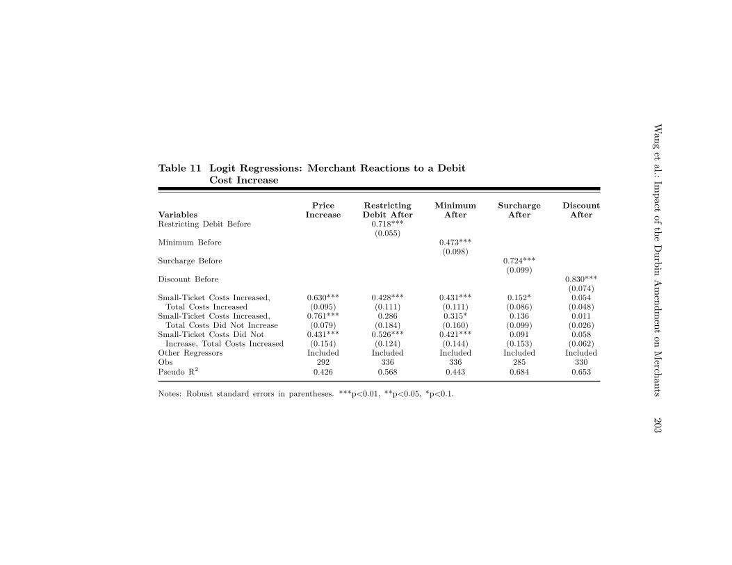
Table 11 reports the coe¢ cient estimates. Again, the results showmerchants�debit restriction policies are persistent. If a merchant im-posed debit restrictions (or speci�cally, minimum amount, surcharge,or discount) prior to the regulation, it is likely the merchant wouldcontinue to do so post-regulation. Table 12 reports the estimated prob-abilities. Holding other explanatory variables at their mean values, if amerchant imposed any debit restrictions prior to the regulation, thereis a 78.2 percent chance the merchant will continue to restrict debit usepost-regulation. Otherwise, the chance is only 6.46 percent. A similarpattern is found for each of the three speci�c restrictions.
More interestingly, the results in Table 11 show that debit costincreases have signi�cant e¤ects on increasing merchants� prices anddebit restrictions. Table 12 reports the estimated probabilities. Hold-ing other explanatory variables at their mean values, if a merchant hadno change for either the total debit costs or the small-ticket costs, thereis only a 5.1 percent chance that the merchant would raise prices. How-ever, if a merchant belongs to the group �small-ticket costs increased,total costs increased,� the chance rises to 59.6 percent; for the group�small-ticket costs increased, total costs did not increase,�the chanceis 74.7 percent; and for the group �small-ticket costs did not increase,total costs increased,�the chance is 33.1 percent. In other words, mer-chants in our sample are likely to pass along their increased debit coststo prices.
Similarly, the results show that merchants in our sample are likelyto increase debit restrictions in reaction to debit cost increases. Ac-cording to Table 12, holding other explanatory variables at their meanvalues, if a merchant had no change for either total debit costs or small-ticket costs, there is only a 17 percent chance that the merchant wouldrestrict debit use post-regulation. However, if a merchant belongs to thegroup �small-ticket costs increased, total costs increased,� the chancerises to 57.3 percent; for the group �small-ticket costs increased, totalcosts did not increase,� the chance is 41.4 percent; and for the group�small-ticket costs did not increase, total costs increased,�the chance is68.1 percent. Moreover, most of the e¤ects are found working throughthe minimum amount requirement, and to a less extent, through sur-charging.
Wangetal.:
Impact
oftheDurbinAmendmentonMerch
ants
203
Table 11 Logit Regressions: Merchant Reactions to a DebitCost Increase
Price Restricting Minimum Surcharge DiscountVariables Increase Debit After After After AfterRestricting Debit Before 0.718***
(0.055)Minimum Before 0.473***
(0.098)Surcharge Before 0.724***
(0.099)Discount Before 0.830***
(0.074)Small-Ticket Costs Increased, 0.630*** 0.428*** 0.431*** 0.152* 0.054Total Costs Increased (0.095) (0.111) (0.111) (0.086) (0.048)
Small-Ticket Costs Increased, 0.761*** 0.286 0.315* 0.136 0.011Total Costs Did Not Increase (0.079) (0.184) (0.160) (0.099) (0.026)
Small-Ticket Costs Did Not 0.431*** 0.526*** 0.421*** 0.091 0.058Increase, Total Costs Increased (0.154) (0.124) (0.144) (0.153) (0.062)
Other Regressors Included Included Included Included IncludedObs 292 336 336 285 330Pseudo R2 0.426 0.568 0.443 0.684 0.653
Notes: Robust standard errors in parentheses. ***p<0.01, **p<0.05, *p<0.1.

204Federal
Reserve
Bank
ofRichm
ondEconom
icQuarterly
Table 12 Merchant Reactions to a Debit Cost Increase(Estimated Probabilities)
Price Restricting Minimum Surcharge DiscountVariables Increase Debit After After After AfterDidn�t Have Restriction/Minimum/ 0.065*** 0.079*** 0.004 0.007Surcharge/Discount Before (0.020) (0.020) (0.004) (0.005)
Had Restriction/Minimum/ 0.782*** 0.551*** 0.728*** 0.836***Surcharge/Discount Before (0.049) (0.094) (0.099) (0.072)
Small-Ticket Costs Increased, 0.596*** 0.573*** 0.451*** 0.119* 0.061Total Costs Increased (0.103) (0.100) (0.102) (0.068) (0.043)
Small-Ticket Costs Increased, 0.747*** 0.414** 0.309** 0.086 0.022Total Costs Did Not Increase (0.106) (0.171) (0.137) (0.053) (0.023)
Small-Ticket Costs Did Not 0.331** 0.681*** 0.415*** 0.057 0.059Increase, Total Costs Increased (0.131) (0.144) (0.135) (0.085) (0.056)
Small-Ticket Costs Did Not Increase, 0.051*** 0.170*** 0.075*** 0.008 0.014Total Costs Did Not Increase (0.017) (0.037) (0.020) (0.007) (0.010)
Other Regressors At mean At mean At mean At mean At meanObs 292 336 336 285 330
Notes: Standard errors in parentheses. ***p<0.01, **p<0.05, *p<0.1.

Wang et al.: Impact of the Durbin Amendment on Merchants 205
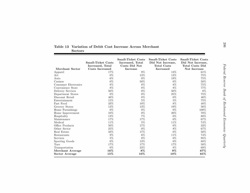
In comparison with the analysis on merchants who had a decreaseof debit costs, the data show more variation of merchants who had debitcost increases. Table 13 shows a decent size of observations in each ofthe groups that involve debit cost increases. Speci�cally, among the 362one-sector merchants in the sample, 16 percent reported �small-ticketcosts increased, total costs increased�; 8 percent reported �small-ticketcosts increased, total costs did not increase�; and 9 percent reported�small-ticket costs did not increase, total costs increased.�
Merchant Reactions: Additional Discussions
Our analysis suggests asymmetric merchant reactions to changing debitcosts. On the one hand, few merchants in our sample are found toreduce prices or debit restrictions as their debit costs decrease. This isalso related to the fact that a relatively small fraction of merchants inour sample reported a decrease of their debit costs in the �rst place.On the other hand, a sizable fraction of merchants are found to raiseprices or debit restrictions as their debit costs increase. Then, a naturalquestion is: What can explain the asymmetry of merchant reactions?
There might be several possibilities. First, our analysis is basedon a relatively small sample. While the survey is intended to capturea diversi�ed set of merchants, there is no guarantee that the sampleis fully representative. Also because the survey is voluntary, it couldbe possible that the survey oversampled merchants who were adverselya¤ected by the regulation.
Second, it is not entirely clear how the survey respondents treatedin�ation or other sector-speci�c factors that may have in�uenced theprice changes. To address the issue, the survey explicitly asked re-spondents whether their prices were increased, decreased, or not af-fected because of Durbin. Presumably, the respondents should teaseout any non-Durbin factors that may have a¤ected prices. However,it could still be possible that some respondents may not be able toperfectly identify price changes solely due to the regulation. Therefore,it would be useful if we could control for price changing factors otherthan Durbin if that data is available.
Third, merchants may indeed have asymmetric reactions to costchanges. In fact, it is a well-documented fact that retail prices tendto respond faster to input cost increases than to decreases (Peltz-man 2000). However, since the survey was conducted two years post-regulation, the asymmetric adjustment speed does not seem to provide
206Federal
Reserve
Bank
ofRichm
ondEconom
icQuarterly
Table 13 Variation of Debit Cost Increase Across MerchantSectors
Small-Ticket Costs Small-Ticket Costs Small-Ticket CostsSmall-Ticket Costs Increased, Total Did Not Increase, Did Not Increase,Increased, Total Costs Did Not Total Costs Total Costs Did
Merchant Sector Costs Increased Increase Increased Not IncreaseApparel 17% 9% 13% 61%Art 0% 13% 13% 75%Auto 6% 0% 19% 75%Casinos 0% 50% 0% 50%Consumer Electronics 8% 8% 8% 75%Convenience Store 8% 8% 8% 77%Delivery Services 50% 0% 50% 0%Department Stores 0% 0% 25% 75%Discount Retail 46% 8% 0% 46%Entertainment 15% 5% 5% 75%Fast Food 33% 10% 8% 48%Grocery Stores 13% 13% 19% 56%Home Furnishings 0% 0% 0% 100%Home Improvement 10% 0% 20% 70%Hospitality 13% 7% 0% 80%Maintenance 17% 17% 0% 67%Medical 11% 5% 11% 74%O¢ ce Products 50% 17% 0% 33%Other Sector 25% 0% 8% 67%Real Estate 33% 17% 0% 50%Restaurants 9% 6% 11% 74%Services 5% 0% 0% 95%Sporting Goods 0% 13% 0% 88%Toys 17% 17% 17% 50%Transportation 0% 23% 8% 69%Merchant Average 16% 8% 9% 67%Sector Average 15% 10% 10% 65%
Wang et al.: Impact of the Durbin Amendment on Merchants 207
an adequate explanation.9
Finally, it is possible that merchants may also engage in non-pricecompetitions. Therefore, in reaction to a cost reduction, merchantsmay not necessarily reduce prices but could instead adjust other mar-gins such as providing better quality of services. Of course, these areall conjectures that require further research.
5. CONCLUSION
In this article, we investigate empirical evidence from a merchant surveyconducted two years after the debit interchange regulation, introducedby the Durbin Amendment to the Dodd-Frank Act, took e¤ect.
The survey results suggest that the regulation has had a limitedand unequal impact on merchants�debit acceptance costs. The ma-jority of merchants in the survey sample (about two-thirds) reportedno change or did not know the change of debit costs post-regulation.Some merchants (about a quarter) reported an increase of debit costs,especially for small-ticket transactions. The remaining less than 10percent of merchants reported a decrease of debit costs. The impactvaries substantially across di¤erent merchant sectors.
We also �nd asymmetric merchant reactions in terms of changingprices and debit restrictions. A sizable fraction of merchants are foundto raise prices or debit restrictions as their costs of accepting debitcards increase. However, few merchants are found to reduce prices ordebit restrictions as debit costs decrease. Further research is needed tounderstand the asymmetric reactions.
REFERENCES
Bedre-Defolie, Özlem, and Emilio Calvano. 2013. �Pricing PaymentCards.�American Economic Journal: Microeconomics 5(August): 206�31.
9 Yang and Ye (2008) develop a model of search with learning to explain this phe-nomenon of asymmetric price adjustments. They show that, when a positive cost shockoccurs, all the searchers immediately learn the true state; the search intensity, and hencethe prices, fully adjust in the next period. When a negative cost shock occurs, it takeslonger for nonsearchers to learn the true state, and the search intensity increases grad-ually, leading to a slow falling of prices.
208 Federal Reserve Bank of Richmond Economic Quarterly
Kay, Benjamin S., Mark D. Manuszak, and Cindy M. Vojtech. 2014.�Bank Pro�tability and Debit Card Interchange Regulation: BankResponses to the Durbin Amendment.�Federal Reserve Board ofGovernors Finance and Economics Discussion Series 2014-77.
Peltzman, Sam. 2000. �Prices Rise Faster than They Fall.�Journal ofPolitical Economy 108 (June): 466�502.
Rochet, Jean-Charles, and Jean Tirole. 2002. �Cooperation amongCompetitors: Some Economics of Payment Card Associations.�RAND Journal of Economics 33 (Winter): 549�70.
Rochet, Jean-Charles, and Jean Tirole. 2011. �Must-Take Cards:Merchant Discounts and Avoided Costs.�Journal of the EuropeanEconomic Association 9 (June): 462�95.
Wang, Zhu. 2010. �Market Structure and Payment Card Pricing:What Drives the Interchange?�International Journal ofIndustrial Organization 28 (January): 86�98.
Wang, Zhu. 2012. �Debit Card Interchange Fee Regulation: SomeAssessments and Considerations.�Federal Reserve Bank ofRichmond Economic Quarterly 98 (Third Quarter): 159�83.
Wang, Zhu. 2014. �Demand Externalities and Price Cap Regulation:Learning from the U.S. Debit Card Market.�Federal ReserveBank of Richmond Working Paper 13-06R.
Wright, Julian. 2003. �Optimal Card Payment Systems.�EuropeanEconomic Review 47 (August): 587�612.
Wright, Julian. 2012. �Why Payment Card Fees Are Biased AgainstRetailers.�RAND Journal of Economics 43 (Winter): 761�80.
Yang, Huanxing, and Lixin Ye. 2008. �Search with Learning:Understanding Asymmetric Price Adjustments.�RAND Journalof Economics 39 (Summer): 547�64.
Economic Quarterly� Volume 100, Number 3� Third Quarter 2014� Pages 209�240
How CanConsumption-BasedAsset-Pricing ModelsExplain Low Interest Rates?
Felipe Schwartzman
The Great Recession gave way to a period of very low short-termnominal and real interest rates. As the recovery proceeds andthe Federal Reserve starts to decide the rhythm with which it
intends to raise policy rates, one fundamental question is whether thelow interest rates are just a symptom of a recessionary period (even ifprolonged) in which the Federal Reserve chose to take a deliberately ex-pansionary stance, or if they re�ect longer-run fundamental forces thatmay not dissipate easily. In the latter case, optimal policy may war-rant a slow increase of the policy interest rate, so that it remains low byhistorical standards even when in�ation and the labor market are closeto their long-run levels. Currently, Federal Open Market Committeemembers appear to forecast such a slow increase, as documented in theSummary of Economic Projections.
The purpose of this article is to use consumption-based asset-pricingmodels to gain some insight into the determinants of the �natural in-terest rate,�that is, the interest rate that would prevail in the absenceof nominal rigidities. Since this natural rate is not itself a function ofcentral bank decisions, it can be used as a yardstick for the stance ofmonetary policy. In particular, in terms of modern monetary theory(Woodford 2003), one can say that the policy stance is expansionary
The author thanks Alex Wolman, Marianna Kudlyak, Pierre-Daniel Sarte, andSteven Sabol for valuable comments that helped improve this article. The viewsexpressed in this article are those of the author and do not necessarily re�ect thoseof the Federal Reserve Bank of Richmond or the Federal Reserve System. E-mail:[email protected].
210 Federal Reserve Bank of Richmond Economic Quarterly
if the interest rate is below the �natural rate of interest�and contrac-tionary otherwise.1 The question about the optimal pace of interestrate lifto¤ can thus be recast in terms of the speed with which thenatural rate of interest is likely to increase.
Consumption-based asset-pricing models are a natural starting pointfor the discussion of the fundamental determinants of interest rates formacroeconomists since they share conventional assumptions of mostworkhorse macroeconomic models: rational expectations, frictionlessasset markets, and a representative household. This contrasts withbehavioral economics models, which emphasize departures from ratio-nal expectations, and with segmented markets models, in which assetprices are determined by only a subset of households.2 While these al-ternatives are certainly worthy of further discussion, the purpose of thisarticle is to provide a �rst look at the progress that one can make withthis more familiar baseline.3 I will review three main strands within theconsumption-based asset-pricing literature: habit formation, long-termrisk, and disaster risk. Rather than provide a comprehensive review ofthe literature within each of those strands, I will discuss some of themain ideas based on a small number of in�uential articles.4 At the endof each section I include a short discussion of how the model could beused to explain low interest rates. Those discussions are meant to beillustrative rather than conclusive, in that they delimit promising ar-eas for further research rather than provide a complete answer to howwell consumption-based asset-pricing models can explain currently lowinterest rates.
As we will see in the models reviewed, interest rates can be loweither because market participants expect consumption growth to below, because they perceive consumption risk to be high, or because
1 Naturally, the central bank chooses the nominal interest rate, with the real interestrate being determined endogenously, whereas the �natural� rate of interest is typicallyunderstood to be a real rate. For more on the link between real and nominal interestrates from a consumption-based asset-pricing perspective, see Sarte (1998) and Wolman(2006).
2 In particular, Mehra and Prescott (2008) question the assumption about whetherthe highly liquid Treasury bill rate is an appropriate measure of the interest rate thathouseholds use to save for retirement and smooth consumption.
3 For examples of articles relying on segmented markets to account for the reductionin interest rates post-2008, see Del Negro et al. (2010), Guerrieri and Lorenzoni (2011),and Eggertson and Krugman (2012), and more generally, Vissing-Jørgensen (2002) andVissing-Jørgensen and Attanasio (2003) for a discussion of how market segmentationa¤ects interest rates. Seminal articles in the behavioral �nance literature are Barberis,Shleifer, and Vishny (1998); Daniel, Hirshleifer, and Subrahmanyam (1998); and Hongand Stein (1999). See also Shleifer (2000) and Barberis and Thaler (2003) for reviews.
4 In fact, to a large extent the material in this article is a reorganization of materialin more detailed reviews by Campbell (2003), Barro and Ursúa (2011), and Cochrane(2011). While this article is written so as to be largely self-contained, the reader isreferred to those texts for many of the details (including some of the derivations).

F. Schwartzman: Consumption-Based Asset-Pricing Models 211
Figure 1 The Equity Premium and the Risk-Free Rate
they have low risk tolerance. In contrast, equity risk premia do notdepend on expected consumption growth. Hence, one can gain someinsight into the driving force behind low interest rates by examiningthe behavior of the risk premium. The evolution over time in the twovariables can be seen in Figure 1. It depicts the postwar values of thereal interest rate, measured by the 30-day Treasury bill rate de�atedby the consumer price index, and of the equity risk premium, both ofwhich averaged over various �ve-year periods.5 The �ve years sincethe onset of the Great Recession stand out not only because of theexceptionally low real rate of interest, but also because of a historicallyhigh equity risk premium. Given the models reviewed, the high riskpremium suggests that low interest rates in the recent period are likelyto be either a consequence of a perception that consumption risk isparticularly high, or of very low risk tolerance.
The article is structured as follows: In the following section, I layout the notation used in the article as well as common conventions,simpli�cations, and approximations. Each subsequent section discusses
5 To calculate the equity risk premium, I use the value weighted equity returnsindex from the Center for Research in Security Prices.
212 Federal Reserve Bank of Richmond Economic Quarterly
one variety of consumption-based asset-pricing models: the Mehra andPrescott (1985) benchmark, the recursive utility and long-run risk ex-tensions of Weil (1989) and Bansal and Yaron (2004), the disaster-riskmodel of Rietz (1988) and Barro (2006), and Campbell and Cochrane�s(1999) habit-formation models. The �nal section concludes.
1. NOTATION, CONVENTIONS, SIMPLIFICATIONS,AND APPROXIMATIONS
Assets are claims on streams of dividends. In particular, purchasingsome asset, i, provides an economic agent with a stochastic stream ofdividends
�Dit+s
1s=0
for as long as the agent holds it. In consumption-based asset-pricing models there are no liquidity constraints or othertransaction costs, so agents can trade assets freely at each period. Ifthe price of asset i is given by P it , then we can de�ne its return betweenperiods t and t+ 1 as
Ri;t+1 �Pi;t+1 +Di;t+1
Pi;t: (1)
Asset pricing concerns itself either with determining the price-dividend ratio for an asset, P
it
Dit; or its expected returns, Et [Ri;t+1]. Typ-
ically, higher returns are associated with lower price-dividendratios.
While the literature discusses the pricing of many kinds of assets,the three main ones are the risk-free asset, a market portfolio of equities,and total wealth. The risk-free asset (denoted by i = f) is exactly whatthe name implies: an asset that pays the same dividend in all states ofnature. As an empirical matter, the asset-pricing literature identi�esthe risk-free asset with short-term Treasury bills. Thus, the predictionsof the models under review for the risk-free rate are going to be themost relevant ones for the purpose of monetary policy analysis.
The market portfolio of equities (i = e) refers to a well-diversi�edportfolio of shares issued by �rms and traded in stock markets withprices summarized by indices such as the S&P 500. This is, in turn,di¤erent from total wealth (i = w), which is a �ctitious asset (in thesense that there are no formal markets for it) that pays out aggre-gate consumption as dividends. It includes equity, bonds, housing, andhuman capital. Oftentimes studies of equity pricing at �rst identifyequity with the wealth portfolio and then in re�nements treat the twoas distinct. The distinction between equity and the wealth portfolionormally focuses on the fact that �rms are leveraged, both becausethey issue bonds and because salaries are normally insulated from
F. Schwartzman: Consumption-Based Asset-Pricing Models 213
high-frequency �uctuations in output. Therefore, for any change in-crease in aggregate endowment, dividends should change by a greateramount. The simplest way of modeling this leverage is to assume thataggregate dividends on equity are a deterministic function of consump-tion, with De
t = (Dwt )
� = C�t , for some � > 1.One simpli�cation used by the asset-pricing literature to obtain
analytical results is to rely on log normality assumptions. If the log ofasset returns is normally distributed, one can use the fact that for anynormally distributed x, E [ex] = eE[x]+
12V ar[x]. Thus, if returns Ri;t+1
are log-normally distributed,
ln (E [Ri;t+1]) = E [ri;t+1] +1
2V ar [ri;t+1] ;
where we use small letters to denote the natural logarithm.A further simpli�cation, used in disaster models, is the use of a
continuous time formulation to study disaster risk. Denote by dt thelength of a period of time. Let eri;t+1dt be the gross return per periodof time of that asset. Suppose the return on some asset i is either e�rdt
with probability e�pdt or (1� b) e�rdt with probability 1� e�pdt. Then
Eheri;t+dtdt
i=he�pdt +
�1� e�pdt
�(1� b)
ie�r:
Taking logs and dividing by dt yields
lnE�eri;t+dtdt
�dt
= �r +ln�e�pdt +
�1� e�pdt
�(1� b)
�dt
:
Taking the limit as dt! 0 and applying l�Hopital�s rule,
E [ri;t+dt] = �r � pb:
The continuous time approximation yields an intuitive expressionfor expected log returns. Those are equal to �r, except that with prob-ability p they fall by b.
Finally, a common approximation used in the analytical literatureis to log-linearize equation (1) to obtain
ri;t+1 = �pi;t+1 + (1� �) di;t+1 � pi;t;
where � is the average PP+D ratio and is typically calibrated to some
value close to 1. Rearranging and iterating forward up to some timet+ T with T > 0 yields
214 Federal Reserve Bank of Richmond Economic Quarterly
pi;t � di;t =TXs=0
�s�dt+1+s �TXs=0
�sri;t+1+s + �T+1pi;T+1:
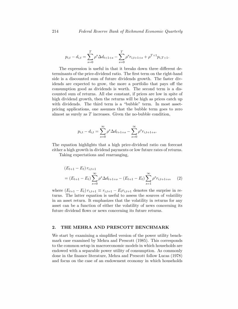
The expression is useful in that it breaks down three di¤erent de-terminants of the price-dividend ratio. The �rst term on the right-handside is a discounted sum of future dividends growth. The faster div-idends are expected to grow, the more a portfolio that pays o¤ theconsumption good as dividends is worth. The second term is a dis-counted sum of returns. All else constant, if prices are low in spite ofhigh dividend growth, then the returns will be high as prices catch upwith dividends. The third term is a �bubble� term. In most asset-pricing applications, one assumes that the bubble term goes to zeroalmost as surely as T increases. Given the no-bubble condition,
pi;t � di;t =1Xs=0
�s�dt+1+s �1Xs=0
�sri;t+1+s:
The equation highlights that a high price-dividend ratio can forecasteither a high growth in dividend payments or low future rates of returns.
Taking expectations and rearranging,
(Et+1 � Et) ri;t+1
= (Et+1 � Et)1Xs=0
�s�dt+1+s � (Et+1 � Et)1Xs=1
�sri;t+1+s; (2)
where (Et+1 � Et) ri;t+1 � ri;t+1 � Etri;t+1 denotes the surprise in re-turns. The latter equation is useful to assess the sources of volatilityin an asset return. It emphasizes that the volatility in returns for anyasset can be a function of either the volatility of news concerning itsfuture dividend �ows or news concerning its future returns.
2. THE MEHRA AND PRESCOTT BENCHMARK
We start by examining a simpli�ed version of the power utility bench-mark case examined by Mehra and Prescott (1985). This correspondsto the common setup in macroeconomic models in which households areendowed with a separable power utility of consumption. As commonlydone in the �nance literature, Mehra and Prescott follow Lucas (1978)and focus on the case of an endowment economy in which households

F. Schwartzman: Consumption-Based Asset-Pricing Models 215
consume and trade claims on immediately perishable fruits that fallfrom an in�nitely lived tree.6
Individual households determine how much to consume in each pe-riod of time and how much to invest in a portfolio of assets that ithas available. We assume that there are N di¤erent assets, indexedi 2 f1; :::; Ng, and that those assets completely span the shocks thatthe households are subject to so that markets are complete. The prob-lem of the household is
maxfxitg(1;N)
(t;i)=(0;1)
E0
" 1Xt=0
�tC1� t � 11�
#
s:t: : Ct +
NXi=1
Pi;txi;t =
NXi=1
xi;t�1 (Pi;t +Di;t) ;
where xit is the amount of shares of asset i held by the household at timet and, as before, P it is the realized price and D
it is its realized dividend.
The parameter is the coe¢ cient of relative risk aversion and governsthe tolerance that households have for risk. It is also the inverse ofthe intertemporal elasticity of substitution, governing the household�sdesire to smooth consumption over time. The optimality condition forthe household is
Pi;tC� t = �Et
hC� t+1 (Pi;t+1 +Di;t+1)
i:
Let Ri;t+1 � Pi;t+1+Di;t+1Pi;t
be the return on asset i. Returns, like prices,are equilibrium objects determined endogenously. Given expected fu-ture prices and dividends, higher returns are tied to lower prices at t.Given the de�nition of returns and the optimality condition, we havethat
1 = �Et
"�Ct+1Ct
�� Ri;t+1
#: (3)
The ratio of marginal utilities�Ct+1Ct
�� is the pricing kernel in
this economy. In order to hold a positive and �nite amount of an
6 The analysis of asset-pricing models to environments with production (�Produc-tion Based Asset Pricing�) is itself an active area of research that we will leave undis-cussed. For important contributions in that literature, see Cochrane (1991); Jermann(1998); Boldrin, Christiano, and Fisher (2001); and Gomes, Kogan, and Zhang (2002),among many others.
216 Federal Reserve Bank of Richmond Economic Quarterly
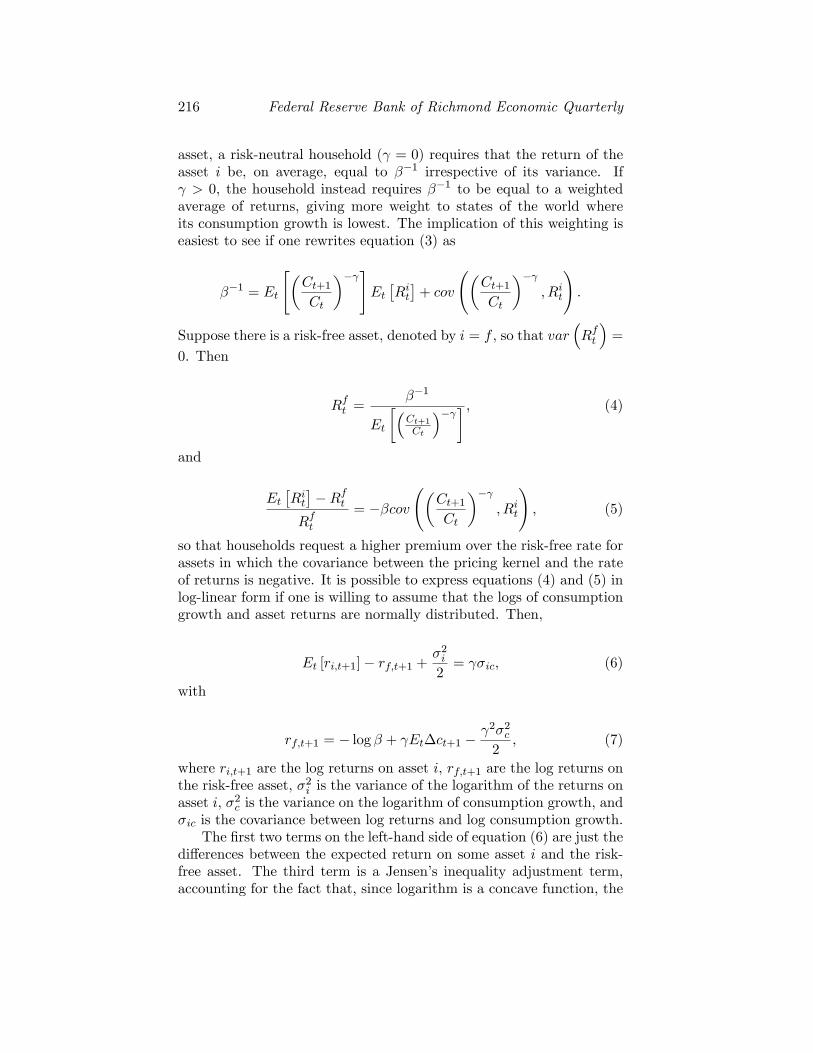
asset, a risk-neutral household ( = 0) requires that the return of theasset i be, on average, equal to ��1 irrespective of its variance. If > 0, the household instead requires ��1 to be equal to a weightedaverage of returns, giving more weight to states of the world whereits consumption growth is lowest. The implication of this weighting iseasiest to see if one rewrites equation (3) as
��1 = Et
"�Ct+1Ct
�� #Et�Rit�+ cov
�Ct+1Ct
�� ; Rit
!:
Suppose there is a risk-free asset, denoted by i = f , so that var�Rft
�=
0. Then
Rft =��1
Et
��Ct+1Ct
�� � ; (4)
and
Et�Rit��Rft
Rft= ��cov
�Ct+1Ct
�� ; Rit
!; (5)
so that households request a higher premium over the risk-free rate forassets in which the covariance between the pricing kernel and the rateof returns is negative. It is possible to express equations (4) and (5) inlog-linear form if one is willing to assume that the logs of consumptiongrowth and asset returns are normally distributed. Then,
Et [ri;t+1]� rf;t+1 +�2i2= �ic; (6)
with
rf;t+1 = � log � + Et�ct+1 � 2�2c2
; (7)
where ri;t+1 are the log returns on asset i, rf;t+1 are the log returns onthe risk-free asset, �2i is the variance of the logarithm of the returns onasset i, �2c is the variance on the logarithm of consumption growth, and�ic is the covariance between log returns and log consumption growth.
The �rst two terms on the left-hand side of equation (6) are just thedi¤erences between the expected return on some asset i and the risk-free asset. The third term is a Jensen�s inequality adjustment term,accounting for the fact that, since logarithm is a concave function, the
F. Schwartzman: Consumption-Based Asset-Pricing Models 217
logarithm of an expected variable is always larger than the expectationof the logarithm.7 The term on the right-hand side has two compo-nents. The second, �ic, is the covariance between the asset return andconsumption growth and can be interpreted as the �quantity of risk�in the asset. The �rst, , is the coe¢ cient of relative risk aversion andit can be interpreted as the �price� of risk. Under power utility, theprice of risk is constant, and asset prices only depend on the risk oneperiod ahead.
As famously demonstrated by Mehra and Prescott (1985), the modelperforms poorly in quantitative terms. In their baseline exercise, theyequate equity with the wealth portfolio, i.e., an asset that pays outaggregate consumption as dividends.8 Given that consumption growthdoes not vary much, the quantity of risk �ic is very low. Because of that,Mehra and Prescott �nd that for reasonable values of (10 and under),the equity risk premium implied by the right-hand side of equation (6)is an order of magnitude smaller than the one found in the data. Thisobservation has spurred a very large literature and is a cornerstone ofmodern asset-pricing research.
For a large enough ; the model is of course able to match theequity premium. However, setting to a very large number also hasimplications for the risk-free rate that do not �t the data. In an av-erage quarter, consumption growth Et [�ct+1] is close to 2 percent inyearly terms and the standard deviation has a similar magnitude. Ifwe take the coe¢ cient of risk aversion to be = 10, close to Mehra andPrescott�s upper bound, then matching the risk-free rate of 1 percentin yearly terms would require a discount rate of close to �19 percentper year. In a period of time where expected consumption is 1 percentinstead of 2 percent, the interest rate would fall from 1 percent to �9percent.
Intuitively, the reason for the tradeo¤ between matching the highrisk premium and the low interest rate is that captures how unwillinghouseholds are to let consumption vary, be it over time or betweenstates of nature. The higher , the more households dislike variation inconsumption along either dimension. Hence, if a household with a high foresees that its consumption will grow slower, it will be very willingto borrow in order to keep consumption smoothed out over time. Inequilibrium, this leads to a sharp reduction in the interest rate.
7 Formally, Jensen�s inequality states that if g is a concave (convex) function, then
g (E [x]) > (<) E [g (x)]. In that speci�c case, the left-hand side is log�EhRi;t+1Rf;t+1
i�>
Ehlog
hRi;t+1Rf;t+1
ii= Et [ri;t+1]� rf;t+1.
8 As a robustness, they also consider the case where leverage increases the volatilityof equities.

218 Federal Reserve Bank of Richmond Economic Quarterly
Figure 2 Consumption Growth and Risk
Implications for the Interest Rate in theRecent Period
While, in quantitative terms, the Mehra and Prescott benchmark failsas an explanation of asset pricing, it is still a useful benchmark inthat it highlights which factors are likely to matter for interest ratesin consumption-based asset-pricing models. In what follows, I use thisbenchmark as a qualitative guide to the factors driving the risk-freeinterest rate and show how they have evolved in the current recession.For convenience, I restate equation (6) for the risk-free rate below:
rf;t+1 = � log � + Et�ct+1 � 2�2c2
: (8)
As equation (8) makes clear, interest rates can either be low becausemarket participants expect consumption growth to be low or becausethey perceive consumption risk to be high.
Figure 2 shows the average and standard deviations of quarterlyconsumption growths, both expressed in annualized terms and averaged
F. Schwartzman: Consumption-Based Asset-Pricing Models 219
over various �ve-year periods.9 While 2009�13 does feature exception-ally low consumption growth for historical standards, it also featuresexceptionally low consumption variance. Hence, in qualitative terms,the model would have to account for the low interest rates through lowexpected consumption growth.
It is worth highlighting that, given the Mehra and Prescott (1985)benchmark, there is a tension between Figures 1 and 2, since equation(6) implies that, if consumption is correlated with dividends, a highvariance of consumption growth ought to be associated with a highequity premium.10 In contrast, we observe a low variance of consump-tion growth and a high equity premium. As we will see, alternativeconsumption-based asset-pricing models can provide potential resolu-tions to this inconsistency, as they allow either for the possibility thatthe �price�of risk may be changing (as in habit formation models) orthat the kind of short-term consumption risk depicted in Figure 2 maynot be the best measure of the kind of risk that asset holders are mostlyconcerned with when making their portfolio decisions.
3. RECURSIVE UTILITY AND LONG-RUN RISK
As discussed above, a major challenge facing common power-utilitymodels is the di¢ culty in matching both households�willingness to lettheir consumption change over time (captured by a low interest rate)and their unwillingness to let it vary across states of nature (capturedby the high equity risk premium). One possible solution to this ten-sion is to allow for the possibility that the desire for intertemporalsmoothing is governed by a di¤erent parameter than the desire for in-surance. This is provided by the recursive utility function proposed byEpstein and Zin (1989) and Weil (1989, 1990), based on prior work byKreps and Porteus (1978). In particular, the recursive utility function
9 The consumption series is taken from Martin Lettau�s website and is de�nedin Lettau and Ludvigson (2001). In particular, it excludes durable goods, shoes, andclothing.
10 Consumption variance is an important factor in explaining the equity risk pre-mium under the assumption that that consumption growth is i.i.d. and that growth instock dividends is perfectly correlated with consumption growth, so that �de;t = ��ce;t.Then, if we guess that equity returns are also i.i.d., from equation (2) we have that
(Et+1 � Et) re;t+1 = (Et+1 � Et)�dt+1:
Since dividend growth is i.i.d., the guess that equity returns are i.i.d. is veri�ed. In thiscase, the covariance between consumption and equity returns �ec is simply �var (�ce;t).Hence, from equation (6), higher consumption variance is associated with a higher equityrisk premium.

220 Federal Reserve Bank of Richmond Economic Quarterly
provides for the representation of preferences over lotteries in whichagents rank them in terms of the time in which uncertainty is resolved.For example, an agent may face two di¤erent lotteries that pay thesame amounts at some distant date depending on the �ip of a coin,but in one lottery the coin �ip takes place immediately, whereas in theother it only takes place much later. Under this kind of preference,agents may prefer the �rst lottery to the second even though the distri-bution of outcomes is identical.11 The Epstein-Zin-Weil (EZW) utilityfunction can be written as
Ut =
((1� �) [Ct]1�
1 + �
��EtU
1� t+1
� 11� �1� 1
) 1
1� 1
; (9)
where Ut is the utility at time t. Preferences for early resolution ofuncertainty emerge if 1 < .
The parameter can be interpreted as the intertemporal elasticityof substitution. This interpretation becomes most clear in the deter-ministic case. Without uncertainty, the exponents in 1� around Ut+1cancel out and, with a slight rearrangement, equation (9) collapses tothe usual Bellman equation format, with period utility of consumption
given by C1� 1
t .The parameter can be interpreted as a risk-aversion parameter.
Heuristically, this can be seen in a version of the problem where thehousehold only consumes in t = 2 so that there are no intertemporalchoices to be made. Then, Ut = 0 for t > 2, U2 = C2; and U1 =
�1
1� 1 Et
hC1� 2
i 11� , so that the problem of the household is equivalent
to maximizing expected utility EthC1� 2
i.12
Finally, it is also straightforward to check that, if 1 = , equation(9) collapses back to a recursive version of the benchmark power-utilitycase, in which the coe¢ cient of relative risk aversion is equal to theinverse of the intertemporal elasticity of substitution.
Given this utility function, one can derive the following Euler equa-tion for portfolio decisions:13
11 This is a violation of the independence axiom for preferences so that withEpstein-Zin-Weil preferences, utility will not necessarily be separable across states ofnature.
12 Stictly speaking, for this example we would need < 1, so that the utility func-tion is still well de�ned for Ct = 0.
13 See the Appendix for a derivation.
F. Schwartzman: Consumption-Based Asset-Pricing Models 221
1 = Et
24(��Ct+1Ct
�� 1
)� �1
Rw;t+1
�1��Ri;t+1
35 ; (10)
where Rw;t+1 is the return on total household wealth and � � 1� 1� 1
, so
that in the benchmark power-utility case, � = 1. The pricing kernel
is���Ct+1Ct
�� 1
�� �1
Rw;t+1
�1��and is a weighted average of the pric-
ing kernel obtained in the benchmark separable utility case and thereciprocal of the return on wealth, Rw;t+1.The return on wealth in thepricing kernel captures the impact of news about future consumptionon agent�s marginal utility. To see this, recall that, from equation (2),surprises in the returns to the wealth portfolio satisfy
(Et+1 � Et) rw;t+1
= (Et+1 � Et)1Xs=0
�s�ct+1+s � (Et+1 � Et)1Xs=1
�srw;t+1+s; (11)
where we use the fact that, by de�nition, the dividends on the wealthportfolio are equal to aggregate consumption. Thus, surprises to thereturns on wealth re�ect surprises in future consumption growth, dis-counted by surprises to the future returns on wealth itself.
The reason why returns on wealth are factors in the pricing ker-nel under EZW preferences is because of the nonseparability betweenutility for current and future consumption. With power utility, prefer-ences are separable. Given that agents are able to completely changetheir portfolio each period, they need not concern themselves with con-sumption �ows in the far future when evaluating which portfolio tohold between two adjacent periods. This is no longer true with EZWpreferences.
If the logs of consumption growth and returns are normally dis-tributed, we can write the following expression for the risk premiumassociated with any given asset i:
Etri;t+1 � rf;t+1 +�2i2= �
�ic + (1� �)�iw; (12)
and for the risk-free rate,
rf;t+1 = � log � +1
Et [�ct+1] +
� � 12
�2w ��
2 2�2c ; (13)

222 Federal Reserve Bank of Richmond Economic Quarterly
where now �iw is the covariance between the returns on asset i and thereturn on total household wealth, and �2w is the variance of the totalreturns on wealth.
Recursive preferences allow one to account for the equity premiumpuzzle in two ways. First, as highlighted by Weil (1989), there is nolonger a tradeo¤ between matching the equity risk premium and therisk-free rate, as there is an additional parameter to be calibrated.Furthermore, as explored in detail by Bansal and Yaron (2004), with� 6= 1; the covariance of the asset return with the return on total wealth�iw becomes an additional factor in determining the equity premium.Thus, if, for example, the variation in total return on wealth is similar tothe variation in equity returns, then returns on total wealth are clearlymuch more volatile than consumption, so that �iw is potentially muchlarger than �ic.
One problem with evaluating equations (12) and (13) is that thevariance of total wealth is hard to measure since total wealth includeshuman capital. One can make some progress by imposing structure onthe process for consumption. In particular, suppose that the consump-tion growth �ct+1 is the sum of a predictable component zt and anunpredictable one �c;t+1 as in
�ct+1 = zt + �c�c;t+1
zt+1 = (1� �) g + �zt + �z�z;t+1;with �c;t+1 and �z;t+1 i.i.d. standard normal variables.14 With � closeto 1 and high �c, this structure allows for consumption growth to havea predictable, stochastic, long-term component, even if at high frequen-cies overall consumption growth is hard to predict.15 For the wealthportfolio, the dividends are equal to aggregate consumption, so thatRw;t =
Pw;t+1+Ct+1Pw;t
. From equations (12) and (13) we have that, if riskdoesn�t vary over time (so that it is homoscedastic), then
Etrw;t+1 = �+1
Et [�ct+1] ;
where � is a constant that depends on the variances. This allows us tosubstitute out the returns from the right-hand side of equation (2) toobtain
14 It is straightforward but tedious to allow for correlation between �c;t+1 and�z;t+1, so we will assume that they are uncorrelated.
15 The question of whether or not consumption growth rate has a persistent com-ponent is hard to settle, since � is hard to estimate in small samples. Bansal and Yaron(2004) show that a large � is not inconsistent with observed autocovariance of consump-tion growth and observed variances of consumption growth at di¤erent horizons.
F. Schwartzman: Consumption-Based Asset-Pricing Models 223
(Et+1 � Et) rwt+1= (Et+1 � Et)�ct+1+s
+
�1� 1
�(Et+1 � Et)
1Xs=1
�s�ct+1+s: (14)
We can now use the expression just derived to describe the sourcesof one-step-ahead variation in returns to the wealth portfolio. The �rstcomponent on the right-hand side is the innovation in consumptiongrowth, with variance �2c . The second component is a discounted sumof future consumption growth. It changes as news about future con-sumption growth arrives, in the form of innovations to zt+1. This sec-ond component incorporating news about future consumption is whatallows returns on the wealth portfolio, and hence the pricing kernel,to be signi�cantly more volatile than consumption growth. If, instead,consumption growth were i.i.d. so that this component would be equalto zero, the variance of returns on wealth would be as small as the vari-ance of consumption growth. The higher variance of the pricing kernelassociated with persistence in consumption growth is what allows mod-els with EZW preferences to imply substantially larger risk premia thanmodels with power utility for a given value of the risk-aversion para-meter , as one can see from equations (12) and (13) determining therisk premium and the risk-free rate.
Bansal and Yaron (2004) emphasize that a reasonable parameter-ization of the model requires both > 1 and > 1. They choose = 10, at the upper bound of Mehra and Prescott�s (1985) exercise,and = 1:5. The choice of is subject to debate, as many empiri-cal studies of consumption behavior over time point to very low valuesfor . Bansal and Yaron (2004) counter that stochastic variance inconsumption introduces a downward bias in estimates of and that,furthermore, studies with more disaggregated consumption data sup-port lower . Importantly, they also point out that one can disciplinethe value of through the correlation between asset prices and newsabout consumption growth and consumption volatility. This can beseen in equation (14), where, with > 1, news about future consump-tion growth leads to an increase in the returns on wealth, but with < 1 such news leads to a reduction.
As emphasized by Bansal and Yaron (2004), recursive preferencesimply that risk premia vary not only with news about future consump-tion growth, but also with news about its variance. A higher varianceof innovations to future consumption growth increases the variance ofreturns on the wealth portfolio and, hence, of the pricing kernel, lead-ing to a higher equity premium and lower risk-free rates. Therefore,
224 Federal Reserve Bank of Richmond Economic Quarterly
time variation in the variance of long-run growth (�long-run risk�) canbe an important factor explaining the variance in risk premia observedin the data.
Implications for the Interest Rate in theRecent Period
For convenience, I restate the equation describing the determinants ofthe risk-free rate:
rf;t+1 = � log � +1
Et [�ct+1] +
� � 12
�2w ��
2 2�2c :
Note that under the calibration adopted by Bansal and Yaron(2004), 1 =
23 ,
��12 = �14, and �
2 2= �6, so that the weight placed
on the two risk factors is comparatively large. This equation holds forthe case of homoscedastic risk. Bansal and Yaron (2004) also providea derivation of the risk-free rate when risk is time varying so that �2wand �2c are functions of time. In that case, the coe¢ cients change butthe essential factors determining the risk-free rate remain the same.16
The recursive preferences model implies that the risk-free rate changesnot only with the expected growth rate of consumption or with thevariance of that growth rate, but also with changes in the mean andvariance of returns on wealth, �2w. As previously discussed, these are, inturn, functions of the variance of the long-term component of consump-tion growth. Given the calibration advocated by Bansal and Yaron(2004), a reduction in the interest rate could thus stem not only fromthe same factors that explain the reduction in interest rates in thebenchmark time-separable model, but also from an increase in the vari-ance of the long-run component of consumption growth.
Total wealth in the economy includes not only equity in �rms, butalso housing and human capital. Figure 3 depicts the volatilities ofequity returns and house price increases over �ve-year periods.17 Bothvolatilities were high by historical standards in the 2009�13 period,most notably the volatility of housing returns. Thus, long-run riskcould, in principle, help explain the low interest rates while account-ing for the disconnect between high risk premia and the low volatilityof consumption growth in that period. More generally, however, the
16 Bansal and Yaron consider a case in which there is only one stochastic risk factorso that �2w and �2c co-move perfectly.
17 The housing price data is from Shiller (2015). House price increases are a goodapproximation for housing returns so long as rents are stable.
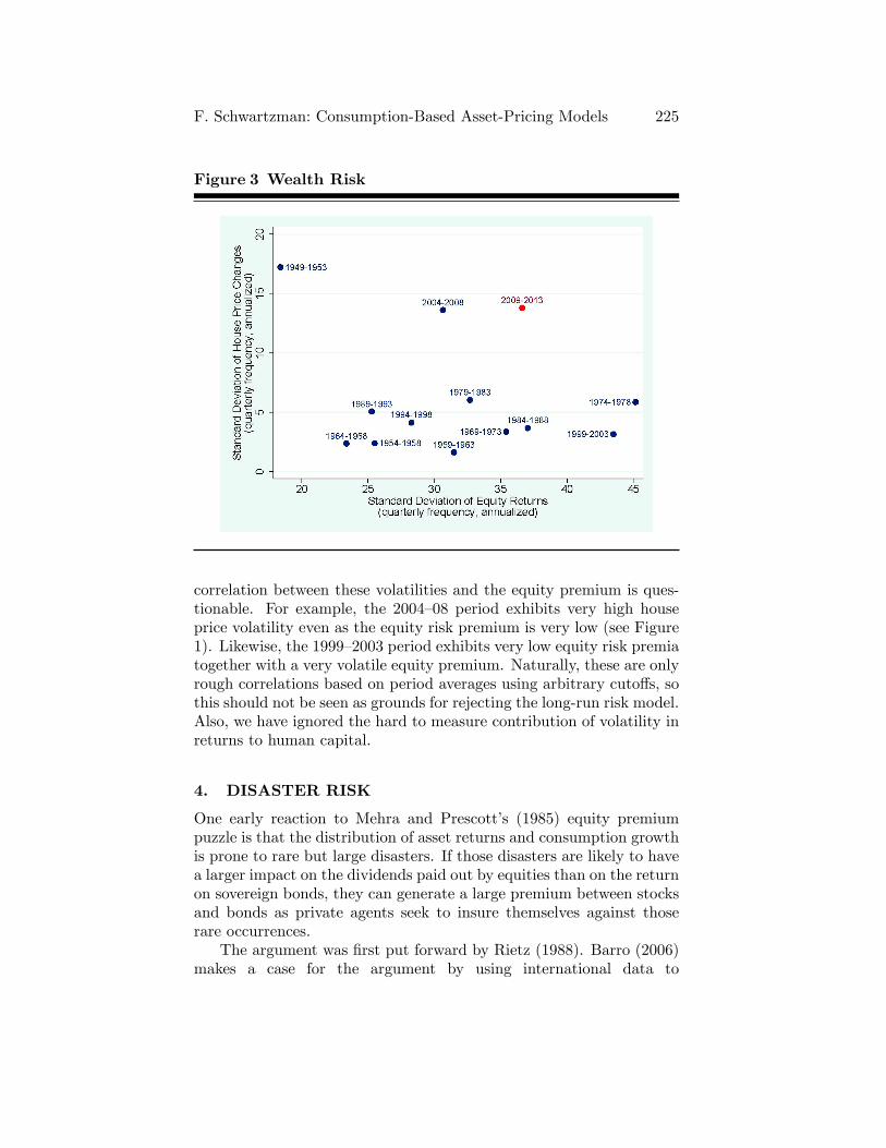
F. Schwartzman: Consumption-Based Asset-Pricing Models 225
Figure 3 Wealth Risk
correlation between these volatilities and the equity premium is ques-tionable. For example, the 2004�08 period exhibits very high houseprice volatility even as the equity risk premium is very low (see Figure1). Likewise, the 1999�2003 period exhibits very low equity risk premiatogether with a very volatile equity premium. Naturally, these are onlyrough correlations based on period averages using arbitrary cuto¤s, sothis should not be seen as grounds for rejecting the long-run risk model.Also, we have ignored the hard to measure contribution of volatility inreturns to human capital.
4. DISASTER RISK
One early reaction to Mehra and Prescott�s (1985) equity premiumpuzzle is that the distribution of asset returns and consumption growthis prone to rare but large disasters. If those disasters are likely to havea larger impact on the dividends paid out by equities than on the returnon sovereign bonds, they can generate a large premium between stocksand bonds as private agents seek to insure themselves against thoserare occurrences.
The argument was �rst put forward by Rietz (1988). Barro (2006)makes a case for the argument by using international data to

226 Federal Reserve Bank of Richmond Economic Quarterly
calculate the probabilities and magnitudes of large disasters, putting a1.7 percent probability of a collapse in consumption of, on average, 30percent.18 He also calculates the probability of sovereign default in theevent of a disaster and the recovery rate that investors can expect inthose events. He �nds that with a coe¢ cient of relative risk aversionas small as four and a discount rate of 3 percent per year, it is possibleto obtain equity premia and risk-free rates that are closer to the data.
Barro (2006, 2009) considers an environment where the aggregateendowment follows a random walk with drift g and variance �2c mostof the time, but with probability p it collapses permanently to a frac-tion 1 � b of its value, where b is itself a random variable drawn fromthe empirical distribution of disasters that he documents. Taking acontinuous-time limit, Barro (2009) arrives at expressions that, after asubstitution, yield the following expressions for the risk-free rate:19
rf = � log � + g � 12 2�2 � p
�E (1� b)� � 1
�;
and, if one takes, as he does, equity to incorporate all of the wealthportfolio, for the risk premium:
re � rf = �2 + phE (1� b)� � E (1� b)1� � E [b]
i:
Thus, an increase in the probability of disasters leads to a reductionin the riskless rate and an increase in the equity risk premium. Oneimportant result is that asset returns are nonlinear functions of thesize of disasters b. This enhances the ability of disasters generatinglarge risk premia and low interest rates since, as b approaches 1; themarginal utility of consumption in the disaster state approaches in�nity.Furthermore, as emphasized by Barro, the model can accommodate�bonanzas,�which are as large as the disasters and still generate largerisk premia, since households will be much more concerned with thedisaster states (in which they have high marginal utility) than with thebonanza states (in which their marginal utility is low).
Barro and Ursúa (2011) provide a comprehensive review of the smallliterature that has emerged around the notion of disaster risk being akey driver of asset-pricing data. This literature has expanded the model
18 In particular, Barro de�nes a disaster as an event in which gross domestic prod-uct (GDP) drops by 15 percent or more, and equate the change in consumption withthe observed change in GDP.
19 The substitution in question is from the expected consumption growth
EthCt+1�Ct
Ct
i(denoted g� in Barro [2009]) for its determinants, g + 1
2�2 � p � E [b].
The substitution singles out g since it is likely to be closer to observed average logconsumption growth then g�.

F. Schwartzman: Consumption-Based Asset-Pricing Models 227
to allow for time-varying disaster risk, thus allowing it to explain time-varying risk premia (Gourio 2010), and disasters that are correlatedacross countries and happen slowly rather than quickly (Nakamura etal. 2010), as well as to evaluate implications of the model for additionalasset pricing facts (Gabaix 2008).
Implications for the Interest Rate in theRecent Period
For convenience, I restate the equation describing the determinants ofthe risk-free rate:
rf = � log � + g � 12 2�2 � p
�E (1� b)� � 1
�:
In addition to the determinants of interest rates in the other models(expected growth and one-step-ahead volatility of consumption), mod-els with economic disasters imply that interest rates ought to changein response to changes in the probability of disaster or to changes inthe expected size of disasters.
It is plausible that, in the aftermath of the Great Recession, eco-nomic agents have updated upward their subjective probabilities ofsuch an episode occurring again. This could go some way in explainingthe smaller interest rate observed in the recent period. In particu-lar, consumption dropped 2.7 percent between Q2:2007 and Q4:2009.Relative to a 2 percent per year trend, the reduction was 7.9 percent.Suppose that, given that observation, agents assign a probability of 5percent to a drop in consumption of 5 percent in any given period, sothat such a disaster occurs on average every 20 years.20 Then, if theyhave a risk aversion of four, they will request a risk-free rate that is0:05
�0:95�4 � 1
�= 1:14 percent in yearly terms smaller than before.
This revision is unlikely to dissipate very quickly since, given the smallprobabilities of a disaster occurring, the fact that another one hasn�tcome to fruition should weigh little on the probability assessment. Im-portantly, apart from helping explain the lower interest rate, the dis-aster risk could allow one in principle to reconcile the low volatility of
20 A 5 percent probability would be high compared to the 1.7 percent calculated byBarro (2006), but, in contrast, the reduction in consumption of 5 percent is less extremethan the average 30 percent reduction found in that study. One obvious caveat is thatthe drop in consumption occurred smoothly, over two and a half years, whereas themodel assumes that the whole change occurs instantaneously. Nakamura et al. (2010)show how the rare disaster model can accomodate slow disasters if agents have EZWpreferences.

228 Federal Reserve Bank of Richmond Economic Quarterly
consumption with the high equity premium in the post-Great Recessionera.
5. HABITS
In both the discussion of rare disasters and long-term risk, the timevariation in expected risk premia is understood primarily as stemmingfrom time variation in the quantity of risk that households face. Underhabit formation, this same time variation is explained as stemmingfrom variation in the risk tolerance of households, which determinesthe price of risk.
In habit-formation models, the marginal utility of consumption de-pends on a time-varying state variable that evolves as a function ofpast consumption decisions. The key idea is that as households be-come habituated to certain consumption levels, their marginal utility ofconsumption becomes higher for a given level of consumption. Habit-formation models di¤er along several dimensions, including whetherhabits are �internal� (where habit depends on individual householdconsumption) or �external� (where habit depends on aggregate con-sumption), whether habits enter in the utility function multiplicativelyor additively, and whether habits change more or less quickly with con-sumption.21 In what follows, we discuss the model by Campbell andCochrane (1999).
Campbell and Cochrane (1999) point out that habit models aresuccessful in generating volatile time-varying risk premia because theyincrease the volatility of the marginal utility of consumption. Theyassume habits enter additively and are �external�so that
u (Ct; Xt) =(Ct �Xt)
1� � 11� ;
where Xt is the stock of habits. Then the curvature of the utilityfunction with respect to Ct is given by
ucc (Ct; Xt)Ctuc (Ct; Xt)
= �
St;
where St � Ct�XtCt
is �surplus consumption,�the gap between consump-tion and the habit. It follows that the curvature is higher in absolute
21 See Campbell (2003) for a more detailed discussion. Models of habits in �nanceinclude Sundaresan (1989), Abel (1990, 1999), Constantinides (1990), and Campbell andCochrane (1999), among others.

F. Schwartzman: Consumption-Based Asset-Pricing Models 229
terms when consumption is closest to its habit level Xt. This time-varying curvature implies that the pricing kernel uc(Ct+1;Xt+1)uc(Ct;Xt)
is alsolikely to vary with St.
To complete the speci�cation of preferences, Campbell and Cochrane(1999) need to specify how habits evolve over time. Rather than usinga more conventional speci�cation in which the habit stock Xt evolvesas a log-linear function of Ct, they recur to a nonlinear speci�cation inwhich St is a log-linear function of changes in log Ct. One advantageof this speci�cation is that it ensures that surplus consumption St isalways positive, which is necessary for the utility to be well de�ned.They de�ne the evolution of surplus consumption to be given by
st+1 = ��s+ (1� �) st�1 + � (st) (ct+1 � ct � E [ct]) ;where �S is the steady-state level of the habit (and �s its log), and � (st)is a nonlinear function of st. The nonlinear term � (st) helps themdeal with one important di¢ culty with habit-formation models. Thisis that, while a time-varying pricing kernel helps generate volatile ex-pected risk premia, it can also give rise to counterfactually volatileinterest rates. In Campbell and Cochrane�s speci�cation, the risk-freerate is given by
rft = � ln (�) + Et [�ct+1]� (1� �) (st � �s)� 2�2
2[1 + � (st)]
2 :
The �rst two terms are the ones obtained in a model without habits.The following two include the e¤ect of habits. The third term summa-rizes the e¤ect of habits on intertemporal substitution. Surplus con-sumption is expected to mean revert at the rate 1��. If it is above itssteady-state levels, then households expect it to become smaller overtime, which is to say that they expect their marginal utility to becomesmaller. Thus, they become more patient, leading to a smaller equi-librium risk-free rate. The last term on the right-hand side capturesthe e¤ect of consumption risk on the risk-free rate. Now, apart fromthe usual reason through which consumption risk generates precau-tionary savings, households also seek to keep their consumption risklow because it is correlated with their habit formation. In periods inwhich realizations of consumption are high, surplus consumption alsoincreases.
Campbell and Cochrane (1999) discipline their choice of � (st) byadding three requirements. Two of them are technical. They imposethat Xt is pre-determined in steady state and that it is always increas-ing in shocks to ct. These conditions ensure that, close to steady state,their process for habits resembles more common speci�cations. The

230 Federal Reserve Bank of Richmond Economic Quarterly
third requirement is that risk-free rates do not vary with habits. Thus,by construction, their model delivers a low volatility for the risk-freerates, as in the data. This allows them to focus more sharply on thevariation in risk premia. Given Campbell and Cochrane�s (1999) cali-bration, the interest rate is
rft+1 = � log (�) + Et [�ct+1]�� �S
�2 �2c2:
Note that �Sis the curvature of the utility function with respect to
consumption in steady state and is thus a measure of the risk toleranceof households. If �S < 1, it is possible for the model to have a largesteady-state curvature with respect to consumption ( �S ), leading tohigh risk premia, even if it has a relatively low . This, in turn, allowsit to admit more moderate interest rates. Speci�cally, Campbell andCochrane calibrate = 2:372 and �S = 0:049, so that the curvature ofthe utility function close to steady state is approximately equal to 48.
Campbell and Cochrane (1995) also consider an extension of themodel in which they choose � (st) to ensure that risk-free rates are alinear function of log habits, decreasing when surplus consumption ishigh. They pick the intercept to correspond to a 1 percent real interestrate and the slope so that the lower bound for the real interest rate iszero.
Implications for the Interest Rate in theRecent Period
For convenience, I restate the equation describing the determinants ofthe risk-free rate:
rft+1 = � log (�) + Et [�ct+1]�� �S
�2 �2c2:
As calibrated by Campbell and Cochrane, the factors determin-ing the real interest rate in the model with habits are the same as inthe Mehra and Prescott (1985) benchmark, the only di¤erence beingthat the model with habits assigns a greater weight to consumptionvolatility.
The models with long-run or disaster risk are able to explain thereduced interest rate with the introduction of risk factors that cannot beeasily discerned by measured consumption volatility. The model withhabits stands in contrast to that. Thus, like the Mehra and Prescott(1985) benchmark, it needs to rely on the historically low consumptiongrowth rate to account for the low interest rates. However, for any
F. Schwartzman: Consumption-Based Asset-Pricing Models 231
choice of , the habit model also puts a greater weight on the variance ofconsumption growth �c (since �S < 1), which was also low by historicalstandards in the post-2009 period. Therefore, for any choice of , thehabit model would imply that the risk-free rate should have fallen byless than what is implied by the Mehra and Prescott (1985) benchmark.
One signi�cant advantage of the habit formation model over theMehra and Prescott model is that it can also accommodate the histor-ically high equity risk premium, since the reduction in consumption inthe aftermath of the Great Recession would have meant that �surplusconsumption�St would be particularly low, leading to increased riskaversion.
6. SUMMARY AND CONCLUSION
The large drop in interest rates following the 2008 recession has givenrise to discussions about whether the reduction was mainly due topolicy or whether policy was following as best it could the �natural�rate and, in the latter case, what the determinants of that reductioncould be. While explanations focusing on market segmentation havegained prominence, asset-pricing models in frictionless environmentsmight also be able to provide sensible explanations for that drop.
In the text above, I discussed, on top of the benchmark power utilityof Mehra and Prescott (1985), three leading varieties of consumption-based asset-pricing models with special focus on the determinants ofthe risk-free rate: long-run risk, disaster risk, and habit formation. Allvariants suggest that interest rates ought to be a function of expectedconsumption growth. This implication is consistent with the fact thatconsumption growth was low by historical standards in the 2009�13period. At the same time, within this period there was a reduction inthe volatility of consumption growth, which could enhance the e¤ect ofthe reduced growth rate.
The challenge for the benchmark Mehra and Prescott (1985) frame-work is that this period also exhibits an equity premium that is highby historical standards, but consumption volatility is small. The threevariants discussed are able to resolve that tension in di¤erent ways.Under long-run risk and disaster-risk models, agents� risk perceptionwould increase because of, respectively, higher variance in the long-run component of consumption growth or a perceived increase in theprobability of a large consumption decrease. The former is consis-tent with historically high equity market volatility, and the latter withan upward revision of the probability of disaster following the GreatRecession. Under the habit-formation model, the tension can poten-tially be resolved by the observation that the reduction in consumption
232 Federal Reserve Bank of Richmond Economic Quarterly
following the Great Recession led to increased risk aversion as house-holds found themselves closer to their �subsistence�level of consump-tion. The explanations based on increased risk diverge from the habitformation in that the same increase in perceived risk that leads to anincreased equity risk premium can also be an added factor explainingthe reduced interest rate. In contrast, in the benchmark calibrationadopted by Campbell and Cochrane (1995) for the habit-formationmodel, the presence of habits have no direct impact on how interestrates change over time but could reinforce the dampening e¤ects ofreduced one-step-ahead consumption volatility.
A priori, there is no reason why the di¤erent models cannot becombined. In particular, Nakamura et al. (2010) investigate asset-pricing implications of disasters that take multiple quarters to unfoldwhen households have EZW preferences. Such disasters can be viewedas an intermediate case between the one-o¤disaster risk in Barro (2006)and the consumption growth rate uncertainty in Bansal and Yaron(2004). It is unclear whether extending a habit-formation model toallow for disaster risk would yield any additional insight. Combininghabit formation with long-run risk would present a challenge since itwould involve combining two forms of nonseparability in preferences.
APPENDIX: EULER EQUATION UNDER EZW PREFERENCES
The Euler equation under EZW preferences is obtained from the �rst-order conditions of the household subject to the budget constraint:
Ct +
NXi=1
Pi;txi;t =
NXi=1
xi;t�1 (Pi;t +Di;t) :
To derive the Euler equation under EZW preferences, we de�ne house-hold wealth as
Wt+1 �NXi=1
xi;t�1 (Pi;t +Di;t) =NXi=1
xi;t�1Pi;t�1Ri;t:
Given that de�nition, we can rewrite the budget constraint as
Ct +NXi=1
Pi;txi;t =Wt:
F. Schwartzman: Consumption-Based Asset-Pricing Models 233
Given that restated budget constraint, start with the �guess�thatwe can express the utility function as a linear function of wealth:
Ut = AtWt;
for some At to be determined. Note that At is time-varying, re�ectingthe fact that, if returns are not i.i.d., the utility of the household willvary as a function of the state of the economy. This is a reasonableguess since realized wealth is the only state variable in the household�sproblem and the utility function is homogeneous of degree 1 in Ut andCt. Given that rede�nition and that �guess,�the household�s problembecomes
AtWt
= maxWt+1;Ct;fxi;tgIi=1
8><>:(1� �) [Ct]1�
1
+�
��Et
h(At+1Wt+1)
(1� )i� 1
1� �1� 1
9>=>;1
1� 1
;
s:t: : Ct +X
Pi;txi;t =Wt
Wt+1 =NXi=1
Pi;txi;tRi;t+1:
The �rst-order conditions are
for Wt+1 : !t+1 = �U1
t
�Et
h(At+1Wt+1)
(1� )i� 1� 1
1� �1
A1� t+1 (Wt+1)�
for Ct : �t = (1� �)U1
t C� 1
t
for xi;t : �t = Et [!t+1Ri;t+1] :
Note that there are in fact multiple �rst-order conditions for Wt+1
since Wt+1 will vary as a function of the ex-post realized state. Thereare accordingly multiple !t+1. The pricing kernel is given by
!t+1�t
=��Et
h(At+1Wt+1)
(1� )i� 1� 1
1� �1
A1� t+1 (Wt+1)�
(1� �)C� 1
t
;
which can be rearranged as

234 Federal Reserve Bank of Richmond Economic Quarterly
!t+1�t
=
0@Eth(At+1Wt+1)
(1� )i
(At+1Wt+1)1�
1A1� 1
1� �1
�A1� 1
t+1 (Wt+1)� 1
(1� �)C� 1
t
:
Given the guess for the functional form of Ut, the envelope conditionis
At = �t = (1� �)U1
t C� 1
t :
Substituting into the �rst-order condition for Ct and using the guessthat Ut = AtWt, we can write the envelope condition as
At = (1� �)A1
t W1
t C� 1
t :
So that, rearranging
A1� 1
t = (1� �)�Wt
Ct
� 1
:
Lead this expression one period and use substitute out At+1 fromthe second term in the pricing kernel:
!t+1�t
=
0@Eth(At+1Wt+1)
(1� )i
(At+1Wt+1)1�
1A1� 1
1� �1
� (1� �)�Wt+1
Ct+1
� 1 (Wt+1)
� 1
(1� �)C� 1
t
:
The expression then simpli�es to
!t+1�t
= �
0@Eth(At+1Wt+1)
(1� )i
(At+1Wt+1)1�
1A1� 1
1� �1�
Ct+1Ct
�� 1
:
We can obtain the policy function for consumption by rearrangingthe envelope condition to obtain
Ct = (1� �) A1� t Wt � �tWt;
so that consumption is linear in wealth.To obtain an expression for next-period wealth as a function of
current wealth, we can write the second constraint alternatively as
F. Schwartzman: Consumption-Based Asset-Pricing Models 235
Wt+1 = Rw;t+1 �NXi=1
Pi;txi;t;
where Rw;t+1 �PN
i=1Pi;txi;tPNi=1 Pi;txi;t
Ri;t is the return on total wealth.
Since, in equilibrium, xi;t equals the supply of di¤erent assets i, Rw;t+1can be taken as exogenous to the household�s problem. With thischange in notation, we can combine the two constraints on the house-hold�s problem to obtain
Wt+1 = Rw;t+1 (Wt � Ct) � Rw;t+1 (1� �t)Wt:
Finally, one can use the envelope condition to write At as a functionof �t:
A1� 1
t = (1� �)�� 1
t :
With these two expressions, we can verify the �guess�that utilityis linear in wealth. Substitute them into the utility function to obtain
AtWt
=
8><>:(1� �) [�t]
1� 1
+�
��Et
h(At+1Rw;t+1 (1� �t))(1� )
i� 11� �1� 1
9>=>;1
1� 1
Wt:
We can then cancel outWt from both sides, to obtain an expressionrelating At and �t:
At =
8><>:(1� �) [�t]
1� 1
+�
��Et
h(At+1Rw;t+1 (1� �t))(1� )
i� 11� �1� 1
9>=>;1
1� 1
:
Rearranging,
A1� 1
t = (1� �) [�t]1� 1
+�
��Et
h(At+1Rw;t+1)
(1� )i� 1
1� �1� 1
(1� �t)1� 1
:
Substituting in A1� 1
t = (1� �)�� 1
t ,
236 Federal Reserve Bank of Richmond Economic Quarterly
(1� �)�� 1
t = (1� �) [�t]1� 1
+�
��Et
h(At+1Rw;t+1)
(1� )i� 1
1� �1� 1
(1� �t)1� 1
:
Now substitute in the expression for growth in wealth as a function ofreturns, Wt+1 = Rw;t+1 (1� �t)Wt,
(1� �) [�t]� 1
= (1� �) [�t]1� 1
+�
24 Et "� At+1Wt+1
(1� �t)Wt
�(1� )#! 11� 351�
1
(1� �t)1� 1
;
so that, rearranging
Et
h(At+1Wt+1)
(1� )i
(At+1Wt+1)(1� ) =
"(1� �)��1
�1� �t�t
� 1
# 1� 1� 1
�(1� �t)Wt
At+1Wt+1
�1� :
Note that
Wt+1 = Rw;t+1 (1� �t)Wt;
so that
Et
h(At+1Wt+1)
(1� )i
(At+1Wt+1)(1� ) =
"(1� �)��1
�1� �t�t
� 1
# 1� 1� 1
�
1
At+1Rw;t+1
�1� :
Also,
Ct+1�t+1
= Rw;t+11� �t�t
Ct;
so that
Et
h(At+1Wt+1)
(1� )i
(At+1Wt+1)(1� )
=
"(1� �)��1
�1
�t+1Rw;t+1
Ct+1Ct
� 1
# 1� 1� 1
�
1
At+1Rw;t+1
�1� :
F. Schwartzman: Consumption-Based Asset-Pricing Models 237
Finally, since A1� 1
t+1 = (1� �)�� 1
t+1,
Et
h(At+1Wt+1)
(1� )i
(At+1Wt+1)(1� )
=
"(1� �)��1
�1
�t+1Rw;t+1
Ct+1Ct
� 1
# 1� 1� 1
0B@ 1
(1� �)1
1� 1 �
� 1
1
1� 1
t+1 Rw;t+1
1CA1�
:
Note that �t+1 cancels out. Collecting terms,
Et
h(At+1Wt+1)
(1� )i
(At+1Wt+1)(1� ) =
"��1
�Ct+1Ct
� 1
R�1w;t+1
# 1� 1� 1
:
Substitute back in the expression for the pricing kernel to obtain
!t+1�t
= �
0@"��1�Ct+1Ct
� 1
R�1w;t+1
# 1� 1� 1
1A1� 1
1� �1�
Ct+1Ct
�� 1
:
Rearranging,
!t+1�t
=
"�
�Ct+1Ct
�� 1
# 1� 1� 1
R
1� 1� 1
�1
w;t+1 ;
which, given � = 1� 1� 1
; corresponds to the pricing kernel in equation
(10).
REFERENCES
Abel, Andrew B. 1990. �Asset Prices under Habit Formation andCatching up with the Joneses.�The American Economic Review80 (May): 38�42.
Abel, Andrew B. 1999. �Risk Premia and Term Premia in GeneralEquilibrium.�Journal of Monetary Economics 43 (February):3�33.
238 Federal Reserve Bank of Richmond Economic Quarterly
Bansal, Ravi, and Amir Yaron. 2004. �Risks for the Long Run: APotential Resolution of Asset Pricing Puzzles.�The Journal ofFinance 59 (August): 1,481�509.
Barberis, Nicholas, Andrei Shleifer, and Robert W. Vishny. 1998. �AModel of Investor Sentiment.�Journal of Financial Economics 49(3): 307�43.
Barberis, Nicholas, and Richard Thaler. 2003. �A Survey ofBehavioral Finance.�In Handbook of the Economics of Finance,Vol. 1, Part B, edited by George M. Constantinides, MiltonHarris, and Rene M. Stulz. Amsterdam: Elsevier B.V., 1,053�128.
Barro, Robert J. 2006. �Rare Disasters and Asset Markets in theTwentieth Century.�The Quarterly Journal of Economics 121(3): 823�66.
Barro, Robert J. 2009. �Rare Disasters, Asset Prices, and WelfareCosts.�American Economic Review 99 (March): 243�64.
Barro, Robert J., and José F. Ursúa. 2011. �Rare MacroeconomicDisasters.�Working Paper 17328. Cambridge, Mass.: NationalBureau of Economic Research. (August).
Boldrin, Michele, Lawrence J. Christiano, and Jonas D. M. Fisher.2001. �Habit Persistence, Asset Returns, and the Business Cycle.�American Economic Review 91 (March): 149�66.
Campbell, John Y. 2003. �Consumption-based Asset Pricing.�InHandbook of the Economics of Finance, Vol. 1, Part B, edited byGeorge M. Constantinides, Milton Harris, and Rene M. Stulz.Amsterdam: Elsevier B.V., 803�87.
Campbell, John Y., and John H. Cochrane. 1999. �By Force of Habit:A Consumption-based Explanation of Aggregate Stock MarketBehavior.�The Journal of Political Economy 107 (April): 205�51.
Cochrane, John H. 2011. �Presidential Address: Discount Rates.�TheJournal of Finance 66 (4): 1,047�108.
Cochrane, John H. 1991. �Production-based Asset Pricing and theLink Between Stock Returns and Economic Fluctuations.�TheJournal of Finance 46 (March): 209�37.
Constantinides, George M. 1990. �Habit Formation: A Resolution ofthe Equity Premium Puzzle.�Journal of Political Economy 98(June): 519�43.
Daniel, Kent, David Hirshleifer, and Avanidhar Subrahmanyam. 1998.�Investor Psychology and Security Market Under-andOverreactions.�The Journal of Finance 53 (December): 1,839�85.
F. Schwartzman: Consumption-Based Asset-Pricing Models 239
Del Negro, Marco, Gauti Eggertsson, Andrea Ferrero, NobuhiroKiyotaki. 2010. �The Great Escape? A Quantitative Evaluation ofthe Fed�s Non-standard Policies.�Unpublished paper, FederalReserve Bank of New York (March).
Eggertsson, Gauti B., and Paul Krugman. 2012. �Debt, Deleveraging,and the Liquidity Trap: A Fisher-Minsky-Koo Approach.�TheQuarterly Journal of Economics 127 (3): 1,469�513.
Epstein, Larry G., and Stanley E. Zin. 1989. �Substitution, RiskAversion, and the Temporal Behavior of Consumption and AssetReturns: A Theoretical Framework.�Econometrica 57 (July):937�69.
Gabaix, Xavier. 2008. �Variable Rare Disasters: A Tractable Theoryof Ten Puzzles in Macro-�nance.�American Economic Review 98(May): 64�7.
Gomes, Joao F., Leonid Kogan, and Lu Zhang. 2003. �EquilibriumCross-section of Returns.�(2002). Journal of Political Economy111 (August): 693�732.
Gourio, Francois. 2011. �Credit Risk and Disaster Risk.�WorkingPaper 17026. Cambridge, Mass.: National Bureau of EconomicResearch. (May).
Guerrieri, Veronica, and Guido Lorenzoni. 2011. �Credit Crises,Precautionary Savings, and the Liquidity Trap.�Working Paper17583. Cambridge, Mass.: National Bureau of Economic Research.(November).
Hong, Harrison, and Jeremy C. Stein. 1999. �A Uni�ed Theory ofUnderreaction, Momentum Trading, and Overreaction in AssetMarkets.�The Journal of Finance 54 (December): 2,143�84.
Kreps, David M., and Evan L. Porteus. 1978. �Temporal Resolutionof Uncertainty and Dynamic Choice Theory.�Econometrica 46(January): 185�200.
Jermann, Urban J. 1998. �Asset Pricing in Production Economies.�Journal of Monetary Economics 41 (April): 257�75.
Lettau, Martin, and Sydney Ludvigson. 2001. �Consumption,Aggregate Wealth, and Expected Stock Returns.�Journal ofFinance 56 (June): 815�49.
Lucas Jr., Robert E. 1978. �Asset Prices in an Exchange Economy.�Econometrica 46 (November): 1,429�45.

240 Federal Reserve Bank of Richmond Economic Quarterly
Mehra, Rajnish, and Edward C. Prescott. 1985. �The EquityPremium: A Puzzle.�Journal of Monetary Economics 15(March): 145-161.
Mehra, Rajnish, and Edward C. Prescott. 2008. �Non-risk BasedExplanations of the Equity Premium.�In Handbook of the EquityRisk Premium, edited by Rajnish Mehra. Amsterdam: ElsevierB.V., 101�15.
Nakamura, Emi, Jón Steinsson, Robert Barro, and José Ursúa. 2010.�Crises and Recoveries in an Empirical Model of ConsumptionDisasters.�Working Paper 15920. Cambridge, Mass.: NationalBureau of Economic Research. (April).
Rietz, Thomas A. 1988. �The Equity Risk Premium a Solution.�Journal of Monetary Economics 22 (July): 117�31.
Sarte, Pierre-Daniel G. 1998. �Fisher�s Equation and the In�ationRisk Premium in a Simple Endowment Economy.�FederalReserve Bank of Richmond Economic Quarterly 84 (Fall): 53�72.
Shiller, Robert J. 2015. Irrational Exuberance. Princeton, N.J.:Princeton University Press.
Shleifer, Andrei. 2000. Ine¢ cient Markets: An Introduction toBehavioral Finance. New York: Oxford University Press.
Sundaresan, Suresh M. 1989. �Intertemporally Dependent Preferencesand the Volatility of Consumption and Wealth.�Review ofFinancial Studies 2 (1): 73�89.
Vissing-Jørgensen, Annette. 2002. �Limited Asset MarketParticipation and the Elasticity of Intertemporal Substitution.�Journal of Political Economy 110 (August): 825�53.
Vissing-Jørgensen, Annette, and Orazio P. Attanasio. 2003.�Stock-market Participation, Intertemporal Substitution, andRisk-aversion.�American Economic Review 93 (May): 383�91.
Weil, Philippe. 1989. �The Equity Premium Puzzle and the Risk-freeRate Puzzle.�Journal of Monetary Economics 24 (November):401�21.
Weil, Philippe. 1990. �Nonexpected Utility in Macroeconomics.�Quarterly Journal of Economics 105 (February): 29�42.
Wolman, Alexander. 2006. �Bond Price Premiums.�Federal ReserveBank of Richmond Economic Quarterly 92 (Fall): 317�36.
Woodford, Michael. 2003. Interest and Prices: Foundations of aTheory of Monetary Policy. Princeton, N.J.: Princeton UniversityPress.

Economic Quarterly� Volume 100, Number 3� Third Quarter 2014� Pages 241�278
Should Greece Remain in theEurozone?
Robert L. Hetzel
Understanding the way forward for Greece requires understand-ing the cause of its prolonged depression. The argument popu-lar in Greece�s creditor countries is that the depression results
from prior �scal pro�igacy leading to the collapse of an unsustainabledebt burden. The argument popular in Greece is that depression re-sults from �scal austerity forced on it by its external creditors.1 Thesearguments are unsatisfactory and o¤er little useful guidance for theway forward. An excessive level of debt and the need for �scal auster-ity are symptoms or fallout from the underlying root problem. In orderto eliminate an unsustainable current account de�cit, Greece must un-dergo depreciation in its internal terms of trade relative to its Eurozonepartners. Because Greece is in a currency union with near price sta-bility, I argue that depreciation must occur through Greece having alower in�ation rate than the rest of Europe, which likely means Greecehaving de�ation. The economic disruption from the required de�ationhas forced austerity on Greece as a consequence of the accompanyingdeterioration in its �scal condition. Austerity assures investors of the
The author is indebted to Heather Gibson, Andreas Hornstein, MariosKarabarbounis, Thomas Lubik, Marisa Reed, and Alexander Wolman for criticalcomments. Miki Doan and Steve Sabol provided invaluable research assistance. Theviews expressed here are those of the author and not the Federal Reserve Bank ofRichmond or the Federal Reserve System. E-mail: [email protected].
1 A comment in a Wall Street Journal (2015a, A8) article summarized these al-ternative views. �The populist rhetoric of many Greek politicians blames the country�seconomic depression on the terms of the bailout since 2010, rather than on Greece�s lackof �scal discipline in the years up to 2009.� Measuring the impact of �scal policy andbudget de�cits is perennially contentious because of the issue of endogeneity. The factthat de�cits increase in recession obscures their possible stimulative impact. As a con-dition for joining the Eurozone, however, Greece reduced its de�cit from 13.2 percent ofGDP in 1994 to 3 percent in 1999 without any noticeable impact on real output growth(Herz and Kotios [2000] and Federal Reserve Bank of St. Louis FRED database).

242 Federal Reserve Bank of Richmond Economic Quarterly
long-term solvency of the government, which is necessary in order toavoid capital �ight and the resulting collapse of the banking system.
Is there any way to avoid the root problem of required de�ation?2
If Greece had never joined the Eurozone but had retained the drachmaas its currency, the required depreciation in its terms of trade wouldhave occurred through the depreciation in its currency. Exports wouldbecome cheaper to foreigners and imports dearer to Greeks as thedrachma price of foreign currencies increased. Lacking that mecha-nism, the only alternative is for the Greek price level to fall relativeto the price level of its Eurozone partners. De�ation uncoordinated bya common set of expectations, however, disrupts the price system andthe real economy. Moreover, it causes bankruptcies by raising the ratioof euro-denominated debts relative to the income of debtors.
Unfortunately, a return to the drachma is no longer feasible. Greeceis �euroized� now in the way that Panama is �dollarized.� The euroo¤ers a secure store of value. Even if Greece adopted the drachma andmade it the only legal tender, a newly resurrected drachma would likelydepreciate in value overnight. Greeks might reasonably think, �Whywould the government issue it if not to print large quantities in orderto �nance de�cits?�[The] resulting drachma hyperin�ation would leavethe euro as the only acceptable currency.
Until 2012, Greece accumulated external debt by running a currentaccount de�cit. Starting in 2010, it also accumulated external debtfrom o¢ cial assistance programs. Now, it must run current accountsurpluses in order to pay o¤ that debt. For that to happen, it mustde�ate. Greece has two choices, both painful. One choice is that theGreek government commits to implementation of the reforms requiredby a third bailout program. Over time, con�dence in a stable politicalenvironment revives foreign investment in Greece. Foreign capital in-�ows o¤set the capital out�ows required in order to pay o¤debt. Greececan thus limit the required internal de�ation and economic disruption.
The choice with catastrophic consequences is a lack of persistentcommitment to market reforms accompanied by political instability.In 2015, Greece�s creditors credibly threatened Grexit (Greek exit fromthe Eurozone) and collapse of the Greek banking system as an outcome.
2 In the spirit of this article, Charles Calomiris has proposed a government-mandated reduction in Greek prices: �My proposal begins with government action towrite down the value of all euro-denominated contracts enforced within Greece. This �re-denomination�would make all existing contracts� wages, pensions, deposits, and loans�legally worth only, say, 70% of their current nominal value.�
The assumption here is that the proposal is impractical because it assumes a per-vasive degree of governmental control and enforcement that does not exist in Greece.It would also apply unevenly. Government and unionized workers with contracts wouldincur a wage decline but workers with informal contracts would not.
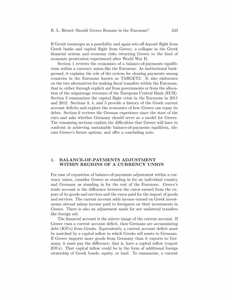
R. L. Hetzel: Should Greece Remain in the Eurozone? 243
If Grexit reemerges as a possibility and again sets o¤deposit �ight fromGreek banks and capital �ight from Greece, a collapse in the Greek�nancial system and economy risks returning Greece to the kind ofeconomic prostration experienced after World War II.
Section 1 reviews the economics of a balance-of-payments equilib-rium within a currency union like the Eurozone. As institutional back-ground, it explains the role of the system for clearing payments amongcountries in the Eurozone known as TARGET2. It also elaborateson the two alternatives for making �scal transfers within the Eurozone,that is, either through explicit aid from governments or from the alloca-tion of the seigniorage revenues of the European Central Bank (ECB).Section 2 summarizes the capital �ight crisis in the Eurozone in 2011and 2012. Sections 3, 4, and 5 provide a history of the Greek currentaccount de�cits and explore the economics of how Greece can repay itsdebts. Section 6 reviews the German experience since the start of theeuro and asks whether Germany should serve as a model for Greece.The remaining sections explain the di¢ culties that Greece will have toconfront in achieving sustainable balance-of-payments equilibria, dis-cuss Greece�s future options, and o¤er a concluding note.
1. BALANCE-OF-PAYMENTS ADJUSTMENTWITHIN REGIONS OF A CURRENCY UNION
For ease of exposition of balance-of-payments adjustment within a cur-rency union, consider Greece as standing in for an individual countryand Germany as standing in for the rest of the Eurozone. Greece�strade account is the di¤erence between the euros earned from the ex-port of its goods and services and the euros paid for the import of goodsand services. The current account adds income earned on Greek invest-ments abroad minus income paid to foreigners on their investments inGreece. There is also an adjustment made for net unilateral transferslike foreign aid.
The �nancial account is the mirror image of the current account. IfGreece runs a current account de�cit, then Germans are accumulatingdebt (IOUs) from Greeks. Equivalently, a current account de�cit mustbe matched by a capital in�ow in which Greeks sell assets to Germans.If Greece imports more goods from Germany than it exports to Ger-many, it must pay the di¤erence, that is, have a capital in�ow (exportIOUs). That capital in�ow could be in the form of additional foreignownership of Greek bonds, equity, or land. To summarize, a current

244 Federal Reserve Bank of Richmond Economic Quarterly
account de�cit implies an o¤setting capital in�ow and a current accountsurplus implies an o¤setting capital out�ow.3
Assume that Greece and Germany had their own currencies andthat the Greek drachma and the German mark �oated freely againsteach other. Assume also a sudden stop in in�ows of private capitalthat had been �nancing a Greek current account de�cit. In this event,the drachma would depreciate relative to the mark in order to main-tain balance-of-payments equilibrium. Greece�s terms of trade woulddepreciate in that its goods would become less expensive relative toGerman goods. However, with a currency union, settlement is in thesingle currency, the euro. The accounting identity between the currentand the capital account of course still holds. If, say, a Greek currentaccount de�cit exceeds the private capital in�ow from Germany, thenthe di¤erence is made up for by a transfer of bank reserves from Greeceto Germany. Bank reserves decline in Greece and increase in Germany.
In a world without monetary frictions, the associated decline inthe money stock in Greece would cause a decline in the Greek pricelevel (de�ation) while the increase in the money stock in Germanywould cause an increase in the German price level (in�ation). Thedepreciation in the Greek terms of trade arises from this change inrelative price levels. In reality, the required de�ation in Greece takestime. As a result, when capital in�ows precipitately become capitalout�ows and money contracts (�sudden stops�), the required suddenbalance between imports and exports occurs through recession thatrestricts the demand for imports.
In order to understand better the working of sudden stops in capitalin�ows in the context of the Eurozone, it is helpful to understand someinstitutional details. First, it is useful to note the way in which themembers of the Eurozone clear payments among themselves using theTARGET2 system.4 It is a payments clearing system that records net�ows of bank reserves among Eurozone member countries. Second, theECB allows banks to borrow for extended periods. As a result, whenthe banks in Greece lose reserves, they can replace them by borrowingfrom the ECB through their national central bank, the Bank of Greece.That is, the national central bank creates new reserves to replace thereserves lost to German banks.
3 The �nancial account records transactions for direct investment, portfolio invest-ment, and other investment, which includes bank deposits and reserves. The discussionignores the capital account, which is typically small. It records capital transfers such asdebt forgiveness.
4 TARGET2 is the abbreviation for the Trans-European Automated Real-time GrossSettlement Express Transfer system 2. It is the large-value cross-border payments andsettlement system for the Eurozone.
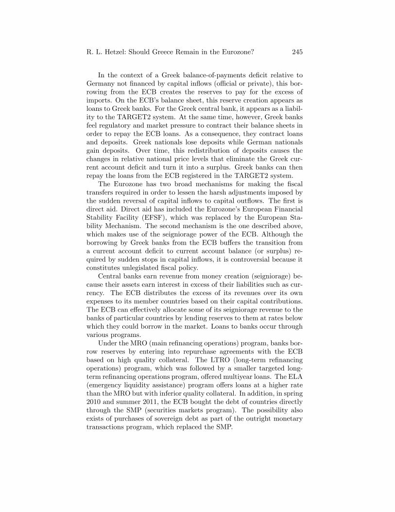
R. L. Hetzel: Should Greece Remain in the Eurozone? 245
In the context of a Greek balance-of-payments de�cit relative toGermany not �nanced by capital in�ows (o¢ cial or private), this bor-rowing from the ECB creates the reserves to pay for the excess ofimports. On the ECB�s balance sheet, this reserve creation appears asloans to Greek banks. For the Greek central bank, it appears as a liabil-ity to the TARGET2 system. At the same time, however, Greek banksfeel regulatory and market pressure to contract their balance sheets inorder to repay the ECB loans. As a consequence, they contract loansand deposits. Greek nationals lose deposits while German nationalsgain deposits. Over time, this redistribution of deposits causes thechanges in relative national price levels that eliminate the Greek cur-rent account de�cit and turn it into a surplus. Greek banks can thenrepay the loans from the ECB registered in the TARGET2 system.
The Eurozone has two broad mechanisms for making the �scaltransfers required in order to lessen the harsh adjustments imposed bythe sudden reversal of capital in�ows to capital out�ows. The �rst isdirect aid. Direct aid has included the Eurozone�s European FinancialStability Facility (EFSF), which was replaced by the European Sta-bility Mechanism. The second mechanism is the one described above,which makes use of the seigniorage power of the ECB. Although theborrowing by Greek banks from the ECB bu¤ers the transition froma current account de�cit to current account balance (or surplus) re-quired by sudden stops in capital in�ows, it is controversial because itconstitutes unlegislated �scal policy.
Central banks earn revenue from money creation (seigniorage) be-cause their assets earn interest in excess of their liabilities such as cur-rency. The ECB distributes the excess of its revenues over its ownexpenses to its member countries based on their capital contributions.The ECB can e¤ectively allocate some of its seigniorage revenue to thebanks of particular countries by lending reserves to them at rates belowwhich they could borrow in the market. Loans to banks occur throughvarious programs.
Under the MRO (main re�nancing operations) program, banks bor-row reserves by entering into repurchase agreements with the ECBbased on high quality collateral. The LTRO (long-term re�nancingoperations) program, which was followed by a smaller targeted long-term re�nancing operations program, o¤ered multiyear loans. The ELA(emergency liquidity assistance) program o¤ers loans at a higher ratethan the MRO but with inferior quality collateral. In addition, in spring2010 and summer 2011, the ECB bought the debt of countries directlythrough the SMP (securities markets program). The possibility alsoexists of purchases of sovereign debt as part of the outright monetarytransactions program, which replaced the SMP.
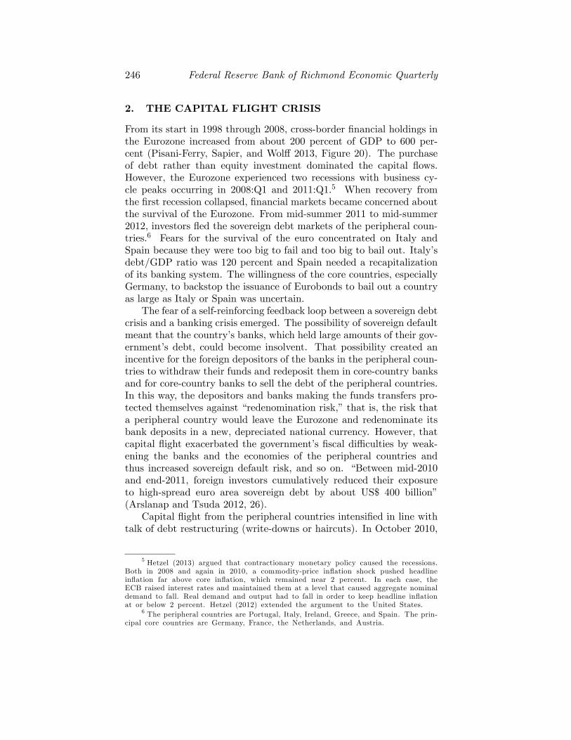
246 Federal Reserve Bank of Richmond Economic Quarterly
2. THE CAPITAL FLIGHT CRISIS
From its start in 1998 through 2008, cross-border �nancial holdings inthe Eurozone increased from about 200 percent of GDP to 600 per-cent (Pisani-Ferry, Sapier, and Wol¤ 2013, Figure 20). The purchaseof debt rather than equity investment dominated the capital �ows.However, the Eurozone experienced two recessions with business cy-cle peaks occurring in 2008:Q1 and 2011:Q1.5 When recovery fromthe �rst recession collapsed, �nancial markets became concerned aboutthe survival of the Eurozone. From mid-summer 2011 to mid-summer2012, investors �ed the sovereign debt markets of the peripheral coun-tries.6 Fears for the survival of the euro concentrated on Italy andSpain because they were too big to fail and too big to bail out. Italy�sdebt/GDP ratio was 120 percent and Spain needed a recapitalizationof its banking system. The willingness of the core countries, especiallyGermany, to backstop the issuance of Eurobonds to bail out a countryas large as Italy or Spain was uncertain.
The fear of a self-reinforcing feedback loop between a sovereign debtcrisis and a banking crisis emerged. The possibility of sovereign defaultmeant that the country�s banks, which held large amounts of their gov-ernment�s debt, could become insolvent. That possibility created anincentive for the foreign depositors of the banks in the peripheral coun-tries to withdraw their funds and redeposit them in core-country banksand for core-country banks to sell the debt of the peripheral countries.In this way, the depositors and banks making the funds transfers pro-tected themselves against �redenomination risk,�that is, the risk thata peripheral country would leave the Eurozone and redenominate itsbank deposits in a new, depreciated national currency. However, thatcapital �ight exacerbated the government�s �scal di¢ culties by weak-ening the banks and the economies of the peripheral countries andthus increased sovereign default risk, and so on. �Between mid-2010and end-2011, foreign investors cumulatively reduced their exposureto high-spread euro area sovereign debt by about US$ 400 billion�(Arslanap and Tsuda 2012, 26).
Capital �ight from the peripheral countries intensi�ed in line withtalk of debt restructuring (write-downs or haircuts). In October 2010,
5 Hetzel (2013) argued that contractionary monetary policy caused the recessions.Both in 2008 and again in 2010, a commodity-price in�ation shock pushed headlinein�ation far above core in�ation, which remained near 2 percent. In each case, theECB raised interest rates and maintained them at a level that caused aggregate nominaldemand to fall. Real demand and output had to fall in order to keep headline in�ationat or below 2 percent. Hetzel (2012) extended the argument to the United States.
6 The peripheral countries are Portugal, Italy, Ireland, Greece, and Spain. The prin-cipal core countries are Germany, France, the Netherlands, and Austria.

R. L. Hetzel: Should Greece Remain in the Eurozone? 247
in Deauville, France, German Chancellor Angela Merkel and FrenchPresident Nicolas Sarkozy agreed that in the future government debtsecurities would include collective action clauses, which would facilitaterestructuring. The principle of debt write-downs became known asprivate sector involvement (PSI). �[I]n July 2011, debt restructuringwas o¢ cially endorsed [by the European Union Council] as an optionfor Greece....But agreement on a deep PSI had to wait until October2011, and negotiations were only completed in February 2012�prior tothe Second Economic Adjustment Program announced in March 2012(Pisani-Ferry, Sapier, and Wol¤ 2013, 42, 68).7 By early 2012, holdersof Greek debt, chie�y French and German banks, had either sold orallowed the debt to run o¤. As a consequence, 80 percent of Greekdebt passed into the hands of foreign o¢ cial institutions (the EFSF,the ECB, and the International Monetary Fund [IMF]) with much ofthe remainder held by Greek banks (Slok 2015).
The decision not to require Eurozone banks to write o¤ their Greekdebt but rather to convert it into debt held by o¢ cial creditors was con-troversial in that it kept the Greek debt-to-GDP ratio at an extremelyhigh level. At the time, the Euro area ruled out debt restructuring.The required approval of Eurozone parliaments would have been un-likely (International Monetary Fund 2013b, 27). From 2001 to 2009,Greek government debt held externally by the private sector went fromabout e80 billion to about e225 billion. By 2012, it had declined toless than e50 billion. On the �ip side, between 2009 and 2012, Greekgovernment debt held by o¢ cial creditors went from zero to about e225billion (International Monetary Fund 2013b, 18).
Cecchetti, McCauley, and McGuire (2012) noted that the part of acurrent account de�cit not �nanced by private capital in�ows or o¢ cialaid would register in the form of a TARGET2 imbalance. (TARGET2imbalances in turn measure the key variable� bank borrowing from theECB.) They provided the following taxonomy of the capital-�ight cri-sis of the peripheral countries. From 2002 to mid-2007, private capitalin�ows completely �nanced current account de�cits. From mid-2007through 2009, private capital �ows �nanced three-�fths of their cur-rent account de�cits. From 2010 through 2011, as re�ected in TAR-GET2 imbalances, borrowing from the ECB by banks in the peripheralcountries �nanced all of current account de�cits. However, in 2012:Q1and 2012:Q2, the growth of TARGET2 imbalances far outpaced the
7 Gulati, Trebesch, and Zettlmeyer (2012, Abstract) put the aggregate haircut onprivately outstanding Greek debt at 55 percent�65 percent depending upon the valuationof the old bonds and estimated the debt relief received by Greece to be on the orderof 48 percent of GDP.

248 Federal Reserve Bank of Richmond Economic Quarterly
current account de�cits. As Cecchetti, McCauley, and McGuire noted,their growth corresponded to capital �ight, that is, the transfer of de-posits from the banks of peripheral countries to those of core countries,especially to German banks.8
Using current account and TARGET2 data, Vihriälä (2013)concluded:
Between April 2010 and August 2012, net private capital out�owstotaled 167bn [euros] in Greece, 118bn in Ireland and 99bn in Portugal.In terms of pre-crisis GDP, these �gures amount to about 75%, 62%and 59% respectively. Starting in summer 2011, private investorsstarted to leave also Italy and Spain, which between May 2011 andAugust 2012 recorded out�ows of 303bn (19% of pre-crisis GDP)and 364bn (35% of pre-crisis GDP)....Before the announcement [ECBPresident Mario Draghi�s pledge to do �whatever it takes�to preservethe monetary union] a larger and larger share of Greek, Irish, Italianand Spanish bonds had been o¤-loaded by foreign investors andacquired by domestic banks. . . .
The ECB contributed signi�cantly to the �scal transfers requiredto o¤set capital �ight from the peripheral countries of the Eurozone.That fact appears in the increase in the size of the ECB�s balance sheet.Measured relative to Eurozone GDP, in fall 2008, it went from about15 percent to 20 percent. In spring 2011, it began to increase again,reaching somewhat more than 30 percent by early 2013. The expansionin the ECB�s balance sheet appeared in the diminution of the impor-tance attached to its traditional means of supplying reserves to banksthrough the short-term auction of funds, the MROs. In their place,the ECB began supplying reserves through LTROs, which redirectedlending toward banks in the periphery.
3. GREEK BALANCE-OF-PAYMENTSADJUSTMENT
The underlying premise here is that the capital in�ows and currentaccount de�cit that accompanied Greek membership in the Eurozonein 2001 caused its real terms of trade to appreciate through an in�ationrate in excess of the Eurozone average. The capital �ight that began
8 In the case of Greece, over the period from mid-2011 to mid-2012, the increasein borrowing from the Bank of Greece exceeded the increase in TARGET2 liabilitiesby about e30 billion. The di¤erence re�ected the extent of an internal currency drain,that is, withdrawals of cash held under mattresses. However, if a Greek bank borrowsfrom the Bank of Greece in order to replace reserves lost due to a wire transfer bya depositor at a Greek bank to the account of a bank in Frankfurt, then TARGET2liabilities increase.
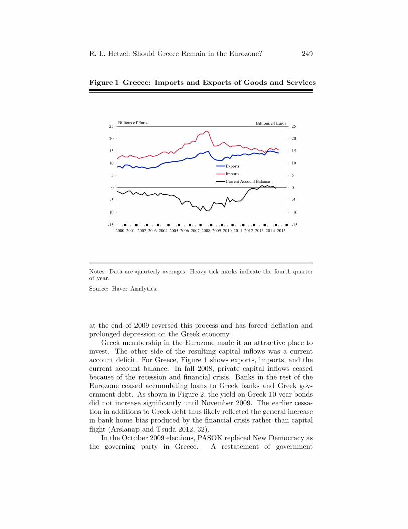
R. L. Hetzel: Should Greece Remain in the Eurozone? 249
Figure 1 Greece: Imports and Exports of Goods and Services
Notes: Data are quarterly averages. Heavy tick marks indicate the fourth quarterof year.
Source: Haver Analytics.
at the end of 2009 reversed this process and has forced de�ation andprolonged depression on the Greek economy.
Greek membership in the Eurozone made it an attractive place toinvest. The other side of the resulting capital in�ows was a currentaccount de�cit. For Greece, Figure 1 shows exports, imports, and thecurrent account balance. In fall 2008, private capital in�ows ceasedbecause of the recession and �nancial crisis. Banks in the rest of theEurozone ceased accumulating loans to Greek banks and Greek gov-ernment debt. As shown in Figure 2, the yield on Greek 10-year bondsdid not increase signi�cantly until November 2009. The earlier cessa-tion in additions to Greek debt thus likely re�ected the general increasein bank home bias produced by the �nancial crisis rather than capital�ight (Arslanap and Tsuda 2012, 32).
In the October 2009 elections, PASOK replaced New Democracy asthe governing party in Greece. A restatement of government

250 Federal Reserve Bank of Richmond Economic Quarterly
Figure 2 Yields on 10-Year Government Bonds
Notes: Heavy tick marks indicate December.
Source: ECB and Haver Analytics.
�nances revealed a large government de�cit, currently estimated at 9.5percent of GDP for 2008 (Federal Reserve Bank of St. Louis FREDdatabase). �Sentiment deteriorated further in November [2009] whenthe estimated 2009 �scal de�cit was revised from 13 1
2 to 1512 percent
of GDP, and in December there were general strikes and rioting in re-sponse to the labor reforms�(International Monetary Fund 2013b, 35).Concerns then arose over the sustainability of the Greek budget de�citand the solvency of Greek banks, which held considerable amounts ofGreek government debt. In 2010, foreign investors began selling Greekgovernment debt and the cessation of capital in�ows turned into out-right capital out�ows. In 2011, private capital �ight worsened as partof the general sovereign debt crisis a¤ecting the peripheral countries ofthe Eurozone.9
9 Eurozone banks� loans to Greece reached about e128 billion in 2008 and fell toabout e12 billion in September 2013 (Merler 2015).

R. L. Hetzel: Should Greece Remain in the Eurozone? 251
In March 2010, the European Commission, the ECB, and the IMFformed the Troika in order to coordinate lending to Greece based on�conditionality.�10 Starting with bilateral loans to Greece in April 2010from member countries of the Eurozone, the Eurozone has providedconsiderable direct aid to Greece. The Eurozone created the EFSF tocoordinate Eurozone government aid. Fear of a Greek exit from theEurozone grew starting in the last half of 2011 and reached its peakintensity in the �rst half of 2012.11 Considerable doubt existed as towhether Greece would implement the terms of the February 2012 Sec-ond Economic Adjustment Program, which had replaced the originaladjustment program of May 2010. The June 17, 2012, parliamentaryelections resulted in a coalition government formed by Prime Minis-ter Antonis Samaris, who made clear that Greece would accept theTroika adjustment program. In November 2012, the Greek Parliamentapproved the austerity package.
The ECB is the residual lender �nancing the Greek payments im-balance (current account de�cit plus net capital �ows) not covered bythe other Troika members. In the �rst instance, when Greeks importmore than they export or capital �ows out of the country, Greek bankslose reserves. They replace those reserves by borrowing from the ECBin one of the ways described above. From a negligible amount priorto mid-2008 to mid-2011, the share of Greek banks in total MRO andLTRO �nancing from the ECB rose to 20 percent (Pisani-Ferry, Sapier,and Wol¤ 2013, Figure 2). In summer 2011, Greek banks turned to theELA facility (Milligan 2012). ELA borrowing from the Bank of Greecerose to e120 billion by summer 2012 (Pisani-Ferry, Sapier, and Wol¤2013, Figure 3). By early 2012, the Bank of Greece funded about 30percent of the liabilities of Greek banks (European Central Bank 2015).
Figure 3 o¤ers insight into how Greece has �nanced its currentaccount de�cit and dealt with capital �ight. The cumulative currentaccount de�cit measures the amount of debt that Greece owes the restof the world as a consequence of past trade de�cits.12 That debt canbe held by private investors who voluntarily invest in Greece, by theECB in the form of lending to Greek banks and in the form of Greek
10 The European Commission acts on behalf of the member states whose govern-ments must approve the disbursement of funds from the EFSF.
11 �As 2011 progressed, a Greek euro exit became a serious possibility particularlyafter being discussed by Euro leaders at the Cannes summit in November 2011. Thegovernment then announced a referendum to test the views of the Greek people. Thiswas subsequently cancelled but the government resigned later that month and was re-placed by a technocratic government� (International Monetary Fund 2013b, 35).
12 It is roughly equal to the net international investment position, which includeschanges in asset valuations of assets held in Greece by foreigners and by Greeks abroad.

252 Federal Reserve Bank of Richmond Economic Quarterly
Figure 3 Greece: Sources of Financing the Current AccountDe�cit
Notes: Heavy tick marks indicate fourth quarter of year.
Source: EuroStat, Haver Analytics, and European Commission (April and August2014).
government debt held outright, and by foreign o¢ cial institutions (theIMF and Eurozone stabilization funds).13
As shown in Figure 1, Greece ran a current account de�cit from2000 through 2012 when the de�cit approached zero. As a result, inFigure 3, the blue line showing the cumulative current account declineduntil end 2012.14 The fact that TARGET2 liabilities (shown by the redline) were essentially zero until 2008 implies that private capital in�owslargely �nanced the current account de�cit until then.15 After 2008,Greek TARGET2 liabilities mounted. Greece then �nanced its current
13 The Wall Street Journal (2015b) gave the following breakdown (in billions of eu-ros) for early 2015: EFSF (131.0), Eurozone governments (52.9), private investors (34.1),ECB (26.9), IMF (21.1), and Treasury bill holders (14.8). The ECB �gure does not in-clude lending to Greek banks.
14 The line showing the cumulative current account de�cit starts at e �45 bil-lion, which is the cumulative current account de�cit run from 1980 through 1999(Eurostat/Haver).
15 Financial aid from the European Union for structural adjustment (not balanceof payments aid) was also signi�cant. As a percentage of Greek GDP, it averaged 2.5percent from 2000 through 2007 (Bitros, Batavia, and Nandakumar 2014, Table 1). As

R. L. Hetzel: Should Greece Remain in the Eurozone? 253
account de�cit through spending down its bank reserves, which Greekbanks replaced by borrowing from the ECB as indicated by the increasein TARGET2 liabilities. Starting in May 2010, Greece began to receiveregular disbursements from external, o¢ cial sources. In Figure 3, theblack line measuring this aid mounts to nearly e225 billion. In 2010,2011, and 2012, Greece �nanced its current account de�cit and o¤setreserve out�ows produced by capital �ight through the combined aidof the o¢ cial institutions and from ECB borrowing as registered by theincrease in TARGET2 liabilities. Thereafter and continuing through2014, as shown by the decline in TARGET2 liabilities, Greece usedo¢ cial aid to repay much of its ECB borrowing and some externallyheld private debt.
In January 2015, the uncertainty created by the replacement ofthe New Democracy government of Prime Minister Samaris with theSyriza government of Prime Minister Alexis Tsipras again producedcapital �ight and runs on banks. ELA borrowing by Greek banks rosewhile TARGET2 liabilities again increased (Figure 3). ECB funding ofGreek banks (MRO, LTRO, and ELA lending) peaked at about e135billion in summer 2012; fell to about e40 billion in late 2014; and thenrose again to somewhat above e100 billion in February 2015 (DeutscheBank 2015, 6). As of March 2015, Greek banks had liabilities of aboute550 billion.16
4. THE GREEK TRANSFER PROBLEM
The repayment of the euro-denominated debt owed by Greece to itsexternal creditors (the IMF, the ECB, the EFSF, and now chie�y hedgefunds) requires a transfer of resources to foreigners.17 That is, Greecemust run a balance of trade surplus. For that to happen, the Greekintra-Eurozone terms of trade must depreciate.18 There are two aspectsto the required terms of trade depreciation.
a percentage of GDP, the Greek current account de�cit averaged 6.7 percent from 2000to 2005. The ratio deteriorated to 14.2 percent in 2007�08.
16 From Bank of Greece, �aggregated balance sheet of MFIs.� The ECB limits theability of the four largest Greek banks to add to their net holdings of Greek Treasurybills. In doing so, it prevents the Greek government from �nancing de�cits by issuingTreasury bills to the banks, which then use them as collateral to borrow from the ELAfacility.
17 The term �transfer problem� came from a debate in the late 1920s between JohnMaynard Keynes and Bertil Ohlin over the feasibility of making the resource transfersimplied by the reparations imposed upon Germany after World War I.
18 In principle, the euro could depreciate relative to currencies like the dollar su¢ -ciently in order for Greece to run a balance of trade surplus (current account surplus)with the rest of the world large enough to o¤set a de�cit with Eurozone countries. Thatpossibility is unlikely and the analysis focuses exclusively on the Greek intra-Eurozoneterms of trade.
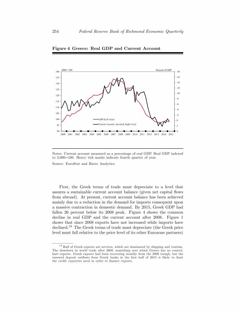
254 Federal Reserve Bank of Richmond Economic Quarterly
Figure 4 Greece: Real GDP and Current Account
Notes: Current account measured as a percentage of real GDP. Real GDP indexedto 2,000=100. Heavy tick marks indicate fourth quarter of year.
Source: EuroStat and Haver Analytics.
First, the Greek terms of trade must depreciate to a level thatassures a sustainable current account balance (given net capital �owsfrom abroad). At present, current account balance has been achievedmainly due to a reduction in the demand for imports consequent upona massive contraction in domestic demand. By 2015, Greek GDP hadfallen 26 percent below its 2008 peak. Figure 4 shows the commondecline in real GDP and the current account after 2008. Figure 1shows that since 2008 exports have not increased while imports havedeclined.19 The Greek terms of trade must depreciate (the Greek pricelevel must fall relative to the price level of its other Eurozone partners)
19 Half of Greek exports are services, which are dominated by shipping and tourism.The slowdown in world trade after 2008, something over which Greece has no control,hurt exports. Greek exports had been recovering steadily from the 2009 trough, but therenewed deposit out�ows from Greek banks in the �rst half of 2015 is likely to limitthe credit exporters need in order to �nance exports.

R. L. Hetzel: Should Greece Remain in the Eurozone? 255
in order to achieve current account balance (net of private capital �owsfrom abroad) at full employment.
Second, there must be a one-time adjustment (overshooting) in theterms of trade depreciation that generates the current account surplusrequired in order to pay o¤ the external debt.20 Greece�s Eurozonecreditors have lengthened considerably the maturity of the debt owedby Greece. Even with Greece�s present elevated debt-to-GDP ratio,Greece need only transfer about 2 percent of its GDP annually (Wol¤2015b). Equivalently, it need only run an annual current account sur-plus of that magnitude apart from net private capital �ows.21 Althoughthese numbers are not unusual for countries, they do add to the requiredterms-of-trade depreciation.
In a world in which price levels adjusted without friction, the Greekterms of trade would depreciate through a reduction in its domesticprice level. According to the classical price-specie mechanism of DavidHume, how would this occur?22 Consider the annual payment for anextended period of, say, e1 billion to external creditors. The Greekgovernment would �rst run a budget surplus of e1 billion, which wouldincrease its account with the Bank of Greece by that amount and re-duce the deposits of Greek nationals by the same amount. It wouldthen write a check, say, to the EFSF. When the EFSF cashes its checkdrawn on the Bank of Greece, the reserves of the Greek banking sys-tem decline. When the EFSF pays down its debt, the deposits of itsbondholders increase. Because its bondholders are almost exclusivelynon-Greek nationals, the reserves end up outside of Greece.
Assuming that Greek banks cannot borrow from the ECB in orderto make up the loss, they sell assets or call in loans in order to obtainreserves. As a result, Greek nationals experience a reduction in theireuro deposits. (That reduction would not occur if the Greek govern-ment had used its budget surplus in order to make domestic purchases.)In order to bring their money holdings back to the desired level, Greeknationals reduce their expenditures. Greece needs to run an annualcurrent account surplus (excess of exports over imports) of e1 billionin order to import the euros required to replenish the depleted cashbalances of its nationals. Adjustment occurs when the Greek price
20 In 2008, Greece�s debt-to-GDP ratio was 117 percent. It rose to 171 percent in2012 and then increased slightly to 175 percent in 2014 (Federal Reserve Bank of St.Louis FRED database).
21 �Greece bene�ts from an average loan maturity of over 30 years. The countrypays neither interest nor redemption on the overwhelming part of its EFSF loans until2023� (Credit Suisse 2015).
22 David Hume ([1742] 1955) described the equilibrating mechanism for the balanceof payments known as the price-specie-�ow mechanism in a gold standard.

256 Federal Reserve Bank of Richmond Economic Quarterly
Figure 5 Germany-Greece: Real Final Sales to DomesticPurchasers
Notes: Real �nal sales to domestic purchasers expressed as four-quarter percent-age change. Real �nal sales to domestic purchasers is real GDP minus the changein inventories minus net exports. Heavy tick marks indicate fourth quarter of year.
Source: Haver Analytics.
level has fallen su¢ ciently (the Greek terms of trade have depreciatedsu¢ ciently) in order to generate the required current account surplus.
The problem is that the price level does not adjust in a frictionlessmanner. There is the inherent disruption to production in forcing anunanticipated price-level reduction, which disturbs all relative prices.Those relative prices convey the information required to allocate re-sources. As shown in Figure 5, Greece and Germany both experiencedrecession with cycle troughs in 2009. Both recovered, but the recov-ery in Greece aborted in 2010 with the return to monetary contractionshown in Figure 6, related to the capital �ight discussed above. Figure6 shows for Greece the relationship between growth in money (M1) andin nominal GDP.23 Broadly, the two series move together.
Figure 6 raises the issue of simultaneity. Because the ECB operateswith an interest rate instrument, nominal GDP could determine the
23 In the absence of data on currency, M1 is sight deposits at Greek banks.

R. L. Hetzel: Should Greece Remain in the Eurozone? 257
Figure 6 Greece: M1 and Nominal GDP
Notes: Quarterly percentage changes in M1 and nominal GDP. Heavy tick marksindicate fourth quarter of year.
Source: Hellenic Statistical Authority (ELSTAT)/Haver Analytics.
behavior of M1 within the Eurozone. Because Greece is only a smallpart of Eurozone GDP, Greek citizens can control their net exports inorder to adjust their money holdings to nominal GDP. Figure 7 showsreal money holdings for Greece� the ratio of M1 and M2 to nominalGDP or the inverse of velocity. What evidence is there that the relativestability in the M1 series re�ects adjustment of nominal GDP (euroexpenditure) to M1 holdings? Consider both series in Figure 7, whichshow real money demand expressed as the inverse of velocity, that is,the ratio of money to nominal GDP.
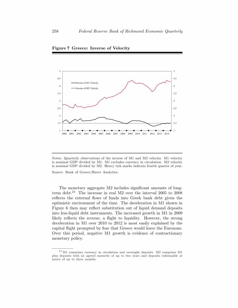
258 Federal Reserve Bank of Richmond Economic Quarterly
Figure 7 Greece: Inverse of Velocity
Notes: Quarterly observations of the inverse of M1 and M2 velocity. M1 velocityis nominal GDP divided by M1. M1 excludes currency in circulation. M2 velocityis nominal GDP divided by M2. Heavy tick marks indicate fourth quarter of year.
Source: Bank of Greece/Haver Analytics.
The monetary aggregate M2 includes signi�cant amounts of long-term debt.24 The increase in real M2 over the interval 2005 to 2008re�ects the external �ows of funds into Greek bank debt given theoptimistic environment of the time. The deceleration in M1 shown inFigure 6 then may re�ect substitution out of liquid demand depositsinto less-liquid debt instruments. The increased growth in M1 in 2009likely re�ects the reverse, a �ight to liquidity. However, the strongdeceleration in M1 over 2010 to 2012 is most easily explained by thecapital �ight prompted by fear that Greece would leave the Eurozone.Over this period, negative M1 growth is evidence of contractionarymonetary policy.
24 M1 comprises currency in circulation and overnight deposits. M2 comprises M1plus deposits with an agreed maturity of up to two years and deposits redeemable atnotice of up to three months.
R. L. Hetzel: Should Greece Remain in the Eurozone? 259
It seems likely that the transmission of the monetary shock to thereal economy occurred to a signi�cant extent through �nancial fric-tions. The reduction in bank reserves associated with the sudden stopin capital in�ows caused banks to restrict credit.25 As a result, house-holds and �rms had to restrict expenditures. Exporters could not getthe trade credit they require in order to export. Also, when capital�ows in and �nances a current account de�cit, the price of assets likeland rises. The fall in asset prices that accompanies a reversal of cap-ital in�ows disrupts �nancial intermediation when those assets serveas collateral. The essential monetary phenomenon remains, however,that a depreciation of Greece�s intra-Eurozone terms of trade requiresde�ation.
The debt-de�ation trap that Irving Fisher talked about in the 1930sapplies to Greece. Fisher pointed out that de�ation not anticipatedat the time the parties entered into the debt contract leaves debtorswith unexpectedly high debt burdens. The de�ation that Greece mustendure in order to generate the current account surpluses requiredto pay o¤ its external debt raises the real burden imposed by euro-denominated debt. In a world of frictionless renegotiation of debtcontracts, some combination of personal bankruptcy and restructur-ing would occur and economic activity would continue. However, inany country and especially in Greece with a poorly functioning judicialsystem, debt default is disruptive. Households and �rms do not receivethe credit they need in order to deal with disruptions to their cash �owand to make productive investments.
In a country like Greece where markets are highly cartelized, de-�ation is all the more disruptive and occurs only with recession andhigh levels of unemployment. The recession increases debt in a num-ber of ways. First, it can permanently lower the productive capabilityof the economy.26 Second, as output falls, tax revenue falls and thegovernment de�cit increases. Third, if households and �rms default ontheir loans from banks, banks need recapitalization, further increasing
25 The reserves of Greek banks rose after August 2007 in line with other Eurozonebanks. The interbank market for reserves shrank as banks became concerned aboutlending to other banks whose portfolios could include U.S. subprime securities. TheECB replaced the market through full allotment of MRO lending that increased bankreserves to a level that limited the need for interbank borrowing. The reserves heldby Greek banks fell sharply after July 2012 when ECB president Mario Draghi saidthat the ECB would do �whatever it takes� in order to prevent capital �ight from theperipheral countries from breaking up the Eurozone.
26 �The trauma of recession has been so harsh as to force people and companies,particularly skilled people and good, pro�table companies, to leave Greece and set upoperation elsewhere� (Congdon 2013, 5).

260 Federal Reserve Bank of Richmond Economic Quarterly
the government de�cit.27 In order to render tolerable the su¤ering ofthe Greek people and prevent complete economic collapse, the �insti-tutions� (the Troika) extend additional loans to Greece. In order toachieve repayment, the addition to the debt burden then requires evenmore de�ation. In 2005, Greece�s debt-to-GDP ratio was 98.6 percent,which rose modestly to 105.4 percent in 2008. However, during thedepression it increased sharply to an estimated 174.9 percent in 2014.
As a matter of arithmetic, the debt-to-GDP ratio (Dt) equals theproduct of the prior period�s ratio (Dt�1) times the ratio of one plusthe interest rate on the debt to one plus the growth rate of GDP minusthe primary budget balance relative to GDP (PB):
Dt = Dt�1
�1 + it1 + yt
�� PB: (1)
Debt sustainability is a requirement of an IMF assistance program.That is, given its program, the IMF must forecast a declining value ofDin (1). As part of the two adjustment programs, it did so based in parton a forecast of positive future nominal GDP (y) growth. Speci�cally,it forecast a return to positive real GDP growth in 2012 combined withcontinued positive in�ation, apart from price stability in 2011 (Interna-tional Monetary Fund 2013b, 13). In fact, the growth rate of nominalGDP became negative in 2008:Q2 and remained negative through 2013.Instead of turning positive in 2012, real GDP growth was near �6 per-cent in 2012. It seems likely that additional aid to Greece will requirethe politically di¢ cult decision by the Eurozone countries to lend morewhile also forgiving existing debt, perhaps through lengthening the ma-turity of repayment.
5. WHY DEFLATION IS NOT OVER
O¢ cial IMF forecasts have regularly fallen short in their estimation ofthe time that would be required for Greece to emerge from recessionand exit its bailout programs. One possible reason for the unwarrantedoptimism was the limited experience of the IMF in dealing with crisesin a monetary union. Pisani-Ferry, Sapier, and Wol¤ (2013, 10�1)noted that the majority of past IMF programs �were accompanied bya sharp currency depreciation.�Among countries with �xed exchange
27 �The payment culture has been weakened, including through repeated morato-ria on auctioning foreclosed assets. And the insolvency framework has been unable todeal with either the rehabilitation of viable entities or the liquidation of non-viable en-tities....[R]esources remain trapped in unproductive or ine¢ cient activities....Greece hasone of the highest levels of NPLs [nonperforming loans] globally� (International Mone-tary Fund 2014, 15).

R. L. Hetzel: Should Greece Remain in the Eurozone? 261
rates that received IMF bailouts, almost all had capital controls. Incontrast, until July 2015, Greece had �irrevocably �xed exchange ratesand a regime of unfettered capital �ows.�That is, the terms of tradeadjustment had to occur through de�ation rather than depreciation ofthe currency.
Using measures of the real e¤ective exchange rate (REER) for coun-tries in the Asian and Latin American crises, Pisani-Ferry, Sapier, andWol¤ (2013, 10�1) calculated the currency depreciation that occurredduring the crises.28 For the Latin American countries, the depreciationamounted to about 40 percent. For the Asian countries, the initial de-preciation was about 40 percent but then settled down at 30 percent.Comparison with the Asian and Latin American experiences suggeststhat Greece could need an even larger depreciation in its terms of trade.These countries went into the crisis with current account de�cits notfar from 5 percent. Greece went into the crisis with a current accountde�cit of 15 percent.29
A number of factors apart from those mentioned in the previoussection exacerbate the internal de�ation required by Greece. First, af-ter the crisis, the Greek terms of trade appreciated. Figure 8 showsGerman and Greek in�ation. Greek in�ation actually increased afterthe crisis. The increase in excise taxes and the value-added tax requiredby the terms of the 2010 bailout pushed up prices with the e¤ect of in-creasing the ultimate required de�ation. Moreover, as shown in Figure8, the disin�ation in the Eurozone, which appears in declining Germanin�ation, implies that in order to depreciate its terms of trade Greecemust de�ate.30
Second, the adjustment is more severe if the country starts withsigni�cant external debt. Payment of the interest and principal onthe debt then necessitates running current account surpluses beyondsimply eliminating the de�cit. Toward the end of 2013, the ratio ofexternal debt to GDP was about 100 percent in Greece (Goldman Sachs2013, 3). Third, the smaller the tradeable goods sector relative to thenontradeable goods sector, the more di¢ cult it is to expand exports. In
28 The REER is calculated as a trade weighted-average of the exchange rates ofthe country with its trading partners adjusted by the consumer price indices (CPIs)of the country and its trading partners. The Asian crisis countries, with crisis datesin parentheses, were Indonesia (1997), Korea (1997), Thailand (1997), and the Philip-pines (1998). The Latin American countries were Brazil (1998), Argentina (2000), andUruguay (2002).
29 In the May 2010 assistance program for Greece, the Troika estimated the �needof a real exchange-rate depreciation...of the order of 20�30 percent� (Pisani-Ferry, Sapier,and Wol¤ 2013, 67).
30 Since 2009, core CPI in�ation for the Eurozone has fallen short of 2 percent. InMay 2015, year-over-year core CPI Eurozone in�ation was .9 percent.

262 Federal Reserve Bank of Richmond Economic Quarterly
Figure 8 Germany-Greece: In ation
Notes: In�ation is the harmonized CPI. Monthly observations of 12-month per-centage changes. Heavy tick marks indicate December.
Source: Haver Analytics.
Greece, the tradeable goods and services sector is just above 30 percent.In Ireland, in contrast, it is near 50 percent (Goldman Sachs 2013,6). Although by the end of 2012, Greece had come close to currentaccount balance, much of the improvement came from the e¤ects ofsevere recession in depressing imports (Figure 4). That fact suggeststhat the de�ation required in order to achieve a sustained surplus in thecurrent account has only just begun. Because imports will increase asthe economy recovers, it seems likely that Greece must de�ate furtherin order to achieve an internal Eurozone terms of trade consistent withfull employment.
Between 2000:Q1 and 2014:Q3, the Greek terms of trade appreci-ated relative to Germany�s terms of trade in that the Greek CPI rose45 percent and the German CPI rose 25 percent (Figure 9). If the ap-preciation in the Greek terms of trade that occurred in the �rst decadeof the Eurozone was due solely to a capital in�ow that will not return,Greek de�ation will have to undo the prior in�ation di¤erence betweenit and its Eurozone partners. Since 2012, with some Greek de�ation,

R. L. Hetzel: Should Greece Remain in the Eurozone? 263
Figure 9 Germany-Greece: In ation Divergence
Notes: Consumer prices indexed to January 2000=100. Heavy tick marks indicatefourth quarter of year.
Source: EuroStat and Haver Analytics.
the Greek terms of trade have depreciated but only a little. Moreover,because other peripheral countries like Spain and Ireland have becomemore competitive, Greece may have to undergo an even more prolongedde�ation in order to restore external trade balance.
Figure 10 tells a similar story in terms of the divergence in unitlabor costs. The Greek/German di¤erence widened through 2009 butnarrowed subsequently.31 The comparison with Germany rather thanwith other Eurozone countries does understate the progress Greece hasmade. Calculation of the real e¤ective exchange rate while showingonly moderate depreciation based on the CPI shows signi�cant im-provement based on unit labor costs (International Monetary Fund2013b, 37). (An o¤setting factor is that reducing the Greek unemploy-ment rate of 26 percent and a youth unemployment rate of 49 percent
31 The May 2010 IMF program had an objective of eliminating a �20�30 percentcompetitiveness gap...through wage adjustment and productivity gains� (InternationalMonetary Fund 2013b, 1). Without recourse to a depreciation of its currency, Greecehad to achieve the required reduction in unit labor costs through some combination ofdomestic de�ation and productivity increases.

264 Federal Reserve Bank of Richmond Economic Quarterly
Figure 10 Germany-Greece: Nominal Unit Labor Costs
Notes: Quarterly data. Heavy tick marks indicate fourth quarter of year.
Source: EuroStat and Haver Analytics.
will draw additional workers into the labor force with lower productiv-ity and will likely increase unit labor costs.) As the Eurozone recoverygains momentum, the reduction in its unit labor costs should bene�tGreece�s exports. The key issue then is whether dysfunction in theGreek banking system will limit exports by restricting the access ofGreek exporters to credit.32
In order to free the resources required for an excess of exports overimports at full employment, Greece must achieve an internal as wellas an external terms-of-trade depreciation. First, in order to channeldomestic production into exports, Greek unit labor costs will likelyhave to decline further. Without increases in productivity, real wagesmust fall through a greater decline in nominal wages than in prices.
32 In Ireland, Spain, and Portugal, the return to current account balance by 2015has come in signi�cant part from an increase in exports (Wol¤ 2015a). The contrastwith Greece likely re�ects in part the better functioning of these countries bankingsystems.
R. L. Hetzel: Should Greece Remain in the Eurozone? 265
Second, in order to draw resources into the export sector, the priceof nontradeable goods must decline relative to the price of tradeablegoods. According to the International Monetary Fund (2013b, 37),Greece has not progressed in this respect: �Despite reform attempts,professions like pharmacology and law, as well as the transport andenergy sectors, remained closed to new entrants. Continuing protectioncaused prices of nontradeables to remain elevated relative to the pricesof tradeables. . . .�
6. IS GERMANY A GOOD MODEL FOR GREECE?
When the Eurozone began operation, Germany was in some respectsin the position in which Greece �nds itself in 2015. Germany enteredthe Eurozone in 1999 with an exchange rate that overvalued its goodsand services. As a consequence, after its entry into the Eurozone in1999, it had to experience low in�ation and high unemployment. Priorto its entry, in the context of instability in the European exchange ratemechanism, capital in�ows into Germany had appreciated the Germanmark, traditionally the strongest currency in Europe. The other reasonfor the overvaluation of the mark at the creation of the Eurozone wentback to German reuni�cation.
As shown in Figure 11, Germany normally runs a current accountsurplus. That is, it is a net capital exporter. After the fall of the BerlinWall and reuni�cation of East and West Germany, the requirementsof infrastructure investment in East Germany meant that Germanyneeded for a while to change from a capital exporter into a capitalimporter (Hetzel 2002). In order to provide the additional resourcesneeded in Germany, Germans had to buy more from foreigners, who inturn had to buy less from Germans. This reversal required that pricesin Germany had to rise more than the prices of its trading partners.Germany�s terms of trade had to appreciate.
Germany�s current account de�cit became moderately negative from1990 through 2001. Thereafter, it rose steadily and stabilized at around7 percent of GDP. Figure 12 breaks the current account de�cit into ex-ports and imports. Germany�s success as an exporter appears in theincrease in its exports as a percentage of GDP from around 27 percentin the 1980s to more than 45 percent at present. One reason for thatsuccess was that German labor unions were willing to hold down wagegrowth in order to limit the movement of manufacturing jobs to theformerly communist Eastern European countries.33 As a result, unit
33 �Germany established its own new lower norm of zero nominal unit labor costin�ation resulting from a consensus between the trade unions, workers� representatives
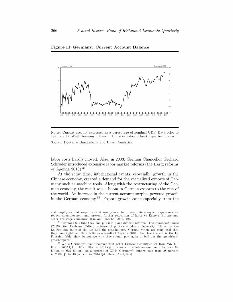
266 Federal Reserve Bank of Richmond Economic Quarterly
Figure 11 Germany: Current Account Balance
Notes: Current account expressed as a percentage of nominal GDP. Data prior to1991 are for West Germany. Heavy tick marks indicate fourth quarter of year.
Source: Deutsche Bundesbank and Haver Analytics.
labor costs hardly moved. Also, in 2003, German Chancellor GerhardSchröder introduced extensive labor market reforms (the Hartz reformsor Agenda 2010).34
At the same time, international events, especially, growth in theChinese economy, created a demand for the specialized exports of Ger-many such as machine tools. Along with the restructuring of the Ger-man economy, the result was a boom in German exports to the rest ofthe world. An increase in the current account surplus powered growthin the German economy.35 Export growth came especially from the
and employers that wage restraint was pivotal to preserve Germany�s competitiveness,reduce unemployment and prevent further relocation of labor to Eastern Europe andother low-wage countries� (Lin and Treichel 2012, 12).
34 Germans felt that they had put into place di¢ cult reforms. The Financial Times(2013) cited Professor Falter, professor of politics at Mainz University: �It is like theLa Fontaine fable of the ant and the grasshopper. German voters are convinced thatthey have tightened their belts as a result of Agenda 2010....And like the ant in the LaFontaine fable, they do not see why they should pay again to bail out the spendthriftgrasshoppers.�
35 While Germany�s trade balance with other Eurozone countries fell from e37 bil-lion in 2007:Q4 to e18 billion in 2014:Q4, it rose with non-Eurozone countries from e4billion to e27 billion. As a percent of GDP, Germany�s exports rose from 28 percentin 2000:Q1 to 48 percent in 2014:Q4 (Haver Analytics).
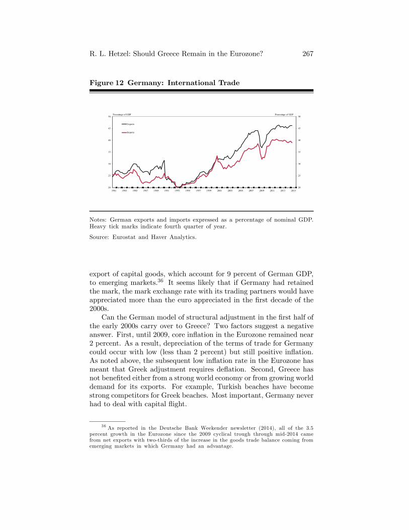
R. L. Hetzel: Should Greece Remain in the Eurozone? 267
Figure 12 Germany: International Trade
Notes: German exports and imports expressed as a percentage of nominal GDP.Heavy tick marks indicate fourth quarter of year.
Source: Eurostat and Haver Analytics.
export of capital goods, which account for 9 percent of German GDP,to emerging markets.36 It seems likely that if Germany had retainedthe mark, the mark exchange rate with its trading partners would haveappreciated more than the euro appreciated in the �rst decade of the2000s.
Can the German model of structural adjustment in the �rst half ofthe early 2000s carry over to Greece? Two factors suggest a negativeanswer. First, until 2009, core in�ation in the Eurozone remained near2 percent. As a result, depreciation of the terms of trade for Germanycould occur with low (less than 2 percent) but still positive in�ation.As noted above, the subsequent low in�ation rate in the Eurozone hasmeant that Greek adjustment requires de�ation. Second, Greece hasnot bene�ted either from a strong world economy or from growing worlddemand for its exports. For example, Turkish beaches have becomestrong competitors for Greek beaches. Most important, Germany neverhad to deal with capital �ight.
36 As reported in the Deutsche Bank Weekender newsletter (2014), all of the 3.5percent growth in the Eurozone since the 2009 cyclical trough through mid-2014 camefrom net exports with two-thirds of the increase in the goods trade balance coming fromemerging markets in which Germany had an advantage.
268 Federal Reserve Bank of Richmond Economic Quarterly
7. IS ABANDONING THE EURO A PRACTICABLESOLUTION FOR GREECE?
The assumption here is that the euro is so thoroughly embedded inGreek society that the reintroduction of the drachma combined witha �oating exchange rate would not eliminate the need for continuedGreek de�ation. The reason is that the Greeks would continue to usethe euro rather than the drachma for money.37
Money serves three functions. It is a medium of exchange, a store ofvalue, and a unit of account. Reintroduction of the drachma even withits required use for the payment of taxes and in government transac-tions would not necessarily entail its replacement of the euro for thesefunctions. The reintroduction of the drachma would most surely beaccompanied by the expectation that it would depreciate� an expec-tation likely to be self-ful�lling. Greeks would continue to rely on theeuro for money.
In principle, the Greek government could reintroduce the drachmawith the commitment to maintain internal price stability. With thepassage of years, perseverance could make the commitment credible,and Greek citizens would again use the drachma for all three functionsof money. In the interval, however, the euro would continue as themedium of exchange for high-value transactions, as a store of value,and as the unit of account. The depreciation of the terms of traderequired for external stability would require the same de�ation in theeuro prices that Greeks would continue to assign to their goods as iscurrently required with the euro as the national currency.
The conclusion is that Greece will need to continue with de�ation.However, the uncertain pace and amount of the de�ation means thatit cannot be anticipated in a way that is built into forward-lookingprice setting and into euro contracts. Consequently, it will continueto depress economic activity. A relaxation of austerity, which mightlessen the distress caused by the depression, is unlikely. Greece hashad to impose �scal austerity in order to run a primary �scal sur-plus (a surplus before interest payments on debt). It has had nochoice but to run a primary surplus. Otherwise, investors would ques-tion whether the government would ever raise the revenue to repay itsdebt. At 1.2 percent of GDP in 2014, the primary balance (excluding
37 From 1991 until 2002, Argentina operated a currency board. That is, it con-verted dollars and pesos at a one-for-one ratio while allowing the change in pesos topass directly through to the peso monetary base. Because the pesos continued to circu-late as currency, for Argentina, which su¤ered de�ation under its currency board, theoption existed of abandoning the currency board and depreciating the peso. Unfortu-nately for Greece, the fact that unlike the peso the drachma disappeared makes the caseof Argentina inapplicable.

R. L. Hetzel: Should Greece Remain in the Eurozone? 269
one-time adjustments) o¤ers a minimal margin for increasing govern-ment expenditure (Darvas 2015, Annex). Structural reform can lessenthe need for depreciation in the Greek terms of trade and thus for de-�ation. The following section o¤ers some comments on why structuralreform is so di¢ cult.
8. THE DIFFICULTY OF STRUCTURAL REFORM
George Bitros (2013, 26), professor emeritus at Athens University ofEconomics and Business, argued that �the public budget became thespoils of politicians, tightly organized minorities and interlocking groupsof business interests�and that the movement away from a free-marketeconomy to an economy organized around monopolies and governmentregulation occurred �mainly because of the sharp partisan competitionthat emerged in the political arena� after the ousting of the militarygovernment in 1974. The impression left by Bitros is that, given theweakness of Greek institutions, politicians found it costly to form thecoalitions required to hold power. Given the weakness of the statein raising tax revenues, political parties thus found it expedient toencourage the formation of cartels. These cartels, which are pro-tected from competition, receive rents (monopoly returns) in returnfor government-enforced restrictions on entry. E¤ectively, a monopolycan impose and collect a tax that does not appear on the government�sbooks.
Hayashi, Li, and Wang (2015, 1) summarized the stylized factssurrounding the innovation that leads to new industries. �As new in-dustries evolve from birth to maturity, it is typically observed thatprice falls, output rises, and �rm numbers initially rise and later fall.�Researchers term the decline in �rm numbers �shakeout.�The lessonis that the innovation spurred by competition requires free entry andfree exit. The highly regulated Greek economy discourages both.
Slok (2012) reported the World Bank ranking of countries accordingto ease of doing business. In 2013, Greece ranked 78 overall but rankedeven lower in key categories. For example, in the category �startinga business,�which measures factors such as days required in order toobtain a license, Greece ranked 146. In registering property, it ranked150, and in enforcing contracts it ranked 87. As a condition for Troikaassistance, Greece passed laws liberalizing entry into markets and pro-fessions but then delayed their implementation (International MonetaryFund 2013b, 18). In Greece, there are more than 500 regulated pro-fessions accounting for about one-third of employment (InternationalMonetary Fund 2013a, 15). Similarly, Greece has moved only slowlyto eliminate employment protection laws. The International Monetary
270 Federal Reserve Bank of Richmond Economic Quarterly
Fund (2014, 23) noted with respect to the law that limits collective dis-missals, �[N]o such dismissal has been approved for thirty years. . . .�Heavy government regulation along with the arbitrary application oflaws encourages corruption (Cambanis 2014).
Still, a balanced view must recognize that over the years 2010 to2014, Greece did make signi�cant progress in reforming its governmentand economy. Among the countries receiving bailout support from thecountries of the Eurozone, Greece�s �scal restructuring was the mostrigorous. Zsolt Darvas (2015, Table 1) calculated the structural pri-mary balance for Greece excluding one-o¤ receipts and payments suchas the cost of recapitalizing the banking system. Thus, his �gures notonly account for one-time adjustments but also for cyclical in�uences,which increase the de�cit, and for payments on debt. For Greece, thestructural primary balance went from -10.0 percent of GDP in 2009 to6.1 percent of GDP in 2014.
A key demand of Greece�s creditors has been for pension reform.Greece has made signi�cant cuts in its pension payments both presentand promised (Gupta 2012). Because Greece has not had a signi�cantprivate pension system, pensioners depend upon government pensionsand many now live in or near poverty. At the same time, Greek demo-graphics render the government pension system insolvent over the longrun. Greece�s spending on pensions as a percent of GDP at 17.5 percentin 2012 is the highest in Europe. Moreover, only 36 percent of Greeksaged 55�64 work compared to 63 percent in Germany (The Economist2015). Long-term demographics are unfavorable. �More than one in�ve Greeks is older than 65, making it the world�s �fth oldest nation.Just 14 percent is under 15, a smaller share of youngsters entering thelabor force than all but nine other countries�(Goldenberg 2015).
9. WHERE TO GO FROM HERE
Unfortunately, dialogue between Greece and its creditors about theway forward is di¢ cult because of the divergence of views about thecauses of the Greek depression. A �creditor�view often associated withGermany is that �scal indiscipline in Greece led to an unsustainablelevel of debt. The collapse of the stimulus to demand provided by thislevel of debt led to the depression. A related �German�view is that thelong-term viability of the Eurozone depends upon adherence to rules.Rules enforcing �scal discipline prevent the Eurozone from becominga transfer union in which the more �scally responsible members bailout the less �scally responsible members. From this perspective, it isessential that Greece run a primary surplus su¢ cient to repay the loansfrom other Eurozone members. The debate is intensi�ed by criticism

R. L. Hetzel: Should Greece Remain in the Eurozone? 271
that Greece broke the rules of the Maastricht Treaty requiring �scaldiscipline. For example, Jose Manuel Barroso, the former president ofthe European Commission, argued (European Commission, 2013):38
We have a Stability and Growth Pact. We have rules...so these un-employed people in Greece should be told that the authorities of theircountry did not respect the Treaties that they have signed....[T]hebiggest lesson of the crisis...is that growth based on debt is notsustainable.
More succinctly, The Wall Street Journal (2013) wrote:
[C]reating a rigid �Europe of Rules�is exactly the German-led strat-egy for managing the crisis. Berlin�s aim is to perfect the monetaryunion by ensuring countries adhere to rules designed to prevent futurecrises by addressing what are seen as the causes of the current one:government overspending and excessive risk-taking by banks.
A contrasting view common in Greece is that its recession is due tothe �scal consolidation required by its o¢ cial creditors. Based on aninterview, Hansen (2015, 36, 38, 52) o¤ered insights into the views offormer Greek Finance Minister Yanis Varoufakis:
Varoufakis has staked his academic integrity on a particular economicand moral critique of the crisis....Greece, he said, would no longer sim-ply acquiesce to the austerity doctrine of the European Commission,the European Central Bank and the I.M.F....Varoufakis...wanted toshow the Europeans how to save Europe itself....Varoufakis traces hispolitical consciousness to his childhood in �the junta era�....�I amnot going to fold on pensions� or on restoring collective bargainingrights.
Moreover, many members of Syriza are committed socialists whoare opposed to free market reforms and privatization on principle. Theydo not see a free-market economy as allocating resources to their mostproductive use but rather as a license for the powerful to exploit theweak. Upon taking power, the Syriza government indicated a desireto undo the labor market reforms agreed to under the previous twoadjustment programs such as lowering the minimum wage, weaken-ing collective bargaining requirements, and limiting the prohibition ofcollective dismissals. No doubt for this reason, the text of the Euro
38 Critics of the German policy of austerity have pointed out that Germany brokethe rules of the Maastricht Treaty when it ran a de�cit of 4 percent of GDP in 2004with a debt-to-GDP ratio of almost 65 percent. However, Germany never had to worryabout capital �ight.

272 Federal Reserve Bank of Richmond Economic Quarterly
Figure 13 Greece: Total Deposits and Banknotes inCirculation
Notes: Heavy tick marks indicate December. Data are from Bank of Greece.Deposits are from Aggregated Balance Sheet of Monetary Financial Institutions.Banknotes in circulation are from Bank of Greece Financial Statement. The seriesis �Banknotes in circulation,�which is based on a formula, plus �Net liabilities re-lated to the allocation of euro banknotes within the Eurosystem,� which is basedon the additional issuance of banknotes.
Source: Bank of Greece and Bloomberg.
Summit statement on Greece of July 13, 2015, required Greece to com-ply with detailed reforms in its product and labor markets.
The stando¤ between Greece and its creditors came to a head onJuly 12, 2015. The imminent collapse of the Greek banking systemforced Greece into accepting the demands of its creditors. From Janu-ary 2010 through June 2012, deposits �owed out of Greek banks. FromJuly 2012 through November 2014, their deposits stabilized. Start-ing in December 2014, however, with the political uncertainty createdby Syriza coming to power, signi�cant out�ows of deposits resumed(Figure 13).
In this situation, the ECB became the key player. The Greek gov-ernment had avoided the imposition of capital controls only because

R. L. Hetzel: Should Greece Remain in the Eurozone? 273
the ECB had regularly raised the cap on ELA lending by the Bank ofGreece in order to �nance the out�ows of deposits from Greek banks.Doing so required the ECB Governing Council every two weeks to cer-tify the solvency of the four large Greek banks that the ECB supervises.However, in the absence of an agreement between Greece and its cred-itors, the ECB was in a di¢ cult situation. As the single regulator forthe large banks of the Eurozone, it had to worry about its credibilityfor certifying the health of banks. Moreover, in the event of a de-fault by the Greek government on its debt, it would have trouble usingGreek government debt to collateralize its lending to Greek banks. Asa central bank, the ECB is constrained by the central bank principleof lending only on good collateral.
At the end of June, Greek Prime Minister Alexis Tsipras inter-rupted negotiations with Greece�s creditors in order to hold a referen-dum on July 5 on their proposal. Greece�s EFSF assistance programexpired at the end of June and it failed to make a payment owed to theIMF. Out�ows of deposits from Greek banks then surged. When theECB declined to raise the ELA limit further, the Greek governmentimposed capital controls on banks. Greek depositors could only with-draw a limited amount of cash each day from banks and they couldnot transfer funds out of the country. Lacking the ability to transferfunds abroad, importers could not import. Exporters also su¤ered fromnot being able to import raw materials. The possibility that the ECBwould close Greek banks by ending ELA lending broke the impasse andstarted negotiations for a third adjustment program on terms set by theIMF and the European Commission representing the �nance ministersof the Eurozone.
10. A REASON FOR HOPE
It is not realistic to believe that Greece can leave the Eurozone. Eventhough Greece had its own printing presses before the introduction ofthe euro, the paper for printing the bills has to be ordered from abroad.It takes time to print money and distribute it among banks. In the timerequired to plan for the reintroduction of the drachma, depositors inGreek banks will have �ed. More fundamentally, money is a publicgood in the sense that its value comes from its universal acceptance.Only over a long period of �scal discipline could the Greek governmentpersuade its public to hold drachmas instead of euros as a store ofvalue.
The reality then is that Greece will likely have to continue de�a-tion for many years. In the near term, the increase in the value addedtax to a uniform 23 percent is an exogenous cost-push shock that will

274 Federal Reserve Bank of Richmond Economic Quarterly
Figure 14 Euro Area: GDP and Real M1 Growth Rate
Notes: Quarterly observations of four-quarter percentage changes in real M1. RealM1 lagged by four quarters. Real M1 is M1 divided by the CPI. Heavy tick marksindicate fourth quarter of year.
Source: M1 data from 1996 to 2012 are from the Bundesbank and M1 data from2012 to 2015 are from Haver Analytics.
exacerbate in�ation and further depress the Greek economy. How-ever, Greece can mitigate the need for de�ation through policies thatencourage voluntary capital in�ows. Remaining in the Eurozone willlimit the need for terms of trade depreciation by encouraging externalinvestment. A national commitment to deregulate markets in order toallow free entry and exit would also promote investment from abroad.In addition, free-market reforms would lessen the need for terms-of-trade depreciation through de�ation by creating a more competitiveexport sector.
There are reasons for optimism about the Eurozone economy. TheECB�s policy of quantitative easing will encourage continued recoveryand, if sustained, return in�ation to the 2 percent target. As shownin Figure 14, which plots real GDP and real M1 lagged four quarters,strong money growth presages a vigorous economic recovery (Irelandand Oracic 2015). A strong Eurozone recovery will encourage the de-mand for Greek exports and lessen the need for de�ation. Moreover,

R. L. Hetzel: Should Greece Remain in the Eurozone? 275
Spain has reformed its labor markets to a signi�cant degree and Irelandhas retained an open economy. Both are experiencing strong exportgrowth and strong economic recoveries. It is possible that their exam-ple will encourage a similar national consensus for reform in Greece.
Figure 13 shows Greek bank deposits and banknotes in circulation.It o¤ers a sensitive barometer of con�dence in Greece and its economy.The fact that deposits declined from 2010 to mid-2012 and then onlyslowly recovered indicates the length of time required in order to rebuildtrust in the banking system. Now that Greece has imposed capitalcontrols, depositors will be quick to withdraw deposits at any sign of�nancial stress. Reopening a recapitalized Greek banking system withgrowth in deposits and in lending will be a key measure of whetherGreece can again restore growth. For that to happen, the ECB willhave to commit to maintaining liquidity for Greek banks and Greecewill have to commit to structural reform.
In signi�cant ways, Greece was dealt a bad hand. Its problemswould have very likely been manageable without the double-dip reces-sion in the Eurozone (Hetzel 2013). However, it has also played poorlythe hand it was dealt. In the 1990s in the run up to Greece�s admissioninto the Eurozone, Greece engaged in a national conversation aboutthe need for �scal discipline and the structural reform required in or-der to become a viable member of the Eurozone. Once admitted to theEurozone, however, it backed away from these commitments. Now, aspart of renewed negotiations over reform combined with continued aidand debt relief, Greece must revive this conversation and decide whereits future lies.
REFERENCES
Arslanap, Serkan, and Takahiro Tsuda. 2012. �Tracking GlobalDemand for Advanced Economy Sovereign Debt.�InternationalMonetary Fund Working Paper WP/12/284 (December).
Bitros, George C. 2013. �From Riches to Rags or What Went Wrongin Greece.�Available at http://ssrn.com/abstract=2196347(December 31).

276 Federal Reserve Bank of Richmond Economic Quarterly
Bitros, George C., Bala Batavia, and Parameswar Nandakumar. 2014.�Economic Crisis in the European Periphery: An Assessment ofEMU Membership and Home Policy E¤ects Based on the GreekExperience.�Munich Personal RePEc Archive Paper 60596(December).
Cambanis, Thanassis. 2014. �Why Can�t Greece Shake Its CorruptionProblem?�Boston Globe, 22 August.
Cecchetti, Stephen G., Robert N. McCauley, and Patrick M.McGuire. 2012. �Interpreting TARGET2 Balances.�Bank forInternational Settlements Working Paper 393 (December).
Congdon, Tim. 2013. �An Update on the Greek Situation.�International Monetary Research Limited, 26 April.
Credit Suisse. 2015. �European Economics.�1 July.
Darvas, Zsolt. 2015. �Should Other Eurozone Programme CountriesWorry about a Reduced Greek Primary Surplus Target?�Bruegel,25 February.
Deutsche Bank. 2014. �db140weekender.�17 October.
Deutsche Bank. 2015. �Focus Europe: Time to Act.�Research EuropeEconomics, 20 March.
The Economist. 2015. �Greece and its creditors: Starting to list.�4April.
European Central Bank. 2015. Statistical Data Warehouse, 7 April.
European Commission. 2013. �Austerity and Growth Debate: WhatPresident Barroso Actually said at the Brussels Think TankDialogue.�Memo (April 23).
Federal Reserve Bank of St. Louis. Federal Reserve Economic Data(FRED). Available at https://research.stlouisfed.org/fred2/.
Financial Times. 2013. �Decade-old Reforms still Divide SocialDemocrats.�8 March, 2.
Goldenberg, Liz. 2015. �Greek Debt Woes Won�t End Even with Dealdue to Aging Population.�Bloomberg, 15 June.
Goldman Sachs. 2013. European Economics Analyst. Issue No. 13/03,17 January.
Gulati, Mitu, Christoph Trebesch, and Jeromin Zettlmeyer. 2012.�The Greek Debt Exchange: An Autopsy.�Manuscript(September 11).
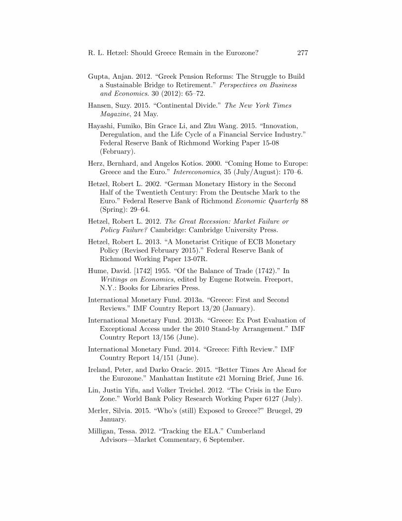
R. L. Hetzel: Should Greece Remain in the Eurozone? 277
Gupta, Anjan. 2012. �Greek Pension Reforms: The Struggle to Builda Sustainable Bridge to Retirement.�Perspectives on Businessand Economics. 30 (2012): 65�72.
Hansen, Suzy. 2015. �Continental Divide.�The New York TimesMagazine, 24 May.
Hayashi, Fumiko, Bin Grace Li, and Zhu Wang. 2015. �Innovation,Deregulation, and the Life Cycle of a Financial Service Industry.�Federal Reserve Bank of Richmond Working Paper 15-08(February).
Herz, Bernhard, and Angelos Kotios. 2000. �Coming Home to Europe:Greece and the Euro.�Intereconomics, 35 (July/August): 170�6.
Hetzel, Robert L. 2002. �German Monetary History in the SecondHalf of the Twentieth Century: From the Deutsche Mark to theEuro.�Federal Reserve Bank of Richmond Economic Quarterly 88(Spring): 29�64.
Hetzel, Robert L. 2012. The Great Recession: Market Failure orPolicy Failure? Cambridge: Cambridge University Press.
Hetzel, Robert L. 2013. �A Monetarist Critique of ECB MonetaryPolicy (Revised February 2015).�Federal Reserve Bank ofRichmond Working Paper 13-07R.
Hume, David. [1742] 1955. �Of the Balance of Trade (1742).�InWritings on Economics, edited by Eugene Rotwein. Freeport,N.Y.: Books for Libraries Press.
International Monetary Fund. 2013a. �Greece: First and SecondReviews.�IMF Country Report 13/20 (January).
International Monetary Fund. 2013b. �Greece: Ex Post Evaluation ofExceptional Access under the 2010 Stand-by Arrangement.�IMFCountry Report 13/156 (June).
International Monetary Fund. 2014. �Greece: Fifth Review.�IMFCountry Report 14/151 (June).
Ireland, Peter, and Darko Oracic. 2015. �Better Times Are Ahead forthe Eurozone.�Manhattan Institute e21 Morning Brief, June 16.
Lin, Justin Yifu, and Volker Treichel. 2012. �The Crisis in the EuroZone.�World Bank Policy Research Working Paper 6127 (July).
Merler, Silvia. 2015. �Who�s (still) Exposed to Greece?�Bruegel, 29January.
Milligan, Tessa. 2012. �Tracking the ELA.�CumberlandAdvisors� Market Commentary, 6 September.
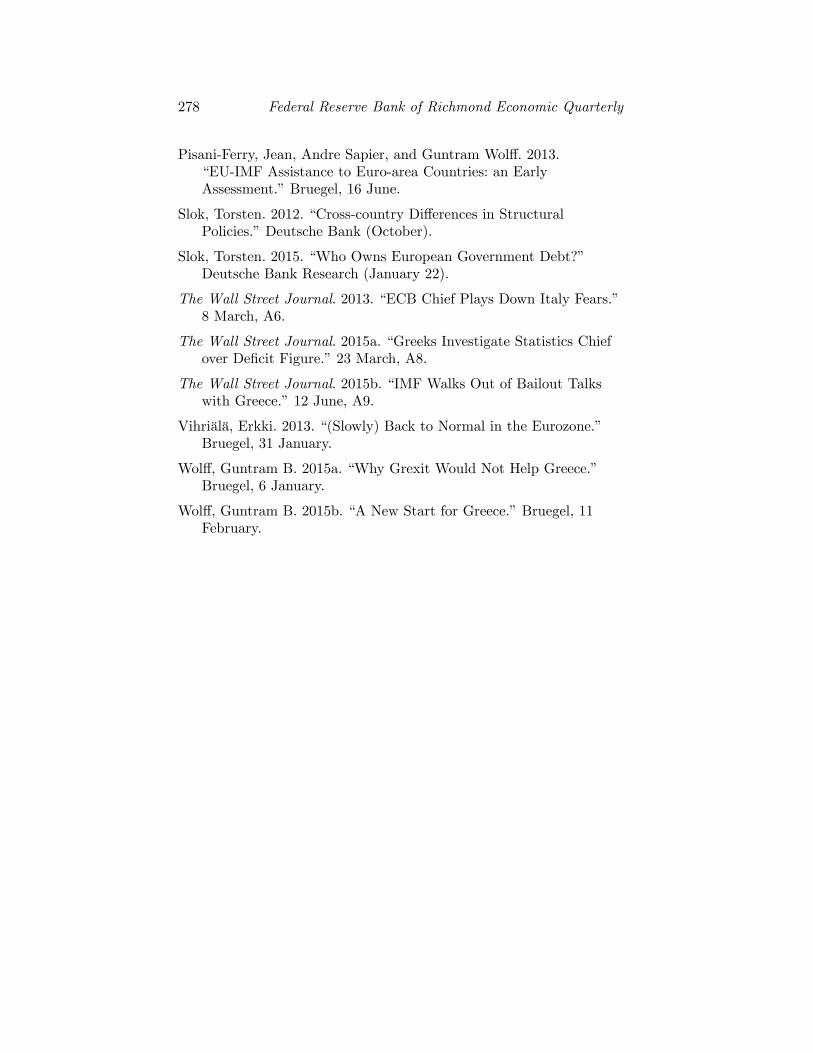
278 Federal Reserve Bank of Richmond Economic Quarterly
Pisani-Ferry, Jean, Andre Sapier, and Guntram Wol¤. 2013.�EU-IMF Assistance to Euro-area Countries: an EarlyAssessment.�Bruegel, 16 June.
Slok, Torsten. 2012. �Cross-country Di¤erences in StructuralPolicies.�Deutsche Bank (October).
Slok, Torsten. 2015. �Who Owns European Government Debt?�Deutsche Bank Research (January 22).
The Wall Street Journal. 2013. �ECB Chief Plays Down Italy Fears.�8 March, A6.
The Wall Street Journal. 2015a. �Greeks Investigate Statistics Chiefover De�cit Figure.�23 March, A8.
The Wall Street Journal. 2015b. �IMF Walks Out of Bailout Talkswith Greece.�12 June, A9.
Vihriälä, Erkki. 2013. �(Slowly) Back to Normal in the Eurozone.�Bruegel, 31 January.
Wol¤, Guntram B. 2015a. �Why Grexit Would Not Help Greece.�Bruegel, 6 January.
Wol¤, Guntram B. 2015b. �A New Start for Greece.�Bruegel, 11February.