Bioresource Technology 183 (2015) 163–174

Contents lists available at ScienceDirect

Bioresource Technology

journal homepage: www.elsevier .com/locate /bior tech

Reverse engineering of biochar

http://dx.doi.org/10.1016/j.biortech.2015.02.0430960-8524/� 2015 Elsevier Ltd. All rights reserved.

⇑ Corresponding author at: Inst. of Environmental Engineering, ETH Zürich,Zürich 8093, CH.

E-mail address: morales@ifu.baug.ethz.ch (V.L. Morales).

Verónica L. Morales a,⇑, Francisco J. Pérez-Reche b, Simona M. Hapca a, Kelly L. Hanley c,Johannes Lehmann c, Wei Zhang d

a SIMBIOS Centre, Abertay University, Dundee DD1 1HG, UKb Institute for Complex Systems and Mathematical Biology, SUPA, Department of Physics, University of Aberdeen, Old Aberdeen AB24 3UE, UKc Department of Crop and Soil Sciences, Cornell University, Ithaca, NY 1453, USAd Department of Plant, Soil and Microbial Sciences, Environmental Science and Policy Program, Michigan State University, East Lansing, MI 48824, USA

h i g h l i g h t s

� Starting biomass and peak pyrolysistemperature jointly affect biocharproperties.� 19 different physico-chemical

properties of biochar were properlymodeled by GLM.� Models reveal complex relationships

between biochar properties andpredictors.� Ubiquitous non-Gaussian and non-

linear attributes were accounted forin GLMs.� Proposed correlation networks,

models and web-tool can be used toengineer biochar.

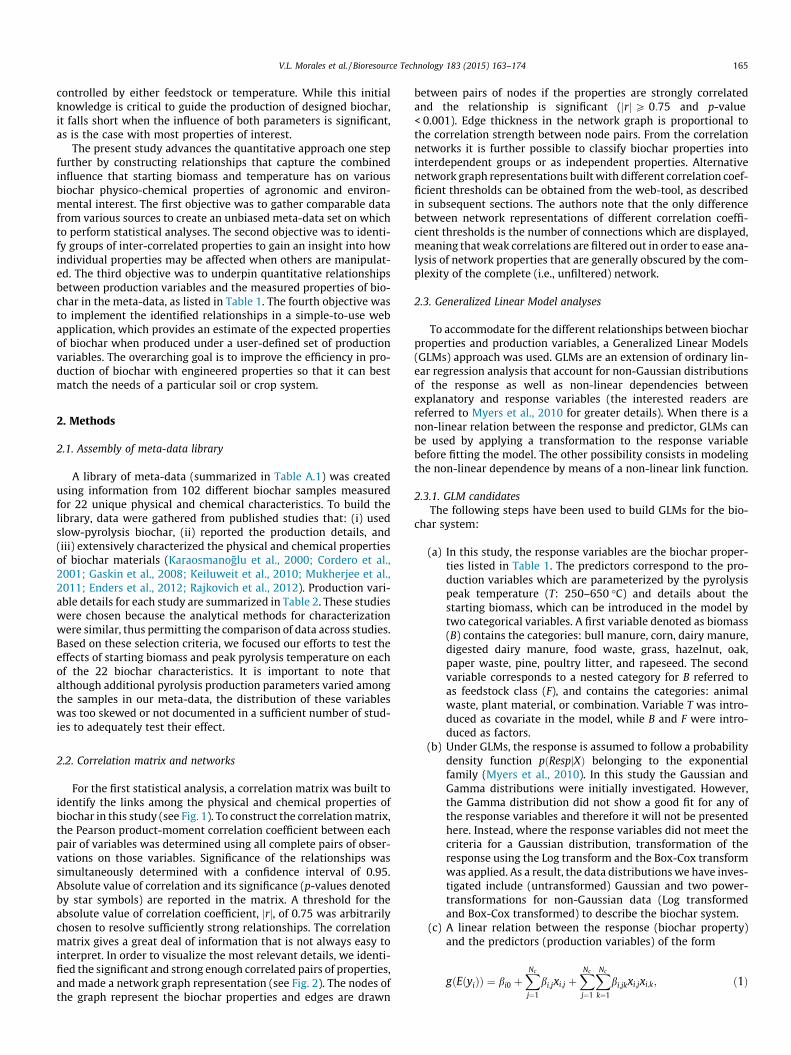
g r a p h i c a l a b s t r a c t

a r t i c l e i n f o

Article history:Received 24 December 2014Received in revised form 9 February 2015Accepted 10 February 2015Available online 18 February 2015

Keywords:Physico-chemical propertiesSlow-pyrolysisCorrelation networksGeneralized Linear ModelsWeb-tool

a b s t r a c t

This study underpins quantitative relationships that account for the combined effects that starting bio-mass and peak pyrolysis temperature have on physico-chemical properties of biochar. Meta-data wasassembled from published data of diverse biochar samples (n = 102) to (i) obtain networks of intercorre-lated properties and (ii) derive models that predict biochar properties. Assembled correlation networksprovide a qualitative overview of the combinations of biochar properties likely to occur in a sample. Gen-eralized Linear Models are constructed to account for situations of varying complexity, including: depen-dence of biochar properties on single or multiple predictor variables, where dependence on multiplevariables can have additive and/or interactive effects; non-linear relation between the response and pre-dictors; and non-Gaussian data distributions. The web-tool Biochar Engineering implements the derivedmodels to maximize their utility and distribution. Provided examples illustrate the practical use of thenetworks, models and web-tool to engineer biochars with prescribed properties desirable for hypo-thetical scenarios.

� 2015 Elsevier Ltd. All rights reserved.

1. Introduction

Biochar, the product of biomass thermochemical conversion inan oxygen depleted environment, has gained increasing recogni-tion as a modernized version of an ancient Amerindian soil man-agement practice, with at times wide-ranging agronomic and

Table 1Benefits from specific biochar properties.

Biochar property Agronomic and environmental benefits

BulkD [Mg m�3] Low bulk density biochar can reduce the densityof compacted soils, thereby improving rootpenetration (Atkinson et al., 2010; Ennis et al.,2011; Novak et al., 2013), water drainage andaeration (Joseph et al., 2009; Laird et al., 2010).The latter may mitigate green house gas emis-sions (Karhu et al., 2011).

SSA(N2), SSA(CO2)[m2 g�1]

High nanopore and micropore specific surfacearea, respectively, may increase the sorptiveaffinity of organic compounds to biochars(Cornelissen et al., 2005; Beesley et al., 2011), andimprove water holding capacity (Karhu et al.,2011).

Yield [%] Yield reflects the quantity of biochar materialproduced from the pyrolysis process.

EC [mS m�1] Electrical conductivity indicates the quantity ofsalt contained in the biochar. High EC canstabilize soil structure (Joseph et al., 2009;Hossain et al., 2011).

CEC [Av (mmolc kg�1)] Increased cation exchange capacity can improvethe soil’s ability to hold and exchange cations(Chapman, 1965; Glaser et al., 2002).

pHw [�] Soil solution pH directly affects soil surfacecharge, which determines the type ofexchangeable nutrients and mineral ions itattracts (Mukherjee et al., 2011). Additionally, thebuffering capacity of biochar can neutralize acidicsoils, redude aluminum toxicity and change thesoil microbial community structure (Abe, 1988;Lehmann et al., 2011).

Ash [%] Ash may improve the sorption capacity of biocharfor organic compounds and metals (Cao et al.,2011).

MatVol [%] Volatile matter affects biochar longevity in soil(Lehmann et al., 2011; Enders et al., 2012).Residual volatiles can also impact organic sub-stance sorption by blocking pores and changingsurface chemical interactions (Sander andPignatello, 2005; Zhu et al., 2005; Novak et al.,2013).

C [mg g�1] Total carbon in organic matter benefits the soil.N [mg g�1] Total nitrogen in the biochar supplies a

macronutrient, but its availability is limited.Biochar may strongly sorb ammonia and act as anitrogen-rich soil amendment (Spokas et al.,2012b).

C:N [�] Carbon to nitrogen ratio influences the rate ofdecomposition of organic matter and release ofsoil nitrogen (Novak et al., 2009).

FixedC [%] Fixed carbon is non-labile and therefore is aproperty attributed to biochar stability(Keiluweit et al., 2010; Enders et al., 2012;Rajkovich et al., 2012).

P, S [Total (mg kg�1)] Macronutrients provided by biochar, which canimprove soil fertility.

Ca, K, Mg, Na, Fe, Mn, Zn[Total (mg kg�1)]

Micronutrients provided by biochar, which canimprove soil fertility.

Notes: BulkD = bulk density, SSA = specific surface area, EC = electrical conduc-tivity, CEC = cation exchange capacity, MatVol = volatile matter, FixedC = fixedcarbon.

164 V.L. Morales et al. / Bioresource Technology 183 (2015) 163–174

environmental gains (Lehmann et al., 2003; Atkinson et al., 2010;Novak et al., 2013). Some of the most commonly acclaimed bene-fits of biochar application to soils include: increased long-term Cstorage in soils (Atkinson et al., 2010; Joseph et al., 2010; Crossand Sohi, 2011; Ennis et al., 2011; Karhu et al., 2011; Novaket al., 2013), restored soil fertility (Glaser et al., 2002; Lehmannet al., 2003; Gaskin et al., 2008; Novak et al., 2009; Atkinsonet al., 2010; Laird et al., 2010; Beesley et al., 2011; Lehmannet al., 2011; Enders et al., 2012; Spokas et al., 2012b; Novaket al., 2013), improved soil physical properties (Novak et al.,2009; Joseph et al., 2010; Ennis et al., 2011; Karhu et al., 2011;Lehmann et al., 2011; Novak et al., 2013), boosted crop yield andnutrition (Novak et al., 2009; Major et al., 2010; Lehmann et al.,2011; Rajkovich et al., 2012; Spokas et al., 2012a; Novak et al.,2013), enhanced retention of environmental contaminants(Cornelissen et al., 2005; Loganathan et al., 2009; Cao and Harris,2010; Beesley et al., 2011), and reduced N-emission and leaching(Spokas et al., 2012b; Novak et al., 2013). Examples of the specificbiochar properties responsible for these benefits are summarizedin Table 1.

Biochar quality can be highly variable, and its performance asan amendment – whether beneficial or detrimental – is oftenfound to depend heavily on its intrinsic properties and the par-ticular soil it is added to (Lehmann et al., 2003; Novak et al.,2009; Atkinson et al., 2010; Major et al., 2010; Lehmann et al.,2011; Spokas et al., 2012a). As has been previously concluded, bio-char application to soil is not a ‘‘one size fits all’’ paradigm (Spokaset al., 2012a; Novak et al., 2013). Consequently, detailed knowl-edge of the biochar properties and the specific soil deficiencies tobe remediated is critical to maximize the possible benefits andminimize undesired effects of its use as a soil amendment. Whilesoil deficiencies must be identified on a site-by-site basis, it is con-ceivable that biochar properties can be engineered through themanipulation of pyrolysis production parameters and proper selec-tion of parent biomass type (Zhao et al., 2013). The capacity to pro-duce biochars with consistent and predictable properties will, first,enable efficient matching of biochars to soils, and second, facilitatethe deployment of this soil management strategy at large and com-mercial scales. Although the properties and effects of biochar sam-ples produced from a variety of methods and starting biomasseshave been intensively studied, as yet, the analytical techniquesfor characterization and effect quantification are not standardized.This creates a challenge when comparing biochar properties andeffects across studies. At the same time, making such comparisonsis imperative to gain a comprehensive understanding of alterablebiochar properties.

The prevailing hypothesis in the literature is that the selectionof peak pyrolysis temperature and parent biomass – as two keyproduction variables – fundamentally affects resulting biocharproperties. Identification of relationships between production vari-ables and biochar properties has been pursued by many investiga-tors, but has been limited to the small number of samplesproduced and analyzed for each study (e.g., Karaosmanoglu et al.,2000; Zhu et al., 2005; Gaskin et al., 2008; Nguyen and Lehmann,2009; Cao and Harris, 2010; Joseph et al., 2010; Keiluweit et al.,2010; Cao et al., 2011; Cross and Sohi, 2011; Hossain et al., 2011;Mukherjee et al., 2011; Enders et al., 2012; Rajkovich et al.,2012; Zhao et al., 2013), with few reports combining measure-ments from more than one source (Cordero et al., 2001; Glaseret al., 2002; Atkinson et al., 2010; Ennis et al., 2011; Spokaset al., 2012a). The knowledge gained from the above studies doesnot provide a quantitative understanding of the relationshipsbetween production variables and biochar properties. The short-comings responsible for such lack of systematic insight include:(i) reported trends that are primarily qualitative with respect tothe independent effect of parent biomass or temperature (e.g.,

decrease in labile carbon with increasing pyrolysis temperaturefor selected samples (Cross and Sohi, 2011)), (ii) trends that areoften in conflict with similar samples of other studies (e.g., positiveeffect (Rajkovich et al., 2012) vs. negligible effect (Nguyen andLehmann, 2009) of temperature on pH for oak biochar), and (iii)correlations that are not convincing (e.g., correlation r = 0.5between volatile matter content and microporous surface area(Mukherjee et al., 2011)). A recent study by Zhao et al., 2013reports, for the first time, a quantitative evaluation of the indi-vidual influence of feedstock source and production temperatureon various biochar properties. The authors classified a variety ofphysical and chemical biochar properties as predominantly

V.L. Morales et al. / Bioresource Technology 183 (2015) 163–174 165

controlled by either feedstock or temperature. While this initialknowledge is critical to guide the production of designed biochar,it falls short when the influence of both parameters is significant,as is the case with most properties of interest.

The present study advances the quantitative approach one stepfurther by constructing relationships that capture the combinedinfluence that starting biomass and temperature has on variousbiochar physico-chemical properties of agronomic and environ-mental interest. The first objective was to gather comparable datafrom various sources to create an unbiased meta-data set on whichto perform statistical analyses. The second objective was to identi-fy groups of inter-correlated properties to gain an insight into howindividual properties may be affected when others are manipulat-ed. The third objective was to underpin quantitative relationshipsbetween production variables and the measured properties of bio-char in the meta-data, as listed in Table 1. The fourth objective wasto implement the identified relationships in a simple-to-use webapplication, which provides an estimate of the expected propertiesof biochar when produced under a user-defined set of productionvariables. The overarching goal is to improve the efficiency in pro-duction of biochar with engineered properties so that it can bestmatch the needs of a particular soil or crop system.

2. Methods

2.1. Assembly of meta-data library

A library of meta-data (summarized in Table A.1) was createdusing information from 102 different biochar samples measuredfor 22 unique physical and chemical characteristics. To build thelibrary, data were gathered from published studies that: (i) usedslow-pyrolysis biochar, (ii) reported the production details, and(iii) extensively characterized the physical and chemical propertiesof biochar materials (Karaosmanoglu et al., 2000; Cordero et al.,2001; Gaskin et al., 2008; Keiluweit et al., 2010; Mukherjee et al.,2011; Enders et al., 2012; Rajkovich et al., 2012). Production vari-able details for each study are summarized in Table 2. These studieswere chosen because the analytical methods for characterizationwere similar, thus permitting the comparison of data across studies.Based on these selection criteria, we focused our efforts to test theeffects of starting biomass and peak pyrolysis temperature on eachof the 22 biochar characteristics. It is important to note thatalthough additional pyrolysis production parameters varied amongthe samples in our meta-data, the distribution of these variableswas too skewed or not documented in a sufficient number of stud-ies to adequately test their effect.

2.2. Correlation matrix and networks

For the first statistical analysis, a correlation matrix was built toidentify the links among the physical and chemical properties ofbiochar in this study (see Fig. 1). To construct the correlation matrix,the Pearson product-moment correlation coefficient between eachpair of variables was determined using all complete pairs of obser-vations on those variables. Significance of the relationships wassimultaneously determined with a confidence interval of 0.95.Absolute value of correlation and its significance (p-values denotedby star symbols) are reported in the matrix. A threshold for theabsolute value of correlation coefficient, jrj, of 0.75 was arbitrarilychosen to resolve sufficiently strong relationships. The correlationmatrix gives a great deal of information that is not always easy tointerpret. In order to visualize the most relevant details, we identi-fied the significant and strong enough correlated pairs of properties,and made a network graph representation (see Fig. 2). The nodes ofthe graph represent the biochar properties and edges are drawn

between pairs of nodes if the properties are strongly correlatedand the relationship is significant (jrjP 0:75 and p-value< 0.001). Edge thickness in the network graph is proportional tothe correlation strength between node pairs. From the correlationnetworks it is further possible to classify biochar properties intointerdependent groups or as independent properties. Alternativenetwork graph representations built with different correlation coef-ficient thresholds can be obtained from the web-tool, as describedin subsequent sections. The authors note that the only differencebetween network representations of different correlation coeffi-cient thresholds is the number of connections which are displayed,meaning that weak correlations are filtered out in order to ease ana-lysis of network properties that are generally obscured by the com-plexity of the complete (i.e., unfiltered) network.

2.3. Generalized Linear Model analyses

To accommodate for the different relationships between biocharproperties and production variables, a Generalized Linear Models(GLMs) approach was used. GLMs are an extension of ordinary lin-ear regression analysis that account for non-Gaussian distributionsof the response as well as non-linear dependencies betweenexplanatory and response variables (the interested readers arereferred to Myers et al., 2010 for greater details). When there is anon-linear relation between the response and predictor, GLMs canbe used by applying a transformation to the response variablebefore fitting the model. The other possibility consists in modelingthe non-linear dependence by means of a non-linear link function.

2.3.1. GLM candidatesThe following steps have been used to build GLMs for the bio-

char system:

(a) In this study, the response variables are the biochar proper-ties listed in Table 1. The predictors correspond to the pro-duction variables which are parameterized by the pyrolysispeak temperature (T: 250–650 �C) and details about thestarting biomass, which can be introduced in the model bytwo categorical variables. A first variable denoted as biomass(B) contains the categories: bull manure, corn, dairy manure,digested dairy manure, food waste, grass, hazelnut, oak,paper waste, pine, poultry litter, and rapeseed. The secondvariable corresponds to a nested category for B referred toas feedstock class (F), and contains the categories: animalwaste, plant material, or combination. Variable T was intro-duced as covariate in the model, while B and F were intro-duced as factors.

(b) Under GLMs, the response is assumed to follow a probabilitydensity function pðRespjXÞ belonging to the exponentialfamily (Myers et al., 2010). In this study the Gaussian andGamma distributions were initially investigated. However,the Gamma distribution did not show a good fit for any ofthe response variables and therefore it will not be presentedhere. Instead, where the response variables did not meet thecriteria for a Gaussian distribution, transformation of theresponse using the Log transform and the Box-Cox transformwas applied. As a result, the data distributions we have inves-tigated include (untransformed) Gaussian and two power-transformations for non-Gaussian data (Log transformedand Box-Cox transformed) to describe the biochar system.

(c) A linear relation between the response (biochar property)and the predictors (production variables) of the form

gðEðyiÞÞ ¼ bi0 þXNc

j¼1

bi;jxi;j þXNc

j¼1

XNc

k¼1

bi;jkxi;jxi;k; ð1Þ

Table 2Production details of meta-data.

Biomass Feedstock Milling size(lm)

Moisture (%) Reactor type Feedcapacity

Oxygenlimitation

Heat rate Holding time(min)

Peak temp. (�C) References

Bull manure Animal 149–850 10 Kiln 3000 g N2 3 �C 15–20 min�1

80–90 300,350,400,450,500,550,600 Enders et al. (2012)

Corn Plant 149–850 10 Kiln 3000 g N2 3 �C 15–20 min�1

80–90 300,350,400,450,500,550,600 Rajkovich et al. (2012) and Enderset al. (2012)

Dairy manure Animal 149–850 10 Kiln 3000 g N2 3 �C 15–20 min�1

80–90 300,350,400,450,500,550,600 Enders et al. (2012)

Digested dairymanure

Animal 149–850 10 Kiln 3000 g N2 3 �C 15–20 min�1

80–90 300,350,400,450,500,550,600 Rajkovich et al. (2012) and Enderset al. (2012)

Food waste Combo 149–850 10 Kiln 3000 g N2 3 �C 15–20 min�1

80–90 300,400,500,600 Rajkovich et al. (2012)

Grass (Tall fescue) Plant < 1500 na Closed containermuffle furnace

na Yesa na 60 300,400,500,600 Keiluweit et al. (2010)

Grass (Tripsacumfloridanum)

Plant 50,000 (5d drying at60 �C)

Batch pyrolysis oven 4749 cm3 N2 26 �C 60 250,400,650 Mukherjee et al. (2011)

Hazelnut Plant 149–850 10 Kiln 3000 g N2 3 �C 15–20 min�1

80–90 300,350,400,450,500,550,600 Rajkovich et al. (2012) and Enderset al. (2012)

Oak (Quercusrotundifolia)

Plant 177–250 na Horizontal tubefurnace

na N2 Continuousflow

120 300,350,400,450,500,550,600 Cordero et al. (2001)

Oak (Quercus lobata) Plant 50,000 (5d drying at60 �C)

Batch pyrolysis oven 4749 cm3 N2 26 �C 60 250,400,650 Mukherjee et al. (2011)

Oak Plant 149–850 10 Kiln 3000 g N2 3 �C 15–20 min�1

80–90 300,350,400,450,500,550,600 Rajkovich et al. (2012) and Enderset al. (2012)

Paper waste Plant 149–850 10 Kiln 3000 g N2 3 �C 15–20 min�1

80–90 300,400,500,600 Rajkovich et al. (2012)

Pine (Pinushalepensis)

Plant 177–250 na Horizontal tubefurnace

na N2 continuousflow

120 300,350,400,450,500,550,600 Cordero et al. (2001)

Pine (Pinusponderosa)

Plant < 1500 na Closed containermuffle furnace

na Yesa na 60 300,400,500,600 Keiluweit et al. (2010)

Pine (Pinus taeda) Plant na na Batch pyrolysis unit na N2 na na 400,500 Gaskin et al. (2008)Pine (Pinus taeda) Plant 50,000 (5d drying at

60 �C)Batch pyrolysis oven 4749 cm3 N2 26 �C 60 250,400,650 Mukherjee et al. (2011)

Pine Plant 149–850 10 Kiln 3000 g N2 3 �C 15–20 min�1

80–90 300,350,400,450,500,550,600 Rajkovich et al. (2012) and Enderset al. (2012)

Poultry litter Animal na na Batch pyrolysis unit na N2 na na 400,500 Gaskin et al. (2008)Poultry litter Animal 149–850 10 Kiln 3000 g N2 3 �C 15–

20 min�180–90 300,350,400,450,500,550,600 Rajkovich et al. (2012) and Enders

et al. (2012)Rapeseed Plant <1000 12.6 Tubular reactor 30 g N2 5 �C min�1 30 400,500,600 Karaosmanoglu et al. (2000)

a Details not specified.

166V

.L.Morales

etal./Bioresource

Technology183

(2015)163–

174

Fig. 1. Correlation matrix of biochar properties. The diagonal indicates the biochar properties. The upper triangular sector shows the absolute value of correlation betweenpairs of properties and significance symbol (defined in the legend). Highly correlated pairs (with jrjP 0:75) are highlighted in bold font. The lower triangular sector displaysthe respective bivariate scatterplots with a trend line.

Fig. 2. Correlation networks of inter-correlated biochar properties (jrjP 0:75).Nodes represent individual biochar properties, and edges indicate whether thecorrelation is positive (solid line) or negative (dashed line). Line thickness isproportional to the correlation strength.

V.L. Morales et al. / Bioresource Technology 183 (2015) 163–174 167

is assumed, where EðyiÞ signifies the expected values of thei-th response, Nc is the number of predictors, xi;j are thevalues of the predictor variables (dummy values are usedfor categorical predictors), and gð�Þ is the link function. In par-ticular, the link functions identity and log were explored forall models. The b quantities are unknown parameters to beestimated by maximum-likelihood. The first contribution,bi0, is referred to as the intercept. The parameters bi;j quantifythe effects of individual variables, while the parameters bi;jk

account for combined effects associated with interactingpairs of variables. The predictor variables were assessed inall possible individual (B, T, F) and interacting (B:T, F:T) com-binations. That is, possible formulas relating biochar property(Resp) to temperature (T). starting biomass (B) and feedstockclass (F) include: Resp � T , Resp � B, Resp � Bþ T , Resp� B : T , Resp � Bþ B : T , Resp � F, Resp � F þ T , Resp� F : T , Resp � F þ F : T .

With all the available options, 54 iterations of GLM models(covering 9 formula possibilities, 3 data transformations, and 2 linkfunctions) were tested to describe each biochar property. Theseoptions provide the extra flexibility in the model to describe the

168 V.L. Morales et al. / Bioresource Technology 183 (2015) 163–174

biochar system with alternative data transformations and linkfunctions that are not included in ordinary linear regression mod-els, which are limited to Gaussian pðRespjXÞ and identity gð�Þ.

2.3.2. ‘‘Best’’ model selection and goodness-of-fit testsThe process of ‘‘best’’ model selection requires, first, grouping

the GLMs by initial data transformation type: untransformed, Logtransformed, and Box-Cox transformed. Quantitative diagnosticswere determined for each model, including Akaike Information Cri-terion (AIC) as an estimate of the quality of a model relative to thecollection of candidate models for the data, Shapiro–Wilk (SW) testto determine whether the sample came from a Normally distribut-ed population, and Durbin–Watson (DW) test to detect autocorre-lation in the residuals. Within each transformation group, thedifferent model formulations and the different link functions wereranked by the individual model’s AIC score. The model with thelowest AIC was then selected as the top candidate model in itsgroup. This step reduces the list of candidate models from 54 to3, one for each transformation type.

In the second step, the three candidates belonging to each datatransformation group were compared against each other. To dothis, diagnostic plots were generated for each candidate model,including: (i) residual plots to illustrate the distance of the datapoints from the fitted regression, (ii) Normal Quantile–Quantileplots to graphically compare the probability distribution of thedata against a theoretical Normal distribution, (iii) square root ofstandardized residual plots to check for heterogeneity of the vari-ance, and (iv) leverage with Cook’s distance to identify outliers andpoints with disproportionate influence on regression estimates.Outlier points were removed from a data set only when the Cook’sdistance of a datum exceeded 0.5 and re-evaluation of the modeldid not result in new points with large Cook’s distance. Perfor-mance of the candidate models for SW and DW tests, together withthe diagnostic plots were used as goodness-of-fit tests to evaluatethe assumptions of the models.

The following criteria were used to assess model adequacy. Theresidual plot was checked for a random scatter of points producinga flat-shapped trend to verify that the appropriate type of modelwas fitted. The Normal Quantile–Quantile plot was assessed fordeviation from the theoretical distribution to confirm Normalityin the residuals. The standardized residual plot was examined fora symmetric scatter and flat-shapped trend to test the homogene-ity of the variance. The leverage plot was inspected for influentialoutliers when points fell far from the centroid or were isolated.SW quantitatively tested for assumptions of Normality (p-val-ue P 0.05), while DW evaluated the level of uncorrelation of theresiduals (p-value P 0.05). The ‘‘best’’ model was finally selectedas that which satisfied the most criteria, preferring the simplerdata transformation if diagnostics were comparable. All computa-tions were performed using RStudio, version 0.96.331.

1 While SSA(CO2) is not directly linked to Ash, high SSA(CO2) implies high C andFixedC which, in turn, are negatively correlated with Ash. In other words, SSA(CO2)and Ash are indirectly anticorrelated.

2.4. Interactive web-tool

The interactive web application Biochar Engineering (availableat: http://spark.rstudio.com/veromora/BiocharEng/) was built toimplement the GLMs constructed in this study into a user-friendlytool, which requires no prior knowledge of advanced statistics orprogramming language. It is accessible free of charge through aweb browser as a stand-alone application hosted by Shiny-RStudio.The primary intention of the tool is to maximize the utility of themodels herein developed so that anyone can use them to obtaina statistical outlook for expected physical and chemical propertiesof biochar from user-defined production values. As is demonstrat-ed in examples to follow, the tool can be used to make informeddecisions of the optimum selection of parent biomass type and

peak pyrolysis temperature that is required to produce biocharswith tailored physical and chemical properties.

3. Results and discussion

3.1. Correlation matrix and networks

Related biochar properties identified from the correlationmatrix (Fig. 1) were used to build a network representation ofthe 22 responses included in this study (Fig. 2). From the generatednetworks, three groups of interdependent biochar properties weredistinguished and five individual properties found to be indepen-dent (i.e., the correlation coefficient between any pair of propertieswas jrj < 0:75). As illustrated in Fig. 2, the first correlated groupincludes Fe, Yield, Ash, Ca, C, FixedC, and SSA(CO2), which containsa mixture of positively and negatively correlated pairs. The secondgroup includes EC, Na, P, K, Mg, Mn, Zn, and S, which contains allpositive correlations (linked by solid edges). The third groupincludes C:N and pHw, which are negatively correlated (linked bydashed edges). The five independent properties are representedas edge-free nodes and include BulkD, SSA(N2), N, MatVol, andCEC. Interestingly, SSA(N2) and CEC were found to have mostlyvery weak and insignificant relationships with all other biocharproperties (jrj 6 0:53 with p-value P 0.01 and jrj 6 0:44 with p-value P 0.001, respectively). The exception for CEC is its relation-ship with BulkD, which is significant albeit still weak (jrj ¼ 0:58with p-value < 0.001). As a result, SSA(N2) and CEC could be con-sidered the two most independent biochar properties, which arethe least likely to be affected when other properties are modified.It is noted that Principal Component Analysis (analyzed with SPSSv.21) was initially explored to find clusters of biochar properties.However, the meta-data contained too many samples that werenot characterized in full, thus producing an incomplete matrix thatrequired the omission of a vast number of samples or of entireresponse variables from the analysis. As these omissions were con-sidered to affect the results excessively, a correlation matrix andnetwork approach was adopted being considered less biased bymissing data.

The networks of correlated properties provide an overview ofwhich combinations of biochar properties are more likely to occurin a given sample. The correlation networks prove very useful as atool for qualitative design of biochar samples with desired proper-ties. For example, a hypothetically desirable biochar might beneeded to neutralize soil acidity (high pHw), return lost macronu-trients P and S that were removed during harvest (high P and S),prevent excess atrazine from leaching into the groundwater (highSSA(CO2) and/or high Ash), and maximize the amount of biocharproduced by pyrolysis (high Yield). Using the network diagram ofFig. 2, it is possible for example to infer the following. A biocharsample engineered for high pHw will not affect the other desiredproperties, given that pHw is in a separate network to all otherproperties of interest. The addition of macronutrient P will con-comitantly supply S, as these properties belong to the samepositively correlated network. The remaining three propertiesbelong to the same network from which we extrapolate that a sin-gle sample of biochar has a negative tradeoff between highSSA(CO2) and high Ash,1 meaning that it is less probable that a sam-ple will have both high SSA(CO2) and high Ash. Yield will be reducedif the sample is prioritized for high SSA(CO2) and (indirectly) maxi-mized when high Ash content is favored. Networks obtained fromdifferent correlation coefficient thresholds can be created in the

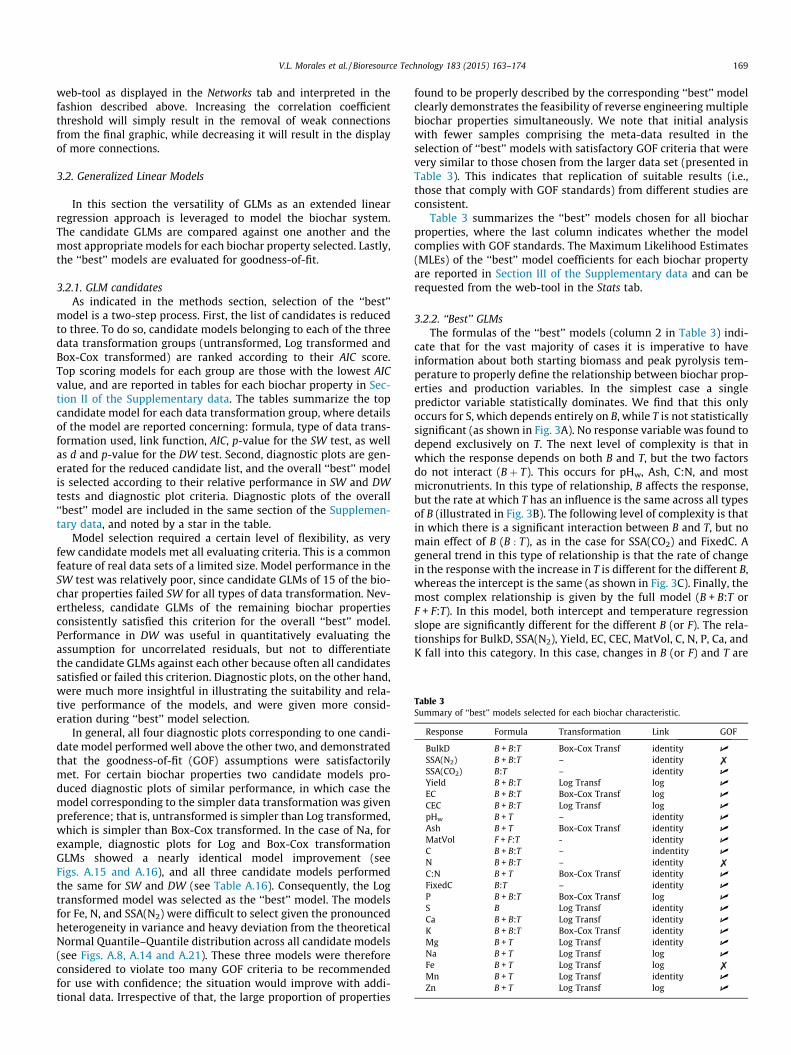
Table 3Summary of ‘‘best’’ models selected for each biochar characteristic.

Response Formula Transformation Link GOF

BulkD B + B:T Box-Cox Transf identity U

SSA(N2) B + B:T – identitySSA(CO2) B:T – identity U

Yield B + B:T Log Transf log U

EC B + B:T Box-Cox Transf log U

CEC B + B:T Log Transf log U

pHw B + T – identity U

Ash B + T Box-Cox Transf identity U

MatVol F + F:T - identity U

C B + B:T – indentity U

N B + B:T – identityC:N B + T Box-Cox Transf identity U

FixedC B:T – identity U

P B + B:T Box-Cox Transf log U

S B Log Transf identity U

Ca B + B:T Log Transf identity U

K B + B:T Box-Cox Transf identity U

Mg B + T Log Transf identity U

Na B + T Log Transf log U

Fe B + T Log Transf logMn B + T Log Transf identity U

Zn B + T Log Transf log U

V.L. Morales et al. / Bioresource Technology 183 (2015) 163–174 169

web-tool as displayed in the Networks tab and interpreted in thefashion described above. Increasing the correlation coefficientthreshold will simply result in the removal of weak connectionsfrom the final graphic, while decreasing it will result in the displayof more connections.

3.2. Generalized Linear Models

In this section the versatility of GLMs as an extended linearregression approach is leveraged to model the biochar system.The candidate GLMs are compared against one another and themost appropriate models for each biochar property selected. Lastly,the ‘‘best’’ models are evaluated for goodness-of-fit.

3.2.1. GLM candidatesAs indicated in the methods section, selection of the ‘‘best’’

model is a two-step process. First, the list of candidates is reducedto three. To do so, candidate models belonging to each of the threedata transformation groups (untransformed, Log transformed andBox-Cox transformed) are ranked according to their AIC score.Top scoring models for each group are those with the lowest AICvalue, and are reported in tables for each biochar property in Sec-tion II of the Supplementary data. The tables summarize the topcandidate model for each data transformation group, where detailsof the model are reported concerning: formula, type of data trans-formation used, link function, AIC, p-value for the SW test, as wellas d and p-value for the DW test. Second, diagnostic plots are gen-erated for the reduced candidate list, and the overall ‘‘best’’ modelis selected according to their relative performance in SW and DWtests and diagnostic plot criteria. Diagnostic plots of the overall‘‘best’’ model are included in the same section of the Supplemen-tary data, and noted by a star in the table.

Model selection required a certain level of flexibility, as veryfew candidate models met all evaluating criteria. This is a commonfeature of real data sets of a limited size. Model performance in theSW test was relatively poor, since candidate GLMs of 15 of the bio-char properties failed SW for all types of data transformation. Nev-ertheless, candidate GLMs of the remaining biochar propertiesconsistently satisfied this criterion for the overall ‘‘best’’ model.Performance in DW was useful in quantitatively evaluating theassumption for uncorrelated residuals, but not to differentiatethe candidate GLMs against each other because often all candidatessatisfied or failed this criterion. Diagnostic plots, on the other hand,were much more insightful in illustrating the suitability and rela-tive performance of the models, and were given more consid-eration during ‘‘best’’ model selection.

In general, all four diagnostic plots corresponding to one candi-date model performed well above the other two, and demonstratedthat the goodness-of-fit (GOF) assumptions were satisfactorilymet. For certain biochar properties two candidate models pro-duced diagnostic plots of similar performance, in which case themodel corresponding to the simpler data transformation was givenpreference; that is, untransformed is simpler than Log transformed,which is simpler than Box-Cox transformed. In the case of Na, forexample, diagnostic plots for Log and Box-Cox transformationGLMs showed a nearly identical model improvement (seeFigs. A.15 and A.16), and all three candidate models performedthe same for SW and DW (see Table A.16). Consequently, the Logtransformed model was selected as the ‘‘best’’ model. The modelsfor Fe, N, and SSA(N2) were difficult to select given the pronouncedheterogeneity in variance and heavy deviation from the theoreticalNormal Quantile–Quantile distribution across all candidate models(see Figs. A.8, A.14 and A.21). These three models were thereforeconsidered to violate too many GOF criteria to be recommendedfor use with confidence; the situation would improve with addi-tional data. Irrespective of that, the large proportion of properties

found to be properly described by the corresponding ‘‘best’’ modelclearly demonstrates the feasibility of reverse engineering multiplebiochar properties simultaneously. We note that initial analysiswith fewer samples comprising the meta-data resulted in theselection of ‘‘best’’ models with satisfactory GOF criteria that werevery similar to those chosen from the larger data set (presented inTable 3). This indicates that replication of suitable results (i.e.,those that comply with GOF standards) from different studies areconsistent.

Table 3 summarizes the ‘‘best’’ models chosen for all biocharproperties, where the last column indicates whether the modelcomplies with GOF standards. The Maximum Likelihood Estimates(MLEs) of the ‘‘best’’ model coefficients for each biochar propertyare reported in Section III of the Supplementary data and can berequested from the web-tool in the Stats tab.

3.2.2. ‘‘Best’’ GLMsThe formulas of the ‘‘best’’ models (column 2 in Table 3) indi-

cate that for the vast majority of cases it is imperative to haveinformation about both starting biomass and peak pyrolysis tem-perature to properly define the relationship between biochar prop-erties and production variables. In the simplest case a singlepredictor variable statistically dominates. We find that this onlyoccurs for S, which depends entirely on B, while T is not statisticallysignificant (as shown in Fig. 3A). No response variable was found todepend exclusively on T. The next level of complexity is that inwhich the response depends on both B and T, but the two factorsdo not interact (Bþ T). This occurs for pHw, Ash, C:N, and mostmicronutrients. In this type of relationship, B affects the response,but the rate at which T has an influence is the same across all typesof B (illustrated in Fig. 3B). The following level of complexity is thatin which there is a significant interaction between B and T, but nomain effect of B (B : T), as in the case for SSA(CO2) and FixedC. Ageneral trend in this type of relationship is that the rate of changein the response with the increase in T is different for the different B,whereas the intercept is the same (as shown in Fig. 3C). Finally, themost complex relationship is given by the full model (B + B:T orF + F:T). In this model, both intercept and temperature regressionslope are significantly different for the different B (or F). The rela-tionships for BulkD, SSA(N2), Yield, EC, CEC, MatVol, C, N, P, Ca, andK fall into this category. In this case, changes in B (or F) and T are

170 V.L. Morales et al. / Bioresource Technology 183 (2015) 163–174

not trivial, as the relationship permits the greatest level of flexibil-ity and rules out any general trends (as in Fig. 3D).

For the three simplest relationships (B, B + T, and B:T), achange in B does not affect the response order relative to theother types of B. Conversely, for the most complex relationship(B + B:T or F + F:T), a change in biomass affects the response insuch a way that it crosses over responses from other biomasstypes as T changes; thereby not necessarily maintaining the rela-tive order among the different types of biomass. This assessmentof multiple predictor variable influence corroborates the percep-tion that biochar properties are deeply shaped by the collectiveeffect of both production variables, whether additive and/orinteractive. Furthermore, it warrants against statistical bias thatis introduced when biochar production decisions are based onthe dominance of a single variable on a biochar property ofinterest. Interestingly, only the ‘‘best’’ model for MatVol favoredthe nested starting biomass, F. All other ‘‘best’’ models per-formed better when this information was entered in its moredetailed form, B.

The frequency in response variable transformation for theselected ‘‘best’’ models (column 3 in Table 3) indicates that a min-ority of the data are Normally distributed and meet the constantvariance assumption. Most responses require power-transforma-tion to stabilize their variance. Specifically, 7 response variableswere satisfactorily modeled without transformation of the respon-se values, while 9 others needed Log transformation and theremaining 6 required the more advanced Box-Cox transformation.This observation draws attention to the fact that non-constantvariance is ubiquitous in the characteristics of biochar, which

Fig. 3. Formula interpretation for GLMs of link identity. (A) Res

requires transformation of the response variable to comply withNormality assumptions. Depictions of different functional shapesare presented in Fig. 4 for models sharing the same formula(B + T) and identity link. In this figure, (A) is the reference for theuntransformed response for pHw, (B) is the Log transformedresponse for Mn, and (C) is the Box-Cox transformed response forAsh. In these plots, it is evident that the untransformed data havea perfectly linear relationship. In contrast, Log and Box-Cox trans-formations are suitable to describe non-linear behavior associatedwith a more cumbersome relationship between biochar propertiesand production variables.

Similarly, the prevalence of non-linear link functions in the‘‘best’’ model population (column 4 in Table 3) exposes the com-mon violation of the linearity assumption. It is interesting thatall 7 responses that demonstrated constant variance (i.e., notrequiring data transformation) also met the linearity assumption(favoring identity link function). This was also the case for 8 ofthe responses with unequal variances that required data transfor-mation. The remaining 7 responses required transformation toaddress variance instability and the log link function to furthercorrect for non-linearity. The log link function contributes to thenon-linear function shape of the response in a way that resemblesthat of Log and Box-Cox data transformation. Fig. 4 illustrates thiseffect for responses that have been Log transformed. The data in (B)satisfies the linearity assumption and is adequately modeled withthe identity link function. In contrast, the property in (D) needs alog link function to adjust for non-linearity. In short, both non-Gaussian and non-linear features were found to be ubiquitous inthe biochar system.

p � B. (B) Resp � B + T. (C) Resp � B:T. (D) Resp � B + B:T.

Fig. 4. Data transformation interpretation for GLMs of link identity and Formula B + T. (A) Untransformed. (B) Log transformed. (C) Box-Cox transformed. (D) Log transformedof link log.

V.L. Morales et al. / Bioresource Technology 183 (2015) 163–174 171

3.3. Biochar Engineering: the web-tool

The Biochar Engineering tool is an integrated calculator for thebiochar models in Table 3. The web-tool can be navigated throughthe various tabs on display at the top of the page. The About tabintroduces the tool, the Graphic and Table tabs contain the modelresults, the Stats tab summarizes individual model parameters,and the Networks tab displays networks of correlated biochar prop-erties. The side bar panel is always visible and can be modified atany time to re-run the model with new input variable values forbiomass, peak temperature, and confidence coefficient, requestthe statistical summary of a specific response model, set a correla-tion coefficient cutoff for the networks, and download the outputof any tab. The model output for the user-defined production vari-ables is automatically generated and updated in the Graphic andTable tabs. Correlation networks are similarly updated in the Net-works tab for newly defined correlation coefficients. Ultimately,this information can be used to select production variable valuesthat yield biochar with the most desirable set of properties forthe user, thereby facilitating the possibility to efficiently engineerbiochar resources to meet multiple agricultural demands.

3.4. Using GLMs and web-tool to engineer a biochar

Recommendations for the use of the GLMs in Table 3 cannot begeneralized because they depend on the particular set of properties

needed from biochar to mitigate deficiencies in a specific soil orcrop, as well as on the type of biomass available and limitationsof the pyrolysis unit. Rather than attempting to examine all possi-ble scenarios, this section presents two examples that demonstratehow the GLMs and the web-tool can be used to engineer the hypo-thetical biochar described in Section 3.1 (requiring high pHw, highP and S, high SSA(CO2) and/or high Ash, and high Yield). In the firstexample we assume a situation where all production variables canbe modified, and identify the optimum combination of startingbiomass and temperature that return the desired qualities. In thesecond example we assume a situation where the type of startingbiomass is fixed (e.g., to concurrently dispose of a byproduct fromanother process), and determine the temperature that is most suit-able to obtain the desired qualities.

3.4.1. A worked example for total optimization of production variablesIn the case where all production variables can be modified, we

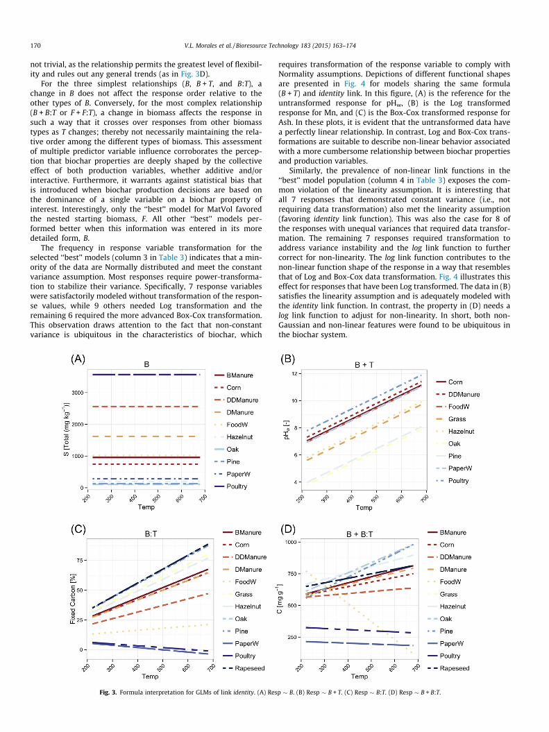
propose to refer to the prediction plots corresponding to theproperties of interest. Prediction plots for all properties analyzedin this study are included in Figs. A.24–A.45 of the Supplementarydata; see the particular case for pHw in Fig. 5. To facilitate inter-pretation of the model results, the predictive plots are presentedas composite figures where each subfigure corresponds to aunique type of starting biomass and the property of interestis plotted as a function of pyrolysis temperature. The predicted(mean) values are presented as a solid line, while regions

Fig. 5. Model predictions for pHw content (solid line) with confidence intervals for 75%, 85%, and 95% (dark gray, gray, light gray shading, respectively). Data points frommeta-data are overlain (solid circles).

172 V.L. Morales et al. / Bioresource Technology 183 (2015) 163–174

corresponding to 75%, 85%, and 95% confidence intervals areindicated by the shaded regions (dark gray, gray, light gray,respectively). For reference, the data points from the meta-dataare overlaid as solid circles.

We begin by analyzing Fig. 5 to identify the variables that candeliver biochar with high pHw. This figure shows that as T increasespHw increases, and this rate is constant across all B. Among the dif-ferent types of B included in the pHw model, biochars made frompoultry litter would typically result in the highest achievablepHw at any T, followed by digested dairy manure, corn, food waste,and paper waste. Next, we analyze the predictive plot for P(Fig. A.38). From this figure it is apparent that most Bs result in bio-chars with low P concentrations that are minimally variable withT; crossovers associated with the B:T coupling are mainly observedon the low T range. Notably, samples made from poultry litter con-tain the highest concentration of P (by orders of magnitude greaterthan samples of lowest P), with food waste and digested dairymanure following significantly behind in P concentration. Then,we examine the predictive plot for S (Fig. A.40), which is exclusive-ly dependent on B (in agreement with the ‘‘best’’ model formula forS in Table 3). It is easy to distinguish that poultry litter has thehighest S content, followed by digested dairy manure and dairymanure. Next, we consider predictions for SSA(CO2) (Fig. A.41),which also show a general increase in response with T at rates thatdepend on B (cf. formula B:T for the ‘‘best’’ SSA(CO2) model). Fromthese predictions we identify that hazelnut, pine and oak producethe highest possible SSA(CO2), which is enhanced as T is increased.Conversely, the predictive plot for Ash (Fig. A.24) indicates that thisproperty is typically around 30% and generally increases with T.Paper waste, poultry litter and food waste are ranked highest

among the B types to show high ash at all T levels. Lastly, the pre-dictive plot for Yield (Fig. A.44) demonstrates a pronouncedlydecreasing trend with increasing T for all B types, with crossoversthroughout, as expected from the ‘‘best’’ model formula B + B:Tgiven in Table 3 for Yield. It is evident that biochars from paperwaste and poultry litter produce the highest yield for the rangeof T investigated.

Based on the above observations, we conclude that poultry lit-ter pyrolyzed at T above 500 �C will return a biochar that meetsmost of the needed hypothetical properties. More concrete recom-mendations of T will depend on the producer’s choice to compro-mise between Ash and Yield, which have opposing trends with T.One way to facilitate this decision is to refer to the predictionsmade by the Biochar Engineering web-tool at various temperatures.By specifying in the side bar panel the biomass (poultry), peak tem-perature (a value in the range 500–600 �C), and a satisfactory con-fidence coefficient (e.g., 0.8), the web-tool automatically generatesa table (located in the Table tab) that summarizes the expected bio-char properties for the input variables. For discrete temperatures at500, 550, and 600 �C, the biochar would be expected to have an Ashcontent of 56.60%, 61.31%, and 66.4%, and Yield of 65.76%, 64.38%,and 63.03%, respectively. Considering that Ash is increased by 10%and Yield is only reduced by 2% when T is increased from 500 to600 �C, one might accept the small penalty in yield for gainingmore ash. Assuming all other considerations are satisfactory in thishypothetical scenario, one could conclude that the customized bio-char with the above listed characteristics is best produced bypyrolyzing poultry litter at 600 �C. For a comprehensive outlookon the expected range of all 22 physico-chemical properties, theuser may refer to the output generated in the Graphic or Table tabs

Fig. 6. Interface of the Biochar Engineering tool. Model output compiled in the Table tab.

V.L. Morales et al. / Bioresource Technology 183 (2015) 163–174 173

of the web-tool, and save the results with the download buttons forfuture reference.

3.4.2. A worked example for restrictions in starting biomassA similar approach to that followed in the first example can be

used to engineer a biochar for cases in which the type of biomass isfixed. Take for instance a corn farm, which is interested in sellingits corn stover resources as high quality biochar because livestockfeed and bioenergy prices are low. The properties required fromthe biochar, as specified by the client, are assumed to be the sameas those for the hypothetical biochar considered above. In this case,the farmer or pyrolysis contractor would be referred to the web-tool directly. In the side bar panel, the biomass should be set tocorn and a suitable confidence coefficient selected (e.g., 0.8). Thepeak temperature slider can then be used to study the changes inbiochar properties with temperature, as the only production vari-able that can be adjusted. The model output results can be moni-tored in either the Graphic tab (bar plots indicate predictedvalues with error bars marking the confidence interval range) orin the Table tab (table summary of predicted values with their cor-responding standard error and confidence interval). By shifting thepeak temperature slider from low to high temperatures it is evi-dent that Yield is diminished, SSA(CO2), pHw, Ash, and P are inten-sified, and S remains constant. Assuming in addition to therequired biochar properties that in order to make a profit, the Yieldshould be at least 30%, we can conclude that the corn stover shouldbe pyrolyzed at 467 �C, so the lower end of the expected yieldrange is above 30%. The Table tab of the web-tool (see screenshotin Fig. 6) summarizes the expected value and confidence interval

for each biochar property, according to the production variablesspecified. For corn pyrolyzed at 467 �C, the estimated range (with80% confidence level) for the desired properties is: 8.6–9.9 pHw,1647–2214 Total (mg/kg) P, and 633.1–869.9 Total (mg/kg) S,330.6–450.6 m2/g SSA(CO2), 11.8–16.2% Ash, and 30.0–33.1% Yield.

4. Conclusion

Statistical results demonstrate that arbitrary choices of startingbiomass or peak pyrolysis temperature are unlikely to produce bio-char with prescribed physico-chemical properties. Generalized Lin-ear Models were used to quantify the combined effect that startingbiomass and peak temperature has on different biochar properties.These properties are typically non-Gaussian and exhibit non-lineardependence on the two predictor variables. Proper description ofmost biochar properties by GLMs demonstrates the feasibility toengineer biochar. A web-application of the GLMs together withcorrelation networks are offered as tools to guide biocharengineering.

Acknowledgements

The authors thank Dr. D.R. Fuka and Dr. M.P. Allan for advise onprograming and statistical methods, and Dr. S. Sohi and Dr. O.Mašek for valuable discussions. This study was financed in partby the Teresa Heinz Foundation for Environmental Research andProject Unicorn. V.L. Morales acknowledges support from MarieCurie International Incoming Fellowships (FP7-PEOPLE-2012-SoilArchnAg).

174 V.L. Morales et al. / Bioresource Technology 183 (2015) 163–174

Appendix A. Supplementary data

Supplementary data associated with this article can be found, inthe online version, at http://dx.doi.org/10.1016/j.biortech.2015.02.043.

References

Abe, F., 1988. The thermochemical study of forest biomass. Bull. For. For. Prod. Res.Inst. Jpn. 352, 1–95.

Atkinson, C.J., Fitzgerald, J.D., Hipps, N.A., 2010. Potential mechanisms for achievingagricultural benefits from biochar application to temperate soils: a review.Plant Soil 337, 1–18.

Beesley, L., Moreno-Jimenez, E., Gomez-Eyles, J., Harris, E., Robinson, B., Sizmur, T.,2011. A review of biochars’ potential role in the remediation, revegetation andrestoration of contaminated soils. Environ. Pollut. 159, 3269–3282.

Cao, X., Harris, W., 2010. Properties of dairy-manure-derived biochar pertinent to itspotential use in remediation. Bioresour. Technol. 101, 5222–5228.

Cao, X., Ma, L., Liang, Y., Gao, B., Harris, W., 2011. Simultaneous immobilization oflead and atrazine in contaminated soils using dairy-manure biochar. Environ.Sci. Technol. 45, 4884–4889.

Chapman, H., 1965. Cation-exchange capacity. In: Norman, A. (Ed.), Methods of SoilAnalysis. Part 2. Chemical and Microbiological Properties. Agronomymonograph, pp. 891–901.

Cordero, T., Marquez, F., Rodriguez-Mirasol, J., Rodriguez, J., 2001. Predictingheating values of lignocellulosics and carbonaceous materials from proximateanalysis. Fuel 80, 1567–1571.

Cornelissen, G., Gustafsson, Ö., Bucheli, T.D., Jonker, M.T.O., Koelmans, A.A., van Noort,P.C.M., 2005. Extensive sorption of organic compounds to black carbon, coal, andkerogen in sediments and soils: mechanisms and consequences for distribution,bioaccumulation, and biodegradation. Environ. Sci. Technol. 39, 6881–6895.

Cross, A., Sohi, S.P., 2011. The priming potential of biochar products in relation tolabile carbon contents and soil organic matter status. Soil Biol. Biochem. 43,2127–2134.

Enders, A., Hanley, K., Whitman, T., Joseph, S., Lehmann, J., 2012. Characterization ofbiochars to evaluate recalcitrance and agronomic performance. Bioresour.Technol. 114, 644–653.

Ennis, C.J., Evans, A.G., Islam, M., Ralebitso-Senior, T.K., Senior, E., 2011. Biochar:carbon sequestration, land remediation and impacts on soil microbiology. Crit.Rev. Environ. Sci. Technol. 42, 2311–2364.

Gaskin, J., Steiner, C., Harris, K., Das, K., Bibens, B., 2008. Effect of low-temperaturepyrolysis conditions on biochar for agricultural use. T. ASABE 51, 2061–2069.

Glaser, B., Lehmann, J., Zech, W., 2002. Ameliorating physical and chemicalproperties of highly weathered soils in the tropics with charcoal – a review.Biol. Fertil. Soils 35, 219–230.

Hossain, M., Strezov, V., Chan, K., Ziolkowski, A., Nelson, P., 2011. Influence ofpyrolysis temperature on production and nutrient properties of wastewatersludge biochar. J. Environ. Manage. 92, 223–228.

Joseph, S., Peacocke, C., Lehmann, J., Munroe, P., 2009. Developing a biocharclassification and test methods. In: Lehmann, J., Joseph, S. (Eds.), Biochar forEnvironmental Management: Science and Technology. Earthscan, London, pp.107–126.

Joseph, S.D., Camps-Arbestain, M., Lin, Y., Munroe, P., Chia, C.H., Hook, J., vanZwieten, L., Kimber, S., Cowie, A., Singh, B.P., Lehmann, J., Foidl, N., Smernik, R.J.,

Amonette, . An investigation into the reactions of biochar in soil. Austr. J. SoilRes. 48, 501.

Karaosmanoglu, F., Is�ggür-Ergüdenler, A., Sever, A., 2000. Biochar from the straw-stalk of rapeseed plant. Energy Fuel. 14, 336–339.

Karhu, K., Mattila, T., Bergstrom, I., Regina, K., 2011. Biochar addition to agriculturalsoil increased CH4 uptake and water holding capacity – results from a short-term pilot field study. Agric. Ecosys. Environ. 140, 309–313.

Keiluweit, M., Nico, P., Johnson, M., Kleber, M., 2010. Dynamic molecular structureof plant biomass-derived black carbon (biochar). Environ. Sci. Technol. 44,1247–1253.

Laird, D.A., Fleming, P., Davis, D.D., Horton, R., Wang, B., Karlen, D.L., 2010. Impact ofbiochar amendments on the quality of a typical midwestern agricultural soil.Geoderma 158, 443–449.

Lehmann, J., Pereira da Silva, J.J., Steiner, C., Nehls, T., Zech, W., Glaser, B., 2003.Nutrient availability and leaching in an archeological anthrosol and a ferralsolof the central amazon basin: fertilizer, manure and charcoal amendments. PlantSoil 249, 343–357.

Lehmann, J., Rillig, M.C., Thies, J.E., Masiello, C.A., Hockaday, W.C., Crowley, D., 2011.Biochar effects on soil biota – a review. Soil Biol. Biochem. 43, 1812–1836.

Loganathan, V.A., Feng, Y., Sheng, G.D., Clement, T.P., 2009. Crop-residue-derivedchar influences sorption, desorption and bioavailability of atrazine in soils. SoilSci. Soc. Am. J. 73, 967.

Major, J., Rondon, M., Molina, D., Riha, S.J., Lehmann, J., 2010. Maize yield andnutrition during 4 years after biochar application to a colombian savanna oxisol.Plant Soil 333, 117–128.

Mukherjee, A., Zimmerman, A., Harris, W., 2011. Surface chemistry variationsamong a series of laboratory-produced biochars. Geoderma 163, 247–255.

Myers, R.H., Montgomery, D.C., Vining, G.G., Robinson, T.J., 2010. Geleralized LinearModels With Applications in Engineering and the Sciences. John Wiley & SonsInc, Hoboken, New Jersey.

Nguyen, B.T., Lehmann, J., 2009. Black carbon decomposition under varying waterregimes. Org. Geochem. 40, 846–853.

Novak, J., Busscher, W., 2013. Selection and use of designer biochars to improvecharacteristics of Southeastern USA coastal plain degraded soil. In: Lee, J.W.(Ed.), Advanced Biofuels and Bioproducts. Springer, New York, pp. 69–96.

Novak, J.M., Busscher, W.J., Laird, D.A., Ahmedna, M., Watts, D.W., Niandow, M.A.,2009. Impact of biochar amendment on fertility of a southeastern coastal plainsoil. Soil Sci. 174, 105–112.

Rajkovich, S., Enders, A., Hanley, K., Hyland, C., Zimmerman, A.R., Lehmann, J., 2012.Corn growth and nitrogen nutrition after additions of biochars with varyingproperties to a temperate soil. Biol. Fertil. Soils 48, 271–284.

Sander, M., Pignatello, J.J., 2005. Characterization of charcoal adsorption sites foraromatic compounds: insights drawn from single-solute and bi-solutecompetitive experiments. Environ. Sci. Technol. 39, 1606–1615.

Spokas, K., Cantrell, K., Novak, J., Archer, D., Ippolito, J., Collins, H., Boateng, A., Lima,I., Lamb, M., McAloon, A., Lentz, R., Nichols, K., 2012a. Biochar: a synthesis of itsagronomic impact beyond carbon sequestration. J. Environ. Qual. 41, 973–989.

Spokas, K.A., Novak, J.M., Venterea, R.T., 2012b. Biochar’s role as an alternative n-fertilizer: ammonia capture. Plant Soil 350, 35–42.

Zhao, L., Cao, X., Mašek, O., Zimmerman, A., 2013. Heterogeneity of biocharproperties as a function of feedstock sources and production temperatures. J.Hazard. Mater. 256–257, 1–9.

Zhu, D., Kwon, S., Pignatello, J.J., 2005. Adsorption of single-ring organic compoundsto wood charcoals prepared under different thermochemical conditions.Environ. Sci. Technol. 39, 3990–3998.