REVENUE FOCUSED SEMI-PROTECTION FOR VOD...

REVENUE FOCUSED SEMI-PROTECTION FOR VOD SERVICE IN COST-EFFECTIVE DWDM NETWORKS

by

Kaiyan Jin B.Sc., Harbin Engineering University, 2003

A PROJECT SUBMITTED IN PARTIAL FULFILLMENT OF THE REQUIREMENTS FOR THE DEGREE OF

MASTER OF SCIENCE

In the School

of Computing Science

© Kaiyan Jin 2009

SIMON FRASER UNIVERSITY

Spring 2009

All rights reserved. This work may not be reproduced in whole or in part, by photocopy

or other means, without permission of the author.

ii

APPROVAL

Name: Kaiyan Jin

Degree: Master of Science

Title of Project: Revenue Focused Semi-protection for VOD Service in Cost-effective DWDM Networks

Examining Committee:

Chair: Dr. Dirk Beyer Assistant Professor, Computing Science

______________________________________

Dr. Joseph G. Peters Senior Supervisor Professor, Computing Science

______________________________________

Dr. Qianping Gu Supervisor Professor, Computing Science

______________________________________

Dr. Mohamed M. Hefeeda SFU Examiner Assistant Professor, Computing Science

Date Defended/Approved: ______________________________________

SIMON FRASER UNIVERSITYLIBRARY

Declaration ofPartial Copyriight LicenceThe author, whose copyright is declared on the title page of this work, has grantedto Simon Fraser University the right to lend this thesis, project or extended essayto users of the Simon Fraser University Library, and to make partial or singlecopies only for such users or in response to a request from the library of any otheruniversity, or other educational institution, on its own behalf or for one of its users.

The author has further granted permission to Simon Fraser University to keep ormake a digital copy for use in its circulating collection (currently available to thepublic at the "Institutional Repository" link of the SFU Library website<www.lib.sfu.ca> at: <http://ir.lib.sfu.ca/handle/1892/112>) and, without changingthe content, to translate the thesis/project or extended essays, if technicallypossible, to any medium or format for the purpose of preservation of the digitalwork.

The author has further agreed that permission for multiple copying of this work forscholarly purposes may bl~ granted by either the author or the Dean of GraduateStudies.

It is understood that copying or publication of this work for financial gain shall notbe allowed without the author's written permission.

Permission for public performance, or limited permission for private scholarly use,of any multimedia materials forming part of this work, may have been granted bythe author. This information may be found on the separately cataloguedmultimedia material and in the signed Partial Copyright Licence.

While licensing SFU to permit the above uses, the author retains copyright in thethesis, project or extendE~d essays, including the right to change the work forsubsequent purposes, including editing and publishing the work in whole or inpart, and licensing other parties, as the author may desire.

The original Partial Copyright Licence attesting to these terms, and signed by thisauthor, may be found in the original bound copy of this work, retained in theSimon Fraser University Archive.

Simon Fraser University LibraryBurnaby, BC, Canada

Revised: Fall 2007

iii

ABSTRACT

Dense Wavelength Division Multiplexing (DWDM) technology is an

important innovation to enable the network operators to utilize their optical

networks efficiently. By multiplexing more wavelengths into one fiber, the data

transmission rate of a fiber in DWDM networks is dramatically increased up to

Terabits per second (Tbps). However, network operators are still struggling with

the bandwidth shortage problems due to the explosion of data transmission

demands, especially the transmission of video content. In this project, we present

a survey of the research on cost-effective DWDM networks in terms of the

routing and wavelength assignment (RWA) and traffic grooming problems. In

addition, we extend a revenue focused semi-protection scheme, which uses the

failure statistics, revenue statistics, and bandwidth statistics of VOD service to

solve bandwidth shortage problems in DWDM ring networks. Our goal is to

provide network operators with guidelines on the design or upgrade of their

DWDM networks.

Keywords: DWDM, RWA, traffic grooming, VOD, revenue focused semi-

protection, linear programming (LP), statistics.

iv

ACKNOWLEDGEMENTS

First of all, I would like to express my deepest gratitude to my senior

supervisor, Dr. Joseph G. Peters, for his patient and great supervision and

support. This project would not be completed without his tremendous support

and inspirational guidance. Also, special thanks go to Dr. Qianping Gu and Dr.

Mohamed M. Hefeeda, who helped me come up with initial ideas for this project

and devoted time to the final defense of this project. furthermore, I want to thank

all the members on the project examination committee, including the chair, Dr.

Dirk Beyer.

Secondly, I would like to extend my gratitude to my friends and

colleagues, for their endless support and encouragement. Special thanks to

Grace Mao, Hui Qin, Kevin Ge, Linda Lin, Ming Hua, Paul Zheng, and Priscilla

Cao.

Last but not the least, I am grateful to my wife, my parents, my sister and

brother for their unchangeable love and support! Thank you for always being

there for me.

v

TABLE OF CONTENTS

Approval .............................................................................................................. ii

Abstract .............................................................................................................. iii

Acknowledgements ........................................................................................... iv

Table of Contents ............................................................................................... v

List of Figures ................................................................................................... vii

List of Tables ..................................................................................................... ix

Glossary .............................................................................................................. x

Notation .............................................................................................................. xi

1. Introduction ..................................................................................................... 1

2. Background and Related Work ..................................................................... 8

2.1 Concepts and Terminology ................................................................ 8

2.1.1 DWDM network foundation ............................................................. 8

2.1.2 Network protections on SONET/DWDM rings ............................... 12

2.1.3 Cost-effective problems in SONET/DWDM rings .......................... 14

2.2 Related Work.................................................................................... 17

2.2.1 Routing and wavelength assignment ............................................ 18

2.2.2 Traffic grooming ............................................................................ 19

3. Revenue Focused Semi-protection Models ............................................... 22

3.1 Semi-protected Application Scenarios .............................................. 22

3.2 A Semi-protection Scheme ............................................................... 24

3.2.1 Notation ........................................................................................ 26

3.2.2 Model assumptions and statement ............................................... 28

3.3 Off-line Approach: Optimal Approach .............................................. 31

3.4 On-line Approaches .......................................................................... 36

3.4.1 Random Approach ........................................................................ 37

3.4.2 Revenue Approach ....................................................................... 39

3.4.3 Bandwidth Approach ..................................................................... 40

3.4.4 Failure approach ........................................................................... 41

3.4.5 Failure/Revenue/Bandwidth Combination Approach..................... 42

4. Experiments and Performance Comparison .............................................. 46

4.1 Background Description for Experiments ......................................... 47

4.1.1 Determination of values for predictor variables ............................. 48

4.2 2k Experimental Design .................................................................... 51

vi

4.3 Two-factor Full Factorial Design ....................................................... 56

4.4 Result Comparison with Previous Research .................................... 62

4.5 Observations .................................................................................... 66

4.6 Specific Case Studies ...................................................................... 67

4.6.1 Case 1: Impact of factor � in Combination Approach .................... 67

4.6.2 Case 2: A case study to compare Optimal with Combination ....... 73

4.6.3 Case 3: A case study on the predictor variable �� .................. 74

4.6.4 Case 4: A case study for the time when failures happen .............. 77

4.7 Time Cost Analysis ........................................................................... 80

5. Conclusions and Future Work ..................................................................... 81

Bibliography ...................................................................................................... 83

vii

LIST OF FIGURES

Figure 1-1: Many rings form a mesh network in a VOD network. Two dark rings run parallelly; the light colored ring can run independently or exchange data with the dark ring; the dotted ring may or may not share the routes with the other two rings. The optical signals of VOD programs in rings are converted to electronic signals and delivered to end users in Hybrid Fiber-Coax (HFC) networks. .............. 4

Figure 2-1: A FDM system example. .................................................................... 9

Figure 2-2: A FDM wavelength distribution. .......................................................... 9

Figure 2-3: A TDM system example. .................................................................. 10

Figure 2-4 : Cost-dominant components in SONET/DWDM rings. ..................... 14

Figure 2-5: SADM usage in SONET/WDM with 4 nodes and 2 wavelengths......................................................................................... 16

Figure 3-1: A point-to-point DWDM ring network ................................................ 25

Figure 3-2: Algorithm to calculate revenue loss rate for Random Approach ....... 38

Figure 3-3: Algorithm to calculate revenue loss rate for Revenue Approach ...... 40

Figure 3-4: Algorithm to calculate revenue loss rate for Failure Approach ......... 42

Figure 3-5: Algorithm to calculate revenue loss rate for Combination Approach ............................................................................................. 45

Figure 4-1: Revenue loss rate (%) when F = 1. .................................................. 58





Figure 4-6: Revenue loss rate (%) comparison of our study (dark-color) with [3] (light-color) for Optimal Approach. .......................................... 64

Figure 4-7: Revenue loss rate (%) comparison of our study (dark-color) with [3] (light-color) for Combination Approach. ................................... 65

Figure 4-8: Revenue loss rate (%) comparison of our study (dark-color) with [3] (light-color) for Failure Approach. ............................................ 65

Figure 4-9: Revenue loss rate with varying α in Experiment 1 and Experiment 2 with different values of ��, ��. ................................... 69

viii

Figure 4-10: Performance of Optimal Approach with varying ��. .................. 75

Figure 4-11: Performance of Failure Approach with varying ��. ................... 76

Figure 4-12: Performance of Combination Approach with varying ��. .......... 76

Figure 4-13: Comparison of the influence of different failure distributions. ......... 79

ix

LIST OF TABLES

Table 1: Performance result comparison between algorithms [41]. k is the grooming factor and n is the number of nodes. ................................... 21

Table 2: List and comparison of values for predictor variables (predictor variables are labelled from A to E). ...................................................... 49

Table 3: Levels and signs for the 5 predictor variables. ...................................... 52

Table 4: Importance of factors in each approach in terms of proportion of the total variation. ................................................................................ 55

Table 5: Revenue loss rate (%) of all the approaches in the full factorial design. ................................................................................................. 57

Table 6: Values used in Experiment 1 and Experiment 2. .................................. 69

Table 7: Priority ranks for (c,f)-customers in Experiment 3 (α =0.01) and Experiment 4 (α =0.05). ....................................................................... 71

Table 8: Dropped traffic and revenue loss comparison between Experiment 3 (α =0.01) and Experiment 4 (α =0.05). .......................... 71

Table 9: Dropped traffic and revenue loss comparison when each failure happens. .............................................................................................. 73

x

GLOSSARY

ADM ATM BLSR DWDM FDM HD OADM RWA SADM SD SDH SONET TDM UPSR VOD WDM

Add/Drop Multiplexer Asynchronous Transfer Mode Bidirectional Line Switched Ring Dense Wavelength Division Multiplexing Frequency Division Multiplexing High Definition Optical Add/Drop Multiplexer Routing and Wavelength Assignment SONET Add/Drop Multiplexer Standard Definition Synchronous Digital Hierarchy Synchronous Optical Network Time Division Multiplexing Unidirectional Path Switched Ring Video on Demand Wavelength Division Multiplexing

xi

NOTATION

c � � �� revenue-ratio �� , �, �� customers ��, �, �� , �, �� , �, �� , �, �� triple-ratio ratio(c) �� , �� , ��

Class � customers categorized by revenue rate generated The number of interruptions a customer has experienced The total number of failures occurring in the operation period The revenue rate generated by a class � customer The ratio between the revenue rates of the three classes of customers The bandwidth required for each class � customer The time right before the tth failure happens in the operation period [ ��, ��] The group of class � customers at time �� who have experienced � interruptions The number of ��, �, ��-customers The traffic load caused by the ��, �, ��-customers The number of new ��-customers The traffic load caused by the new ��-customers The number of dropped ��, �, ��-customers when the tth failure happens The amount of dropped traffic load of ��, �, ��-customers when the tth failure happens The ratio of the number of initial ��-customers, denoted ��0,0,0�:��1,0,0�:��2,0,0� ! ": #: $ The initial ratio of the number of �� -customers to the number of �� % 1�-customers The probability of ��-customers watching a VOD program The probability of a ��, ��-customer unsubscribing from the service if the customer experiences another failure The priority value of a ��, ��-customer The capacity of one link in the ring

1

1. INTRODUCTION

Dense Wavelength Division Multiplexing (DWDM), as an evolution of the

conventional Wavelength Division Multiplexing (WDM), enables the network

operators to utilize their existing optical network bandwidth efficiently. By

multiplexing more wavelengths in a fiber, the data transmission rate in a fiber can

be increased to over 10Tbps. For example, up to 14Tbps bandwidth in a fiber

has been achieved in the laboratory [1] and up to 160 wavelength channels per

fiber are in operation today [2].

On the other hand, the explosive growth of data transmission demands

results in bandwidth shortage problems for network operators. The fast

increasing video content service demands are the major causes, such as various

TV programs, Video-on-Demand (VOD) services, and video conferences over

networks. In addition, to provide reliable services, network protection schemes

are applied, which requires extra bandwidth reserved in the event of network

failures. Unidirectional Path Switched Ring (UPSR) and Bidirectional Line

Switched Ring (BLSR), the two typical protections in SONET ring networks,

require extra free bandwidth that is the same as the bandwidth of the working

fibers. The reserved bandwidth works as a backup and enables full protection.

Traditionally, network operators might have forecast the bandwidth growth and

overbuilt their networks for long-term designs when they planned to set up their

networks. However, almost all operators’ predictions have failed to catch up with

2

the fast growing speed of video content service demands. To solve this problem,

network operators have begun to consider the possibility of short-term or long-

term upgrade plans to increase the bandwidth of their existing networks.

Generally speaking, there are two alternative upgrade plans to meet the

growing bandwidth requirements.

First, network operators can choose to lay more optical cables to increase

the total capacity. Although the price of optical cables is much cheaper than other

transmission media (e.g., copper cables, measured by the price per unit

bandwidth), this is still a costly option, considering all the expenses involved

including labour and maintenance cost, conduit lease, new connection

components, and the cable itself.

The other plan for network operators is to apply new technologies to utilize

their existing networks efficiently without laying down additional fibers. DWDM

networks make this possible and have been proved to be more cost-effective

than the first plan. The technology of DWDM efficiently utilizes the bandwidth of a

fiber by supporting multiple wavelengths transmitted simultaneously in one fiber.

However, in order to multiplex more wavelengths into one fiber, more powerful

and signal-sensitive transmission modules (primarily wavelength converters and

add/drop multiplexers (ADMs)) are required to identify any two close

wavelengths, which incurs high additional costs. Optical ADMs (OADMs) and

SONET ADMs (SADMs) are the two major types of multiplexers in SONET

networks. To build cost-effective DWDM networks, the key challenge is to

maximize the efficiency of existing equipment and fibers at minimum deployment

3

cost. The routing and wavelength assignment (RWA) problem and the traffic

grooming problem are the two main problems that must be solved to find optimal

solutions in DWDM networks. The objective of the RWA problem is to find the

communication paths for given connection requests and to assign paths

wavelengths so that the number of required wavelengths is minimized. The

objective of the traffic grooming problem is to realize the given connection

requests by minimizing the use of SADMs in SONET networks. We will focus on

these two problems and illustrate more details later in our project.

Either one of the above plans can be applied as a long-term upgrade

design to increase the bandwidth of networks and accommodate the

continuously growing bandwidth demand.

Nonetheless, with or without protection, both plans mentioned above

require a certain amount of financial investment for network upgrade and

deployment. Network operators who cannot afford such investment in the near

future can consider another option to maximize the utilization of their existing

networks without adding extra cost and losing revenue from network failures: a

revenue focused semi-protection scheme proposed and studied in this project.

Different from other protection schemes that require more reserved bandwidth to

protect the network connections in the event of a failure, our revenue focused

semi-protection scheme uses any free bandwidth in the working link to protect

the selected network connections in the failed link and focuses on minimizing the

revenue loss. Moreover, the revenue focused semi-protection scheme incurs no

4

extra hardware upgrade cost in DWDM networks in contrast to solutions of RWA

and traffic grooming problems.

This project aims at solving the bandwidth shortage problem for a cost-

effective network by considering using a revenue focused semi-protection

scheme in DWDM networks. The solution proposed in this project applies to

SONET/DWDM ring networks. When we refer to DWDM in this project, it should

be understood that it also refers to WDM. SONET/DWDM ring is one of the

fundamental infrastructures in most current backbone optical networks and its

deployment and maintenance cost is relatively low. SONET networks consist of

one or more rings that run parallelly or independently and cross-rings that form a

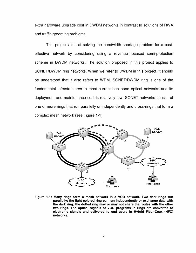
complex mesh network (see Figure 1-1).

Figure 1-1: Many rings form a mesh network in a VOD network. Two dark rings run parallelly; the light colored ring can run independently or exchange data with the dark ring; the dotted ring may or may not share the routes with the other two rings. The optical signals of VOD programs in rings are converted to electronic signals and delivered to end users in Hybrid Fiber-Coax (HFC) networks.

5

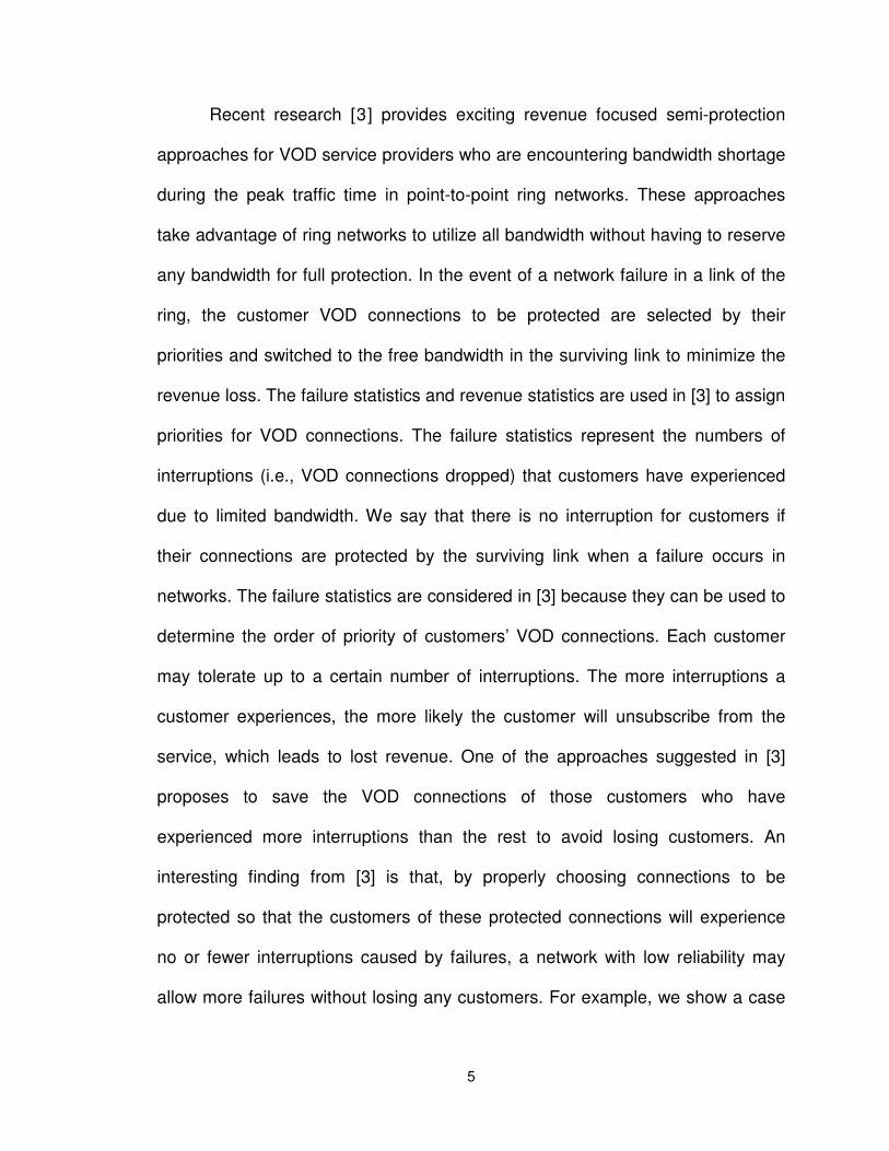
Recent research [3] provides exciting revenue focused semi-protection

approaches for VOD service providers who are encountering bandwidth shortage

during the peak traffic time in point-to-point ring networks. These approaches

take advantage of ring networks to utilize all bandwidth without having to reserve

any bandwidth for full protection. In the event of a network failure in a link of the

ring, the customer VOD connections to be protected are selected by their

priorities and switched to the free bandwidth in the surviving link to minimize the

revenue loss. The failure statistics and revenue statistics are used in [3] to assign

priorities for VOD connections. The failure statistics represent the numbers of

interruptions (i.e., VOD connections dropped) that customers have experienced

due to limited bandwidth. We say that there is no interruption for customers if

their connections are protected by the surviving link when a failure occurs in

networks. The failure statistics are considered in [3] because they can be used to

determine the order of priority of customers’ VOD connections. Each customer

may tolerate up to a certain number of interruptions. The more interruptions a

customer experiences, the more likely the customer will unsubscribe from the

service, which leads to lost revenue. One of the approaches suggested in [3]

proposes to save the VOD connections of those customers who have

experienced more interruptions than the rest to avoid losing customers. An

interesting finding from [3] is that, by properly choosing connections to be

protected so that the customers of these protected connections will experience

no or fewer interruptions caused by failures, a network with low reliability may

allow more failures without losing any customers. For example, we show a case

6

later in our experiments of a network that can have four failures without any

revenue loss even if no customer can tolerate two interruptions caused by

failures.

In Chapter 2, we survey research on cost-effective DWDM networks,

focusing on the RWA and traffic grooming problems. Solving these two problems

can help service providers minimize the use of some expensive components

when designing and upgrading cost-effective networks. We also present a review

of relevant heuristic algorithms and linear program models, which are basic tools

used to design or upgrade cost-effective networks by minimizing the use of costly

hardware devices or by maximizing network throughput.

In Chapter 3, we use additional statistics, the bandwidth statistics, to

extend the five semi-protection approaches proposed in [3] based on

assumptions and circumstances that are more realistic (e.g., more classes of

customers and different bandwidth usage). The five semi-protection approaches

are: Optimal, Random, Revenue, Failure, and Combination approaches. The

Optimal Approach is off-line approach because to solve the optimization problem,

it requires complete knowledge in advance, such as the pre-determined number

of total failures, and calculates the selection of protected network traffic before all

failures happen. The other approaches are on-line approaches because these

approaches selectively protect/drop the network traffic at the moment that a

failure happens. For the only off-line approach, Optimal Approach, we propose a

new linear programming (LP) model by adding the bandwidth statistics and

clarifying constraint functions for all variables. Moreover, we develop a new on-

7

line approach: Bandwidth Approach. Detailed algorithms to calculate the amount

of VOD traffic to be dropped for different classes of customers and revenue loss

rates for all the new and extended approaches are illustrated.

In Chapter 4, we conduct a 2k factorial experimental design to analyze the

effects of predictor variables and the full factorial design to analyze the

performance of all the approaches. The linear programming model always yields

global optimal performance (measured by revenue loss rate) based on complete

knowledge in advance. In practice, Optimal Approach may not be a good choice

since the number of failures cannot be pre-defined. Even though Combination

Approach shows the best overall performance among the on-line approaches by

locally minimizing the revenue loss, Bandwidth Approach proposed in this project

outperforms the other on-line approaches in some cases. In contrast to the

results in [3], by introducing the bandwidth statistics, our experimental results

show that Random Approach is not the worst approach whereas Revenue

Approach becomes the worst one. We compare our approaches with those in [3]

and find that our approaches can achieve less revenue loss than theirs. Some

performance results suggest that it is possible for service providers to achieve

zero revenue loss in their networks with relatively low reliability without having to

upgrade their networks and provide full protection.

We summarize the findings from this project and identify possible

directions for future work in Chapter 5.

8

2. BACKGROUND AND RELATED WORK

In this chapter, we introduce the basic concepts involved in this project

and investigate the literature on cost-effective DWDM networks, in particular,

RWA and traffic grooming problems.

2.1 Concepts and Terminology

DWDM was developed from WDM optical networks, and uses more

powerful and sensitive devices to space the light spectrum that is denser than

that in WDM. As a result, more wavelengths that carry the data traffic can be

multiplexed into a single optical fiber. DWDM has gained increasing interest in

many applications [4, 5] because it can be used to accommodate the rapidly

growing network bandwidth requirement, particularly in some backbone

networks.

2.1.1 DWDM network foundation

To fully appreciate the importance of DWDM, it is necessary to introduce

WDM because DWDM integrates the advantages of WDM, but utilizes the

bandwidth of a fiber more efficiently than WDM.

Before WDM networks, traditionally network operators provided their

services using some other multiplexing technologies, such as Frequency Division

Multiplexing (FDM) and Time Division Multiplexing (TDM) in most of their

copper cable or wireless networks.

9

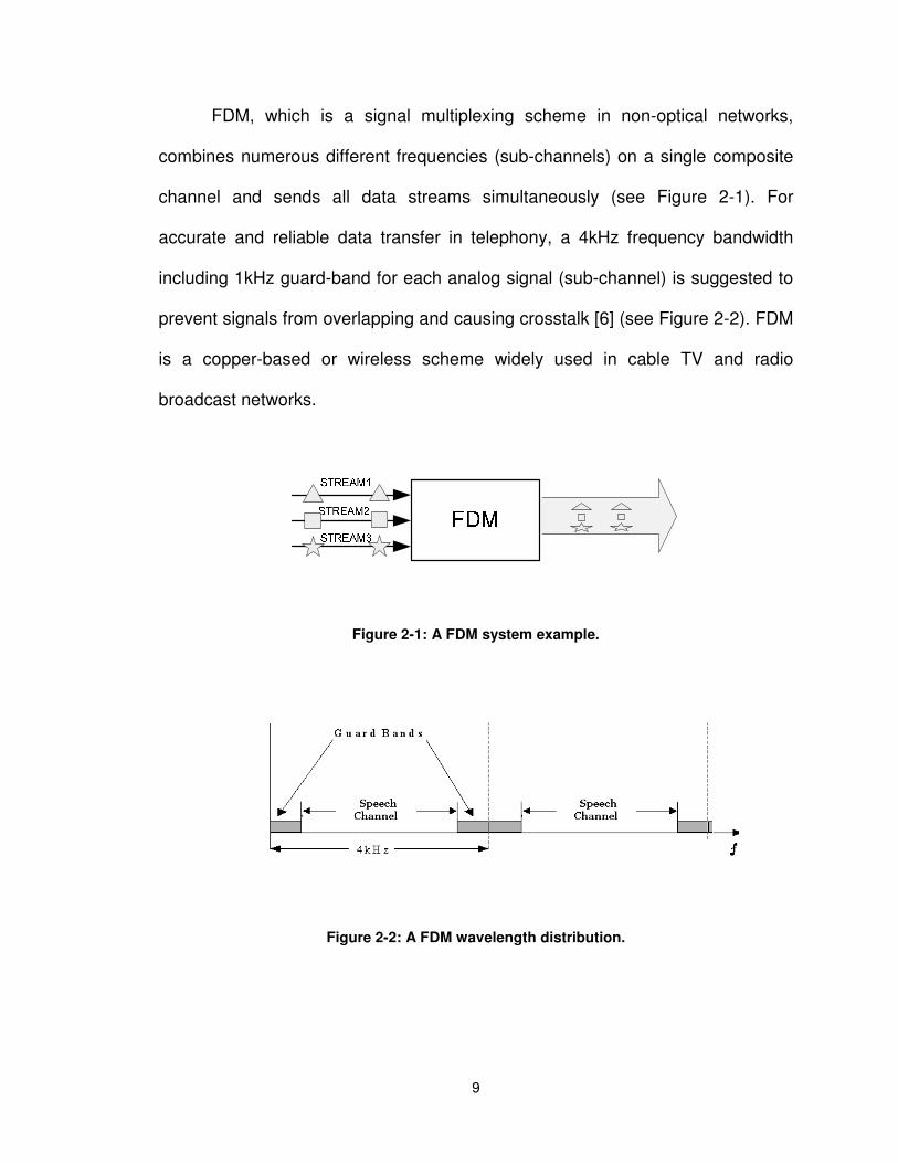
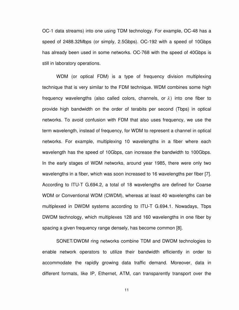
FDM, which is a signal multiplexing scheme in non-optical networks,

combines numerous different frequencies (sub-channels) on a single composite

channel and sends all data streams simultaneously (see Figure 2-1). For

accurate and reliable data transfer in telephony, a 4kHz frequency bandwidth

including 1kHz guard-band for each analog signal (sub-channel) is suggested to

prevent signals from overlapping and causing crosstalk [6] (see Figure 2-2). FDM

is a copper-based or wireless scheme widely used in cable TV and radio

broadcast networks.

Figure 2-1: A FDM system example.

Figure 2-2: A FDM wavelength distribution.

10

TDM, as illustrated in Figure 2-3, multiplexes data streams that may have

different transmission rates into one communication channel by assigning each

stream one or more slots in a time window. Thus, TDM enables us to utilize the

bandwidth of a channel more efficiently.

Figure 2-3: A TDM system example.

SONET (Synchronous Optical Network) and SDH (Synchronous Digital

Hierarchy) are sets of standards for synchronous transmission in optical

networks. SONET is the United States standard version set by American

National Standards Institute (ANSI) and SDH is the international version

published by the International Telecommunications Union (ITU). SONET and

SDH networks have been proved successful for their high performance and cost

effectiveness, and they are still under continuous development.

OC-1 (Optical Channel level 1) is the basic transmission module for

SONET and STM-1 (Synchronous Transport Module level 1, equivalent to OC-3

in SONET) for SDH. OC-1 and STM-1 transmit data streams at the speed of

51.84Mbps and 155.52Mbps respectively. The transmitter hierarchy OC-N has bit

rate of N &51.84Mbps by multiplexing several low speed data streams (e.g. N

11

OC-1 data streams) into one using TDM technology. For example, OC-48 has a

speed of 2488.32Mbps (or simply, 2.5Gbps). OC-192 with a speed of 10Gbps

has already been used in some networks. OC-768 with the speed of 40Gbps is

still in laboratory operations.

WDM (or optical FDM) is a type of frequency division multiplexing

technique that is very similar to the FDM technique. WDM combines some high

frequency wavelengths (also called colors, channels, or ' ) into one fiber to

provide high bandwidth on the order of terabits per second (Tbps) in optical

networks. To avoid confusion with FDM that also uses frequency, we use the

term wavelength, instead of frequency, for WDM to represent a channel in optical

networks. For example, multiplexing 10 wavelengths in a fiber where each

wavelength has the speed of 10Gbps, can increase the bandwidth to 100Gbps.

In the early stages of WDM networks, around year 1985, there were only two

wavelengths in a fiber, which was soon increased to 16 wavelengths per fiber [7].

According to ITU-T G.694.2, a total of 18 wavelengths are defined for Coarse

WDM or Conventional WDM (CWDM), whereas at least 40 wavelengths can be

multiplexed in DWDM systems according to ITU-T G.694.1. Nowadays, Tbps

DWDM technology, which multiplexes 128 and 160 wavelengths in one fiber by

spacing a given frequency range densely, has become common [8].

SONET/DWDM ring networks combine TDM and DWDM technologies to

enable network operators to utilize their bandwidth efficiently in order to

accommodate the rapidly growing data traffic demand. Moreover, data in

different formats, like IP, Ethernet, ATM, can transparently transport over the

12

optical layer in the DWDM network without the overhead of data encapsulation.

This technology development makes it feasible for network providers to deliver

diverse types of service over their networks, such as VOD service, video

conferencing, telecommunication, Internet, etc.

2.1.2 Network protections on SONET/DWDM rings

Service reliability, which is considered as part of QoS, requires service

providers to deploy protection architectures in their networks. Traditionally,

service providers offer various types of protection. These protection schemes can

be categorized into three classes: full protection, best-effort protection, and no

protection. We define a new protection scheme: revenue focused semi-protection

scheme.

In fully protected networks, paths with sufficient free bandwidth are set up

as the backup and can be used to transmit data traffic if the primary path is

interrupted. Typical fully protected architectures in SONET/DWDM rings are

unidirectional path switched ring (UPSR) and bidirectional line switched ring

(BLSR) [9 ]. In UPSR networks, one fiber works as the primary ring in the

clockwise direction and the other fiber works as the protection ring with a traffic

copy in the counter-clockwise direction. If a failure occurs in the path between

two adjacent nodes, the nodes can switch to the protected ring to receive the

data copy in the counter-clockwise direction. In BLSR rings, all traffic is

transmitted using 50% of the bandwidth of each of the two fibers that run in

opposite directions. Once a failure occurs in one of the fibers, the traffic is

switched to the free bandwidth in the other fiber.

13

Best-effort protection architectures have gained interest in some

research work [10,11]. Best-effort protection networks try to protect working

traffic as much as possible and/or maximize the revenue by using a mix of

carefully selected protected and unprotected schemes. Sridharan and Somani

[11] have used integer linear programming models to achieve the minimum cost

when a failure occurs in a network. Each link has been assigned a cost value,

and a currently working path disrupted by a failure will be assigned a second cost

value. The solution is to find the optimal path for rerouting with the minimum cost

in the event of a network failure. The survivability of a network, defined as the

capability of a network to provide continuous service in case of failures is

discussed in [11]. Gerstel and Ramaswami [11] reviewed different protection

schemes, such as BLSR, UPSR, and Mesh Line Protection. They then studied

different classes of protections from fully protected to unprotected and provided

network providers with suggestions regarding choosing the right scheme

depending on protection requirements and traffic types (e.g., deploying

protections in either IP layers or optical layers). The authors also considered

equipment cost and bandwidth efficiency as two important factors in a cost-

effective design.

Similar to best-effort protection schemes, our revenue focused semi-

protection scheme uses less bandwidth as backup than full protection schemes

but it requires no reserved bandwidth, traffic routes, or pre-defined levels of

protection. When failures occur in networks, traffic is selectively protected by any

14

free bandwidth in the other links to minimize the revenue loss caused by network

failures.

2.1.3 Cost-effective problems in SONET/DWDM rings

With DWDM technology, SONET networks can support large bandwidth

on a single fiber. However, the more wavelengths used, the more optical and

electronic multiplexing equipment required, which dominates the cost of

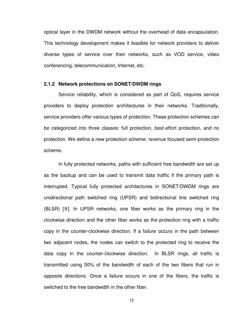
SONET/DWDM ring networks. Three costly components commonly used in a

SONET/DWDM ring network are shown in Figure 2-4: wavelength converters,

OADMs, and SADMs.

Figure 2-4 : Cost-dominant components in SONET/DWDM rings.

Converter: A converter receives a wavelength ('2 in Figure 2-4) and re-

transmits the data using a different wavelength ('3 in Figure 2-4). A converter

may be used when data traffic arrives on a wavelength that has already been

used in the fiber through which the converter sends data. Several studies [12,13]

have shown that using optical converters may reduce wavelength usage in some

15

cases, but it is still costly compared to the number of the wavelengths saved. To

simplify research problems in this project, we consider a point-to-point

communication request between two nodes and data transmitted along a

lightpath. A lightpath is an all-optical transmission path that is assigned a

wavelength, and there is no wavelength conversion or optical-electronic-optical

processing at intermediate nodes.

OADM: Optical Add/Drop Multiplexers offer the ability to selectively

add/drop a wavelength that carries only the data destined to or originating from a

node. Incoming wavelengths that do not contain data for the node will bypass the

OADM ('1 �� '2 bypass node 1 in Figure 2-4). There must be at least one

OADM at a node if there is traffic destined to or originating from this node.

SADM: SONET Add/Drop Multiplexers extract the low bit-rate streams

from a multiplexed wavelength and/or add a data stream in the same wavelength

for its destination node (see Figure 2-4). For example, a SADM drops an OC-3

data stream from a wavelength with an OC-12 integrated data stream, and adds

its own OC-3 data stream into the same wavelength and retransmits to its

destination. Therefore, a SADM is needed at a node only when a wavelength

channel carries incoming or outgoing low bit-rate streams for this node.

16

Figure 2-5: SADM usage in SONET/WDM with 4 nodes and 2 wavelengths.

Figure 2-5 (a) shows a unidirectional ring example without considering

minimizing the usage of SADMs. Suppose that the unidirectional communication

request set is {(1,2), (1,3), (1,4), (2,3), (2,4), (3,4)}, there are two given

wavelengths: '1 and '2, and each wavelength can aggregate two OC-3 data

streams denoted by solid and dotted lines. To realize all the requests without

concern for the SADM usage, a total of eight SADMs are used in Figure 2-5 (a)

(one OADM for each node is not shown in the figures). By properly using the

wavelength routing and assignment scheme, we can reduce the number of

SADMs to seven by bypassing node 2 for the wavelength '1, as shown in Figure

2-5 (b).

This example illustrates two of the optimization problems examined in

current research: routing and wavelength assignment (RWA) and traffic

grooming.

17

The RWA problem [14] is to find lightpaths for given connection requests

and to assign wavelengths to the lightpaths to meet the distinct wavelength

constraint and wavelength continuity constraint. The distinct wavelength

constraint requires that all lightpaths transmitted in the same fiber must be

assigned distinct wavelengths. The wavelength continuity constraint requires that

there be no wavelength conversion and electronic processing at intermediate

nodes. The objective of RWA is to realize all communication requests using a

minimum number of wavelengths or to maximize the traffic throughput using a

given number of wavelengths. If the routes for all requests are given in advance,

RWA problems can be reduced to WA (wavelength assignment) problems.

Traffic grooming in DWDM networks is a process to realize the given

traffic requests and minimize the use of SADMs by selectively grouping low data-

rate streams into a high data-rate output. A grooming factor refers to the number

of low data-rate streams that are multiplexed into one wavelength. For example,

in SONET/DWDM networks, an OC-48 SADM multiplexes four OC-12 low-rate

traffic streams into an OC-48 wavelength channel, and in this case, the grooming

factor is 4. As ADMs dominate the cost of DWDM networks, it is very important to

solve the traffic grooming problem in order to design cost-effective networks.

2.2 Related Work

To solve the RWA and traffic grooming problems, it is necessary to

optimize the use of wavelengths and SADMs. These problems have been proved

NP-hard [15,16,17] in mesh and ring networks. Thus, heuristic algorithms should

be applied to achieve the best possible performance. A lot of research has been

18

conducted on different network topologies, such as rings [16,27,33,34], mesh

networks [ 18 , 19 ,20 , 21 ], and trees [22 , 23 , 24 ] with or without considering

wavelength conversion. Some previous work [25] on coloring problems in graph

theory is also considered to provide solutions to RWA problems. Our review

focuses on the research for DWDM networks without wavelength conversion.

2.2.1 Routing and wavelength assignment

Ramaswami and Sivarajan [18] address the RWA optimization problem

using an integer linear program (ILP) model to maximize the number of

connections that are successfully routed for an arbitrary mesh network with a

given limited number of wavelengths. In addition, they derive an upper bound on

the number of connection requirements in their linear program (LP) model, by

relaxing the integrality constraints in ILP. An LP model in [12] considers RWA in

ring networks without wavelength conversion. The objective of the RWA LP

model is to minimize the number of required wavelengths. Variables are

introduced in these models to indicate whether a certain path is selected for one

connection and assigned one of the given wavelengths. The constraint functions

in these models include a constraint with a given number of wavelengths, and

distinct wavelength and wavelength continuity constraints.

More research on static traffic requests can be found in [26,27], which

proposed several heuristic algorithms to identify the proper lightpaths to be

assigned wavelengths so that the number of wavelengths is minimized. Some

greedy heuristic algorithms are presented and evaluated in [26] for both static

and dynamic traffic patterns with bounded and unbounded numbers of

19

wavelengths. The heuristic algorithms suggested in [26, 27] assign a given

wavelength to each lightpath from the longest one to the shortest one in order to

maximize the use of each wavelength. In [27], the authors give a lower bound on

the number of wavelengths required, ( ! )*+,�- . where N is the total number of

nodes, to realize all connection requests between all pairs of nodes in a DWDM

ring with two working fibers and two protection fibers.

The authors in [28] further proved that for a fully connected ring network,

which is a network having connections between all pairs of nodes, the lower

bound on the number of wavelengths required is ( ! )*+- . if N is even, and

( ! )*+,�- . if N is odd.

A RWA algorithm for connection maximization in undirected DWDM ring

networks with an approximation ratio 2/3 is presented in [29] and is considered to

be an improvement of �1 � �/ �-approximation in [30] (where e is the base of the

natural logarithm function). A 0�� -approximation algorithm is also given in [29] by

using the Chain-and-Matching technique for directed rings.

2.2.2 Traffic grooming

To solve the traffic grooming problem is to minimize the use of SADMs in

networks by multiplexing low-rate data streams into one high-rate wavelength

channel. In [31], the authors show that minimal number of wavelengths and

minimal number of SADMs are two objectives that cannot be achieved

simultaneously in their cases. It has been suggested that the traffic grooming

20

problem is more important than RWA when designing cost-effective DWDM

networks. For example, the researchers in [32,33] argue that the first-order

optimization goal should be to minimize the use of SADMs rather than to save

the number of wavelengths unless the wavelength limit is exceeded.

In [33], the authors derive a lower bound on the number of SADMs used

and an upper bound on the performance of two greedy heuristics, which are Cut-

First and Assign-First. The lower bound is described as

1 2 1345/67489: ! ∑ �<= % >= � min B<=, >=C= � , where <= is the total number of lightpaths departing from node k and >= is the

total number of lightpaths ended at node k. The lower bound is derived based on

the ideas that each pair of source and destination nodes requires one SADM and

the shared SADMs are bounded by min B<=, >=C. In [34], the authors achieve the same lower bound for the number of

SADMs, but argue that the performance analysis of the Assign-First algorithm in

[33] is incorrect and demonstrated so by giving a counter-example. Furthermore,

the authors propose another three greedy heuristics: Iterative Merging, Iterative

Matching, and Euler Cycle Decomposition.

Similar to research on RWA problems, some ILP models have been

proposed [35,36,37] for addressing traffic grooming problems.

For an arbitrary graph in UPSR rings with symmetric traffic patterns,

solutions to the k-Edge-Partitioning problem are used in [38,39,40,41] to solve

traffic grooming problems by partitioning a traffic graph G into subgraphs with at

21

most k edges. The basic idea common to all four papers is to minimize the

number of nodes, which may possibly decrease the number of connected

components in each subgraph, thereby decreasing the number of ADMs used.

Wang and Gu in [41] derive a better algorithm using an r-regular graph (all nodes

in a graph has the same degree r) and summarize the performance results of all

the relevant algorithms in one table (Table 1).

Table 1: Performance result comparison between algorithms [41]. k is the grooming factor and n is the number of nodes.

Required SADMs for even r Required SADMs for odd r Required wavelengths

Algorithm in [38] D|F�G�|�1 % 1H �I D|F�G�|�1 % 1H �I % 2 DF�G�H I Algorithm in [39] D|F�G�|�1 % 2H �I D|F�G�|�1 % 2H �I DF�G�H I Algorithm in [40] D|F�G�|�1 % 1H �I % J4L D|F�G�|�1 % 1H �I % J4L DF�G�H I Algorithm in [41] D|F�G�|�1 % 1H �I D|F�G�|�1 % 1H �I % � 32� % 1� � 1� DF�G�H I

22

3. REVENUE FOCUSED SEMI-PROTECTION MODELS

In this chapter, we develop revenue focused semi-protection models to

design cost-effective networks. Our goal is to minimize the revenue loss when

providing VOD service in a DWDM ring network by overcoming bandwidth

shortages without incurring any hardware upgrade costs.

3.1 Semi-protected Application Scenarios

Traditional DWDM ring networks use either non-protection or full

protection schemes. With the fast growth of video content transmission services,

many service providers face the problem of bandwidth shortage in their ring

networks. Common strategies that service providers have adopted to handle the

challenge of bandwidth shortage while minimizing the network updating cost or

revenue loss include: i) using new techniques to increase their bandwidth, such

as optical hardware upgrades in DWDM networks; ii) setting up additional optical

fibers to accommodate more network traffic; iii) giving up backup routes for full

protection and using all bandwidth as primary traffic deliverer; and iv) making no

new investment in existing networks and disconnecting traffic randomly at the

cost of possible revenue loss when failures occur in peak traffic time. None of the

above strategies is optimal: all the strategies will increase either cost or revenue

loss. Not much research has been done to improve these strategies using

customer statistics.

23

In this chapter, we develop revenue focused semi-protection approaches

to minimize the revenue loss by using customer statistics to determine the

priorities of all VOD connections. The solution achieved in this project provides

service providers with guidelines on the design or upgrade of cost-effective

networks. In practice, service providers have access to customer statistics from

customer surveys and online tracking records that suggest when a customer is

ordering or watching a VOD program. We believe that introducing the new

bandwidth statistic will not cost much more than only using the other two

statistics in [3].

Revenue statistics: Revenue statistics refer to subscription fees paid by

customers. We categorize customers into three classes: high-revenue,

moderate-revenue, and low-revenue customers.

Failure statistics: A customer experiences a network interruption when a

failure happens in a network and the VOD connection of the customer is chosen

to be dropped. The Failure statistic is the number of VOD service interruptions

that a customer experiences during a period of operation. Assuming that

customers can tolerate up to a certain number of network interruptions before

they unsubscribe from VOD programs, the more interruptions a customer

experiences, the more likely the customer will unsubscribe. Statistics can be

used to indicate customers’ tolerance of network interruptions; these statistics

are proportional to customers’ expectations of network reliability. It is reasonable

to assume that customers who pay higher subscription fees (i.e., higher revenue

customers) hold higher expectations. Therefore, experiencing the same number

24

of interruptions, higher revenue customers are more likely to unsubscribe than

lower revenue customers. In our project, to examine the effect of the number of

interruptions on revenue loss, we focus on revenue loss caused by customer

unsubscription from VOD service only after experiencing network interruptions.

Bandwidth statistics: Bandwidth statistics are the average bandwidths of

VOD programs required for different classes of customers. The authors [3] have

examined two different classes of customers (high- and low-revenue customers)

who have the same bandwidth usage. We assume that three different classes of

customers watch three different types of VOD programs: SD (Standard

Definition) VOD for low-revenue customers, DVD- quality VOD for moderate-

revenue customers, and HD (High Definition) VOD programs for high-revenue

customers. On average, SD, DVD-quality, and HD VOD programs occupy

3.75Mbps, 9.8Mbps, and 19Mbps bandwidths [42] respectively.

Some other impact factors (which are predictor variables in our

experimental designs) are evaluated, such as the probabilities customers are

watching when a failure happens, the composition ratio of the three classes of

customers, and the ranking impact factor for assigning the priorities to all

customers.

3.2 A Semi-protection Scheme

Similar to [3], we develop a semi-protection scheme for simple point-to-

point DWDM ring networks (Figure 3-1). In such a DWDM ring network, the

server node provides VOD service to a customer distribution node through the

25

two point-to-point links between the two nodes, and there is no specific backup

route reserved to protect the network when failures occur. Our scheme applies to

the situation when a failure occurs during the peak traffic time (e.g. the optical

fiber is broken) and the surviving link cannot accommodate the entire traffic load.

Consequently, some VOD connections have to be dropped, and some

connections are protected by the free bandwidth in the surviving link. To handle

this challenging situation, Gerstel et al. [3] proposed two semi-protection

schemes: non-preemptive protection and victimized protection.

Figure 3-1: A point-to-point DWDM ring network

In non-preemptive protection, when a failure happens in one of the two

links, a selection of connections in the broken link is saved by using the free

bandwidth in the surviving link. All the original traffic in the surviving link is

uninterrupted. In victimized protection, some VOD connections in the surviving

link are assigned lower priorities than selected connections from the broken link

26

and thus become victims to be dropped in order to free bandwidth for those

higher priority connections. Our project focuses on the victimized protection

scheme because the victimized protection scheme yields better performance

than the non-preemptive protection scheme in terms of minimizing revenue loss.

The victimized protection scheme selects connections to be protected based on

priorities assigned to all the connections in both surviving and broken links,

whereas the non-preemptive protection scheme selects based on the priorities

assigned to all the connections in the broken link only.

3.2.1 Notation

We use the following notation in our models and experiments.

�: Class � customers, where � N B0, 1, 2C represents low-revenue,

moderate-revenue and high-revenue customers respectively in our

simulation.

�: The number of interruptions a customer has experienced.

�: The total number of failures occurring in the operation period.

��: The revenue rate generated by a class � customer.

revenue-ratio: The revenue generation ratio between the revenue rates of

the three classes of customers, denoted �0�: �1�: �2�. ��: The bandwidth required for each class � customer.

27

��: � N B 0, 1, … , � % 1C, The time right before the tth failure happens in the

operation period [ ��, �� ], where �� represents the initial time in

the operation period before any failure happens.

��, �, ��-customers: The group of class � customers at time �� who have

experienced � interruptions. We also use ��-customers to mean

class c customer and ��, �� -customers to refer to the class c

customers who have experienced � interruptions.

��, �, ��: The number of ��, �, ��-customers.

��, �, ��: The traffic load caused by the ��, �, ��-customers when they are

watching VOD programs.

��: The number of new ��-customers joining the VOD service during

the period between two adjacent failures.

��: The traffic load caused by the new ��-customers when they are

watching VOD programs.

��, �, ��: The number of dropped ��, �, ��-customers when the tth failure

happens.

��, �, ��: The amount of dropped traffic load of ��, �, ��-customers when

the tth failure happens.

triple-ratio: The ratio of the number of initial ��-customers in the network

at �� ! 0, denoted ��0,0,0�:��1,0,0�:��2,0,0� ! ": #: $ . We also

28

assume that new customers subscribing to the service satisfy the

same ratio.

ratio(c): The initial ratio of the number of ��-customers to the number of

�� % 1� -customers, If ��0,0,0�:��1,0,0�:��2,0,0� ! ": #: $ , then,

��Q��0� ! "/# , and ��Q��1� ! #/$ . The new customers

subscribing to the service satisfy the same ratio.

��: The probability of a ��-customer watching a VOD program at the

peak traffic time.

��, ��: The probability of a ��, �� -customer unsubscribing from the

service if the customer is dropped at the next failure.

��, ��: The priority value that is assigned to a ��, �� -customer in

Combination Approach.

�: The capacity of one point-to-point link in the ring.

3.2.2 Model assumptions and statement

Our models do not apply to failures during non-peak traffic time. We

assume that there is no revenue loss during non-peak traffic time because all the

traffic can be saved by the free bandwidth in the surviving link and no customers

will experience interruptions. To simulate cases in peak traffic time, we develop

our models by adopting some similar assumptions to those described in [3]:

1. Initially, there is a certain number of �� -customers at time �� ,

satisfying the triple-ratio, which is the ratio among the numbers of

29

customers in each class. All the initial traffic is evenly distributed

between the two point-to-point links between the VOD server node and

customer distribution node in the ring. The total amount of the initial

traffic is equal to the bandwidth capacity of a link, thus half of the

bandwidth in each link is occupied by the initial traffic;

2. When a failure happens, some connections are dropped and there

may be customers who unsubscribe from the network. To ensure that

the total traffic always exceeds the bandwidth in the surviving link,

there are some new customers joining the network in the intervals

between adjacent pairs of failures, including the intervals of S ��, �� ] and [ �� , ��]. The number of new customers distributed across the

three different classes also satisfies the triple-ratio;

3. If no failure happens during the operation period S ��, �� ], the total

amount of initial traffic and the traffic caused by the new customers

should be equal to the full capacity of the two links at the end time

��; 4. All the traffic caused by all the new customers during the operation

period, which is equal to the capacity of one link, is evenly distributed

in the intervals between adjacent pairs of failures. Based on the triple-

ratio, the bandwidth consumption of each class of customers, and the

number of failures � during the operation period, the constant number

of new customers joining in each failure interval during one operating

period then can be determined. Despite our assumption, we

30

acknowledge that in reality, the number of new customers added to

each interval between two adjacent failures may not be constant

because the failures are not evenly distributed in real time. To get a

sense about how randomly occurring failures may affect revenue loss,

we also study a case that simulates three situations when varying

numbers of new customers join in the service in each interval between

two adjacent failures.

At time ��, we use ��, 0,0� to denote the initial number of ��-customers

who have never experienced any failures. �� is the time right before the tth failure,

where � ! 1,2… , � . Therefore, during the time S ��, ��T, there are in total �

failures. At any time �� , each �� -customer is watching VOD programs with

probability ��. The initial traffic load, denoted ��, 0,0�, is equal to the fixed

capacity � of one link. There is always a constant number of new customers,

��, joining the network and contributing the traffic load �� during the time

interval between adjacent failures. In order to ensure that the total number of

customers at any time exceeds the capacity of one link, but is not greater than

the total capacity of the two links at the end time �� , the total initial traffic

∑ ��, 0,0�UVW� ! � is evenly distributed in the two links, thus �/2 for each link. The

constant amount of traffic load ∑ ��UVW� ! X�� generated by the new

customers ��, is determined by the total number of failures in an experimental

period and will keep increasing the total traffic to 2� at the end time �� if no

customers leave. The number of initial ��-customers and all the new customers

31

added across the three different classes satisfy the � Q�YZ � ��Q�, and *�V,�,��*�V��,�,�� ![�V�[�V�� ! ��Q��, � ! B0,1C. The probability of a ��, �, ��-customer unsubscribing

from the network is ��, �� after they experience � % 1 interruptions. The

revenue loss rate then can be calculated with the revenue loss caused by all the

leaving customers divided by the total revenue when no customer leaves.

3.3 Off-line Approach: Optimal Approach

To achieve an optimal cost-effective semi-protection scheme, we extend

the linear programming model, which was developed in [3]. Our goal is to

minimize the total revenue loss rate at the end time �� by calculating the

optimal amount of dropped connections carefully selected using the customer

statistics. Therefore, ��, �, �� and ��, �, �� are the variables that need to be

determined in the model.

Suppose a �� -customer is watching a VOD program with probability

�� , and each customer who is watching the program is occupying

bandwidth ��. Then we have the following equation to describe the relation

between the number of ��, �, ��-customers and the amount of traffic caused by

these ��, �, ��-customers at any time ��. ��, �, �� ! ��, �, �� & �� & �� 1�,

�\Z Z � ! 0,1, 2, � ! 0,1, … , �, � ! 0,1, … , � % 1, � ] � *1.

*

1 No any customer experiences more than � � 1 failures at time �� , which is the time just before the �th failure happens, so � ] � throughout our project.

32

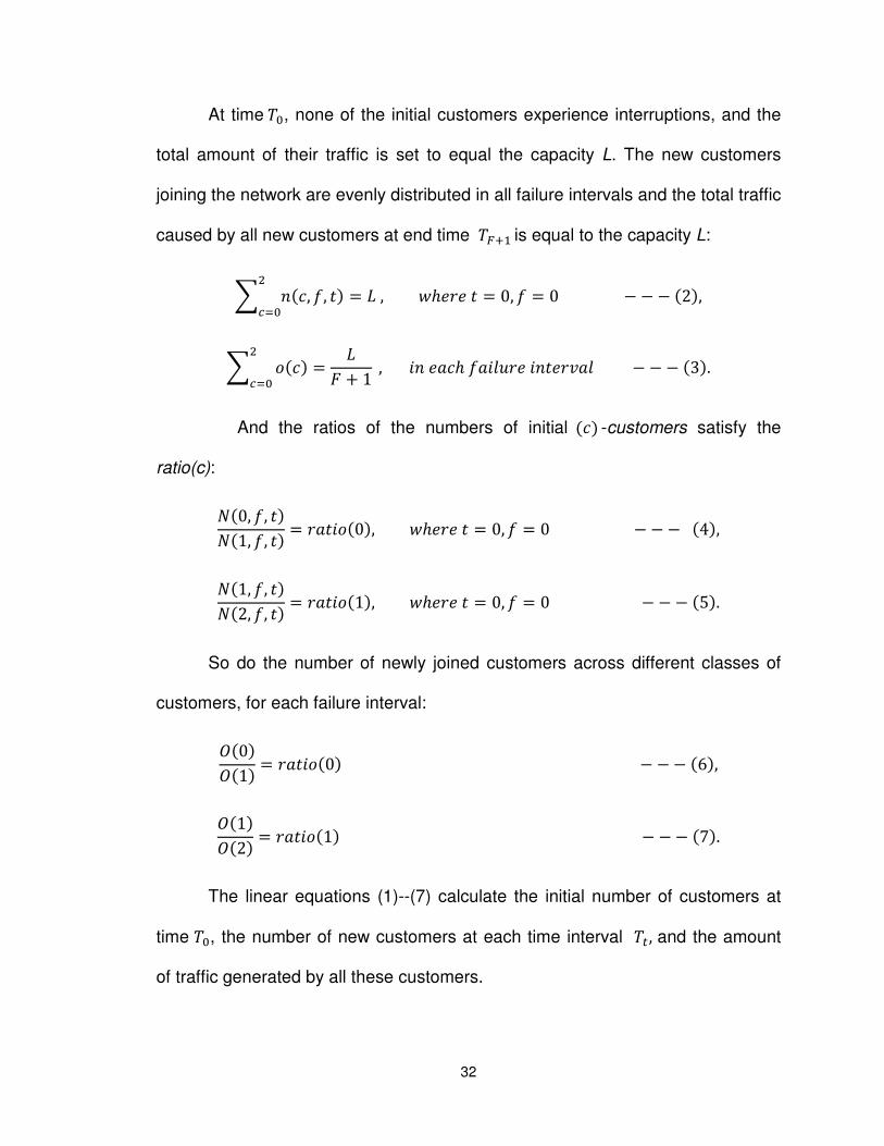
At time ��, none of the initial customers experience interruptions, and the

total amount of their traffic is set to equal the capacity L. The new customers

joining the network are evenly distributed in all failure intervals and the total traffic

caused by all new customers at end time �� is equal to the capacity L:

^ ��, �, �� ! � , �\Z Z � ! 0, � ! 0 UVW� � � � �2�,

^ �� ! �� % 1 , Q Z��\ ��QY� Z Q�Z _�Y UVW� � � � �3�.

And the ratios of the numbers of initial �� -customers satisfy the

ratio(c):

��0, �, ��1, �, �� ! ��Q��0�, �\Z Z � ! 0, � ! 0 � � � �4�, ��1, �, ��2, �, �� ! ��Q��1�, �\Z Z � ! 0, � ! 0 � � � �5�.

So do the number of newly joined customers across different classes of

customers, for each failure interval:

��0��1� ! ��Q��0� � � � �6�, ��1��2� ! ��Q��1� � � � �7�.

The linear equations (1)--(7) calculate the initial number of customers at

time ��, the number of new customers at each time interval ��, and the amount

of traffic generated by all these customers.

33

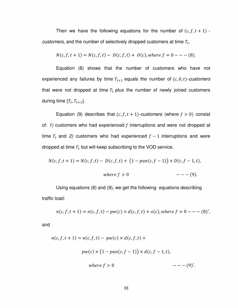
Then we have the following equations for the number of ��, �, � % 1� -

customers, and the number of selectively dropped customers at time ��. ��, �, � % 1� ! ��, �, �� , �, �� % ��,�\Z Z � ! 0 � � � �8�.

Equation (8) shows that the number of customers who have not

experienced any failures by time �� equals the number of ��, 0, ��-customers

that were not dropped at time �� plus the number of newly joined customers

during time S��, ��T. Equation (9) describes that ��, �, � % 1�-customers (where � d 0) consist

of: 1) customers who had experienced � interruptions and were not dropped at

time �� and 2) customers who had experienced � � 1 interruptions and were

dropped at time �� but will keep subscribing to the VOD service.

��, �, � % 1� ! ��, �, �� , �, �� % e1 � ��, � � 1�f & ��, � � 1, ��, �\Z Z � d 0 � � � �9�. Using equations (8) and (9), we get the following equations describing

traffic load:

��, �, � % 1� ! ��, �, �� & ��, �, �� % ��, �\Z Z � ! 0 � � � �8�h, and

��, �, � % 1� ! ��, �, �� & ��, �, �� % �� & e1 � ��, � � 1�f & ��, � � 1, ��,

�\Z Z � d 0 � � � �9�h.

34

The next step is to determine the amount of traffic caused by each group

of ��, �, ��-customers that we have to disconnect when the tth failure happens. We

assume that the fixed capacity of each link is L, and then the dropped traffic that

exceeds the capacity of one link caused by the tth failure can be calculated by:

^ ^ ��, �, ��,�iW�

UVW� ! max B0,^ ^ ��, �, �� C . �,�

iW�UVW�

Since we only model the situation during the peak traffic time when there

is not sufficient capacity in the surviving link for all VOD connections, some of the

connections have to be dropped if a failure occurs. Therefore, the above formula

can be simplified:

^ ^ ��, �, ��,�iW�

UVW� ! ^ ^ ��, �, �� 10�.�,�

iW�UVW�

So far, we have explained all the linear equations for the linear

programming model. Additional constraints for this model are introduced in (11)-

(12).

��, �, �� ] ��, �, �� 11�. The constraint (11) shows that at the time when the tth failure happens, the

amount of the dropped traffic cannot exceed the current traffic of ��, �, �� .

Moreover, all the variables in the model are non-negative numbers, so we have

��, �, �� 2 0 � � � �12�, and

��, �, �� ! 0, �\Z � ! � � � � �13�.

35

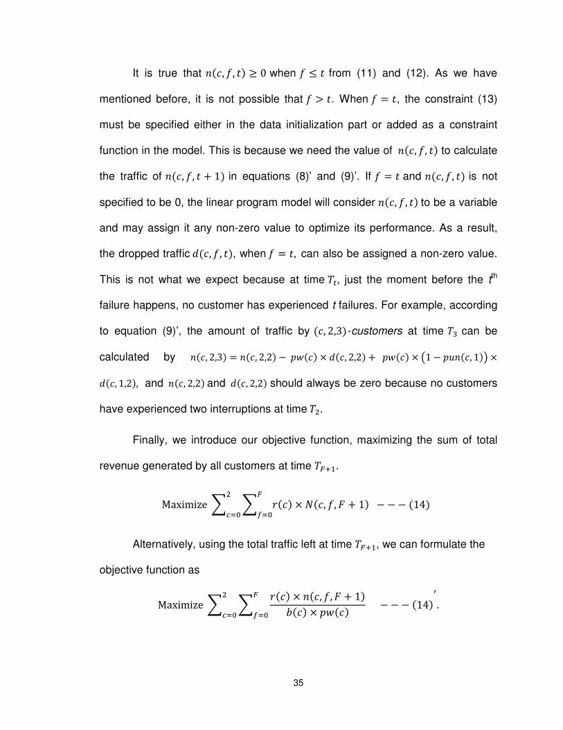
It is true that ��, �, �� 2 0 when � ] � from (11) and (12). As we have

mentioned before, it is not possible that � d �. When � ! �, the constraint (13)

must be specified either in the data initialization part or added as a constraint

function in the model. This is because we need the value of ��, �, �� to calculate

the traffic of ��, �, � % 1� in equations (8)’ and (9)’. If � ! � and ��, �, �� is not

specified to be 0, the linear program model will consider ��, �, �� to be a variable

and may assign it any non-zero value to optimize its performance. As a result,

the dropped traffic ��, �, ��, when � ! �, can also be assigned a non-zero value.

This is not what we expect because at time ��, just the moment before the tth

failure happens, no customer has experienced t failures. For example, according

to equation (9)’, the amount of traffic by ��, 2,3�-customers at time �l can be

calculated by ��, 2,3� ! ��, 2,2� � �� & ��, 2,2� % �� & e1 � ��, 1�f &��, 1,2�, and ��, 2,2� and ��, 2,2� should always be zero because no customers

have experienced two interruptions at time �U.

Finally, we introduce our objective function, maximizing the sum of total

revenue generated by all customers at time ��. Maximize ^ ^ �� & ��, �, � % 1� � � � �14� �

iW�UVW�

Alternatively, using the total traffic left at time ��, we can formulate the

objective function as Maximize ^ ^ �� & ��, �, � % 1�� & �� 14��

iW�UVW�

p.

36

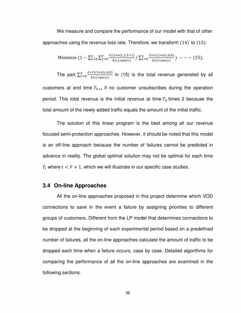
We measure and compare the performance of our model with that of other

approaches using the revenue loss rate. Therefore, we transform �14�′ to �15�. Minimize �1 � ∑ ∑ 6�V�&9�V,i,��7�V�&q5�V� /∑ U&6�V�&9�V,�,��7�V�&q5�V� �UVW� � � � �15��iW�UVW� , The part ∑ U&6�V�&9�V,�,��7�V�&q5�V� UVW� in (15) is the total revenue generated by all

customers at end time �� if no customer unsubscribes during the operation

period. This total revenue is the initial revenue at time �� times 2 because the

total amount of the newly added traffic equals the amount of the initial traffic.

The solution of this linear program is the best among all our revenue

focused semi-protection approaches. However, it should be noted that this model

is an off-line approach because the number of failures cannot be predicted in

advance in reality. The global optimal solution may not be optimal for each time

�� where � r � % 1, which we will illustrate in our specific case studies.

3.4 On-line Approaches

All the on-line approaches proposed in this project determine which VOD

connections to save in the event a failure by assigning priorities to different

groups of customers. Different from the LP model that determines connections to

be dropped at the beginning of each experimental period based on a predefined

number of failures, all the on-line approaches calculate the amount of traffic to be

dropped each time when a failure occurs, case by case. Detailed algorithms for

comparing the performance of all the on-line approaches are examined in the

following sections.

37

3.4.1 Random Approach

In Random Approach, all customers are assumed to be of the same

priority. We randomly select the VOD connections (for example, by randomly

selecting customer IDs from the customer database) to be dropped among

��, �, ��-customers when a failure occurs. Because no specific statistics are used

to assign priorities to customers, the algorithm to randomly select the protected

customers is similar to [3].

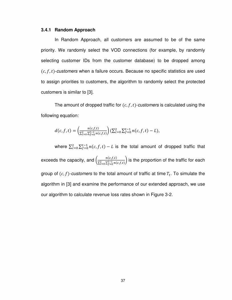
The amount of dropped traffic for ��, �, ��-customers is calculated using the

following equation:

��, �, �� ! s 9�V,i,��∑ ∑ 9�V,i,��tuvwxy+zxy { �∑ ∑ ��, �, ��,�iW�UVW� � ��, where ∑ ∑ ��, �, ��,�iW�UVW� � � is the total amount of dropped traffic that

exceeds the capacity, and s 9�V,i,��∑ ∑ 9�V,i,��tuvwxy+zxy { is the proportion of the traffic for each

group of ��, ��-customers to the total amount of traffic at time ��. To simulate the

algorithm in [3] and examine the performance of our extended approach, we use

our algorithm to calculate revenue loss rates shown in Figure 3-2.

38

In step 1, all data is initialized, including the initial traffic at time �� and

newly joined traffic during each interval. Step 3 calculates the current traffic for

each group of ��, �, ��-customers at time �� using the same functions (8)’ and (9)’

as in the linear programming model. The total traffic |�}��) is summed up at step

4 and is used to calculate the proportion of the traffic for ��, ��-customers to be

dropped at step 7. We only consider the case � r � % 1 at step 5 because the

last failure, that is, the Fth failure, happens right after time �� and there is no

traffic dropping at the end time ��. Step 8 specifies that the revenue loss rate,

which expresses our later experimental results, is the ratio of the actual total

revenue loss caused by all the customers who unsubscribed from the VOD

service to the expected total revenue assuming there is no unsubscription during

the experimental period.

1) data initialization;

2) for (t=1; t <= F+1; t++)

3) calculate the traffic ��, �, �� at time ��, for each c and f;

4) calculate |�}�� ! ∑ ∑ ��, �, ��,�iW�UVW� at time ��; 5) if t < F+1

6) � ��Z�_� ��Q�� ! |�}�� Q�#;

7) ��, �, �� ! � ��Z�_� ��Q�� 9�V,i,��8��, for each c and f ;

8) Output Z_Z�Z Y�|| ��Z ! �∑ ∑ ∑ ��&��,�,��&��,�� revenue_noleaving��!02�!0��W� ;

Figure 3-2: Algorithm to calculate revenue loss rate for Random Approach

39

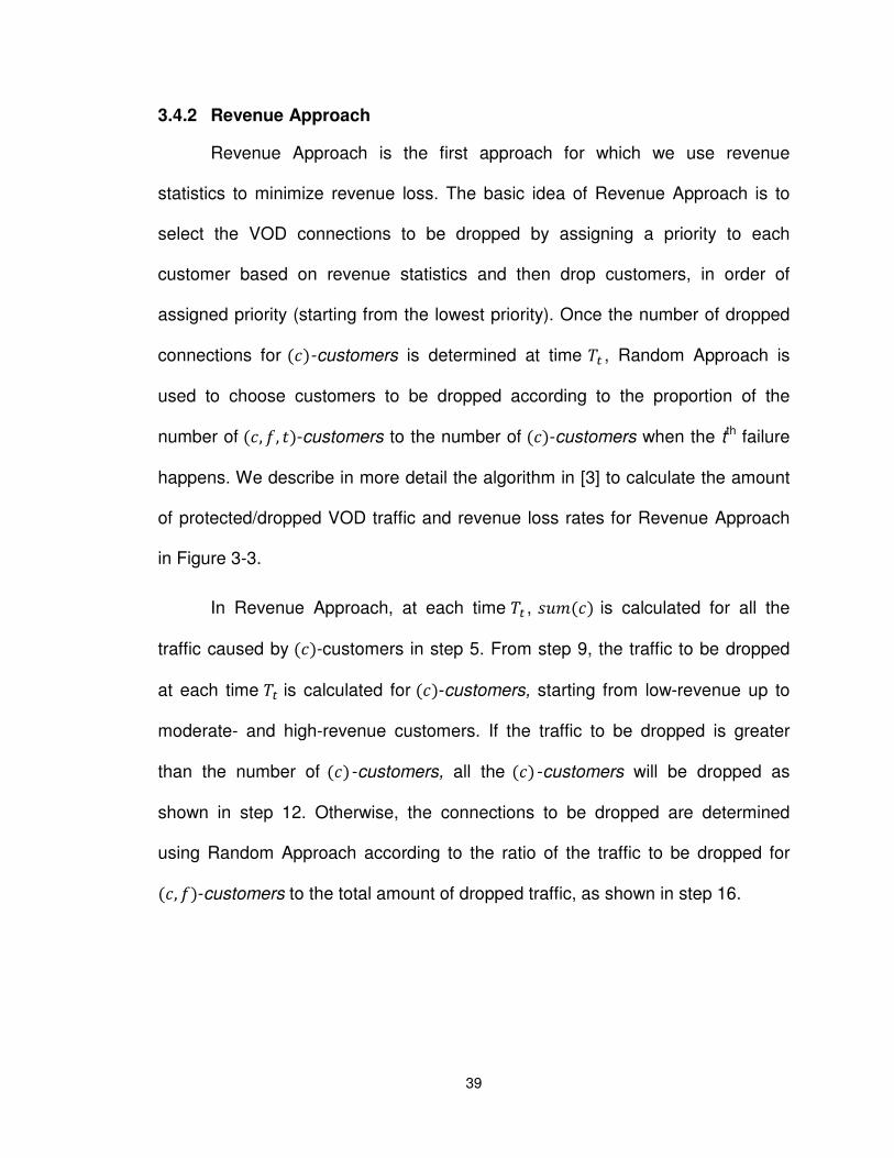
3.4.2 Revenue Approach

Revenue Approach is the first approach for which we use revenue

statistics to minimize revenue loss. The basic idea of Revenue Approach is to

select the VOD connections to be dropped by assigning a priority to each

customer based on revenue statistics and then drop customers, in order of

assigned priority (starting from the lowest priority). Once the number of dropped

connections for ��-customers is determined at time �� , Random Approach is

used to choose customers to be dropped according to the proportion of the

number of ��, �, ��-customers to the number of ��-customers when the tth failure

happens. We describe in more detail the algorithm in [3] to calculate the amount

of protected/dropped VOD traffic and revenue loss rates for Revenue Approach

in Figure 3-3.

In Revenue Approach, at each time �� , |�}�� is calculated for all the

traffic caused by ��-customers in step 5. From step 9, the traffic to be dropped

at each time �� is calculated for ��-customers, starting from low-revenue up to

moderate- and high-revenue customers. If the traffic to be dropped is greater

than the number of �� -customers, all the �� -customers will be dropped as

shown in step 12. Otherwise, the connections to be dropped are determined

using Random Approach according to the ratio of the traffic to be dropped for

��, ��-customers to the total amount of dropped traffic, as shown in step 16.

40

3.4.3 Bandwidth Approach

After introducing the bandwidth statistic, Bandwidth Approach is used to

maximize VOD connections to be saved by dropping connections that use more

bandwidth first. As mentioned earlier, one of our assumptions in this project is

that higher revenue customers use more bandwidth. Therefore, the priority

values assigned to VOD connections in Bandwidth Approach are ranked in the


2) for ( t = 1; t <= F+1; t++)

3) calculate the traffic ��, �, �� at time �� for each c and f;

4) calculate |�}�� ! ∑ ∑ ��, �, ��,�iW�UVW� at time ��; 5) calculate |�}�� ! ∑ ��, �, ��,�iW� at time �� for each c;

6) if t < F+1 // no drop for ��;

7) � ��Z�_� ��Q�� ! |�}�� Q�#;

8) temp = � ��Z�_� ��Q��; 9) for ( c = 0; c <= 2; c++)

10) if |�}�� ] �Z}�

11) for ( f = 0; f < t; f++)

12) ��, �, �� ! ��, �, ��; 13) �Z}� ! �Z}� � ��, �, ��; 14) else if |�}�� d �Z}�

15) for ( f = 0; f < t; f++)

16) ��, �, �� ! �Z}� � 9�V,i,��8��V� ; 17) �Z}� ! 0; 18) Output Z_Z�Z Y�|| ��Z !�∑ ∑ ∑ ��&��,�,��&��,�� revenue_noleaving��!02�!0��W�

Figure 3-3: Algorithm to calculate revenue loss rate for Revenue Approach

41

reverse order to those in Revenue Approach. The algorithm for Bandwidth

Approach is similar to the algorithm for Revenue Approach, which is shown in

Figure 3-3, except that we reverse the iteration in step 9 and run it from high

revenue to low to choose VOD connections to be dropped when a failure occurs.

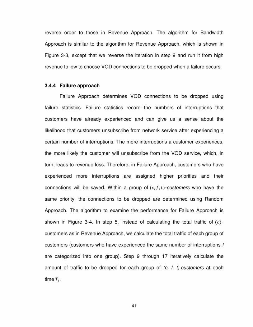
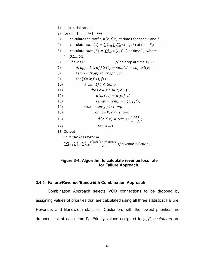
3.4.4 Failure approach

Failure Approach determines VOD connections to be dropped using

failure statistics. Failure statistics record the numbers of interruptions that

customers have already experienced and can give us a sense about the

likelihood that customers unsubscribe from network service after experiencing a

certain number of interruptions. The more interruptions a customer experiences,

the more likely the customer will unsubscribe from the VOD service, which, in

turn, leads to revenue loss. Therefore, in Failure Approach, customers who have

experienced more interruptions are assigned higher priorities and their

connections will be saved. Within a group of ��, �, ��-customers who have the

same priority, the connections to be dropped are determined using Random

Approach. The algorithm to examine the performance for Failure Approach is

shown in Figure 3-4. In step 5, instead of calculating the total traffic of ��-

customers as in Revenue Approach, we calculate the total traffic of each group of

customers (customers who have experienced the same number of interruptions f

are categorized into one group). Step 9 through 17 iteratively calculate the

amount of traffic to be dropped for each group of (c, f, t)-customers at each

time ��.

42

3.4.5 Failure/Revenue/Bandwidth Combination Approach

Combination Approach selects VOD connections to be dropped by

assigning values of priorities that are calculated using all three statistics: Failure,

Revenue, and Bandwidth statistics. Customers with the lowest priorities are

dropped first at each time �� . Priority values assigned to ��, ��-customers are


2) for ( t = 1; t <= F+1; t++)

3) calculate the traffic ��, �, �� at time t for each � and �;

4) calculate |�}�� ! ∑ ∑ ��, �, ��,�iW�UVW� at time ��; 5) calculate |�}�� ! ∑ ��, �, ��UVW� at time ��, where

f = {0,1,…t-1};

6) if t < F+1 // no drop at time ��;

7) � ��Z�_� ��Q�� ! |�}�� Q�#;

8) temp = � ��Z�_� ��Q��; 9) for ( f = 0; f < t; f++)

10) if |�}�� ] �Z}�

11) for ( c = 0; c <= 2; c++)

12) ��, �, �� ! ��, �, ��; 13) �Z}� ! �Z}� � ��, �, ��; 14) else if |�}�� d �Z}�

15) For ( c = 0; c <= 2; c++)

16) ��, �, �� ! �Z}� � 9�V,i,��8��i� ; 17) �Z}� ! 0; 18) Output Z_Z�Z Y�|| ��Z !�∑ ∑ ∑ ��&��,�,��&��,�� revenue_noleaving��!02�!0��W�

Figure 3-4: Algorithm to calculate revenue loss rate for Failure Approach

43

expressed in terms of revenue loss per bandwidth and are calculated using the

following equations:

the priority value of a ��, �� |��}Z : ��, ��!�� & ��, �� , Q� � 2 �h � �I �� & ��, �� % 1 & �1 � ��, �� & ��, � % 1��, Q� � r �h � �II� The probability of customer leaving ��, �� monotonically increases with

the increasing number of interruptions that a customer has experienced and

approaches 1 when � approaches �h ( �p is a number big enough to ensure that

for all customers, ��, �� ! 1, when 2 �h ). When the probability ��, �� ! 1, it

means that all customers who have experienced �’ interruptions or more will

definitely unsubscribe from the network if they get another interruption. Also, the

priority value ��, �� increases monotonically with increasing values of �� ,

��, �� and 1/��. Formula I calculates the priority in terms of the revenue

loss per bandwidth. The additional part in Formula II describes the change in

assigned priority values caused by ��, �� -customers becoming ��, � % 1� -

customers after experiencing one more interruption; the priority value is ��, � %1� if a ��, ��-customer does not unsubscribe, and this happens with probability

1 � ��, ��. The size of this change in assigned priority values is adjusted

using α (0 ] α ] 1), a tuneable factor in Formula II, in the following two situations:

1) Different groups of ��, ��-customers receive the same priority value

0, regardless of revenue and bandwidth statistics. This situation

happens when ��, �� ! 0 for different groups of ��, �� -

44

customers because these ��, �� -customers can tolerate � % 1

interruptions;

2) Priority values happen to be the same for different groups of ��, ��-customers when ��, �� 0.

Combination Approach can achieve a locally optimal solution at each time

�� by dropping connections with the least revenue loss per bandwidth, based on

assigned priority values. Although the factor α is used to adjust the priority values

of different groups of ��, ��-customers that are assigned the same priority values,

the value of α is set to be small enough so that it does not change the priority

rankings of the other groups of ��, ��-customers that do not receive the same

priority values. If the value of α is too big, it may change the priority rankings of

��, ��-customers that are not assigned the same priority values, and as a result,

Combination Approach can no longer guarantee a locally optimal solution at

every time ��. Therefore, the value of α is set to be very small (e.g. α=0.01 in our

later experiments) in this project. The algorithm to calculate revenue loss rates

for Combination Approach is shown in Figure 3-5.

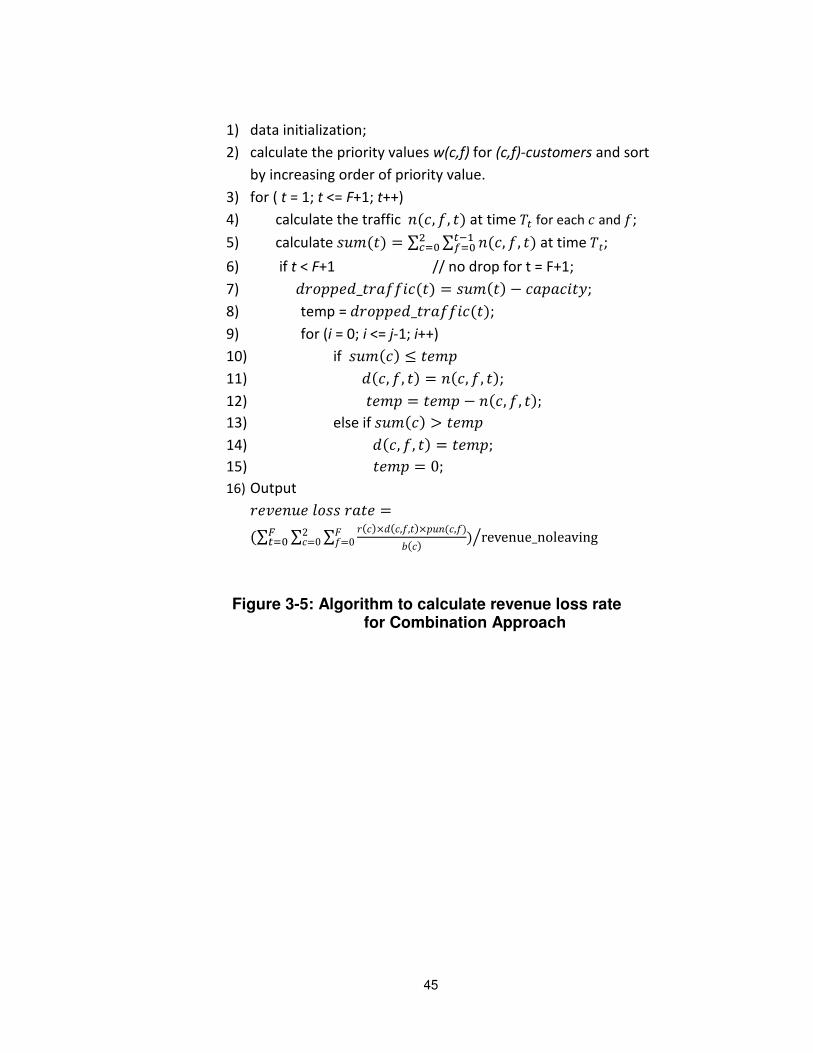
45


2) calculate the priority values w(c,f) for (c,f)-customers and sort

by increasing order of priority value.

3) for ( t = 1; t <= F+1; t++)

4) calculate the traffic ��, �, �� at time �� for each � and �;

5) calculate |�}�� ! ∑ ∑ ��, �, ��,�iW�UVW� at time ��; 6) if t < F+1 // no drop for t = F+1;

7) � ��Z�_� ��Q�� ! |�}�� Q�#;

8) temp = � ��Z�_� ��Q��; 9) for (i = 0; i <= j-1; i++)

10) if |�}�� ] �Z}�

11) ��, �, �� ! ��, �, ��; 12) �Z}� ! �Z}� � ��, �, ��; 13) else if |�}�� d �Z}�

14) ��, �, �� ! �Z}�; 15) �Z}� ! 0; 16) Output Z_Z�Z Y�|| ��Z !�∑ ∑ ∑ ��&��,�,��&��,�� revenue_noleaving��!02�!0��W�

Figure 3-5: Algorithm to calculate revenue loss rate for Combination Approach

46

4. EXPERIMENTS AND PERFORMANCE COMPARISON

There are five predictor variables in our models: the number of failures in

one experimental period (F), the probability that a ��-customer is watching a

VOD program (��), � Q�YZ � ��Q�, revenue-ratio between ��-customers, and

the probability that a ��, �� -customer unsubscribes from the VOD service

( ��, �� . To obtain the maximum information from our experiments, we

conduct a 2k factorial design and a full factorial design [43] to efficiently evaluate

the effects of the five predictor variables and compare the performance of all our

models. The findings from our experimental designs are informative to service

providers. The software Lingo was used as the linear program solver for our LP

model. Simulations for all our on-line models were coded in the C++

programming language; the simulations in [3] were also reproduced so that we

can compare the performances of our approaches with those of their

approaches. Results from the 2k factorial experiments show that the number of

failures F and the probability ��, �� are the two most important predictor

variables for the revenue loss rate. Findings from the full factorial experiments

suggest that the linear programming model for Optimal Approach always

outperforms other models and in this model, revenue loss can even be minimized

to 0 in some cases. Among all of our on-line approaches, the performance of

Revenue Approach is always the worst. Failure and Combination approaches

perform as well as Optimal Approach in some cases and can even reduce the

47

revenue loss to zero at times. Although Combination Approach is designed to

identify the locally optimal solution at each time that a failure occurs, Bandwidth

Approach can achieve better performance than Combination Approach in some

cases. By introducing bandwidth statistics, our approaches perform better than

the approaches in [3] in our simulations. Specific case studies are also

conducted,

(1) to examine the influence of α, the tuneable factor in Combination

Approach, on customers’ priority rankings;

(2) to determine why Optimal Approach always performs better than

Combination Approach;

(3) to explain why and how the variable, ��, the probability that a ��-customer is watching a VOD program, is critical in helping to minimize

the revenue loss to 0, even if it was not identified as a major predictor

variable in the 2k factorial experiment;

(4) to simulate three situations in which varying numbers of new

customers arrive in each interval between two adjacent failures in

order to learn how randomly occurring failures may affect revenue loss.

4.1 Background Description for Experiments

The experiments are designed based on the assumptions introduced in

Section 3.2.2. We assume that the VOD service is provided in a simple point-to-

point DWDM ring network with one centralized server and one distribution node,

as shown in Figure 3-1. The fixed capacity on each link is 10Gb. There are three

48

different types of VOD programs, standard-definition (SD) VOD, DVD-quality

video streams and high-definition (HD) VOD programs, which, on average, use

bandwidths of 3.75Mbps, 9.8Mbps, and 19Mbps, respectively [42]. We only study

the cases where the capacity of the surviving link cannot accommodate all the

traffic in peak traffic time when a failure happens. Therefore, we assume that the

total amount of the initial traffic is 10Gb, which is evenly distributed to the two

point-to-point links so that half of the bandwidth of each link is occupied.

Moreover, there are always new customers joining the network to ensure that the

total traffic always exceeds the capacity of one link. The total number of failures

for each experimental period determines the amount of traffic caused by new

customers at each time �� so that the total traffic at the end time �� equals the

full capacity of both links if no customers leave. For example, if there are 4

failures, the traffic for newly joined customers is 10Gb/5 = 2Gb at each interval

between two adjacent failures; and the total traffic at the end time �� is 20Gb

without any customer unsubscriptions. Performance results are calculated as the

percentage of revenue loss.

4.1.1 Determination of values for predictor variables

We are very careful about the determination of values for all the predictor

variables because without realistic value ranges, the findings on the impact of

each predictor variable and the performance of each approach would be of little

value. The values for the predictor variables were determined based on our more

realistic assumptions and we discarded some arbitrary value assumptions in [3].

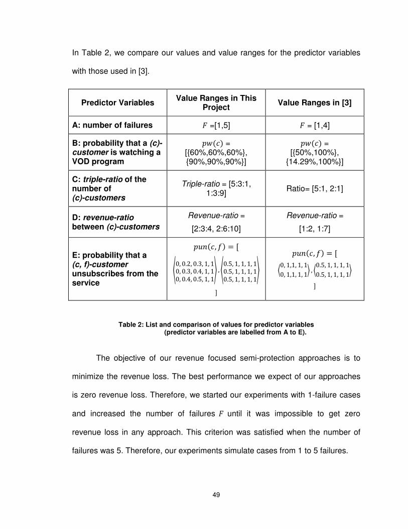
49

In Table 2, we compare our values and value ranges for the predictor variables

with those used in [3].

Table 2: List and comparison of values for predictor variables (predictor variables are labelled from A to E).

The objective of our revenue focused semi-protection approaches is to

minimize the revenue loss. The best performance we expect of our approaches

is zero revenue loss. Therefore, we started our experiments with 1-failure cases

and increased the number of failures � until it was impossible to get zero

revenue loss in any approach. This criterion was satisfied when the number of

failures was 5. Therefore, our experiments simulate cases from 1 to 5 failures.

Predictor Variables Value Ranges in This

Project Value Ranges in [3]

A: number of failures � =[1,5] � = [1,4]

B: probability that a (c)-customer is watching a VOD program

�� = [{60%,60%,60%}, {90%,90%,90%}]

�� = [{50%,100%},

{14.29%,100%}] C: triple-ratio of the number of (c)-customers

Triple-ratio = [5:3:1, 1:3:9]

Ratio= [5:1, 2:1]

D: revenue-ratio between (c)-customers

Revenue-ratio =

[2:3:4, 2:6:10]

Revenue-ratio =

[1:2, 1:7]

E: probability that a (c, f)-customer unsubscribes from the service

��, �� ! S �0, 0.2, 0.3, 1, 10, 0.3, 0.4, 1, 10, 0.4, 0.5, 1, 1� , �

0.5, 1, 1, 1, 10.5, 1, 1, 1, 10.5, 1, 1, 1, 1� T

��, �� ! S �0, 1,1, 1, 10, 1,1, 1, 1� , �0.5, 1, 1, 1, 10.5, 1, 1, 1, 1� T

50

A recent survey (2007) by Nielsen Media Research showed that more

than 50% of households are watching TV programs during the television

watching prime time (e.g. 8pm-11pm in U.S.). Typically, the peak traffic time is

during the prime time and the network bandwidth is probably enough to support

full protection for all traffic during off-peak times. We only examine the situation

that one surviving link cannot accommodate all traffic when a failure happens

during the peak traffic time. Thus we assume that the range of �� is from 60%

to 90%. Only two cases were considered in [3]: in the first case, higher revenue

customers watch the VOD programs with probability 100% and lower revenue

customers watch with probability 50% (one day out of two); in the second case,

higher revenue customers watch the VOD programs with probability 100% and

lower revenue customers watch with probability 14.29% (one day per week). We

assume that the probability for all customers watching VOD programs is the

same during peak traffic time. Hence we assigned each customer the same

probability �� in our experiments and the probability is always a value in the

range from 60% to 90%.

In [3], the ratio of the numbers of two different classes of customers is in

the range 5:1 to 2:1. Similar to the left end of their range: 5:1, our triple-ratios

start at 5:3:1. To decide on the right end of the range of our triple-ratios, we

referred to the findings of some recent surveys, which revealed that nowadays

almost all replacement TV sets purchased are HDTV sets. We expect that in the

near future, most customers will be watching HDTV programs and thus we set

the right end of the range to be 1:3:9 for our experiments. Comparing the pricing

51

of current VOD services, which ranges from $4 to $13 per VOD order or from $20

to $100 subscription fees per month, we set the range for the values of revenue-

ratios to be from 2:3:4 to 2:6:10.

In our experiments, we enlarged the value ranges for the predictor

variable ��, ��, using a probability matrix to accommodate the possibility that

customers may show more tolerance of network interruptions than the low

tolerance (i.e., all customers will unsubscribe after experiencing the second

interruption) assumed in [3]. Our values of ��, �� also ensure that the

probabilities for different (c)-customers reflect our assumption that ��, �� indicates customers’ expectations of the reliability of network services. The

higher revenue customers may have higher expectations, and thus higher

probabilities to unsubscribe from the service if they encounter service

interruptions. In addition, we also studied the impact of two intermediate values,

��, �� ! ��,�.�,�,�,��,�.�,�,�,��,�.0,�,�,�� and ��, �� ! ��.U,�.�,�,�,��.l,�.�,�,�,��.�,�.0,�,�,�� , on the performance of our

models in the full factorial experimental design.

4.2 2k Experimental Design

In order to identify the impact of the five predictor variables, a 2k

experimental design was adopted to analyze the effects of the predictor variables

and their interactions on revenue loss rate, using two levels of predictor variables:

low and high. The 2k experimental design reduces the total number of

experiments needed for further analysis and ranks the importance of each

52

predictor variable in an efficient way, based on the proportion of the total

variation attributed to each variable.

Following the 2k experimental design procedures[43], with H ! 5 (the

number of predictor variables), we first set the two levels of each predictor

variable, with the low level indicated by the sign, -1, and the high level indicated

by the sign, 1, as shown in Table 3.

Table 3: Levels and signs for the 5 predictor variables.

After we assigned levels and signs to the predictor variables, we

conducted the experiments and used the experimental results from each

approach to form a 32-equation set with 25 variables. The variables in the 32-

equation set include all possible combinations of the 5 predictor variables so that

all interactions between these predictor variables are examined. We labelled the

Impact Factors Low Level

(sign: -1)

High Level

(sign: 1) Number Notation

A � 1 5

B �� {60%,60%,60%} {90%,90%,90%}

C � Q�YZ � ��Q� 5:3:1 1:3:9

D Z_Z�Z ��Q� 2:3:4 2:6:10

E ��, �� 0, 0.2, 0.3, 1, 10, 0.3, 0.4, 1, 10, 0.4, 0.5, 1, 1� �0.5, 1, 1, 1, 10.5, 1, 1, 1, 10.5, 1, 1, 1, 1�

53

5 predictor variables from A to E as shown in Table 3. Thus, the impact variable

AB stands for the interaction between A and B, the impact variable ABE stands

for the interaction among A, B and E, and so on. We used the software Lingo to

solve the 32-equation set and the results, the proportion of the total variation

explained by each impact variable, are shown in Table 4. The order of the impact

of all the impact variables is determined by the proportion of the total variation

accounted for by each variable. As we can see from Table 4, the effects of all the

second order and higher interactions are negligible because the total variation

explained by these interactions is less than 1%, much smaller than that

accounted for by the first order and primary impact variables, which are 15.92%

and 83.75% respectively. The primary order variables A (the number of failures)

and E (the probability of a customer leaving), which explained more than 93% of

the total variation at the primary order in all six approaches, are identified as two

major predictor variables. For example, for Optimal Approach, the proportion of

explained variation by A and E is 96.12% of the total primary variation 83.75%;

for Bandwidth Approach, it is 93.31%. In comparison, the effects of variable B

(the probability of a customer watching VOD), C (the triple-ratio) and D (the

revenue-ratio) are relatively minor and thus were not considered in our full

factorial experimental design. It is worth noting that the impact of the five

predictor variables on revenue loss rate varies by approach. For example,

variable E is more influential than variable A in Optimal, Failure, and Combination

approaches, but is less important than variable A in other approaches; the

revenue-ratio has a minor effect in Revenue Approach, but no impact at all in

54

Failure and Random approaches. At the first order, the most significant

interaction is AE, which accounted for 88% (14% out of 15.92%), 83%, 44%,

49%, 90%, and 85% of the total variation explained by all the 10 interaction first

order variables in the six approaches respectively. The second most significant

interaction is AB, which, at most, accounted for 22% of the total variation in

Revenue Approach. Among all the approaches, the biggest variation explained

by AE is 14%, whereas for AB, it is only 1.33%. Therefore, we only considered A

and E as important predictor variables in our full factorial experimental design.

Factors Optimal

Approach

Random

Approach

Revenue

Approach

Bandwidth

Approach

Failure

Approach

Comb.

Approach Primary

Effects 83.75% 91.77% 93.09% 92.89% 86.51% 85.05%

A 22.07% 45.10% 55.41% 56.86% 25.72% 25.75%

B 2.45% 3.35% 3.80% 3.59% 3.78% 3.67%

C 0.35% 0.05% 0.35% 0.18% 0.01% 0.40%

D 0.45% 0.00% 2.07% 1.35% 0.00% 0.33%

E 58.43% 43.27% 31.46% 30.91% 57.00% 54.90%

First

order 15.92% 8.07% 6.01% 6.37% 13.17% 14.40%

AB 0.62% 1.06% 1.33% 1.29% 1.26% 1.28%

AC 0.06% 0.05% 0.18% 0.01% 0.01% 0.08%

AD 0.09% 0.00% 0.84% 0.60% 0.00% 0.04%

AE 14.00% 6.68% 2.65% 3.10% 11.79% 12.24%

BC 0.03% 0.00% 0.02% 0.03% 0.01% 0.05%

BD 0.01% 0.00% 0.04% 0.03% 0.00% 0.00%

BE 0.37% 0.23% 0.02% 0.08% 0.09% 0.12%

CD 0.14% 0.00% 0.59% 0.60% 0.00% 0.09%

CE 0.17% 0.05% 0.07% 0.39% 0.01% 0.07%

DE 0.43% 0.00% 0.27% 0.24% 0.00% 0.43%

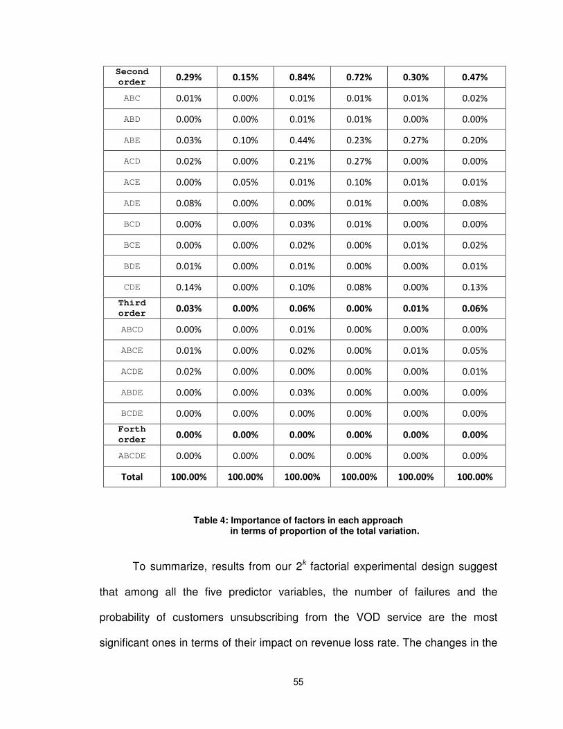
55

Table 4: Importance of factors in each approach in terms of proportion of the total variation.

To summarize, results from our 2k factorial experimental design suggest

that among all the five predictor variables, the number of failures and the

probability of customers unsubscribing from the VOD service are the most

significant ones in terms of their impact on revenue loss rate. The changes in the

Second

order 0.29% 0.15% 0.84% 0.72% 0.30% 0.47%

ABC 0.01% 0.00% 0.01% 0.01% 0.01% 0.02%

ABD 0.00% 0.00% 0.01% 0.01% 0.00% 0.00%

ABE 0.03% 0.10% 0.44% 0.23% 0.27% 0.20%

ACD 0.02% 0.00% 0.21% 0.27% 0.00% 0.00%

ACE 0.00% 0.05% 0.01% 0.10% 0.01% 0.01%

ADE 0.08% 0.00% 0.00% 0.01% 0.00% 0.08%

BCD 0.00% 0.00% 0.03% 0.01% 0.00% 0.00%

BCE 0.00% 0.00% 0.02% 0.00% 0.01% 0.02%

BDE 0.01% 0.00% 0.01% 0.00% 0.00% 0.01%

CDE 0.14% 0.00% 0.10% 0.08% 0.00% 0.13%

Third

order 0.03% 0.00% 0.06% 0.00% 0.01% 0.06%

ABCD 0.00% 0.00% 0.01% 0.00% 0.00% 0.00%

ABCE 0.01% 0.00% 0.02% 0.00% 0.01% 0.05%

ACDE 0.02% 0.00% 0.00% 0.00% 0.00% 0.01%

ABDE 0.00% 0.00% 0.03% 0.00% 0.00% 0.00%

BCDE 0.00% 0.00% 0.00% 0.00% 0.00% 0.00%

Forth

order 0.00% 0.00% 0.00% 0.00% 0.00% 0.00%

ABCDE 0.00% 0.00% 0.00% 0.00% 0.00% 0.00%

Total 100.00% 100.00% 100.00% 100.00% 100.00% 100.00%

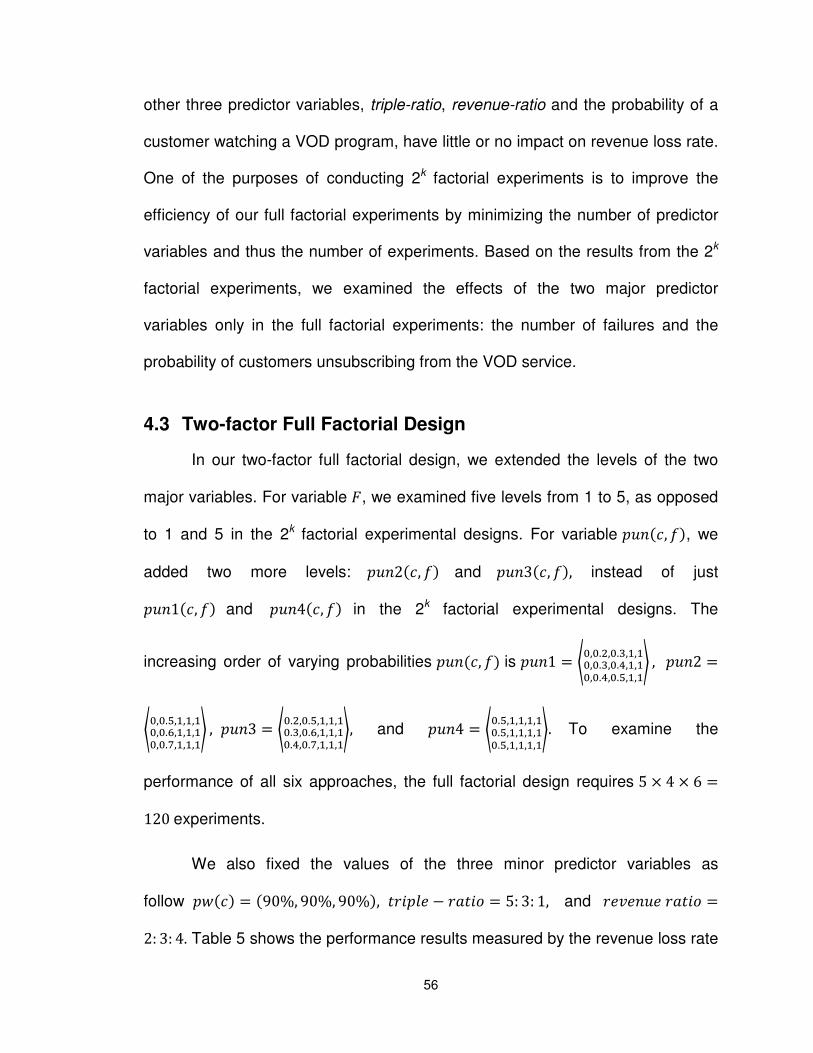
56

other three predictor variables, triple-ratio, revenue-ratio and the probability of a

customer watching a VOD program, have little or no impact on revenue loss rate.

One of the purposes of conducting 2k factorial experiments is to improve the

efficiency of our full factorial experiments by minimizing the number of predictor

variables and thus the number of experiments. Based on the results from the 2k

factorial experiments, we examined the effects of the two major predictor

variables only in the full factorial experiments: the number of failures and the

probability of customers unsubscribing from the VOD service.

4.3 Two-factor Full Factorial Design

In our two-factor full factorial design, we extended the levels of the two

major variables. For variable �, we examined five levels from 1 to 5, as opposed

to 1 and 5 in the 2k factorial experimental designs. For variable ��, ��, we

added two more levels: ��2��, �� and ��3��, ��, instead of just

��1��, �� and ��4��, �� in the 2k factorial experimental designs. The

increasing order of varying probabilities ��, �� is ��1 ! ��,�.U,�.l,�,��,�.l,�.�,�,��,�.�,�.�,�,�� , ��2 !��,�.�,�,�,��,�.�,�,�,��,�.0,�,�,�� , ��3 ! ��.U,�.�,�,�,��.l,�.�,�,�,��.�,�.0,�,�,��, and ��4 ! ��.�,�,�,�,��.�,�,�,�,��.�,�,�,�,��. To examine the

performance of all six approaches, the full factorial design requires 5 & 4 & 6 !120 experiments.

We also fixed the values of the three minor predictor variables as

follow �� ! �90%, 90%, 90%�, � Q�YZ � ��Q� ! 5: 3: 1, and Z_Z�Z ��Q� !2: 3: 4. Table 5 shows the performance results measured by the revenue loss rate

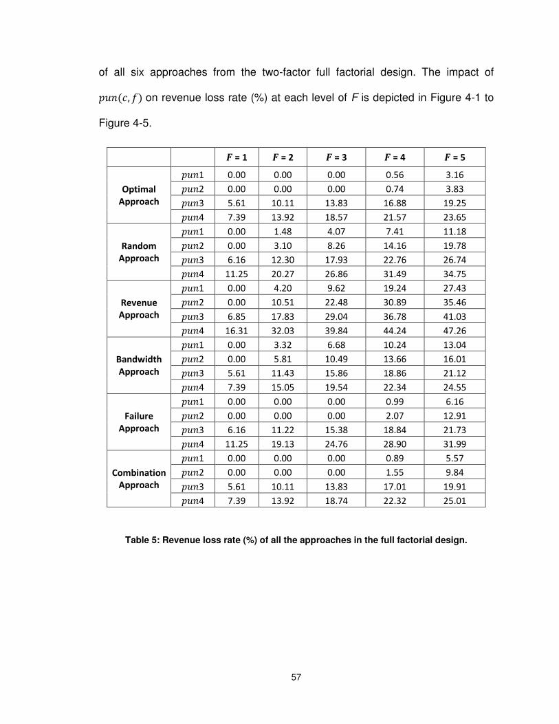
57

of all six approaches from the two-factor full factorial design. The impact of

��, �� on revenue loss rate (%) at each level of F is depicted in Figure 4-1 to

Figure 4-5.

¢ = 1 ¢ = 2 ¢ = 3 ¢ = 4 ¢ = 5

Optimal

Approach

��1 0.00 0.00 0.00 0.56 3.16 ��2 0.00 0.00 0.00 0.74 3.83 ��3 5.61 10.11 13.83 16.88 19.25 ��4 7.39 13.92 18.57 21.57 23.65

Random

Approach

��1 0.00 1.48 4.07 7.41 11.18 ��2 0.00 3.10 8.26 14.16 19.78 ��3 6.16 12.30 17.93 22.76 26.74 ��4 11.25 20.27 26.86 31.49 34.75

Revenue

Approach

��1 0.00 4.20 9.62 19.24 27.43 ��2 0.00 10.51 22.48 30.89 35.46 ��3 6.85 17.83 29.04 36.78 41.03 ��4 16.31 32.03 39.84 44.24 47.26

Bandwidth

Approach

��1 0.00 3.32 6.68 10.24 13.04 ��2 0.00 5.81 10.49 13.66 16.01 ��3 5.61 11.43 15.86 18.86 21.12 ��4 7.39 15.05 19.54 22.34 24.55

Failure

Approach

��1 0.00 0.00 0.00 0.99 6.16 ��2 0.00 0.00 0.00 2.07 12.91 ��3 6.16 11.22 15.38 18.84 21.73 ��4 11.25 19.13 24.76 28.90 31.99

Combination

Approach

��1 0.00 0.00 0.00 0.89 5.57 ��2 0.00 0.00 0.00 1.55 9.84 ��3 5.61 10.11 13.83 17.01 19.91 ��4 7.39 13.92 18.74 22.32 25.01

Table 5: Revenue loss rate (%) of all the approaches in the full factorial design.

58

Figure 4-1: Revenue loss rate (%) when F = 1.


0.00

2.00

4.00

6.00

8.00

10.00

12.00

14.00

16.00

18.00

pun1 pun2 pun3 pun4

Re

ve

nu

e lo

ss r

ate

(%

)

pun(c, f)

Optimal

Random

Revenue

Bandwidth

FailureBand.Comb.Optimal

FailureRandom

0.00

5.00

10.00

15.00

20.00

25.00

30.00

35.00

pun1 pun2 pun3 pun4

Re

ve

nu

e lo

ss r

ate

(%

)

pun(c,f)

Optimal

Random

Revenue

Bandwidt

hComb.Optimal

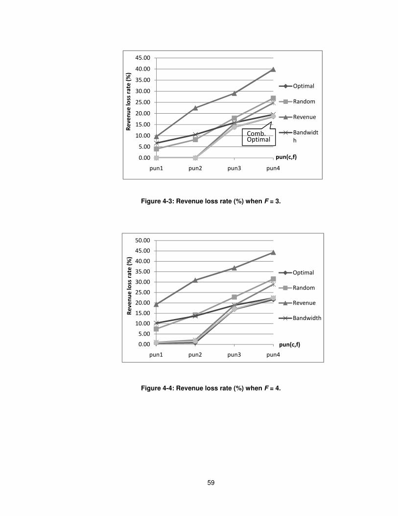
59



0.00

5.00

10.00

15.00

20.00

25.00

30.00

35.00

40.00

45.00

pun1 pun2 pun3 pun4

Re

ve

nu

e lo

ss r

ate

(%

)

pun(c,f)

Optimal

Random

Revenue

Bandwidt

hComb.Optimal

0.00

5.00

10.00

15.00

20.00

25.00

30.00

35.00

40.00

45.00

50.00

pun1 pun2 pun3 pun4

Re

ve

nu

e lo

ss r

ate

(%

)

pun(c,f)

Optimal

Random

Revenue

Bandwidth

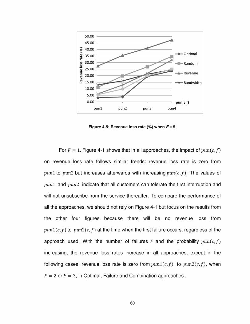
60


For � ! 1, Figure 4-1 shows that in all approaches, the impact of ��, �� on revenue loss rate follows similar trends: revenue loss rate is zero from

��1 to ��2 but increases afterwards with increasing ��, ��. The values of

��1 and ��2 indicate that all customers can tolerate the first interruption and

will not unsubscribe from the service thereafter. To compare the performance of

all the approaches, we should not rely on Figure 4-1 but focus on the results from

the other four figures because there will be no revenue loss from

��1��, �� to ��2��, �� at the time when the first failure occurs, regardless of the

approach used. With the number of failures � and the probability ��, �� increasing, the revenue loss rates increase in all approaches, except in the

following cases: revenue loss rate is zero from ��1��, �� to ��2��, ��, when

� ! 2 or � ! 3, in Optimal, Failure and Combination approaches .

0.00

5.00

10.00

15.00

20.00

25.00

30.00

35.00

40.00

45.00

50.00

pun1 pun2 pun3 pun4

Re

ve

nu

e lo

ss r

ate

(%

)

pun(c,f)

Optimal

Random

Revenue

Bandwidth

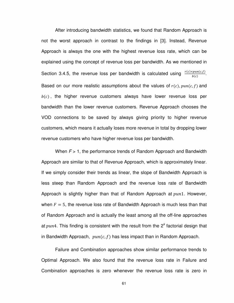
61

After introducing bandwidth statistics, we found that Random Approach is

not the worst approach in contrast to the findings in [3]. Instead, Revenue

Approach is always the one with the highest revenue loss rate, which can be

explained using the concept of revenue loss per bandwidth. As we mentioned in

Section 3.4.5, the revenue loss per bandwidth is calculated using 6�V�&q89�V,i�7�V� .

Based on our more realistic assumptions about the values of ��, ��, �� and

�� , the higher revenue customers always have lower revenue loss per

bandwidth than the lower revenue customers. Revenue Approach chooses the

VOD connections to be saved by always giving priority to higher revenue

customers, which means it actually loses more revenue in total by dropping lower

revenue customers who have higher revenue loss per bandwidth.

When F > 1, the performance trends of Random Approach and Bandwidth

Approach are similar to that of Revenue Approach, which is approximately linear.

If we simply consider their trends as linear, the slope of Bandwidth Approach is

less steep than Random Approach and the revenue loss rate of Bandwidth

Approach is slightly higher than that of Random Approach at ��1. However,

when � ! 5, the revenue loss rate of Bandwidth Approach is much less than that

of Random Approach and is actually the least among all the off-line approaches

at ��4. This finding is consistent with the result from the 2k factorial design that

in Bandwidth Approach, ��, �� has less impact than in Random Approach.

Failure and Combination approaches show similar performance trends to

Optimal Approach. We also found that the revenue loss rate in Failure and

Combination approaches is zero whenever the revenue loss rate is zero in

62

Optimal Approach. All three approaches have much lower revenue loss rate than

the other approaches when � r 5 and the probability ��, �� is low, such as

��, �� ! ��1 or ��2. This finding is understandable because both Failure

and Combination approaches always first drop the connections of those

customers who are less likely to unsubscribe from the service if their connections

are dropped. Apparently, this is how Failure Approach determines the

connections to be dropped. Combination Approach calculates priority values

using ��, ��, and assigns lower priority to customers who have experienced

fewer interruptions, especially those customers whose probability of

unsubscribing is zero. We can also see in the five figures that there are sudden

increases in the revenue loss rate in all three approaches when ��, �� changes from ��2 to ��3 and their performances get close to the

performances of the other approaches. This is caused by the fact that none of

the three approaches can benefit from customers with low probabilities to

unsubscribe at ��3 and ��4, where there are few customers who can tolerate

even the first interruption.

4.4 Result Comparison with Previous Research

We compared the performance results of our approaches with the results

in [3] and found that our approaches achieve better performance in terms of

minimizing the revenue loss after introducing bandwidth statistics and using more

realistic values for predictor variables.

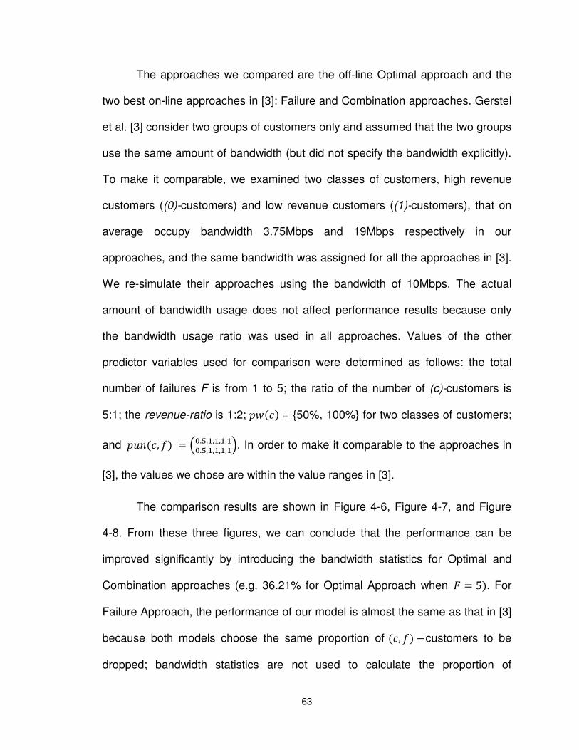
63

The approaches we compared are the off-line Optimal approach and the

two best on-line approaches in [3]: Failure and Combination approaches. Gerstel

et al. [3] consider two groups of customers only and assumed that the two groups

use the same amount of bandwidth (but did not specify the bandwidth explicitly).

To make it comparable, we examined two classes of customers, high revenue

customers ((0)-customers) and low revenue customers ((1)-customers), that on

average occupy bandwidth 3.75Mbps and 19Mbps respectively in our

approaches, and the same bandwidth was assigned for all the approaches in [3].

We re-simulate their approaches using the bandwidth of 10Mbps. The actual

amount of bandwidth usage does not affect performance results because only

the bandwidth usage ratio was used in all approaches. Values of the other

predictor variables used for comparison were determined as follows: the total

number of failures F is from 1 to 5; the ratio of the number of (c)-customers is

5:1; the revenue-ratio is 1:2; �� = {50%, 100%} for two classes of customers;

and ��, �� ! £�.�,�,�,�,��.�,�,�,�,�¤. In order to make it comparable to the approaches in

[3], the values we chose are within the value ranges in [3].

The comparison results are shown in Figure 4-6, Figure 4-7, and Figure

4-8. From these three figures, we can conclude that the performance can be

improved significantly by introducing the bandwidth statistics for Optimal and

Combination approaches (e.g. 36.21% for Optimal Approach when � ! 5�. For

Failure Approach, the performance of our model is almost the same as that in [3]

because both models choose the same proportion of ��, �� customers to be

dropped; bandwidth statistics are not used to calculate the proportion of

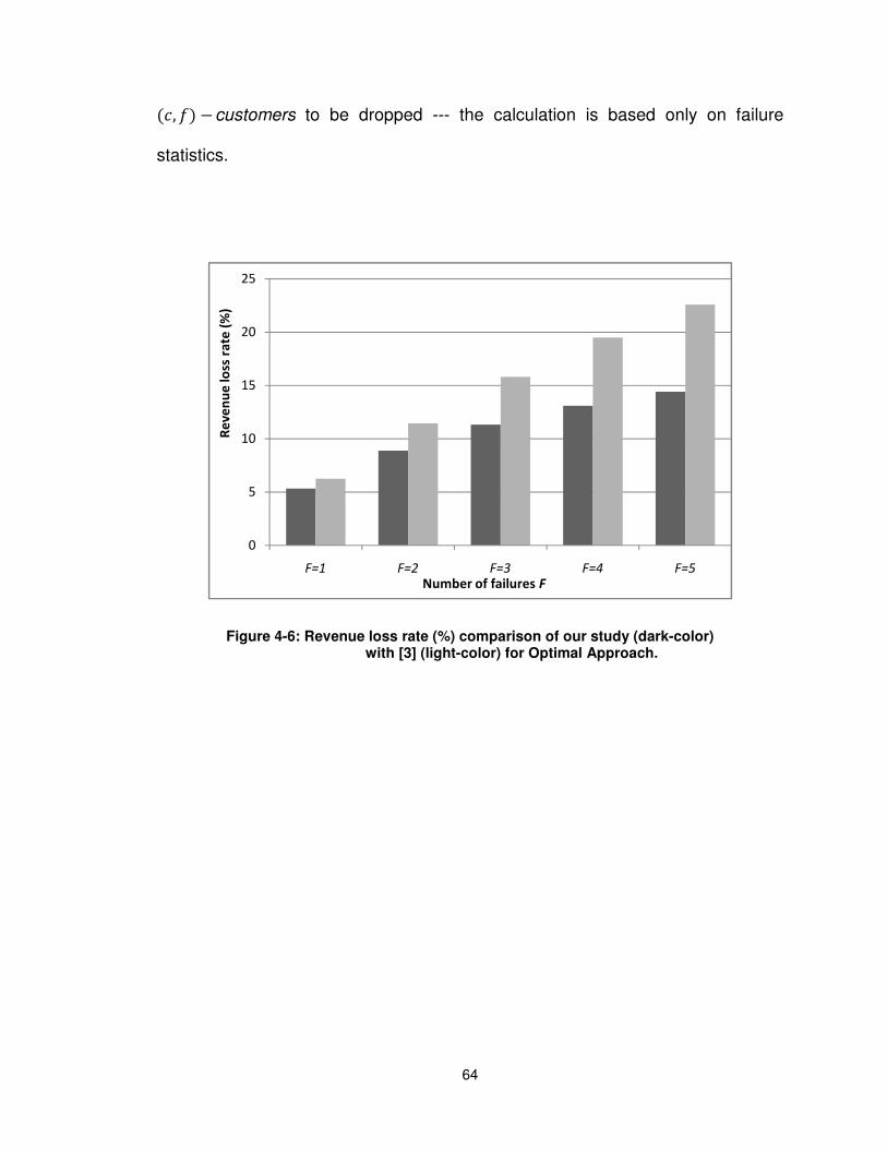
64

��, �� customers to be dropped --- the calculation is based only on failure

statistics.

Figure 4-6: Revenue loss rate (%) comparison of our study (dark-color) with [3] (light-color) for Optimal Approach.

0

5

10

15

20

25

F=1 F=2 F=3 F=4 F=5

Re

ve

nu

e lo

ss r

ate

(%

)

Number of failures F

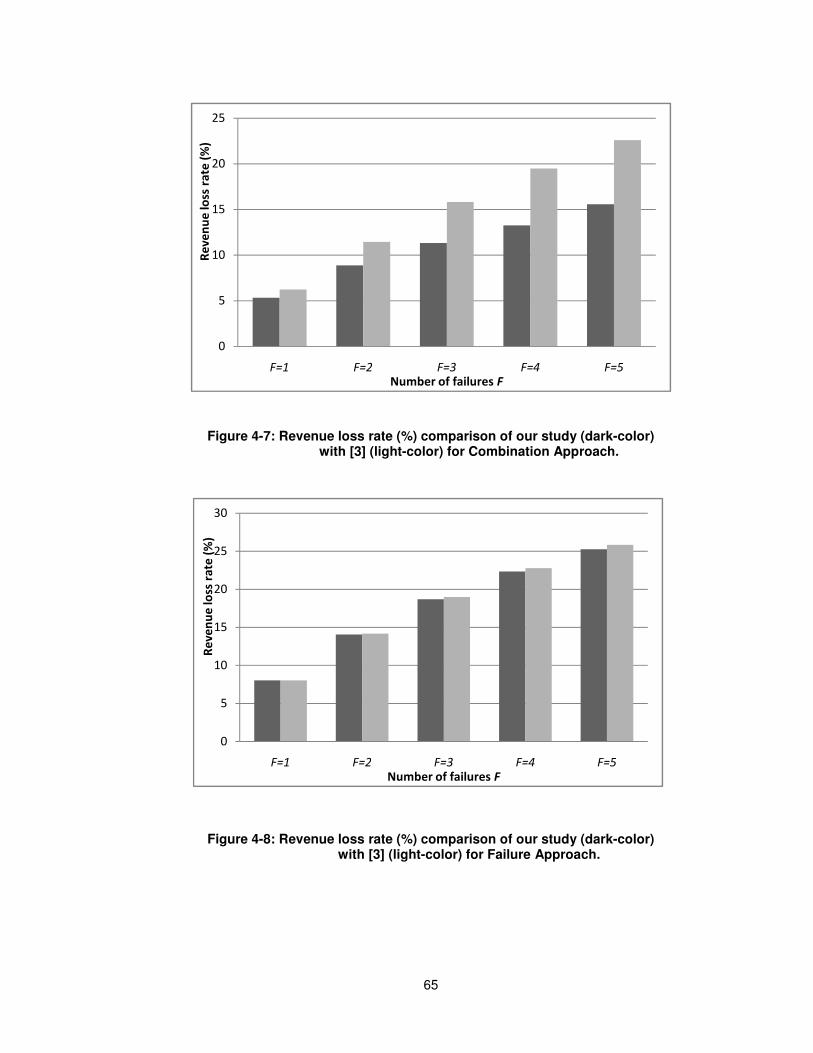
65

Figure 4-7: Revenue loss rate (%) comparison of our study (dark-color) with [3] (light-color) for Combination Approach.

Figure 4-8: Revenue loss rate (%) comparison of our study (dark-color) with [3] (light-color) for Failure Approach.

0

5

10

15

20

25

F=1 F=2 F=3 F=4 F=5

Re

ve

nu

e lo

ss r

ate

(%

)


0

5

10

15

20

25

30

F=1 F=2 F=3 F=4 F=5

Re

ve

nu

e lo

ss r

ate

(%

)


66

4.5 Observations

We evaluated the impact of the five predictor variables using the 2k

factorial experimental design and compared the performance of all six

approaches using the full factorial experimental design. In this section, we

summarize our observations.

I. Results from our study suggest that the two predictor variables ---

the number of failures F and the probability of customers

unsubscribing from the service ��, �� --- and their interactions

have significant effects on the performance of all the approaches.

II. Optimal Approach, as the only off-line approach, outperforms all

the on-line approaches in all cases.

III. Combination Approach achieves the best overall performance

among the on-line approaches by using locally optimal solutions.

IV. In most cases, Failure Approach performs as well as Combination

Approach because both approaches always first drop the

connections of those customers who are less likely to unsubscribe

from the service if their connections are dropped.

V. Optimal, Combination and Failure approaches can keep revenue

loss at zero in the situations when all customers can tolerate at

least one interruption. Whenever Optimal Approach can achieve

zero revenue loss, so can Combination and Failure approaches.

67

VI. Our results are quite different from the findings in [3]. In our study,

Random Approach is not the worst approach. Instead, Revenue

Approach performs the worst because it fails to optimize the

selection of connections to be dropped. For example, between

(0,3,5)-customers and (2,0,5)-customers at time �� , Revenue

Approach chooses to drop the connections of (0,3,5)-customers

who have lower revenue contributions but higher probability to

unsubscribe, when in fact dropping the connections of (2,0,5)-

customers leads to no revenue loss.

VII. After adding bandwidth statistics, Bandwidth Approach proposed in

this project can achieve the best performance of all on-line

approaches.

VIII. We extended the five approaches used in [3] by introducing

bandwidth statistics. Compared with the approaches in [3], our

approaches achieve better performance by further reducing the

revenue loss rate by as much as 36%.

4.6 Specific Case Studies

4.6.1 Case 1: Impact of factor ¥ in Combination Approach

In Section 3.4.5, we discussed that the different groups of ��, ��-customers

may be assigned the same priorities in Combination Approach. To prevent this

kind of situation, the tuneable factor α is used to take into account the priority of

��, � % 1�-customers to slightly adjust the priority of ��, ��-customers; ��, � % 1�-

68

customers are the ��, ��-customers whose connections are dropped by the f+1st

interruption but they keep subscribing to the service. The side effects of α are:

the calculation of priority values of ��, �� -customers are based on the

consideration of the impact of future failures even when these future failures do

not actually occur; α can radically change the priority ranking of ��, ��-customers

in situations when ��-customers are not assigned the same priorities without the

adjustment of α. These side effects of α may influence Combination Approach in

such a way that it cannot achieve the locally optimal solution at each time �� using the order of priorities ranked by revenue loss per bandwidth. In this section,

we analyze the effects of α on the performance of Combination Approach to

provide guidelines on how to properly determine the value of α so that the side

effects of α can be avoided. With increasing α, the impact of the priorities of

��, � % 1� �customers on the priorities of ��, �� customers is also increasing in

Combination Approach and leads to a reordering of the priority ranks of all

customers, which may prevent Combination Approach from achieving the least

revenue loss per bandwidth at each time�� . We simulated this reordering of

priority ranks by changing the value of α in two experiments, Experiment 1 and

Experiment 2. The impact of α on the performance of Combination Approach is

shown in Figure 4-9. The fixed values that we used for the other variables in the

two experiments are shown in Table 6.

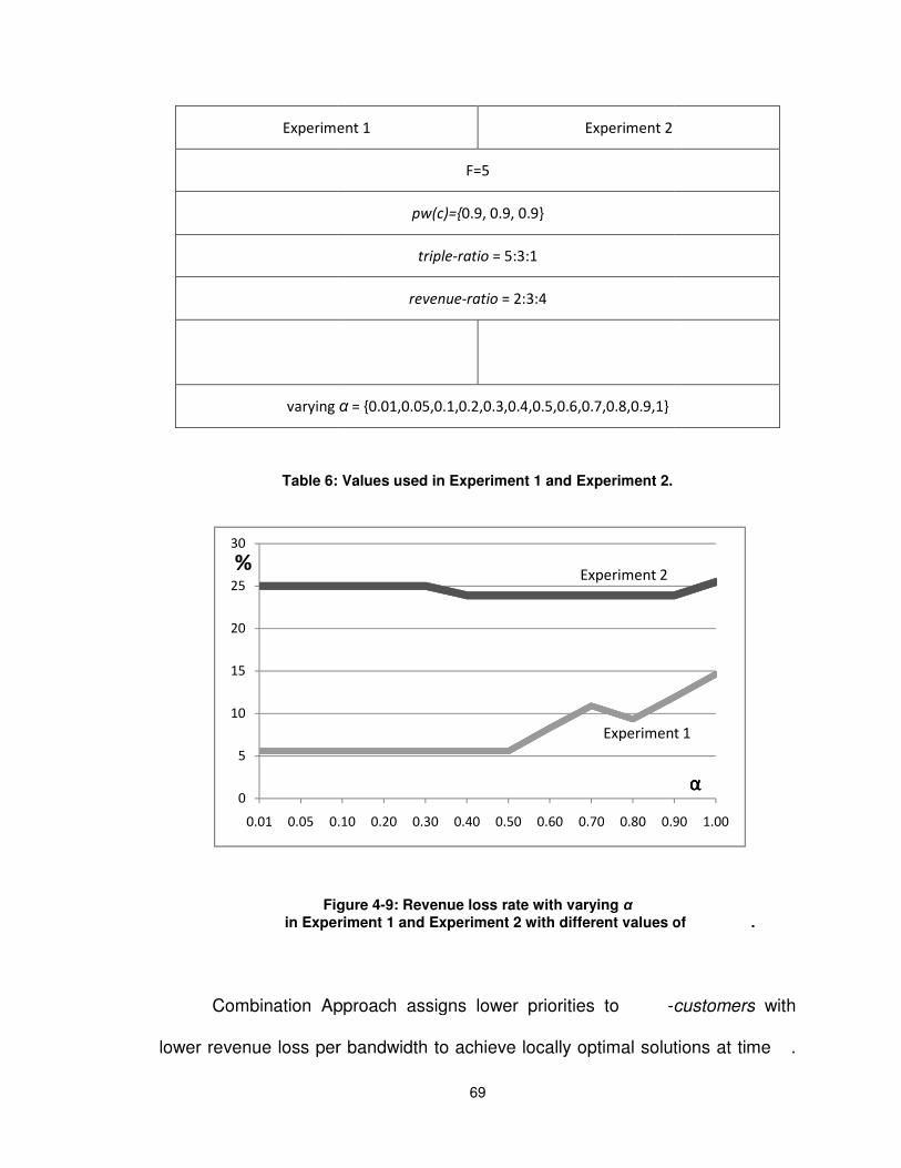
Experiment

varying

Table 6: Values used in

Figure in Experiment

Combination Approach assigns

lower revenue loss per bandwidth to achieve local

0

5

10

15

20

25

30

0.01 0.05 0.10

%

69

Experiment 1 Experiment 2

F=5

pw(c)={0.9, 0.9, 0.9}

triple-ratio = 5:3:1

revenue-ratio = 2:3:4

varying α = {0.01,0.05,0.1,0.2,0.3,0.4,0.5,0.6,0.7,0.8,0.9,1}

: Values used in Experiment 1 and Experiment 2.

Figure 4-9: Revenue loss rate with varying α Experiment 1 and Experiment 2 with different values of

Combination Approach assigns lower priorities to -customers

revenue loss per bandwidth to achieve locally optimal solutions at time

0.10 0.20 0.30 0.40 0.50 0.60 0.70 0.80 0.90

Experiment 1

Experiment 2

of .

customers with

optimal solutions at time .

0.90 1.00

ααα

Experiment 1

70

As shown in Figure 4-9, there are fluctuations in revenue loss rate as α varies in

both Experiment 1 and Experiment 2. Each turning point in the figure indicates

priority rank being reordered by changed α. When α is very low, for example,

when 1 r 0.3 in Experiment 2 and 1 r 0.5 in Experiment 1, the priority values of

��, ��-customers are mainly determined by revenue loss per bandwidth. When

1 d 0.3 in Experiment 2 and 1 d 0.5 in Experiment 1, the priority values and thus

the order of priority of ��, ��-customers have begun to be influenced by α, and do

not reflect the order of priority determined solely by revenue loss per bandwidth.

It is hard to expect a globally optimal solution from Combination Approach when

its local solution is not optimal. However, as shown in Figure 4-9, we did see

some improved global performance in Experiment 2. To figure out the reason for

the improved performance, we conducted Experiment 3 and Experiment 4 to

explain how α affects the revenue loss in Experiment 2 by reordering the priority

rank. Different values of α were examined in the two experiments: α = 0.01 in

Experiment 3 in order to show the priority rank without much influence of α, and α

= 0.5 in Experiment 4 in order to show the priority rank influenced by α. Values of

the other variables were the same as in Experiment 2. We show the priority ranks

of the different groups of ��, ��-customers from these two experiments in Table 7

and the dropped traffic (Mb) and the revenue loss ($) at the time each failure

happened in Table 8.

As we can see from Table 8, at the time when the first failure happens,

the same amount of traffic (1667Mb) is dropped in the two experiments, and the

same priority rank is used to choose (c,0)-customers to be dropped, which are

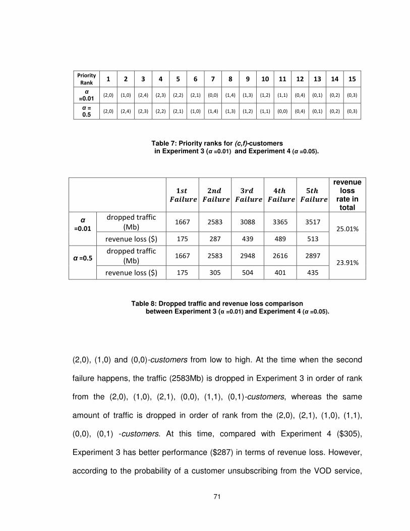
71

Priority

Rank 1 2 3 4 5 6 7 8 9 10 11 12 13 14 15

α =0.01

(2,0) (1,0) (2,4) (2,3) (2,2) (2,1) (0,0) (1,4) (1,3) (1,2) (1,1) (0,4) (0,1) (0,2) (0,3)

α = 0.5

(2,0) (2,4) (2,3) (2,2) (2,1) (1,0) (1,4) (1,3) (1,2) (1,1) (0,0) (0,4) (0,1) (0,2) (0,3)

Table 7: Priority ranks for (c,f)-customers in Experiment 3 (α =0.01) and Experiment 4 (α =0.05).

¦§¨ ¢¥©ª«¬

®¯° ¢¥©ª«¬

±¬° ¢¥©ª«¬

²¨³ ¢¥©ª«¬

´¨³ ¢¥©ª«¬

revenue loss

rate in total

α

=0.01

dropped traffic

(Mb) 1667 2583 3088 3365 3517

25.01%

revenue loss ($) 175 287 439 489 513

α =0.5

dropped traffic

(Mb) 1667 2583 2948 2616 2897

23.91%

revenue loss ($) 175 305 504 401 435

Table 8: Dropped traffic and revenue loss comparison between Experiment 3 (α =0.01) and Experiment 4 (α =0.05).

(2,0), (1,0) and (0,0)-customers from low to high. At the time when the second

failure happens, the traffic (2583Mb) is dropped in Experiment 3 in order of rank

from the (2,0), (1,0), (2,1), (0,0), (1,1), (0,1)-customers, whereas the same

amount of traffic is dropped in order of rank from the (2,0), (2,1), (1,0), (1,1),

(0,0), (0,1) -customers. At this time, compared with Experiment 4 ($305),

Experiment 3 has better performance ($287) in terms of revenue loss. However,

according to the probability of a customer unsubscribing from the VOD service,

72

the customers who occupy more traffic load than those in Experiment 3

unsubscribe from service in Experiment 4. Therefore, at the time when the 3rd

failure happens, less traffic (2948Mb) needs to be dropped in Experiment 4 than

in Experiment 3 (3088Mb). The same reason explains why less traffic (2616Mb,

and 2897Mb) needs to be dropped in Experiment 4, which, in turn, explains why

there is less revenue loss in Experiment 4 ($401 and $435) than in Experiment 3

($489 and $513), at the times when the 4th and 5th failures happen. This can also

help us to understand why at the end time �� , the total revenue loss rate is

smaller in Experiment 4 (23.91%) than in Experiment 3 (25.01%).

It is worth pointing out that when α = 1, equation II in Section 3.4.5 can be

simplified to ��, �� ! 6�V�7�V� & ��, �� % 6�V�7�V� & e1 � ��, ��f ! 6�V�7�V� . Therefore,

the priority values are constant for �� -customers regardless of the failure

statistics � . In this case, Combination Approach selects connections to be

dropped randomly.

Based on the above observations, we recommend that the values of α

should be small enough to avoid the unwanted side effects when Combination

Approach is used. If we do not pay attention to the control of the value of α,

Combination Approach will work like an off-line approach by considering the

impact of the future failures that may not actually occur. Therefore, we use α=

0.01 in our experiments.

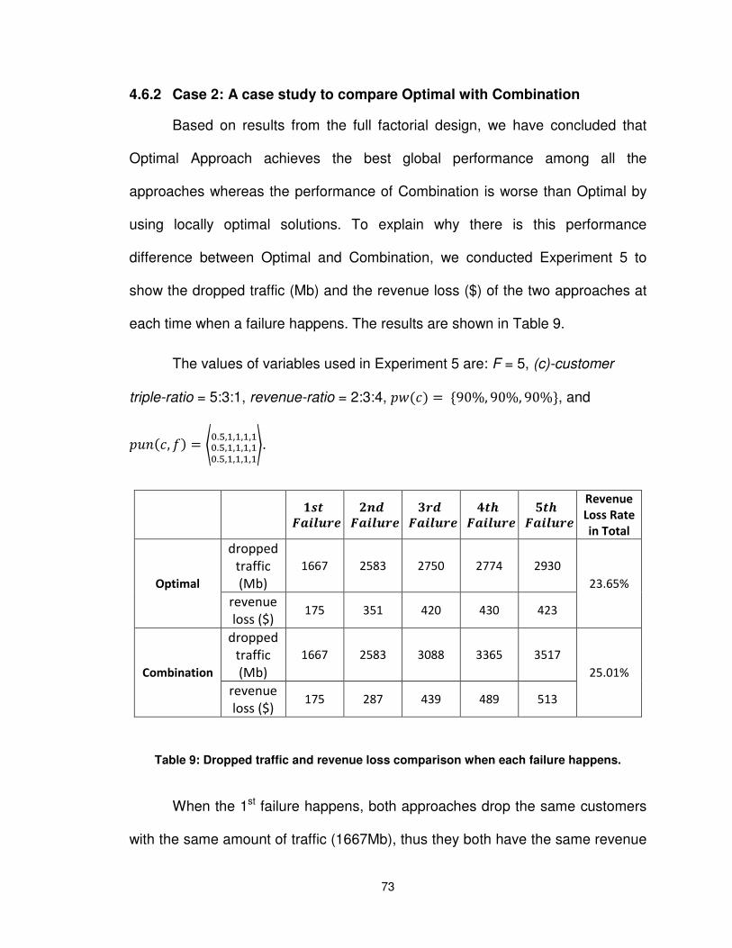
73

4.6.2 Case 2: A case study to compare Optimal with Combination

Based on results from the full factorial design, we have concluded that

Optimal Approach achieves the best global performance among all the

approaches whereas the performance of Combination is worse than Optimal by

using locally optimal solutions. To explain why there is this performance

difference between Optimal and Combination, we conducted Experiment 5 to

show the dropped traffic (Mb) and the revenue loss ($) of the two approaches at

each time when a failure happens. The results are shown in Table 9.

The values of variables used in Experiment 5 are: F = 5, (c)-customer

triple-ratio = 5:3:1, revenue-ratio = 2:3:4, �� ! B90%, 90%, 90%C, and

��, �� ! ��.�,�,�,�,��.�,�,�,�,��.�,�,�,�,��.

¦§¨ ¢¥©ª«¬

®¯° ¢¥©ª«¬

±¬° ¢¥©ª«¬

²¨³ ¢¥©ª«¬

´¨³ ¢¥©ª«¬

Revenue

Loss Rate

in Total

Optimal

dropped

traffic

(Mb)

1667 2583 2750 2774 2930

23.65%

revenue

loss ($) 175 351 420 430 423

Combination

dropped

traffic

(Mb)

1667 2583 3088 3365 3517

25.01%

revenue

loss ($) 175 287 439 489 513

Table 9: Dropped traffic and revenue loss comparison when each failure happens.

When the 1st failure happens, both approaches drop the same customers

with the same amount of traffic (1667Mb), thus they both have the same revenue

74

loss ($175). When the 2nd failure happens, both approaches drop the same

amount of traffic (2583Mb). Based on a locally optimal solution, the revenue loss

for Combination Approach is $287, whereas Optimal, based on a globally optimal

solution, drops different ��, �� customers and loses more revenue ($351).

Although Optimal Approach loses more revenue at the time when the 2nd failure

happens, it reduces the total amount of the traffic to be dropped for the 3rd, 4th,

and 5th failures by dropping different ��, �� customers. Therefore, the total

revenue loss rate for Optimal Approach (23.65%) is less than that for

Combination Approach (25.01%) at the end time ��.

4.6.3 Case 3: A case study on the predictor variable µ¶�·� Failure, Combination and Optimal approaches, as we found in the full

factorial design, achieve better performance by dropping customers who can

tolerate the first several interruptions or have not experienced any interruptions:

there is no revenue loss when choosing to drop the connections of these

customers. The value of �� is very informative in this regard: lower �� suggests that there are more customers who are not watching the VOD

programs and thus have experienced none or fewer interruptions; when �� is

low enough, there are enough such customers to enable an approach (such as

Failure, Combination and Optimal) to achieve zero revenue loss by dropping the

connections of these customers every time that a failure occurs. Therefore,

although only a minor effect of the predictor variable �� on the performance of

all approaches in the 2k factorial design was found, we closely examined the

contribution of �� to the zero revenue loss in Failure, Combination and

75

Optimal approaches in Experiment 5. The values of variables used in Experiment

5 are as follows: F = {1,2,3,4,5}; (c)-customer triple-ratio = 5:3:1; revenue-ratio =

2:3:4; pun�c, f� ! ��,�.�,�,�,��,�.�,�,�,��,�.0,�,�,��; pw�c� = {60%, 70%, 80%, 90%}. The revenue loss

rates for the three approaches are shown in Figure 4-10, Figure 4-11, and Figure

4-12.

Figure 4-10: Performance of Optimal Approach with varying µ¶�·�.

0

0.5

1

1.5

2

2.5

3

3.5

4

4.5

F= 1 F= 2 F= 3 F= 4 F= 5

Re

ve

nu

e lo

ss r

ate

(%

)


60%

70%

80%

90%

76

Figure 4-11: Performance of Failure Approach with varying µ¶�·�.

Figure 4-12: Performance of Combination Approach with varying µ¶�·�.

As expected, these three approaches show similar performance trends:

none of the performance trends in the figures are linear; all three approaches can

0

2

4

6

8

10

12

14

F= 1 F= 2 F= 3 F= 4 F= 5

Re

ve

nu

e lo

ss r

ate

(%

)


60%

70%

80%

90%

0

2

4

6

8

10

12

F= 1 F= 2 F= 3 F= 4 F= 5

Re

ve

nu

e lo

ss r

ate

(%

)


60%

70%

80%

90%

77

achieve zero revenue loss after the first several network failures, and there are

sudden increases in revenue loss rate with increasing number of failures. More

importantly, we can see the different influences of different values of �� from

high to low. When �� is 90%, all the approaches can keep the revenue loss to

zero for up to three failures. When �� is 80% and 70%, all the approaches

can keep the revenue loss to zero for up to four failures. When �� is 60%, all

the approaches can keep the revenue loss to zero for up to five failures. It is

interesting to note that when �� is 60%, the revenue loss rate can be kept at

zero for up to 5 failures even though ��, �� suggests that there will be

customers unsubscribing from the VOD service and thus revenue loss, if the

customers experience the second interruption.

4.6.4 Case 4: A case study for the time when failures happen

As mentioned in Section 3.2.2, we assume that there is a constant number

of new customers joining in the VOD service in each interval between two

adjacent failures, which implies that the failures are distributed evenly within the

real time period. Acknowledging that this assumption does not closely reflect

what happens in reality, its influence on the performance of all the approaches is

expected to be similar and thus does not affect our comparison of the

approaches in any significant way. To validate this expectation, we conducted

Experiment 6 and compared the performance of all six approaches in three

simulated situations with different failure distributions, assuming that all the new

customers are evenly distributed across real time intervals (each real time

interval could be a week, a month, etc.).

78

The three different failure distributions are:

In Simulation 1, F-1 failures occur at time �� and the last failure happens

at time ��. Therefore, before the F-1st failure no VOD connections are dropped

because no new customers join the network at time ��. The amount of traffic,

which is equal to X&��, caused by new customers joining the network between the

F-1st failure and the Fth failure is dropped at time �� when the last failure occurs;

In Simulation 2, the failures are evenly distributed in the operation period;

In Simulation 3, all failures occur at time ��.

It is important to note that in all three simulations, time �� refers to the

same time in real time to facilitate comparison: the amount of traffic caused by

new customers joining the network before time �� is the same in all three

different scenarios. So in Case 4, two extreme simulations are examined. In

Simulation 1, most new customers join the network after the F-1st failure but

before the Fth failure; in Simulation 3, most new customers join before the first

failure.

The values of variables used in Experiment 6 are: F = 5, (c)-customer

triple-ratio = 5:3:1, revenue-ratio = 2:3:4, �� ! B90%, 90%, 90%C, and ��, �� ! ��.�,�,�,�,��.�,�,�,�,��.�,�,�,�,��.

The results from the three simulations are shown in Figure 4-13.

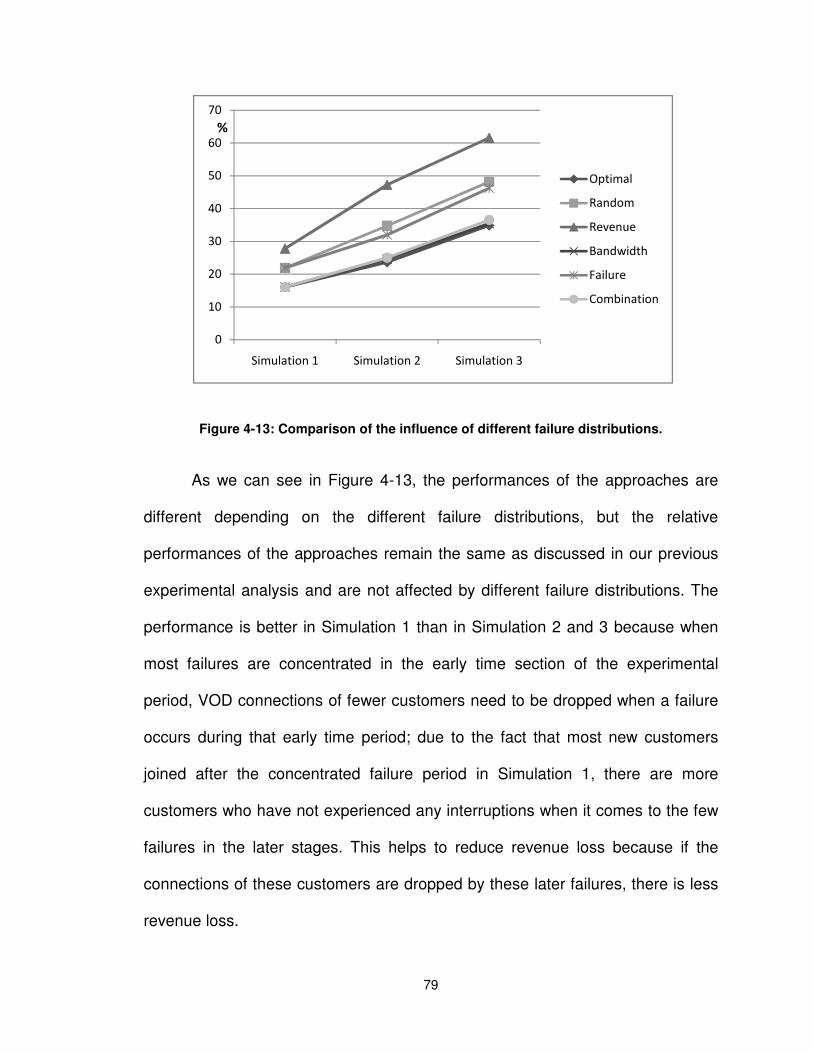
79

Figure 4-13: Comparison of the influence of different failure distributions.

As we can see in Figure 4-13, the performances of the approaches are

different depending on the different failure distributions, but the relative

performances of the approaches remain the same as discussed in our previous

experimental analysis and are not affected by different failure distributions. The

performance is better in Simulation 1 than in Simulation 2 and 3 because when

most failures are concentrated in the early time section of the experimental

period, VOD connections of fewer customers need to be dropped when a failure

occurs during that early time period; due to the fact that most new customers

joined after the concentrated failure period in Simulation 1, there are more

customers who have not experienced any interruptions when it comes to the few

failures in the later stages. This helps to reduce revenue loss because if the

connections of these customers are dropped by these later failures, there is less

revenue loss.

0

10

20

30

40

50

60

70

Simulation 1 Simulation 2 Simulation 3

Optimal

Random

Revenue

Bandwidth

Failure

Combination

%

80

4.7 Time Cost Analysis

The connections that have been selected to be saved must be reassigned

a wavelength in the surviving link within a very short period so that the customers

will not think they are interrupted. For example, a customer can tolerate a very

short interruption that lasts for less than 1 second and will not perceive it as an

“interruption”. Therefore, time cost must be examined and controlled quickly.

Time cost consists of two major parts, which can be controlled within an

acceptable range on the order of milliseconds.

a.) The time complexity of selecting ��, �� customers to be dropped

is �� & ��. To drop connections one by one, we must scan all ��, ��-customers (e.g. by looking at customer IDs), which leads to linear time

cost O(N) where N is total number of customers. Normally, the number

of customers may be up to tens of thousands in a 10Gb bandwidth

channel. Then based on the calculation speeds of currently popular

computers, the linear time cost is on the order of milliseconds.

b.) The time cost of reassigning the connections that have been selected

to be saved on a wavelength in the surviving link can be minimized in

20 milliseconds [44], which is considered acceptable.

81

5. CONCLUSIONS AND FUTURE WORK

In this project, we reviewed two major problems in cost-effective DWDM

networks: routing and wavelength assignment problem and traffic grooming

problem. Our objective is to minimize the cost either by minimizing the number of

wavelengths or SADMs to satisfy network connection requests, or by maximizing

the network throughput given certain wavelengths.

To minimize the revenue loss by selectively saving VOD connections

when a failure occurs in a DWDM network, we developed revenue focused semi-

protection approaches based on more realistic assumptions about DWDM ring

networks than those in [3]. Three statistics are used in our approaches: revenue

statistics, failure statistics, and bandwidth statistics. Our approaches can be

easily modified to adapt to real applications with real statistics. Our approaches

can also be applied to other network services that continuously occupy large

amounts of bandwidth, such as VOIP telephony, video conference service, and

web-based video services.

We used 2k and full factorial experimental designs to examine the impact

of predictor variables and the performance of our approaches. Results from

these studies suggest that even in a network with relatively low reliability, it is

possible to minimize the revenue loss or even reduce it to zero when failures

happen in the network without full protection. For example, in this study, we

found that a network could allow up to five failures during peak traffic time without

82

any revenue loss. By introducing bandwidth statistics, our approaches perform

better than those in [3]. Moreover, the new approach --- Bandwidth Approach ---

proposed in this project can achieve the best performance among all of the on-

line approaches.

In this project, we provide network operators with guidelines about how to

minimize the cost and improve the efficiency of their DWDM networks through a

review of current optimal solutions to RWA and traffic grooming problems. By

determining the relative importance of the five predictor variables and the

performance of the six semi-protection approaches, we also offer some insights

into how to minimizing revenue loss in their VOD service.

Future work can be done to explore semi-protection schemes for multicast

traffic patterns in DWDM networks. Multicast traffic models enable multiple

customers (or nodes) in a network to share common wavelengths with the same

or different VOD content. Moreover, as shown in [45], VOD connections of

customers who are ordering the same popular VOD program within a short time

window can be “batched” into one video stream to enable more customers to

share the same wavelength in a DWDM network. How to selectively save VOD

connections of customers in such a DWDM network with multicast traffic patterns

when failures happen is a complicated and challenging research question. We

expect that by properly rerouting and reassigning wavelengths, we can increase

the level of protection of the network while at the same time minimizing revenue

loss.

83

BIBLIOGRAPHY

[1] “14 Tbps over a Single Optical Fiber: Successful Demonstration of World's Largest Capacity,” Nippon Telegraph and Telephone Corporation, Sep. 2006. http://www.ntt.co.jp/news/news06e/0609/060929a.html.

[2] O. Gurel, C. Mas, I. Tomkos, “Requirements for a Transparent Pan- European Network,” Transparent Optical Networks, Proc., 6th International Conference, Vol. 1, pp.97-100, 2004.

[3] O. Gerstel, G. Sasaki, A. Balasubramanian, “Revenue Focused Protection for VOD in DWDM rings,” INFOCOM, 26th IEEE International Conference on Computer Communications, pp. 179-187, 2007.

[4] http://www.cisco.com, website of Cisco Systems Inc., Jan. 2007.

[5] http://www.huawei.com, website of Huawei Technologies Co. Ltd., 2008.

[6] G. Giambene, Queuing Theory and Telecommunications: Networks and Applications, Springer Science, New York, pg. 47, 2005.

[7] D. Barrett, T. King, Computer Networking Illuminated, Jones and Bartlett Publishers, ISBN 0-7637-2676-1, pg. 4, 2005.

[8] “Introducing DWDM”, Cisco Documentation, Cisco Systems Inc., 2000. http://www.cisco.com/univercd/cc/td/doc/product/mels/dwdm/dwdm_fns.htm#39797.

[9] O. Gerstel, P. Lin, G. Sasaki, "Combined WDM and SONET Network Design," in Proc. IEEE Infocom, pp. 734-743, 1999.

[10] M. Sridharan and A. K. Somani, “Revenue Maximization in Survivable WDM Networks,” in Proc. Optical Networking and Communications, SPIE, Vol. 1B, pp. 1012-1016, 1999.

[11] O. Gerstel and R. Ramaswami, “Optical Layer Survivability — a Service Perspective,” IEEE Communications Magazine, Vol. 38, pp. 104 – 113, Mar. 2000.

[12] Taehan Lee, Kyungsik Lee, and Sungsoo Park, “Optimal Routing and Wavelength Assignment in WDM Ring Networks,” IEEE Journal on Selected Areas in Communications, Vol. 18, No. 10, pp. 2146-2154, Oct. 2000.

[13] N.Wauters and P. Demeester, “Design of the Optical Path Layer in Multiwave-length Cross-connected Networks,” IEEE Journal on Selected Areas in Communications, Vol.14, pp. 881–892, 1996.

84

[14] R. Ramaswami, K. N. Sivarajan, Optical Networks: A Practical Perspective, 2nd Edition, San Mateo, CA, Morgan Kaufmann, pg. 455, 1998.

[15] B. Chen, G. N. Rouskas, R. Dutta, “Traffic Grooming in WDM Ring Networks to Minimize the Maximum Electronic Port Cost,” Optical Switching and Networking, Vol.2, Issue 1, pp. 1-18, May 2005.

[16] G. Wilfong, P. Winkler, “Ring Routing and Wavelength Translation,” in Proceedings of the 9th Annual ACM-SIAM Symposium on Discrete Algorithms, pp. 333–341, 1998.

[17] M. Garey, D. Johnson, G. Miller, and C. Papadimitriou, “The Complexity of Coloring Circular Arcs and Chords,” SIAM Journal on Algebraic Discrete Methods, pg. 216–227, 1980.

[18] R. Ramaswami and K. N. Sivarajan, “Routing and Wavelength Assignment in All-optical Networks,” IEEE/ACM Transactions on Networking, Vol. 3, pp. 489–500, Oct. 1995.

[19] C. Chen, S. Banerjee, “A New Model for Optimal Routing and Wavelength Assignment in Wavelength Division Multiplexed Optical Networks,” in Proc. IEEE Infocom ’96, pp. 164–171, Apr. 1996.

[20] K. C. Lee and V. O. K. Li, “A Wavelength Routing Algorithm in Wide-area All-Optical Networks,” Journal of Lightwave Technology, pp. 1218–1229, Vol. 14, June 1996.

[21] N.Wauters and P. Demeester, “Design of the Optical Layer in Multi-wavelength Cross-connected Networks,” IEEE Journal on Selected Areas in Communications, Vol.14, pp. 881–892, June 1996.

[22] T. Erlebach and K. Jansen, “The Maximum Edge-disjoint Paths Problem in Bidirected Trees,” SIAM Journal on Discrete Mathematics, Vol. 14, pp. 326–366, 2001.

[23] P. Saengudomlert, E. H. Modiano, R. G. Gallager, “Dynamic Wavelength Assignment for WDM All-Optical Tree Networks,” IEEE/ACM Transactions on Networking, Vol 13, No. 4, pp. 895-905, Aug. 2005.

[24] R. Datta, B. Mitra, S. Ghose, I. Sengupta, “An Algorithm for Optimal Assignment of a Wavelength in a Tree Topology and its Application in WDM Networks,” IEEE Journal on Selected Areas in Communications, Vol. 22, No. 9, pp. 1589-1600, Nov. 2004.

[25] A. Tucker, “Coloring a Family of Circular Arcs,” SIAM Journal on Applied Mathematics, Vol. 29, No. 3, pp. 493 – 502, 1975.

[26] I. A. Chlamtac, Ganz, and G. Karmi, “Lightpath Communications: An Approach to High Bandwidth Optical WAN’s,” IEEE/ACM Transactions on Networking, Vol. 40, pp. 1171–1182, 1992.

85

[27] D. K. Hunter and D. Marcenac, “Optimal Mesh Routing in Four-Fiber WDM Rings,” Electronics Letters, Vol. 34, No.8, pp. 796–797, 1998.

[28] Y. Xiong, Q. Zeng, Y. Cheng, Y. Zhou, “Wavelength Requirements in Wavelength-Routed Ring Networks,” Communications, Vol. 1, pp. 15-18, 1999.

[29] C. Nomikos, A. Pagourtzis, and S. Zachos, “Minimizing Request Blocking in All-optical Rings,” In Proc. of the 2003 IEEE INFOCOM, Vol. 2, pp. 1355-1361, Apr. 2003.

[30] P. J. Wan and L. Liu, “Maximal Throughput in Wavelength-Routed Optical Networks,” DIMACS Series in Discrete Mathematics and Theoretical Computer Science, Vol. 46, pp. 15–26, 1998.

[31] J.Q. Hu. “Optimal Traffic Grooming for Wavelength-division-multiplexing Rings with All-to-all Uniform Traffic,” OSA Journal of Optical Networks, Vol. 1, No. 1, pp. 32–42, 2002.

[32] O. Gerstel, G. Sasaki, and R. Ramaswami, “Cost Effective Traffic Grooming in WDM rings,” IEEE/ACM Transactions on Networking, Vol. 8, pp. 618-630, Oct. 2000.

[33] O.Gerstel, P. Lin, and G. Sasaki, “Wavelength Assignment in a WDM Ring to Minimize Cost of Embedded SONET Rings,” INFOCOM’98. Seventeenth Annual Joint Conference of the IEEE Computer and Communications Societies. Proceedings. IEEE Vol. 1, pp.94-101, 1998.

[34] L. Liu, X. Li, P. Wan, O. Frieder, “Wavelength Assignment in WDM Rings to Minimize SONET ADMs,” INFOCOM 2000, Vol. 2, pp. 1020-1025, 2000.

[35] R. Dutta and G. N. Rouskas, “On Optimal Traffic Grooming in WDM Rings,” Proceedings of the 2001 ACM SIGMETRICS, pp. 164-174, 2001.

[36] R. Dutta and G. N. Rouskas, “Traffic Grooming in WDM Networks: Past and Future,” IEEE Network, Vol. 16, pp. 46-56, Nov./Dev. 2002.

[37] J. Q. Hu, “Traffic Grooming in Wavelength-division-multiplexing Ring Networks: a Linear Programming Solution,” Journal of Optical Networking, Vol. 1, No. 11, pp. 397–408, Nov. 2002.

[38] N. Brauner, Y. Crama, G. Finke, P. Lemaire and C. Wynants, “Approximation Algorithms for the Design of SDH/SONET networks,” RAIRO Operations Research, pp. 235–247, 2003.

[39] O. Goldschmidt, D.S. Hochbaum, A. Levin and E.V. Olinick, “The SONET Edge-partition Problem,” Networks, Vol. 41, pp. 13–23, 2003.

[40] Y. Wang, Q.P. Gu, “Grooming of Symmetric Traffic in Unidirectional SONET/WDM Rings,” in Proceedings of IEEE ICC’06, pp. 2407-2414, 2006.

86

[41] Y. Wang, Q.P. Gu, “On the Complexity and Algorithm of Grooming Regular Traffic in WDM Optical Networks,” Journal of Parallel and Distributed Computing, Vol. 68, pp. 877-886, 2008.

[42] IXIA Leader in IP Performance Testing, “IPTV – Video Server Testing,” 2006. http://www.ixiacom.com/library/test_plans/display?skey=video_server.

[43] R. Jain, Art of computer Systems Performance Analysis Techniques For Experimental Design Measurements Simulation and Modeling, Wiley computer Publishing, John Wiley & Sons, Inc., 1991.

[44] X. Qin, and Y. Yang, “Multicast Connection Capacity of WDM Switching Networks With Limited Wavelength Conversion,” Networking, Vol. 12, Issue 3, pp. 526-538, June 2004.

[45] S. Kulkarni, “Bandwidth Efficient Video-on-demand Algorithm (BEVA),” in Proc. of International Conference on Telecommunications, Vol 2, pp. 1335-1342, 2003.

REVENUE FOCUSED SEMI-PROTECTION FOR VOD...

Documents

Transcript of REVENUE FOCUSED SEMI-PROTECTION FOR VOD...