RETROFITTING ANALYSIS TO INTEGRATE THE MIXALCO® …

RETROFITTING ANALYSIS TO INTEGRATE THE MIXALCO® PROCESS

TO THE CRUDE OIL DISTILLATION PROCESS

Thesis

By

LAURA PATRICIA PRADA VILLAMIZAR

Submitted to the Office of Graduate Studies of

Universidad de Los Andes

In partial fulfillment of the requirements for the degree of

M.SC. CHEMICAL ENGINEERING

August 2013

Major Subject: Chemical Engineering

Retrofitting analysis to integrate the MixAlco® process to the crude oil distillation

process

Copyright 2013 Laura Patricia Prada Villamizar

RETROFITTING ANALYSIS TO INTEGRATE THE MIXALCO® PROCESS

TO THE CRUDE OIL DISTILLATION PROCESS

Thesis

By

LAURA PATRICIA PRADA VILLAMIZAR

Submitted to the Office of Graduate Studies of

Universidad de Los Andes

In partial fulfillment of the requirements for the degree of

M.SC. CHEMICAL ENGINEERING

Approved by:

Chair of committee, Rocío Sierra Ramírez, PhD.

Committee Members, Jorge Mario Gómez, Phd.

Head of Department, Oscar Alvarez Solano, PhD.

August 2013

Major Subject: Chemical Engineering

i

ABSTRACT


process (August 2013)

Laura Patricia Prada Villamizar, Universidad de los Andes, Colombia

Advisor: Rocío Sierra Ramírez, Ph.D.

The MixAlco® technology comprises a processing facility to produce liquid

transportation fuels and/or value-added chemicals from biomass resources; however,

build and run a new MixAlco® plant may be very costly. On the other hand, high quality

and easily exploitable fossil-fuels resources inevitably dwindle worldwide. Both the

preservation of high quality fossil-fuel resources and the feasibility of a MixAlco® plant

can be importantly enhanced by retrofitting the MixAlco® process into an existing

fossil-fuel processing facility. This retrofitting is attainable because both processes have

similar products (bio-gasoline, gasoline, bio-jet, jet). This work assesses a retrofitting

analysis to integrate the MixAlco® process to a selected case of crude oil distillation

process (CODP). The proposed methodology suggests a hierarchy cost using the

following tools: process simulations, mass and energy integrations, and economic

evaluations. The work starts by assessing improvements for a base case of each of the

two involved plants separately. Then, comparisons between base cases and the

retrofitting of both processes (the resulting plant is regarded here as “integrated bio-

refinery”) is made. The most remarkable result was a Net Present Value (NPV)

ii

increment from MM USD 7.30 to MM USD15.7, and Return On Investment (ROI)

increment from 11.1% to 12.4% for MixAlco® process.

iii

RESUMEN


process (August 2013)

Laura Patricia Prada Villamizar, Universidad de los Andes, Colombia

Advisor: Rocío Sierra Ramírez, Ph.D.

MixAlco® es una tecnología donde se producen combustibles líquidos de

transporte y / o productos químicos de valor agregado a partir de fuentes de biomasa, sin

embargo, construir y operar una planta nueva de MixAlco® puede ser muy costoso. Por

otro lado, los recursos combustibles fósiles de alta calidad y fácilmente explotables

disminuyen en todo el mundo. La preservación de los combustibles fósiles de alta

calidad y la viabilidad de una planta MixAlco®, pueden mejorarse mediante la

integración del proceso MixAlco ® en una instalación existente de procesamiento de

combustibles fósiles.

Esta integración es posible gracias a que ambos procesos tienen productos

similares (bio-gasolina, gasolina, bio-jet, jet). Este trabajo evalúa un análisis de

integración entre el proceso de MixAlco® con el proceso de destilación de crudo de

petróleo (PDCP) como caso seleccionado. La metodología propuesta sugiere una

jerarquía de costos con las siguientes herramientas: simulación de procesos,

integraciones de masa y energía, y evaluaciones económicas. Este trabajo inicia

evaluando mejoras para un caso base en cada una de las plantas involucradas por

iv

separado. Después, se hacen comparaciones entre los casos base y la integración de los

dos procesos (la planta resultante se considera como "bio-refinería integrada"). El

resultado más importante para el proceso de MixAlco® presenta un incremento en el

Valor Presente Neto (VPN) de MM USD 7.30 a MM USD 15.7 y un incremento en la

tasa interna de retorno de la inversión (TIR) de 11.1% a 12.4%

v

ACKNOWLEDGEMENTS

I would like to thank my family for the love, belief, and support they have

provided me throughout my life, especially to my mother, Laura Villamizar. She gave

me much love and support, and thanks to my two brothers Dany and Sergio. I would like

to thank my two big loves Guillermo and Santiago, for their compression, support and

company all the time, especially during this work.

I would to express my deepest gratitude to Dr. Rocío Sierra, for her guidance,

and for her patience throughout this work. Thank you for all support during my graduate

study. I would like also to thank to all her group members for all their support and help.

I would like also to thank Cesar Mahecha for the support that he provide me

during this work.

vi

NOMENCLATURE

AEA: Aspen Energy Analyzer®

AFC: Annualized Fixed Cost

AGO: Atmospheric Gas Oil

APEA: Aspen Process Economic Analyzer®

API: Standard API gravity

BPD: Barrel Per Day

C: Cooler

CE: Chemical Engineering Plant Cost Index

CM: Compressor

CODP: Crude Oil Distillation Process

CON: Conveyor

CSTR: Continually Stirred Tank Reactors

DHFORM: Formation Enthalpy

DW&B: Direct Wage and Benefits

E: Heat Exchanger

EIA: US Energy Information Administration

FCI: Fixed Capital Investment

FOB: Free On Board

FOC: Fixed Operating Cost

vii

GAL: U.S liquid gallon, (231 in3)

GCC: Grand Composite Curve

H: Heater

HEN: Heat Exchange Network

HVGO: Heavy Vacuum Gas Oil

IRR: Internal Rate of Return

INHSPCD: In-house Pure Component Database

LVGO: Light Vacuum Gas Oil

M: Mixer

MACRS: Modified Accelerated Cost Recovery System

MOC: Minimum Operating Cost

MM: Million

MR: Cumulative Mass Lost

MS: Marshall and Swift Cost Index

MSA: Mass-Separating Agent

MTAC: Minimizing Total Annualized Cost

MW: Molecular weight

MW&B: Maintenance Wages and Benefits

Net_G: Net Generation

NF: Nelson-Farrer Refinery Construction Index

viii

NPV: Net Present Value

NREL: National Renewable Energy Laboratory

NRTL: Non-random-two-liquid

P: Pump

PBP: Payback Period

PSA: Pressure Swing Adsorption

R: Reactor

ROI: Return On Investment

RKS: Redlich-Kwong-Soave

S: Splitter

SCF: Standard Cubic Foot

SG: Standard specific gravity at 60°F

SP: Separator

T: Distillation tower

TBP: True Normal boiling point

TCI: Total Capital Investment

TEHL: Table of Exchangeable Heat Loads

TID: Temperature-Interval Diagram

TK: Tank

TR: Turbine

ix

TON: Metric ton (1,000kg)

USD: United States dollars

VFAs: Volatile Fatty Acids

VLSTD: Standard Liquid MolarVolume at 60°F

VOC: Variable Operating Cost

VP: Venture Profit

VS: Volatile Solids

WCI: Working Capital Investment

WWT: Waste Water Treatment

ZC: Critical Compressibility Factor

x

TABLE OF CONTENTS

Page

ABSTRACT .............................................................................................................. i

RESUMEN ................................................................................................................ iii

ACKNOWLEDGEMENTS ...................................................................................... v

NOMENCLATURE .................................................................................................. vi

TABLE OF CONTENTS .......................................................................................... x

LIST OF FIGURES ................................................................................................... xiii

LIST OF TABLES .................................................................................................... xv

1. INTRODUCTION ............................................................................................... 1

2. OBJECTIVES ..................................................................................................... 5

2.1 General objective ..................................................................................... 5

2.2 Specific objectives ................................................................................... 5

3. METHODOLOGY .............................................................................................. 6

3.1 Description of the proposed methodology .............................................. 6

3.1.1 Define needs ................................................................................. 6

3.1.2 Process arrangements .................................................................. 7

3.1.3 Feasibility .................................................................................... 7

3.2 Simulation Tools ........................................................................................... 9

3.2.1 MixAlco® process base case ........................................................ 9

3.2.2 CODP base case ............................................................................ 11

3.2.3 MixAlco® process and CODP retrofitted plant ............................ 14

xi

Page

3.3 Process integration ........................................................................................ 14

3.3.1 Material rerouting .......................................................................... 15

3.3.2 Heat Exchanger Network (HEN) .................................................. 16

3.3.3 Cost Analysis................................................................................. 16

4. RESULTS AND DISCUSSION ................................................................... 19

4.1 Simulation results .................................................................................... 19

4.1.1 Simulation builds up and results for MixAlco® base case ......... 19

4.1.1.1 MixAlco® block description .......................................... 21

4.1.1.2 MixAlco® overall mass balance results ......................... 54

4.1.1.3 MixAlco® overall heat balance results .......................... 56

4.1.2 Simulation builds up and results for CODP base case ................ 57

4.1.2.1 CODP Block description ................................................ 58

4.1.2.2 CODP overall mass balance results ............................... 68

4.1.2.3 CODP overall heat balance results ................................. 69

4.2 Define needs ............................................................................................ 69

4.3 Retrofitting procedure applied: Process arrangements ............................ 70

4.3.1 Internal rearrangements ............................................................... 70

4.3.1.1 MixAlco® process ......................................................... 70

4.3.1.2 CODP ............................................................................. 79

4.3.2 Internal modifications ................................................................. 84

4.3.2.1 MixAlco® process ......................................................... 84

xii

Page

4.3.2.2 CODP ............................................................................................ 95

4.3.3 External modifications ................................................................ 103

4.3.3.1 Case 1 ............................................................................. 105

4.3.3.2 Case 2 ............................................................................. 110

4.3.3.3 Comparison between cases ............................................. 123

4.4 Sensitivity analysis .................................................................................. 125

4.4.1 Variation of gasoline prices ......................................................... 125

4.4.2 Variation of Jet prices ................................................................. 126

4.4.3 Variation of Biomass prices ........................................................ 127

4.4.4 Variation of MixAlco® plant capacity ........................................ 127

CONCLUSIONS ....................................................................................................... 129

RECOMMENDATIONS AND FUTURE WORK ................................................... 132

REFERENCES .......................................................................................................... 134

APPENDIX A ........................................................................................................... 137

APPENDIX B ........................................................................................................... 153

APPENDIX C ........................................................................................................... 157

APPENDIX D ........................................................................................................... 159

APPENDIX E ............................................................................................................ 166

VITA ................................................................................................................ 177

xiii

LIST OF FIGURES

FIGURE Page

1-1 Pathways for converting biomass to hydrocarbon fuels .......................... 2

3-1 Flowchart of the proposed methodology ................................................. 8

3-2 Crude oil distillation TPB ....................................................................... 13

4-1 Blocks of MixAlco® process simulation. ............................................... 20

4-2 Feed handling simulation ........................................................................ 23

4-3 Pretreatment simulation ............................................................................ 25

4-4 Fermentation simulation .......................................................................... 29

4-5 Dewatering simulation ............................................................................ 34

4-6 Ketonization simulation .......................................................................... 39

4-7 Lime kiln simulation ............................................................................... 43

4-8 Final simulation ....................................................................................... 46

4-9 Distillation curve for gasoline ................................................................. 49

4-10 Distillation curve for Jet ............................................................................. 50

4-11 Gasification simulation... ........................................................................... 51

4-12 Blocks of CODP simulation ....................................................................... 57

4-13 First pre-heating train ................................................................................. 58

4-14 Second pre-heating train ............................................................................. 61

4-15 Atmospheric distillation column ............................................................... 63

4-16 Vacuum distillation column ....................................................................... 66

4-17 Mass integration for MixAlco® process .................................................... 73

xiv

FIGURE Page

4-18 Power integration for MixAlco® process .................................................. 73

4-19 Heat integration in Reactors for MixAlco® process .................................. 74

4-20 Cash flow for MixAlco® process in the base case .................................... 79

4-21 Hot and Cold composite for MixAlco® HEN............................................ 87

4-22 Grand composite curve for MixAlco® HEN ............................................. 87

4-23 Grid diagram for MixAlco® HEN ............................................................. 89

4-24 Cash flow for MixAlco® process with HEN ............................................. 95

4-25 Hot and Cold composite for CODP HEN .................................................. 97

4-26 Grand composite curve for CODP HEN .................................................... 97

4-27 Grid diagram for CODP HEN .................................................................... 99

4-28 MixAlco® and CODP simulation integrated ............................................. 104

4-29 Cash flow of MixAlco® process in case 1 ................................................. 109

4-30 Hot and Cold composite for case 2 ............................................................ 112

4-31 Grand composite curve for case 2 .............................................................. 113

4-32 Grid diagram for case 2 .............................................................................. 115

4-33 Cash flow of MixAlco® process in case 2 ................................................. 123

4-34 Variation of gasoline price for MixAlco® process .................................... 125

4-35 Variation of Jet price for MixAlco® process ............................................. 126

4-36 Variation of Biomass price ......................................................................... 127

4-37 Variation of MixAlco® plant capacity ....................................................... 128

xv

LIST OF TABLES

TABLE Page

3-1 Biomass feed composition for MixAlco® process .................................... 10

3-2 MixAlco® operating conditions ................................................................. 11

3-3 Assay data for crude oil .............................................................................. 12

3-4 Assay data for crude oil Light ends ............................................................ 12

3-5 CODP operating conditions ....................................................................... 13

3-6 Feedstock, utilities and product prices ....................................................... 17

4-1 Feed handling mass and heat balance ........................................................ 24

4-2 Heat balances for Feed Handling equipment ............................................. 24

4-3 Pretreatment mass and heat balance ........................................................... 27

4-4 Fermentation mass and heat balance .......................................................... 30

4-5 Heat balances for Pretreatment and Fermentation equipments .................. 33

4-6 Dewatering mass and heat balance ............................................................. 35

4-7 Heat balances for Dewatering equipments ................................................. 38

4-8 Ketonization mass and heat balance ........................................................... 40

4-9 Heat balances for Ketonization equipments ............................................... 42

4-10 Heat balances for Lime kiln equipments .................................................... 43

4-11 Lime kiln mass and heat balance ................................................................ 44

4-12 Final mass and heat balance ....................................................................... 46

4-13 Heat balances for Final equipments ........................................................... 49

xvi

TABLE Page

4-14 Gasification mass and heat balance ............................................................ 52

4-15 Heat balances for Gasification equipments ................................................ 53

4-16 MixAlco® yields ........................................................................................ 54

4-17 Summary fo heat balances for MixAlco® processs ................................... 56

4-18 First train preheating mass and heat balance .............................................. 59

4-19 Heat balances for equipments in 1st preheating train ................................ 60

4-20 Second train preheating mass and heat balance ......................................... 62

4-21 Heat balances for equipments in 2nd preheating train ............................... 62

4-22 Atmospheric distillation mass and heat balance ........................................ 64

4-23 Heat balances for equipments in atmospheric distillation unit .................. 65

4-24 Vacuum distillation mass and heat balance ................................................ 67

4-25 Heat balances for equipments in vacuum distillation unit ......................... 68

4-26 CODP Yields .............................................................................................. 68

4-27 Overall heat balances for CODP ................................................................ 69

4-28 Fresh MixAlco® streams ........................................................................... 71

4-29 Waste MixAlco® streams .......................................................................... 72

4-30 VOC of MixAlco® process in base case.................................................... 75

4-31 FOC of MixAlco® process in base case .................................................... 76

4-32 FIC of MixAlco® process in base case ...................................................... 77

4-33 Summary MixAlco® economic results in base case .................................. 77

4-34 Fresh CODP streams .................................................................................. 80

xvii

TABLE Page

4-35 Waste CODP Streams ................................................................................ 81

4-36 FCI for CODP in base case ........................................................................ 82

4-37 VOC for CODP in base case ...................................................................... 82

4-38 FOC for CODP in base case ....................................................................... 83

4-39 MixAlco® process streams for HEN ......................................................... 85

4-40 Heat integration for MixAlco® process ..................................................... 88

4-41 Heat exchangers for MixAlco® HEN ........................................................ 90

4-42 Coolers for MixAlco® HEN ...................................................................... 90

4-43 Heaters for MixAlco® HEN ...................................................................... 91

4-44 VOC of MixAlco® process with HEN ...................................................... 92

4-45 FOC of MixAlco® process with HEN ....................................................... 93

4-46 Summary MixAlco® economic results with HEN..................................... 94

4-47 Process streams for CODP ......................................................................... 96

4-48 Summary of HEN cases for CODP ............................................................ 98

4-49 Heat exchangers in the best CODP case .................................................... 100

4-50 Coolers in the best CODP case .................................................................. 101

4-51 Heaters in the best CODP case ................................................................... 102

4-52 VOC of CODP with HEN .......................................................................... 102

4-53 Heat integration for MixAlco® and CODP in case 1 ................................ 106

4-54 VOC of MixAlco® process in case 1 ......................................................... 106

4-55 FOC of MixAlco® process in case 1 ......................................................... 107

xviii

TABLE Page

4-56 Summary MixAlco® economic results in case 1 ....................................... 108

4-57 Process streams for case 2 .......................................................................... 110

4-58 Heat integration for MixAlco® and CODP case 2..................................... 114

4-59 Heat exchangers for case 2 ......................................................................... 115

4-60 Coolers for case 2 ....................................................................................... 118

4-61 Heaters for case 2 ....................................................................................... 119

4-62 VOC of MixAlco® process in case 2 ......................................................... 120

4-63 VOC of CODP in case 2 ............................................................................ 120

4-64 FOC of MixAlco® and CODP in case 2 .................................................... 121

4-65 Summary MixAlco® and CODP economic results in case 2 .................... 122

4-66 Heat integration comparison of cases ......................................................... 124

4-67 Economic comparison of cases .................................................................. 124

1

1. INTRODUCTION

World liquid fuels consumption grew by 0.800 MM bpd in 2012. US Energy

Information Administration (EIA) expects consumption growth will be higher over the

next two years, at 0.900 million bpd in 2013 and 1.20 MM bpd in 2014 (EIA, 2013).

However, the liquid fuel production is estimated to be decline. Furthermore, the price of

crude oil is very sensitive to international politic issues. Clearly, new alternatives for

renewable fuels are necessary.

The MixAlco® technology, invented by Professor M. Holtzapple at Texas A&M

University (Holtzapple, 2009), comprises a processing facility to produce liquid

transportation fuels and/or value-added chemicals from sustainable resources.

MixAlco® converts materials such as municipal solid waste (MSW), sewage sludge,

forest product residues, and non-edible energy crops such as sweet sorghum into a wide

array of chemicals and secondary alcohols that can be further refined through separate,

well-established processes to produce renewable gasoline, jet fuel or diesel. The bio-

gasoline produced through the MixAlco® technology is not ethanol. In fact, it has a

higher energy value than ethanol and can be blended directly with gasoline produced

from hydrocarbons. (Terrabon, 2010).

MixAlco® process comprises a fermentation stage, which employs a mixed culture

of acid-forming microorganisms that convert biomass components (carbohydrates,

proteins, and fats) to carboxylate salts. Depending on the choice of buffer, the salts may

2

be ammonium carboxylates (buffered by NH4HCO3) or calcium carboxylates (buffered

by CaCO3) among others. Via pathway C in Figure 1-1, calcium carboxylates are

thermally converted into ketones, which are subsequently hydrogenated into a mixture of

secondary alcohols. Finally, these alcohols are chemically converted into hydrocarbon

fuels (gasoline, jet fuel, and diesel) (Pham, Holtzapple, & El-Halwagi, 2010). In

Appendix A, details on the MixAlco® process are briefly discussed.

Figure 1-1. Pathways for converting biomass to hydrocarbon fuels (Pham et al., 2010)

Build and run a new plant, such as the one required for the MixAlco® process, is

very costly; however, its economic performance may be greatly enhanced by retrofitting

analysis. This strategy comprises adding a bio-fuels plant like MixAlco® process to an

existing fossil fuel plant like a crude oil distillation process (CODP).

3

This mechanism is beneficial for both parties because an inexpensive increase of

the production capacity of the refinery may be obtained, while economic matters for the

biofuels-producing plant are resolved. The systems obtained by integrating a biomass

fuel plant to the fossil fuel plant is regarded here as bio-refineries or integrated fossil

bio-refineries.

Basically, CODP comprises a preheating train where crude oil is fed from the

holding tank; then vaporized in the furnace where the combustion of a fuel is taking

place. Finally, it is fed to the bottom of the distillation column. The distillation column is

considered the master unit since all different cuts like light and heavy naphtha, kerosene,

light and heavy gas oils, and atmospheric residue are separated and purified. The

vacuum distillation unit further distills residual bottoms from the atmospheric tower,

where different cuts can be obtained like atmospheric, light vacuum, and heavy vacuum

gas oil. A large amount of heat is transported out to the preheating train from the

condenser, the end products, the strippers and the pumparounds.

The substantial energy requirement of crude oil distillation columns is met partly

by costly utilities, such as steam and fuel for fired heaters, and partly by heat recovered

from the process, using process-to-process heat exchange. Energy savings, therefore,

demand not only a distillation column that is energy-efficient, but also a heat exchanger

network (HEN) which minimizes utility costs by maximizing heat recovery. (Benali &

Tondeur, 2011). The CODP in this work corresponds to a modified version of a

4

distillation unit of Ecopetrol. Modifications were necessary to protect intellectual

property rights.

This work assesses a retrofitting analysis to integrate the MixAlco® process to

the crude oil distillation process. Focus is given to the problem of process modification

to the crude oil distillation system by considering increase the process profitability and

material substitution with biomass feedstocks. The approach proposed for this analysis

was developed by B. Cormier under the advisory of Dr. M. El-Halwagi at Texas A&M

University (Cormier, 2005). The proposed hierarchy is based on costs analysis and

involves internal process modification, operating-condition adjustment, and feedstock

substitution. If is needed, new units are added followed by the incorporation of new

production lines. Then, heat and mass integration techniques are used to link the units

and streams. (Cormier, 2005)

The competitiveness of markets nowadays and the focus on energy efficiency

requires improved heat-integrated process designs. Aspen Energy Analyzer® (AEA)

working in concert with flowsheet simulators such as Aspen Plus® provides an easy

environment to perform optimal heat exchanger network design and pinch analysis.

For the economic evaluation, an Aspen Process Economic Analyzer® (APEA)

provides benefits that will be explored in this study.

http://www.aspentech.com/products/aspen-plus.aspx

5

2. OBJECTIVES

2.1 General Objective

Apply a retrofitting analysis to integrate into a crude oil distillation system, the

MixAlco® process using the kenitonization route.

2.2 Specific Objectives

Conduct process integration studies to determine cost-effective strategies for

enhancing production incorporating the MixAlco® process into the crude oil

distillation system.

Develop several energy and mass integration approaches and use them to induce

synergism and to reduce cost by exchanging heat, material utilities, and by

sharing equipment.

Develop cost-benefit analysis to guide the decision-making process and to

compare various production routes.

6

3. METHODOLOGY

Results from a previous work on MixAlco® process economics were used as a base

case (Pham et al., 2012). In that work, the economics of the calcium carboxylate

platform (pathway C in Figure 3-1) using municipal solid waste or sugarcane bagasse as

feedstock were estimated. On this basis, the following MixAlco® process features were

used: no requirement for sterility or any external enzymes, low capital cost, and cost-

effective dewatering, which comprise the use of an effective evaporation system, briefly

explained in Appendix A. In the previous work, the minimum selling prices of

hydrocarbon fuels reported can be around 1.57 USD /gal if municipal solid waste is

available at the US average tipping fee of 45 USD/dry ton (40 ton/h plant, with internal

hydrogen production). (Pham et al., 2012)

Retrofitting analysis was performed using the methodology developed by Cormier &

El-Halwagi developed on the framework of mass and energy process integration. An

overview of the methodology is shown in Figure 3-1 (Cormier, 2005). An explanation is

found in Section 3.1.

3.1 Description of the proposed methodology

3.1.1 Define needs

In the first step for the retrofitting analysis, it is possible to define the

opportunities in the processes that would result in an increased profitability.

7

3.1.2 Process arrangements

Figure 3-1 shows three building blocks that are arranged in order of increasing cost.

The definition of each block is explained below (Cormier, 2005):

- Internal rearrangements: The goal is to reach the production target using low cost

strategies. These include process reconfiguration (e.g., stream rerouting) and

modification of operating conditions.

- Internal modification by adding new units: it is aimed to pursue medium-cost

modifications. These include required addition of new units, and/or replacement of

the existing units with new ones.

- External modification by adding new lines: Capital-intensive strategies are

invoked. These include the addition of new production lines.

3.1.3 Feasibility

Once two candidates are integrated into the current plant by heat and mass

integration, the ROI can be calculated. The decision to go deeper into the analysis

depends on the obtained value. (Cormier, 2005)

8

Figure 3-1. Flowchart of the proposed methodology (Cormier, 2005).

Define needs

Internal

rearrangements

only

Simulation

improvement

Cost analysis

Feasible?

Internal

modification by

adding new units

Simulation

improvement

Cost analysis

Feasible?

External

modification by

adding separated

lines

Simulation

improvement

Cost analysis

Proposal to the

company

Feasible?

Medium Cost

Low Cost

High Cost

Redefine needs

Internal rearrangements:

Process Reconfiguration

Modification of Operating Conditions

Internal Modifications:

Add New units


External Modifications:

Add new lines


Yes

Yes

Yes

9

3.2 Simulation Tools

Regardless to existence of specialized software for petroleum industry (Aspen

Hysys® and PRO II®), Aspen Plus® software was used according a specific database

that estimates most of the desired properties of biomass.

Initially, each one of these two base cases was simulated separately. Then, both

plants were put together in a single worksheet to make integrations possible.

Specificities of each of these simulation cases are given below. For all simulations, the

following three steps were necessary:

- Flow sheet definition: All inlet and outlet streams to the different stages in both

the MixAlco® and the CODP systems, as well as all unit operations and their

interconnecting streams were defined.

- Chemical components: All chemical components in the system, from reagents

to intermediates and products were specified during simulations. Appendix B

shows the properties for each of the substances used in the simulations..

- Operating conditions: The operating conditions, such as temperature, pressure,

heat duties etc., for each unit operation were specified for each process in next

sections.

3.2.1 MixAlco® process base case.

The simulation was made using the National Renewable Energy Laboratory

(NREL) database In-house Pure Component Database (INHSPCD). Within this tool,

10

estimation of most of the properties of biomass components such as glucose, xylose,

cellulose, xylan, lignin were possible. Components other than the ones listed above, are

identified within this database as solslds. (Wooley & Putsche, 1996).

As Wooley and Putsche, (1996) suggested, the thermodynamic package used in

this simulation was non-random-two-liquid (NTRL), where NRTL liquid include

activity coefficient model, Henry’s law for the dissolved gases, and Redlich-Kwong-

Soave (RKS) equation of state for the vapor phase.

The MixAlco® process simulation was made for a capacity of 40.0 ton/h of

biomass. The biomass feedstock in the simulation was a mixture 80.0% - 20.0% w/w of

sugarcane bagasse (like carbohydrate source) and chicken manure (like secondary

nutrient source) respectively. Table 3-1 shows the biomass feed composition. Other

details on the feedstock stream (e.g., properties) are shown with simulation results in

Section 4.1.1.1.

Table 3-1. Biomass feed composition for MixAlco® process

Component Feedstock

ton/h %w/w

Cellulose 16.8 43.0

Hemicellulose (xylan) 7.50 19.0

Lignin 10.0 25.0

Solslds 5.20 13.0

Total 40.0 100

Operating conditions used for simulation of all MixAlco® unit operations are

shown in Table 3-2.

11

Table 3-2. MixAlco® operating conditions

Process Parameter Value

Feed handling Temperature (°C) 55.0

Pressure (bar_a) 1.00

Pretreatment Temperature (°C) 55.0


Fermentation Temperature (°C) 55.0


Ketonization Temperature (°C) 430


Ketone hydrogenation Temperature (°C) 130


Lime kiln Temperature (°C) 500


Alcohol dehydration Temperature (°C) 300


Oligomerization Temperature (°C) 300


Olefin hydrogenation Temperature (°C) 130


Gasification Temperature (°C) 760


Steam-gas shift Temperature (°C) 254


3.2.2 CODP base case.

The CODP simulation was made using Grayson Streed and Braun k-10 (BK10)

as thermodynamic packages, for a crude oil load of 27,012 bpd (162 ton/h) and 22.8

API. Because, Grayson property methods were developed for systems containing

hydrocarbons and light gases and BK10 property method is suited for vacuum and low

pressure applications. (Aspen plus®, 2013). Table 3-3 and 3-4 shows the assay data.

The crude oil distillation curve is presented in Figure 3-2.

12

Table 3-3. Assay data for crude oil****

%Distilled* Molecular Weight Specific

Gravity

Sulfur

curve**

Viscosity***

(80ºC)

Viscosity***

(100ºC)

0.929 71.0 0.646

2.54 97.0 0.725

5.46 116 0.759 5x10-3

8.71 144 0.788 0.0190

11.5 153 0.810 0.0500

13.7 171 0.823 0.0790

16.6 186 0.838

21.9 206 0.862 0.322

28.8 250 0.872

36.6 280 0.897 0.808

41.3 323 0.920 9.13 5.80

44.9 357 0.921 0.995 10.3 5.79

53.8 378 0.932 18.0 10.3

62.1 436 0.946 1.19 43.3 22.5

67.3 514 0.956 1.42 77.8 34.5

85.0 1,247 1.03 289,150 31,971

Molecular weight:

288

Bulk value:

0.0488

*Mid-percent distilled (same basis as distillation data, i.e., volume or weight)

**Given in %w/w

***Given in centistokes

****Data supply by Ecopetrol

Table 3-4. Assay data for crude oil Light ends**

Component* % Mass

C2 0.212

C3 3.60

IC4 5.40

NC4 14.5

IC5 24.4

NC5 23.5

Hexane 28.4

Total % light ends in the assay 0.940

*The number after C refers to the number of carbons in the alkane molecule. I is for iso (non-linear)

structures and N for straight chains

**Data supply by Ecopetrol

13

Figure 3-2. Crude oil distillation TPB

Operating conditions used for the atmospheric and vacuum columns are shown in

Table 3-5.

Table 3-5. CODP operating conditions


Column T-204 - Atmospheric tower

Heat duty condenser (kJ/s) 7,206

Tray crude feed 17.0

Tray steam feed 19.0

Tray number 19.0

Condenser Partial

Temperature tray 1 (°C) 98.0

Temperature tray 19 (°C) 366

Pressure tray 1 (bar_a) 1.70


Heat duty pumparound MPA (kJ/s) 5,113

Heat duty pumparound MPACAL (kJ/s) 563

Column T-205- Vaccum tower

Heat duty condenser (kJ/s) 308

Tray crude feed 7.00

Tray steam feed 8.00

Tray number 8.00

14


Condenser Partial

Temperature tray 1 (°C) 60.0

Temperature tray 8 (°C) 389



Heat duty pumparound UPA (kJ/s) 2,117

Heat duty pumparound MPA (kJ/s) 5,874

Heat duty pumparound MPACAL (kJ/s) 219

3.2.3 MixAlco® process and CODP retrofitted plant

The simulation of MixAlco® process and CODP integrated was made from the base

case of each plant, so the operating conditions and feedstock properties were the same

shown in sections 3.2.1 and 3.2.2; regarding the thermodynamic package: NTRL and

Grayson Streed.

3.3 Process integration

The design of any industrial process relies on process simulators and programs for

unit operation design. The core of process design rests on two important dimensions:

mass and energy. Mass involves the creation and routing of chemical species in reaction,

separation, and byproduct/waste-processing systems. These constitute the heart of the

process and define a company´s technology base. Energy provides the necessary heating,

cooling, and shaftwork for those systems.

Because most industrial processes are complicated, performance and economics

depend not only on proper selection and design of individual components but also on

15

proper assembling of building blocks. Fundamental principles can guide this assembly.

Process integration comprises all means to achieve the goals of optimal assembly and

performance. In process integration, the unity of the entire process is emphasized.

Pinch analysis is the most successful way to achieve energy integration; which impacts

mainly in process economics. Mass integration, on the other hand, has received great

attention and development, because it directly impacts process performance. (El-

Halwagi & Spriggs, 1998).

For this, material rerouting and heat exchanger network (HEN) were considered

(Cormier, 2005).

3.3.1. Material rerouting

Mass integration is a systematic methodology that provides a fundamental

understanding of the global flow of mass within the process and employs this

understanding. To apply this integration the following steps were used:

Analysis: Detect the minimum fresh resource consumption and minimum waste

discharge streams.

Retrofit: Modify an existing water-using network to maximize water reuse and

minimize wastewater generation through effective process changes (Cormier,

2005).

For additional details about this type of integration see Appendix C.

16

3.3.2 Heat Exchanger Network (HEN)

In the plant, heating and cooling represent an important operating cost. In order to

minimize the operating cost for the heat utilities, heat integration is needed. The

following multiple design objectives are pursued:

Minimize the investment cost of the units (i.e., surface area of exchanger, heater

and/or cooler).

Minimize the operating cost of utilities (steam, cooling water, etc).

Minimize the number of units (i.e., heat exchanger). (Cormier, 2005)

In this work, energy integration was performed using Aspen Energy Analyzer®

(AEA) in compliance to all license agreements. For additional details about this type of

integration see Appendix D.

3.3.3 Cost Analysis

Many technical and environmental decisions during process design are strongly

impacted by economic factors; therefore, an essential component of any sustainable

design is an economic analysis, which is performed on the basis of total investment and

operating costs. (El-Halwagi, 2012). Typically, a minimum of 15.0% for the ROI is

pursued. If this is not achievable, ROIs of 5.00 to 10.0% may be acceptable under

17

current market conditions. (Cormier, 2005) Additional details about economic analysis

concepts are presented in Appendix E.

In this work, the prices for feedstocks, chemicals and material disposal for

MixAlco® process were taken from Pham et al., (2012). The prices of crude oil were

taken from the EIA official website. The utilities costs were taken from the database of

AEA except for the steam cost, which was taken from Seider, (2004). Finally, the prices

for refinery products were found in the EIA official website. Appendix D shows the

price profile for these products. For Atmospheric Gas Oil (AGO) and Light Vacuum Gas

Oil (LVGO) prices, a factor of 10% from the price of Heavy Vacuum Gas Oil (HVGO)

was used. All these prices are shown in Table 3-6.

Table 3-6. Feedstock, utilities and product prices

Item Costs and Prices

(USD / unit)

Fee

dst

ock

cost

s

Sugarcane bagasse (USD/ton) 60.0

Chicken manure (USD/ton) 10.0

Crude oil (USD/ton) 643

Crude oil (USD/barrel) 93.4

Quick Lime (USD/ton) 70.0

Flocculant (USD/ton) 991

Iodoform (USD/kg) 25.0

CaCO3 (USD/ton) 50.0

Material disposal (USD/ton) 18.0

Uti

liti

es c

ost

Fired Heat (USD/ton) 2.55

MP Steam (USD/ton) 4.36

Cooling Water (USD/m3) 4x10-3

LP Steam (USD/ton) 4.17

Refrigerant (USD/m3) 0.0130

Electricity (USD/kWh) 0.0620

Steam @ 353°C (USD/ton) 10.0

Steam @ 454°C (USD/ton) 10.0

18

Item Costs and Prices

(USD / unit) P

rod

uct

s se

llin

g

pri

ces

Gasoline (USD/gal) 3.28

Jet (USD/gal) 2.88

Diesel (USD/gal) 3.75

AGO (USD/gal) 2.40

LVGO (USD/gal) 2.30

HVGO (USD/gal) 2.20

Asphalt (USD/gal) 1.30

19

4 RESULTS AND DISCUSSION

Simulation results are presented for each one of the two base cases (MixAlco® and

COPD). This simulations were necessary in order to be able to compare MixAlco®

alone vs MixAlco® retrofitted within a COPD plant. Then, the methodology for

retrofitting (shown in Figure 3-1) will be followed, which eventually (third loop)

conduces to the results obtained for the combined MixAlco®-COPD integrated plant.

An economic analysis is presented for each one of the integration possibilities and for

the combined MixAlco®-COPD. Extensive comparisons are presented at the end. The

Enthalpy reported by Aspen Plus® is in their standard states at 1 atm and 298.15°K.

4.1 Simulation results

In this section, simulation building procedures as well as relevant results of each one

of the base cases are discussed next (MixAlco® base case and COPD base case).

4.1.1 Simulation builds up and results for MixAlco® base case

The MixAlco® simulation was divided in seven blocks to build up a simulation,

as shown in Figure 4-1.

These blocks are listed and explained below:

1. FEED-HAN: Feed handling process

2. PRET -FER: Pretreatment and fermentation process

3. DEWATER: Dewatering process.

4. KETONIZA: Ketonization and ketone hydrogenation processes.

20

5. LIME-KIL: Lime kiln process.

6. FINAL: Dehydratation, oligomerization and saturation processes.

7. GASIFICA: Gasification reactor, steam gas shift reactor, and adsorption process

Figure 4-1. Blocks of MixAlco® process simulation

21

4.1.1.1 MixAlco® Block description

- Feed Handling (Unit 1)

The Feed Handling block exists only for simulation purposes and it is meant: (i) to mix

the reacting substances (biomass, water, and lime) to prepare them for pretreatment and (ii)

to obtain lime (Ca(OH)2) from quick lime (CaO) as shown in Equation 4-1.

(4-1)

Quick lime Lime

In the actual MixAlco® process, feed handling would occur simultaneously (in the

same unit) with pretreatment. This is because the reaction in Eq. 4-1 is exothermic

(Enthalpy of reaction obtained was 1.960kJ/s shown in Table 4-2); thus, it is advantageous

to use the reaction heat to obtain an increase of temperature necessary for pretreatment to

occur at a measurable rate. Because in the simulation feed handling and pretreatment were

not put in the same unit, this fact could not be considered. Instead, an external source of

heat was implemented for the pretreatment stage.

Two sources for quick lime were considered: The first is CaO produced in-site and

the second is make-up fresh quick lime. The quick lime that is produced in site comes from

the LIME-KIL block explained in a later section. The stream that carries this reactant has

been labeled as CAO-RECY in Figure 4-2. As shown in Table 4-1, this stream contains

4.06 ton/h of CO2 which corresponds to 44.0% w/w of the stream composition. This gas is

22

a reaction byproduct which in the actual process is expelled as it is produced, but in this

simulation has to be carried all the way to the end gasification block in the SP-115. The

unit operation CON-101 is a conveyor set up to transport this recycled stream. On the other

hand, the fresh, make-up CaO (labeled as CAO-MAKE in Figure 4-2) is purchased with a

cost of 70.0USD/ton. The mass ratio CAO:CAO-MAKE is 1:10 which clearly shows that a

lime recovery process is represented in a saving operating cost. In addition a water fed at a

flow rate of 2ton/h, stream labeled as H2O-LIME in Figure 4-2 was considered.

For the reaction (Eq. 4-1, occurring in R-101), a conversion factor of 1 was

employed, although the reactants (i.e., water and quick lime) were fed in exact

stoichiometric amounts (i.e., no reactant was fed in excess). (Gosseaume, 2011).

Two streams leave this block: (i) Stream 1(OUT) in Figure 4-2 required for the

reactor convergence and after a mixing unit (TK-101) (ii) Stream (BIOM-LIM(OUT))

which is the stream that contains biomass mixed with water and lime and goes to

pretreatment.

Results from mass and heat balance in the simulation for this block are shown per

stream in Table 4-1. On the other hand, the heat balance for the equipment in this block is

shown in Table 4-2, where the conveyor power consumption is very low.

23

Figure 4-2. Feed handling simulation

24

Table 4-1. Feed handling mass and heat balance

BIOMASS CA-BIO CA-BIOM CAO CAO-MAKE CAO-RECY H20-LIME

Temperature (°C) 25.0 55.0 55.0 55.0 55.0 55.0 25.0

Pressure (bar_a) 1.00 1.00 1.00 1.00 1.00 1.00 1.00

Mass vapor fraction 0 0.0800 0.0800 0.440 0 0.440 0

Mass solid fraction 0.870 0.820 0.820 0.560 1.00 0.560 0

Mass flow (ton/h) 39.5 51.6 51.6 9.24 0.900 9.24 2.00

Enthalpy (kJ/s) 80,720 120,205 120,205 26,310 2,824 26,310 8,809

Component mass flow (ton/h)

CELLU-01 16.8 16.8 16.8 0 0 0 0

XYLAN 7.50 7.50 7.50 0 0 0 0

LIGNI-01 10.0 10.0 10.0 0 0 0 0

SOLSL-01 5.17 5.17 5.17 0 0 0 0

SOLUN-01 0 0 0 0 0 0 0

WATER 0 0.0500 0.0500 0 0 0 2.00

CO2 0 4.06 4.06 4.06 0 4.06 0

CA(OH)2 0 8.03 8.03 0 0 0 0

CAO 0 0 0 5.18 0.900 5.18 0

Table 4-2. Heat balances for Feed Handling equipment

Type Unit Heat duty [kJ/sec] Heat duty [kJ/h]

Reactor R-101 -1,541 -5.55x106

Conveyor CON-101 0.750 2.7 x103

25

- Pretreatment and Fermentation (Unit 2)

Lignocellulosic materials are resistant to the enzymatic degradation, because cellulose

and hemicelluloses (carbohydrates) are encapsulated by lignin, which keeps the enzymes

secreted by the microorganisms from reaching it. Pretreatment is necessary to remove

lignin and enable the fermentation step. (Gosseaume, 2011). The pretreatment simulation

is shown in Figure 4-3. For pretreatment conditions 400 ton/h of fresh water stream

(labeled as H2O-PRET in Figure 4-3) was required. Also a blower (CM-101) was

simulated for bring the air in the pretreatment slurry (6.70ton/h).

Figure 4-3. Pretreatment simulation

26

Due to the complex reaction in pretreatment stage, the reactor R-102 was simulated

in two ways: (i) the first way (for mass balance) was through Ryield, based on known yield

of the exit current. And (ii) the second way (for heat balance) was through Rstoic in order

to calculate the endothermic heat of reaction that was 14,044kJ/s shown in Table 4-5.

For the Rstoic reactor was assumed a conversion factor of 15.0% (Eq. 4-2), 35.0%

(Eq. 4-3) and 30.0% (Eq. 4-4) for cellulose, xylan and lignin in the undigested biomass

(Mixed), respectively (Sierra, García, & Holtzapple, 2010). These conversions were based

on a study of lime pretreatment of poplar wood at laboratory scale. Based on previous

studies of MixAlco® process at different capacities as Holtzapple, (2004), it is assumed

that yields are not affected by the scaling capacity. The biomass undigested conversion is

0.200 ton per ton of biomass VS, (in stream BIOM-LVS, 34.9 ton/h is biomass VS)

resulting in 8.80 ton/h of undigested biomass, that is directed to gasification process

(labeled as BIOM-LV in Figure 4-3). The remaining biomass is digested (Cisolid) (labeled

as BIOM-S in Figure 4-3) and continued to fermentation process.

In this stream the theorical conversion of 0.800 ton of digested biomass per ton of

biomass VS is satisfied, resulting in 26.1 ton/h.

CELLU-01(Cisolid) --> CELLU-01(Mixed) (4-2)

XYLAN (Cisolid) --> XYLAN (Mixed) (4-3)

LIGNI-01(Cisolid) --> LIGNI-01(Mixed) (4-4)

In fermentation process the biomass digested (labeled as BIOM-LV in Figure 4-3

and 4-4) is converted in carboxylates salts using as a buffer CaCO3. The fermentation

simulation is shown in Figure 4-4.

27

Table 4-3. Pretreatment mass and heat balance

AIR AIR2 AIRR BIOM-LIM BIOM-LV BIOM-LVS BIOM-S H20-PRET

Temperature (°C) 25.0 30.5 30.5 55.0 55.0 55.0 55.0 25.0

Pressure (bar_a) 1.00 1.00 1.00 1.00 1.00 1.00 1.00 1.00

Mass vapor fraction 1.00 1.00 1.00 0.0770 0 0 0 0

Mass solid fraction 0 0 0 0.820 0.0200 0.0760 1.00 0

Mass flow (ton/h) 6.70 6.70 6.70 51.6 416 442 26.1 400

Enthalpy (kJ/s) 3.46x10-13 10.4 10.4 120,205 1,854,269 1,910,655 56,386 1,761,927


CELLU-01 0 0 0 16.8 2.80 17.0 14.2 0.0

XYLAN 0 0 0 7.50 2.80 7.80 5.00 0.0

LIGNI-01 0 0 0 10.0 3.20 10.1 6.90 0.0

SOLSL-01 0 0 0 5.2 5.00 5.00 0 0

WATER 0 0 0 0.0 402 402 0 400

CO2 0 0 0 4.10 0 0 0 0

CA(OH)2 0 0 0 8.00 0 0 0 0

NITROGEN 5.30 5.30 5.30 0 0 0 0 0

O2 1.40 1.40 1.40 0 0 0 0 0

Two sources for calcium carbonate were considered: The first is CaCO3 recycled from KETONIZA block and the second is

make-up fresh CaCO3. The flow rate of CaCO3 recycled is 6.30 ton/h as shown in Table 4-4; this stream is labeled as CACO3REC in

Figure 4-4. The make-up flow rate is 9.30 ton/h (labeled as MK-CACO3 in Figure 4-4) and is purchased with a cost of 50.0 USD/ton.

The CaCO3 recycled represent 40.0% of CaCO3 consumption resulting in a saving operating cost.

28

The conversion factors for the serial reactions performed in the fermentation train

(R-103 to R-105) are shown in Table A-1 (Gosseaume, 2011). Besides, the reactions in

fermentation process are shown in Equations A-1 to A-11. The salts in solution are

obtained in the stream called SALTS shown in Figure 4-4, with a total flow rate of 25.1

ton/h as shown in Table 4-4. A theorical conversion is getting for 0.600 ton of carboxylate

salts per ton of biomass feed. The stream residue from fermentation (BIOMASS) with a

flow of 16.1 ton/h goes to a gasification process. Table 4-4 shows the material balance for

this stage. In addition a water fed at a flow rate of 200 ton/h, stream labeled as H2O-FERM

in Figure 4-4 was considered. The global heats of reaction are exothermic for reactor R-

103, R-104, R-105 (with enthalpies 1,051kJ/s; 768 kJ/s; 278kJ/s respectively); and

endothermic for reactor R-106 (with enthalpy 6,480kJ/s). Table 4-5 shows the summary of

heat equipment loads.

Finally, a water cooling circuit is simulated in order to quantify the cost of those

equipment for improve the cost analysis of this process.

Results from mass and heat simulation for this block are shown per stream in Table

4-4. On the other hand, heat balances for this block shows a power consumption of 40.4kW

(Table 4-5). For a heat integration study the heat exchangers simulated in this block were

assumed as coolers for count the cooling water utility in the operating cost, that why the

total cooling required in this block is 7,957 kJ/s.

29

Figure 4-4. Fermentation simulation

30

Table 4-41. Fermentation mass and heat balance

BIO-SAL BIO-SAL1 BIO-SAL2 BIO-SAL3 BIOM1 BIOM2 BIOM3 BIOMASS

Temperature (°C) 55.0 55.0 55.0 55.0 55.0 55.0 55.0 55.0

Pressure (bar_a) 1.01 1.01 1.01 1.01 1.01 1.01 1.01 1.01

Mass vapor fraction 0 0.0100 0.0170 0.0210 0.147 0.302 0.418 0.486

Mass solid fraction 0.177 0.129 0.0890 0.0590 0.853 0.698 0.582 0.514

Mass flow (ton/h) 247.6 236.4 227.5 220.9 22.0 18.8 17.0 16.1

Entalphy (kJ/s) -991,492 970,009 951,047 934,782 52,274 49.090 47,282 46,334


CELLU-01 8.80 4.60 2.20 1.00 8.80 4.60 2.20 1.00

XYLAN 3.10 1.60 0.80 0.400 3.10 1.60 0.800 0.400

LIGNI-01 6.90 6.90 6.90 6.90 6.90 6.90 6.90 6.90

WATER 200.5 200.3 200.1 200.1 0 0 0 0

CO2 3.20 5.70 7.10 7.80 3.20 5.70 7.10 7.80

CA(OH)2 0 0 0 0 0 0 0 0

CACO3 1.30 3.20 3.90 2.50 0 0 0 0

CA(CH-01 19.2 11.4 5.40 1.90 0 0 0 0

CA(CH-02 1.40 1.00 0.30 0.100 0 0 0 0

CA(CH-03 3.30 1.80 0.90 0.200 0 0 0 0

(Continued Table 4-4)

CACO3 CACO3-1 CACO3-2 CACO3-4 CACO3-5 CACO3REC CW-1 CW2 CW3 CW4

Temperature (°C) 55.0 37.3 37.3 37.3 37.3 130 25.0 31.1 25.0 31.1

Pressure (bar_a) 1.00 1.00 1.00 1.00 1.00 7.60 1.00 0.800 1.00 0.800

Mass vapor fraction 0 0 0 0 0 0 0 0 0 0

Mass solid fraction 1.00 1.00 1.00 1.00 1.00 1.00 0 0 0 0

Mass flow (ton/h) 6.30 3.90 3.90 3.90 3.90 6.30 301.8 301.8 301.8 301.8

31

CACO3 CACO3-1 CACO3-2 CACO3-4 CACO3-5 CACO3REC CW-1 CW2 CW3 CW4

Entalphy (kJ/s) 21,066 13,018 13,018 13,018 13,018 20,949 1.33x106


CELLU-01 0 0 0 0 0 0 0 0 0 0

XYLAN 0 0 0 0 0 0 0 0 0 0

LIGNI-01 0 0 0 0 0 0 0 0 0 0

WATER 0 0 0 0 0 0 301.8 301.8 301.8 301.8

CO2 0 0 0 0 0 0 0 0 0 0

CA(OH)2 0 0 0 0 0 0 0 0 0 0

CACO3 6.30 3.90 3.90 3.90 3.90 6.30 0 0 0 0

CA(CH-01 0 0 0 0 0 0 0 0 0 0

CA(CH-02 0 0 0 0 0 0 0 0 0 0

CA(CH-03 0 0 0 0 0 0 0 0 0 0


CW5 CW6 CW6 CW7 CW8 H2O H20-FERM H20-PRET MK-CACO3 SAL-H2O SALT3

Temperature (°C) 25.0 31.1 31.1 25 31.1 41.1 50.0 25.0 25.0 55.0 55.0

Pressure (bar_a) 1.00 0.800 0.800 1.00 0.800 0.800 1.00 1.00 1.00 2.06 1.01

Mass vapor fraction 0 0 0 0 0 0 0 0 0 0 0

Mass solid fraction 0 0 0 0 0 0 0 0 1.00 0.112 0.0800

Mass flow (ton/h) 302 302 302 302 302 200 200 400.0 9.30 225.6 217.6

Entalphy (kJ/s) 1.33x106 877,480 875,520 1,761,927 31,006 939,210 921,027


CELLU-01 0 0 0 0 0 0 0 0 0 0 0

XYLAN 0 0 0 0 0 0 0 0 0 0 0

LIGNI-01 0 0 0 0 0 0 0 0 0 0 0

SOLSL-01 0 0 0 0 0 0 0 0 0 0 0

WATER 302 302 302 302 302 200 200 400 0 200 200

32

CW5 CW6 CW6 CW7 CW8 H2O H20-FERM H20-PRET MK-CACO3 SAL-H2O SALT3

CO2 0 0 0 0 0 0 0 0 0 0 0

CA(OH)2 0 0 0 0 0 0 0 0 0 0 0

CACO3 0 0 0 0 0 0 0 0 9.30 1.30 3.20

CA(CH-01 0 0 0 0 0 0 0 0 0 19.2 11.4

CA(CH-02 0 0 0 0 0 0 0 0 0 1.40 1.00

CA(CH-03 0 0 0 0 0 0 0 0 0 3.30 1.80


SALT4 SALT5 SALTS SALW1 SALW2 SALW3 SALW4 SALW5 SALW6

Temperature (°C) 55.0 55.0 55.0 46.3 55.0 46.3 55.0 46.3 55.0

Pressure (bar_a) 1.01 1.01 1.01 1.86 2.06 1.86 2.06 1.86 2.06

Mass vapor fraction 0 0 0 0 0 0 0 0 0

Mass solid fraction 0.0490 0.0230 0.112 0.0800 0.0800 0.0490 0.0490 0.0230 0.0230

Mass flow (ton/h) 210 205 226 218 218 210 210 205 205

Entalphy (kJ/s) 903,943 888,661 939,217 922,979 921,020 905,896 903,936 890,613 888,653


CELLU-01 0 0 0 0 0 0 0 0 0

XYLAN 0 0 0 0 0 0 0 0 0

LIGNI-01 0 0 0 0 0 0 0 0 0

SOLSL-01 0 0 0 0 0 0 0 0 0

WATER 200 200 200 200 200 200 200 200 200

CO2 0 0 0 0 0 0 0 0 0

CA(OH)2 0 0 0 0 0 0 0 0 0

CACO3 3.90 2.50 1.30 3.20 3.20 3.90 3.90 2.50 2.50

CA(CH-01 5.40 1.90 19.2 11.4 11.4 5.40 5.40 1.90 1.90

CA(CH-02 0.300 0.100 1.40 1.00 1.00 0.300 0.300 0.100 0.100

CA(CH-03 0.900 0.200 3.30 1.80 1.80 0.900 0.900 0.200 0.200

33

Table 4-5. Heat balances for Pretreatment and Fermentation equipments


Cooler C-101 117 4.21x105

Heat Exchanger E-101 1,960 7.06x106




Pumps P-101 7.50 2.70x104

Pumps P-102 7.50 2.70x104

Pumps P-103 7.50 2.70x104

Pumps P-104 7.60 2.70x104

Compresor CM-101 10.4 3.74x104

Reactor R-102 14,044 5.06x107

Reactor R-103 -1,051 -3.78x106

Reactor R-104 -768 -2.76x106

Reactor R-105 -278 -1.00x106

Reactor R-106 6,480 2.33x107

- Dewatering (Unit 3)

Dewatering block exits only for simulated the water separation from the produced

fermentation broth, using a vapor compression. Figure 4-5 shows the block simulation.

The fermentation broth labeled as SALT-H20 comes 25.1 ton/h of salt plus 200 ton/h of

water. A six train of heat exchangers and separators are used to simulate the vapor

compression system, where the steam separated in the first train is compressed for recycling

in the process. The separated water (labeled as WATDISTI in Figure 4-5) is a waste water

stream. The separated salts labeled as SALTDES continued to ketonization process.

Others packing units are simulated in order to quantify the cost of that equipment for

improve the cost analysis of this block.

34

Results from mass and heat simulation for this block are shown per stream in Table 4-6. On the other hand, heat balances for this block

shows power consumption for compressor CM-102 of 1,214 kW. A heating load required in this block is 113,763 kJ/s (Table 4-7)

Figure 4-5. Dewatering simulation

35

Table 4-62. Dewatering mass and heat balance

SAL-DESC SAL-H20 SAL1 SAL2 SAL3 SAL4 SAL5 SAL6 SALT SALT-H20

SALT-

WAT

Temperature (°C) 55.0 55.0 162 162 163 165 165 162 163 150 55.0

Pressure (bar_a) 2.06 2.06 6.00 6.50 6.60 6.90 7.00 6.50 6.00 1.90 2.10

Mass vapor fraction 0 0 0 0 0 0 0 0 0 0.900 0

Mass solid fraction 0.112 0.112 1.00 1.00 1.00 1.00 1.00 1.00 1.00 0.100 0.100

Mass flow (ton/h) 225.6 225.6 4.20 4.20 4.20 4.20 4.20 4.20 25.2 225.6 225.6

Enthalpy (kJ/s) 939,210 939,210 10,431 10,431 10,431 10,431 10,431 10,431 62,572 796,918 939,210


WATER 200 200 0 0 0 0 0 0 0 200 200

CACO3 1.30 1.30 0.200 0.200 0.200 0.200 0.200 0.200 1.30 1.30 1.30

CA(CH-01 19.2 19.2 3.20 3.20 3.20 3.20 3.20 3.20 19.2 19.2 19.2

CA(CH-02 1.40 1.40 0.200 0.200 0.200 0.200 0.200 0.200 1.40 1.40 1.40

CA(CH-03 3.30 3.30 0.500 0.500 0.500 0.500 0.500 0.500 3.30 3.30 3.30


SALTDE

S

SALWR

1

SALWR

2

SALWR

3

SALWR

4

SALWR

5

SALWR

6

SALWR

7

SALWR

8

SALWR

9

SALWR1

0

SALWR1

1

Temperature (°C) 163 150 150 150 150 150 150 165 165 165 165 165

Pressure (bar_a) 6.00 1.90 1.90 1.90 1.90 1.90 1.90 7.00 7.00 7.10 7.40 7.50

Mass vapor

fraction 0 0.900 0.900 0.900 0.900 0.900 0.900 0 0 0 0 0

Mass solid

fraction 1.00 0.100 0.100 0.100 0.100 0.100 0.100 0.100 0.100 0.100 0.100 0.100

Mass flow

(ton/h) 25.2 37.6 37.6 37.6 37.6 37.6 37.6 37.6 37.6 37.6 37.6 37.6

Enthalpy (kJ/s) 62,572 132,846 132,846 132,846 132,846 132,846 132,846 132,846 132,846 132,846 132,846 132,846

36

SALTDE

S

SALWR

1

SALWR

2

SALWR

3

SALWR

4

SALWR

5

SALWR

6

SALWR

7

SALWR

8

SALWR

9

SALWR1

0

SALWR1

1


WATER 0 33.4 33.4 33.4 33.4 33.4 33.4 33.4 33.4 33.4 33.4 33.4

CACO3 1.30 0.200 0.200 0.200 0.200 0.200 0.200 0.200 0.200 0.200 0.200 0.200

CA(CH-01 19.2 3.20 3.20 3.20 3.20 3.20 3.20 3.20 3.20 3.20 3.20 3.20

CA(CH-02 1.40 0.200 0.200 0.200 0.200 0.200 0.200 0.200 0.200 0.200 0.200 0.200

CA(CH-03 3.30 0.500 0.500 0.500 0.500 0.500 0.500 0.500 0.500 0.500 0.500 0.500


SALWR12 SALWR13 SALWR14 SALWR15 SALWR16 SALWR17 SALWR18 ST2 ST3 ST4 ST5

Temperature (°C) 164 162 162 163 165 165 162 177 175 172 170

Pressure (bar_a) 7.00 6.50 6.50 6.60 6.90 7.00 6.50 9.30 8.80 8.30 7.80

Mass vapor fraction 0 0.1 0 0 0 0 0 1 1 1.00 1.00

Mass solid fraction 0.100 0.100 0.100 0.100 0.100 0.100 0.100 0 0 0 0

Mass flow (ton/h) 37.6 37.6 37.6 37.6 37.6 37.6 37.6 33.4 33.4 33.4 33.4

Enthalpy (kJ/s) 151,669 150,843 151,649 151,649 151,649 151,649 151,649 121,929 121,971 122,015 122,061


WATER 33.4 33.4 33.4 33.4 33.4 33.4 33.4 33.4 33.4 33.4 33.4

CACO3 0.200 0.200 0.200 0.200 0.200 0.200 0.200 0 0 0 0

CA(CH-01 3.20 3.20 3.20 3.20 3.20 3.20 3.20 0 0 0 0

CA(CH-02 0.200 0.200 0.200 0.200 0.200 0.200 0.200 0 0 0 0

CA(CH-03 0.500 0.500 0.500 0.500 0.500 0.500 0.500 0 0 0 0

37


ST6 ST7 STEAMM WAT1 WAT2 WAT3 WAT4 WAT5 WAT6 WATDISTI WATER

Temperature (°C) 167 166 230 163 162 163 164 165 162 60.0 162

Pressure (bar_a) 7.30 7.10 9.80 6.00 6.50 6.60 6.90 7.00 6.50 5.50 6.50

Mass vapor fraction 1.00 1.00 1.00 1.00 1.00 1.00 0.0 1.00 1.00 0 1.00

Mass solid fraction 0 0 0 0 0 0 0 0 0 0 0

Mass flow (ton/h) 33.4 33.4 33.4 33.4 33.4 33.4 33.4 33.4 33.4 200 200

Enthalpy (kJ/s) 122,110 122,130 120,971 122,185 122,193 122,185 122,185 122,185 122,185 875,450 733,155


WATER 33.4 33.4 33.4 33.4 33.4 33.4 33.4 33.4 33.4 200 200

CACO3 0 0 0 0 0 0 0 0 0 0 0

CA(CH-01 0 0 0 0 0 0 0 0 0 0 0

CA(CH-02 0 0 0 0 0 0 0 0 0 0 0

CA(CH-03 0 0 0 0 0 0 0 0 0 0 0

- Ketonization (Unit 4)

Ketonization simulation is shown in Figure 4-6; and Table 4-8 shows the material balance. In ketonization block the carboxylate

salts (labeled as SALDEH in Figure 4-6) are converted into ketones (labeled as KET-CACO in Figure 4-6) by a thermal conversion at

high temperatures (430°C), and vacuum pressure (30 mmHg); producing 9.60 ton/h of ketones. The conversion factor for the serial

reactions performed in the reactor R-107 was 0.99 (Gosseaume, 2011). The reactions in ketonization are shown in Equations A-12 to

A-16 (Appendix A).

38

Table 4-7. Heat balances for Dewatering equipments


Heater H-101 18,956 6.82x107

Heater H-102 18,956 6.82x107

Heater H-103 18,956 6.82x107

Heater H-104 18,956 6.82x107

Heater H-105 18,956 6.82x107

Heater H-106 18,983 6.83x107


Heat Exchanger E-106 958 3.45x106

Heat Exchanger E-107 42.0 1.51x105





Compressor CM-102 1,214 4.37x106

By the thermal conversion 14.2 ton/h of calcium carbonate was produced. The

carbonate produced (labeled as CACO3 in Figure 4-6) leaves this block to a LIME-KIL

block explained in the next section.

Followed by ketonization, a ketone hydrogenation process continued to produce

alcohols. In reactor R-108 the conversion factor for serial reactions was 1 (Gosseaume,

2011). The equations for hydrogenation are shown in (Appendix A) Eq. A-17 to A-22. The

hydrogenation conditions are high pressure (55 bar) and isothermal (130°C). The net

demand of hydrogen is 0.0290 ton H2/ton mixed alcohol, and it is produced in gasification

block explained in last section.

39

The reaction for R-107 is endothermic with enthalpy 4,580kJ/s, but the reaction for R-108 is exothermic with enthalpy -2,615

kJ/s, then heat integration is possible to study. Table 4-9 shows the summary of heat equipment loads. On the other hand, heat balances

for this block shows a power consumption of 1,309 kW for pumps and compressor (Table 4-9). The cooling demand in this block is

4,792kJ/s and the heating demand is 4,003 kJ/s.

Figure 4-6. Ketonization simulation

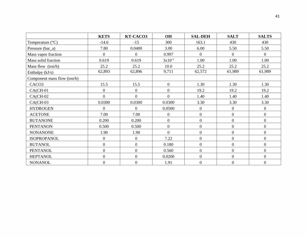
Table 4-8. Ketonization mass and heat balance

ALCOHOL CACO3 H2 H2-1 H21 KET KET-CACO KETO KETONES

40

ALCOHOL CACO3 H2 H2-1 H21 KET KET-CACO KETO KETONES

Temperature (°C) 130 130 43 130 961 130 430 133 130

Pressure (bar_a) 55.0 7.60 0.900 54.8 55.0 7.60 0.0400 55.0 7.60

Mass vapor fraction 0.0190 0 1.00 1.00 1.00 0 0.38 0 0

Mass solid fraction 3x10-3 1.00 0 0 0 0.619 0.619 3x10-3 3x10-3

Mass flow (ton/h) 10 15.5 0.340 0.340 0.340 25.2 25.2 9.6 9.6

Enthalpy (kJ/s) 12,226 51,675 24 142 1,640 61,455 57,409 9,754 9,779


CACO3 0 15.5 0 0 0 15.5 15.5 0 0

CA(CH-03) 0.0300 0 0 0 0 0.0300 0.0300 0.0300 0.0300

HYDROGEN 0.0500 0 0.340 0.340 0.340 0 0 0 0

ACETONE 0 0 0 0 0 7.00 7.00 7.00 7.00

BUTANONE 0 0 0 0 0 0.200 0.200 0.200 0.200

HEXANONE 0 0 0 0 0 0 0 0 0

PENTANON 0 0 0 0 0 0.500 0.500 0.500 0.500

HEPTANON 0 0 0 0 0 0 0 0 0

NONANONE 0 0 0 0 0 1.90 1.90 1.90 1.90

ISOPROPANOL 7.20 0 0 0 0 0 0 0 0

BUTANOL 0.180 0 0 0 0 0 0 0 0

HEXANOL 2x10-3 0 0 0 0 0 0 0 0

PENTANOL 0.560 0 0 0 0 0 0 0 0

HEPTANOL 0.0100 0 0 0 0 0 0 0 0

NONANOL 1.90 0 0 0 0 0 0 0 0


41

KETS KT-CACO3 OH SAL-DEH SALT SALTS

Temperature (°C) -14.6 -15 300 163.1 430 430

Pressure (bar_a) 7.80 0.0400 3.00 6.00 5.50 5.50

Mass vapor fraction 0 0 0.997 0 0 0

Mass solid fraction 0.619 0.619 3x10-3 1.00 1.00 1.00

Mass flow (ton/h) 25.2 25.2 10.0 25.2 25.2 25.2

Enthalpy (kJ/s) 62,893 62,896 9,711 62,572 61,989 61,989


CACO3 15.5 15.5 0 1.30 1.30 1.30

CA(CH-01 0 0 0 19.2 19.2 19.2

CA(CH-02 0 0 0 1.40 1.40 1.40

CA(CH-03 0.0300 0.0300 0.0300 3.30 3.30 3.30

HYDROGEN 0 0 0.0500 0 0 0

ACETONE 7.00 7.00 0 0 0 0

BUTANONE 0.200 0.200 0 0 0 0

PENTANON 0.500 0.500 0 0 0 0

NONANONE 1.90 1.90 0 0 0 0

ISOPROPANOL 0 0 7.22 0 0 0

BUTANOL 0 0 0.180 0 0 0

PENTANOL 0 0 0.560 0 0 0

HEPTANOL 0 0 0.0200 0 0 0

NONANOL 0 0 1.91 0 0 0

42

Table 4-9. Heat balances for Ketonization equipments


Heater H-107 583 2.10x106

Heater H-108 905 3.26x106

Heater H-109 2,515 9.05x106

Cooler C-102 3,629 1.31x107

Cooler C-103 1,163 4.19x106

Pumps P-105 3.10 1.12x104

Pumps P-106 25.2 9.07x104

Compressor CM-103 1,281 4.61x106

Reactor R-107 4,580 1.65x107

Reactor R-108 -2,615 -9.41x106

- Lime kiln (Unit 5)

In LIME KIL block the calcium carbonate labeled as CACO3 that come from

KETONIZA block is divided in two streams: (i) the stream labeled as CACO3-2 with a

flow of 9.20 ton/h is converted into quick lime (CaO). And (ii) the second stream labeled as

CACO3-1 with a flow of 6.30 ton/h is recycled to a PRET-FER block for Fermentation

process as was explained in that block before. The lime kiln simulation is shown in Figure

4-7. The conversion factor for Equation 4-5 in the reactor R-109 is 1, with an

endohothermic enthalpy of 4,529 kJ/ (Gosseaume, 2011). Table 4-11 shows the mass and

heat balance of this process.

(Eq. 4-5)

43

Figure 4-7. Lime kiln simulation

Table 4-10. Heat balances for Lime kiln equipments


Cooler C-104 521 1.88x106

Heater H-110 987 3.55x106

Reactor R-109 4,529 1.63x107

44

Table 4-11. Lime kiln mass and heat balance

CACO3 CACO3-1 CACO3-2 CACO3-3 CAO CAO-CO2

Temperature (°C) 130 130 130 500 500 55.0

Pressure (bar_a) 7.60 7.60 7.60 1.00 1.00 1.00

Mass vapor fraction 0 0 0 0 0.440 0.440

Mass solid fraction 1.00 1.00 1.00 1.00 0.560 0.560

Mass flow (ton/h) 15.54 6.3 9.24 9.24 9.24 9.24

Enthalpy (kJ/s) 51,675 20,949 30,725 29,738 25,209 26,310


CO2 0 0 0 0 4.06 4.06

CACO3 15.54 6.30 9.24 9.24 0 0

CAO 0 0 0 0 5.18 5.18

- Final (Unit 6)

The final block includes the mixed alcohols (stream labeled as OH in Figure 4-8)

conversion produce hydrocarbon fuels by alcohols dehydration olefins oligomerization

(product stream labeled as OLF-C9-12 in Figure 4-8) and olefin hydrogenation (product

stream labeled as PARAFIN in Figure 4-8). The final block simulation is shown in Figure

4-8.

The alcohols dehydration from stream labeled OH to produced 7.30 ton/h of olefins C3

to C9 stream labeled as OLF-C3-9 in Figure 4-8, occurred in reactor R-110, where the

conversion factor is 1 for the reactions shown in Appendix A (Eq. A-23 to A-28)

(Gosseaume, 2011). The heat duty for an endothermic reaction is 1,892kJ/s (Table 4-13).

The olefins produced in R-110 goes to a Oligomerization process to produced 7.30

ton/h of olefins C3 to C12 stream labeled as OLF-C3-12 in Figure 4-8, these reactions were

present in reactor R-111. In Table A-2 (Appendix A) are shown the conversion factors for

45

reactions by the Equations A-29 to A-36.The heat duty for an exothermic reaction is -

1,645kJ/s (Table 4-13).

To improve fuel quality, the olefins labeled as OLEFIN in Figure 4-8 were

hydrogenated to make 7.30 ton/h of corresponding paraffins (stream labeled as PARAFIN

in Figure 4-8) in reactor R-112, where the conversion factor is 1 (Gosseaume, 2011).

Olefin hydrogenation reactions are presented in Equations A-37 to A-45 (Appendix A).

And the heat duty for an exothermic reaction is -2,421kJ/s (Table 4-13). In this block, the

net demand of hydrogen is 0.0190 ton H2/ton hydrocarbon fuels; this hydrogen is produced

in gasification block explained in the next section.

Finally, the hydrocarbon fuel labeled as HC in Figure 4-8 is distilled into C8- and C9+

fractions. The light fraction and the heavy fraction can be used as blending components for

gasoline and jet fuel, respectively, as Pham et al., (2012) mentioned. A ratio of 53 gallons

of light fraction per ton of biomass is obtained for a total of 2,127 gallon/h of gasoline. And

for heavy fraction the ratio is 19 gallons per ton of biomass for a total of 762 gallon/h of jet.

Table 4-12 shows the material balance of the entire block. On the other hand, heat

balances for this block shows a power consumption of 997 kW for compressor CM-104 and

CM-105 (Table 4-13). The cooling demand in this block is 4,470kJ/s and the heating

demand is 1,536kJ/s.

Figure 4-9 shows a comparison between the gasoline obtained by MixAlco® and a

mixture of light naphtha (LVN) and gases fossil fuel consulted in an article of Cartagena

refinery (Fernández, 2007). The gasoline curve obtained by MixAlco® had a similar

behavior of LVN except for gas fraction.

46

Figure 4-8. Final simulation

Table 4-12. Final mass and heat balance

C3 H2 H2- H2-1 H20 HC HC-C4--8 HC-C9-12 HEAVY LIGHT

Temperature (°C) 130 43 961 130 300 130 266 408 25 25

Pressure (bar_a) 55.0 0.900 55.0 55.0 3.00 55.0 50.0 53.0 1.00 1.00

Mass vapor fraction 0.770 1.00 1.00 1.00 1.00 0 0 0 0 0

Mass solid fraction 0.230 0 0 0 0 0 0 0 0 0

Mass flow (ton/h) 0.130 0.100 0.100 0.100 2.60 7.40 5.30 2.10 2.10 5.30

Enthalpy (kJ/s) 32.0 7.97 537 537 9.17 4.04 2,081 481 1,228 3,382


47

C3 H2 H2- H2-1 H20 HC HC-C4--8 HC-C9-12 HEAVY LIGHT

WATER 0 0 0 0 2.60 0 0 0 0 0

CA(CH-03 0.0300 0 0 0 0 0 0 0 0 0

HYDROGEN 0 0.100 0.100 0.100 0 0 0 0 0 0

C3H6 0.100 0 0 0 0 0 0 0 0 0

C4H10 0 0 0 0 0 0.0900 0.0900 0 0 0.0900

C5H12 0 0 0 0 0 0.200 0.20 0 0 0.200

C6H14 0 0 0 0 0 4.73 4.73 0 0 4.73

C7H16 0 0 0 0 0 0.0300 0.0300 0 0 0.0300

C8H18 0 0 0 0 0 0.230 0.230 0 0 0.230

C9H20 0 0 0 0 0 1.41 0 1.41 1.41 0

C10H22 0 0 0 0 0 0.0400 0 0.0400 0.0400 0

C11H24 0 0 0 0 0 0.190 0 0.190 0.190 0

C12H26 0 0 0 0 0 0.450 0 0.450 0.450 0


OH OLEFIN OLF OLF-C3-9 OLF-DEH OLFC3-12 PARAFIN

Temperature (°C) 300 130 399.9 300 300 300 130

Pressure (bar_a) 3.00 54.5 55.0 3.00 3.00 3.00 55.0

Mass vapor fraction 0.997 0.0390 0.996 0.997 0.996 0.997 7x10-3

Mass solid fraction 3x10-3 4x10-3 4x10-3 3x10-3 4x10-3 3x10-3 4x10-3

Mass flow (ton/h) 10.0 7.40 7.40 10.0 7.40 10.0 7.50

Enthalpy (kJ/s) 9,711 1,699 287 7,819 289 9,464 4,073


WATER 0 0 0 2.56 0 2.56 0

CA(CH-03 0.030 0.030 0.030 0.030 0.030 0.030 0.030

48

OH OLEFIN OLF OLF-C3-9 OLF-DEH OLFC3-12 PARAFIN

HYDROGEN 0.050 0.050 0.050 0.050 0.050 0.050 0.010

ISOPROPANOL 7.22 0 0 0 0 0 0

BUTANOL 0.180 0 0 0 0 0 0

HEXANOL 0 0 0 0 0 0 0

PENTANOL 0.560 0 0 0 0 0 0

HEPTANOL 0.0200 0 0 0 0 0 0

NONANOL 1.91 0 0 0 0 0 0

C3H6 0 0.100 0.100 5.05 0.100 0.100 0.101

C4H8 0 0.0900 0.0900 0.140 0.0900 0.0900 0

C5H10 0 0.190 0.190 0.450 0.190 0.190 0

C6H12 0 4.62 4.62 0.00 4.62 4.62 0

C7H14 0 0.0300 0.0300 0.0100 0.0300 0.0300 0

C9H18 0 1.38 1.38 1.67 1.38 1.38 0

C8H16 0 0.230 0.230 0 0.230 0.230 0

C10H20 0 0.0400 0.0400 0 0.0400 0.0400 0

C11H22 0 0.180 0.180 0 0.180 0.180 0

C12H24 0 0.450 0.450 0 0.450 0.450 0

C4H10 0 0 0 0 0 0 0.0900

C5H12 0 0 0 0 0 0 0.200

C6H14 0 0 0 0 0 0 4.73

C7H16 0 0 0 0 0 0 0.0300

C8H18 0 0 0 0 0 0 0.230

C9H20 0 0 0 0 0 0 1.41

C10H22 0 0 0 0 0 0 0.0400

C11H24 0 0 0 0 0 0 0.190

C12H26 0 0 0 0 0 0 0.450

49

Table 4-13. Heat balances for Final equipments


Heater Reboiler T-101 1,536 5.53x106

Cooler C-105 381 1.37x106

Cooler C-106 1,987 7.15x106

Cooler C-107 1,301 4.68x106

Cooler C-108 746 2.69x106

Cooler Condenser T-101 54.6 1.97x105

Compressor CM-104 577 2.08x106

Compressor CM-105 420 1.51x106

Reactor R-110 1,893 6.81x106

Reactor R-111 -1,645 -5.92x106

Reactor R-112 -2,421 -8.72x106

Figure 4-91. Distillation curve for gasoline

Figure 4-10 shows a comparison between the jet obtained by MixAlco® and jet

fossil fuel consulted in an article of Cartagena refinery (Fernández, 2007). The jet curve

50

obtained by MixAlco® had a similar behavior of jet fossil fuel except for the final

temperature, where the jet in MixAlco® is lighter for about 56.0°C.

Figure 4-10. Distillation curve for Jet

- Gasification (Unit 7)

The last block in MixAlco® process is GASIFICA shown in Figure 4-11. All hydrogen

demand in MixAlco® process is obtained in this block. In reactor R-113 is simulated the

gasification of biomass undigested that come from pretreatment (stream labeled as BIO-

PRET in Figure 4-11) and fermentation (stream labeled as BIOM-FER in Figure 4-11)

process and is converted to hydrogen (stream labeled as BM-C-H2O) for a production of

0.200 ton/h. The conversion factor for reactions Eq. 4-6 and 4-7 are 0.280 and 0.680,

respectively (Gosseaume, 2011). Also, it is produced 3.20 ton/h of CO, 8.00 ton/h of CO2

and 3.10 ton/h of water. The vapor obtained in gasification is separated in S-107 to the

char; where the obtained gas is called as SYNGAS. In order to use the heat duty of this gas

a power generation is installed producing a work of 1,180 kW from the turbine TR-101.

51

Figure 4-11. Gasification simulation

After power generation, the syngas produce more hydrogen (0.250 ton/h) by the steam-gas shift reactor (R-114), the conversion

factor for Equation 4-8 is 1 (Gosseaume, 2011). Table 4-14 shows the mass balance for this block. Table 4-15 show the heat balances

for the equipment, where a power demand is 28.7 kW for pump P-107, the cooling demand is 5.07 kJ/s, and the exothermic duty is

10,555kJ/s for reactor R-113 and R-114.

(Eq. 4-6)

(Eq. 4-7)

(Eq. 4-8)

52

Table 4-14. Gasification mass and heat balance

BIO BIO-PRET BIOM BIOMAS BM-C-H2O C+H2+H20 CHAR CO2 GAS H2 H2+

Temperature (°C) 55.0 55.0 55.0 55.0 760 254 760 43.0 254 43.0 43.0

Pressure (bar_a) 1.00 1.00 1.00 1.00 1.00 1.00 1.00 0.900 0.800 0.900 0.900

Mass vapor fraction 0.500 0 0 0.500 0.900 1.00 0 1.00 1.00 1.00 1.00

Mass solid fraction 0.500 0.0200 1.00 0.500 0.100 0 1.00 0 0 0 0

Mass flow (ton/h) 24.8 432 8.70 16.1 31.6 22.8 8.8 20.9 22.8 0.5 22.8

Enthalpy (kJ/s) 46,334 1,854,269 20,498 46,334 55,629 54,051 7,359 51,803 52,791 32.28 55,749


CELLU-01 3.80 2.80 2.80 1 3.80 0 3.8 0 0 0 0

XYLAN 3.10 2.80 2.80 0.400 3.10 0 3.1 0 0 0 0

LIGNI-01 10.1 3.20 3.20 6.90 1.90 0 1.9 0 0 0 0

SOLSL-01 0 5 0 0 0 0 0 0 0 0 0

SOLUN-01 0 0 0 0 0 0 0 0 0 0 0

WATER 0 418 0 0 3.10 1.07 0 0 3.10 0 1.10

AIR 0 0 0 0 0 0 0 0 0 0 0

CO 0 0 0 0 3.20 0 0 0 3.20 0 0

CO2 7.80 0 0 7.80 15.8 20.9 0 20.9 15.8 0 20.9

O2 0 0 0 0 0.400 0.400 0 0 0.400 0 0.400

HYDROGEN 0 0 0 0 0.200 0.500 0 0 0.200 0.500 0.500


H2O+02 H20 LIQSAT O2 O2+H20 STEAMSAT STEAMSUP SYNGAS WAT WATER

Temperature (°C) 43.0 95.0 90.0 25.0 43.0 162 577 760 55.0 95.0

Pressure (bar_a) 0.900 63.0 0.800 1.00 0.900 1.00 62.0 1.00 1.00 63.0

Mass vapor fraction 0.900 0 0 1.00 0.300 1.00 1.00 1.00 0 0

Mass solid fraction 0 0 0 0 0 0 0 0 0 0

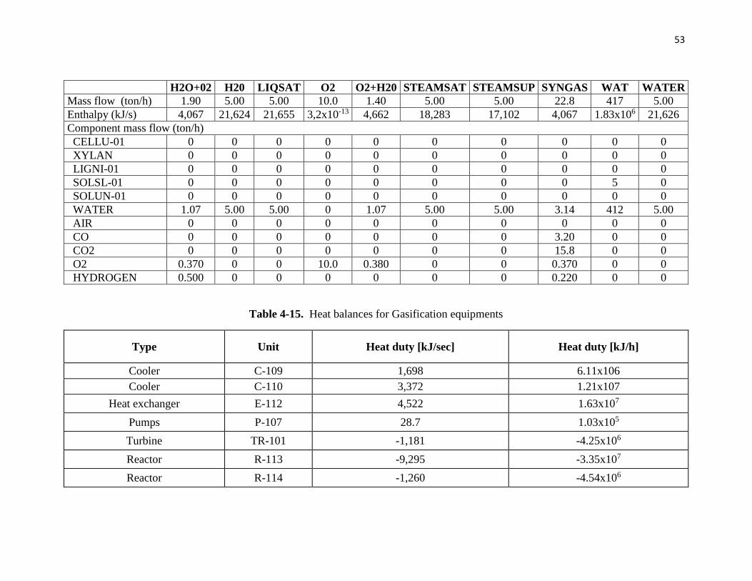
53

H2O+02 H20 LIQSAT O2 O2+H20 STEAMSAT STEAMSUP SYNGAS WAT WATER

Mass flow (ton/h) 1.90 5.00 5.00 10.0 1.40 5.00 5.00 22.8 417 5.00

Enthalpy (kJ/s) 4,067 21,624 21,655 3,2x10-13 4,662 18,283 17,102 4,067 1.83x106 21,626


CELLU-01 0 0 0 0 0 0 0 0 0 0

XYLAN 0 0 0 0 0 0 0 0 0 0

LIGNI-01 0 0 0 0 0 0 0 0 0 0

SOLSL-01 0 0 0 0 0 0 0 0 5 0

SOLUN-01 0 0 0 0 0 0 0 0 0 0

WATER 1.07 5.00 5.00 0 1.07 5.00 5.00 3.14 412 5.00

AIR 0 0 0 0 0 0 0 0 0 0

CO 0 0 0 0 0 0 0 3.20 0 0

CO2 0 0 0 0 0 0 0 15.8 0 0

O2 0.370 0 0 10.0 0.380 0 0 0.370 0 0

HYDROGEN 0.500 0 0 0 0 0 0 0.220 0 0

Table 4-15. Heat balances for Gasification equipments


Cooler C-109 1,698 6.11x106

Cooler C-110 3,372 1.21x107

Heat exchanger E-112 4,522 1.63x107

Pumps P-107 28.7 1.03x105

Turbine TR-101 -1,181 -4.25x106

Reactor R-113 -9,295 -3.35x107

Reactor R-114 -1,260 -4.54x106

54

4.1.1.2 MixAlco® overall mass balance results

In numeral 3.1.1.1 was described mass and heat balances for MixAlco® process. Table 4-16 summarized some relations

discussed in that numeral. The theoretical relations helps to verified that results obtained in the simulation are according to the

literature review. The sources consulting for these relations are: (Pham et al., 2010), (Sierra et al., 2010), (Holtzapple, 2004),

(Gosseaume, 2011).

Table 4-16. MixAlco® yields

Unit Parameter Value Calculated relations Theoretical relations

Feed

Handling

Biomass feed (ton/h) 40.0

CaO feed Total (ton/h) 6.07 0.150 Total ton CaO/ton Biomass 0.150 Total g CaO/g Biomass

CaO feed recycle (ton/h) 5.17 0.127 ton CaO recycle /ton Biomass

CaO feed make up (ton/h) 0.900 0.0225 ton CaO Make up /ton Biomass 0.0230 g CaO Make up /g Biomass

H2O to Feed-Handling (ton/h) 2.00 0.0500 ton H2O Make up /ton Biomass

Ca(OH)2 Production (ton/h) 7.90 0.200 ton Ca(CHO)2 /ton Biomass

Pretreatment

Cellulose digested (ton/h) 14.3 85.0% of Cellulose inlet 85.0% of Cellulose inlet

Xylan digested (ton/h) 4.90 65.0% of xylan inlet 65.0% of xylan inlet

Lingni digested (ton/h) 7.00 70.0% of lingni inlet 70.0% of lingni inlet

Volatile solid = biomass VS (ton/h) 34.3 0.800 ton biomass VS / ton Biomass

Conversion Biomass digested (ton/h) 26.2 0.800 ton digested / ton biomass VS 0.800 g digested / g volatile solid fed

Biomass undigested (ton/h) 8.10 0.200 ton undigested / ton biomass VS 0.200 ton undigested / ton biomass VS

Air consumption (ton/h) 6.70 0.170 ton Air /ton Biomass

H2O to pretreatment (ton/h) 400 10.0 ton H2O /ton Biomass 5.00 to 15.00 ton H2O /ton Biomass

Reaction time (week / days) (6/42) (6 / 42)

Fermentation Carboxylate salts (ton/h) 24.0 0.60ton carboxylate salts / ton Biomass 0.600 ton carboxylate salts / ton Biomass

55


Volatile fatty acid (VFA) (ton/h) 19.0 1.26 ton salt / ton VFA

Selectivy 0.700 ton VFA / ton digested

0.650 g carboxylic acids / g volatile solids

digested

Mixed acid yield 0.600 ton VFA / ton biomass VS 0.520 ton VFA / ton biomass VS

H2O to fermentation (ton/h) 200 5.00 ton H2O /ton Biomass 5.00 ton H2O /ton Biomass

CaCO3 total (ton/h) 14.3 0.400 Total ton CaCO3 /ton Biomass 0.400 Total ton CaCO3 /ton Biomass

CO2 produced (ton/h) 7.80 0.200 ton CO2 /ton Biomass 0.200 ton CO2 /ton Biomass

Reaction time (week / days) (8/56)

(8 / 56)

Ketonization CaCO3 production (ton/h) 14.2 0.360 ton CaCO3 /ton Biomass 0.360 ton CaCO3 /ton Biomass

Ketones (ton/h) 9.60 0.510 ton ketones/ ton VFA 0.510 g ketones/ g carboxylic acids

Ketone

Hydrogenatio

n

Alcohols (ton /h) 9.87 0.520 ton alcohol / ton VFA 0.520 ton alcohol / ton VFA

0.250 ton alcohol / ton Biomass 0.250 ton alcohol / ton Biomass

H2 consumption (ton /h) 0.287 0.0290 ton H2 demand / ton alcohol 0.0225 kg H2 / kg mixed alcohol

0.00700 ton H2 demand / ton Biomass 0.00687 kg H2 demand / kg Biomass

Lime kiln

CaCO3 to lime kiln (ton/h) 9.20

CaCO3 to fermentation (ton/h) 6.30

CaO for recycle to feed handling

(ton/h) 5.20

Alcohol

Dehydration

Olefins (ton/h) 7.30 0.180 ton Olefin / ton Biomass

H2O produced (ton/h) 2.56 0.350 ton H2O produced / ton Olefin

Olefin

hydrogenatio

n

Parafins (ton/h) 7.37

H2 consumption (ton /h) 0.140 0.0190 ton H2 demand / ton Parafin 0.0139 kg H2 / kg hydrocarbon fuels

0.00350 ton H2 demand / ton Biomass 0.00340 kg H2 demand / kg Biomass

Final

Light hydrocarbon (C8-) (ton/h) 5.28

0.400 g Light hydrocarbon yield /g

alcohol 0.600 g Light hydrocarbon yield /g alcohol

Heavy hydrocarbon (C9+) (ton/h) 2.09

0.200 g Heavy hydrocarbon yield /g

alcohol 0.200 g Heavy hydrocarbon yield /g alcohol

Light hydrocarbon (gallon/h) 2127 53 gallons Light hydrocarbon /ton Biomass 62.0 gallons Light hydrocarbon /ton Biomass

56


Heavy hydrocarbon (gallon/h) 762

19 gallons Heavy hydrocarbon /ton

Biomass 19.0 gallons Heavy hydrocarbon /ton Biomass

Gasification

& Steam-gas

shift

H2 produced in gasification (ton/h) 0.200

H2 produced in Steam-gas shift

(ton/h) 0.250

4.1.1.3 MixAlco® overall heat balance results

Table 4-17 shows a summary of heat balances for the equipment simulated in MixAlco® process, where the total heating

demand is 120,288 kJ/s (4.33x108 kJ/h). Also, the total cooling demand is 22,809 kJ/s (8.21x107 kJ/h); The total power required for

pumps and compressors, without the power generated in the turbine TR-101 by the gasification process is 2,408 kJ/s (8.67x106 kJ/h).

Table 4-17. Summary fo heat balances for MixAlco® processs

HEATERS COOLERS PUMPS COMPRESSORS REACTORS HEAT

EXCHANGERS

Feed handling (kJ/s) -1,541

Pretreatment & Fermentation (kJ/s) 7,957 30.0 10 18,427

Dewatering (kJ/s) 113,762 1,215 143,451

Ketonization & Lime kiln (kJ/s) 4,990 5,313 28.0 1,281 6,494

Final (kJ/s) 1,536 4,470 997 -2,174

Gasification (kJ/s) 5,070 28.0 -1,181 -10,555 4,522

Total heat duty (kJ/s) 120,288 22,809 87.0 2,323 10,651 147,973

Total heat duty (kJ/h) 4.33x108 8.21x107 3.11x105 8.36x106 3.83x107 5.33x108

57

Actual heat integration has a heat exchangers duty of 147,973 kJ/s (5.33x108kJ/h). In Table 4-17, heat duty with negative

signal stands for exothermic reactions, meanwhile positive stands for endothermic reactions.

4.1.2 Simulation build up and results for CODP base case

The CODP simulation was divided in four blocks to build up a simulation: two preheating trains, one atmospheric distillation

unit and one vacuum distillation unit. The blocks are shown in Figure 4-12.

Figure 4-12. Blocks of CODP simulation

58

4.1.2.1 CODP Block description

- First preheating train

Figure 4-13. First pre-heating train

59

The crude oil (named CRUDE-IN) was feed to the first preheating train at 30.6°C

and 2.4bar_a. Figure 4-13 shows this process. This train was heat integrated with side

stream OVHT204 from the atmospheric distillation, and with the second preheating train by

the stream DIE203. The target was to heat the crude oil at 183.5°C before enter to the

second preheating train. This stream (fed stream of the second preheating train) was named

CRDTP1.

Table 4-18 shows the mass balance obtained for this process. On the other hand,

Table 4-19 shows the heat balances for this block, where exist a cooling demand of

1.59x107 kJ/s for the cooler (C-201) plus the flash separator (SP-201); in this block did not

exist heaters. The power required for pumps are 0.21MW.

Table 4-18. First train preheating mass and heat balance

CRD-IN CRDE201 CRDE203 CRDTP1 CRUDE-IN DIE203

Temperature (°C) 31.8 127 183 183 30.6 236

Pressure (bar_a) 26.9 26.9 25.8 27.1 2.40 9.00

Mass vapor fraction 0 0 0 0 0 0

Mass flow (ton/h) 162 162 162 162 162 88.0

Enthalpy (kJ/s) 83,851 75,245 69,430 69,430 84,083 32,447


WATER 0 0 0 0 0 0

ETHANE 0 0 0 0 0 0

PROPANE 0.100 0.100 0.100 0.100 0.100 0

ISOBUTANE 0.100 0.100 0.100 0.100 0.100 0

N-BUTANE 0.200 0.200 0.200 0.200 0.200 0

ISOPENTANE 0.400 0.400 0.400 0.400 0.400 0

N-PENTANE 0.400 0.400 0.400 0.400 0.400 0

N-HEXANE 0.400 0.400 0.400 0.400 0.400 0

PSEUDOCOMPONENTS 160.4 160.4 160.4 160.4 160.4 87.7

60


DIEST204 DIEST204 GAST204 MPAT204 OVH201

Temperature (°C) 137.8 137.8 0 137.8 99.8

Pressure (bar_a) 9.60 9.60 1.70 9.60 2.00

Mass vapor fraction 0 0 0 0 0.088

Mass flow (ton/h) 88.0 88.0 0 52.8 64.8

Enthalpy (kJ/s) 15,351 38,378 0 23,027 46,635


WATER 0 0 0 0 3.90

PROPANE 0 0 0 0 0.100

ISOBUTANE 0 0 0 0 0.100

N-BUTANE 0 0 0 0 0.300

ISOPENTANE 0 0 0 0 0.500

N-PENTANE 0 0 0 0 0.600

N-HEXANE 0 0 0 0 1.00

PSEUDOCOMPONENTS 87.7 87.7 0 52.5 58.2

Table 4-19. Heat balances for equipments in 1st preheating train

Type Unit Heat duty

[kJ/sec]

Heat duty

[kJ/h]

Exchanger

area [m2]

Cooler C-201 3,056 1.10x107 NA

Heat exchanger E-201 8,595 3.09x107 271


Flash separator SP-201 1,352 4.87x106

Pump P-201 200 7.20x105

Pump P-202 10 3.60x104

- Second preheating train

The second preheating train was fed with the stream CRDTP1, which was at 183.5°C

and 27.1 bar_a. Figure 4-14 shows, this process. As the first preheating train, this train was

heat integrated with side stream DIEST-04 from the atmospheric distillation, and with side

streams ASPAHLT and HVGO-205 from the vacuum distillation The target was to take the

CRDTP1 stream conditions to 277.2°C (atmospheric tower conditions).

61

The resulting stream from this train was named CRDT204. Table 4-20 shows the mass balance of this process. On the other

hand, Table 4-21 shows the energy balances for this block, where exist a cooling demand of 9.25x106 kJ/s for the cooler (C-202); in

this block did not exist heaters.

Figure 4-14. Second pre-heating train

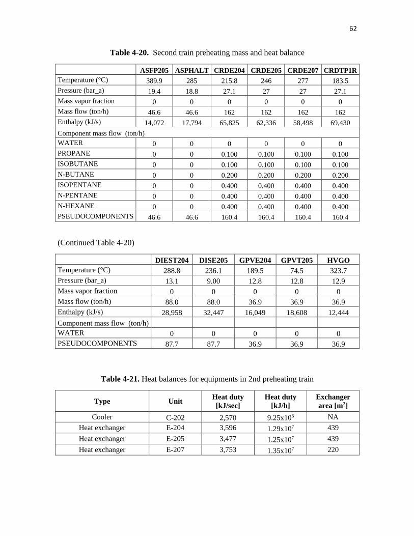
62

Table 4-20. Second train preheating mass and heat balance

ASFP205 ASPHALT CRDE204 CRDE205 CRDE207 CRDTP1R

Temperature (°C) 389.9 285 215.8 246 277 183.5

Pressure (bar_a) 19.4 18.8 27.1 27 27 27.1

Mass vapor fraction 0 0 0 0 0 0

Mass flow (ton/h) 46.6 46.6 162 162 162 162

Enthalpy (kJ/s) 14,072 17,794 65,825 62,336 58,498 69,430


WATER 0 0 0 0 0 0

PROPANE 0 0 0.100 0.100 0.100 0.100

ISOBUTANE 0 0 0.100 0.100 0.100 0.100

N-BUTANE 0 0 0.200 0.200 0.200 0.200

ISOPENTANE 0 0 0.400 0.400 0.400 0.400

N-PENTANE 0 0 0.400 0.400 0.400 0.400

N-HEXANE 0 0 0.400 0.400 0.400 0.400

PSEUDOCOMPONENTS 46.6 46.6 160.4 160.4 160.4 160.4


DIEST204 DISE205 GPVE204 GPVT205 HVGO

Temperature (°C) 288.8 236.1 189.5 74.5 323.7

Pressure (bar_a) 13.1 9.00 12.8 12.8 12.9

Mass vapor fraction 0 0 0 0 0

Mass flow (ton/h) 88.0 88.0 36.9 36.9 36.9

Enthalpy (kJ/s) 28,958 32,447 16,049 18,608 12,444


WATER 0 0 0 0 0

PSEUDOCOMPONENTS 87.7 87.7 36.9 36.9 36.9

Table 4-21. Heat balances for equipments in 2nd preheating train

Type Unit Heat duty

[kJ/sec]

Heat duty

[kJ/h]

Exchanger

area [m2]

Cooler C-202 2,570 9.25x106 NA




63

- Atmospheric distillation unit

The atmospheric distillation unit is shown in Figure 4-15. The atmospheric distillation column (named T-204) is considered the

master unit, because different cuts of the oil crude were obtained. This column had one stripper, two pumparounds, furnace and

condenser. The components of the feed stream were separated as: gas, naphtha, jet, diesel, gas oils and atmospheric residues.

Figure 4-15. Atmospheric distillation column

64

Due to the large amount of heat duty from gas and diesel product streams, those were heating integrated with the first and

second preheating trains. Table 4-22 shows the mass balance. The crude oil named (CRDPREC) fed this tower, which was at 277.2°C

and 27.1 bar_a. The yields obtained in this unit are shown in numeral 5.1.2.2 Table 4-23 shows the energy balances for this block,

where exist a cooling demand of 6.86x107 kJ/s for the cooler (C-203), the condenser, the pumparounds and the separators; the total

heating demand is 9.64x107 kJ/s for the heater (H-201) and the furnace. The power demands for pumps are 0.0230 MW.

Table 4-22. Atmospheric distillation mass and heat balance

AGOP204 AGOT204 CRDH202 CRDPREC DIEM201 DIEST204 GAS-S203 GAST4 JET-T204 JETP203

Temperature (°C) 358.3 357 226.9 277.2 288.8 304 98.3 97.8 69.5 194.4

Pressure (bar_a) 12.9 2.20 19.1 27.0 13.1 2.20 1.70 1.70 13.9 13.9

Mass vapor fraction 0 0 0 0 0 0 1.00 1.00 0 0

Mass flow (ton/h) 6.40 6.40 162 162 88.0 35.0 0 11.2 19.8 19.8

Enthalpy (kJ/s) 1,861 1,977 64,545 58,498 28,958 11,397 0 11,979 9,304 7,676


WATER 0 0 0 0 0 0 0 2.10 0 0

PROPANE 0 0 0.100 0.100 0 0 0 0.100 0 0

ISOBUTANE 0 0 0.100 0.100 0 0 0 0.100 0 0

N-BUTANE 0 0 0.200 0.200 0 0 0 0.200 0 0

ISOPENTANE 0 0 0.400 0.400 0 0 0 0.400 0 0

N-PENTANE 0 0 0.400 0.400 0 0 0 0.300 0 0

N-HEXANE 0 0 0.400 0.400 0 0 0 0.400 0 0

PSEUDOCOMPONENTS 6.20 6.20 160.4 160.4 87.7 35.0 0 7.70 19.8 19.8

65


JETT204 LIGNAPH MPAM201 MPAT204 NAPHT204 OVHT204 RESIDUE STEAM-4 STEAM-JT WATSP203

Temperature (°C) 193.5 98.3 278.9 147.7 97.8 144.4 365.6 352.8 353.3 98.3

Pressure (bar_a) 2.90 1.70 2.20 2.20 1.70 2.20 2.20 5.10 5.10 1.70

Mass vapor fraction 0 0 0 0 0 1.00 0 1.00 1.00 0

Mass flow (ton/h) 19.8 2.60 52.9 52.9 4.40 64.8 88.7 3.20 0.600 1.60

Enthalpy (kJ/s) 7,676 1,396 17,561 22,562 8,373 38,029 27,563 11,281 2,093 6,978


WATER 0 0 0 0 1.60 3.90 0 3.20 0.600 1.60

PROPANE 0 0 0 0 0 0.10 0 0 0 0

ISOBUTANE 0 0 0 0 0 0.10 0 0 0 0

N-BUTANE 0 0 0 0 0 0.30 0 0 0 0

ISOPENTANE 0 0 0 0 0 0.50 0 0 0 0

N-PENTANE 0 0 0 0 0 0.60 0 0 0 0

N-HEXANE 0 0 0 0 0 1.00 0 0 0 0

PSEUDOCOMPONENTS 19.8 2.60 52.9 52.9 2.70 58.2 88.7 0 0 0

Table 4-23. Heat balances for equipment in atmospheric distillation unit

Type Unit Heat duty [kJ/sec] Heat duty

[kJ/h]

Heater H-201 4,922 1.77x107

Heater Furnace 21,848 7.87x107

Cooler C-203 1,614 5.81x106

Cooler Condenser 5,774 2.08x107

Cooler Pumparound MPA 5,113 1.84x107

Cooler Pumparound MPACAL 563 2.03x106


Flash separator SP-203 10.0 3.60x104

Pump P-203 16.0 5.76x104

Pump P-204 7.00 2.52x104

66

- Vacuum distillation unit

The vacuum distillation unit is shown in Figure 4-16. In the vacuum distillation column (named T-205), the crude oil was fed

with the bottom stream of T-204. In order to prevent the breakdown of the reduced crude, this unit worked at high temperatures

and vacuum pressure. The obtained cuts were: gas, light gas oil, heavy gas oil, and vacuum residue. Due to the large amount of

heat duty from HVGOT205 and ASPHALT product streams, those were heating integrated with the second preheating train.

Figure 4-16. Vacuum distillation column

67

Table 4-24 shows the mass balance obtained for this unit. The crude oil named (CRDT204) fed this tower, which was at

365.6°C and 2.2 bar_a. The yields obtained in this unit are shown in numeral 5.1.2.2. Table 4-25 shows the energy balances for this

block, where exist a cooling demand of 3.99x107 kJ/s for the cooler (C-204), the condenser, the pumparounds and the separators; the

total heating demand is 2.44x107 kJ/s for the heater (H-202). The power demand for the pump P-205 is 0.0480 MW.

Table 4-24. Vacuum distillation mass and heat balance

AGO ASPHALT ASPHP205 CRDH202 CRDT204 CREDT205 GAS-S204

Temperature (°C) 48.9 388.7 389.9 365.6 365.6 432.2

Pressure (bar_a) 1.20 0.100 19.4 1.00 2.20 0.100 1.20

Mass vapor fraction 0 0 0 0 0 0.590

Mass flow (ton/h) 0 46.6 46.6 88.8 88.8 88.8 0

Enthalpy (kJ/s) 0 14,072 14,072 27,563 27,563 20,817 0


PSEUDOCOMPONENTS 0 46.6 46.6 88.7 88.7 88.7 0

GPVM7 HVGOT205 LVGO-205 LVGOT205 OVHT205 STEAM-5 WAT-S204

Temperature (°C) 323.7 323.8 34.5 213.4 60 454.4 48.9

Pressure (bar_a) 12.9 0.100 10.2 0.100 0 3.70 1.20

Mass vapor fraction 0 0 0 0 1.00 1.00 0

Mass flow (ton/h) 36.9 36.9 5.30 5.30 3.00 3.00 3.00

Enthalpy (kJ/s) 12,444 12,444 2,675 2,210 11,165 10,467 13,142


WATER 0 0 0 0 3.00 3.00 3.00

PSEUDOCOMPONENTS 36.9 36.9 5.30 5.30 0 0 0

68

Table 4-25. Heat balances for equipments in vacuum distillation unit

Type Unit Heat duty

[kJ/sec] Heat duty [kJ/h]

Heater H-202 6,780 2.44x107

Cooler C-204 567 2.04x106

Cooler Condenser 308 1.11x106

Cooler Pumparound UPA 2,117 7.62x106

Cooler Pumparound MPA 5,874 2.11x107

Cooler Pumparound MPACAL 219 7.88x105


Pump P-205 48.0 1.73x105

4.1.2.2 CODP Overall mass balances results

Table 4-26 shows the yields for CODP. Defined yield as the mass ration between

refined products and the initial crude oil feed. A column pseudo-stream was used for

internal column calculations, but this pseudo-stream was not included in the column

material balance.

Table 4-26. COPD Yields


Atmospheric column

Yield (ton Naphta from T-204 /ton crude) 0.017

Yield (ton Jet from T-204 /ton crude) 0.123

Yield (ton Diesel from T-204 /ton crude) 0.217

Yield (ton AGO from T-204 /ton crude) 0.04

Vacuum column

Yield (ton LVGO from T-205 /ton crude) 0.033

Yield (ton HVGO from T-205 /ton crude) 0.228

Yield (ton VGO from T-205 /ton crude) 0

Yield (ton Asphalt from T-205 /ton crude) 0.287

69

4.1.2.3 CODP Overall heat balances results

Table 4-27 shows a summary of heat balances for equipments in CODP, the C

for separators means the needed heat is for cooling and the H is for heating. So, the total

heating utility is calculated as the duty for heaters plus the heat needed in separators with a

total duty of 1.26x108 kJ/s. Likewise, the total cooling utility is calculated with the coolers

duties plus the cooling duty needed in separators with a total duty of 1.29x108 kJ/s.

Table 4-27 also shows the heat exchangers used in CODP for the first and

second preheating trains. And the power required for pumps with a total power demand of

0.280 MW.

Table 4-273. Overall heat balances for CODP

HEATERS COOLERS PUMPS SEPARATORS HEAT EXCHANGERS

1-Train (kJ/s) 3,056 210 1,352 (C) 14,504

2-Train (kJ/s) 2,570 10,826

Atmospheric-unit (kJ/s) 26,770 13,064 23.0 5,982 (H)

Vacuum-unit (kJ/s) 6,780 9,085 48.0 2,011 (H)

Total heat duty (kJ/s) 33,550 27,775 281 9,345 25,330

Total heat duty (kJ/h) 1.21x108 1.00x108 1.01x106 3.36x107 9.12x107

4.2 Define needs

In this work, the need was defined as the technical-economical evaluation for a new

MixAlco® plant by retrofitting analysis with CODP, comparing with a base case (only a

new MixAlco® plant).

70

4.3 Retrofitting procedure applied: Process arrangements

4.3.1 Internal rearrangements

The first loop of the proposed methodology covers only internal arrangements. With

the aim of apply this first step, an improvement within each plant (MixAlco® and CODP)

with a mass and energy integration was proposed. This integration did not require any

addition of new equipment in each plant, according to the methodology.

4.3.1.1 MixAlco® process

- Mass integration

Appendix C shows a literature review of mass integration. In the base case,

MixAlco® process was using a mass integration of calcium carbonate between

ketonization, pretreatment, and fermentation units. In this integration, the byproduct stream

of calcium carbonate from ketonization is sent to fermentation unit as buffer salt. The

remaining amount is treated in a lime kiln to produce quick lime, needed in the

pretreatment process. Regardless, it is necessary use a make up of these substances.

(Gosseaume, 2011). Tables 4-28 and 4-29 show the mass balances obtained for fresh and

waste streams in the simulation.

71

Table 4-28. Fresh MixAlco® streams

Process FEED HANDLING PRETREATMENT FERMENTATION GASIFICATION

Stream Name H2O-LIME CAO-MAKE BIOMASS H20-PRET AIR H20-FERM MK-CACO3 O2 WATER

Temperature (°C) 25.0 55.0 25.0 25.0 25.0 50.0 25.0 25.0 95.0

Pressure (bar_a) 1.00 1.00 1.00 1.00 1.00 1.00 1.00 1.00 63.0

Mass Vapor Fraction 0 0 0 0 1.00 0 0 1.00 0

Mass Solid Fraction 0 1.00 0.870 0 0 0 1.00 0 0

Total mass flow (ton/h) 2.00 0.900 39.5 400 6.70 200 9.30 10.0 5.00


CELLU-01 0 0 16.8 0 0 0 0 0 0

XYLAN 0 0 7.50 0 0 0 0 0 0

LIGNI-01 0 0 10.0 0 0 0 0 0 0

SOLSL-01 0 0 5.17 0 0 0 0 0 0

WATER 2.00 0 0 400 0 200 0 0 5.00

CAO 0 0.900 0 0 0 0 0 0

CACO3 0 0 0 0 0 0 9.30 0 0

NITROGEN 0 0 0 0 5.30 0 0 0 0

O2 0 0 0 0 1.40 0 0 10.0 0

72

Table 4-29. Waste MixAlco® streams

Process DEWATERING FINAL GASIFICA

Stream Name WATDISTI H2O C3 WAT O2+H20 CHAR CO2

Temperature (°C) 60.0 300 130 55.0 43.0 760 43.0

Pressure (bar_a) 5.50 3.00 55.0 1.00 0.900 1.00 0.900

Mass Vapor Fraction 0 1.00 0.770 0 0.300 0 1.00

Mass Solid Fraction 0 0 0.230 0 0 1.00 0

Total mass flow (ton/h) 200 2.60 0.132 407 1.45 8.76 20.9


CELLU-01 0 0 0 0 0 3.77 0

XYLAN 0 0 0 0 0 3.11 0

LIGNI-01 0 0 0 0 0 1.88 0

SOLSL-01 0 0 0 5.00 0 0 0

WATER 200 2.60 0 402 1.07 0 0

CO2 0 0 0 0 0 0 20.9

CA(CH-03) 0 0 3.2x10-2 0 0 0 0

O2 0 0 0 0 0.380 0 0

C3H6 0 0 0.100 0 0 0 0

The author of this work perceived the possibility to make a mass integration using the resulting impurity-free water from the

dewatering and gasification process stream (WAT DISTI) in block DEWATER and stream (WAT) in block GASIFICA as explained

in Section 4.1.1.1. This is proposed considering that fermentation and pretreatment processes do not need any special quality water;

therefore, this stream gives an opportunity to supply a fraction of water needed for both processes.

73

The integration was made using a simple recycle from dewatering and gasification

units to fermentation and pretreatment units. Figure 4-17 shows this integration, where blue

lines are fresh and waste water streams, black lines indicated intermediate streams and red

lines show the recycle stream.

Figure 4-17. Mass integration for MixAlco® process

- Heat integration

The base case for MixAlco® process had energetic requirements for heating of

433GJ/h, and for cooling of 82.1 GJ/h. With the equipments considered, it is not possible to

make low cost energy integration. However, power integration was made between the

turbine (TR-101) in gasification and the power required by compressor (CM-103) in

ketonization this is illustrated in Figure 4-18. After this integration, the power balances

required for compressor are 2,323kJ/s (8.36 GJ/h).

Figure 4-182. Power integration for MixAlco® process

74

Furthermore, an energetic integration between endothermic and exothermic reactors

for the entire process was made. This involves equipment all the MixAlco® blocks, the

energy flows rerouted is illustrated in Figure 4-19. Where black lines are heat or work

fresh streams, and red lines show the recycle heat stream from exothermic reactors to

endothermic reactors. After this integration, the general heat balances required in

endothermic reactors are 10,651kJ/s (38 GJ/h).

Figure 4-19. Heat integration in Reactors for MixAlco® process

- Cost analysis

Using all above integrations, the total Variable Operating Cost (VOC) for

MixAlco® process was 36,493,756 USD per year. Table 4-30 shows the VOC for this

process in detail. The highest cost was the Biomass that represents 42% of total VOC,

following to utilities that represent 40% of total VOC, while the chemicals represent 13%

of total VOC.

75

Table 4-30. VOC of MixAlco® process in base case

Rate Prices Annual cost (USD)

Feedstock

Sugarcane baggase 32.0 ton/h 60.0 USD/ton 15,360,000

Manure 8.00 ton/h 10.0 USD/ton 640,000

Chemical

Lime 0.900 ton/h 70.0 USD/ton 504,000

Flocculant 10.0 kg/h 991 USD/ton 79,280

Iodoform 3.20 kg/h 25.0 USD/kg 640,000

CaCO3 9.00 ton/h 50.0 USD/ton 3,600,000

Utility

Fired Heat 33.7 ton/h 2.50 USD/ton 687,878

MP Steam 208.438 ton/h 4.40 USD/ton 7,267,323

Cooling Water 3,298.46 m3/h 0.00400 USD/m3 117,020

LP Steam 0 ton/h 4.2 0USD/ton 0

Refrigerant 2,721.87 m3/h 0.0131 USD/ m3 286,256

Electricity 13.0 MW 0.0620 USD/kWh 6,448,000

Material disposal 6.00 ton/h 18.0 USD/ton 864,000

Total VOC 36,493,756

The Fixed Operating Cost (FOC) includes labor, maintenance and overhead

operating costs. The number of total operators was calculated for eight process zones. Two

zones were established to need two operators, and the resting six zones were established to

need one operator. This resulted in a total of ten operators per shift; and the total shifts are

five due to illness, vacations, holidays, training, and overtime during startups. The labor,

maintenance and overhead operating cost accounts were based on (Seider, Seader, &

Lewin, 2004) and (Peters, Timmerhaus, & West, 2004). The plant operating hours were

established as 8000 per year. Besides, the lifetime for this project was 20 years. The

depreciation method was 200% DDB for 9 years. The construction period was estimated in

1.5 years. And, the Startup period is 6 months.

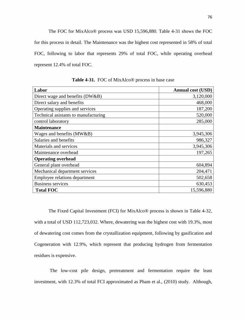
76

The FOC for MixAlco® process was USD 15,596,880. Table 4-31 shows the FOC

for this process in detail. The Maintenance was the highest cost represented in 58% of total

FOC, following to labor that represents 29% of total FOC, while operating overhead

represent 12.4% of total FOC.

Table 4-31. FOC of MixAlco® process in base case

Labor Annual cost (USD)

Direct wage and benefits (DW&B) 3,120,000

Direct salary and benefits 468,000

Operating supplies and services 187,200

Technical asistants to manufacturing 520,000

control laboratory 285,000

Maintenance

Wages and benefits (MW&B) 3,945,306

Salaries and benefits 986,327

Materials and services 3,945,306

Maintenance overhead 197,265

Operating overhead

General plant overhead 604,894

Mechanical department services 204,471

Employee relations department 502,658

Business services 630,453

Total FOC 15,596,880

The Fixed Capital Investment (FCI) for MixAlco® process is shown in Table 4-32,

with a total of USD 112,723,032. Where, dewatering was the highest cost with 19.3%, most

of dewatering cost comes from the crystallization equipment, following by gasification and

Cogeneration with 12.9%, which represent that producing hydrogen from fermentation

residues is expensive.

The low-cost pile design, pretreatment and fermentation require the least

investment, with 12.3% of total FCI approximated as Pham et al., (2010) study. Although,

77

the long residence time of pretreatment and fermentation requires large piles, which have a

volume of 160,000 m3 each (Pham et al., 2010). An installed cost of fermentator is

calculated, scaling to 40 ton/h, based on previous study made by Holtzapple, (2004).

Table 4-32. FCI for MixAlco® process in the base case

% FCI FCI (USD)

Pretreatment & Fermentation 12.7 14,310,330

Dewatering 19.3 21,778,057

Ketonization 6.69 7,543,494

Ketone Hydrogenation 11.7 13,215,510

Gasification & Cogeneration 12.9 14,491,711

Steam Gas Shift & PSA* 7.90 8,913,659

Dehydratation & Oligomerization 9.12 10,276,671

Olefin Hydrogenation 12.2 13,809,600

WWT** - Storage - Utility 7.44 8,384,000

Total FCI 100 112,723,032

The Working Capital Investment (WCI) was calculated as 10% of FCI, with a total

of USD 11,272,303. The Total Capital Investment (TCI) was calculated as WCI plus FCI,

resulting in USD 123,995,335.

Table 4-33 shows the obtained profitability results for MixAlco® process with and

without the time value of money.

Table 4-33. Summary MixAlco® economic results in base case

Parameter Value

Profitability without the time value of money

ROI estimated (%) 14.7

Annual gross (pre tax) profit (USD) 20,786,937

Annual net (after tax) profit (USD) 16,616,185

PBP (years) 4.40

78

Parameter Value

Total operating cost (USD) 52,090,637

FCI (USD) 112,723,032

WCI (USD) 11,272,303

TCI (USD) 123,995,335

Profitability with the time value of money

NPV (USD) 7,296,447

ROI real (%) 11.13

Annual sales (USD) 72,877,573

Tax rate (%) 35

Discount rate (%) 10%

The base case for MixAlco® process results in a ROI of 11.129% that is not the

desirable 15%, but is acceptable in current market conditions. However, the NPV represent

a profitable project in USD 7,296,447. In sensibility analysis the variation of biomass,

gasoline and jet prices showed an improvement in the obtained ROI. Currently, the prices

for those products are: biomass (60.0 USD/gal), gasoline (3.38 USD/gal), and Jet (2.88

USD/gal). Furthermore, the results reported by Pham et al., (2010) shown a ROI

evaluation project of 10.0%.

The PBP is about 4.40 years after start of operation. The cumulative discounted cash

flow for this case is shown in the Figure 4-20. This shown that after paying all the expenses

of the project, the revenues of the project will give net value of MM USD 7.30 in the

present dollars.

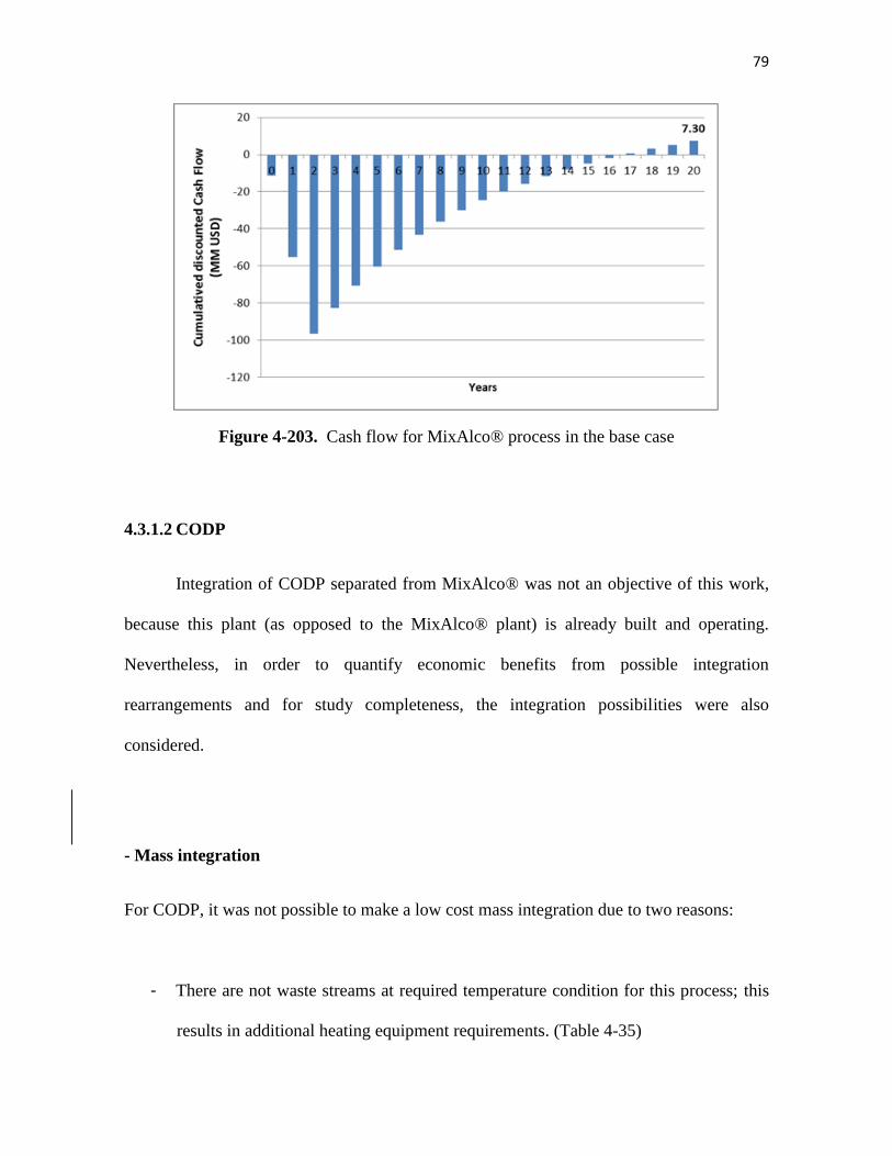
79

Figure 4-203. Cash flow for MixAlco® process in the base case

4.3.1.2 CODP

Integration of CODP separated from MixAlco® was not an objective of this work,

because this plant (as opposed to the MixAlco® plant) is already built and operating.

Nevertheless, in order to quantify economic benefits from possible integration

rearrangements and for study completeness, the integration possibilities were also

considered.

- Mass integration

For CODP, it was not possible to make a low cost mass integration due to two reasons:

- There are not waste streams at required temperature condition for this process; this

results in additional heating equipment requirements. (Table 4-35)

80

- The waste water in CODP (Table 4-35) results in two streams. One of the streams

contains impurities (petroleum fractions) and the other stream is impurity-free

water. The water waste reuse is possible if new separation and heating equipment

are introduced in order to use all the waste water.

Table 4-34 and 4-35 show mass balances obtained for fresh and waste streams in the

simulation.

Table 4-344. Fresh CODP streams

FIRST PRE-

HEATING TRAIN ATMOSPHERIC UNIT

VACUUM

UNIT

CRUDE-IN STEAM-4 STEAM-JT STEAM-5

Temperature(°C) 30.0 353 353 454

Pressure (bar_a) 2.40 5.00 5.00 3.70

Mass Vapor Fraction 0 1.00 1.00 1.00

Mass Liquid Fraction 1.00 0 0 0

Total mass flow (ton/h) 162 3.17 0.600 3.00


Water 0 3.17 0.600 3.00

Ethane 0 0 0 0

Propane 5.48 x10-2 0 0 0

Isobutane 8.23 x10-2 0 0 0

N-Butane 2.21 x10-2 0 0 0

Isopentane 3.71 x10-2 0 0 0

N-Pentane 3.58 x10-2 0 0 0

N-Hexane 4.32 x10-2 0 0 0

Pseudocomponents 160.5 0 0 0

81

Table 4-35. Waste CODP Streams

First pre-heating train Atmospheric Unit Vacuum unit

WAT-SP20 WATSP203 GAST4 WAT-S204

Temperature(°C) 76.1 98.3 97.8 48.9

Pressure (bar_a) 1.70 1.70 1.70 1.20

Mass Vapor Fraction 0 0 1.00 0

Mass Liquid Fraction 1.00 1.00 0 1.00

Total Flow (ton/h) 3.80 1.60 11.3 3.00


Water 3.80 1.60 2.10 3.00

Propane 0 0 0.100 0

Isobutane 0 0 0.100 0

N-Butane 0 0 0.200 0

Isopentane 0 0 0.400 0

N-Pentane 0 0 0.300 0

N-Hexane 0 0 0.400 0

Pseudocomponents 0 0 7.70 0

- Heat integration

Appendix D shows a literature review of heat integration. The base case for CODP

resulted in energetic requirements for heating of 126 GJ/h, and for cooling of 129 GJ/h.

With the current equipment, it was not possible to make low cost energy integration,

because new equipment was required. Furthermore, it was not possible to make power

integration because CODP do not have power generation equipment.

- Cost analysis

Cost analysis for CODP was made in the base case, regardless the inclusion of new

equipment and made integrations (mass, heat) in the process. For this process, it is not

necessary to make a capital investment because it is supposed that CODP plant was already

in operation. However, capital investment was calculated in order to estimate the FCI. This

82

value is necessary to obtain the FOC. Table 4-36 shows the FCI obtained. Where,

atmospheric unit represent the highest cost with 50.9% because all heating and cooling

equipment associated, mainly the furnace and the tower cost.

Table 4-365. FCI for CODP in base case

% FCI TOTAL FCI (USD)

1st-Pre-heating train 11.8 2,165,988

2nd-Pre-heating train 9.30 1,709,220

Atmospheric unit 50.9 9,336,879

Vacuum unit 27.9 5,117,311

Total FCI 100 18,329,399

Table 4-37 shows the VOC for CODP. The total VOC is 838,572,493 USD per

year. This obtained cost is higher than cost obtained for MixAlco® process, because the

crude oil price is 93.6 USD per barrel (643 USD/ton), represented the 99.4% of total VOC.

Although, utilities represent 0.6% of total VOC, this amount 5,097,185 USD/ year.

Table 4-37. VOC of CODP in base case

Rate Prices

Annual cost

(USD)

Feedstock

Crude oil 162 ton/h 643 USD/ton 833,475,308

Utility

Fired Heat 201.3 ton/h 2.50 USD/ton 4,105,591

LP Steam 2.20 ton/h 4.20 USD/ton 74,480


Steam @ 353°C 4.00 ton/h 10.0 USD/ ton 320,000


Electricity 0.28 MW 0.0620 USD/kWh 138,880

Total VOC 838,572,493

The number of total operators was calculated for four process zones. Each of them

was established to need two operators. This resulted in a total of eight operators per shift;

83

and the total shifts are five due to illness, vacations, holidays, training, and overtime during

startups. The labor, maintenance and overhead operating cost accounts were based on

(Seider, Seader, & Lewin, 2004) (Peters, Timmerhaus, & West, 2004). The plant operating

hours were established as 8000 per year. The FOC obtained for CODP was calculated in

USD 5,976,964. Table 4-38 shows the FOC for this process in detail. The labor was the

highest cost represented in 61.3% of total FOC, following to labor that represents 24.7% of

total FOC, while operating overhead represent 14% of total FOC.

Table 4-38. FOC for CODP in base case

Annual cost (USD)

Labor






Maintenance

Wages and benefits (MW&B) 641,529


Materials and services 641,529


Operating overhead





Total FOC 5,976,964

To verify the analysis cost of CODP was supposed as a new plant. The obtained

ROI was 31.2% and the NPV was MM USD 29.

84

4.3.2 Internal modification

The second loop of the proposed methodology covers only internal modifications

adding new units in each plant. With the aim of apply this second step, replacements and

additions of new equipments for MixAlco® process and CODP were made.

4.3.2.1 MixAlco® process

- Mass integration

As explained before (Section 4.3.1.1) mass integration using the resulting impurity-

free water from dewatering and gasification process is the only possibility accounted for in

this work.

- Heat integration

In the MixAlco® process, some streams could not be energetically integrated

because these are needed in the power generation from gasification unit. Also, some

streams are needed in the heat exchanger arrangements in the dewatering process. Table 4-

39 shows the hot and cold streams used for the energy integration.

85

The streams to be cooled were labeled as hot (H), the total streams are 16, meanwhile the streams to be heated were labeled as

cold (C), the total streams are 16. Besides, Table 4-39 shows inlet and outlet temperatures, the mass and heat capacity (MCp), the flow

rate and the enthalpy of the streams. The heating and cooling utility load required for the base case was 4.33x108 kJ/h and 8.21x107

kJ/h, respectively.

Table 4-39. MixAlco® process streams for HEN

Service Inlet T

(°C)

Outlet T

(°C)

MCp

(kJ/°C-h)

Enthalpy

(kJ/h)

Flowrate

(kg/h) Name

H1 130 55 5.61x103 4.21x105 6.30x103 PRET-FER.CACO3REC_To_PRET-FER.CACO3

H2 430 -15 2.93x104 1.31x107 9.59x103 KETONIZA.KET-CACO_To_KETONIZA.KT-CACO3

H3 961 130 5.10x103 4.24x106 3.40x102 KETONIZA.H21_To_KETONIZA.H2-1

H4 500 55 4.21x103 1.87x106 4.06x103 LIME-KIL.CAO_To_LIME-KIL.CAO-CO2

H5 961 130 1.67x103 1.39x106 1.11x102 FINAL.H2-_To_FINAL.H2-1

H6 400 130 2.65x104 7.15x106 7.37x103 FINAL.OLF_To_FINAL.OLEFIN

H7 266 25 1.94x104 4.68x106 5.28x103 FINAL.HC-C4--8_To_FINAL.LIGHT

H8 408 25 7.02x103 2.69x106 2.09x103 FINAL.HC-C9-12_To_FINAL.HEAVY

H9 254 43 2.90x104 6.11x106 2.28x104 GASIFICA.C+H2+H20_To_GASIFICA.H2+

H10 162 94 1.79x105 1.21x107 5.00x103 GASIFICA.STEAMSAT_To_GASIFICA.WATER

H11 268 266 9.83x104 1.97x105 5.28x103 FINAL. CONDENSER T-101

H12 55 46 8.05x105 7.00x106 2.00x105 PRET-FER.SALT3_To_PRET-FER.SALW1



H15 50 41 7.96x105 7.06x106 2.00x105 PRET-FER.H20-FERM_To_PRET-FER.H2O

H16 162 60 5.02x106 5.12x108 2.01x105 DEWATER.WATER_To_DEWATER.WATDISTI

C1 150 165 4.51x106 6.83x107 3.34x104 DEWATER.SALWR1_To_DEWATER.SALWR7

86

Service Inlet T

(°C)

Outlet T

(°C)

MCp

(kJ/°C-h)

Enthalpy

(kJ/h)

Flowrate

(kg/h) Name






C7 163 430 7.86x103 2.10x106 2.52x104 KETONIZA.SAL-DEH_To_KETONIZA.SALT

C8 -15 130 2.25x104 3.26x106 9.59x103 KETONIZA.KT-CACO3_To_KETONIZA.KET

C9 130 300 5.33x104 9.05x106 9.93x103 KETONIZA.ALCOHOL_To_KETONIZA.OH

C10 130 500 9.61x103 3.55x106 9.20x103 LIME-KIL.CACO3-2_To_LIME-KIL.CACO3-3

C11 289 408 4.65x104 5.53x106 2.09x103 FINAL. REBOILER T-101

C16 55 150 5.39x106 5.12x108 2.00x105 DEWATER.SAL-DESC_To_DEWATER.SALT-H20

The hot and the cold curves composite are shown in Figure 4-21, where a hot pinch temperature was 60.5°C, and cold pinch

temperature was 55°C. The grand composite curve is shown in Figure 4-22, where the pinch temperature is shown when the net heat

flow in the process is zero.

87

Figure 4-21. Hot and Cold composite for MixAlco® HEN

Figure 4-22. Grand composite curve for MixAlco® HEN

Heat integration was made using two HEN cases with a ΔTmin of 2°C and 5.5°C; and

one optimized case Minimizing Total Annualized Cost (MTAC) based on the case of ΔTmin

= 5.5°C, for a total of three study cases. Table 4-40 shows the heat integration results of

these cases and the base case.

Pinch point

Pinch point

88

For MixAlco® process, the best heat integration resulted with the optimized case

when a ΔTmin = 5.5°C was used. For heat integration, the hot utilities used were fired heat,

MP steam and LP steam. By the other hand, the cooling utilities used were cooling water

and refrigerant.

The optimum arrangement whit the MTAC, resulted in a heating load of 4.19 x108

kJ/h and a cooling load of 6.85 x107 kJ/h. It results reduced in 8.3% the capital cost and in

8.6% the operating cost compared to the base case.

Table 4-40. Heat integration for MixAlco® process

Base case

HEN proposed

(with integration)

Optimized

MTAC Target

ΔT (2°C) ΔT (5.5°C) ΔT (5.5°C)

Fired Heat (kJ/h) 2.02x107 7.99x106 7.99x106 7.99x106 7.09x106

MP Steam (kJ/h) 4.13x108 4.11x108 4.08x108 4.08x108 4.11x108

Cooling Water (kJ/h) 6.90x107 6.65x107 6.65x107 6.74x107 6.65x107

LP Steam (kJ/h) 0 0 2.70x106 2.70x106 0

Refrigerant (kJ/h) 1.31x107 2.00x106 2.01x106 1.10x106 1.15x106

Heating (kJ/h) 4.33x108 4.19x108 4.19x108 4.19x108 3.83x108

Cooling (kJ/h) 8.21x107 6.85x107 6.85x107 6.85x107 3.29x107

Capital cost (USD) 1.44x107 1.40 x107 1.32 x107 1.34 x107 2.91x107

Operating cost (USD/year) 8.36x106 7.66x106 7.65x106 7.64x106 6.78x106

Figure 4-23 shows the grid diagram that indicates the configuration of the heat

exchangers between the streams in the MixAlco® process. Also, it shows the utilities

streams for heaters and coolers in the best arrangement. Table 4-41 to 4-43 show the

worksheets of each heat exchangers, heaters and coolers including the temperature of each

stream, the area and the heat load.

89

The required heat exchangers are 9, with a total heat load of 5.26x108 kJ/h. The required heaters are 11 for a total heating load

of 4.19x108 kJ/h. And, the required coolers are 15 for a total cooling load of 6.85x107 kJ/h.

Figure 4-23. Grid diagram for MixAlco® HEN

90

Table 4-41. Heat exchangers for MixAlco® HEN

Heat

Exch Cold Stream

Cold T

in (°C)

Cold T

out (°C) Hot Stream

Hot T

in (°C)

Hot T

out (°C)

Load

(kJ/h)

Area

(m2)

E-141 FINAL.REBOILER T-101 289 331

KETONIZA.KET-

CACO_To_KETONIZA.KT-CACO3 362 309 1.55x106 123

E-143 KETONIZA.ALCOHOL_To_KETONIZA.OH 130 300

KETONIZA.KET-


E-116

DEWATER.SAL-

DESC_To_DEWATER.SALT-H20 55 150

DEWATER.WATER_To_DEWATE

R.WATDISTI 162 60 4.99x108 9,326

E-140 FINAL.REBOILER T-101 289 331 FINAL.OLF_To_FINAL.OLEFIN 351 336 3.89x105 23

E-142 KETONIZA.ALCOHOL_To_KETONIZA.OH 130 300 FINAL.OLF_To_FINAL.OLEFIN 336 145 5.06x106 141

E-139 FINAL.REBOILER T-101 331 359 FINAL.OLF_To_FINAL.OLEFIN 400 351 1.30x106 80

E-148

DEWATER.SAL-

DESC_To_DEWATER.SALT-H20 55 55 FINAL.OLF_To_FINAL.OLEFIN 145 130 3.95x105 2

E-115

DEWATER.SAL-


GASIFICA.STEAMSAT_To_GASIFI

CA.WATER 162 94 1.21x107 72

E-117

DEWATER.SALWR3_To_DEWATER.SAL

WR9 150 165

KETONIZA.KET-


Table 4-42. Coolers for MixAlco® HEN

Heat

Exchanger Utility Hot Stream

Hot T in

(°C)

Hot T out

(°C)

Load

(kJ/h)

Area

(m2)

E-132 Cooling Water DEWATER.WATER_To_DEWATER.WATDISTI 162.1 60.0 1.33x107 22.7

E-136 Cooling Water FINAL.HC-C9-12_To_FINAL.HEAVY 407.8 25.0 2.69x106 12.0

E-133 Cooling Water FINAL.HC-C4--8_To_FINAL.LIGHT 266.2 25.0 4.68x106 28.3

E-127 Cooling Water FINAL.H2-_To_FINAL.H2-1 961.0 130.0 1.39x106 2.70

E-125 Cooling Water PRET-FER.SALT4_To_PRET-FER.SALW3 55.0 46.3 7.01x106 33.5

E-147 Cooling Water KETONIZA.KET-CACO_To_KETONIZA.KT-CACO3 173.0 53.1 3.52x106 15.7

91

Heat


Hot T in

(°C)

Hot T out

(°C)

Load

(kJ/h)

Area

(m2)

E-149 Refrigerant 1 KETONIZA.KET-CACO_To_KETONIZA.KT-CACO3 53.1 -15.2 2.01x106 30.3

E-126 Cooling Water PRET-FER.CACO3REC_To_PRET-FER.CACO3 130.0 55.0 4.21x105 9.90

E-130 Cooling Water GASIFICA.C+H2+H20_To_GASIFICA.H2+ 254.0 43.0 6.11x106 798.5

E-128 Cooling Water KETONIZA.H21_To_KETONIZA.H2-1 961.0 130.0 4.24x106 8.30

E-138 Cooling Water FINAL.CONDENSER T-101 268.0 266.0 1.97x105 1.20


E-135 Cooling Water LIME-KIL.CAO_To_LIME-KIL.CAO-CO2 500.0 55.0 1.87x106 138.1


E-129 Cooling Water PRET-FER.H20-FERM_To_PRET-FER.H2O 50.0 41.1 7.06x106 42.0

Table 4-436. Heaters for MixAlco® HEN

Heat

Exchanger Utility Cold Stream

Cold T in

(°C)

Cold T

out (°C)

Load

(kJ/h)

Area

(m2)

E-137 LP Steam KETONIZA.KT-CACO3_To_KETONIZA.KET -15 105 2.70x106 11.0

E-145 Fired Heat KETONIZA.SAL-DEH_To_KETONIZA.SALT 163 430 2.10x106 35.0

E-134 Fired Heat FINAL.REBOILER T-101 359 408 2.29x106 17.0

E-122 MP Steam KETONIZA.KT-CACO3_To_KETONIZA.KET 105 130 5.55x105 2.00

E-124 MP Steam DEWATER.SALWR4_To_DEWATER.SALWR10 150 165 6.83x107 297






E-144 Fired Heat LIME-KIL.CACO3-2_To_LIME-KIL.CACO3-3 130 500 3.55x106 50.0

92

- Cost analysis

The total VOC is shown in Table 4-44 for MixAlco® process with the above

integrations resulted in 35,770,884 USD per year. The VOC saving was achieved in 1.98%

per year, compared to the base case. The mainly difference with the base case is a new

consumption of LP steam, and the reduction of fire heat in 60.5% and refrigerant in 91.6%.

Table 4-44. VOC of MixAlco® process with HEN


Feedstock



Chemical

Lime 0.900 ton/h 70.0 USD/ton 504,000



CaCO3 9.00 ton/h 50.0 USD/ton 3,600,000

Utility





Refrigerant 228.313 m3/h 0.0131 USD/ m3 24,011


Material disposal 6.00 ton/h 18.0 USD/ton 864,000


The FOC obtained for MixAlco® process resulted in 15,498,900 USD per year.

Table 4-45 shows the FOC obtained in detail. The FOC saving was achieved in 0.63% per

year, compared to the base case. The variations were obtained in maintenance and

operating overhead; the labor did not change.

93

The total FCI obtained for this process was USD 111,640,076, in this value the

capital cost saving for HEN integration was discount; reducing the FCI in 0.96% compared

with the base case. The WCI was calculated as 10% of FCI, with a total of USD

11,164,008. The TCI was calculates as the sum of WCI and FCI, resulting in USD

122,804,084.

Table 4-45. FOC of MixAlco® process with HEN

Annual cost (USD)

Labor






Maintenance

Wages and benefits (MW&B) 3,907,403


Materials and services 3,907,403


Operating overhead





15,498,900

Table 4-46 shows the obtained profitability results for MixAlco® process with and

without the time value of money.

94

Table 4-46. Summary MixAlco® economic results with HEN

Parameter Value


ROI estimated (%) 15.65

Annual gross (pre tax) profit (USD) 21,607,790

Annual net (after tax) profit (USD) 17,477,107

PBP (years) 4.23

Total operating cost (USD) 51,269,784

FCI (USD) 111,640,076

WCI (USD) 11,164,008

TCI (USD) 122,804,084


NPV (USD) 11,722,637

ROI real (%) 11.809

Annual sales (USD) 72,877,573

Tax rate (%) 35.0

Discount rate (%) 10.0

The MixAlco® process integration results in a ROI of 11.8% acceptable in current

market conditions, a ROI increment of 0.68% was obtained compared with the base case.

The NPV represent a profitable project in USD 11,722,637, with a NPV increment of

37.8% compared with the base case.




present dollars.

95

Figure 4-24. Cash flow for MixAlco® process with HEN

4.3.2.2 CODP

- Mass integration

According to section 4.3.1.2, there is not possible to make a mass integration for CODP.

- Heat integration

Table 4-47 shows the hot and cold streams of the process available to make the heat

integration. The streams to be cooled were labeled as hot (H), the total streams are 15,

meanwhile the streams to be heated were labeled as cold (C), the total streams are 7. Also,

it shows the inlet and outlet temperatures, the mass and heat capacity (MCp), the flow rate

and the enthalpy of the streams in CODP.

96

Table 4-47. Process streams for CODP

Service Inlet T

(°C)

Outlet T

(°C)

MCp

(kJ/°C-h)

Enthalpy

(kJ/h)

Flowrate

(kg/h) Name

H1 144 44 4.17x105 4.19x107 6.48x104 1-TRAIN.OVHT204_To_1-TRAIN.OVH202

H2 236 138 2.16x105 2.13x107 8.80x104 1-TRAIN.DIE203_To_1-TRAIN.DIEST204

H3 324 75 8.91x104 2.22x107 3.69x104 2-TRAIN.HVGO_To_2-TRAIN.GPVT205

H4 390 285 1.29x105 1.35x107 4.66x104 2-TRAIN.ASFP205_To_2-TRAIN.ASPHALT

H5 289 236 2.37x105 1.25x107 8.80x104 2-TRAIN.DIEST204_To_2-TRAIN.DISE205

H6 277 227 4.28x105 2.15x107 1.62x105 ATM-UNIT.SP-202_heat

H7 193 68 4.64x104 5.81x106 1.99x104 ATM-UNIT.JETT204_To_ATM-UNIT.JET-T204

H8 284 148 1.35x105 1.84x107 5.29x104 [email protected][email protected]

H9 304 288 1.29x105 2.03x106 4.62x104

[email protected]_To_MPACAL_Return@ATM-

UNIT.T-204

H10 144 98 4.45x105 2.08x107 6.48x104 To [email protected]_TO_ATM-UNIT.NAPHT204

H11 213 34 1.14x104 2.04x106 5.26x103 VAC-UNIT.LVGOT205_To_VAC-UNIT.LVGO-205

H12 60 49 6.52x105 7.24x106 3.00x103 VAC-UNIT.SP-204_heat



H15 324 233 8.69x103 7.87x105 3.24x103

[email protected]_To_MPACAL_Return@VAC-

UNIT.T-205

C1 31 181 3.46x105 5.22x107 1.62x105 1-TRAIN.CRUDE-IN_To_1-TRAIN.CRDTP1

C2 44 76 1.51x105 4.87x106 6.48x104 1-TRAIN.SP-201_heat

C3 183 277 4.16x105 3.90x107 1.62x105 2-TRAIN.CRDTP1R_To_2-TRAIN.CRDE207

C4 228 381 5.14x105 7.87x107 1.62x105 ATM.UNIT.FURNACE

C5 148 279 1.35x105 1.77x107 5.29x104 ATM-UNIT.MPAT204_To_ATM-UNIT.MPAM201

C6 98 98 7.21x104 3.44x104 4.40x103 ATM-UNIT.SP-203_heat

C7 366 432 3.66x105 2.44x107 8.88x104 VAC-UNIT.CRDT204_To_VAC-UNIT.CREDT205

97

The hot and the cold curves composite are shown in Figure 4-25, where a hot pinch

temperature was 277.2°C, and cold pinch temperature was 271.8°C. The grand composite

curve is shown in Figure 4-26 where the pinch temperature is shown when the net heat flow

in the process is zero.

Figure 4-25. Hot and Cold composite for CODP HEN

Figure 4-26. Grand composite curve for CODP HEN

The heat integration was made using two HEN cases with a ΔTmin of 4°C and

5.35°C, and two optimized cases based on the case of ΔTmin = 5.35°C one to optimized the

Pinch point

Pinch point

98

MTAC and the other, to optimize de minimum heat area, for a total of four cases. Table 4-

48 shows the heat integration results of these cases and the base case.

For CODP, the best heat integration resulted when optimized the MTAC and

ΔTmin= 5.3°C was used. In CODP heat integration, the hot utilities used were fired heat and

LP steam. By the other hand, the cooling utility used was cooling water.

The heating and cooling utility load required for the base case was 1.26 x108kJ/h and

1.29x108kJ/h, respectively. The optimum arrangement whit the MTAC resulted in a heating

load of 7.45 x107 kJ/h and a cooling load of 7.65 x107 kJ/h. It results reduced in 39% the

operating cost, but increased in 78% the capital cost compared with the base case.

Table 4-48. Summary of HEN cases for CODP

Base case HEN proposed

(with integration) Optimized

MTAC

Optimized

Min Area Target

ΔT

(5.35°C)

ΔT

(4°C)

ΔT

(5.35°C)

ΔT

(5.35°C)

Fired Heat (kJ/h) 1.21x108 7.33x107 7.36x107 7.45x107 7.33x107

Cooling Water (kJ/h) 1.29x108 7.53x107 7.56x107 7.65x107 7.53x107

LP Steam (kJ/h) 4.90x106 3.44x104 3.44x104 3.44x104 3.44x104

Heating (kJ/h) 1.26x108 7.34x107 7.37x107 7.45x107 7.34x107 5.85x107

Cooling (kJ/h) 1.29x108 7.53x107 7.56x107 7.65x107 7.53x107 6.04x107

Capital cost (USD) 8.50x106 1.81x107 1.93x107 1.51x107 1.67x107 4.61x107

Operating cost (USD/year) 4.40x106 2.62x106 2.63x106 2.66x106 2.62x106 1.91x106


exchangers between the streams in the CODP. Also, it shows the utilities streams

arrangements.

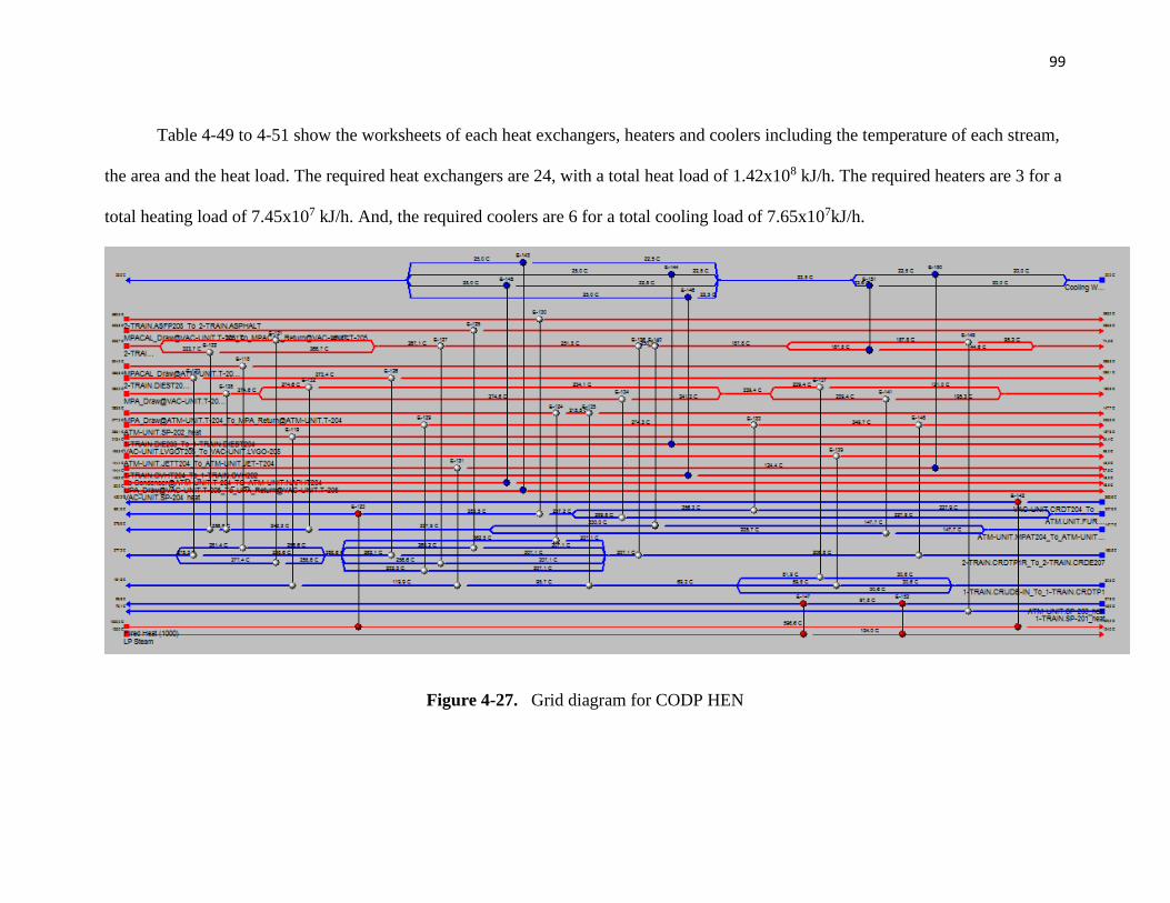
99

Table 4-49 to 4-51 show the worksheets of each heat exchangers, heaters and coolers including the temperature of each stream,

the area and the heat load. The required heat exchangers are 24, with a total heat load of 1.42x108 kJ/h. The required heaters are 3 for a

total heating load of 7.45x107 kJ/h. And, the required coolers are 6 for a total cooling load of 7.65x107kJ/h.

Figure 4-27. Grid diagram for CODP HEN

100

Table 4-49. Heat exchangers in the best CODP case

Heat

Exch Cold Stream

Cold

T in

(°C)

Cold T


Hot T

in

(°C)

Hot T

out (°C)

Load

(kJ/h)

Area

(m2)

E-148 2-TRAIN.CRDTP1R_To_2-

TRAIN.CRDE207 183 207 ATM-UNIT.SP-202_heat 250 227 9.73x106 405

E-133 ATM.UNIT.FURNACE 228 256 ATM-UNIT.SP-202_heat 274 250 1.06x107 1605

E-135 1-TRAIN.CRUDE-IN_To_1-

TRAIN.CRDTP1 69 96

[email protected]

[email protected] 216 148 9.19x106 103

E-149 1-TRAIN.SP-201_heat 44 76 2-TRAIN.HVGO_To_2-TRAIN.GPVT205 188 95 4.87x106 132


TRAIN.CRDE207 207 262 2-TRAIN.DIEST204_To_2-TRAIN.DISE205 273 236 8.86x106 320

E-128 ATM-UNIT.MPAT204_To_ATM-

UNIT.MPAM201 242 257

[email protected]


E-134 ATM.UNIT.FURNACE 228 259 [email protected]



TRAIN.CRDE207 207 207 2-TRAIN.HVGO_To_2-TRAIN.GPVT205 252 251 9.64x104 2


TRAIN.CRDE207 259 281

[email protected]

[email protected]

204

304 288 2.03x106 52


UNIT.MPAM201 148 230 2-TRAIN.HVGO_To_2-TRAIN.GPVT205 251 188 5.61x106 184


TRAIN.CRDTP1 31 82

[email protected]



TRAIN.CRDTP1 31 60

ATM-UNIT.JETT204_To_ATM-UNIT.JET-

T204 193 68 5.81x106 92






TRAIN.CRDTP1 96 120 1-TRAIN.OVHT204_To_1-TRAIN.OVH202 144 124 8.37x106 386



[email protected]

[email protected] 233 7.87x105 15

101

Heat

Exch Cold Stream

Cold

T in

(°C)

Cold T


Hot T

in

(°C)

Hot T

out (°C)

Load

(kJ/h)

Area

(m2)

205




TRAIN.CRDTP1 120 181 1-TRAIN.DIE203_To_1-TRAIN.DIEST204 236 138 2.13x107 773



[email protected]


E-130 ATM.UNIT.FURNACE 257 283 2-TRAIN.ASFP205_To_2-TRAIN.ASPHALT 390 285 1.35x107 534



[email protected]




[email protected]






Table 4-50. Coolers in the best CODP case

Heat


Hot T

in (°C)

Hot T

out (°C)

Load

(kJ/h)

Area

(m2)

E-150 Cooling Water 1-TRAIN.OVHT204_To_1-TRAIN.OVH202 124 44 3.36x107 229

E-144 Cooling Water VAC-UNIT.LVGOT205_To_VAC-UNIT.LVGO-205 213 34 2.04x106 18

E-146 Cooling Water To [email protected]_TO_ATM-UNIT.NAPHT204 144 98 2.08x107 95

E-151 Cooling Water 2-TRAIN.HVGO_To_2-TRAIN.GPVT205 188 45 5.22x106 43

E-145 Cooling Water

[email protected][email protected]

205 143 49 7.62x106

55

E-143 Cooling Water VAC-UNIT.SP-204_heat 60 49 7.24x106 349

102

Table 4-51. Heaters in the best CODP case

Heat

Exchanger Utility Cold Stream

Cold T

in (°C)

Cold T

out (°C)

Load

(kJ/h)

Area

(m2)

E-123 Fired Heat ATM.UNIT.FURNACE 283 381 5.01x107 450

E-147 LP Steam ATM-UNIT.SP-203_heat 98.0 98.0 3.44x104 2.00

E-142 Fired Heat VAC-UNIT.CRDT204_To_VAC-

UNIT.CREDT205 366 432 2.44x107 1,001

- Cost analysis

The total VOC for CODP was shown in Table 4-52 with the above integrations resulted

in USD 836,837,003 per year. The VOC saving was achieved in 1,735,491 USD per year.

The FOC for CODP did not change for the base case, because the operator’s number and

salaries kept equal. Although VOC saving was achieved, a capital cost must be assumed for

installation of new heaters, coolers and heat exchangers.

Table 4-527. VOC of CODP with HEN


Feedstock


Utility

Fired Heat 124.2 ton/h 2.50 USD/ton 2,532,560

LP Steam 0.0160 ton/h 4.20 USD/ton 523





Total VOC 836,837,003

This new capital cost was USD 15,010,866. CODP integration results in a ROI of

41.8% and a NPV of MM USD 39.165. To compare the convenience of heat integration

103

into CODP, the profitability of CODP integrated as a new plant was evaluated, as in the

base case. The results show that CODP integration had a reduction of ROI in 3.5%, but a

NPV increment in MM USD 2.7 was obtained compared to the base case.

4.3.3 External modification

The third loop of the proposed methodology covers only external modifications

adding new production lines for linkage (retrofitting analysis) between MixAlco® process

and CODP (Figure 4-28). With the aim of applying this third step, additions of new

production lines for the linkage were made. Due to assumption that CODP plant was

already in operation, MixAlco® was added as a new production line in the CODP.

- Mass integration

The mass integration was performed as suggested in Section 4.3.1.1, that is, using the

resulting impurity-free water from the dewatering and gasification inside MixAlco®

process. Additionally, no other opportunity for integration was identified because calcium

carbonate (the other fresh stream required in MixAlco® process) is not involved in any of

the operations of CODP.

However, considered the water demand in feed handling process (for quick lime

hydration); and water lost in pretreatment and fermentation process.

104

Figure 4-28. MixAlco® and CODP simulation integrated

It was possible to make a mass integration between both processes through the water (waste impurity-free water from CODP

and needed water in feed handling, fermentation and pretreatment). The material water disposal in the MixAlco® process was around

6 ton/h, with a treatment cost of 18USD/ton. This resulted in a total operating cost of 864,000 USD per year. Through the mass

integration made, the material disposal cost was saved. Additionally, a FCI saving was achieved in USD 148,598 for the purchased

equipment and installation of this process.

105

On the other hand, integration of the biomass feedstock into the CODP was not useful

because units required for treating the biomass are not available in the CODP.

- Heat integration

It was possible to establish two heat integration cases. The first case was related to

integration of the remaining streams for both processes after heat integration within each

plant. The second case was related to integration between the remaining streams of CODP

after heat integration within the plant, and the base case of MixAlco® process.

4.3.3.1 Case 1.

The first case was integration between MixAlco® process and CODP after heat

integration within each plant, and evaluating the retrofitting analysis of the linkage.

- Heat integration

The heat integration in this case is joining the results in numerals 4.3.2.1 for

MixAlco® process with the results in numeral 4.3.2.2 for CODP.

The heating and cooling utility load required for the both plants was 5.59x108 kJ/h

and 2.11x108 kJ/h, respectively. The optimum arrangement whit the MTAC, resulted in a

heating load of 4.94 x108 kJ/h and a cooling load of 1.45 x108 kJ/h. It results reduced in

24.1% the operating cost and increased in 19.1% the capital cost compared with the base

case (Table 4-53). For the retrofitting analysis 33 heat exchangers are needed, 14 heaters

and 21 coolers.

106

Table 4-53. Heat integration for MixAlco® and CODP in case 1

Case 1

Base case

joining both

plants

MixAlco®

with internal

HEN

CODP with

internal

HEN

MixAlco®

and CODP

case 1

Fired Heat (kJ/h) 1.41x108 7.99x106 7.45x107 8.25x107

MP Steam (kJ/h) 4.13x108 4.08x108 0 4.08x108

Cooling Water (kJ/h) 1.98x108 6.74x107 7.65x107 1.44x108

LP Steam (kJ/h) 4.90x106 2.70x106 3.44x104 2.73x106

Refrigerant (kJ/h) 1.31x107 1.10x106 0 1.10x106

Heating (kJ/h) 5.59x108 4.19x108 7.45x107 4.94x108

Cooling (kJ/h) 2.11x108 6.85x107 7.65x107 1.45x108

Capital cost (USD) 2.29x107 1.32x107 1.51x107 2.83x107

Operating cost (USD/year) 1.28x107 7.63x106 2.65x106 1.03x107

- Cost analysis

Table 4-54. VOC of MixAlco® process in case 1


Feedstock



Chemical

Lime 0.900 ton/h 70.0 USD/ton 504,000



CaCO3 9.00 ton/h 50.0 USD/ton 3,600,000

Utility


MP Steam 206 ton/h 4.40 USD/ton 7,184,465

Cooling Water 3,224 m3/h 0.00400 USD/m3 114,407


Refrigerant 228 m3/h 0.0131 USD/ m3 24,011



107

The total VOC for MixAlco® process with the above integrations resulted in

34,906,884 USD per year, with a reduction of 4.55%, compare with the base case. Table 4-

54 shows the VOC in detail. The total VOC for CODP is the same obtained in numeral

5.3.2.2 (836,837,003 USD per year), with a reduction in 0.21%, compare with the base

case.

The FOC obtained for MixAlco® process resulted in 15,485,455 USD per year; with a

reduction of 0.72%, compare with the base case. The FOC for CODP did not change for the

base case, because the operator’s number and salaries kept equal. Table 4-55 shows a

compiled FOC obtained for MixAlco® and CODP.

Table 4-558. FOC of MixAlco® and CODP in case 1

Annual cost (USD)

MixAlco® CODP

Labor

Direct wage and benefits (DW&B) 3,120,000 2,496,000

Direct salary and benefits 468,000 374,400

Operating supplies and services 187,200 149,760

Technical asistants to manufacturing 520,000 416,000

control laboratory 285,000 228,000

Maintenance

Wages and benefits (MW&B) 3,902,202 641,529

Salaries and benefits 975,550 160,382

Materials and services 3,902,202 641,529

Maintenance overhead 195,110 32,076

Operating overhead

General plant overhead 601,068 260,734

Mechanical department services 203,178 88,135

Employee relations department 499,479 216,666

Business services 626,466 271,751

Total FOC 15,485,455 5,976,964

108

The total FCI obtained for MixAlco® process is USD 111,491,478; in this value

capital costs savings for mass and heat integration were discount; resulting in a reduction of

1.10% compared with the base case. The WCI was USD 11,149,148, and the TCI results in

USD 122,640,626.

The total FCI for CODP is USD 15,010,866, because an investment is required for

the new heat equipment arrangement. In CODP possible revenue from selling heat

equipment to be replaced, was no accounted.

Table 4-56 shows the obtained profitability results for MixAlco® process and CODP, with

and without the time value of money applying the integration mentioned in this numeral.

Table 4-56. Summary MixAlco® economic results in case 1

MixAlco® with integration CODP with integration

Parameter Value Value


ROI estimated (%) 16.47 72.49

Annual gross (pre tax) profit (USD) 22,485,234 11,437,226

Annual net (after tax) profit (USD) 18,360,049 10,881,824

PBP (years) 3.55 1.19

Total operating cost (USD) 50,392,339 842,813,966

FCI (USD) 111,491,478 15,010,866

WCI (USD) 11,149,148 1,501,087

TCI (USD) 122,640,626 16,511,953


NPV (USD) 15,699,518 39,165,307

ROI real (%) 12.4 41.8

Annual sales (USD) 72,877,573 854,251,193

Tax rate (%) 35 35

Discount rate (%) 10 10

109

The retrofitting analysis in case 1 for MixAlco® process results in a ROI of 12.4%

acceptable in current market conditions; a ROI increment in 1.3% compared with the base

case. The NPV represent a profitable project in MM USD 15.7, with a NPV increment of





present dollars.

For this study case, CODP results in a ROI of 41.8% and a NPV of MM USD

39.17; as shown in numeral 5.3.2.2 a ROI reduction of 3.5% was obtained, but a NPV

increment of MM USD 2.7 compared to the base case. The PBP is about 1.19 years

assuming as a new plant.

Figure 4-29. Cash flow of MixAlco® process in case 1

110

4.3.3.2 Case 2.

The second case is related to integration between the remaining streams of CODP after heat integration within the plant, and the

base case of MixAlco® process. Although there was an increased in the capital cost for CODP after its heat integration, there was also

a reduction in operation costs around 39%. This was the main reason to make the retrofitting analysis between MixAlco® and CODP

after heat integration within the CODP plant.

Table 4-57. Process streams for case 2

Service Inlet T

(°C)

Outlet T

(°C)

MCp

(kJ/°C-h)

Enthalpy

(kJ/h)

Flowrate

(kg/h) Name

H1 130 55 5.61x103 4.21x105 6.30x103 PRET-FER.CACO3REC_To_PRET-FER.CACO3

H2 430 -15 2.93x104 1.31x107 9.59x103 KETONIZA.KET-CACO_To_KETONIZA.KT-CACO3

H3 961 130 5.10x103 4.24x106 3.40x102 KETONIZA.H21_To_KETONIZA.H2-1

H4 500 55 4.22x103 1.88x106 4.06x103 LIME-KIL.CAO_To_LIME-KIL.CAO-CO2

H5 961 130 1.67x103 1.39x106 1.11x102 FINAL.H2-_To_FINAL.H2-1

H6 400 130 2.65x104 7.15x106 7.37x103 FINAL.OLF_To_FINAL.OLEFIN

H7 266 25 1.94x104 4.68x106 5.28x103 FINAL.HC-C4--8_To_FINAL.LIGHT

H8 408 25 7.02x103 2.69x106 2.09x103 FINAL.HC-C9-12_To_FINAL.HEAVY

H9 254 43 2.89x104 6.09x106 2.28x104 GASIFICA.C+H2+H20_To_GASIFICA.H2+

H10 165 93 1.69x105 1.22x107 5.00x103 GASIFICA.STEAMSAT_To_GASIFICA.WATER

H11 268 266 9.83x104 1.97x105 5.28x103 FINAL. CONDENSER T-101




111

Service Inlet T

(°C)

Outlet T

(°C)

MCp

(kJ/°C-h)

Enthalpy

(kJ/h)

Flowrate

(kg/h) Name

H15 50 42 8.35x105 7.06x106 2.00x105 PRET-FER.H20-FERM_To_PRET-FER.H2O

H16 163 60 4.88x106 5.03x108 2.01x105 DEWATER.WATER_To_DEWATER.WATDISTI

H17 124 44 4.17x105 4.19x107 6.48x104 1-TRAIN.OVHT204_To_1-TRAIN.OVH202

H18 188 75 8.91x104 2.24x107 3.69x104 2-TRAIN.HVGO_To_2-TRAIN.GPVT205

H19 144 98 4.64x105 2.16x107 6.48x104 To [email protected]_TO_ATM-UNIT.NAPHT204

H20 212 34 1.14x104 2.02x106 5.26x103 VAC-UNIT.LVGOT205_To_VAC-UNIT.LVGO-205

H21 60 49 6.52x105 7.24x106 3.00x103 VAC-UNIT.SP-204_heat








C7 163 430 7.86x103 2.10x106 2.52x104 KETONIZA.SAL-DEH_To_KETONIZA.SALT

C8 -15 130 2.25x104 3.26x106 9.59x103 KETONIZA.KT-CACO3_To_KETONIZA.KET

C9 130 300 5.32x104 9.05x106 9.93x103 KETONIZA.ALCOHOL_To_KETONIZA.OH

C10 130 500 9.61x103 3.55x106 9.20x103 LIME-KIL.CACO3-2_To_LIME-KIL.CACO3-3

C11 289 408 4.65x104 5.53x106 2.09x103 FINAL. REBOILER T-101

C12 55.0 149.9 5.39x106 5.12x108 2.00x105 DEWATER.SAL-DESC_To_DEWATER.SALT-H20

C13 284 381 5.14x105 7.87x107 1.62x105 ATM.UNIT.FURNACE

C14 97.8 98.3 7.20x104 3.44x104 4.40x103 ATM-UNIT.SP-203_heat

C15 366 432 3.73x105 2.48x107 8.88x104 VAC-UNIT.CRDT204_To_VAC-UNIT.CREDT205

112

- Heat integration

Table 4-57 shows the hot and cold streams of the process available to make the heat

integration. Also, it shows the inlet and outlet temperatures, the mass and heat capacity

(MCp), the flow rate and the enthalpy of the streams in CODP. The streams to be cooled

were 22; meanwhile the streams to be heated were 15.

The hot and the cold curves composite are shown in Figure 4-30, where a hot pinch

temperature was 155.4°C, and cold pinch temperature was 150°C. The grand composite

curve is shown in Figure 4-31; where the pinch temperature is shown when the net heat

flow in the process is zero.

Figure 4-30. Hot and Cold composite for case 2

Pinch point

113

Figure 4-31. Grand composite curve for case 2

For MixAlco® and CODP, the best heat integration resulted when a ΔTmin = 5.5°C

was used. In the heat integration, the hot utilities used were fired heat, MP steam and LP

steam. By the other hand, the cooling utilities used were cooling water and refrigerant.

The heating and cooling utility load required for the base case was 5.59x108 kJ/h and

2.11x108 kJ/h, respectively. The best heat integration resulted in a heating load of

5.2x108kJ/h and a cooling load of 1.55 x108 kJ/h. It results reduced in 11.21% the operating

cost, but increased in 40.25% the capital cost compared with the base case. Table 4-58

summarizes these results.

Pinch

point

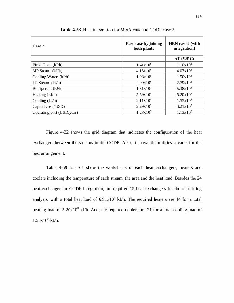
114

Table 4-58. Heat integration for MixAlco® and CODP case 2

Case 2 Base case by joining

both plants

HEN case 2 (with

integration)

ΔT (5.5°C)

Fired Heat (kJ/h) 1.41x108 1.10x108

MP Steam (kJ/h) 4.13x108 4.07x108

Cooling Water (kJ/h) 1.98x108 1.50x108

LP Steam (kJ/h) 4.90x106 2.79x106

Refrigerant (kJ/h) 1.31x107 5.38x106

Heating (kJ/h) 5.59x108 5.20x108

Cooling (kJ/h) 2.11x108 1.55x108

Capital cost (USD) 2.29x107 3.21x107

Operating cost (USD/year) 1.28x107 1.13x107


exchangers between the streams in the CODP. Also, it shows the utilities streams for the

best arrangement.

Table 4-59 to 4-61 show the worksheets of each heat exchangers, heaters and

coolers including the temperature of each stream, the area and the heat load. Besides the 24

heat exchanger for CODP integration, are required 15 heat exchangers for the retrofitting

analysis, with a total heat load of 6.91x108 kJ/h. The required heaters are 14 for a total

heating load of 5.20x108 kJ/h. And, the required coolers are 21 for a total cooling load of

1.55x108 kJ/h.

115

Figure 4-32. Grid diagram for case 2

Table 4-59. Heat exchangers for case 2

Heat

Exch Cold Stream

Cold T

in (°C)

Cold T


Hot T

in (°C)

Hot T

out (°C)

Load

(kJ/h)

Area

(m2)

E-119

DEWATER.SAL-


GASIFICA.STEAMSAT_To_GASIFICA.W

ATER 162 94 1.21x107 76

E-166

DEWATER.SAL-

DESC_To_DEWATER.SALT-H20 55 55 FINAL.OLF_To_FINAL.OLEFIN 165 130 9.33x105 3

E-153

KETONIZA.ALCOHOL_To_KETONI

ZA.OH 150 286

KETONIZA.KET-


116

Heat

Exch Cold Stream

Cold T

in (°C)

Cold T


Hot T

in (°C)

Hot T

out (°C)

Load

(kJ/h)

Area

(m2)

E-120

DEWATER.SAL-


DEWATER.WATER_To_DEWATER.WAT

DISTI 162 72 4.51x108 5,875

E-122


ZA.OH 286 300 FINAL.OLF_To_FINAL.OLEFIN 400 372 7.34x105 4

E-155


ZA.OH 130 150 2-TRAIN.HVGO_To_2-TRAIN.GPVT205 160 173 1.07x106 54

E-157

DEWATER.SAL-

DESC_To_DEWATER.SALT-H20 51 55 2-TRAIN.HVGO_To_2-TRAIN.GPVT205 173 75 1.93x107 199

E-152


ZA.OH 150 286 FINAL.OLF_To_FINAL.OLEFIN 304 165 3.66x106 149

E-121

DEWATER.SALWR2_To_DEWATER

.SALWR8 150 165

KETONIZA.KET-


E-123

DEWATER.SALWR2_To_DEWATER

.SALWR8 150 165 GASIFICA.C+H2+H20_To_GASIFICA.H2+ 254 201 1.55x106 262

E-141

DEWATER.SAL-

DESC_To_DEWATER.SALT-H20 55 62 1-TRAIN.OVHT204_To_1-TRAIN.OVH202 121 103 1.59x107 153

E-143 ATM.UNIT.FURNACE 249 254 FINAL.OLF_To_FINAL.OLEFIN 372 304 1.82x106 37

E-124

DEWATER.SAL-

DESC_To_DEWATER.SALT-H20 62 148 2-TRAIN.HVGO_To_2-TRAIN.GPVT205 188 160 1.19x107 149

E-144 ATM.UNIT.FURNACE 284 289

KETONIZA.KET-


E-142

DEWATER.SAL-


To [email protected]

204_TO_ATM-UNIT.NAPHT204 144 98 2.08x107 147

E-148 2-TRAIN.CRDTP1R_ToCRDE207 183 207 ATM-UNIT.SP-202_heat 250 227 9.73x106 405

E-133 ATM.UNIT.FURNACE 228 256 ATM-UNIT.SP-202_heat 274 250 1.06x107 1,605

E-135

1-TRAIN.CRUDE-IN_To_1-

TRAIN.CRDTP1 69 96

[email protected]


E-149 1-TRAIN.SP-201_heat 44 76 2-TRAIN.HVGO_To_2-TRAIN.GPVT205 188 95 4.87x106 132

E-126

2-TRAIN.CRDTP1R_To_2-


E-128

ATM-UNIT.MPAT204_To_ATM-


[email protected]


E-134 ATM.UNIT.FURNACE 228 259 [email protected] 275 241 4.49x106 600

117

Heat

Exch Cold Stream

Cold T

in (°C)

Cold T


Hot T

in (°C)

Hot T

out (°C)

Load

(kJ/h)

Area

(m2)

[email protected]

E-136


TRAIN.CRDE207 206,8 207,1 2-TRAIN.HVGO_To_2-TRAIN.GPVT205 251,8 250,7 9.64x104 2

E-118



[email protected]

[email protected]

204 304 288 2.03x106 52

E-140



E-137


TRAIN.CRDTP1 31 82

[email protected]


E-139


TRAIN.CRDTP1 31 60

ATM-UNIT.JETT204_To_ATM-UNIT.JET-

T204 193 68 5.81x106 92

E-129



E-127



E-131 1-TRAIN.CRUDE-IN_.CRDTP1 96 120 1-TRAIN.OVHT204_To_1-TRAIN.OVH202 144 124 8.37x106 386

E-125



[email protected]

[email protected]

205 324 233 7.87x105 15

E-121 2-TRAIN.CRDTP1R_To.CRDE207 259 277 2-TRAIN.HVGO_To_2-TRAIN.GPVT205 324 268 2.03x106 84

E-119


TRAIN.CRDTP1 120 181 1-TRAIN.DIE203_To_1-TRAIN.DIEST204 236 138 2.13x107 773

E-141



[email protected]


E-130 ATM.UNIT.FURNACE 257 283

2-TRAIN.ASFP205_To_2-

TRAIN.ASPHALT 390 285 1.35x107 534

E-132



[email protected]


E-124



[email protected]


E-120 2-TRAIN.CRDTP1R_To_CRDE207 259 275 2-TRAIN.DIEST204_To_2-TRAIN.DISE205 289 273 3.66x106 163

E-122 ATM-UNIT.MPAT204_To.MPAM201 257 279 2-TRAIN.HVGO_To_2-TRAIN.GPVT205 324 267 3.02x106 122

118

Table 4-60. Coolers for case 2

Heat


Hot T in

(°C)

Hot T

out (°C)

Load

(kJ/h)

Area

(m2)

E-134 Cooling Water PRET-FER.SALT3_To_PRET-FER.SALW1 55 46 7.00x106 35

E-136 Cooling Water FINAL.H2-_To_FINAL.H2-1 961 130 1.39x106 3

E-168 Cooling Water FINAL.HC-C4--8_To_FINAL.LIGHT 266 25 4.68x106 26

E-162 Cooling Water FINAL.HC-C9-12_To_FINAL.HEAVY 408 25 2.69x106 12


E-147 Cooling Water FINAL.CONDENSER T-101 268 266 1.97x105 1

E-149 Cooling Water VAC-UNIT.LVGOT205_To_VAC-UNIT.LVGO-205 213 34 2.04x106 17

E-133 Cooling Water VAC-UNIT.SP-204_heat 60 49 7.24x106 354

E-169 Refrigerant KETONIZA.KET-CACO_To_KETONIZA.KT-CACO3 9 -15 7.00x105 18


E-148 Cooling Water PRET-FER.CACO3REC_To_PRET-FER.CACO3 130 55 4.21x105 10

E-150 Cooling Water GASIFICA.C+H2+H20_To_GASIFICA.H2+ 201 43 4.57x106 713

E-138 Cooling Water PRET-FER.H20-FERM_To_PRET-FER.H2O 50 41 7.06x106 44

E-140 Cooling Water

[email protected]_To_UPA_Return@VAC-

UNIT.T-205 143 49 7.62x106

55

E-164 Refrigerant KETONIZA.KET-CACO_To_KETONIZA.KT-CACO3 168 9 3.53x106 19



E-137 Cooling Water KETONIZA.H21_To_KETONIZA.H2-1 961 130 4.24x106 8

E-163 Cooling Water DEWATER.WATER_To_DEWATER.WATDISTI 72 60 6.14x107 181

E-165 Refrigerant KETONIZA.KET-CACO_To_KETONIZA.KT-CACO3 168 9 1.14x106 6

E-146 Cooling Water LIME-KIL.CAO_To_LIME-KIL.CAO-CO2 500 55 1.87x106 141

119

Table 4-61. Heaters for case 2

Heat Exchanger Utility Cold Stream Cold T in

(°C)

Cold T out

(°C)

Load

(kJ/h)

Area

(m2)


E-156 MP Steam ATM-UNIT.SP-203_heat 98 98 3.44x104 1

E-160 Fired Heat VAC-UNIT.CRDT204_To_VAC-UNIT.CREDT205 366 432 2.44x107 1013



E-159 Fired Heat LIME-KIL.CACO3-2_To_LIME-KIL.CACO3-3 130 500 3.55x106 94

E-161 Fired Heat KETONIZA.SAL-DEH_To_KETONIZA.SALT 163 430 2.10x106 44


E-130 MP Steam KETONIZA.KT-CACO3_To_KETONIZA.KET 109 130 4.63x105 2

E-125 Fired Heat ATM.UNIT.FURNACE 264 381 7.47x107 659

E-158 Fired Heat FINAL.REBOILER T-101 289 408 5.53x106 191

E-151 LP Steam KETONIZA.KT-CACO3_To_KETONIZA.KET -15 109 2.79x106 12



- Cost analysis

The total VOC for MixAlco® process with the above integrations resulted in 35,160,509 USD per year, with a reduction of

3.79%, compare with the base case. Table 4-62 shows the VOC for MixAlco® process in detail. The total VOC for CODP resulted in

837,612,499 USD per year, with a reduction of 0.11%, compare with the base case. Table 4-63 shows the VOC for CODP in detail.

120

Table 4-62. VOC of MixAlco® process in case 2


Feedstock



Chemical

Lime 0.900 ton/h 70.0 USD/ton 504,000



CaCO3 9.00 ton/h 50.0 USD/ton 3,600,000

Utility





Refrigerant 1,120 m3/h 0.0131 USD/ m3 117,791



Table 4-63. VOC of CODP in case 2


Feedstock


Utility

Fired Heat 165 ton/h 2.50 USD/ton 3,369,029

LP Steam 0.0160 ton/h 4.20 USD/ton 546

Cooling Water 1,937 m3/h 0.00400 USD/m3 68,735




Total VOC 837,612,499

The FOC obtained for MixAlco® process resulted in 15,429,731 USD per year;

with a reduction of 1.08%, compare with the base case. Table 4-64 shows the FOC obtained

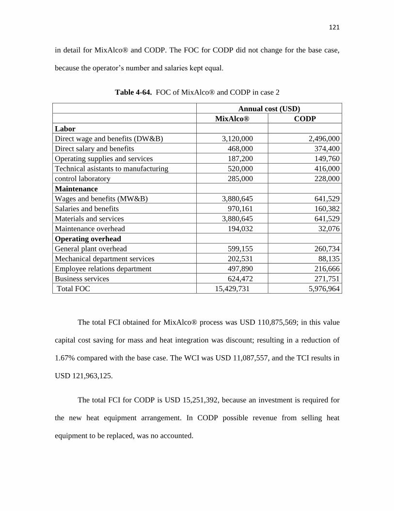
121

in detail for MixAlco® and CODP. The FOC for CODP did not change for the base case,

because the operator’s number and salaries kept equal.

Table 4-64. FOC of MixAlco® and CODP in case 2

Annual cost (USD)

MixAlco® CODP

Labor

Direct wage and benefits (DW&B) 3,120,000 2,496,000

Direct salary and benefits 468,000 374,400

Operating supplies and services 187,200 149,760

Technical asistants to manufacturing 520,000 416,000

control laboratory 285,000 228,000

Maintenance

Wages and benefits (MW&B) 3,880,645 641,529

Salaries and benefits 970,161 160,382

Materials and services 3,880,645 641,529

Maintenance overhead 194,032 32,076

Operating overhead

General plant overhead 599,155 260,734

Mechanical department services 202,531 88,135

Employee relations department 497,890 216,666

Business services 624,472 271,751

Total FOC 15,429,731 5,976,964

The total FCI obtained for MixAlco® process was USD 110,875,569; in this value

capital cost saving for mass and heat integration was discount; resulting in a reduction of

1.67% compared with the base case. The WCI was USD 11,087,557, and the TCI results in

USD 121,963,125.

The total FCI for CODP is USD 15,251,392, because an investment is required for

the new heat equipment arrangement. In CODP possible revenue from selling heat

equipment to be replaced, was no accounted.

122

Table 4-65 shows the obtained profitability results for MixAlco® process and

CODP, with and without the time value of money applying the integration mentioned in

this numeral.

Table 4-65. Summary MixAlco® and CODP economic results in case 2

MixAlco® with integration CODP with integration

Parameter Value Value


ROI estimated (%) 16.4 66,21

Annual gross (pre tax) profit (USD) 22,287,333 10,661,731

Annual net (after tax) profit (USD) 18,184,937 10,097,429

PBP (years) 3.56 1.28

Total operating cost (USD) 50,590,241 843,589,462

FCI (USD) 110,875,569 15,251,392

WCI (USD) 11,087,557 1,525,139

TCI (USD) 121,963,125 16,776,531


NPV (USD) 15,288,147 35,568,846

ROI real (%) 12.35 39.04

Annual sales (USD) 72,877,573 854,251,193

Tax rate (%) 35 35

Discount rate (%) 10 10

The retrofitting analysis in case 2 for MixAlco® process results in a ROI of 12.35%

acceptable in current market conditions; a ROI increment in 1.3% compared with the base

case. The NPV represent a profitable project of MM USD 15.3, with a NPV increment of




123


present dollars.

For this study case, CODP results in a ROI of 39% and a NPV of MM USD 35.6.

To compare the convenience of the retrofitting analysis in CODP, the profitability of CODP

integrated as a new plant was evaluated, as in the base case. The results show that CODP

integration had a reduction of ROI in 5.3%, and a NPV reduction in MM USD 0.80 was

obtained compared to the base case. The PBP for CODP is about 1.28 years assuming as a

new plant.

Figure 4-33. Cash flow of MixAlco® process in case 2

4.3.3.3 Comparison between cases

Table 4-66 shows the heat integration comparing the cases 1 and 2. For both cases,

the processes (MixAlco® and CODP) presented arrangements with operating cost savings.

124

Although in both cases there was a capital investment, the global economic evaluation

presented revenues.

Table 4-66. Heat integration comparison of cases

Base case

by joining

both plants

Case 1 Case 2

%

Difference

case 1

%

Difference

case 2

%

Difference

between

cases

Fired Heat (kJ/h) 1.41x108 8.25x107 1.10x108 ─ 71.0 % ─ 28.0 % 25.0 %

MP Steam (kJ/h) 4.13x108 4.08x108 4.07x108 ─1.00 % ─ 1.00 % 0%

Cooling Water (kJ/h) 1.98x108 1.44x108 1.50x108 ─ 38.0 % ─ 32.0 % 4.00 %

LP Steam (kJ/h) 4.90x106 2.73x106 2.79x106 ─79.0 % ─ 76.0 % 2.00 %

Refrigerant (kJ/h) 1.31x107 1.10x106 5.38x106 ─ 1.09 % ─ 143% 80.0 %

Heating (kJ/h) 5.59x108 4.94x108 5.20x108 ─ 13.0 % ─ 8.00 % 5.00 %

Cooling (kJ/h) 2.11x108 1.45x108 1.55x108 ─ 46.0 % ─ 36.0 % 6.00 %

Capital cost (USD) 2.29x107 2.83x107 3.21x107 19.0 % 29.0 % 12.0 %

Operating cost (USD/year) 1.28x107 1.03x107 1.13x107 ─ 24.0 % ─ 13.0 % 9.0 %

Table 4-67 shows the NPV and ROI for both retrofitting cases. For MixAlco®

process the ROI obtained in both cases is almost the same, but the NPV in case 1 is 2.6%

higher than in case 2. For CODP the ROI in case 1 is higher 2.8% than case 2, and the NPV

is 10% higher in case 1 than in case 2. Based on these results, it is possible to affirm that

case 1 is economically more profitable than case 2 for MixAlco® process and even more

for CODP.

Table 4-679. Economic comparison of cases

Case 1 Case 2

MixAlco® CODP MixAlco® CODP

NPV (MM USD) 15.7 39.2 15.3 35.6

ROI (%) 12.4 41.8 12.3 39.0

125

4.4 Sensitivity analysis

In this section, different variables were modified in order to study the behavior of the ROI

in each option. The understanding of the sensitivity analysis of the ROI helps in making the

optimal decision under given conditions.

4.4.1 Variation of gasoline prices

The first sensitivity analysis was based on the gasoline prices performance between

years 2010 to 2013 shown in Figure E-8 (Appendix E). The prices of gasoline were

changed from 2.5 to 3.8 USD per gallon.

Figure 4-34. Variation of gasoline price for MixAlco® process

For the best case of retrofitting and the base case, Figure 4-34 shows the result of

ROI and NPV of MixAlco® process for different gasoline prices. With limited ROI (5%)

the minimum selling price of gasoline is 2.7 USD per gallon. With a gasoline price of 3.8

126

USD per gallon the ROI obtained was 18%. From the NPV analysis, MixAlco® process

starts to be not profitable with gasoline price below 3.07 USD per gallon.

4.4.2 Variation of Jet prices

The second sensitivity analysis was based on the Jet prices performance between

years 2010 to 2013 shown in Figure E-7 (Appendix E). The prices of Jet were changed

from 2 to 3.8 USD per gallon.

Figure 4-35. Variaton of Jet price for MixAlco® process

For the best case of retrofitting and the base case, Figure 4-35 shows the result of

ROI and NPV of MixAlco® process for different Jet prices. Where, ROI does not reach the

minimum limit (5%). With a Jet price of 3.8 USD per gallon the ROI obtained was 15.8%.

From the NPV analysis, MixAlco® process starts to not be profitable with Jet price below

2.3 USD per gallon.

127

4.4.3 Variation of Biomass price

Based on the Pham et al., (2012) study, the price of biomass feedstock could be

changed from 20 to 120 USD per ton. Figure 4-36 shows the variation of Biomass prices

from 0 to 120 USD per ton. When the price of biomass is free, the ROI is 21.5%,

maintaining the MixAlco® plant capacity of 60 ton/h. Also, Figure 4-36 shows the

maximum price of Biomass in 73 USD/ton in order to have the NPV positive and the

project will be profitable.

Figure 4-36. Variation of Biomass price

4.4.4 Variation of MixAlco® plant capacity

The fourth sensitivity analysis was based on the MixAlco® plant capacity, varying

the biomass feedstock from 20 to 160 ton/h. To do that, the FCI was calculated using the

six tenths factor rule explained in Appendix E, with a scaling factor of 0.6, according to the

128

literature (Pham et al., 2010). The consumption of utilities and chemicals had been

calculated, and the annual sales should be adjusted for each capacity. In this analysis the

biomass price was constant in 60 USD/ton.

For the best retrofitting case, Figure 4-37 shows the result of ROI and NPV varying

the MixAlco® plant capacity. From the NPV analysis, MixAlco® process starts to be

profitable with an approximated 33 ton/ h of capacity. With a MixAlco® plant capacity

above 70ton/h was provided a ROI higher than 20%.

Figure 4-37. Variation of MixAlco® plant capacity

129

5 CONCLUSIONS

In order to evaluate the retrofitting analysis to integrate the MixAlco® process to the

crude oil distillation process (CODP), this work was developed in four stages. The first

stage was the building of each process (as a base case) with mass and energy balances and

economical evaluation. In this way, a simulation of the entire MixAlco® process was made.

This simulation used a feedstock stream (sugarcane bagasse/chicken manure) of

40ton/h, using ketonization process route. The results obtained for MixAlco® simulations

were the expected, according to literature (Pham et al., 2012), (Gosseaume, 2011),

(Holtzapple, 2004), (Pham, Holtzapple, & El-Halwagi, 2012). Also, a typical crude oil

distillation process for commercial crude oil with 22.4API was simulated with preheating

trains and atmospheric/vacuum units. In the second stage, the hierarchical methodology

proposed was used as a strategy to achieve cost-effective studies through profitability

analysis. Different levels for applying the hierarchical methodology were done:

- Internal rearrangements within each process, where it was obtained only a mass

integration within MixAlco® process. Considering, recycle water from dewatering unit to

fermentation and pretreatment units. The base case of MixAlco® was obtained with a ROI

of 11.1% and a NPV of MM USD 7.3. The base case of CODP was obtained with a ROI of

31.2% and a NPV of MM USD 29 as a new plant.

- Internal modifications within each process, where heat integration within each plant

was made. For MixAlco® the heating and cooling utility load, results reduced in 8.3% the

capital cost and in 8.6% the operating cost. Also, it was obtained a ROI of 11.8% and a

NPV of MM USD 11.7. For CODP the heating and cooling utility load, reduced in 39%

130

the operating cost but increased a capital cost 78%. In this case CODP obtained a ROI of

41.8% and a NPV of MM USD 39.2.

- External modification through retrofitting analysis between MixAlco® process

and CODP, where two relevant cases where analyzed and compared. The first case was

based on a mass and heat integration within each process. Also, water integration between

both plants was made. The economical results were a 12.4% of ROI, and MM USD 15.7 of

NPV for MixAlco® process. The second case was based on integration of both plants,

where MixAlco® process was added to CODP with heat integration inside the plant.

Results presented a ROI of 12.35% and NPV of MM USD 15.3 for MixAlco® process.

The third stage was the comparison between the two cases mentioned above, where

the case 1 resulted in the best retrofitting analysis. There was an NPV increment from MM

USD 7.3 to MM USD 15.7, and ROI increment from 11.1% to 12.4% for MixAlco®

process. According to retrofitting results, it is necessary to make an investment in capital

cost of MM USD 15 for CODP that will be payback in 15 months (according to

profitability analysis).

The fourth stage was a sensitivity analysis to MixAlco® process for the best

retrofitting case. The mainly results for MixAlco® be profitable were a minimum gasoline

price of 3.07 USD per gallon, and a minimum Jet price of 2.3 USD per gallon. Besides,

with the maximum price of gasoline or Jet (3.8 USD per gallon) an obtained ROI was 18%

and 15.8% respectively. For a MixAlco® plant capacity of 60 ton/h was obtained a ROI of

21.5% if the biomass price was free; and the maximum price of biomass was 73 USD/ton in

order to have the NPV positive and the project will be profitable. Finally, MixAlco®

131

process starts to be profitable from about 33 ton/ h of capacity. For a MixAlco® capacity

above 70ton/h was obtained ROIs above 20%.

132

6. RECOMMENDATIONS AND FUTURE WORK

After completing this work, it is considered important to research in future works

into the optimization of the mixture of both products (bio-gasoline / gasoline), in order to

optimize the retrofitting analysis.

It is considered important to study in future works the plant capacity of MixAlco®

and CODP, getting a better compatibility in the Pinch point.

It is recommended to study a case of both plants (MixAlco® and CODP) as news,

different that was done in this work, and compare the cases.

In order to verify the MixAlco® process simulation is recommended validate it with

Terrabon, the demostration plant of MixAlco® located in College Station, Texas.

It is recommended to study in future works different ways of heat integration, for

example study the integration of syngas from MixAlco® with the furnace located in the

atmospheric unit of CODP. Moreover, study other types of heat exchangers as compact

heat exchangers. Otherwise, include the fouling affectation in the preheating system with

the time.

It is also considered important to include in future works, the study of life cycle

analysis (LCA) into a bio-refinery retrofitting analysis, in order to evaluate the greenhouse

gas emissions (GHG) and associate it with the economic evaluation by Clean Development

Mechanism (CDM).

Furthermore, it is recommended to investigate the retrofitting analysis on other

products, in order to integrated biofuels into the existing fossil-based process.

133

Finally, it is recommended to develop a computational template which integrates all

calculations of integration, technical and economic analysis and the selection of the best

alternative.

134

REFERENCES

Aspen plus®. (2013). Software database and help menu (Version 7.3).

Benali, T., & Tondeur, J. N. (2011). An improved crude oil atmospheric distillation process

for energy integration: Part I: Energy and exergy analyses of the process when a

flash is installed in the preheating train. Applied Thermal Engineering. 125 -131.

Cormier, B. (2005). Retrofitting Analysis of Integrated Bio-refineries. Texas A&M

University, College Station, TX.

EIA. (2013, July 9). Retrieved 2013, 13-July from the U.S. Energy Information

Administration: http://www.eia.gov/forecasts/steo/report/global_oil.cfm

EIA. (2013, July 15). Retrieved 2013, 10-June from the U.S. Energy Information

Administration: http://www.eia.gov/dnav/pet/hist/LeafHandler.ashx?n=PET&s=

EMM_EPMRU_PTE_R30_DPG&f=W

El-Halwagi, M. (2012). Sustainable design through process integration. Texas: Elsevier.

El-Halwagi, M., & Spriggs, H. D. (1998). Solve Design Puzzles with Mass Integration.

Chemical engineering progress, 8(94), 25-44.

Felder, R., & Rousseau, R. (2005). Elementary principles of chemical processes. Atlanta:

John Wiley & Sons, Inc.

Fernández, J. (2007). Diseño de un modelo de optimización de la planta de crudo de

Ecopetrol S.A. en la Refinería de Cartagena. Magister thesis in Industrial

Engineering. Bogotá.

135

Gosseaume, P. (2011). Development of a simulation tool of the MixAlco Technology to be

applied in Colombia. Grenoble INP-Pagora, France.

Granda, C., Holtzapple, M., Luce, G., Searcy, K., & Mamrosh, D. (2009). Carboxylate

Platform: The MixAlco Process Part 2: Process Economics. Appl Biochem

Biotechnol, 537 - 554.

Holtzapple, M. (2004). MixAlco Process: Biomass to Carboxylic Acids and Alcohols.

College Station, TX.

Holtzapple, M. (2009). Patent application 'Methods and Systems for Biomass Conversion

to Carboxylic Acids and Alcohols'.

Peters, M., Timmerhaus, K., & West, R. (2004). Plant Design and Economics for Chemical

Engineers. 5th Edition. Colorado: Mc Graw Hill.

Pham, V., Holtzapple, M., & El-Halwagi, M. (2010). Techo-economic analysis of biomass

to fuel conversion via the MixAlco process. J Ind Microbiol Biotechnol.

Pham, V., Holtzapple, M., & El-Halwagi, M. (2012). Chapter 6. Technoeconomic Analysis

of a Lignocellulose-to-Hydrocarbons Process Using a Carboxylate Platform.

Integrated Biorefineries: Design, Analysis, and Optimization (Green Chemistry and

Chemical Engineering) (p. 157 - 192). Texas. Chapman & Hall.

Seider, W., Seader, J. D., & Lewin, D. (2004). Product & Process Design Principles. 2nd

Edition. Wiley.

136

Sierra, R., García, L., & Holtzapple, M. (2010). Selectivity and Delignification Kinetics for

Oxidative and Nonoxidative Lime Pretreatment of Poplar Wood, Part III: Long-

Term. AIChE.

Terrabon. (2010, October). Retrieved 2010, 12-October from:

http://www.terrabon.com/mixalco_economics.html

Towler, G., & Sinnott, R. (2013). Chapter 7. Capital Cost Estimating. Chemical

Engineering Design (págs. 307 - 351). Elsevier.

Wooley, R., & Putsche, V. (1996). Development of an Aspen Plus Physical Property

Database for Biofuels Components. Golden, Colorado.

Zhihong, F., & Holtzapple, M. (2010). Fermentation of Sugarcane Bagasse and Chicken

Manure to Calcium Carboxylate under Thermophilic Conditions. Appl Biocehm

Biotechnol, 561-578.

137

APPENDIX A

A.1 Literature review

A.1.2 MixAlco® Process Description

The MixAlco® process is a robust process that converts biomass to fuels and chemicals. A

key feature of the MixAlco® process is the fermentation, which employs a mixed culture of

acid-forming microorganisms to convert biomass components (carbohydrates, proteins, and

fats) to carboxylate salts. Subsequently, these intermediate salts are chemical converted to

hydrocarbon fuels (gasoline, jet fuel, and diesel). (Pham et al., 2010)

Figure A-1 shows biomass-to-hydrocarbon fuels conversion via ketonization. To make

hydrocarbon fuels, the MixAlco® process uses the following steps: (I) pretreatment with

lime, (II) fermentation with a mixed culture of acid-forming microorganism to obtain

carboxylate salts, (III) dewatering using a high-efficiency vapor-compression evaporator,

(IV) thermal conversion of salts to ketones (V) hydrogenation of the ketones to mixed

alcohols, and (VI) oligomerization of alcohols to hydrocarbons using zeolite catalysts.

(Pham et al., 2010)

138

Figure A-1. MixAlco® process via Ketonization. (Pham et al., 2010)

The biomass feedstock must contain a source of energy and a source of nutrients.

Examples of energy sources include sorghum, bagasse, municipal solid waste, office paper,

paper fines, rice straw, water hyacinths, pineapple waste, and aloe-vera pulp. Examples of

nutrient sources include food scraps, sewage sludge, and manure. In addition, chemical

nutrients (e.g., urea, ammonia, ammonium bicarbonate) can be added to supply essential

minerals. (Pham et al., 2010)

FEED HANDLING

Figure A-2 shows a schematic of the loading facilities. Screw conveyor A-2 augers

quick lime (CaO) into mixer A-3, which blends biomass, quick lime, water, and calcium

carbonate. The quick lime reacts with water, releasing heat which raises the temperature of

the mixture. The biomass/lime/water/calcium carbonate mixture is fed to loader A-1, which

stores a few hundred tons of the mixture. (Holtzapple, 2004)

139

Figure A-2. Schematic of loading facilities. (Holtzapple, 2004)

PRETREATMENT AND FERMENTATION

Different forms of pretreatment exist, using physical, chemical or biological means.

It has been found hat pretreatment with lime and air efficiently delignifies lignocellulosic

materials, increasing digestibility significantly. This type of pretreatment is preferred over

other pretreatment options for the MixAlco® process because it is best integrated with

further processing and recovery steps. (Gosseaume, Development of a simulation tool of

the MixAlco® Technology to be applied in Colombia, 2011)

Recycled lime from the lime kiln is assumed to contribute 85% of lime demand in

the pretreatment, with the 15% make-up lime purchased from external vendors. Although

the residence time of pretreatment (6 weeks) and fermentation (8 weeks) is long, the round-

robin system results in steady flow rate and product concentration in the broth. (Pham et al.,

2010)

140

An example of the pretreatment/fermentation piles operated in a round-robin

manner is presented in figure A3, where there are six piles, two pretreatment and four in

fermentation. As the lime pretreatment pile ages, the pH drops. Then the air is shut off, and

the inoculum is added, so it becomes a fermentation pile. When the fermentation is

complete, the residue is removed, and pretreatment starts with a new pile. Figure A4 shows

the water circulation pattern while in the fermentation mode. (Granda, Holtzapple, Luce,

Searcy, & Mamrosh, 2009)

Figure A-3. Round - robin system. (Granda et al., 2009)

Figure A-4. Water circulation through the piles. (Granda et al., 2009)

Figure A-5 shows the pile in the pretreatment mode. A blower (A-5) pressures air

and blows it through a lime-water slurry tank (A-6), which removes carbon dioxide from

the air. The air then blows up through the pile, which contains both biomass and lime. The

Most digested biomass

6

5 4 Freshest biomass

3

141

pile is located on a gravel bed lined with a geomembrane. Water accumulates in the gravel

bed and is circulated to the top of the pile. The combination of lime, water, and air removes

lignin from the biomass, rendering it digestible. During the pretreatment mode, the pile can

be covered or uncovered. If covered, an exhaust blower (A-7) removes gas from the pile. A

slight vacuum can be created, which keeps the cover pressed against the pile thereby

keeping it from blowing in the wind. Liquid collected from the bottom of the pile is

pumped (A-8) through a heat exchanger (A-9) onto the top of the pile. (Granda et al., 2009)

Figure A-5. Pretreatment pile. (Granda et al., 2009)

Once the lime is consumed within the pile, the pH will drop. At this point, the pile is

inoculated with a mixed culture of acid-forming microorganisms that digest the biomass

and form volatile fatty acids (VFAs) such as acetic, propionic, and butyric acids. The VFAs

react with the calcium carbonate within the pile, thus forming salts of the VFAs, such as

142

calcium acetate, propionate, and butyrate. Because they tolerate high salt concentrations,

the best source of the inoculum is from saline environments. (Holtzapple, 2004)

Holtzapple, (2004) show in Figure A-6 the pile in the fermentation mode. In this

case, no air circulates through the pile and the exhaust gases are sent to a packed bed

scrubber (A-10) where they contact ammonia and water to form ammonium bicarbonate

buffer for our case the buffer is calcium carbonate, which is stored in a holding tank (A-11)

and directed to the liquid that circulates through the pile. Gases exiting the scrubber (A-10)

are sent to an odor control system (A-12) if no hydrogen is present in the gas. If hydrogen

is present, then the gas is sent to a hydrogen recovery unit (not shown).

Figure A-6. Pile in Fermentation form. (Granada et al., 2009)

Figure A-7 shows that after the fermentation is completed, the pile is dismantled by

slurrying the undigested residue with water (A-14) and pumping (A-13) the slurry through

143

a filter (A-16). The undigested residue can be sent to a boiler to make process heat, a

gasifier to make hydrogen, or it can be exported for other purposes (compost, electricity

production). (Granada et al., 2009)

Figure A-7. Dismantling the fermentation pile. (Granada et al., 2009)

Biomass is composed of volatile solids (VS) and ash. Most of the VS are reactive

except lignin, whereas the ash content is nonreactive. Mass balances closure is performed

during steady-state countercurrent fermentations. Figure A-8 illustrates a typical

fermentation process, which converts VS into gas and liquid products, with some solids

remaining undigested. (Zhihong & Holtzapple, 2010).

144

Figure A-8. Digestion of biomass. (Zhihong & Holtzapple, 2009)

DESCUMMING AND DEWATERING

In the produced fermentation broth, the calcium carboxylate concentration is 6%

weight. Other components (e.g., dissolved carbon dioxide, microorganisms, undigested

biomass, and other unknowns) are impurities and must be removed along with water. To

purify the carboxylate salts, the broth is degasified by stripping, descummed using

flocculant, evaporated using vapor compression, and crystallized (Figure A-9). (Pham et al.,

2010)

Figure A-9. Simplified process block of the descumming and dewatering units. (Pham et

al., 2010)

KETONIZATION AND LIME KILN

The solid salts are sent to a dryer to remove residual moisture (Figure A-10). At

high temperatures (430°C) in the ketonization reactor, calcium carboxylates are thermally

145

converted into ketones and calcium carbonate. The reactor is kept under vacuum (30

mmHg), which reduces residence time to avoid decomposition of the produced ketones.

The ketone vapor is quickly removed from the reactor, quenched, and condensed. (Pham et

al., 2010)

Figure A-10. Simplified process block of the ketonization and lime kiln unit. (Pham et al.,

2010)

The general ketonization reaction is represented as following:

Carboxylate calcium Ketone Calcium carbonate

Part of the calcium carbonate is directly recycled to the fermentors, and the remaining

portion is converted into quick lime (CaO) in a kiln. The quick lime is recycled to the

pretreatment reactors. Unlike conventional lime kilns that are fed coarse limestone, this kiln

processes fine calcium carbonate powder; thus, some processing steps (grinding, drying)

are not needed. This reaction takes place at 900°C or 1000°C. (Pham et al., 2010)

KETONE HYDROGENATION

In this conversion step, the ketone carbonyl groups react with hydrogen to form

alcohol groups in an exothermic reaction:

146

Ketone Hydrogen Alcohol

The reaction is performed at high pressure (55 bar) and at isothermal (130°C)

condition. The optimal design was found to be three continually stirred tank reactors

(CSTR) in series. In each CSTR, liquid ketones, solid Raney nickel catalyst, and hydrogen

bubbles are well mixed. The heat of reaction is recovered by a pump-around system.

Hydrogen is fed to every CSTR in 20%excess to maximize ketone conversion. The net

demand of hydrogen is 0.0225 kg H2/kg mixed alcohol [25.0 standard cubic foot (SCF) per

gallon of mixed alcohols] or 0.00687 kg H2/kg dry ash-free biomass (1.30 SCF per dry ash-

free pound of biomass). The produced mixture of secondary alcohols can be directly used

as a transportation oxygenated fuel such as bioethanol, but it has higher energy content (net

heating values are 34.6 and 26.8 MJ/kg, respectively. (Pham et al., 2010)

DEHYDRATATION AND OLIGOMERIZATION

The mixed alcohols are further processed to produce hydrocarbon fuels. Using H-

ZSM-5 catalyst in a reactor at 300°C and 3 bar, the alcohols are dehydrated as follows:

Alcohol Olefins Water

In the same reactor, the produced olefins are oligomerized as shown in the

following simplified reaction:

Olefins Longer Olefins

147

Depending upon the specific reaction conditions (time, pressure, temperature) the

products are very complex and include olefins, n-paraffins, iso-paraffins, aromatics, and

cyclics. Water in the products is removed in a drying unit using a salt filter. (Pham et al.,

2010)

OLEFIN HYDROGENATION

To improve fuel quality, the olefins can be hydrogenated to make corresponding

paraffins. Similar to the design of the ketone hydrogenation, this conversion unit employs

CSTRs in series with Raney nickel catalyst. The carbon double bond (C=C) is saturated to

stabilize the hydrocarbon product as follows:

Olefins Paraffins

In this step, the net demand of hydrogen is 0.0139 kg H2/kg hydrocarbon fuels (15.4

SCF per gallon of hydrocarbon fuel) or 0.0034 kg H2/kg dry ash-free biomass (0.64 SCF

per dry ash-free pound of biomass). (Pham et al., 2010)

Out of the reactor, the mixed hydrocarbons are distilled into C8- and C9+ fractions.

The light fraction and heavy components can be used as blending components for gasoline

and jet fuel, respectively. (Pham et al., 2010)

148

GASIFICATION

Hydrogen is required to produce alcohols and saturate hydrocarbons. This hydrogen

is produced by gasifying undigested biomass from the fermenters. (Pham et al., 2010)

STEAM-GAS SHIFT AND PRESSURE-SWING ADSORPTION

More hydrogen is made using the shift reaction between steam and carbon

monoxide. Because of the compositional characteristics of the syngas, a one-stage shift is

sufficient for high conversion and low residence time. The hydrogen-rich syngas, along

with fermentation gas, is passed through molecular sieve beds in the pressure-swing

adsorption unit, which purifies hydrogen. (Pham et al., 2010)

A.2 Consideration in MixAlco® Process Simulation

A.2.1 Fermentation

Biomass to Sugar

(Eq. A-1)

Cellulose Glucose

(Eq. A-2)

Xylan Xylose

Sugar to Acid

(Eq. A-3)

Glucose Acid acetic

(Eq. A-4)

Glucose Acid propionic

(Eq. A-5)

Glucose Acid valeric

(Eq. A-6)

Xylose Acid acetic

149

(Eq. A-7)

Xylose Acid propionic

(Eq. A-8)

Xylose Acid valeric

Acid neutralization

(Eq. A-9)

Acid acetic Calcium acetate

(Eq. A-10)

Acid propionic Calcium propionate

(Eq. A11)

Acid valeric Calcium pentanoate

Table A-1. Conversion factors in fermentation reactors

Reactions R-102 R-103 R-104 R-105

1 CELLU-01(Cisolid) + WATER --> GLUCO-01 0.3823 0.4741 0.517 0.542

2 XYLAN(Cisolid) + WATER --> XYLOS-01 0.3823 0.4741 0.517 0.542

3 GLUCO-01 --> 3 A-ACETI 0.840 0.840 0.840 0.840

4 GLUCO-01 --> 2 A-PROP + .727 CO2 0.0500 0.0500 0.0500 0.0500

5 5 GLUCO-01 --> 6 A-VAL + 6.543 CO2 1.00 1.00 1.00 1.00

6 2 XYLOS-01 --> 5 A-ACETI 0.800 0.800 0.800 0.800

7 3 XYLOS-01 --> 5 A-PROP + 1.818 CO2 0.250 0.250 0.250 0.250

8 XYLOS-01 --> A-VAL + 1.09 CO2 1.00 1.00 1.00 1.00

9 2 A-ACETI + CACO3(Cisolid) --> WATER +

CO2 + CA(CH-01(Cisolid)

1.00 1.00 1.00 1.00

10 2 A-PROP + CACO3(Cisolid) --> CA(CH-

02(Cisolid) + WATER + CO2

1.00 1.00 1.00 1.00

11 2 A-VAL + CACO3(Cisolid) --> CA(CH-

03(Cisolid) + WATER + CO2

1.00 1.00 1.00 1.00

A.2.2 Ketonization

Carboxylate salts to ketone

(Eq. A-12)

Calcium acetate Acetone

150

(Eq. A-13)

Calcium acetate Calcium propionate Butanone (or Methyl-ethyl ketone)

(Eq. A14)

Calcium acetate Calcium pentanoate 2-hexanone (or methyl buthyl ketone)

(Eq. A-14)

Calcium propionate 3-pentanone

(Eq.A15)

Calcium propionate Calcium pentanoate 3-heptanone

(Eq. A-16)

Calcium pentanoate 5-nonanone

Ketone to Alcohol

(Eq. A-17)

Acetone Isopropanol

(Eq. A-18)

Butanone Sec-butanol (or 2-butanol)

(Eq. A-19)

2-hexanone 2- hexanol

(Eq. A-20)

3-pentanone 3- pentanol

(Eq. A-21)

3-heptanone 3- heptanol

(Eq.A22)

5-nonanone 5-nonanol

A.2.3 FINAL

Dehydratation

(Eq. A-23)

Isopropanol C3H6 = Propylene

(Eq. A-24)

2-butanol C4H8 = 2-butene

151

(Eq. A-25)

2- hexanol C6H12 = 2-hexene

(Eq. A-26)

3- pentanol C5H10= 2-pentene

(Eq. A-27)

3- heptanol C7H14 = 1,2-dimethylcyclopentane

(Eq. A-28)

5-nonanol C9H18 = 2-nonene

Oligomerization

(Eq. A-29)

Propylene + 2-butene 1,2-dimethylcyclopentane

(Eq. A30)

Propylene +2-pentene 1,2-dimethylcyclohexane

(Eq. A31)

Propylene +2-hexene 2-nonene

(Eq. A-32)

Propylene + 1,2-dimethylcyclopentane 1,4-diethylcyclohexane

(Eq. A-33)

Propylene + 1,2-dimethylcyclohexane undecene

(Eq. A-34)

Propylene + 2-nonene 1-dodecene

(Eq. A-35)

2-butene + 2-pentene 2-nonene

(Eq. A-36)

Propylene+ Propylene 2-hexene

Olefin hydrogenation

(Eq. A-37)

2-butene butane

152

(Eq. A-38)

2-pentene pentane

(Eq. A-39)

2-hexene hexane

(Eq. A-40)

1,2-dimethylcyclopentane heptane

(Eq. A-41)

1,2-dimethylcyclohexane octane

(Eq. A-42)

2-nonene nonane

(Eq. A-43)

1,4-diethylcyclohexane decane

(Eq. A-44)

undecene undecane

(Eq. A-45)

1-dodecene dodecane

Table –A-2. Conversion factor for reactor R-111

Oligomerization Conversion

C3H6 + C4H8 --> C7H14 0.2

C3H6 + C5H10 --> C8H16 0.4

C3H6 + C6H12 --> C9H18 0.7

C3H6 + C8H16 --> C11H22 0.2

C3H6 + C9H18 --> C12H24 0.2

C4H8 + C5H10 --> C9H18 0.4

C5H10 + C6H12 --> C11H22 0.95

2 C3H6 --> C6H12 0.5

153

APPENDIX B

Table B-1. Components List in MixAlco® simulation (Gosseaume, 2011)

Component ID Type Component name Formula

CELLU-01 SOLID CELLULOSE C6H10O5

XYLAN SOLID XYLAN C5H8O4

LIGNI-01 SOLID LIGNIN CXHXOX

BIOMA-01 SOLID BIOMASS CHXNXOXSX-1

GLUCO-01 CONV GLUCOSE C6H12O6

XYLOS-01 CONV XYLOSE C5H10O5

SOLSL-01 CONV SOLSLDS CHXOXSX

SOLUN-01 CONV SOLUNKN CXHOX

WATER CONV WATER H2O

AIR CONV AIR AIR

CO CONV CARBON-MONOXIDE CO

CO2 CONV CARBON-DIOXIDE CO2

CA(OH)2 SOLID CALCIUM-HYDROXIDE CA(OH)2

CACO3 SOLID CALCIUM-CARBONATE-CALCITE CACO3

CA(CH-01 SOLID CA(CH3CO2)2 CAC4H6O4

CA(CH-02 SOLID CA(CH3CH2CO2)2 CA(PROP)2

CA(CH-03 SOLID CA(CH3CH2CH2CH2CO2)2 CA(PENT)2

NITROGEN CONV NITROGEN N2

O2 CONV OXYGEN O2

CAO SOLID CALCIUM-OXIDE CAO

A-ACETI CONV ACETIC-ACID C2H4O2-1

A-PROP CONV PROPIONIC-ACID C3H6O2-1

A-VAL CONV N-VALERIC-ACID C5H10O2-1

HYDROGEN CONV HYDROGEN H2

ACETONE CONV ACETONE C3H6O-1

BUTANONE CONV METHYL-ETHYL-KETONE C4H8O-3

HEXANONE CONV 2-HEXANONE C6H12O-D3

PENTANON CONV DIETHYL-KETONE C5H10O-4

HEPTANON CONV 3-HEPTANONE C7H14O-E1

NONANONE CONV 5-NONANONE C9H18O-E2

ISOPROPA CONV ISOPROPYL-ALCOHOL C3H8O-2

BUTANOL CONV 2-BUTANOL C4H10O-2

HEXANOL CONV 2-HEXANOL C6H14O-E1

PENTANOL CONV 3-PENTANOL C5H12O-D4

HEPTANOL CONV 3-HEPTANOL C7H16O-D4

NONANOL CONV 1-NONANOL C9H20O-D2

1-BUT-01 CONV 1-BUTENE C4H8-1

C3H6 CONV PROPYLENE C3H6-2

C4H8 CONV CIS-2-BUTENE C4H8-2

C5H10 CONV TRANS-2-PENTENE C5H10-4

C6H12 CONV TRANS-2-HEXENE C6H12-5

C7H14 CONV TRANS-1,2-DIMETHYLCYCLOPENTANE C7H14-4

C9H18 CONV TRANS-2-NONENE C9H18-D5

154

Component ID Type Component name Formula

C8H16 CONV TRANS-1,2-DIMETHYLCYCLOHEXANE C8H16-3

C10H20 CONV TRANS-1,4-DIETHYLCYCLOHEXANE C10H20-D7

C11H22 CONV 1-UNDECENE C11H22-2

C12H24 CONV 1-DODECENE C12H24-2

C13H26 CONV 1-TRIDECENE C13H26-2

C4H10 CONV N-BUTANE C4H10-1

C5H12 CONV N-PENTANE C5H12-1

C6H14 CONV N-HEXANE C6H14-1

C7H16 CONV N-HEPTANE C7H16-1

C8H18 CONV N-OCTANE C8H18-1

C9H20 CONV N-NONANE C9H20-1

C10H22 CONV N-DECANE C10H22-1

C11H24 CONV N-UNDECANE C11H24

C12H26 CONV N-DODECANE C12H26

C13H28 CONV N-TRIDECANE C13H28

C12H24 CONV 1-DODECENE C12H24-2

C13H26 CONV 1-TRIDECENE C13H26-2

155

Table B2. Components properties for MixAlco® process. (Aspen plus®, 2013)

COMPONENT API DHFORM (kJ/mol) MW SG TBP

(°C) ZC

VLSTD

(cm3/mol)

CELLU-01 -3.6 -1,022.0 162.1 1.1 215.9 0.28 147.0

XYLAN -20.9 -842.6 132.1 1.3 322.4 0.22 103.5

GLUCO-01 -11.9 -1,089.0 180.2 1.2 343.9 0.32 152.6

WATER 10.0 -241.8 18.0 1.0 100.0 0.23 18.1

AIR 28.9 0.0 29.0 0.9 -194.5 0.31 32.9

CO 340.0 -110.5 28.0 0.3 -191.5 0.30 53.6

CO2 340.0 -393.5 44.0 0.3 -78.5 0.27 53.6

NITROGEN 340.0 0.0 28.0 0.3 -195.8 0.29 53.6

O2 340.0 0.0 32.0 0.3 -183.0 0.29 53.6

A-ACETI 2.6 -432.8 60.1 1.1 117.9 0.21 57.6

A-PROP 10.1 -453.5 74.1 1.0 141.2 0.22 74.3

A-VAL 18.4 -490.1 102.1 0.9 185.8 0.24 108.4

HYDROGEN 340.0 0.0 2.0 0.3 -252.8 0.31 53.6

ACETONE 48.5 -215.7 58.1 0.8 56.3 0.23 74.0

BUTANONE 43.4 -239.0 72.1 0.8 79.6 0.25 89.3

HEXANONE 43.4 -279.8 100.2 0.8 127.6 0.25 124.1

PENTANON 42.9 -257.9 86.1 0.8 102.0 0.27 106.4

HEPTANON 41.9 -301.0 114.2 0.8 147.4 0.25 140.3

NONANONE 41.2 -344.9 142.2 0.8 188.5 0.24 174.0

ISOPROPA 47.8 -272.1 60.1 0.8 82.2 0.25 76.3

BUTANOL 43.1 -292.9 74.1 0.8 99.8 0.25 91.6

HEXANOL 42.7 -334.6 102.2 0.8 139.3 0.26 126.1

PENTANOL 41.3 -315.4 88.1 0.8 115.3 0.26 107.9

HEPTANOL 40.5 -352.5 116.2 0.8 156.0 0.27 141.6

NONANOL 39.7 -377.9 144.3 0.8 212.1 0.26 175.0

1-BUT-01 103.8 -0.5 56.1 0.6 -6.2 0.28 93.6

C3H6 139.6 20.2 42.1 0.5 -47.7 0.28 80.9

C4H8 94.1 -7.4 56.1 0.6 3.7 0.27 89.7

C5H10 85.0 -31.1 70.1 0.7 36.3 0.27 107.6

C6H12 75.8 -53.8 84.2 0.7 67.9 0.26 123.6

C7H14 55.6 -136.7 98.2 0.8 91.9 0.27 130.2

C9H18 61.9 -109.7 126.2 0.7 150.1 0.25 173.0

C8H16 49.9 -180.0 112.2 0.8 123.4 0.27 144.2

C10H20 45.8 -214.7 140.3 0.8 176.3 0.28 176.2

C11H22 56.1 -144.9 154.3 0.8 192.7 0.25 205.0

C12H24 54.1 -165.4 168.3 0.8 213.0 0.25 221.3

C13H26 52.4 -186.2 182.3 0.8 232.8 0.25 237.6

156

COMPONENT API DHFORM (kJ/mol) MW SG TBP

(°C) ZC

VLSTD

(cm3/mol)

C4H10 110.6 -125.8 58.1 0.6 -0.5 0.27 99.7

C5H12 92.8 -146.8 72.2 0.6 36.1 0.27 114.7

C6H14 81.6 -166.9 86.2 0.7 68.7 0.27 130.1

C7H16 74.1 -187.6 100.2 0.7 98.4 0.26 146.0

C8H18 68.7 -208.7 114.2 0.7 125.7 0.26 162.0

C9H20 64.6 -228.7 128.3 0.7 150.8 0.26 178.2

C10H22 61.2 -249.5 142.3 0.7 174.2 0.25 194.3

C11H24 58.6 -270.4 156.3 0.7 195.9 0.25 210.5

C12H26 56.5 -290.7 170.3 0.8 216.3 0.25 226.9

C13H28 54.6 -311.8 184.4 0.8 235.5 0.25 243.1

CACO3 0.0 100.1 0.20

CA(CH-02 186.2

CA(CH-03 242.3

CA(OH)2 -610.8 74.1 0.20

CAO 43.9 56.1 3,396.9 0.20

CA(CH-01 158.2

XYLOS-01 -1,040.0 150.1 441.9

SOLSL-01 -47.5 16.6 552.3

SOLUN-01 -119.0 15.0 552.3

LIGNI-01 122.5

BIOMA-01 23.2

The properties shown in Table C2 are:

DHFORM: Formation Enthalpy

TBP: True Normal Boiling Point

ZC: Critical Compressibility Factor

VLSTD: Standard Liquid Molar Volume at 60°F

SG: Standard Specific Gravity at 60°F

MW: Molecular Weight

API: Standard API gravity

157

APPENDIX C

C.1 Mass Integration Literature review

Several mass integration strategies can be used to develop cost-effective

implementations. These strategies include stream segregation/mixing, recycle, interception

using separation devices, changes in design and operating conditions of units, materials

substitution, and technology changes including the use of alternate chemical pathways.

These strategies can be classified into a hierarchy of three categories shown in Figure C-1:

no-/low-cost changes, moderate cost modifications, and new technologies. (El-Halwagi,

2012)

Figure C-1. Hierarchy of mass-integration strategies. (El-Halwagi, 2012)

C.1.1 Mass Integration Targeting

Three sets of data for that species are first collected: fresh usage, terminal discharge,

and generation/depletion. The fresh usage (F) refers to the amount of the targeted species in

the streams entering the process (the waste stream may have entered the process as a fresh

feedstock or a material utility). The terminal discharge (T) corresponds to the load of the

targeted species in streams designated as waste streams or point sources for pollution.

158

Generation (G) refers to the net amount of the targeted species, which is produced through

chemical reaction. Depletion (D) may take place through chemical reactions but it may also

be attributed to leaks, fugitive emissions, and other losses that are not explicitly accounted

for. The net generation (Net_G) of a targeted species is defined as the difference between

generation (G) and depletion (D). Superscripts indicate the stated of the stream, AMI

means after mass integration, AFR after reduction that means the minimum load of the

targeted species, AGMIN means after minimization of net generation.

To minimize the terminal discharge of the targeted species, we should recycle the

maximum amount from terminal streams (or paths leading to terminal streams) to replace

fresh feed.

When the target is minimize the fresh usage then the net generation must be

maximize, like in Figure C-2, but when the target is minimize the waste discharge, the net

generation must be minimum, and the Figure C-2 is different for minimize the net

generation. The third case that can be present is when the net generation is no altered, then

the target procedures for minimize waste discharge or fresh usage become identical. (El-

Halwagi, 2012)

Figure C-2. Targeting for minimum usage of material utilities. (El-Halwagi, 2012)

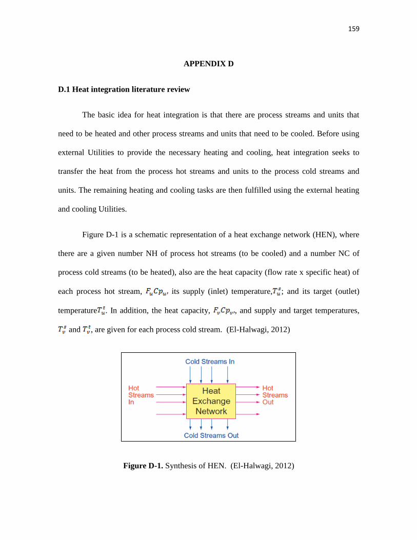
159

APPENDIX D

D.1 Heat integration literature review

The basic idea for heat integration is that there are process streams and units that

need to be heated and other process streams and units that need to be cooled. Before using

external Utilities to provide the necessary heating and cooling, heat integration seeks to

transfer the heat from the process hot streams and units to the process cold streams and

units. The remaining heating and cooling tasks are then fulfilled using the external heating

and cooling Utilities.

Figure D-1 is a schematic representation of a heat exchange network (HEN), where

there are a given number NH of process hot streams (to be cooled) and a number NC of

process cold streams (to be heated), also are the heat capacity (flow rate x specific heat) of

each process hot stream, its supply (inlet) temperature, ; and its target (outlet)

temperature . In addition, the heat capacity, , and supply and target temperatures,

and , are given for each process cold stream. (El-Halwagi, 2012)

Figure D-1. Synthesis of HEN. (El-Halwagi, 2012)

160

D.1.1 Thermal Pinch Diagram

One method to accomplish the minimum usage of heating and cooling Utilities, is

the “thermal pinch diagram”, the first step is creating a global representation for all the hot

streams by plotting the enthalpy exchanged by each process hot stream versus its

temperature. Hence, a hot stream losing sensible heat is represented as an arrow whose tail

to its supply temperature and its head corresponds to its target temperature. Assuming

constant heat capacity over the operating range, the slope of each arrow is equal to .

The vertical distance between the tail and the head of each arrow represents the enthalpy

lost by that hot stream according to (El-Halwagi , 2012):

(D-1) (El-Halwagi , 2012)

Similar plot is doing for a cold stream, but a cold temperature scale, t, is created in

one to one correspondence with the hot temperature scale, T using:


Where, is the minimum heat exchange driving force, for be feasible the heat

exchanger. And, instead a heat lost, in cold streams is a heat gained, by:


Next, both composite streams are plotted separate, and after, passed on the same

diagram, the thermodynamic feasibility of heat exchange is guaranteed, when, the cold

composite stream is located to the left of the hot composite stream; the point where the two

composite streams touch is called the “thermal pinch point, as Figure D-2.

161

Figure D-2. Thermal pinch diagram. (El-Halwagi, 2012)

D.1.2 Cascade Diagram

Another method to achieve the minimum usage of heating and cooling utilities is the

“cascade diagram”, the first step is constructing a temperature-interval diagram (TID), and

two corresponding temperature scales are generated: hot and cold, using Eq.D-2. Each

stream is represented as a vertical arrow whose tail corresponds to its supply temperature,

while its head represents its target temperature. Next, horizontal lines are drawn at the

heads and tails of the arrows. These horizontal lines define a series of temperature intervals,

z. Within any interval, it is thermodynamically feasible to transfer heat from the hot streams

to the cold streams. Next, we construct a table of exchangeable heat loads (TEHL) to

determine the heat-exchange loads of the process streams in each temperature interval. The

exchangeable load of the uth hot stream (losing sensible heat) that passes through the zth

interval is defined as:


162

Where and are the hot-scale temperatures at the top and the bottom lines

defining the zth interval. On the other hand, the exchangeable capacity of the vth cold

stream (gaining sensible heat) that passes through the zth interval is computed through,

(D-5) (El-Halwagi, 2012)

The collective load of hot and cold process streams within the zth interval is calculated by

summing up the individual loads of the hot or cold process streams that pass through that

interval. Hence, for the zth temperature interval, one can write the following heat-balance

equation:

(D-6) (El-Halwagi ,2012)

Where and are the residual heats entering and leaving the zth interval. Figure

D-3 illustrates the heat balance around the zth temperature interval.

Figure D-3. Heat balance around a temperature interval. (El-Halwagi, 2012)

When, is negative the residual heat is flowing upward, which is

thermodynamically infeasible. All negative residual heats can be made nonnegative if a hot

163

load equal to the most negative is added to the problem. This load is referred to as the

minimum heating utility requirement, . Once this hot load is added, the cascade

diagram is revised see Figure D-4. A zero residual heat designates the thermal pinch

location. The load leaving the last temperature interval is the minimum cooling utility

requirement, (El-Halwagi, 2012)

Figure D-4. Revised cascade diagram. (El-Halwagi, 2012)

D.1.3 Grand composite curve and Synthesis of HEN

To minimize the cost of Utilities, it may be necessary to stage the use of Utilities

such that at each level the use of the cheapest utility (USD/kJ) is maximized while ensuring

its feasibility. A convenient way of screening multiple Utilities is the grand composite

curve (GCC) as shown in Figure D-5.

164

Figure D-5. Grand composite curve. (El-Halwagi, 2012)

The minimum operating cost (MOC) is a systematic method for the matching of hot

and cold streams to synthesize a network of heat exchangers that satisfy the identified

targets for minimum heating and cooling Utilities. The target for the minimum number of

heat exchangers satisfying the MOC is given by,

(D-7) (El-Halwagi, 2012)

Where,

(D-8)

(D-9)

is the number of MOC units above the pinch

= is the number of hot streams (including heating Utilities) above the pinch,

= is the number of cold streams (including cooling Utilities) above the

pinch,

= is the number of independent problems above the pinch,

165

- To determine the specific matches satisfying these targets, the design is started at the

pinch and moved away according to the following rules.

- , the number of hot streams or branches immediately above the pinch, must

be less than the number of cold streams or branches immediately above the pinch.

- , the number of cold streams or branches immediately below the pinch, must

be less than the number of hot streams or branches immediately below the pinch

- , Immediately above the pinch.

- , Immediately below the pinch

166

APPENDIX E

E.1 Economic literature review

E.1.1 Types of cost

As El-Halwagi (2012) explain in his book in chapter 2. For make a plant economic

evaluation, two types of cost must be calculated: the capital cost and the operating cost. The first

one, also called the total capital investment (TCI) is the money needed to purchase and install the

plant; once the plant is in production mode, then the continuous expenses needed to run the plant

are referred to as the operating costs.

E.1.1.1 Capital cost

Figure E-1 is a summary of the main components constituting the TCI, which is the sum

of the fixed capital investment (FCI) and the working capital investment (WCI). The

manufacturing FCI involves the fixed-cost items that are directly associated with production such

as the processing equipment, installation, piping, pumping/compression, process instrumentation,

process utility facilities and distribution, process waste treatment systems, and all the civil work

associated with the production units. The nonmanufacturing FCI includes the fixed-cost items

that are not directly tied to production such as land, analytical laboratories, storage areas, non-

process utilities and waste treatment, engineering centers, research and development laboratories,

administrative offices, cafeterias and restaurants, and recreational facilities. On the other hand,

WCI is the money needed to pay for the operating expenditures up to the time when the product

is sold as well as the expenses required to pay for stockpiling raw materials before production.

167

WCI is recoverable at the end of the project. Typically, the WCI ranges between 10 percent and

25 percent of the TCI. (El-Halwagi 2012)

Figure E-1. Main components of TCI. (El-Halwagi, 2012)

Some methods are used for TCI estimation:

Manufacture’s quotation

Computer-aided tools, for example Aspen Process Economic Analyzer® (AEA)

Capacity ratio with exponent, for example the six tenths factor rule shown in Equation

F1, where m is the scaling factor, in Table E-1 are shown scaling factors for some

equipment.

(E-1) (Seider, Seader, & Lewin, 2004)

Updates using cost indices with Equation E-2, for example the Chemical Engineering

Plant Cost Index (CE), the Nelson-Farrer Refinery Construction Index (NF) or the

Marshall and Swift Cost Index (MS). Figure E-2 shown the cost index for different years.

(E-2) (Towler & Sinnott, 2013)

168

Ratio factors based on delivered equipment cost, for example Lang’s factor can be used

for calculated de FCI based on Equation E-3. According to Seider, (2004) these factors

depends on the extent to which the plant processes solids or fluids, Table E-2 shown this

factors.

(E-3) (El-Halwagi, 2012)

Empirical correlations

Turnover ratio

Table E-1. Scaling factors to estimated equipment cost at various sizes. (Pham et al., 2012)

169

Figure E-2. Variation of major cost indices. (Towler & Sinnott, 2013)

Table E-2. Lang factors for calculate capital cost. (Seider et al., 2004)

Direct cost Fluid Solid-fluid

Purchased equipment 100 100

Equipment installation 47 39

Instrumentation and control 36 26

Piping 68 31

Electrical systems 11 10

Buildings (including services) 18 29

Yard improvements 10 12

Services facilities 70 55

Land

Total direct plant cost 360 302

Indirect cost

Engineering and supervision 33 32

Construction expenses 41 34

Legal expenses 4 4

Contractor's fees 22 19

Contingency 44 37

Total indirect plant cost 144 126

Fixed capital investment (FCI) 504 428

Working capital investment (WCI) 89 75

Total capital investment (TCI) 593 503

FCI Factor 5,04 4,28

170

Equipment cost

The equipment cost can divide in three types:

Free on board (FOB): This is the cost of the equipment at the manufacturer’s loading

docks, shipping trucks, rail cars, or barges at the vendor’s fabrication facility.

Delivered equipment cost: This term corresponds to the equipment cost delivered to the

buyer. It is the sum of the FOB and the delivery costs.

Installed equipment cost: This is the sum of the delivered equipment cost plus the

installation costs. (El-Halwagi, 2012)

E.1.1.2 Operating cost

According to El-Halwagi, (2012) Items such as raw materials, material utilities, energy

utilities, labor, and maintenance are among the key expenses for the operating cost. This cost can

be divided in Fixed operating cost (FOC) and Variable operating cost (VOC), Table E-3 show

the FOC and how to estimated, while the VOC are the feedstock, chemical and utilities cost.

Table E-3. Fixed Operating cost. (Seider et al., 2004)

Labor

Direct wage and benefits (DW&B) USD30,000 /operator -h

Direct salary and benefits 15% of DW&B

Operating supplies and services 6% of DW&B

Technical asistants to manufacturing USD 52,000 / operator/shift/year

control laboratory USD57,000 / operator/shift/year

Maintenance

Maintenance wages and benefits (MW&B) 3.5% of FCI

Salaries and benefits 25% of MW&B

Materials and services 100% of MW&B

Maintenance overhead 5% of MW&B

171

Operating overhead

General plant overhead 7.1% of M&O-SW&B*

Mechanical department services 2.4% of M&O-SW&B

Employee relations department 5.9% of M&O-SW&B

Business services 7.4% of M&O-SW&B

*M&O-SW&B: Maintenance and operations salary, wages and benefits

E.1.2 Depreciation and annualized fixed cost

Depreciation is an annual income tax deduction that is intended to allow the company to

recover the cost of property (for example, process equipment) over a certain recovery period.

The following methods are for calculate depreciation.

– Linear (straight-line) method

When depreciation is referred to the distribution of the depreciable FCI over the useful life

period of the plant, is the annualized fixed cost (AFC), given by:


Where, FCI0 is the initial value of the depreciable FCI, FCIs is the salvage value of the FCI at the

end of the service life, and N is the service life of the property in years. (El Halwagi, 2012)

– Declining-balance method

According to El-Halwagi, (2012), the declining-balance method is an accelerated depreciation

scheme in which the annual depreciation charge is taken as a fixed fraction of the book value at

the end of the previous year. In Figure E-3 is shown the scheme for evaluated the depreciation

charges and the book values over the recovery period of the project. Where,

172

α is the fixed depreciation fraction, two values of α are commonly used: 1.5/n (for declining-

balance method or 150%) and 2/n (for double declining balance [DDB] or 200%)

dn is a depreciation charge for the nth year

n is a specific year in the life of the project

N is the recovery period (or the last year in the recovery period)

Vo is the initial value of the property

Vn is the book value of the property at the end of year n

Vs is the salvage value of the property at the end of the recovery period (N years)

Year Book Value at Beginning

of the Year Depreciation Charge

Book Value at End

of the Year

1 Vo α Vo (1-α) Vo

2 (1-α) Vo (1-α) α Vo (1-α)2 Vo

.

n (1-α)n-1 Vo (1-α)n-1 α Vo (1-α)n Vo

Figure E-3. Depreciation charges and the book values. (El-Halwagi, 2012)

– Modified accelerated cost recovery system (MACRS).

E.1.3 Profitability analysis

E.1.3.1 Profitability analysis without the time of value of money

As El-Halwagi, (2012) said, two criteria are commonly used for assessing the profitability of

a project without including interest or the time value of money, the return on investment (ROI)

and payback period.

173

Return on investment (ROI): ROI has the units of percentage per year. It is analogous

(and should be compared) to interest rates from banks and return on investment from

investments in the financial markets. Clearly, the higher the ROI, the more desirable the

project. In many cases, a hurdle rate of 10 to 15 percent for the ROI is required.


Where,

The annual income tax for Seider, (2004) is 37%, and for Pham, (2012) is 39%.

Payback period (PBP): The PBP is the time required for the annual earnings to equal the

original investment.

(E-6) (Seider et al., 2004)

Venture Profit (VP): Seider, (2004) include other criteria for calculated an approximate

profitability, the VP is annual net earnings in excess of a minimum acceptable return of

investment imin.

(E-7) (Seider et al., 2004)

E.1.3.2 Profitability analysis with the time of value of money

When the time-value of money is considered, the following profitability criteria may be used:

Net Present Value (NPV): NPV is the cumulative value (revenues – expenses) adjusted

to the reference time. The “present” time may be taken as the beginning of expenditures

174

or the start of operation. Figure F5 show the cash flow with NPV at the beginning of

expenditures.


Where,

AFCN is the annual cash flow for year N, (which may be negative in the case of outflows or

positive in the case of inflows). AFCN is defined as:


The term is referred to as the discount factor, and i is called the discount rate.

Figure E-4. Cash flow diagram with NPV. (El-Halwagi, 2012)

An annuity (A) is a series of constant payments or withdrawals made at equal time

intervals. It is commonly used in the payment of FCI over a period of time, home mortgages,

savings as part of a retirement plan, life insurance. Shown below is the future sum of the annuity

after N period as a function of the uniform annuity payments, the interest rate, and the N time

periods.

175


We get the present sum of the annuity, P, as:


Where, AFC/FCI is called the capital recovery factor or the annual capital charge ratio

Discounted cash flow return on investment: The discounted cash flow return on

investment is also known as the internal rate of return (IRR), and is the value of i that

renders the NPV to be zero. As such, the IRR provides the ROI for the project when the

time-value of money is considered and when all expenses and revenues are accounted for

over the life period of the project. The higher the value of the IRR, the more attractive the

project is. (El-Halwagi, 2012)

E.1.4 Prices of Products and Feedstock

Figure E-5. Crude Oil price. (EIA, 2013)

176

Figure E-6. Diesel price. (EIA, 2013)

Figure E-7. Jet price. (EIA, 2013)

Figure E-8. Gasoline price. (EIA, 2013)

177

VITA

Laura Prada was born in Bucaramanga (Colombia). She grew up in the city called the parks city,

located at 5 hours of Venezuela. She attended at Universidad Industrial de Santander

(Bucaramanga, Colombia) where she received a Bachelor of Science in chemical engineering in

2003. Once she finished her undergraduate studies, she work for almost three years in biofuels

and hydrotreating at Colombian Petroleum Institute (ICP), the research and development of

Ecopetrol in Bucaramanga. After that, she moved to Bogotá and work for almost four years like

process engineer at the company HMV ingenieros. She entered the graduate program at

Universidad de los Andes (Bogotá) in August 2011, and graduated with a Master of Science in

Chemical Engineering in 2013. Her thesis was study the retrofitting analysis of biofuels in fossil

fuels process, with the simulation of some Aspen suites.

Laura Patricia Prada Villamizar

C/O Dr. Rocio Sierra Ramírez

Department of Chemical Engineering

Universidad de los Andes

Cra 1 Este No 19A – 40 (Bogotá, Colombia)

RETROFITTING ANALYSIS TO INTEGRATE THE MIXALCO® …

Documents

Transcript of RETROFITTING ANALYSIS TO INTEGRATE THE MIXALCO® …