Retrofit of Soft Storey Buildings Using Gapped … of Soft Storey Buildings Using Gapped Inclined...
157
Retrofit of Soft Storey Buildings Using Gapped Inclined Brace Systems by Hossein Agha Beigi A thesis submitted in conformity with the requirements for the degree of Doctor of Philosophy Department of Civil Engineering Under Joint Educational Placement with IUSS Pavia and University of Toronto © Copyright by Hossien Agha Beigi (2014)
Transcript of Retrofit of Soft Storey Buildings Using Gapped … of Soft Storey Buildings Using Gapped Inclined...
Retrofit of Soft Storey Buildings Using Gapped Inclined Brace Systems
by
Hossein Agha Beigi
A thesis submitted in conformity with the requirements for the degree of Doctor of Philosophy
Department of Civil Engineering
Under Joint Educational Placement with IUSS Pavia and
University of Toronto
© Copyright by Hossien Agha Beigi (2014)

ii
Retrofit of Soft Storey Buildings Using Gapped Inclined Brace Systems
Hossein Agha Beigi
Doctor of Philosophy
Department of Civil Engineering
Under Joint Educational Placement with IUSS Pavia and
University of Toronto
2014
Abstract
Although a soft storey mechanism is generally undesirable for the seismic response of building structures, it
could provide potential benefits due to the isolating effect it produces. This thesis proposes a retrofit strategy
for buildings that are expected to develop soft storey mechanisms, taking advantage of the positive aspects of
the soft storey response while mitigating the negative ones.
After a review of traditional considerations that are made for soft storey structures, the work starts by
comparing the behaviour of an RC frame building with two infill configurations; in the first configuration, it
is assumed that masonry infills are distributed over all storeys uniformly, while in the next step and in order to
consider soft storey effects, it is assumed that masonry infills are not present at the ground storey. Results of
incremental dynamic analyses indicate that structures with uniform infill are less likely to collapse. However, if
the displacement demands at the first level of soft storeys could be sustained, their overall performance
would be significantly improved.
Following this initial study, a gapped inclined brace (GIB) system is proposed with the aim of significantly
reducing the likelihood of collapse whilst ensuring that the seismic damage concentrates at this single
level, protecting the rest of the structure located above. The GIB system achieves these aims by reducing P-
Delta effects at the first floor of soft storey buildings without significantly increasing their lateral resistance.
iii
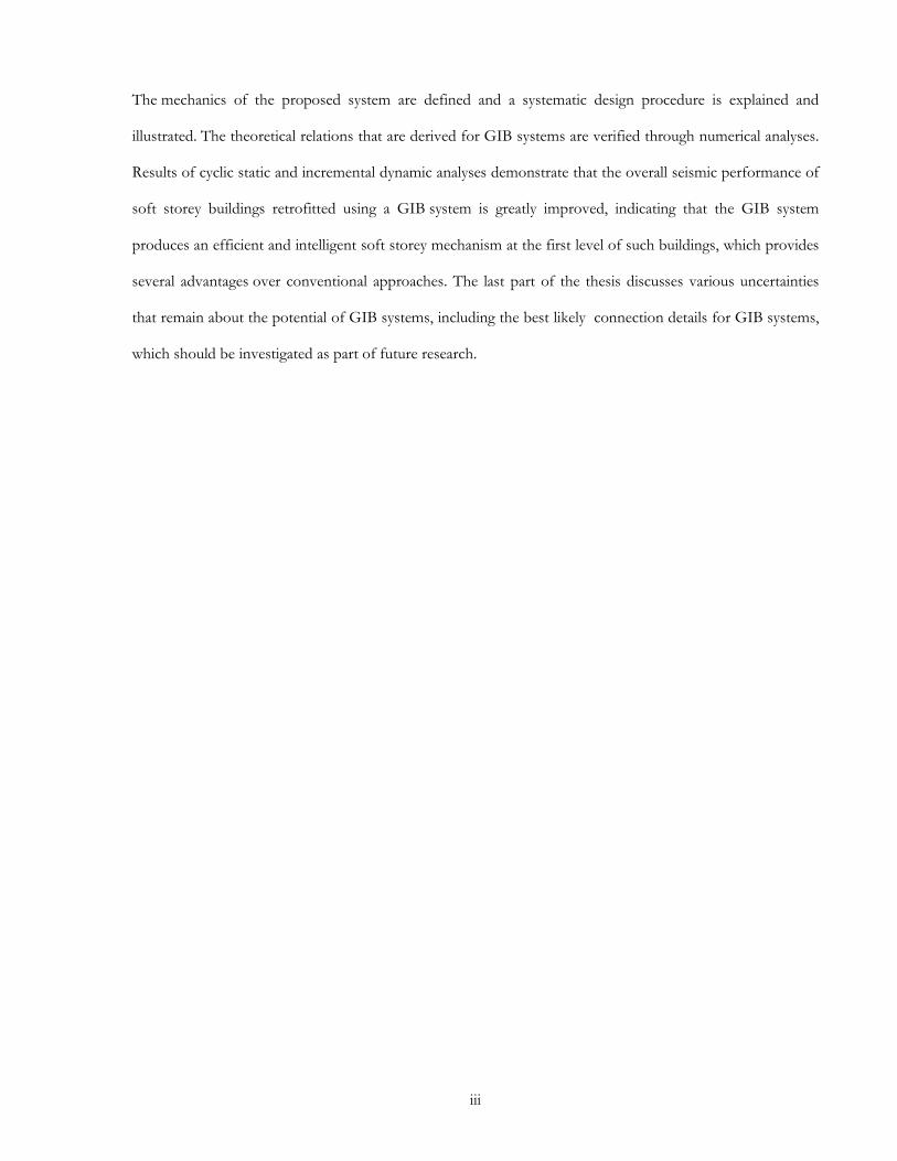
The mechanics of the proposed system are defined and a systematic design procedure is explained and
illustrated. The theoretical relations that are derived for GIB systems are verified through numerical analyses.
Results of cyclic static and incremental dynamic analyses demonstrate that the overall seismic performance of
soft storey buildings retrofitted using a GIB system is greatly improved, indicating that the GIB system
produces an efficient and intelligent soft storey mechanism at the first level of such buildings, which provides
several advantages over conventional approaches. The last part of the thesis discusses various uncertainties
that remain about the potential of GIB systems, including the best likely connection details for GIB systems,
which should be investigated as part of future research.

iv
ACKNOWLEDGEMENTS
First, I would like to express my deepest gratitude to all my supervisors:
• Professor Tim Sullivan, for his invaluable advising in all the time of my research and writing of this
thesis. Without his supervision and constant help, this dissertation would not have been possible.
• Professor Constantin Christopoulos, for his gracious support, excellent guidance and insightful
comments through my thesis. Working under his supervision was a unique instructive experience for
me.
• Professor Gian Michele Calvi, for his support, guidance and encouragement during my research
period. He is definitely one of my respected professors.
I was fortunate to work with such expert supervisors having experiences from different continents. You
kindly shared your wisdom with me and greatly helped me to having a worldwide perspective to problem
solving. Thank you all.
I am grateful to Professor Nigel Priestley for providing his elegant guidance in the beginning of my thesis. His
comments were very helpful to form the general idea of my thesis.
I gratefully acknowledge Professor Guido Magenes and Mr. Mario Galli for providing background data and
analytical models of the case study structure.
In addition to my advisors, I would like to thank the UME School Board in Pavia and the Graduate Student's
Union at the University of Toronto for providing me the opportunity of taking the advantage of the Joint
Placement Program at these two universities.
I would like to thank the financial support offered by the ROSE programme at the UME School, IUSS Pavia
as well as the Italian national 2010-2013 RELUIS project. I would like to thank Professor Christopoulos who
provided me additional funding from the University of Toronto.
I especially thank my mom and dad as well as my brothers Ehsan and Soroosh for all their love over the
years. Without their constant support and encouragement, I would have never given myself the chance to
continue my education.
As an international student, I had the privilege of interacting with wonderful people from different parts of
the world. I want to express my gratitude to all my friends who created one of my best memorable times with
them: Mostafa Masoudi, Fereidon Atarodi, Sevgi Ozcebe, Sujith Mangalathu, David Ruggiero, Paolo Calvi,
Paola Costanza, Fei Tong.

v
Thanks to my class mates Abbas Mirfattah, Guney Ozcebe and Jetson Ronald for their warm messages in the
last days of our theses submission. I would like to also thank all my officemates in GB-403C to provide a
friendly atmosphere during my study at the University of Toronto.
Special thanks to my friend Mohsen Kohrangi, who did an unforgettable job to deliver the hard copy of my
thesis to IUSS Pavia.
Finally, I would like to thank the quite patient and unwavering love of my wife Marjan Haji Heshmati. She
was the only one who was continuously beside me during the last four years of my PhD study. You dedicated
your best part of your lifetime to me. This thesis is dedicated to you.
vi
TABLE OF CONTENTS
ACKNOWLEDGEMENTS ........................................................................................................................................................ iv
TABLE OF CONTENTS ............................................................................................................................................................ vi
LIST OF FIGURES ....................................................................................................................................................................... ix
LIST OF TABLES ........................................................................................................................................................................ xv
LIST OF SYMBOLS.................................................................................................................................................................... xvi
LIST OF ACRONYMS ............................................................................................................................................................... xxi
LIST OF ACRONYM IN CASE STUDIES ......................................................................................................................... xxii
1. INTRODUCTION .................................................................................................................................................................... 1
1.1 MOTIVATION: ....................................................................................................................................................................... 1
1.2 BACKGROUND ...................................................................................................................................................................... 1
1.3 LITERATURE OVERVIEW ..................................................................................................................................................... 3
1.3.1 Modern Architecture and Soft Storeys ................................................................................................................ 3
1.3.2 Earthquake Engineering and Soft Storeys .......................................................................................................... 4
1.4 OBJECTIVE AND SCOPE OF THE THESIS ........................................................................................................................... 4
1.5 ORGANIZATION OF THESIS................................................................................................................................................ 5
2. CLASSIFICATION OF SOFT STOREY BUILDINGS ................................................................................................... 5
2.1 INTRODUCTION .................................................................................................................................................................... 6
2.2 DISCONTINUOUS STRUCTURAL WALLS OR INFILLS ....................................................................................................... 6
2.3 STRONG BEAM – WEAK COLUMN IN FRAME TYPE ....................................................................................................... 8
2.4 DISCONTINUOUS LOAD PATHS ......................................................................................................................................... 9
2.5 STRUCTURAL WALLS WITH LARGE OPENINGS AT THE BASE .................................................................................... 11
2.6 SUMMARY AND CONCLUSION .......................................................................................................................................... 12
3. ASSESSMENT CASE STUDIES .......................................................................................................................................... 13
3.1 INTRODUCTION .................................................................................................................................................................. 13
3.2 DESCRIPTION OF THE CASE STUDY ................................................................................................................................ 13
3.3 MODELLING APPROACH ................................................................................................................................................... 16
3.3.1 Modelling of beams and columns ....................................................................................................................... 16
3.3.2 Modelling of masonry infills: ............................................................................................................................... 20
3.3.3 Modelling of joint elements: ................................................................................................................................ 22
3.4 GROUND MOTION USED FOR TIME HISTORY ANALYSIS........................................................................................... 24
3.5 ANALYTICAL RESULTS ....................................................................................................................................................... 25
3.5.1 Variant 1: Uniform Distribution of Infills (FI) ................................................................................................ 26
3.5.2 Variant 2: Partial Distribution of Infills- Soft First Storey (SS)..................................................................... 30
3.5.3 IDA response comparison of variants ............................................................................................................... 35
3.6 SUMMARY AND CONCLUSION .......................................................................................................................................... 39
4. FACTORS AFFECTING SOFT STOREY RESPONSE ................................................................................................ 41
4.1 INTRODUCTION .................................................................................................................................................................. 41

vii
4.2 EFFECT OF P-DELTA ......................................................................................................................................................... 41
4.2.1 Introduction ............................................................................................................................................................ 41
4.2.2 Effect of P-Delta on hysteretic response .......................................................................................................... 43
4.2.3 Design procedure for P-Delta effects ................................................................................................................ 44
4.2.4 Code recommendations ........................................................................................................................................ 44
4.2.5 Numerical results ................................................................................................................................................... 45
4.2.6 Effect of Increased P-Delta Effects ................................................................................................................... 46
4.3 EFFECT OF POST YIELD STIFFNESS ................................................................................................................................ 48
4.4 EFFECT OF DURATION OF GROUND MOTION ............................................................................................................... 49
4.4.1 Selection of records ............................................................................................................................................... 49
4.4.2 Match records to the design spectra and cornet period 2sec ......................................................................... 50
4.5 KEY CHARACTERISTICS AFFFECTING COLUMN HYSTERETIC BEHAVIOUR ............................................................. 52
4.5.1 Description of RC Column Categories .............................................................................................................. 52
4.5.2 Description of numerical modelling ................................................................................................................... 54
4.5.3 Verification of numerical modelling with an experimental result ................................................................. 55
4.5.4 Numerical results ................................................................................................................................................... 57
4.5.5 Comparison of cyclic analysis with the section analysis ................................................................................. 64
4.5.6 Effect of column characteristics on the demand to capacity ratio ............................................................... 67
4.6 DISCUSSION OF RESULTS ................................................................................................................................................... 69
4.7 SUMMARY AND CONCLUSION .......................................................................................................................................... 71
5. GAPPED INCLINED BRACE SYSTEM TO RETROFIT SOFT STOREY BUILDINGS ................................. 73
5.1 INTRODUCTION .................................................................................................................................................................. 73
5.1 EFFECTIVE AXIAL FORCE TO COUNTERACT P-DELTA EFFECTS .............................................................................. 75
5.2 EFFECT OF AXIAL LOADS ON THE DEFORMATION CAPACITY OF RC COLUMNS ................................................... 77
5.3 effP FOR RC COLUMNS ...................................................................................................................................................... 77
5.3.1 Verification with fibre analysis ............................................................................................................................ 78
5.3.2 Effect of effP on a column response ................................................................................................................. 79
5.4 PROPOSAL OF A GAPPED INCLINED BRACE TO ACHIEVE THE effP ........................................................................ 80
5.5 MECHANICS OF THE GIB SYSTEM .................................................................................................................................. 81
5.5.1 Initial position of the GIB ................................................................................................................................... 81
5.5.2 Gap distance ........................................................................................................................................................... 83
5.5.3 Design of the inclined brace ................................................................................................................................ 84
5.5.4 Design Summary .................................................................................................................................................... 85
5.6 DESIGN EXAMPLE AND NUMERICAL VERIFICATION ................................................................................................. 86
5.7 PARAMETRIC STUDY .......................................................................................................................................................... 88
5.8 NUMERICAL CYCLIC RESPONSE OF A SOFT STOREY FRAME RETROFITTED WITH THE GIB SYSTEM ............... 89
5.9 SUMMARY AND CONCLUSION .......................................................................................................................................... 92
6. SEISMIC RESPONSE OF BUILDINGS USING GIB SYSTEM AND DESIGN RECOMMENDATIONS ......................................................................................................................................... 94

viii
6.1 INTRODUCTION .................................................................................................................................................................. 94
6.2 SOFT STOREY CONCEPT FOR MULTI STOREY BUILDINGS ......................................................................................... 94
6.3 DESIGN CONSIDERATION OF SOFT STOREY BUILDINGS USING THE GIB SYSTEM ............................................. 94
6.4 NUMERICAL INVESTIGATION .......................................................................................................................................... 97
6.5 GIB- 1 VARIANT ................................................................................................................................................................. 98
6.5.1 Numerical Modelling........................................................................................................................................... 100
6.5.2 Verification with Nonlinear Fiber Element modelling ................................................................................. 100
6.5.3 Comparison of variants using fiber analysis ................................................................................................... 105
6.5.4 Results from Nonlinear Time History Analyses ............................................................................................ 106
6.6 COMPARISON OF VARIANTS AT FLOOR LEVEL ............................................................................................................ 110
6.7 COMPARISON OF IDA RESULTS .................................................................................................................................... 112
6.7.1 IDA results............................................................................................................................................................ 112
6.8 EFFECT OF GAP DISTANCE ............................................................................................................................................ 113
6.9 EFFECT OF GIB LOCATIONS: GIB-2 VARIANT AND GIB-3 VARIANT .................................................................... 114
6.9.1 Seismic performance of GIB scenarios ........................................................................................................... 116
6.10 COLLAPSE POTENTIAL OF CASE STUDY VARIANTS ................................................................................................. 117
6.11 SUMMARY AND CONCLUSION ....................................................................................................................................... 117
7. FUTURE STUDIES REGARDING THE UNCERTAINTIES OF THE GIB SYSTEM .................................... 119
7.1 INTRODUCTION ................................................................................................................................................................ 119
7.2 CONSTRUCTABILITY ........................................................................................................................................................ 119
7.3 STRESS CONCENTRATION AT THE CONNECTION ...................................................................................................... 121
7.3.1 Connection of GIB to beam:............................................................................................................................. 121
7.3.2 Connection of GIB to column .......................................................................................................................... 122
7.3.3 Improved Connection of GIB to column ....................................................................................................... 124
7.4 EFFECT OF SUPPLEMENTAL DAMPING ON RESPONSE OF GIB-3 VARIANT ....................................................... 124
7.5 SUMMARY AND CONCLUSION ........................................................................................................................................ 126
8. CONCLUSIONS .................................................................................................................................................................... 128
8.1 CHAPTER 1 AND 2 ............................................................................................................................................................ 128
8.2 CHAPTER 3 ......................................................................................................................................................................... 128
8.3 CHAPTER 4 ......................................................................................................................................................................... 129
8.4 CHAPTER 5 ......................................................................................................................................................................... 129
8.5 CHAPTER 6 ......................................................................................................................................................................... 129
8.6 CHAPTER 7 ......................................................................................................................................................................... 130
REFERENCES ............................................................................................................................................................................ 131

ix
LIST OF FIGURES
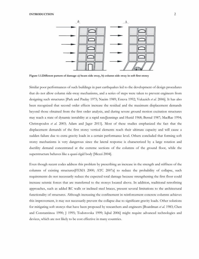
Figure 1.1.Different pattern of damage a) beam side sway, b) column side sway in soft first storey ............................... 2
Figure 1.2.Villa Savoye, the early construction of the open ground storey buildings, picture from
the art of the architect [Filler 2009] ....................................................................................................................... 3
Figure 1.3.Bauhaus Dessau, the open ground storey buildings[Poling 1977] ....................................................................... 4
Figure 2.1.Common residential building with disconnection of stiff elements in the first level ....................................... 7
Figure 2.2.Typical damage due to infill discontinuity, a)Managua, 1972 [NISEE 1972] ,
b)Izmit 1999 [NISEE 1999] ................................................................................................................................... 7
Figure 2.3. Common existing Strong beam – weak column frames ....................................................................................... 8
Figure 2.4. Damage to soft storey behaviour a: Strong beam- weak column in 2010 Haiti
Earthquake ,[NISEE 2010b] b: poor joint connection in the first floor in 1999
Turkey earthquake, [NISEE 2010b], c: lack of confining at thejoint in 1994
Northridge earthquake [Blakeborough 1994] ...................................................................................................... 9
Figure 2.5.Discontinuous load path causes soft storey mechanism ...................................................................................... 10
Figure 2.6.Typical damage due to wall discontinuity a) Olive View hospital, 1971 San Fernando
earthquake [NISEE 2010a] b) Imperial Country Service building, 1979
Imperial Valley earthquake [NISEE 1979] ........................................................................................................ 10
Figure 2.7. Structural wall with opening in the first and typical floors ................................................................................. 11
Figure 2.8. a) Masonry building with large opening at base, Loma Prieta, 1989 b) detail damage to the pier .............. 11
Figure 3.1. Six-storey concrete frame: a) bare frame, b) full infill uniform distribution (FI), c)
Partial infill disconnected in the first floor or Soft storey (SS) ...................................................................... 14
Figure 3.2. Geometric and mechanical properties of beams and columns, from Galli [2006] ....................................... 15
Figure 3.3. Takeda hysteretic rule, Emori unloading [Otani 1974] ....................................................................................... 17
Figure 3.4. Mechanical properties defined for columns a) Moment-Curvature, b) axial load–moment interaction .... 18
Figure 3.5. Shear capacity of columns at the first floor .......................................................................................................... 19
Figure 3.6. Hysteretic cycles of Masonry struts, [Carr 2004] .................................................................................................. 22
Figure 3.7. Modelling of beam column joint [Trowland 2003] .............................................................................................. 22
x
Figure 3.8. Monotonic and cyclic behaviour of shear hinge joint model, [Pampanin et al. 2002] .................................. 23
Figure 3.9. Pampanin Hysteretic rule used in Ruaumoko, [Carr 2004] ................................................................................ 24
Figure 3.10. Acceleration and displacement Response Spectra for the selected records sets ......................................... 26
Figure 3.11. Peak floor acceleration profile obtained from the nonlinear time-history
analysis for different hazard levels, full infill (FI) variant ................................................................................ 27
Figure 3.12. Inter storey drift profile obtained from nonlinear time-history analysis for
different hazard levels, full infill (FI) variant .................................................................................................... 28
Figure 3.13. Inter storey residual drift profile obtained from nonlinear time-history analysis
for different hazard levels, full infill (FI) variant ............................................................................................. 29
Figure 3.14. Peak response of interests obtained from incremental dynamic analysis,
full infill (FI) variant ............................................................................................................................................... 30
Figure 3.15. Peak floor acceleration profile obtained from nonlinear time-history analysis
for different hazard levels, Soft storey (SS) variant .......................................................................................... 31
Figure 3.16. Inter storey drift profile obtained from nonlinear time-history analysis for
different hazard levels, soft storey (SS) variant ................................................................................................. 32
Figure 3.17. Residual storey drift profile obtained from nonlinear time-history analysis for
different hazard levels, soft storey (SS) variant ................................................................................................. 33
Figure 3.18. Peak response of interests obtained from incremental dynamic analysis,
soft storey (SS) variant ........................................................................................................................................... 34
Figure 3.19. Displacement damage index (DDI) for beams and columns obtained from
nonlinear time-history analysis for different hazard levels, soft storey (SS) variant ................................... 35
Figure 3.20. Comparison of the peak inter storey drift ratio (PRD) obtained
from IDA for two variants of FI and SS ........................................................................................................... 36
Figure 3.21. Comparison of the residual inter storey drift ratio (RRD) obtained from IDA
for two variants of full infill (FI) and partial infill (SS) ................................................................................... 37
Figure 3.22. Comparison of the average inter storey drift ratio obtained from IDA for
two variants of full and partial infill .................................................................................................................... 37
Figure 3.23. Comparison of the peak floor acceleration (PFA) obtained from IDA for
two variants of full and partial infill .................................................................................................................... 38
Figure 3.24. Mean acceleration spectra for a period between 0.3 and 2.1 sec .................................................................... 38

xi
Figure 3.25. Comparison of the beams and columns DDI for the two FI and SS variants ............................................. 39
Figure 4.1. P-∆ Effects on design moments ............................................................................................................................ 42
Figure 4.2. P-∆ Effects on force and response characteristics: a) general load deformation relationship;
b) bilinear positive curve ....................................................................................................................................... 42
Figure 4.3. Comparison of IDA response with and without P-∆ effects: a) peak drift ratio, b) residual drift ratio .. 46
Figure 4.4. Dummy column modelling for considering effect of axial load........................................................................ 47
Figure 4.5. Comparison of responses obtained from incremental NTHA when the total gravity load is doubled ..... 47
Figure 4.6. Effect of post yield ratio of responses .................................................................................................................. 48
Figure 4.7. Acceleration and displacement Response Spectra for the selected records sets:
matched to the displacement spectrum soil C, Td=8.sec ............................................................................... 51
Figure 4.8. Acceleration and displacement response spectra match to displacement spectra for
soil A with corner period of 2sec soil type A: a) Short duration records b) Long duration records ....... 51
Figure 4.9. Comparison responses for short and long duration records ............................................................................ 52
Figure 4.10. Different configuration of steel reinforcement and column size of the RC concrete columns ............... 54
Figure 4.11. Geometrical characteristics of the specimen and history of cyclic loading .................................................. 56
Figure 4.12. Comparison between numerical and experimental results of cyclic behaviour of RC column ................ 57
Figure 4.13. Effect of longitudinal reinforcement ratio on column hysteretic response (Moment-chord rotation)
Variant I, D=0.4, σ� = 0.3 confinement factor: 1.2, cantilever length =3m ............................................. 58
Figure 4.14. Effect of column dimension on hysteretic response (Moment-Chord rotation)
Variant II, ρ=0.015, σ� = 0.3 confinement factor: 1.2, cantilever length =3m ........................................ 60
Figure 4.15. Effect of axial force ratio (σ�)on column hysteretic response (Moment-Chord rotation),
Variant III: Column dimension: 40x40cm, ρ=0.015, confinement factor: 1.2, cantilever length =3m .. 61
Figure 4.16. Effect of confinement factor on column hysteretic response (Moment-Chord rotation)
Variant IV: Column dimension: 40x40cm, ρ=0.015 σ� = 0.3 , cantilever length =3m......................... 62
Figure 4.17. Comparison of key characteristics on the cyclic behaviour of RC columns ................................................ 63
Figure 4.18. Effect of key characteristics on the hysteretic response of RC columns ..................................................... 63
Figure 4.19. Section stress – strain distribution in reinforcement concrete column ........................................................ 65
Figure 4.20. Comparison of key characteristics on column response based on section analysis ................................... 66
xii
Figure 4.21. Comparison of key characteristics on Demand-Capacity Ratio (DCR) ....................................................... 68
Figure 4.22. Possible means of de-coupling gravidity loads from lateral loads in a soft storey building ...................... 71
Figure 5.1. Proposed mitigation strategies, a) roller system b) gapped inclined braced (GIB) system ........................ 74
Figure 5.2. Single-Degree-of-freedom system subject to axial load and lateral displacement......................................... 75
Figure 5.3 a) Influence of the P-Delta effect and the effP on the force-displacement response
b) Effective axial force ( effP ) ............................................................................................................................... 76
Figure 5.4.a Numerical analysis of a 0.40m×0.40m RC column: 1.5%ρ = , 1.15CF = , axial load ratio
range 0: 0.05 to 0.5 in increments of 0.05 a) Axial load ratio versus lateral drift capacity ratio,
( effP in normalized form), b) Lateral resistance versus lateral drift capacity ratio, referred to
as degraded capacity curve ................................................................................................................................... 78
Figure 5.5. Gapped-Inclined Brace (GIB) system to the existing column a) Initial condition
b) Closing gap condition c) Ultimate condition ................................................................................................ 80
Figure 5.6. Mechanics of the GIB system a) Initial position, b) elastic behaviour of the column before gap is
closed c) post yield condition ............................................................................................................................... 81
Figure 5.7. Effect of the GIB on the lateral resistance and the displacement capacity of RC columns ....................... 82
Figure 5.8. Axial force in the column and the inclined brace ............................................................................................... 87
Figure 5.9. Total behaviour of the proposed method in comparison to the existing column only ............................... 87
Figure 5.10. Effect of the GIB system on response of 0.40x0.40m RC columns with different height H .................. 88
Figure 5.11. Effect of the GIB system on response of 0.40x0.40m RC columns with different
height initial axial load ratio ................................................................................................................................. 89
Figure 5.12. Effect of the GIB system on response of 0.40x0.40m RC columns with different
height initial confinement actor CF .................................................................................................................... 89
Figure 5.13. Single one storey RC frame retrofitted using GIB and subjected to quasi-static loading ......................... 90
Figure 5.14. Axial force history of the right and left gap elements, b) Moment –
Curvature response of the existing column ....................................................................................................... 91
Figure 5.15. Moment – Curvature response of the existing column ................................................................................... 92
Figure 5.16. Hysteretic response of the hybrid system in comparison to the existing frame........................................... 92
Figure 6.1. Case study building configuration (details in chapter 3) .................................................................................... 97

xiii
Figure 6.2. Position of the GIB system in the soft storey building bases on three configurations:
a) GIB 1 variant, b) GIB 2 variant, c) GIB 3 variant ...................................................................................... 99
Figure 6.3. Modelling of GIB system in Ruaumoko for time history analysis ................................................................. 100
Figure 6.4. Modelling masonry infills in Ruaumoko, a) infill panel element configuration
b) shear spring modelling .................................................................................................................................... 102
Figure 6.5. Comparison of the pushover curves obtained from the lumped plasticity and the fibre
element modelling of the existing soft storey frame ...................................................................................... 103
Figure 6.6. modelling of GIB system in Seismo-Struct for push over analysis ............................................................... 103
Figure 6.7. Axial forces in the first storey columns and the GIB of the GIB-1 variant: comparison
between fibre models and lumped plasticity models, see Figure 6.2........................................................... 104
Figure 6.8. Push over curve capacity of the GIB-1 variant from nonlinear fibre element (SeismoStruct)
modelling and lumped plasticity modelling(Ruaumoko) ............................................................................... 105
Figure 6.9. Push over curve capacity for the six-storey frame buildings a) Full infill, b) Partial infill,
c) GIB-1 variant ................................................................................................................................................... 106
Figure 6.10. Damage limit state pattern in the six-storey frame a) Full infill, b) Partial infill, c GIB-1 variant,
(Dr : Roof drift(%) ; Vb: Base shear (kN)) ........................................................................................................ 107
Figure 6.11. Global seismic response in GIB-1 variant obtained from NTHA for three earthquakes:
a) Global hysteresis, b) Inter-storey drift, c)Floor acceleration ................................................................... 108
Figure 6.12. Element hysteretic responses in GIB-1 variant: a) Moment-curvature of exterior Beams
and columns, b) Moment-curvature of interior Beams and columns c) Axial GIBs hysteresis ............. 109
Figure 6.13. Axial force on the columns and the GIBs of the first storey, GIB-1 variant ............................................. 110
Figure 6.14. Response parameters at storey levels ................................................................................................................. 111
Figure 6.15. IDA responses ....................................................................................................................................................... 112
Figure 6.16. Effect of gap distance on the seismic response of the GIB-1 variant ......................................................... 114
Figure 6.17. Locations of GIBs ................................................................................................................................................ 115
Figure 6.18. Seismic parameters for different GIB scenarios a) DDI, b) Peak floor acceleration ................................ 116
Figure 6.19. Seismic parameters for different GIB scenarios a) DDI, b) Peak floor acceleration ................................ 117
Figure 7.1. Hysteretic response of the hybrid system using different behaviour of the inclined column.................... 120
xiv
Figure 7.2. A proposed connection for the GIB system using the offset ........................................................................ 121
Figure 7.3. a)Possibility of Shear failure at the beam and the GIB connection, b) possible retrofit strategy ............ 122
Figure 7.4. Connection of the GIB system to the column only: a) connection detail,
b) actions in the gusset plate, c) actions in the bolts ...................................................................................... 123
Figure 7.5. Alternative connection proposal of GIB to column using gusset plate........................................................ 124
Figure 7.6. Adding viscose dampers to the GIB-3 variant in the numerical modelling (DGIB-3 variant) ................. 125
Figure 7.7. Effect of adding dampers on the response of the GIB-3 variant ................................................................... 126

xv
LIST OF TABLES
Table 3.1. Masonry mechanical properties ................................................................................................................................ 19
Table 3.2. Parameters of the equivalent diagonal strut model [Bertoldi 1993] ................................................................... 20
Table 3.3. Masonry mechanical properties ................................................................................................................................ 21
Table 3.4. Failure modes in masonry infill panels [Bertoldi 1993] ........................................................................................ 21
Table 3.5. Record Set used for nonlinear time history analysis ............................................................................................. 25
Table 3.6. Summary of response parameters obtained for three variants of case 1 with full infill,
partial infill and bare frame ................................................................................................................................... 35
Table 4.1. Long duration record sets .......................................................................................................................................... 50
Table 4.2. Characteristics of different column studied, with a cantilever length of 3m .................................................... 53
Table 6.1. Column configurations at the open ground level ................................................................................................. 98
Table 6.2. GIB configurations associated to each column type for GIB-1 ........................................................................ 99
Table 6.3. GIB configurations for different scenarios ......................................................................................................... 115
Table 7.1. Shear force in beams at the first floor of the GIB-1 building .......................................................................... 122
xvi
LIST OF SYMBOLS
α Takeda parameter
Ac Column cross section
Ag Gross section area of RC column
αP∆ Second order amplification factor
Asi Total are of longitudinal reinforcement at layer i in section analysis
Ast Total area of longitudinal reinforcement
b Width of RC column section
β Takeda parameter, Strength reduction factor
βP∆ Second order parameter
bw Equivalent height of infill strut
CF Confinement factor
∆ displacement
db beam depth in joint modelling
∆ci Displacement capacity at level i
DCR Demand-capacity ratio
∆d Demand displacement
∆d Equivalent target displacement of building
∆f Lateral displacement of first floor
∆gap Gap distance inside GIB system
∆GIB Distance between the base of GIB system and the bace of RC column
∆Lc Axial elongation of RC column
dm Ultimate displacement
∆u Roof lateral displacement at ultimate state

xvii
dw Diagonal length of infill panel
dy Yield displacement
∆y Yield drift displacement
ε Axial strain of the GIB system, non dimensional mass properties
Ec Elastic modulus of concrete
Gc Shear modulus of concrete
εc Extreme concrete fibre compression strain
εcu Ultimate concrete strain
ED Energy dissipated per cycle at target displacement
Es Young'g modulus of steel
εsn Reinforcement strain at maximum distance from the neutral axis
Ew Elastic modulus of masonry infill
εy Yield axial strain of GIB system
Fy Yield force in Takeda hysteretic rule
F0 Lateral force at yield without P-Delta effects
f'c Compressive strength of concrete
fc(x) Force in concrete in section x
f'cc Confined concrete compressive strength
Fi Lateral force at level i
Fp Lateral force at yield with P-Delta effects
Fw Horizontal projection of ultimate load of masonry infill
f'w Compressive resistance of material of masonry infill
fws Shear resistance of masonry infill under diagonal compression
fwu Sliding resistance of mortar joints of masonry infill
Fyh Yield strength of transverse reinforcement in RC column
fys Rebar yield strength

xviii
γ non dimensional frequency properties
H Inter-storey height
Hc Column cantilever height
Hi Height of building at storey i
hw Height of infill panel
Ip Moment of inertial of column section
ϕ curvature in section analysis
ϕy Yield curvature
K0 First order initial stiffness
K1 Parameter of the equivalent diagonal strut model
K2 Parameter of the equivalent diagonal strut model
Kc Axial stiffness of RC column
Keff Effective stiffness
Ker Equivalent stiffness of the storeys above the first floor
Kf First floor stiffness
kp Second order initial stiffness
Ku Unloading stiffness
λ Parameter of the equivalent diagonal strut model
L half of joint panel height in joint modelling
Lb0 Length of GIB system at closing gap
LGIB Initial length of GIB system
Lp Plastic hinge length of RC column
M Bending moment at the base of cantilever
M Mass
µ ductility
Mi Moment at level i

xix
µm Limit of ductility for P-Delta effects
ng Number of values in geometric mean
P Gravity load
P0 Axial load on RC columns in parametric study
Pb Axial force in GIB system
Pu Axial load on column at the ultimate sate
θ Panel inclination respect to horizontal
θ Inter-storey drift ratio
θGIB Initial angle of GIB system
θi Drift Capacity at level i
θP∆ Stability index
θy Yield lateral drift ratio of
ρ Reinforcement ratio
R Ratio of upper floor storeys stiffness to that of first floor
r , r0 First order post yield stiffness ratio
Rd Spectral displacement reduction factor
rp Second order post yield stiffness ratio
ρsx Geometrical ratio of confining reinforcement in horizontal direction
ρsy Geometrical ratio of confining reinforcement in vertical direction
ρv Geometrical ratio of confining reinforcement
σ0 Initial axial load ratio
σdes Inclined brace design stress
σv Vertical compression stress on masonry infill due to gravity loads
σw Equivalent strength of masonry infill
τ Ratio of total vertical load (dead load plus reduced live load) to dead load

xx
Teff Effective Period
tw Thickness of infill panel
VBc Base shear capacity of first floor
VBd Demand base shear
Vu,col Lateral strength of RC column at ultimate state
Vy,col Lateral strength of RC column at yield
ωer Natural frequency of storeys above the first floor
ωf Natural frequency of first floor
ξeq Equivalent damping ratio
xg Geometric mean value of response
xxi
LIST OF ACRONYMS
FMPM first mode participation mass in the elastic range
GIB Gapped Inclined Brace
IDA Incremental Dynamic Analysis
PDR Peak Inter-Storey Drift Ratio
PFA Peak Floor Acceleration
PRDR Peak Inter-Storey Residual Drift Ratio
DBE Design basis Earthquake
FE Frequent Earthquake
MCE Maximum Credible Earthquake

xxii
LIST OF ACRONYM IN CASE STUDIES
Variant Acronym Description
1 FI-NPD Full Infill No P-Delta
2 SS-NPD Soft Storey No P-Delta
3 BF-NPD Bare Frame No P-Delta
4 FI Full Infill with P-Delta
5 SS Soft Storey with P-Delta
6 BF Bare Frame with P-Delta
7 SS-DPD Similar to SS when P-Delta effects are doubled
8 SS-R-0.05 Similar to SS with Post yield stiffness ratio R=0.025
9 SS-R-0.025 Similar to SS with Post yield stiffness ratio R=0.05
10 SS-R-0.10 Similar to SS with Post yield stiffness ratio R=0.10
11 SS-R-0.15 Similar to SS with Post yield stiffness ratio R=0.15
12 GIB-I SS retrofitted Using GIB system- Configuration I
13 GIB-II SS retrofitted Using GIB system- Configuration II
14 GIB-III SS retrofitted Using GIB system- Configuration III
15 DGIB-25 Similar to GIB-III with Supplemental damping C=25 kN.s/m
16 DGIB-50 Similar to GIB-III with Supplemental damping C=50 kN.s/m
17 DGIB-150 Similar to GIB-III with Supplemental damping C=150 kN.s/m
18 DGIB-250 Similar to GIB-III with Supplemental damping C=250 kN.s/m

1
1.INTRODUCTION
1.1 MOTIVATION:
Over the past few centuries, the number of buildings constructed in urban areas have increased saliently. The
urban zoning regulations in many countries encourage engineers and architects to consider modern
architectural configurations in their designs. Open ground storey buildings (also known as soft storey, pilotis
or soft, weak or open front, SWOF) are one of the most common types of such configurations. For example,
an extensive study by the Applied Technology Council [ATC-52-3 2009] indicated that in San Francisco, 2800
out of 4600 residential wood frame buildings had significant openings at the ground level. Having parking,
retail areas, storefront windows, shopping areas, and lobbies at the first floor of multi storey buildings are the
architectural and social advantages of such buildings. Similar statistics have been reported for other
communities, which indicate the prevalence of such buildings.
On the other hand, earthquake surveys have shown that soft storey buildings are some of the most vulnerable
structures, and their behaviour has been recognized as one of the most undesirable mechanisms by the
structural and earthquake engineering community [Chopra et al. 1973; Rutenberg et al. 1982; Arnold 1984].
Almost two thirds of the 46,000 units that were uninhabitable after the Northridge earthquake and a high
percentage of the death toll were attributed to such buildings [Comerio 1995]. Because of the similarity in
housing stocks, a similar percentage could also be expected for other megacities in the world following a
major earthquake.
Since earthquakes have been recorded, over 8.5 million deaths and almost $2.1 trillion damages have been
reported all around the world [Daniell et al. 2011]. Recently, global fatalities from earthquakes has been
estimated as 100,000 per year [Bilham 2004; USGS 2013]. Considering the high contribution of soft storey
buildings in the loss of life and money, it could be estimated that such buildings were responsible for a few
million fatalities and several billions of dollars of losses.
1.2 BACKGROUND
Beside the architectural advantages, the potential structural benefits of soft storey buildings had also been
studied by well-known researchers as early as the 1930s [Martel 1929; Green 1935; Jacobsen 1938; Chopra et
al. 1973; Arnold 1984].This proposal relied on mitigating the total inertial forces using the soft link concept at
the first floor (Figure 1.1). A number of buildings were designed based on this idea by some engineers and
experts. The six-storey cast-in-place Olive View hospital was a good example of implementing such designs
in the 1970s. However, the building suffered significant damage and it was decided to demolish and rebuilt it
[Mahin et al. 1976a].
INTRODUCTION 2
Figure 1.1.Different pattern of damage a) beam side sway, b) column side sway in soft first storey
Similar poor performances of such buildings in past earthquakes led to the development of design procedures
that do not allow column side-sway mechanisms, and a series of steps were taken to prevent engineers from
designing such structures [Park and Paulay 1975; Naeim 1989; Esteva 1992; Vukazich et al. 2006]. It has also
been recognized that second order effects increase the residual and the maximum displacement demands
beyond those obtained from the first order analysis, and during severe ground motion excitation structures
may reach a state of dynamic instability at a rapid rate[Jennings and Husid 1968; Bernal 1987; MacRae 1994;
Christopoulos et al. 2003; Adam and Jager 2011]. Most of these studies emphasized the fact that the
displacement demands of the first storey vertical elements reach their ultimate capacity and will cause a
sudden failure due to extra gravity loads in a certain performance level. Others concluded that forming soft
storey mechanisms is very dangerous since the lateral response is characterized by a large rotation and
ductility demand concentrated at the extreme sections of the columns of the ground floor, while the
superstructure behaves like a quasi-rigid body [Mezzi 2004].
Even though recent codes address this problem by prescribing an increase in the strength and stiffness of the
columns of existing structures[FEMA 2000; ATC 2007a] to reduce the probability of collapse, such
requirements do not necessarily reduce the expected total damage because strengthening the first floor could
increase seismic forces that are transferred to the storeys located above. In addition, traditional retrofitting
approaches, such as added RC walls or inclined steel braces, present several limitations to the architectural
functionality of structures. Although increasing the confinement in reinforcement concrete columns achieves
this improvement, it may not necessarily prevent the collapse due to significant gravity loads. Other solutions
for mitigating soft storeys that have been proposed by researchers and engineers [Boardman et al. 1983; Chen
and Constantinou 1990; J 1995; Todorovska 1999; Iqbal 2006] might require advanced technologies and
devices, which are not likely to be cost effective in many countries.

INTRODUCTION 3
1.3 LITERATURE OVERVIEW
As mentioned in the previous sections, a series of problems associated with soft storey buildings have ruled
them out in seismic regions. Thus, it is difficult to find much material in the recent literature that implements
the soft storey concept as a reliable tool for retrofitting. To achieve the goal of this thesis, any relevant
literature review is directed inside each chapter separately. However, the following two subsections review
current considerations for soft storey buildings from two different perspectives.
1.3.1 Modern Architecture and Soft Storeys
The first appearance of modern soft storey buildings dates back to 1914, where the famous architect Le
Corbusier developed the term "Dom-ino system" for economic housing [Glassman 2001]. This model, which
was proposed by a pioneer of modern architecture, proposed five points, in which one main point was that
that upper storey slabs should be supported by an open floor plan consisting of perimeter slender columns,
known as pilotis (Floating concept).
Figure 1.2 shows an example of an early open ground storey construction. This concept was followed by
another architect in 1925, Walter Gropius, who proposed Bauhaus buildings, an open ground storey building
using a number of windows on the façade. Figure 1.3 shows a model of a school designed using this idea,
where the building has both horizontal and vertical irregularity. The Bauhaus had a major impact on art and
architecture trends in Western Europe and the North America[Poling 1977].
The two aforementioned concepts became the principal of the modern architecture in the 20th and the 21th
centuries, and spread out quickly all around the world. The open ground floors are nowadays used for socio-
economical purposes including parking, garage space or stores.
The current urban zoning regulations of many countries encourage owners to use soft storey configurations
because the area enclosed by a soft storey is rewarded to them. This area is neither computable as part of the
maximum allowable built area, nor for tax, but is computable for selling purposes [Guevara-Perez 2010].
Figure 1.2. Villa Savoye, the early construction of the open ground storey buildings, picture from the art of the architect
[Filler 2009]

INTRODUCTION 4
Figure 1.3. Bauhaus Dessau, the open ground storey buildings[Poling 1977]
1.3.2 Earthquake Engineering and Soft Storeys
In terms of earthquake engineering, the viewpoint on soft storey buildings is extremely different to that of the
architectural viewpoint. The general recognition is to say that a soft-storey building is one in which
deformations are expected to be concentrated in a single “soft” storey [Bertero 1984]. Based on the current
code definition [FEMA310 1998; UBC 2009], buildings are classified as having a "soft storey" if that level is
less than 70% as stiff as the floor immediately above it, or less than 80% as stiff as the average stiffness of the
three floors above it.
Such buildings are categorised as vulnerable structures to collapse in moderate to severe earthquakes in a
phenomenon known as a soft storey collapse. The weak storey is relatively less resistant than surrounding
floors to lateral earthquake motion, so a disproportionate amount of the building's overall side-to-side drift is
focused on that floor. Subject to such large deformations, the floor becomes a weak point that may suffer
structural damage or complete failure, which could increase the possibility of the collapse of the entire
building. The behaviour of such buildings in recent earthquakes is reviewed in more detail in chapter 2.
1.4 OBJECTIVE AND SCOPE OF THE THESIS
With previous efforts in mind, the main objective of this research is to find a retrofitting strategy for soft
storey buildings that takes advantages of such buildings while mitigating the negative aspects.
Some other potential advantages of soft storey buildings are:
• Limited direct losses: The vast majority of the first floor application are parking or stores. This areas are
less valuable compared to the more expensive part of the building, including residential or office sections.
Thus, by accumulating damage in this "cheap floor", the total repair cost could be minimized.

INTRODUCTION 5
• Indirect loss: The down time could be minimised because only one floor could go out of service, while
the rest of the building could be even at the immediate occupancy performance level. This benefit is
likely to require that some other form of access be provided to upper floors.
• Retrofit cost: Only one floor is required to be retrofitted, which is likely to save cost and time.
1.5 ORGANIZATION OF THESIS
Chapter 2 starts with a brief literature review on the response of buildings with soft storey configurations to
past earthquakes. The common types of such buildings are classified and their seismic responses are
qualitatively reviewed. This chapter indicates that buildings in which masonry infills are disconnected in the
first level are one of the most common types of soft storey building. This conclusion led to the choice of the
building that is extensively studied in Chapter 3.
The seismic vulnerability of a six-storey RC frame building typical of construction practice from the 1970’s is
examined in Chapter 3, initially considering two different infill configurations; the first considers full masonry
infill and the second considers an open ground storey with full masonry infill on all floors except for the first
floor. The seismic response of the two configurations is compared using incremental nonlinear time history
analyses.
To provide insight into the factors affecting the vulnerability of soft storey structures, chapter 4 investigates
the impact of some key characteristics on the soft storey response. The impact of P-Delta effects, the post-yield
stiffness ratio and the ground motion duration on the seismic behaviour of such structures is studied. Then, the
effect of some key characteristics on the cyclic behaviour of columns is numerically investigated. The results
presented in this chapter lead to the definition of a new retrofit approach for soft storey buildings.
Chapter 5 proposes the Gapped-Inclined Brace (GIB) system for retrofitting the seismic response of soft
storey structures that, in addition to reducing the likelihood of collapse at the first level of soft storey
buildings, concentrates seismic damage at this single level, while protecting the rest of the structure located
above. The mechanics of the proposed system are first defined. Theoretical relations and numerical models
are derived to verify the response. The cyclic behaviour of a single degree of freedom RC frame retrofitted
using the GIB system is numerically investigated.
Chapter 6 investigates the dynamic characteristics of MDOF buildings that are retrofitted using the GIB at
the ground floor. This chapter presents a case study of the soft storey building that is retrofitted using the
GIB system. To investigate the effectiveness of alternate retrofit configurations, different scenarios of the
GIB systems is explored.
Chapter 7 highlights uncertainties regarding the performance of the GIB system on the soft storey response,
and recommends future studies to further develop this concept.
6
2.CLASSIFICATION OF SOFT STOREY BUILDINGS
2.1 INTRODUCTION
This chapter presents a brief literature review of the seismic behaviour of buildings using soft storey
configurations in past earthquakes. The common types of such buildings are classified and their seismic
responses are qualitatively reviewed. The result of this chapter lead to the selection of a sample structure that
will be analytically studied in the next chapter.
Soft storey buildings have been classified in four categories [Arnold 1984]: tall first storey, discontinuous
infills, discontinuous shear walls and discourteous load path. A similar classification but with a slightly
broader range is reviewed in this chapter:
• Discontinuous structural walls or infills
• Strong beam - weak column in frame type
• Discontinuous load path
• Walls in large openings at the base
In the following sections, all types of aforementioned structures are discussed.
2.2 DISCONTINUOUS STRUCTURAL WALLS OR INFILLS
These types of structures are often observed in commercial and residential buildings. In such configurations,
masonry partitions or structural walls are disconnected in the first stories due to operational reasons. Vertical
loads are usually transferred by transfer beams and carried by columns to form the lateral load path. In
commercial buildings, this discontinuity is more likely due to the presence of large store-front windows for
business purposes.
Discontinuous infills are the most common type of existing soft storey buildings. In residential buildings, they
are usually present because of large open areas such as parking or garages, which create a first floor that has
fewer walls, and thus, is much softer than the levels above. A comprehensive study on the multifamily
dwelling MFD buildings in Santa Clara County [Selvaduray et al. 2003; Vukazich et al. 2006] indicated that 36
percent of the existing buildings encompassed this architectural configuration, known as the "tuck under
parking". Another study in Berkeley [Bonowitz 2005; MacQuarrie 2005] showed that only 15% of soft storey
buildings had residential use in the ground floor; most of them had non-residential use such as parking or
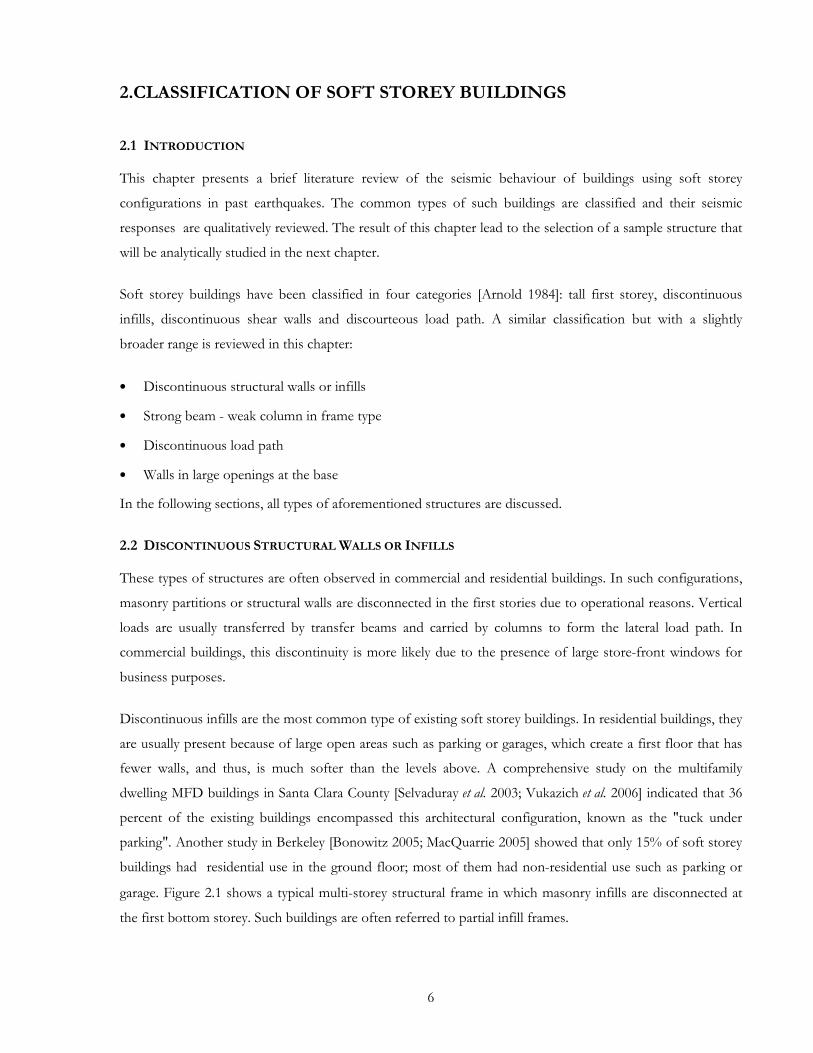
garage. Figure 2.1 shows a typical multi-storey structural frame in which masonry infills are disconnected at
the first bottom storey. Such buildings are often referred to partial infill frames.

CLASSIFICATION OF SOFT STOREY BUILDINGS 7
Figure 2.1. Common residential building with disconnection of stiff elements in the first level
Figure 2.2 shows typical damages to buildings with this type of soft storey configuration during past
earthquakes. On the left side of the figure, there is a two storey RC commercial building "Casa Micasa S.A.",
which suffered significant lateral displacement at the ground floor level during the 1972 Managua Earthquake.
This storey was completely open (except for glass partitions all around), while the upper storey had walls and
partitions that significantly increased the lateral stiffness of this second storey relative to the first. The flexural
plastic hinges formed at the top and bottom of the first storey columns [Bertero 1997]. In the right hand of
this figure, a six-storey residential reinforced concrete building that was damaged in the Izmit, Turkey
earthquake in 1999 is shown. The significant density of masonry infills in the upper storeys omitted in the
first two stories. These floors were completely collapsed, while even windows in the upper stories remained
intact.
a) b)
Figure 2.2. Typical damage due to infill discontinuity, a)Managua, 1972 [NISEE 1972] , b)Izmit 1999 [NISEE 1999]
CLASSIFICATION OF SOFT STOREY BUILDINGS 8
Arnold [1984] stated that if pre-cast cladding systems or lightweight partitions are used in the storeys above
the ground level, the problem might be less significant. Because their in-plane stiffness is not considerable,
especially when their connection to the main structure is poor or they are applied separately.
2.3 STRONG BEAM – WEAK COLUMN IN FRAME TYPE
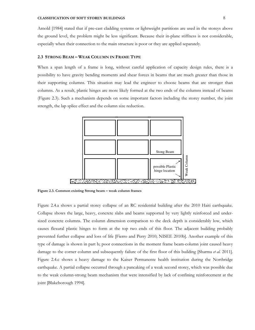
When a span length of a frame is long, without careful application of capacity design rules, there is a
possibility to have gravity bending moments and shear forces in beams that are much greater than those in
their supporting columns. This situation may lead the engineer to choose beams that are stronger than
columns. As a result, plastic hinges are more likely formed at the two ends of the columns instead of beams
(Figure 2.3). Such a mechanism depends on some important factors including the storey number, the joint
strength, the lap splice effect and the column size reduction.
Figure 2.3. Common existing Strong beam – weak column frames
Figure 2.4.a shows a partial storey collapse of an RC residential building after the 2010 Haiti earthquake.
Collapse shows the large, heavy, concrete slabs and beams supported by very lightly reinforced and under-
sized concrete columns. The column dimension comparison to the deck depth is considerably low, which
causes flexural plastic hinges to form at the top two ends of this floor. The adjacent building probably
prevented further collapse and loss of life [Fierro and Perry 2010; NISEE 2010b]. Another example of this
type of damage is shown in part b; poor connections in the moment frame beam-column joint caused heavy
damage to the corner column and subsequently failure of the first floor of this building [Sharma et al. 2011].
Figure 2.4.c shows a heavy damage to the Kaiser Permanente health institution during the Northridge
earthquake. A partial collapse occurred through a pancaking of a weak second storey, which was possible due
to the weak column-strong beam mechanism that were intensified by lack of confining reinforcement at the
joint [Blakeborough 1994].
Stong Beam
Wea
k C
olu
mn
possible Plastic
hinge location

CLASSIFICATION OF SOFT STOREY BUILDINGS 9
(a) (b)
(c)
Figure 2.4. Damage to soft storey behaviour a: Strong beam- weak column in 2010 Haiti Earthquake ,[NISEE 2010b] b:
poor joint connection in the first floor in 1999 Turkey earthquake, [NISEE 2010b], c: lack of confining at the
joint in 1994 Northridge earthquake [Blakeborough 1994]
2.4 DISCONTINUOUS LOAD PATHS
Discontinuous load paths are to some extent similar to the first group, in which shear walls or braces are
disconnected at the top of the first level (Figure 2.5). The use of large entrances including lobbies or business
shops are the common reasons of such configurations. Figure 2.5.a shows a situation that the shear force at
the second storey is transferred through the first floor diaphragm to other resisting elements below. If the
diaphragm cannot transfer all shear forces from the stiffer span to the adjacent one, it could cause a soft
storey mechanism at the first floor. The concern is that the wall or braced frame may have more shear
capacity than considered in the design. These capacities impose overturning forces that could overwhelm the
columns. While the strut or connecting diaphragm may be adequate to transfer the shear forces to adjacent
elements, the columns which support vertical loads are the most critical [FEMA310].

CLASSIFICATION OF SOFT STOREY BUILDINGS 10
(a) (b)
Figure 2.5. Discontinuous load path causes soft storey mechanism
Discontinuous load paths can also occur due to the omission of structural walls in some part of the structural
system (Figure 2.5b). Olive View Hospital is a well-known example of a discontinuous structural wall as
shown in Figure 2.6.a. This lateral load resisting structural system did not extend through the first and ground
floors of the structure, so that the slabs and columns of these lower two stories behaved more like a flexible,
moment resisting space frame.
(a) (b)
Figure 2.6. Typical damage due to wall discontinuity a) Olive View hospital, 1971 San Fernando earthquake [NISEE 2010a]
b) Imperial Country Service building, 1979 Imperial Valley earthquake [NISEE 1979]
Event though the building was designed for lateral forces higher than code requirements, the building had
been badly damaged (75 cm residual deformation at the ground floor) during the 1971 San Fernando
earthquake and subsequently had to be demolished. An analytical study by Mahin et al. [1976b] confirmed that
the brittle shear failure at the ground floor columns and the near field characteristic of the ground motion
were the two main reasons for such a significant damage. They suggested that if the shear walls were
continued to the foundation, better seismic performance could be expected.
The other example of this type of structure is the Imperial County Services (ICS) building, which is shown in
Figure 2.6.b. This six-storey reinforced concrete structures has a continuous shear wall at the east end of the
building, resulting in a severe discontinuity in east-west direction and a practically completely open first
Incomplete load
path
critical colums

CLASSIFICATION OF SOFT STOREY BUILDINGS 11
storey. During the Imperial Valley earthquake in 1979, corner columns of the building were subjected to
significant bending, shear and axial forces, which led to the failure of the corner column as well as the first
storey columns at the end of the building [Pauschke et al. 1981]. This building was one of the first buildings
that was extensively instrumented and damaged by a moderate near field earthquake [Bertero 1997].
2.5 STRUCTURAL WALLS WITH LARGE OPENINGS AT THE BASE
This type of soft storey building is the less common. This is often found in masonry buildings, where
perforated structural walls are used at the first floor due to entrances or some other architectural
requirements, as shown in Figure 2.7.
Figure 2.7. Structural wall with opening in the first and typical floors
An example of such a structures is the three-storey shop in Santa Cruz that was damaged in the Loma
Prieta earthquake in 1989. Figure 2.8.a. shows the external view of this masonry building. The major damage
to this building is shown in Figure 2.8.b where the masonry pier were severely cracked. The normal forces at
the bottom of the pier causes such a compressive failure [EFFIT 1993]. This kind of failure mode is also
known as toe crushing fracture.
(a) (b)
Figure 2.8. a) Masonry building with large opening at base, Loma Prieta, 1989 b) detail damage to the pier

CLASSIFICATION OF SOFT STOREY BUILDINGS 12
2.6 SUMMARY AND CONCLUSION
In summary, various kinds of soft storey buildings exhibit different behaviour to seismic ground motion.
Discontinuous infills in the ground floors cause a high reduction in stiffness at the first floor, which results in
forming plastic hinges at the top and the bottom of the vertical elements at this floor. Discontinuous
structural walls at the first floor are likely to suffer shear failures at this floor because shear strength is
reduced significantly in comparison to the adjacent upper floors. This phenomenon is to some extent
different to the strong beam-weak column in a frame type building. In such structures, flexural hinges are
more likely formed in the two ends of the first storey column instead of the beams. The reason is that the
flexural capacity of vertical columns is less than that of horizontal beams.
Among the aforementioned soft storey mechanisms, the first category is more common and could be more
applicable for this research purpose. Because discontinuous infills in the first floors are very likely to cause a
soft-storey at the ground level. In addition, they are likely to be characterised by reasonable displacement
capacity with flexural response of the hinging columns. This argument will be demonstrated analytically in the
next chapter through comparison of the results observed for different case study structures.
13
3.ASSESSMENT CASE STUDIES
3.1 INTRODUCTION
This chapter explores the analytical seismic response of a series of case study buildings. The seismic
vulnerability of a six-storey RC frame building is examined considering two different infill configurations. In
the first scenario, it is assumed that masonry infills are distributed over all storeys uniformly (referred to as
full infill), while in the next step and to consider soft storey effects, it is assumed that masonry infills are
omitted at the ground storey (referred to as partial infill or soft storey). The frame is representative of typical
buildings designed before the 1970s without following any capacity design rules for seismic protection.
With this in mind, Section 3.2 briefly introduces the case study configurations. The modelling approach and
analytical tools along with discussion on uncertainties on the joint modelling and masonry walls are discussed
in Section 3.3. Section 3.4 briefly describes selected ground motions used for nonlinear time history analyses.
Section 3.5 presents the analytical results obtained using nonlinear incremental dynamic analyses. The seismic
responses of the two frame buildings are also compared in this section, and then, potential advantages of a
partial infill case over the full infill case is studied. Section 3.2 briefly discusses and draws conclusions on the
results obtained in this chapter.
3.2 DESCRIPTION OF THE CASE STUDY
The six-storey three bay concrete frame structure shown in Figure 3.1 is studied in this work for two different
distributions of masonry infills. In the first scenario, it is assumed that masonry infills are distributed over all
storeys uniformly, while in the next step and for consideration of soft storey effects, it is assumed that
masonry infills are omitted at the ground storey. The first variant is called a full infill (FI) variant, while the
latter is called a partial infill variant, but can also be referred to as an open ground storey, or soft storey (SS) in
this report. The frame configurations are taken from Galli [2006]. These frames are representative of typical
buildings designed in Italy (and arguably elsewhere) during the 1950s to the 1970s. Accordingly, structural
elements were designed only for gravity loads without following any capacity design rules for seismic
protection.
The structure is part of a building formed by a series of parallel frames at a distance of 4.5 m between centrelines of columns. The first floor height is 2.75 m, while other floors have the same height of 3m such that all storeys have the same clear height. The frame consists of two equal exterior bays of 4.5 m length and one interior span with a length of 2 m. The frame is therefore symmetric about the vertical axis.
Figure 3.2 shows section configurations and reinforcement detailing of beams and columns in a typical bay of
the frame taken from Galli [2006].
The geometrical and material properties is summarized as follows:
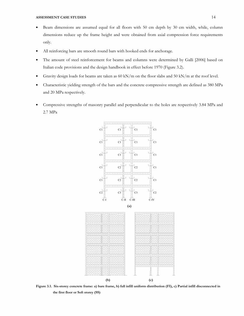
ASSESSMENT CASE STUDIES 14
• Beam dimensions are assumed equal for all floors with 50 cm depth by 30 cm width, while, column
dimensions reduce up the frame height and were obtained from axial compression force requirements
only.
• All reinforcing bars are smooth round bars with hooked ends for anchorage.
• The amount of steel reinforcement for beams and columns were determined by Galli [2006] based on
Italian code provisions and the design handbook in effect before 1970 (Figure 3.2).
• Gravity design loads for beams are taken as 60 kN/m on the floor slabs and 50 kN/m at the roof level.
• Characteristic yielding strength of the bars and the concrete compressive strength are defined as 380 MPa
and 20 MPa respectively.
• Compressive strengths of masonry parallel and perpendicular to the holes are respectively 3.84 MPa and
2.7 MPa
(a)
(b) (c)
Figure 3.1. Six-storey concrete frame: a) bare frame, b) full infill uniform distribution (FI), c) Partial infill disconnected in
the first floor or Soft storey (SS)
C2 C3 C3 C2
C1 C2 C2 C1
C1 C2 C2 C1
C1 C1 C1 C1
C1 C1 C1 C1
C1 C1 C1 C1
C-I C-II C-III C-IV
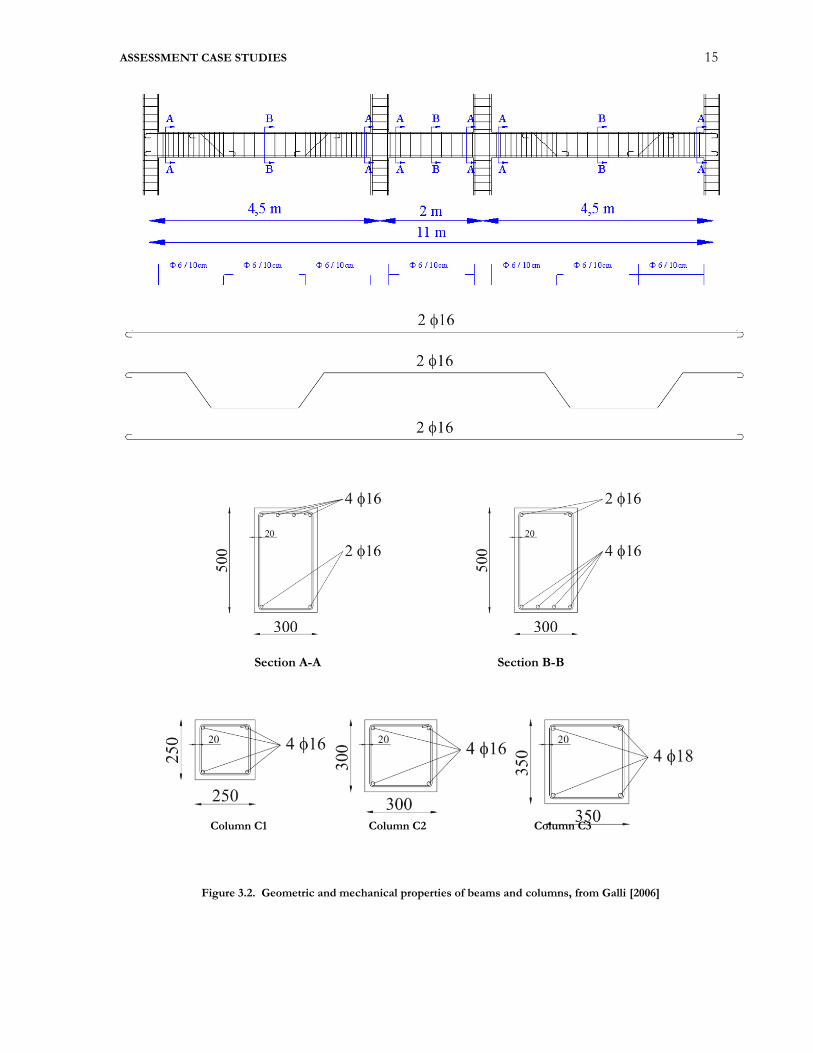
ASSESSMENT CASE STUDIES 15
Figure 3.2. Geometric and mechanical properties of beams and columns, from Galli [2006]
Section A-A Section B-B
Column C1 Column C2 Column C3

ASSESSMENT CASE STUDIES 16
3.3 MODELLING APPROACH
In order to permit the development of the various possible failure mechanisms in the model, care should be
taken in the modelling approach. For the case of RC frames, in addition to allowing beam hinging, it is
important to adequately capture the effects of axial load-moment interaction in columns, masonry infill
failure, and joint failure. The following sections discuss the methodology that is used for the modelling of
components of the case study RC frame.
3.3.1 Modelling of beams and columns
Several approaches are available in the literature to model the nonlinear behaviour of structural elements,
which are differentiated depending on the distribution of the plasticity through the member cross sections
and along its length. For simulating the inelastic response of beam-columns, two general idealized models can
be found in the literature; distributed plasticity and concentrated plasticity. The former approach is
subcategorized to three methodologies as finite length hinge zone, fibre section or finite element, while the
latter could be found in the form of the lumped plastic hinge or the nonlinear spring hinge [Deierlein et al.
2010]. Among them, the fibre element and the lumped plastic hinge are the most common approaches that
are used for modelling of structural elements.
The fibre element model allows representation of details of the geometry and material properties of members
and enables the description of the history of stresses and strains at fibres along the length or across the
section dimensions. The sectional stress-strain is obtained through the integration of the nonlinear uniaxial
material response of the individual fibres, in which the section area of the element is subdivided into finite
regions referred to fibers. The number of fibres depends on the type of the section, the target of the analysis
and the level of accuracy that one wants to achieve. However, to achieve a high level of accuracy, a high
level of knowledge of mechanical and geometrical properties of the structural elements is required. As a
results of high level of uncertainties in a real building, this may lead into a significant error. In addition, it is an
expensive approach due to high computational demands.
The lumped plasticity model concentrates inelastic deformations at the two ends of the member. Beams and
columns are modelled using the Giberson one-component model [Sharpe, 1974]. The stiffness of the hinge is
characterised using the appropriate moment-curvature hysteretic rule over a predefined plastic hinge length.
Such elements have a relatively condensed numerically efficient formulation, and thus, it is the simplest
approach for frame structures. To take into account the effect of axial load variation on the capacity of the
column elements, the M-N interaction diagram is defined. Furthermore, strength degradation curves, which
are a function of the number of cycles or ductility demand, can be associated to the chosen hysteretic rule to
consider the increasing loss of strength in elements that experience in-elastic deformations.
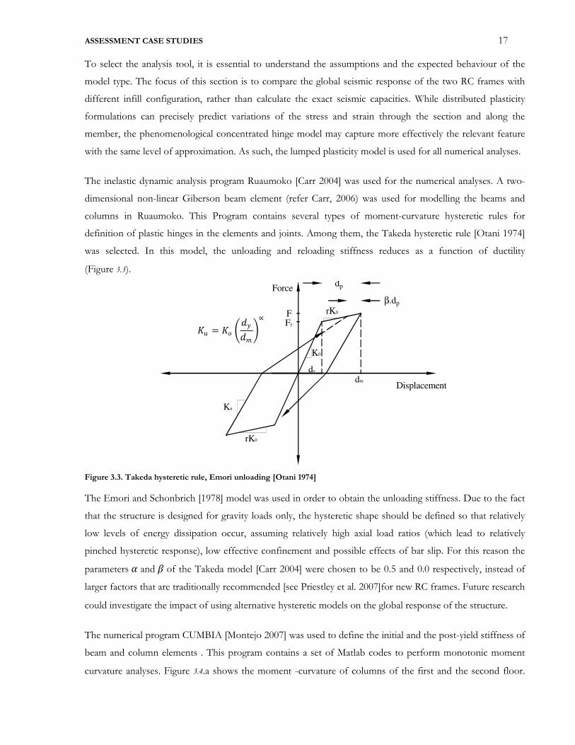
ASSESSMENT CASE STUDIES 17
To select the analysis tool, it is essential to understand the assumptions and the expected behaviour of the
model type. The focus of this section is to compare the global seismic response of the two RC frames with
different infill configuration, rather than calculate the exact seismic capacities. While distributed plasticity
formulations can precisely predict variations of the stress and strain through the section and along the
member, the phenomenological concentrated hinge model may capture more effectively the relevant feature
with the same level of approximation. As such, the lumped plasticity model is used for all numerical analyses.
The inelastic dynamic analysis program Ruaumoko [Carr 2004] was used for the numerical analyses. A two-
dimensional non-linear Giberson beam element (refer Carr, 2006) was used for modelling the beams and
columns in Ruaumoko. This Program contains several types of moment-curvature hysteretic rules for
definition of plastic hinges in the elements and joints. Among them, the Takeda hysteretic rule [Otani 1974]
was selected. In this model, the unloading and reloading stiffness reduces as a function of ductility
(Figure 3.3).
Figure 3.3. Takeda hysteretic rule, Emori unloading [Otani 1974]
The Emori and Schonbrich [1978] model was used in order to obtain the unloading stiffness. Due to the fact
that the structure is designed for gravity loads only, the hysteretic shape should be defined so that relatively
low levels of energy dissipation occur, assuming relatively high axial load ratios (which lead to relatively
pinched hysteretic response), low effective confinement and possible effects of bar slip. For this reason the
parameters � and � of the Takeda model [Carr 2004] were chosen to be 0.5 and 0.0 respectively, instead of
larger factors that are traditionally recommended [see Priestley et al. 2007]for new RC frames. Future research
could investigate the impact of using alternative hysteretic models on the global response of the structure. The numerical program CUMBIA [Montejo 2007] was used to define the initial and the post-yield stiffness of
beam and column elements . This program contains a set of Matlab codes to perform monotonic moment
curvature analyses. Figure 3.4.a shows the moment -curvature of columns of the first and the second floor.
Displacement
FFy
dy
dm
Ku
rK0
rK0
dp
β.dp
K0
Force
� = � ����� �∝
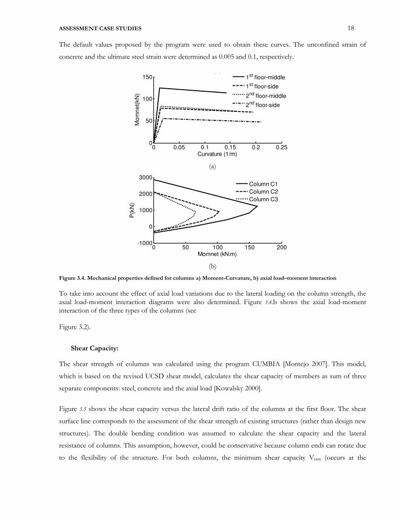
ASSESSMENT CASE STUDIES 18
The default values proposed by the program were used to obtain these curves. The unconfined strain of
concrete and the ultimate steel strain were determined as 0.005 and 0.1, respectively.
(a)
(b)
Figure 3.4. Mechanical properties defined for columns a) Moment-Curvature, b) axial load–moment interaction
To take into account the effect of axial load variations due to the lateral loading on the column strength, the axial load-moment interaction diagrams were also determined. Figure 3.4.b shows the axial load-moment interaction of the three types of the columns (see
Figure 3.2).
Shear Capacity:
The shear strength of columns was calculated using the program CUMBIA [Montejo 2007]. This model,
which is based on the revised UCSD shear model, calculates the shear capacity of members as sum of three
separate components: steel, concrete and the axial load [Kowalsky 2000].
Figure 3.5 shows the shear capacity versus the lateral drift ratio of the columns at the first floor. The shear
surface line corresponds to the assessment of the shear strength of existing structures (rather than design new
structures). The double bending condition was assumed to calculate the shear capacity and the lateral
resistance of columns. This assumption, however, could be conservative because column ends can rotate due
to the flexibility of the structure. For both columns, the minimum shear capacity Vmin (occurs at the
0 0.05 0.1 0.15 0.2 0.250
50
100
150
Curvature (1/m)
Mo
mn
et(
kN
)
(b)
1st floor-middle
1st floor-side
2nd floor-middle
2nd floor-side
0 50 100 150 200-1000
0
1000
2000
3000
Momnet (kN.m)
P(k
N)
Column C1
Column C2
Column C3
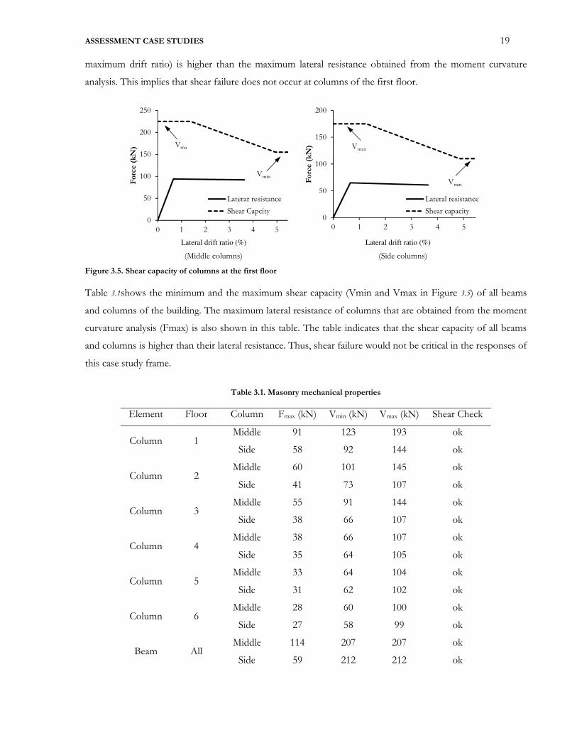
ASSESSMENT CASE STUDIES 19
maximum drift ratio) is higher than the maximum lateral resistance obtained from the moment curvature
analysis. This implies that shear failure does not occur at columns of the first floor.
Lateral drift ratio (%) Lateral drift ratio (%)
(Middle columns) (Side columns)
Figure 3.5. Shear capacity of columns at the first floor
Table 3.1shows the minimum and the maximum shear capacity (Vmin and Vmax in Figure 3.5) of all beams
and columns of the building. The maximum lateral resistance of columns that are obtained from the moment
curvature analysis (Fmax) is also shown in this table. The table indicates that the shear capacity of all beams
and columns is higher than their lateral resistance. Thus, shear failure would not be critical in the responses of
this case study frame.
Table 3.1. Masonry mechanical properties
Element Floor Column Fmax (kN) Vmin (kN) Vmax (kN) Shear Check
Column 1 Middle 91 123 193 ok
Side 58 92 144 ok
Column 2 Middle 60 101 145 ok
Side 41 73 107 ok
Column 3 Middle 55 91 144 ok
Side 38 66 107 ok
Column 4 Middle 38 66 107 ok
Side 35 64 105 ok
Column 5 Middle 33 64 104 ok
Side 31 62 102 ok
Column 6 Middle 28 60 100 ok
Side 27 58 99 ok
Beam All Middle 114 207 207 ok
Side 59 212 212 ok
0
50
100
150
200
250
0 1 2 3 4 5
Force (kN)
Laterar resistance
Shear Capcity
Vma
Vmin
0
50
100
150
200
0 1 2 3 4 5
Force (kN)
x 0.0275
Lateral resistance
Shear capacity
Vmin
Vmax
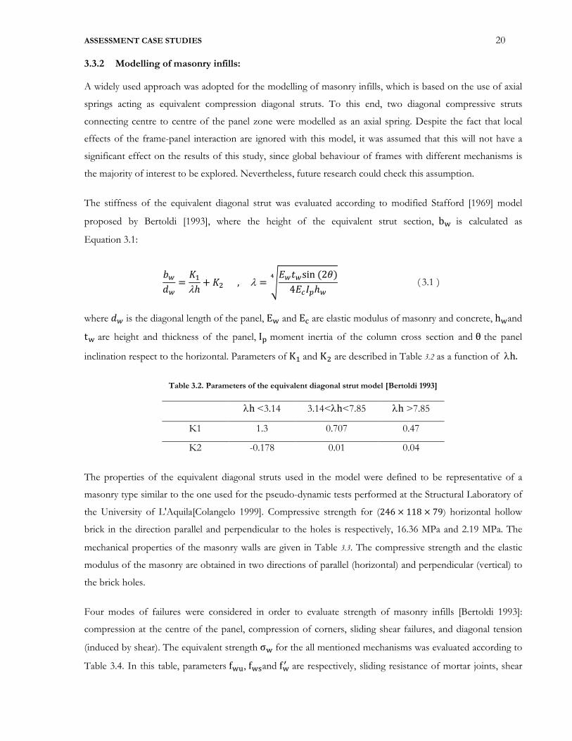
ASSESSMENT CASE STUDIES 20
3.3.2 Modelling of masonry infills:
A widely used approach was adopted for the modelling of masonry infills, which is based on the use of axial
springs acting as equivalent compression diagonal struts. To this end, two diagonal compressive struts
connecting centre to centre of the panel zone were modelled as an axial spring. Despite the fact that local
effects of the frame-panel interaction are ignored with this model, it was assumed that this will not have a
significant effect on the results of this study, since global behaviour of frames with different mechanisms is
the majority of interest to be explored. Nevertheless, future research could check this assumption.
The stiffness of the equivalent diagonal strut was evaluated according to modified Stafford [1969] model
proposed by Bertoldi [1993], where the height of the equivalent strut section, b� is calculated as
Equation 3.1:
���� = �λℎ + � , λ = � �!�sin (2')4 *+,ℎ�
- ( 3.1 )
where �� is the diagonal length of the panel, E� and E/ are elastic modulus of masonry and concrete, h�and
t� are height and thickness of the panel, I3 moment inertia of the column cross section and θ the panel
inclination respect to the horizontal. Parameters of K� and K� are described in Table 3.2 as a function of λh. Table 3.2. Parameters of the equivalent diagonal strut model [Bertoldi 1993]
λh <3.14 3.14<λh<7.85 λh >7.85
K1 1.3 0.707 0.47
K2 -0.178 0.01 0.04
The properties of the equivalent diagonal struts used in the model were defined to be representative of a
masonry type similar to the one used for the pseudo-dynamic tests performed at the Structural Laboratory of
the University of L'Aquila[Colangelo 1999]. Compressive strength for (246 × 118 × 79) horizontal hollow
brick in the direction parallel and perpendicular to the holes is respectively, 16.36 MPa and 2.19 MPa. The
mechanical properties of the masonry walls are given in Table 3.3. The compressive strength and the elastic
modulus of the masonry are obtained in two directions of parallel (horizontal) and perpendicular (vertical) to
the brick holes.
Four modes of failures were considered in order to evaluate strength of masonry infills [Bertoldi 1993]:
compression at the centre of the panel, compression of corners, sliding shear failures, and diagonal tension
(induced by shear). The equivalent strength σ� for the all mentioned mechanisms was evaluated according to
Table 3.4. In this table, parameters f�=, f�>and f�? are respectively, sliding resistance of mortar joints, shear
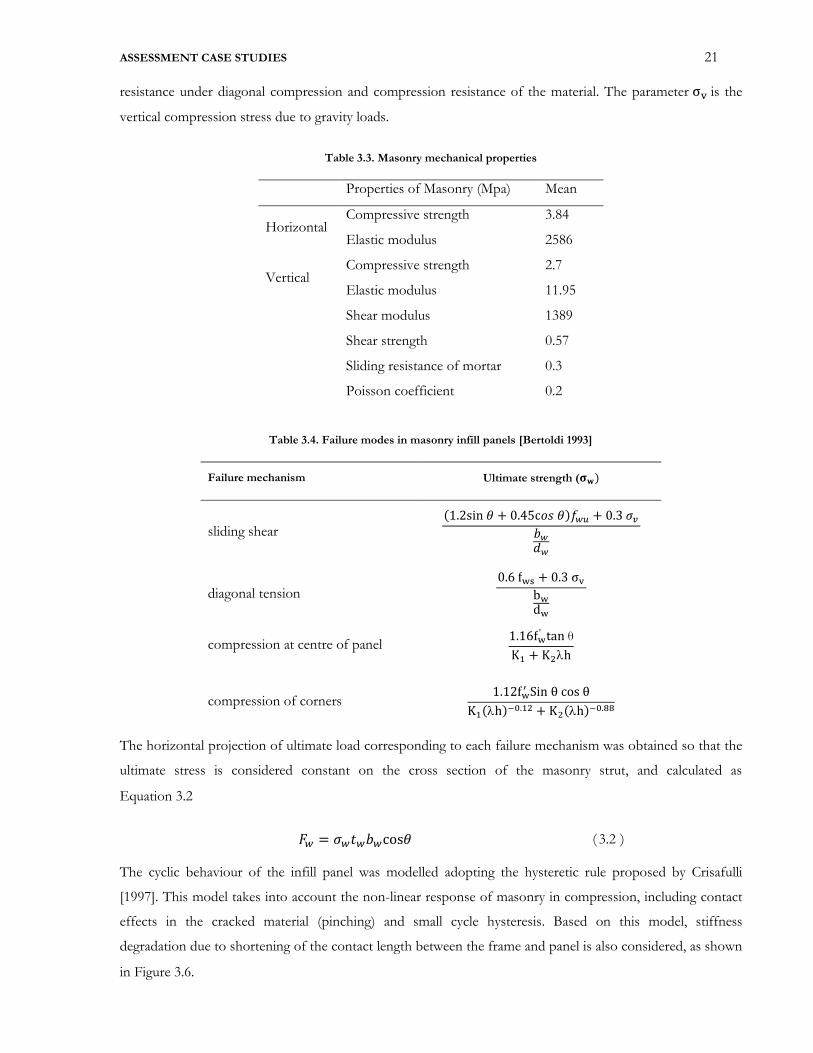
ASSESSMENT CASE STUDIES 21
resistance under diagonal compression and compression resistance of the material. The parameter σ@ is the
vertical compression stress due to gravity loads.
Table 3.3. Masonry mechanical properties
Properties of Masonry (Mpa) Mean
Horizontal Compressive strength 3.84
Elastic modulus 2586
Vertical Compressive strength 2.7
Elastic modulus 11.95
Shear modulus 1389
Shear strength 0.57
Sliding resistance of mortar 0.3
Poisson coefficient 0.2
Table 3.4. Failure modes in masonry infill panels [Bertoldi 1993]
Failure mechanism Ultimate strength (AB)
sliding shear (1.2sin ' + 0.45c�E ')F�G + 0.3 H����
diagonal tension 0.6 f�> + 0.3 σ@b�d�
compression at centre of panel 1.16f�′ tan θK� + K�λh
compression of corners 1.12f�? Sin θ cos θK�(λh)M�.�� + K�(λh)M�.NN
The horizontal projection of ultimate load corresponding to each failure mechanism was obtained so that the
ultimate stress is considered constant on the cross section of the masonry strut, and calculated as
Equation 3.2
O� = �!���cos' ( 3.2 )
The cyclic behaviour of the infill panel was modelled adopting the hysteretic rule proposed by Crisafulli
[1997]. This model takes into account the non-linear response of masonry in compression, including contact
effects in the cracked material (pinching) and small cycle hysteresis. Based on this model, stiffness
degradation due to shortening of the contact length between the frame and panel is also considered, as shown
in Figure 3.6.
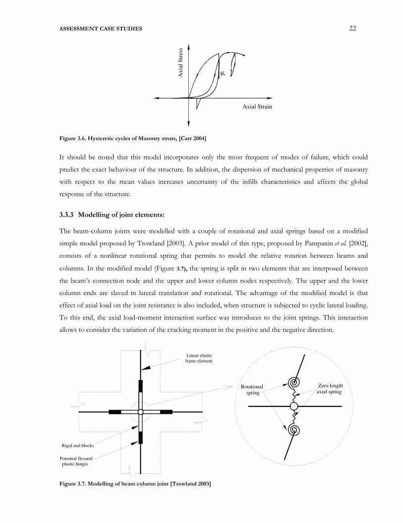
ASSESSMENT CASE STUDIES 22
Figure 3.6. Hysteretic cycles of Masonry struts, [Carr 2004]
It should be noted that this model incorporates only the most frequent of modes of failure, which could
predict the exact behaviour of the structure. In addition, the dispersion of mechanical properties of masonry
with respect to the mean values increases uncertainty of the infills characteristics and affects the global
response of the structure.
3.3.3 Modelling of joint elements:
The beam-column joints were modelled with a couple of rotational and axial springs based on a modified
simple model proposed by Trowland [2003]. A prior model of this type, proposed by Pampanin et al. [2002],
consists of a nonlinear rotational spring that permits to model the relative rotation between beams and
columns. In the modified model (Figure 3.7), the spring is split in two elements that are interposed between
the beam’s connection node and the upper and lower column nodes respectively. The upper and the lower
column ends are slaved in lateral translation and rotational. The advantage of the modified model is that
effect of axial load on the joint resistance is also included, when structure is subjected to cyclic lateral loading.
To this end, the axial load-moment interaction surface was introduces to the joint springs. This interaction
allows to consider the variation of the cracking moment in the positive and the negative direction.
Figure 3.7. Modelling of beam column joint [Trowland 2003]
γE
Axial Strain
Ax
ial
Str
ess
Linear elastic
frame element
Rigid end blocks
Potential flexural
plastic hinges
Zero length
axial spring Rotational
spring

ASSESSMENT CASE STUDIES 23
The moment-rotation relationship of the rotational spring was obtained based on experimental tests
implemented by Pampanin et al. [2002]. A relation between the shear deformation and the principal tensile
stress was found and transformed into the moment-rotation relationship. It was assumed that the shear
deformation of the joint panel is equal to the rotation of the spring. The moment was calculated from the
principal of tensile stress evaluated based on the Mohr theory. According to the test results [Pampanin et al.
2002], the principal tensile stress at first cracking was defined as P. QRST? and P. QURST? for exterior and
interior joints, respectively (Figure 3.8). Hardening behaviour for post-cracked area was assumed for interior
joints up to P. VQRST?, while elasto-plastic behaviour model was adopted for exterior joints.
The spring elements used were identical and they both had half of the joint strength and stiffness. The elastic
axial and rotational stiffness of the joint spring was calculated from:
W = *X*Y , Z = [* \ 0.9�]^^ − 0.9�]` X* ( 3.3 )
where ab and cb are concrete elastic and shear modulus, dT is the column cross section area, e , fg and h
are inter-storey height, beam depth and half of joint panel height, respectively.
Figure 3.8. Monotonic and cyclic behaviour of shear hinge joint model, [Pampanin et al. 2002]

ASSESSMENT CASE STUDIES 24
Figure 3.9. Pampanin Hysteretic rule used in Ruaumoko, [Carr 2004]
The cyclic behaviour of the joint rotational spring was defined using a hysteretic rule available in Ruaumoko
program and specifically proposed to describe the characteristics of the joint response. In particular, the
adopted hysteretic loop is able to describe the typical "pinching" effect due to the slippage of plain round
reinforcing bars through the joint panel zone and to the opening and closing of diagonal shear cracks in the
joint region. As it can be seen in Figure 3.9, the hysteretic rule needs the definition of some parameters
governing the unloading and reloading phases of the cycle.
3.4 GROUND MOTION USED FOR TIME HISTORY ANALYSIS
Time history analyses were carried out using ten recorded horizontal accelerograms selected as part of the
DISTEEL project [Maley et al. 2013]. The record set consisted of 10 records that were scaled to be
compatible with Eurocode 8 spectrum [CEN 2004] for soil type C and a corner period Td = 8s. Figure 3.10
shows the acceleration and displacement response spectra of the selected records. The records show a good
fit with the EC8 design displacement spectrum (shown for a peak ground acceleration (PGA) on rock of
0.4g) but they drop below the design acceleration spectrum in the low period range (T< 1s). This variation is
evident from the COV of 0.553 for the short period range. In comparison, the COV for the medium and
long period ranges are 0.262 and 0.182 respectively. Table 3.5 lists all earthquake records used in the time
rK0
Kα2
Ks2
Kα1
Ks1
Ks1
K0
rKo
Ks2
dpβ.dp
Kα2
Kα1∆F
∆F
F
∆
Parameter T1 T2 L1 C2 �E1 1.2 1.3 1.3 1.2 ij 1.5 1.3 1.4 1.3 ��1 -0.1 -0.1 -0.1 -0.1 ��2 0.9 0.8 0.8 0.95 ∆O 30 30 20 30 � -0.2 -0.3 -0.1 0
l� = m/olG�
l� = m/olG�
p� = m/olp� p� = m/olp�
p� = m/olp�

ASSESSMENT CASE STUDIES 25
history analysis and includes the event magnitude (M), scaling factor and scaled PGA required to obtain
compatibility with the EC8 spectrum constructed at a PGA of 0.4g.
Table 3.5. Record Set used for nonlinear time history analysis
No. Earthquake M Distance
(km)
Scaling
Factor
Scaled
PGA (g)
EQ 01 Chi-Chi, Taiwan 7.62 36 2.1 0.14
EQ 02 Kocaeli 7.51 127 7.9 0.70
EQ 03 Landers 7.28 157 4 0.21
EQ 04 Hector 7.13 92 2.9 0.29
EQ 05 St Elias, Alaska 7.54 80 1.5 0.24
EQ 06 Loma Prieta* 6.93 28 1.8 0.45
EQ 07 Northridge-01 6.69 52 5.8 0.32
EQ 08 Superstition Hills-02 6.54 13 2.3 0.49
EQ 09 Imperial Valley-06 6.53 22 5.1 0.71
EQ 10 Chi-Chi, Taiwan-03 6.2 40 5.6 0.38
In order to run Incremental Dynamic Analyses (IDA) nine different hazard levels are used for the set of
records with the following peak ground accelerations for each intensity level: 0.05g, 0.10g, 0.15g, 0.20g, 0.25g,
0.30g, 0.35g, 0.40g, and 0.60g. As such, 90 non-linear time-history (NLTH) analyses were run for each
building.
3.5 ANALYTICAL RESULTS
Response parameters of interest such as the peak inter storey drift ratio , the peak floor acceleration and the
residual inter storey drift ratio are plotted versus the intensity of the ground motions. In order to estimate the
mean response of all ground motions, the geometric mean value (defined as per [Shome 1999]) using
Equation 3.4 is adopted. The geometric mean is a logical estimation of the median especially if the data are
sampled from lognormal distribution [Benjamin and Cornell 1970].
xr = exp[∑ ln xxyxz�{| ] ( 3.4 )
where x~ geometric means value and n is is the number of observations. The response of each variant is
described in the following sections.

ASSESSMENT CASE STUDIES 26
Figure 3.10. Acceleration and displacement Response Spectra for the selected records sets
3.5.1 Variant 1: Uniform Distribution of Infills (FI)
The natural first period of the full infill case is 0.328 sec, which represents to some extent a stiff structure.
Results of nonlinear time history analysis are presented in the following graphs. Figure 3.11 to Figure 3.14
present response parameters of interest, which include maximum storey drift, residual drift storey, and
maximum floor acceleration at each intensity (hazard) level. The dashed lines represent the responses from
each individual earthquake, while the solid thick line provides the geometric mean values calculated from
Equation 3.4.
The peak floor accelerations over the building height are presented in Figure 3.11. At the range of low
intensity levels (PGA less than 0.2g), the plot indicates a linear distribution of the acceleration over the height.
However, when the intensity increases, the distribution is changed. For the range of high intensity levels,
more than 0.35g, the acceleration is almost uniform through the building height. This is likely because the soft
storey mechanism is formed, as explained in the next paragraph.
0
0.5
1
1.5
2
2.5
3
0 2 4 6 8A
cce
lera
tio
n (
g)
Period (s)
Earthquakes
Design
Mean
0
50
100
150
200
0 2 4 6 8
Dis
pla
cem
en
t (c
m)
Period (s)
Earthquakes
Design
Mean
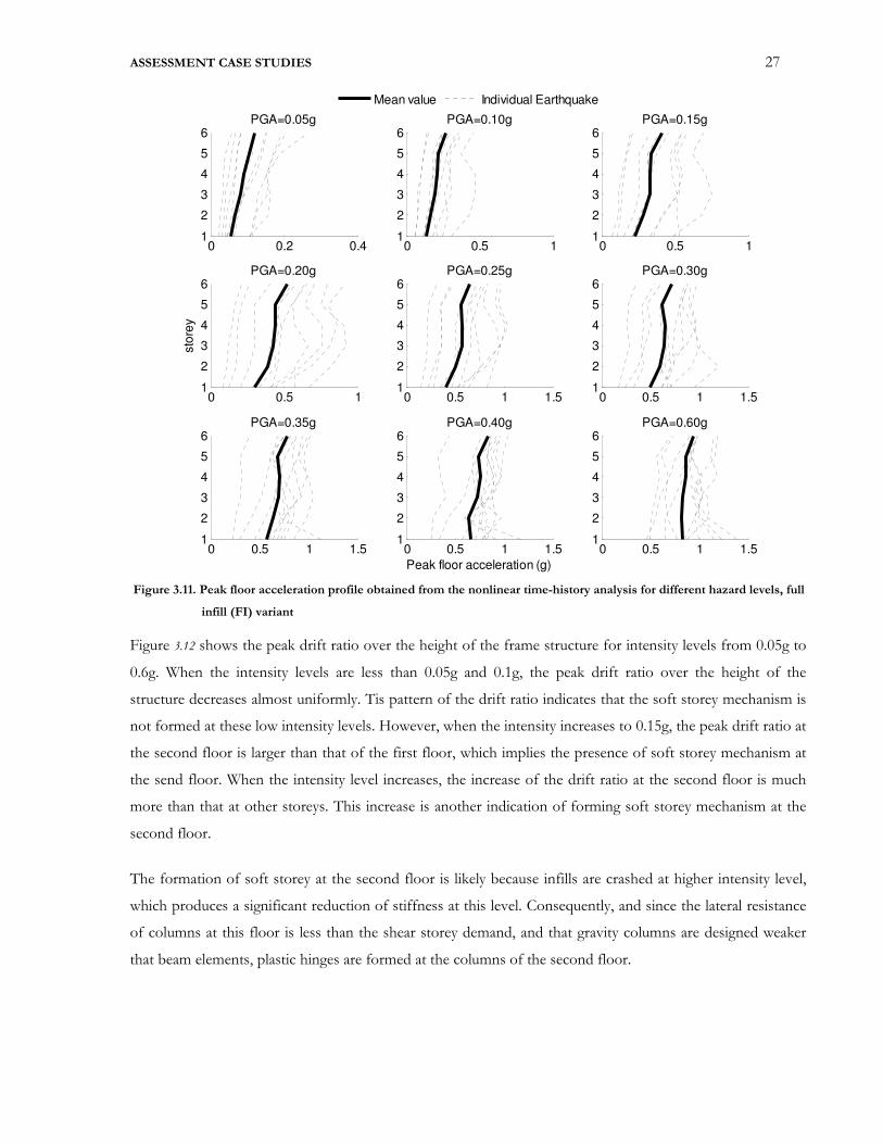
ASSESSMENT CASE STUDIES 27
Figure 3.11. Peak floor acceleration profile obtained from the nonlinear time-history analysis for different hazard levels, full
infill (FI) variant
Figure 3.12 shows the peak drift ratio over the height of the frame structure for intensity levels from 0.05g to
0.6g. When the intensity levels are less than 0.05g and 0.1g, the peak drift ratio over the height of the
structure decreases almost uniformly. Tis pattern of the drift ratio indicates that the soft storey mechanism is
not formed at these low intensity levels. However, when the intensity increases to 0.15g, the peak drift ratio at
the second floor is larger than that of the first floor, which implies the presence of soft storey mechanism at
the send floor. When the intensity level increases, the increase of the drift ratio at the second floor is much
more than that at other storeys. This increase is another indication of forming soft storey mechanism at the
second floor.
The formation of soft storey at the second floor is likely because infills are crashed at higher intensity level,
which produces a significant reduction of stiffness at this level. Consequently, and since the lateral resistance
of columns at this floor is less than the shear storey demand, and that gravity columns are designed weaker
that beam elements, plastic hinges are formed at the columns of the second floor.
0 0.2 0.41
2
3
4
5
6PGA=0.05g
0 0.5 11
2
3
4
5
6PGA=0.10g
0 0.5 11
2
3
4
5
6PGA=0.15g
0 0.5 11
2
3
4
5
6PGA=0.20g
sto
rey
0 0.5 1 1.51
2
3
4
5
6PGA=0.25g
0 0.5 1 1.51
2
3
4
5
6PGA=0.30g
0 0.5 1 1.51
2
3
4
5
6PGA=0.35g
0 0.5 1 1.51
2
3
4
5
6PGA=0.40g
Peak floor acceleration (g)
0 0.5 1 1.51
2
3
4
5
6PGA=0.60g
Mean value Individual Earthquake
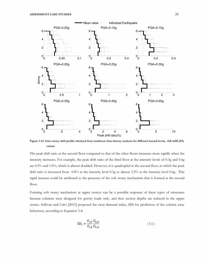
ASSESSMENT CASE STUDIES 28
Figure 3.12. Inter storey drift profile obtained from nonlinear time-history analysis for different hazard levels, full infill (FI)
variant
The peak drift ratio at the second floor compared to that of the other floors increases more rapidly when the
intensity increases. For example, the peak drift ratio of the third floor at the intensity levels of 0.3g and 0.6g
are 0.5% and 1.0%, which is almost doubled. However, it is quadrupled at the second floor, in which the peak
drift ratio is increased from 0.8% at the intensity level 0.3g to almost 3.2% at the intensity level 0.6g. This
rapid increase could be attributed to the presence of the soft storey mechanism that is formed at the second
floor.
Forming soft storey mechanism at upper storeys can be a possible response of these types of structures
because columns were designed for gravity loads only, and thus section depths are reduced in the upper
stories. Sullivan and Calvi [2011] proposed the sway-demand index, SDi for prediction of the column sway
behaviour, according to Equation 3.4:
SDx = ��,���,��],��],� ( 3.5 )
0 0.05 0.10
2
4
6PGA=0.05g
0 0.2 0.40
2
4
6PGA=0.10g
0 0.2 0.40
2
4
6PGA=0.15g
0 0.5 10
2
4
6PGA=0.20g
sto
rey
0 1 20
2
4
6PGA=0.25g
0 1 2 30
2
4
6PGA=0.30g
0 2 40
2
4
6PGA=0.35g
0 2 4 60
2
4
6PGA=0.40g
Peak drift ratio(%)
0 5 100
2
4
6PGA=0.60g
Mean value Individual Earthquake
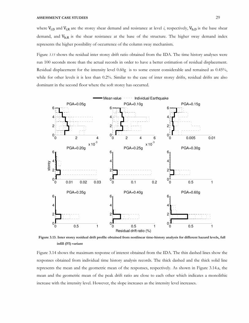
ASSESSMENT CASE STUDIES 29
where Vx.� and Vx,� are the storey shear demand and resistance at level i, respectively, V�,� is the base shear
demand, and V�,� is the shear resistance at the base of the structure. The higher sway demand index
represents the higher possibility of occurrence of the column sway mechanism.
Figure 3.13 shows the residual inter storey drift ratio obtained from the IDA. The time history analyses were
run 100 seconds more than the actual records in order to have a better estimation of residual displacement.
Residual displacement for the intensity level 0.60g is to some extent considerable and remained as 0.45%,
while for other levels it is less than 0.2%. Similar to the case of inter storey drifts, residual drifts are also
dominant in the second floor where the soft storey has occurred.
Figure 3.13. Inter storey residual drift profile obtained from nonlinear time-history analysis for different hazard levels, full
infill (FI) variant
Figure 3.14 shows the maximum response of interest obtained from the IDA. The thin dashed lines show the
responses obtained from individual time history analysis records. The thick dashed and the thick solid line
represents the mean and the geometric mean of the responses, respectively. As shown in Figure 3.14.a, the
mean and the geometric mean of the peak drift ratio are close to each other which indicates a monolithic
increase with the intensity level. However, the slope increases as the intensity level increases.
0 2 4
x 10-3
0
2
4
6PGA=0.05g
0 2 4 6
x 10-3
0
2
4
6PGA=0.10g
0 0.005 0.010
2
4
6PGA=0.15g
0 0.01 0.02 0.030
2
4
6PGA=0.20g
sto
rey
0 0.1 0.20
2
4
6PGA=0.25g
0 0.5 10
2
4
6PGA=0.30g
0 0.5 10
2
4
6PGA=0.35g
0 0.5 10
2
4
6PGA=0.40g
Residual drift ratio (%)
0 0.5 10
2
4
6PGA=0.60g
Mean value Individual Earthquake

ASSESSMENT CASE STUDIES 30
This trend is to somehow different for residual drift ratio (Figure 3.14.b), which is almost zero for the
intensity levels below 0.2g, and then, it increases rapidly. The classic mean value calculates the average of all
individual responses better than the geometric mean value. That is likely due to the presence of zero residual
drift ratio (or very low values) that are obtained from some ground motions. That could create misleading
values in the logarithmic calculations. Thus, the geometric mean value could not be an appropriate tool to
represent the residual drift ratio, if values are very low.
Figure 3.14. Peak response of interests obtained from incremental dynamic analysis, full infill (FI) variant
Figure 3.14.c presents the IDA curve for the peak floor acceleration, which is increased almost linearly up to
the intensity level of 0.35g. After this level, the slope is decreased as the intensity increases, which could be
due to forming plastic hinges at the second floor. Figure 3.14.d shows the comparison of the peak drift ratio
and the residual drift ratio. Despite the fact that the peak drift ratio at the highest intensity level reaches
almost 3.5%, the peak residual displacement are very low (0.5%). The presence of infills at all floors could be
the reason that the residual displacements are not significant.
3.5.2 Variant 2: Partial Distribution of Infills- Soft First Storey (SS)
In the second case study, the aforementioned frame analysed for a condition that the masonry infills on all
floors are removed at the first floor. Figure 3.15 presents the peak floor acceleration obtained from individual
ground motions as well as the mean values.
0.050.10.150.20.250.30.350.4 0.60
2
4
6
8
Pea
k d
rift r
atio %
PGA(g)
(a)
0.050.10.150.20.250.30.350.4 0.60
0.2
0.4
0.6
0.8
1
Resid
ua
l dri
ft r
atio
%
PGA(g)
(b)
0.050.10.150.20.250.30.350.4 0.60
0.5
1
1.5
Pe
ak flo
or a
cce
lera
tio
n(g
)
PGA(g)
(c)
Mean Geomteric Mean Individual Earthquake
0.050.10.150.20.250.30.350.4 0.60
1
2
3
4
PGA(g)
Pea
k a
nd r
esid
ual d
rift
(d)
Mean Interstory Drift
Mean Interstory Residual Drift
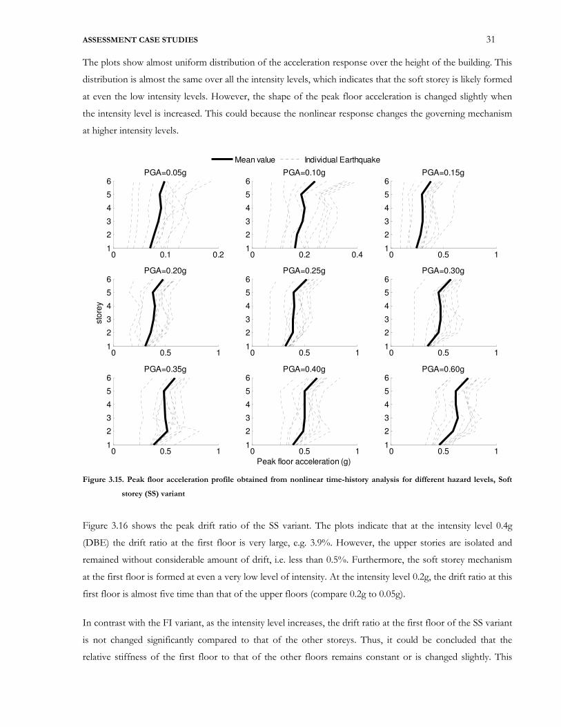
ASSESSMENT CASE STUDIES 31
The plots show almost uniform distribution of the acceleration response over the height of the building. This
distribution is almost the same over all the intensity levels, which indicates that the soft storey is likely formed
at even the low intensity levels. However, the shape of the peak floor acceleration is changed slightly when
the intensity level is increased. This could because the nonlinear response changes the governing mechanism
at higher intensity levels.
Figure 3.15. Peak floor acceleration profile obtained from nonlinear time-history analysis for different hazard levels, Soft
storey (SS) variant
Figure 3.16 shows the peak drift ratio of the SS variant. The plots indicate that at the intensity level 0.4g
(DBE) the drift ratio at the first floor is very large, e.g. 3.9%. However, the upper stories are isolated and
remained without considerable amount of drift, i.e. less than 0.5%. Furthermore, the soft storey mechanism
at the first floor is formed at even a very low level of intensity. At the intensity level 0.2g, the drift ratio at this
first floor is almost five time than that of the upper floors (compare 0.2g to 0.05g).
In contrast with the FI variant, as the intensity level increases, the drift ratio at the first floor of the SS variant
is not changed significantly compared to that of the other storeys. Thus, it could be concluded that the
relative stiffness of the first floor to that of the other floors remains constant or is changed slightly. This
0 0.1 0.21
2
3
4
5
6PGA=0.05g
0 0.2 0.41
2
3
4
5
6PGA=0.10g
0 0.5 11
2
3
4
5
6PGA=0.15g
0 0.5 11
2
3
4
5
6PGA=0.20g
sto
rey
0 0.5 11
2
3
4
5
6PGA=0.25g
0 0.5 11
2
3
4
5
6PGA=0.30g
0 0.5 11
2
3
4
5
6PGA=0.35g
0 0.5 11
2
3
4
5
6PGA=0.40g
Peak floor acceleration (g)
0 0.5 11
2
3
4
5
6PGA=0.60g
Mean value Individual Earthquake
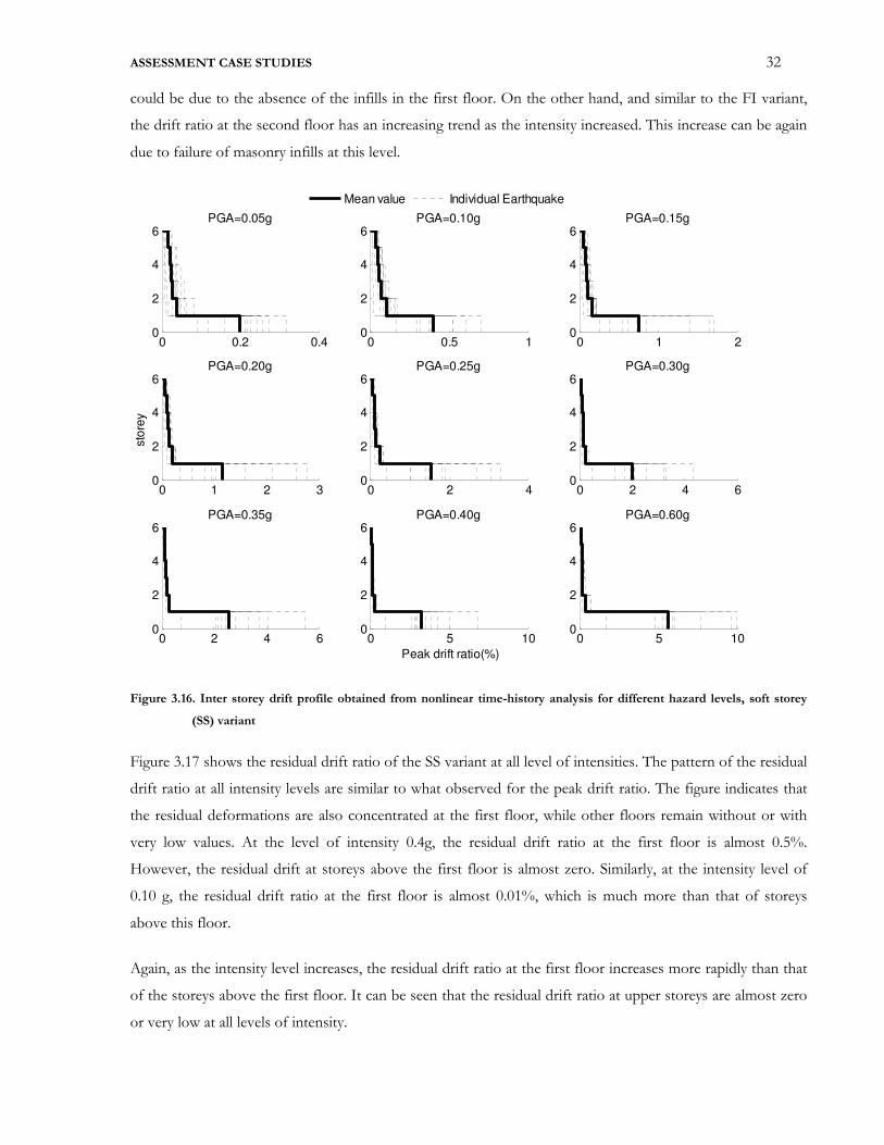
ASSESSMENT CASE STUDIES 32
could be due to the absence of the infills in the first floor. On the other hand, and similar to the FI variant,
the drift ratio at the second floor has an increasing trend as the intensity increased. This increase can be again
due to failure of masonry infills at this level.
Figure 3.16. Inter storey drift profile obtained from nonlinear time-history analysis for different hazard levels, soft storey
(SS) variant
Figure 3.17 shows the residual drift ratio of the SS variant at all level of intensities. The pattern of the residual
drift ratio at all intensity levels are similar to what observed for the peak drift ratio. The figure indicates that
the residual deformations are also concentrated at the first floor, while other floors remain without or with
very low values. At the level of intensity 0.4g, the residual drift ratio at the first floor is almost 0.5%.
However, the residual drift at storeys above the first floor is almost zero. Similarly, at the intensity level of
0.10 g, the residual drift ratio at the first floor is almost 0.01%, which is much more than that of storeys
above this floor.
Again, as the intensity level increases, the residual drift ratio at the first floor increases more rapidly than that
of the storeys above the first floor. It can be seen that the residual drift ratio at upper storeys are almost zero
or very low at all levels of intensity.
0 0.2 0.40
2
4
6PGA=0.05g
0 0.5 10
2
4
6PGA=0.10g
0 1 20
2
4
6PGA=0.15g
0 1 2 30
2
4
6PGA=0.20g
sto
rey
0 2 40
2
4
6PGA=0.25g
0 2 4 60
2
4
6PGA=0.30g
0 2 4 60
2
4
6PGA=0.35g
0 5 100
2
4
6PGA=0.40g
Peak drift ratio(%)
0 5 100
2
4
6PGA=0.60g
Mean value Individual Earthquake

ASSESSMENT CASE STUDIES 33
As a result, the reduction of the residual deformations at storeys above the first floor is another advantage of
forming soft storey at the first floor. However, one should note that the residual drift at the first floor must
be controlled and remain in an acceptable range. Otherwise, the building could not be in a suitable
performance after the earthquake.
Figure 3.17. Residual storey drift profile obtained from nonlinear time-history analysis for different hazard levels, soft storey
(SS) variant
Similar to the FI variant, peak responses from different hazard levels are plotted for the SS variant.
Figure 3.18 shows the IDA curves corresponding to the peak drift ratio, the residual drift ratio and the peak
floor acceleration. In contrast to the FI variant, the mean and the geometric mean values shown in this figure
are closer to each other. As the intensity level increases, the peak floor acceleration increases almost
constantly, whereas the residual displacement has some fluctuations.
In order to find the pattern of the damage and to compare the seismic demand to the capacity of structural
elements, a displacement damage index DDI defined as the following equation is calculated for structural
elements.
��+ = ���� ( 3.6)
0 2 4
x 10-3
0
2
4
6PGA=0.05g
0 0.02 0.040
2
4
6PGA=0.10g
0 0.2 0.40
2
4
6PGA=0.15g
0 0.2 0.40
2
4
6PGA=0.20g
sto
rey
0 0.2 0.40
2
4
6PGA=0.25g
0 0.5 10
2
4
6PGA=0.30g
0 0.5 10
2
4
6PGA=0.35g
0 0.5 1 1.50
2
4
6PGA=0.40g
Residual drift ratio (%)
0 0.5 1 1.50
2
4
6PGA=0.60g
Figure A.4.2. Residual drift ratio, Variant: SS-NPD
Mean value Individual Earthquake
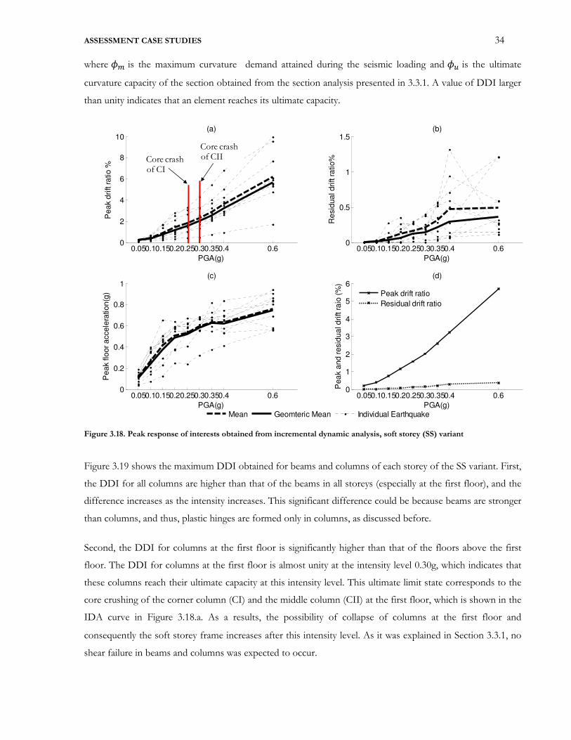
ASSESSMENT CASE STUDIES 34
where �� is the maximum curvature demand attained during the seismic loading and �G is the ultimate
curvature capacity of the section obtained from the section analysis presented in 3.3.1. A value of DDI larger
than unity indicates that an element reaches its ultimate capacity.
Figure 3.18. Peak response of interests obtained from incremental dynamic analysis, soft storey (SS) variant
Figure 3.19 shows the maximum DDI obtained for beams and columns of each storey of the SS variant. First,
the DDI for all columns are higher than that of the beams in all storeys (especially at the first floor), and the
difference increases as the intensity increases. This significant difference could be because beams are stronger
than columns, and thus, plastic hinges are formed only in columns, as discussed before.
Second, the DDI for columns at the first floor is significantly higher than that of the floors above the first
floor. The DDI for columns at the first floor is almost unity at the intensity level 0.30g, which indicates that
these columns reach their ultimate capacity at this intensity level. This ultimate limit state corresponds to the
core crushing of the corner column (CI) and the middle column (CII) at the first floor, which is shown in the
IDA curve in Figure 3.18.a. As a results, the possibility of collapse of columns at the first floor and
consequently the soft storey frame increases after this intensity level. As it was explained in Section 3.3.1, no
shear failure in beams and columns was expected to occur.
0.050.10.150.20.250.30.350.4 0.60
2
4
6
8
10
Pe
ak d
rift r
atio
%
PGA(g)
(a)
0.050.10.150.20.250.30.350.4 0.60
0.5
1
1.5
Re
sid
ua
l dri
ft ra
tio%
PGA(g)
(b)
0.050.10.150.20.250.30.350.4 0.60
0.2
0.4
0.6
0.8
1
Pe
ak flo
or
acce
lera
tion
(g)
PGA(g)
(c)
Mean Geomteric Mean Individual Earthquake
0.050.10.150.20.250.30.350.4 0.60
1
2
3
4
5
6
PGA(g)
Pea
k a
nd
re
sid
ua
l d
rift r
aio
(%
)
(d)
Peak drift ratio
Residual drift ratio
Core crashof CI
Core crashof CII
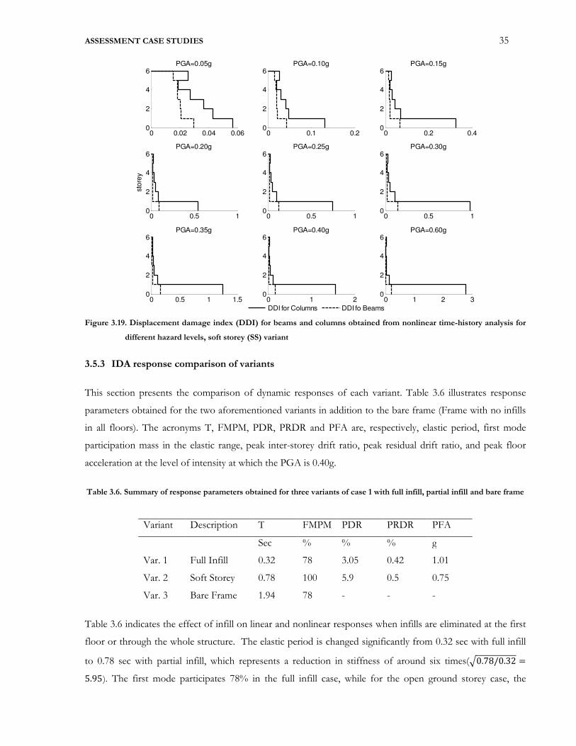
ASSESSMENT CASE STUDIES 35
Figure 3.19. Displacement damage index (DDI) for beams and columns obtained from nonlinear time-history analysis for
different hazard levels, soft storey (SS) variant
3.5.3 IDA response comparison of variants
This section presents the comparison of dynamic responses of each variant. Table 3.6 illustrates response
parameters obtained for the two aforementioned variants in addition to the bare frame (Frame with no infills
in all floors). The acronyms T, FMPM, PDR, PRDR and PFA are, respectively, elastic period, first mode
participation mass in the elastic range, peak inter-storey drift ratio, peak residual drift ratio, and peak floor
acceleration at the level of intensity at which the PGA is 0.40g.
Table 3.6. Summary of response parameters obtained for three variants of case 1 with full infill, partial infill and bare frame
Variant Description T FMPM PDR PRDR PFA
Sec % % % g
Var. 1 Full Infill 0.32 78 3.05 0.42 1.01
Var. 2 Soft Storey 0.78 100 5.9 0.5 0.75
Var. 3 Bare Frame 1.94 78 - - -
Table 3.6 indicates the effect of infill on linear and nonlinear responses when infills are eliminated at the first
floor or through the whole structure. The elastic period is changed significantly from 0.32 sec with full infill
to 0.78 sec with partial infill, which represents a reduction in stiffness of around six times(R0.78/0.32 =5.95). The first mode participates 78% in the full infill case, while for the open ground storey case, the
0 0.02 0.04 0.060
2
4
6PGA=0.05g
0 0.1 0.20
2
4
6PGA=0.10g
0 0.2 0.40
2
4
6PGA=0.15g
0 0.5 10
2
4
6PGA=0.20g
sto
rey
0 0.5 10
2
4
6PGA=0.25g
0 0.5 10
2
4
6PGA=0.30g
0 0.5 1 1.50
2
4
6PGA=0.35g
0 1 20
2
4
6PGA=0.40g
DDI for Columns DDI fo Beams
0 1 2 30
2
4
6PGA=0.60g
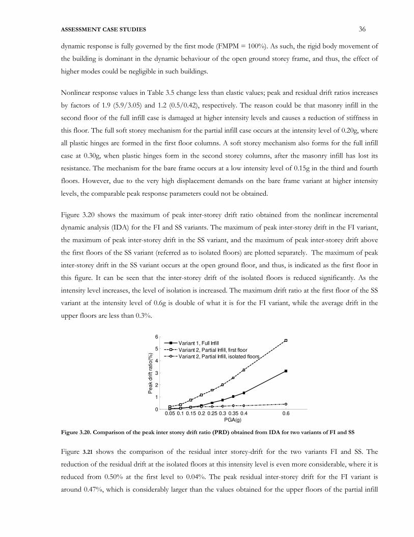
ASSESSMENT CASE STUDIES 36
dynamic response is fully governed by the first mode (FMPM = 100%). As such, the rigid body movement of
the building is dominant in the dynamic behaviour of the open ground storey frame, and thus, the effect of
higher modes could be negligible in such buildings.
Nonlinear response values in Table 3.5 change less than elastic values; peak and residual drift ratios increases
by factors of 1.9 (5.9/3.05) and 1.2 (0.5/0.42), respectively. The reason could be that masonry infill in the
second floor of the full infill case is damaged at higher intensity levels and causes a reduction of stiffness in
this floor. The full soft storey mechanism for the partial infill case occurs at the intensity level of 0.20g, where
all plastic hinges are formed in the first floor columns. A soft storey mechanism also forms for the full infill
case at 0.30g, when plastic hinges form in the second storey columns, after the masonry infill has lost its
resistance. The mechanism for the bare frame occurs at a low intensity level of 0.15g in the third and fourth
floors. However, due to the very high displacement demands on the bare frame variant at higher intensity
levels, the comparable peak response parameters could not be obtained.
Figure 3.20 shows the maximum of peak inter-storey drift ratio obtained from the nonlinear incremental
dynamic analysis (IDA) for the FI and SS variants. The maximum of peak inter-storey drift in the FI variant,
the maximum of peak inter-storey drift in the SS variant, and the maximum of peak inter-storey drift above
the first floors of the SS variant (referred as to isolated floors) are plotted separately. The maximum of peak
inter-storey drift in the SS variant occurs at the open ground floor, and thus, is indicated as the first floor in
this figure. It can be seen that the inter-storey drift of the isolated floors is reduced significantly. As the
intensity level increases, the level of isolation is increased. The maximum drift ratio at the first floor of the SS
variant at the intensity level of 0.6g is double of what it is for the FI variant, while the average drift in the
upper floors are less than 0.3%.
Figure 3.20. Comparison of the peak inter storey drift ratio (PRD) obtained from IDA for two variants of FI and SS
Figure 3.21 shows the comparison of the residual inter storey-drift for the two variants FI and SS. The
reduction of the residual drift at the isolated floors at this intensity level is even more considerable, where it is
reduced from 0.50% at the first level to 0.04%. The peak residual inter-storey drift for the FI variant is
around 0.47%, which is considerably larger than the values obtained for the upper floors of the partial infill
0.05 0.1 0.15 0.2 0.25 0.3 0.35 0.4 0.60
1
2
3
4
5
6
Pe
ak d
rift r
atio
(%)
PGA(g)
Variant 1, Full Infill
Variant 2, Partial Infill, first floor
Variant 2, Partial Infill, isolated floors
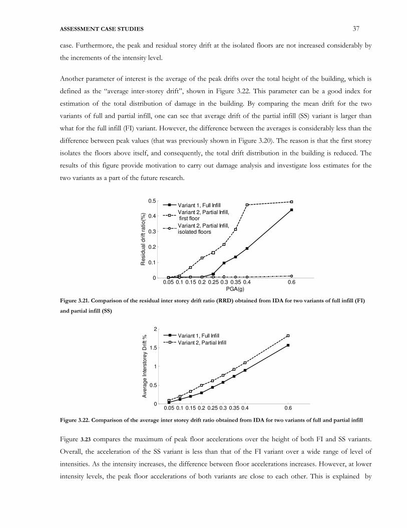
ASSESSMENT CASE STUDIES 37
case. Furthermore, the peak and residual storey drift at the isolated floors are not increased considerably by
the increments of the intensity level.
Another parameter of interest is the average of the peak drifts over the total height of the building, which is
defined as the “average inter-storey drift”, shown in Figure 3.22. This parameter can be a good index for
estimation of the total distribution of damage in the building. By comparing the mean drift for the two
variants of full and partial infill, one can see that average drift of the partial infill (SS) variant is larger than
what for the full infill (FI) variant. However, the difference between the averages is considerably less than the
difference between peak values (that was previously shown in Figure 3.20). The reason is that the first storey
isolates the floors above itself, and consequently, the total drift distribution in the building is reduced. The
results of this figure provide motivation to carry out damage analysis and investigate loss estimates for the
two variants as a part of the future research.
Figure 3.21. Comparison of the residual inter storey drift ratio (RRD) obtained from IDA for two variants of full infill (FI)
and partial infill (SS)
Figure 3.22. Comparison of the average inter storey drift ratio obtained from IDA for two variants of full and partial infill
Figure 3.23 compares the maximum of peak floor accelerations over the height of both FI and SS variants.
Overall, the acceleration of the SS variant is less than that of the FI variant over a wide range of level of
intensities. As the intensity increases, the difference between floor accelerations increases. However, at lower
intensity levels, the peak floor accelerations of both variants are close to each other. This is explained by
0.05 0.1 0.15 0.2 0.25 0.3 0.35 0.4 0.60
0.1
0.2
0.3
0.4
0.5
Resid
ua
l d
rift r
atio
(%)
PGA(g)
Variant 1, Full Infill
Variant 2, Partial Infill, first floor
Variant 2, Partial Infill,isolated floors
0.05 0.1 0.15 0.2 0.25 0.3 0.35 0.4 0.60
0.5
1
1.5
2
Ave
rag
e In
ters
tore
y D
rift %
PGA(g)
Variant 1, Full Infill
Variant 2, Partial Infill
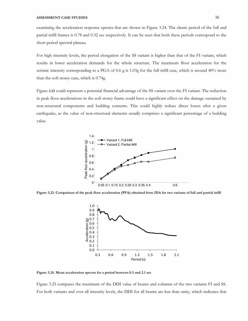
ASSESSMENT CASE STUDIES 38
examining the acceleration response spectra that are shown in Figure 3.24. The elastic period of the full and
partial infill frames is 0.78 and 0.32 sec respectively. It can be seen that both these periods correspond to the
short period spectral plateau.
For high intensity levels, the period elongation of the SS variant is higher than that of the FI variant, which
results in lower acceleration demands for the whole structure. The maximum floor acceleration for the
seismic intensity corresponding to a PGA of 0.6 g is 1.03g for the full infill case, which is around 40% more
than the soft storey case, which is 0.74g.
Figure 3.23 could represent a potential financial advantage of the SS variant over the FI variant. The reduction
in peak floor accelerations in the soft storey frame could have a significant effect on the damage sustained by
non-structural components and building contents. This could highly reduce direct losses after a given
earthquake, as the value of non-structural elements usually comprises a significant percentage of a building
value.
Figure 3.23. Comparison of the peak floor acceleration (PFA) obtained from IDA for two variants of full and partial infill
Figure 3.24. Mean acceleration spectra for a period between 0.3 and 2.1 sec
Figure 3.25 compares the maximum of the DDI value of beams and columns of the two variants FI and SS.
For both variants and over all intensity levels, the DDI for all beams are less than unity, which indicates that
0.05 0.1 0.15 0.2 0.25 0.3 0.35 0.4 0.60
0.2
0.4
0.6
0.8
1
1.2
1.4
Pe
ak flo
or
acce
lera
tio
n (
g)
PGA(g)
Variant 1, Full Infill
Variant 2, Partial Infill
0.0
0.1
0.2
0.3
0.4
0.5
0.6
0.7
0.8
0.9
1.0
0.3 0.6 0.9 1.2 1.5 1.8 2.1
Acc
ele
rati
on
(g
)
Period (s)
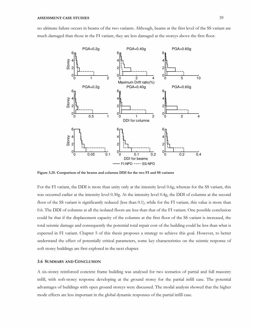
ASSESSMENT CASE STUDIES 39
no ultimate failure occurs in beams of the two variants. Although, beams at the first level of the SS variant are
much damaged than those in the FI variant, they are less damaged at the storeys above the first floor.
Figure 3.25. Comparison of the beams and columns DDI for the two FI and SS variants
For the FI variant, the DDI is more than unity only at the intensity level 0.6g, whereas for the SS variant, this
was occurred earlier at the intensity level 0.30g. At the intensity level 0.4g, the DDI of columns at the second
floor of the SS variant is significantly reduced (less than 0.1), while for the FI variant, this value is more than
0.6. The DDI of columns at all the isolated floors are less than that of the FI variant. One possible conclusion
could be that if the displacement capacity of the columns at the first floor of the SS variant is increased, the
total seismic damage and consequently the potential total repair cost of the building could be less than what is
expected in FI variant. Chapter 5 of this thesis proposes a strategy to achieve this goal. However, to better
understand the effect of potentially critical parameters, some key characteristics on the seismic response of
soft storey buildings are first explored in the next chapter.
3.6 SUMMARY AND CONCLUSION
A six-storey reinforced concrete frame building was analysed for two scenarios of partial and full masonry
infill, with soft-storey response developing at the ground storey for the partial infill case. The potential
advantages of buildings with open ground storeys were discussed. The modal analysis showed that the higher
mode effects are less important in the global dynamic responses of the partial infill case.
0 1 20
2
4
6PGA=0.2g
Sto
rey
0 0.5 10
2
4
6PGA=0.2g
Sto
rey
0 0.05 0.10
2
4
6
Sto
rey
0 2 40
2
4
6PGA=0.40g
Maximum Drift ratio(%)
0 1 20
2
4
6PGA=0.40g
DDI for columns
0 0.1 0.20
2
4
6
DDI for beams
0 5 100
2
4
6PGA=0.60g
0 2 40
2
4
6PGA=0.60g
0 0.2 0.40
2
4
6
FI-NPD SS-NPD
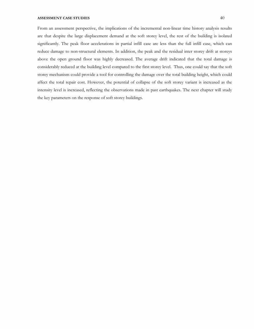
ASSESSMENT CASE STUDIES 40
From an assessment perspective, the implications of the incremental non-linear time history analysis results
are that despite the large displacement demand at the soft storey level, the rest of the building is isolated
significantly. The peak floor accelerations in partial infill case are less than the full infill case, which can
reduce damage to non-structural elements. In addition, the peak and the residual inter storey drift at storeys
above the open ground floor was highly decreased. The average drift indicated that the total damage is
considerably reduced at the building level compared to the first storey level. Thus, one could say that the soft
storey mechanism could provide a tool for controlling the damage over the total building height, which could
affect the total repair cost. However, the potential of collapse of the soft storey variant is increased as the
intensity level is increased, reflecting the observations made in past earthquakes. The next chapter will study
the key parameters on the response of soft storey buildings.
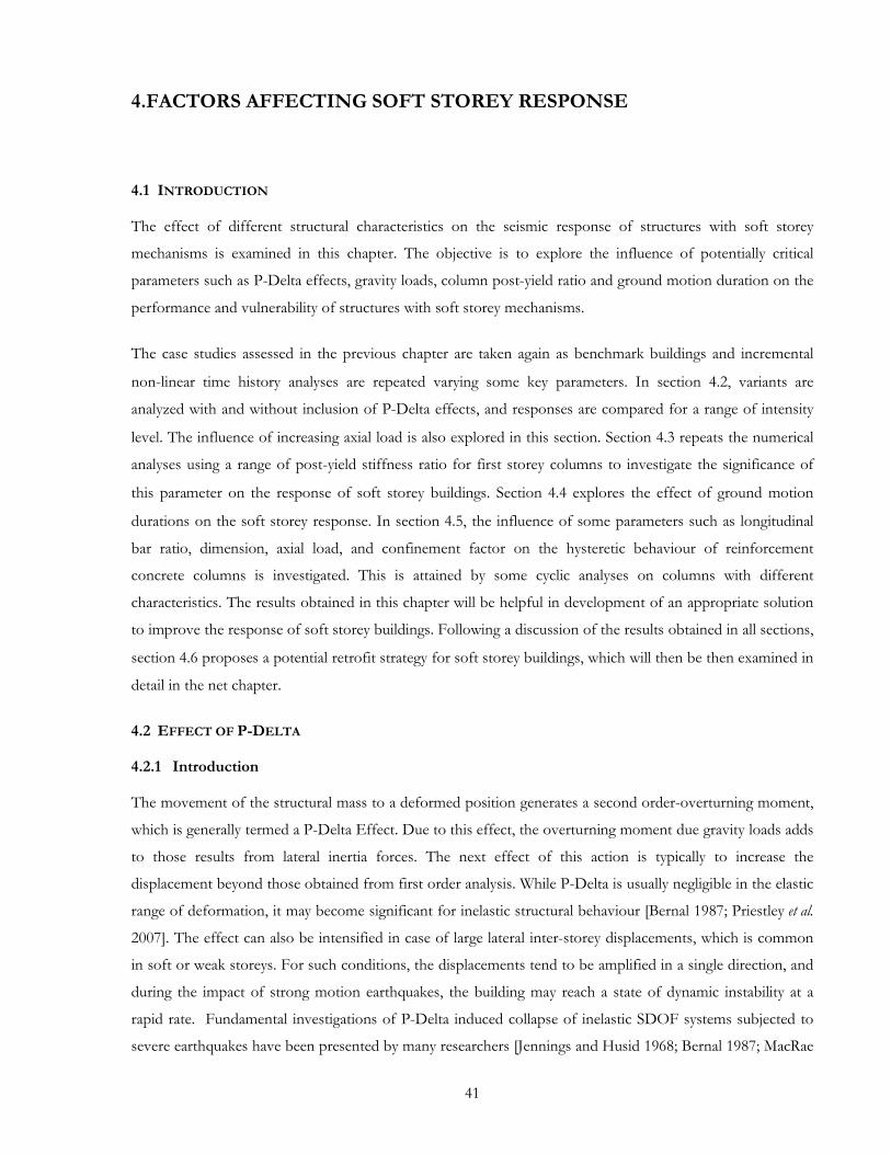
41
4.FACTORS AFFECTING SOFT STOREY RESPONSE
4.1 INTRODUCTION
The effect of different structural characteristics on the seismic response of structures with soft storey
mechanisms is examined in this chapter. The objective is to explore the influence of potentially critical
parameters such as P-Delta effects, gravity loads, column post-yield ratio and ground motion duration on the
performance and vulnerability of structures with soft storey mechanisms.
The case studies assessed in the previous chapter are taken again as benchmark buildings and incremental
non-linear time history analyses are repeated varying some key parameters. In section 4.2, variants are
analyzed with and without inclusion of P-Delta effects, and responses are compared for a range of intensity
level. The influence of increasing axial load is also explored in this section. Section 4.3 repeats the numerical
analyses using a range of post-yield stiffness ratio for first storey columns to investigate the significance of
this parameter on the response of soft storey buildings. Section 4.4 explores the effect of ground motion
durations on the soft storey response. In section 4.5, the influence of some parameters such as longitudinal
bar ratio, dimension, axial load, and confinement factor on the hysteretic behaviour of reinforcement
concrete columns is investigated. This is attained by some cyclic analyses on columns with different
characteristics. The results obtained in this chapter will be helpful in development of an appropriate solution
to improve the response of soft storey buildings. Following a discussion of the results obtained in all sections,
section 4.6 proposes a potential retrofit strategy for soft storey buildings, which will then be then examined in
detail in the net chapter.
4.2 EFFECT OF P-DELTA
4.2.1 Introduction
The movement of the structural mass to a deformed position generates a second order-overturning moment,
which is generally termed a P-Delta Effect. Due to this effect, the overturning moment due gravity loads adds
to those results from lateral inertia forces. The next effect of this action is typically to increase the
displacement beyond those obtained from first order analysis. While P-Delta is usually negligible in the elastic
range of deformation, it may become significant for inelastic structural behaviour [Bernal 1987; Priestley et al.
2007]. The effect can also be intensified in case of large lateral inter-storey displacements, which is common
in soft or weak storeys. For such conditions, the displacements tend to be amplified in a single direction, and
during the impact of strong motion earthquakes, the building may reach a state of dynamic instability at a
rapid rate. Fundamental investigations of P-Delta induced collapse of inelastic SDOF systems subjected to
severe earthquakes have been presented by many researchers [Jennings and Husid 1968; Bernal 1987; MacRae
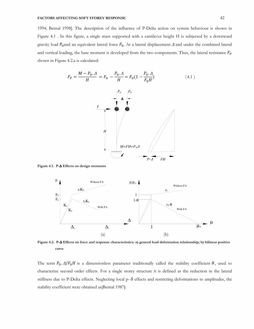
FACTORS AFFECTING SOFT STOREY RESPONSE 42
1994; Bernal 1998]. The description of the influence of P-Delta action on system behaviour is shown in
Figure 4.1 . In this figure, a single mass supported with a cantilever height H is subjected by a downward
gravity load ��and an equivalent lateral force O�. At a lateral displacement ∆ and under the combined lateral
and vertical loading, the base moment is developed from the two components. Thus, the lateral resistance O�
shown in Figure 4.2.a is calculated:
O� = � − ��.∆^ = O� − ��.∆^ = O�(1 − ��.∆O�^ ) ( 4.1 )
Figure 4.1. P-∆∆∆∆ Effects on design moments
(a) (b)
Figure 4.2. P-∆∆∆∆ Effects on force and response characteristics: a) general load deformation relationship; b) bilinear positive
curve
The term ��.∆/O�^ is a dimensionless parameter traditionally called the stability coefficient ' , used to
characterize second order effects. For a single storey structure it is defined as the reduction in the lateral
stiffness due to P-Delta effects. Neglecting local p- � effects and restricting deformations to amplitudes, the
stability coefficient were obtained as[Bernal 1987]:
H
P0
∆∆∆∆
P0
M=FH+P0 ∆
F
P-∆ FH
F 0
Without P∆
K0
r0 K0
F p
K p
F
∆
∆y ∆ u
1
Without P ∆
r0
1-θ
1
µµ m
rp Kp r0-θ
With P∆
F/F0
With P∆
FACTORS AFFECTING SOFT STOREY RESPONSE 43
'�∆ = �.∆O�^ = � �^ ( 4.2 )
where � is the first order initial lateral stiffness, and P is the total vertical load. Therefore, the reduced lateral
force capacity and stiffness shown in Figure 4.2.a was determined as
O� = O�(1 − '�∆) � = O�∆� = �(1 − '�∆) ( 4.3 )
The amount that the post-yield stiffness ratio is decreased as a function of the stability coefficient was found
as:
�� = �� − '�∆1 − '�∆ ( 4.4 )
Figure 4.2.b shows the influence of P-Delta effects on the normalized bilinear force displacement curve. For
an elasto-plastic system (r0 =0), the second order curve is defined by the first order results and '. The post
yield stiffness of a single-degree-of-freedom SDOF systems considering P-Delta effect KPP is calculated as
[Bernal 1987]
� = �� � = �� − '�∆1 − '�∆ �(1 − '�∆) = �� − '�∆ ( 4.5 )
The limit of ductility o� was found as:
o� − 1 = 1 − '�∆�� − '�∆ = 1�, → o� = 1 + 1�, ( 4.6 )
4.2.2 Effect of P-Delta on hysteretic response
The significance of P-Delta effects depends on the shape of the hysteretic response. If the earthquake record
is long enough, reduction of post-yield stiffness instability will eventually occur, which causes collapse.
[Priestley et al. 2007] This phenomenon more likely happens if an elasto-plastic curve is adopted for defining
hysteretic characteristics. The reason has been explained because unloading lines has a tendency to shift to the
right hand of the graph, which after several cycles, strength will be lost. Furthermore, considering P-Delta
effects can increase residual displacements. On the other hand, if Takeda hysteretic rule is considered, this
effect can be less important due to gradual reduction of residual displacement. [Priestley et al. 2007]
FACTORS AFFECTING SOFT STOREY RESPONSE 44
4.2.3 Design procedure for P-Delta effects
There are several design procedures and recommendations proposed by researchers when P-Delta effects are
considered. Among them a displacement amplification factor �,∆, the ratio between displacement spectra
with and without P-Delta effects, proposed by Bernal [1987] is outlined here. Based on this work, behaviour
of displacement amplification factors for linear and nonlinear SDOF systems were investigated. Bernal found
that the inelastic amplification was only weakly dependent on the period for a range of initial period from
zero to two seconds. In the course of his parametric study, the following expression for �,∆, which is only a
function of stability coefficient and the design ductility, was proposed as:
�,∆ = 1 + �,∆',∆1 − ',∆ ( 4.7 )
where �,∆ = 1.87(o − 1)for mean amplification and �,∆ = 2.69(o − 1) for mean+1 standard deviation
amplification. He also offered a limiting ductility o�, which should be considered for design:
o� = 0.4',∆ ( 4.8 )
This ductility limit was obtained based on the concept of ultimate stability under the permanently deformed
state of the structure following the earthquake and assuming that the post-earthquake permanent deformation
is the maximum value compatible with the response ductility.
In addition to the above consideration, a practical range of values for stability ratio was determined as follows
[Bernal 1998]:
',∆ = � �^ = �� �^ = ��� �^ = �'� ( 4.9 )
where � is the ratio of the total vertical load (dead load plus reduced live load) to the dead load, � is the inter-
storey drift ratio, and C is the code seismic coefficient.
4.2.4 Code recommendations
Most building design codes do not appear to give adequate guidance or advice on methods of counting for
and reducing P-Delta effects [Paulay and Priestley 1992]. In some instances [FEMA 1997]displacement
amplification factors are provided thus forcing implicit allowance for the modified response, rather than
explicit account for P-Delta behaviour. In the newer version [FEMA 356, 2000] all seismic forces and
displacements obtained from linear analysis approach are increased by the factor 1/(1 − ') when stability
coefficient of the first mode is more than 0.1. However, this limit could be inadequate unless the response is
elastic[Bernal 1987].
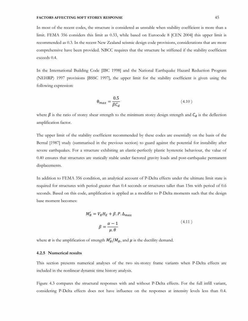
FACTORS AFFECTING SOFT STOREY RESPONSE 45
In most of the recent codes, the structure is considered as unstable when stability coefficient is more than a
limit. FEMA 356 considers this limit as 0.33, while based on Eurocode 8 [CEN 2004] this upper limit is
recommended as 0.3. In the recent New Zealand seismic design code provisions, considerations that are more
comprehensive have been provided. NBCC requires that the structure be stiffened if the stability coefficient
exceeds 0.4.
In the International Building Code [IBC 1998] and the National Earthquake Hazard Reduction Program
(NEHRP) 1997 provisions [BSSC 1997], the upper limit for the stability coefficient is given using the
following expression:
�� = 0.5��� ( 4.10 )
where � is the ratio of storey shear strength to the minimum storey design strength and �� is the deflection
amplification factor.
The upper limit of the stability coefficient recommended by these codes are essentially on the basis of the
Bernal [1987] study (summarised in the previous section) to guard against the potential for instability after
severe earthquakes. For a structure exhibiting an elastic-perfectly plastic hysteretic behaviour, the value of
0.40 ensures that structures are statically stable under factored gravity loads and post-earthquake permanent
displacements.
In addition to FEMA 356 condition, an analytical account of P-Delta effects under the ultimate limit state is
required for structures with period greater than 0.4 seconds or structures taller than 15m with period of 0.6
seconds. Based on this code, amplification is applied as a modifier to P-Delta moments such that the design
base moment becomes:
��? = ��^� + �. �. ���
� = � − 1o. ' ( 4.11 )
where � is the amplification of strength ��? /��, and o is the ductility demand.
4.2.5 Numerical results
This section presents numerical analyses of the two six-storey frame variants when P-Delta effects are
included in the nonlinear dynamic time history analysis.
Figure 4.3 compares the structural responses with and without P-Delta effects. For the full infill variant,
considering P-Delta effects does not have influence on the responses at intensity levels less than 0.4.
FACTORS AFFECTING SOFT STOREY RESPONSE 46
However, after this intensity level, both peak drift ratio and residual drift ratio amplifies in a rapid rate. This
amplification could be due to the failure of masonry infills at the second floor and forming soft storey
mechanism at this intensity level.
For the soft storey variant, the impact of P-Delta effects is significant in a broader range of intensity level.
The P-Delta amplification on the peak drift ratio can be seen after intensity level 0.25. The difference
between the system response with and without P-Delta effects is not significant at low levels of intensity, and
this is probably a reflection of the low stability indices for this structure. As the intensity increases, this
difference increases. The drift ratios for the SS variant at the hazard level 0.6g is less than 6.0%, while when
P-Delta are considered, this value exceeds 8.5%.
( a) ( b)
Figure 4.3. Comparison of IDA response with and without P-∆∆∆∆ effects: a) peak drift ratio, b) residual drift ratio
The effect of P-Delta on the residual drift is much more sensitive to the increasing level of intensity. It can be
seen that the residual drift at a PGA of 0.6g is less than 1% without P-Delta effects, while P-Delta effects
amplify this value by a factor of approximately 5.
4.2.6 Effect of Increased P-Delta Effects
The effect of increased P-Delta loads on the SS variant response is investigated in this section. This could be
expected for buildings with lateral load resisting frames in external bays and gravity frames internally, where
diaphragms are rigid and can transfer lateral loads from the middle spans to external ones. In this case,
vertical loads due to P-Delta effects are increased, while gravity loads on the columns are not changed. The
increasing of the P-Delta loads in critical conditions could easily be two times, where the P-Delta tributary
area in the external resisting frames is doubled.
Assuming this scenario, the nonlinear IDA was repeated when P-Delta loads are doubled. In order to
consider the effect of increasing the axial load related to P-Delta effects without changing the gravity load on
the case study column elements, dummy columns were added to the structure and extra vertical loads are
assigned to them (Figure 4.4).
0.050.10.150.20.250.30.350.4 0.60
2
4
6
8
10
Pe
ak d
rift r
atio
(%)
PGA(g)
0.050.10.150.20.250.30.350.4 0.60
1
2
3
4
5
6
Re
sid
ua
l d
rift r
atio
(%)
PGA(g)PGA(g)
FI-NPD SS-NPD FI SS

FACTORS AFFECTING SOFT STOREY RESPONSE 47
Figure 4.4. Dummy column modelling for considering effect of axial load
It should be noted that care is required in order to ensure that dummy columns do not add any stiffness to
the structure. For this reason, dummy columns are transversally slaved to a structural element at each level,
while other degrees of freedom (including end rotations) were released.
Results obtained for the SS variant where the total gravity load related to P-Delta effects is doubled (i.e. two
times the P-Delta coefficients, SS-DPD) are shown in Figure 4.5. In this case, the structure was unstable for
certain accelerograms at intensities greater than PGA=0.3g, with 90% of records causing dynamic instability
at a PGA=0.4g, and thus, the drift response is shown only up to an intensity level of 0.4g.
Figure 4.5. Comparison of responses obtained from incremental NTHA when the total gravity load is doubled
The results of this section indicate that vertical loads can have a significant effect on the response. The
incremental nonlinear time history analysis shows that for the case where the gravity load related to P-Delta
effects is doubled, the peak storey drifts at moderate levels of intensity and higher are more than two times
those for the case without P-Delta effects, and thus the potential collapse of the soft storey frame is
significantly increased. However, the increasing P-Delta effect on soft storey behaviour at low intensity levels
is not significant. As a result, it can be concluded that the importance of gravity load on the response of soft
storey buildings is highly affected by the intensity level, and the effect is increased as the intensity level is
Dummy
Column
0.05 0.1 0.15 0.2 0.25 0.3 0.35 0.40
5
10
15
20
Pea
k d
rift ra
tio
(%)
PGA(g)
SS-NPD
SS
SS-DPD
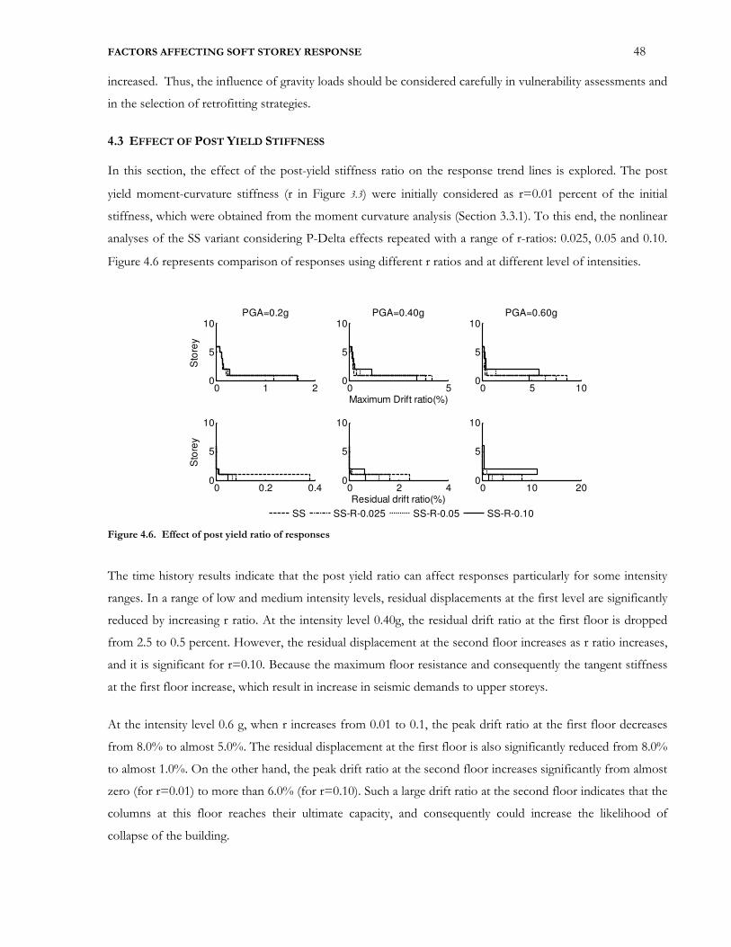
FACTORS AFFECTING SOFT STOREY RESPONSE 48
increased. Thus, the influence of gravity loads should be considered carefully in vulnerability assessments and
in the selection of retrofitting strategies.
4.3 EFFECT OF POST YIELD STIFFNESS
In this section, the effect of the post-yield stiffness ratio on the response trend lines is explored. The post
yield moment-curvature stiffness (r in Figure 3.3) were initially considered as r=0.01 percent of the initial
stiffness, which were obtained from the moment curvature analysis (Section 3.3.1). To this end, the nonlinear
analyses of the SS variant considering P-Delta effects repeated with a range of r-ratios: 0.025, 0.05 and 0.10.
Figure 4.6 represents comparison of responses using different r ratios and at different level of intensities.
Figure 4.6. Effect of post yield ratio of responses
The time history results indicate that the post yield ratio can affect responses particularly for some intensity
ranges. In a range of low and medium intensity levels, residual displacements at the first level are significantly
reduced by increasing r ratio. At the intensity level 0.40g, the residual drift ratio at the first floor is dropped
from 2.5 to 0.5 percent. However, the residual displacement at the second floor increases as r ratio increases,
and it is significant for r=0.10. Because the maximum floor resistance and consequently the tangent stiffness
at the first floor increase, which result in increase in seismic demands to upper storeys.
At the intensity level 0.6 g, when r increases from 0.01 to 0.1, the peak drift ratio at the first floor decreases
from 8.0% to almost 5.0%. The residual displacement at the first floor is also significantly reduced from 8.0%
to almost 1.0%. On the other hand, the peak drift ratio at the second floor increases significantly from almost
zero (for r=0.01) to more than 6.0% (for r=0.10). Such a large drift ratio at the second floor indicates that the
columns at this floor reaches their ultimate capacity, and consequently could increase the likelihood of
collapse of the building.
0 1 20
5
10PGA=0.2g
Sto
rey
0 0.2 0.40
5
10
Sto
rey
0 50
5
10PGA=0.40g
Maximum Drift ratio(%)
0 2 40
5
10
Residual drift ratio(%)
0 5 100
5
10PGA=0.60g
0 10 200
5
10
SS SS-R-0.025 SS-R-0.05 SS-R-0.10
FACTORS AFFECTING SOFT STOREY RESPONSE 49
As a conclusion, the potential advantage of increasing post yield drift ratio of columsn at the first level of soft
storey buildings could be reducing both peak and residual displacements at this single level. However, the
disadvantage is that they can increase seismic demands at the storeys above this floor. This strategy might not
be the best solution for retrofitting soft storey buildings because structural elements at the upper storeys
might be required to be strengthened, which could increase the retrofit cost.
4.4 EFFECT OF DURATION OF GROUND MOTION
The influence of strong-ground motion duration is the focus of this section. The importance of this effect is
due to the fact that the strong duration is closely related to the number of inelastic cycles that structural
elements suffer during earthquake excitation.
There are a number of studies related to effects of the strong-motion duration on the seismic response of
building structures. However, the findings regarding these effects are contradictory. Some studies report
significant effects, while other studies report minimal or no effects.
Hancock and Bommer [2006] observed that this controversy begins with response parameter used for the
quantification of the effects of strong-motion duration, and the definition of duration of strong ground
shaking of acceleration time histories recorded from earthquake events that adequately represent the time
interval when the energy content of the earthquake ground shaking produces significant damage to the
excited structure. Ruiz-Garcia [2010] concluded that strong motion duration does not have a significant
influence on the amplitude of peak residual drift demands in multi-degree-of-freedom MDOF systems, but
he pointed out that records having long strong-motion duration tend to increase residual drift demands in the
upper stories of long-period generic frames.
The following subsections investigate the effect of the strong-motion duration on the response of the
reinforced concrete frames with soft first storey (SS variant).
4.4.1 Selection of records
There are several definitions in the literature for determining the effective time duration of accelograms.
Among them, the most widely used measure of strong ground motion duration for earthquake engineering
purposes corresponds to the time interval over which 5% to 95% of the Arias intensity is transferred in the
acceleration time-history [Trifunac and Brady 1975]. The merit of this definition is that the use of Arias
Intensity has strong correlation with observed earthquake damages in short period structures as well as
structures on soils susceptible to liquefaction, but a limitation is that it does not explicitly take into account
differences in ground motion frequency-content as well as the source geophysical features [Bommer and
Martinez-Pereira 1999].
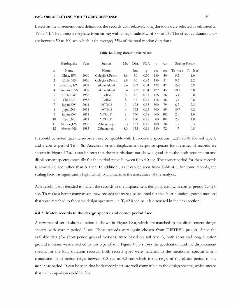
FACTORS AFFECTING SOFT STOREY RESPONSE 50
Based on the aforementioned definition, the records with relatively long duration were selected as tabulated in
Table 4.1. The motions originate from strong with a magnitude Mw of 8.0 to 9.0. The effective durations teff
are between 50 to 100 sec, which is (in average) 35% of the total motion duration t.
Table 4.1. Long duration record sets
It should be noted that the records were compatible with Eurocode 8 spectrum [CEN 2004] for soil type C
and a corner period Td = 8s. Acceleration and displacement response spectra for these set of records are
shown in Figure 4.7.a. It can be seen that the records does not show a good fit to the both acceleration and
displacement spectra especially for the period range between 0 to 4.0 sec. The corner period for these records
is almost 2.0 sec rather than 8.0 sec. In addition , as it can be seen from Table 4.1, for some records, the
scaling factor is significantly high, which could increase the inaccuracy of the analysis.
As a result, it was decided to match the records to the displacement design spectra with corner period Td=2.0
sec. To make a better comparison, new records set were also adopted for the short duration ground motions
that were matched to the same design spectrum, i.e. Td=2.0 sec, as it is discussed in the next section.
4.4.2 Match records to the design spectra and cornet period 2sec
A new record set of short duration is shown in Figure 4.8.a, which are matched to the displacement design
spectra with corner period 2 sec. These records were again chosen from DISTEEL project. Since the
available data (for short period ground motions) were based on soil type A, both short and long duration
ground motions were matched to this type of soil. Figure 4.8.b shows the acceleration and the displacement
spectra for the long duration records. Both record types were matched to the mentioned spectra with a
concentration of period range between 0.8 sec to 4.0 sec, which is the range of the elastic period to the
nonlinear period. It can be seen that both record sets, are well compatible to the design spectra, which means
that the comparison could be fare.
Earthquake Year Station Mw Dist. PGA t teff Scaling Factor
# Name
Name
km g sec sec Td=4sec Td=2sec
1 Chile, EW 2010 Colegio S.Pedro 8.8 30 0.70 180 50 5.2 1.0
2 Chile, NS 2010 Colegio S.Pedro 8.8 30 0.93 180 51 9.6 2.2
3 Sumatra, EW 2007 Sikuai Island 8.4 392 0.04 129 47 15.6 6.9
4 Sumatra, NS 2007 Sikuai Island 8.4 392 0.04 129 45 18.3 6.8
5 Chile,EW 1985 Llolleo 8 42 0.71 116 36 3.4 0.8
6 Chile,NS 1985 Llolleo 8 42 0.71 116 36 3.4 0.8
7 Japan,EW 2011 IWT008 9 123 0.33 300 79 6.7 2.3
8 Japan,NS 2011 IWT008 9 123 0.25 300 69 10.7 4.2
9 Japan,EW 2011 MYG011 9 170 0.68 300 105 2.9 1.0
10 Japan,NS 2011 MYG011 9 170 0.92 300 104 2.7 1.8
11 Mexico,EW 1985 Zihuatanejo 8.3 133 0.17 180 38 1.7 0.3
12 Mexico,NS 1985 Zihuatanejo 8.3 133 0.11 180 72 1.7 0.5
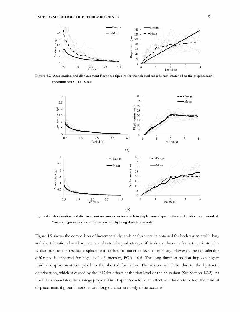
FACTORS AFFECTING SOFT STOREY RESPONSE 51
Figure 4.7. Acceleration and displacement Response Spectra for the selected records sets: matched to the displacement
spectrum soil C, Td=8.sec
(a)
(b)
Figure 4.8. Acceleration and displacement response spectra match to displacement spectra for soil A with corner period of
2sec soil type A: a) Short duration records b) Long duration records
Figure 4.9 shows the comparison of incremental dynamic analysis results obtained for both variants with long
and short durations based on new record sets. The peak storey drift is almost the same for both variants. This
is also true for the residual displacement for low to moderate level of intensity. However, the considerable
difference is appeared for high level of intensity, PGA =0.6. The long duration motion imposes higher
residual displacement compared to the short deformation. The reason would be due to the hysteretic
deterioration, which is caused by the P-Delta effects at the first level of the SS variant (See Section 4.2.2). As
it will be shown later, the strategy proposed in Chapter 5 could be an effective solution to reduce the residual
displacements if ground motions with long duration are likely to be occurred.
0
0.5
1
1.5
2
2.5
3
0.5 1.5 2.5 3.5 4.5
Acc
eler
atio
n (
g)
Period (s)
Design
Mean
0
20
40
60
80
100
120
140
0 2 4 6 8
Dis
pla
cem
ent
(cm
)
Period (s)
Design
Mean
0
0.5
1
1.5
2
2.5
3
0.5 1.5 2.5 3.5 4.5
Acc
eler
atio
n (
g)
Period (s)
0
5
10
15
20
25
30
35
40
0 1 2 3 4
Dis
pla
cem
ent
(cm
)
Period (s)
Design
Mean
0
0.5
1
1.5
2
2.5
3
0.5 1.5 2.5 3.5 4.5
Acc
eler
atio
n (
g)
Period (s)
Design
Mean
0
5
10
15
20
25
30
35
40
0 1 2 3 4
Dis
pla
cem
ent
(cm
)
Period (s)
Design
Mean
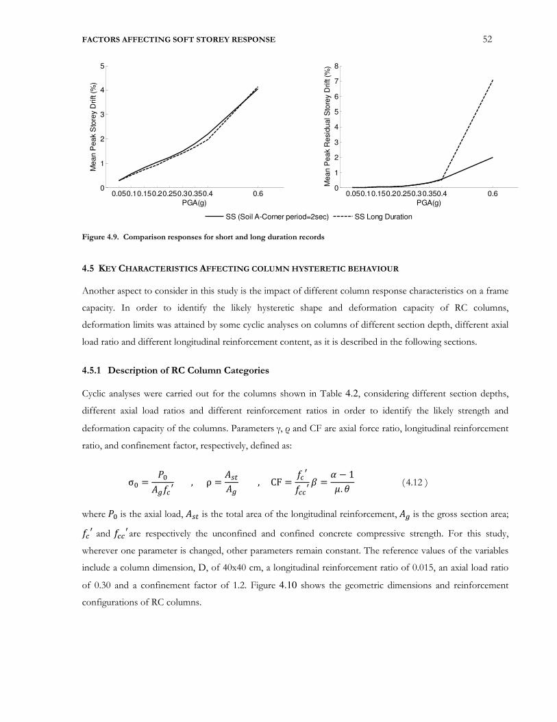
FACTORS AFFECTING SOFT STOREY RESPONSE 52
Figure 4.9. Comparison responses for short and long duration records
4.5 KEY CHARACTERISTICS AFFECTING COLUMN HYSTERETIC BEHAVIOUR
Another aspect to consider in this study is the impact of different column response characteristics on a frame
capacity. In order to identify the likely hysteretic shape and deformation capacity of RC columns,
deformation limits was attained by some cyclic analyses on columns of different section depth, different axial
load ratio and different longitudinal reinforcement content, as it is described in the following sections.
4.5.1 Description of RC Column Categories
Cyclic analyses were carried out for the columns shown in Table 4.2, considering different section depths,
different axial load ratios and different reinforcement ratios in order to identify the likely strength and
deformation capacity of the columns. Parameters γ, ρ and CF are axial force ratio, longitudinal reinforcement
ratio, and confinement factor, respectively, defined as:
σ� = ��X|F*? , ρ = Xp�X| , CF = F*?F**? � = � − 1o. ' ( 4.12 )
where �� is the axial load, Xp� is the total area of the longitudinal reinforcement, X| is the gross section area;
F*? and F**?are respectively the unconfined and confined concrete compressive strength. For this study,
wherever one parameter is changed, other parameters remain constant. The reference values of the variables
include a column dimension, D, of 40x40 cm, a longitudinal reinforcement ratio of 0.015, an axial load ratio
of 0.30 and a confinement factor of 1.2. Figure 4.10 shows the geometric dimensions and reinforcement
configurations of RC columns.
0.050.10.150.20.250.30.350.4 0.60
1
2
3
4
5
Mean P
eak S
tore
y D
rift (%
)
PGA(g)
0.050.10.150.20.250.30.350.4 0.60
1
2
3
4
5
6
7
8
Mean P
eak R
esid
ual S
tore
y D
rift (%
)
PGA(g)
SS (Soil A-Corner period=2sec) SS Long Duration

FACTORS AFFECTING SOFT STOREY RESPONSE 53
Table 4.2. Characteristics of different column studied, with a cantilever length of 3m
Var. Case Depth Width ¡ σ� CF
m m
Var
iant I
1 0.4 0.4 0.0025 0.3 1.2
2 0.4 0.4 0.005 0.3 1.2
3 0.4 0.4 0.01 0.3 1.2
4 0.4 0.4 0.015 0.3 1.2
5 0.4 0.4 0.02 0.3 1.2
6 0.4 0.4 0.03 0.3 1.2
7 0.4 0.4 0.035 0.3 1.2
8 0.4 0.4 0.04 0.3 1.2
Var
iant II
1 0.25 0.25 0.015 0.3 1.2
2 0.3 0.3 0.015 0.3 1.2
3 0.35 0.35 0.015 0.3 1.2
4 0.40 0.40 0.015 0.3 1.2
5 0.50 0.50 0.015 0.3 1.2
Var
iant II
I
1 0.4 0.4 0.015 -0.05 1.2
2 0.4 0.4 0.015 0 1.2
3 0.4 0.4 0.015 0.05 1.2
4 0.4 0.4 0.015 0.1 1.2
5 0.4 0.4 0.015 0.2 1.2
6 0.4 0.4 0.015 0.3 1.2
7 0.4 0.4 0.015 0.4 1.2
8 0.4 0.4 0.015 0.5 1.2
Var
iant IV
1 0.4 0.4 0.015 0.3 1
2 0.4 0.4 0.015 0.3 1.05
3 0.4 0.4 0.015 0.3 1.1
4 0.4 0.4 0.015 0.3 1.2
5 0.4 0.4 0.015 0.3 1.4
6 0.4 0.4 0.015 0.3 1.6
7 0.4 0.4 0.015 0.3 1.8
8 0.4 0.4 0.015 0.3 2
FACTORS AFFECTING SOFT STOREY RESPONSE 54
Figure 4.10. Different configuration of steel reinforcement and column size of the RC concrete columns
4.5.2 Description of numerical modelling
Numerical models were developed and analyzed in Seismo-Struct [SeismoSoft 2004] for all geometrical and
loading characteristics. All 3.00m high piers were modelled by three force-based elements along the column
height, the bottom one having 0.50m.
Five integration sections per element were used, each one containing 200 integration points. In order to
account for the cyclic degradation of steel strength depicted by the experimental results without changing the
steel model, a negative value of the parameter a3 was considered. The steel Young’s modulus was taken equal
to 200 GPa. The hardening and cyclic behaviour parameters were calibrated in order to better reproduce past
experimental results (see next section): b = 0.015, R0 = 20, a1 = 18.5, a2 = 0.15, a3 = -0.025 and a4 =15.
The model of Filippou et al. [1983] was applied for the longitudinal reinforcement. The steel Young’s
modulus was taken equal to 200 GPa. The iterative procedure developed by Taucer et al. [1991] and Spacone
et al. [1996] was adopted for the force-based element. Additionally, a co-rotational formulation was used to
account for geometrical nonlinear effects.
The force or flexibility-based formulation was used for defining the nonlinear fibre element. Force-based
elements satisfy exactly the equilibrium conditions by using an exact description for the stress resultants’ field
throughout the frame element length. On the other hand, in displacement based elements an approximation
is made for the displacement field throughout the frame element length, from which strains, stresses and
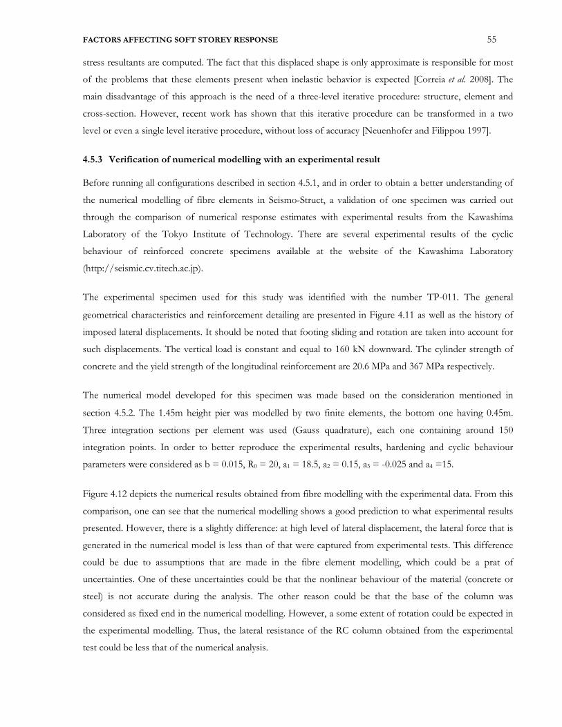
FACTORS AFFECTING SOFT STOREY RESPONSE 55
stress resultants are computed. The fact that this displaced shape is only approximate is responsible for most
of the problems that these elements present when inelastic behavior is expected [Correia et al. 2008]. The
main disadvantage of this approach is the need of a three-level iterative procedure: structure, element and
cross-section. However, recent work has shown that this iterative procedure can be transformed in a two
level or even a single level iterative procedure, without loss of accuracy [Neuenhofer and Filippou 1997].
4.5.3 Verification of numerical modelling with an experimental result
Before running all configurations described in section 4.5.1, and in order to obtain a better understanding of
the numerical modelling of fibre elements in Seismo-Struct, a validation of one specimen was carried out
through the comparison of numerical response estimates with experimental results from the Kawashima
Laboratory of the Tokyo Institute of Technology. There are several experimental results of the cyclic
behaviour of reinforced concrete specimens available at the website of the Kawashima Laboratory
(http://seismic.cv.titech.ac.jp).
The experimental specimen used for this study was identified with the number TP-011. The general
geometrical characteristics and reinforcement detailing are presented in Figure 4.11 as well as the history of
imposed lateral displacements. It should be noted that footing sliding and rotation are taken into account for
such displacements. The vertical load is constant and equal to 160 kN downward. The cylinder strength of
concrete and the yield strength of the longitudinal reinforcement are 20.6 MPa and 367 MPa respectively.
The numerical model developed for this specimen was made based on the consideration mentioned in
section 4.5.2. The 1.45m height pier was modelled by two finite elements, the bottom one having 0.45m.
Three integration sections per element was used (Gauss quadrature), each one containing around 150
integration points. In order to better reproduce the experimental results, hardening and cyclic behaviour
parameters were considered as b = 0.015, R0 = 20, a1 = 18.5, a2 = 0.15, a3 = -0.025 and a4 =15.
Figure 4.12 depicts the numerical results obtained from fibre modelling with the experimental data. From this
comparison, one can see that the numerical modelling shows a good prediction to what experimental results
presented. However, there is a slightly difference: at high level of lateral displacement, the lateral force that is
generated in the numerical model is less than of that were captured from experimental tests. This difference
could be due to assumptions that are made in the fibre element modelling, which could be a prat of
uncertainties. One of these uncertainties could be that the nonlinear behaviour of the material (concrete or
steel) is not accurate during the analysis. The other reason could be that the base of the column was
considered as fixed end in the numerical modelling. However, a some extent of rotation could be expected in
the experimental modelling. Thus, the lateral resistance of the RC column obtained from the experimental
test could be less that of the numerical analysis.

FACTORS AFFECTING SOFT STOREY RESPONSE 56
Figure 4.11. Geometrical characteristics of the specimen and history of cyclic loading
-100
-50
0
50
100
0 1 2 3 4 5 6 7 8 9 10 11 12
Displacement (m
m)
Cycle
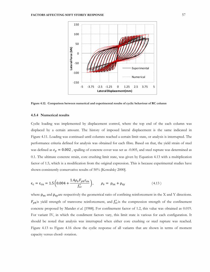
FACTORS AFFECTING SOFT STOREY RESPONSE 57
Figure 4.12. Comparison between numerical and experimental results of cyclic behaviour of RC column
4.5.4 Numerical results
Cyclic loading was implemented by displacement control, where the top end of the each column was
displaced by a certain amount. The history of imposed lateral displacement is the same indicated in
Figure 4.11. Loading was continued until columns reached a certain limit state, or analysis is interrupted. The
performance criteria defined for analysis was obtained for each fibre. Based on that, the yield strain of steel
was defined as ¢£ = 0.002 , spalling of concrete cover was set as -0.005, and steel rupture was determined as
0.1. The ultimate concrete strain, core crushing limit state, was given by Equation 4.13 with a multiplication
factor of 1.5, which is a modification from the original expression. This is because experimental studies have
shown consistently conservative results of 50% [Kowalsky 2000].
ϵ/ = ε/= = 1.5 \0.004 + 1.4¡HO£¦¢pGF**? ` , ¡H = ρ>§ + ρ>¨ ( 4.13 )
where ρ>§ and ρ>¨are respectively the geometrical ratio of confining reinforcement in the X and Y directions.
O£¦ is yield strength of transverse reinforcement, and F**? is the compression strength of the confinement
concrete proposed by Mander et al. [1988]. For confinement factor of 1.2, this value was obtained as 0.019.
For variant IV, in which the condiment factors vary, this limit state is various for each configuration. It
should be noted that analysis was interrupted when either core crushing or steel rupture was reached.
Figure 4.13 to Figure 4.16 show the cyclic response of all variants that are shown in terms of moment
capacity versus chord- rotation.
-150
-100
-50
0
50
100
150
-5 -3.75 -2.5 -1.25 0 1.25 2.5 3.75 5
La
tera
l Fo
rce
(k
N)
Lateral Displacement(mm)
Experimental
Numerical
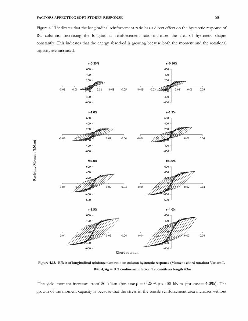
FACTORS AFFECTING SOFT STOREY RESPONSE 58
Figure 4.13 indicates that the longitudinal reinforcement ratio has a direct effect on the hysteretic response of
RC columns. Increasing the longitudinal reinforcement ratio increases the area of hysteretic shapes
constantly. This indicates that the energy absorbed is growing because both the moment and the rotational
capacity are increased.
Figure 4.13. Effect of longitudinal reinforcement ratio on column hysteretic response (Moment-chord rotation) Variant I,
©=0.4, AP = P. ª confinement factor: 1.2, cantilever length =3m
The yield moment increases from180 kN.m (for case ρ = 0.25% )to 400 kN.m (for case= 4.0%). The
growth of the moment capacity is because that the stress in the tensile reinforcement area increases without
-600
-400
-200
0
200
400
600
-0.05 -0.03 -0.01 0.01 0.03 0.05
r=0.25%
-600
-400
-200
0
200
400
600
-0.04 -0.02 0 0.02 0.04
r=1.0%
-600
-400
-200
0
200
400
600
-0.04 -0.02 0 0.02 0.04
r=2.0%
-600
-400
-200
0
200
400
600
-0.04 -0.02 0 0.02 0.04
r=3.5%
-600
-400
-200
0
200
400
600
-0.05 -0.03 -0.01 0.01 0.03 0.05
r=0.50%
-600
-400
-200
0
200
400
600
-0.04 -0.02 0 0.02 0.04
r=1.5%
-600
-400
-200
0
200
400
600
-0.04 -0.02 0 0.02 0.04
r=3.0%
-600
-400
-200
0
200
400
600
-0.04 -0.02 0 0.02 0.04
r=4.0%
Chord rotation
Resisting M
oment (kN.m
)
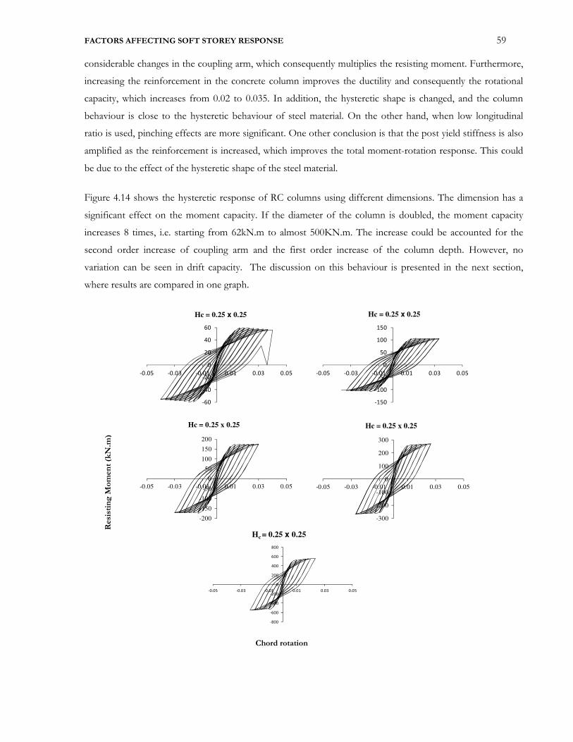
FACTORS AFFECTING SOFT STOREY RESPONSE 59
considerable changes in the coupling arm, which consequently multiplies the resisting moment. Furthermore,
increasing the reinforcement in the concrete column improves the ductility and consequently the rotational
capacity, which increases from 0.02 to 0.035. In addition, the hysteretic shape is changed, and the column
behaviour is close to the hysteretic behaviour of steel material. On the other hand, when low longitudinal
ratio is used, pinching effects are more significant. One other conclusion is that the post yield stiffness is also
amplified as the reinforcement is increased, which improves the total moment-rotation response. This could
be due to the effect of the hysteretic shape of the steel material.
Figure 4.14 shows the hysteretic response of RC columns using different dimensions. The dimension has a
significant effect on the moment capacity. If the diameter of the column is doubled, the moment capacity
increases 8 times, i.e. starting from 62kN.m to almost 500KN.m. The increase could be accounted for the
second order increase of coupling arm and the first order increase of the column depth. However, no
variation can be seen in drift capacity. The discussion on this behaviour is presented in the next section,
where results are compared in one graph.
-60
-40
-20
0
20
40
60
-0.05 -0.03 -0.01 0.01 0.03 0.05
Hc = 0.25 x 0.25
-300
-200
-100
0
100
200
300
-0.05 -0.03 -0.01 0.01 0.03 0.05
Hc = 0.25 x 0.25
-150
-100
-50
0
50
100
150
-0.05 -0.03 -0.01 0.01 0.03 0.05
Hc = 0.25 x 0.25
-200
-150
-100
-50
0
50
100
150
200
-0.05 -0.03 -0.01 0.01 0.03 0.05
Hc = 0.25 x 0.25
-800
-600
-400
-200
0
200
400
600
800
-0.05 -0.03 -0.01 0.01 0.03 0.05
Hc = 0.25 x 0.25
Resisting M
oment (kN.m
)
Chord rotation
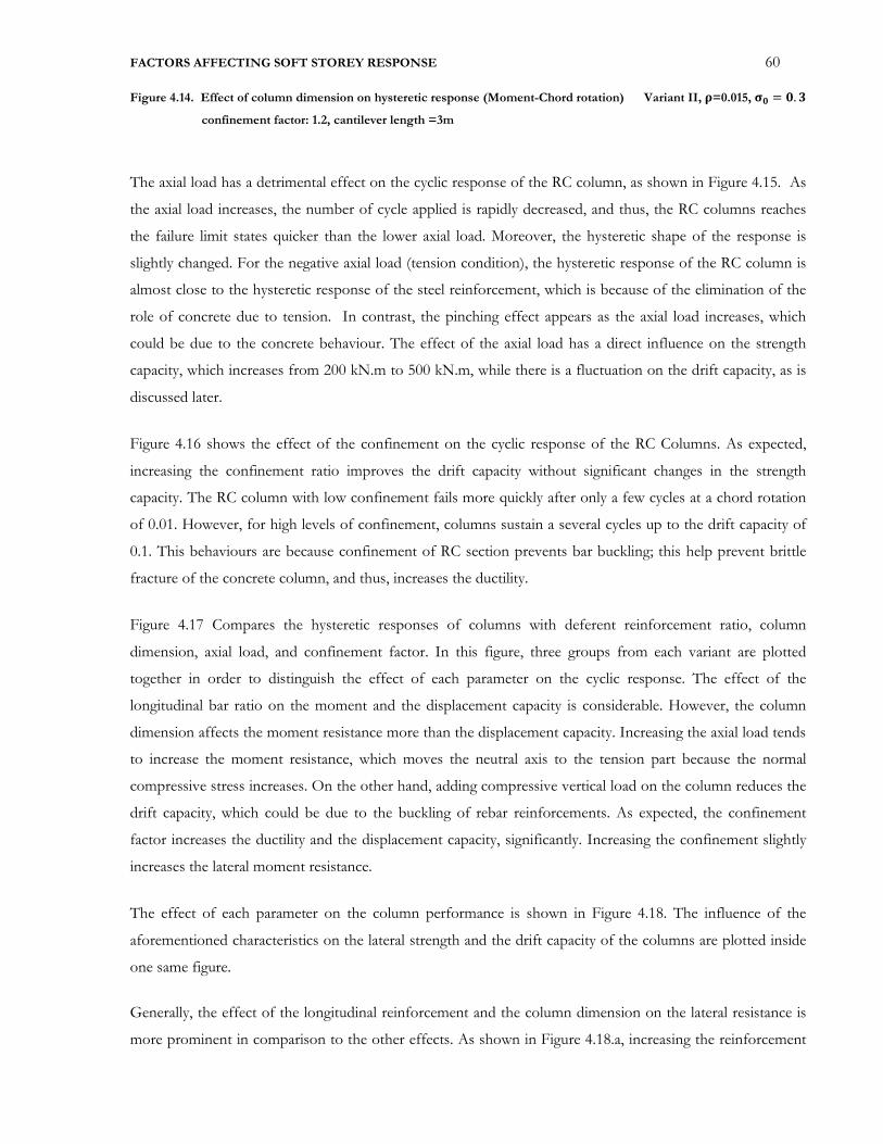
FACTORS AFFECTING SOFT STOREY RESPONSE 60
Figure 4.14. Effect of column dimension on hysteretic response (Moment-Chord rotation) Variant II, ¬=0.015, AP = P. ª confinement factor: 1.2, cantilever length =3m
The axial load has a detrimental effect on the cyclic response of the RC column, as shown in Figure 4.15. As
the axial load increases, the number of cycle applied is rapidly decreased, and thus, the RC columns reaches
the failure limit states quicker than the lower axial load. Moreover, the hysteretic shape of the response is
slightly changed. For the negative axial load (tension condition), the hysteretic response of the RC column is
almost close to the hysteretic response of the steel reinforcement, which is because of the elimination of the
role of concrete due to tension. In contrast, the pinching effect appears as the axial load increases, which
could be due to the concrete behaviour. The effect of the axial load has a direct influence on the strength
capacity, which increases from 200 kN.m to 500 kN.m, while there is a fluctuation on the drift capacity, as is
discussed later.
Figure 4.16 shows the effect of the confinement on the cyclic response of the RC Columns. As expected,
increasing the confinement ratio improves the drift capacity without significant changes in the strength
capacity. The RC column with low confinement fails more quickly after only a few cycles at a chord rotation
of 0.01. However, for high levels of confinement, columns sustain a several cycles up to the drift capacity of
0.1. This behaviours are because confinement of RC section prevents bar buckling; this help prevent brittle
fracture of the concrete column, and thus, increases the ductility.
Figure 4.17 Compares the hysteretic responses of columns with deferent reinforcement ratio, column
dimension, axial load, and confinement factor. In this figure, three groups from each variant are plotted
together in order to distinguish the effect of each parameter on the cyclic response. The effect of the
longitudinal bar ratio on the moment and the displacement capacity is considerable. However, the column
dimension affects the moment resistance more than the displacement capacity. Increasing the axial load tends
to increase the moment resistance, which moves the neutral axis to the tension part because the normal
compressive stress increases. On the other hand, adding compressive vertical load on the column reduces the
drift capacity, which could be due to the buckling of rebar reinforcements. As expected, the confinement
factor increases the ductility and the displacement capacity, significantly. Increasing the confinement slightly
increases the lateral moment resistance.
The effect of each parameter on the column performance is shown in Figure 4.18. The influence of the
aforementioned characteristics on the lateral strength and the drift capacity of the columns are plotted inside
one same figure.
Generally, the effect of the longitudinal reinforcement and the column dimension on the lateral resistance is
more prominent in comparison to the other effects. As shown in Figure 4.18.a, increasing the reinforcement
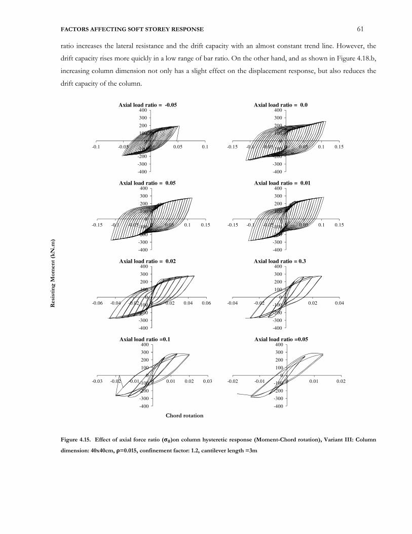
FACTORS AFFECTING SOFT STOREY RESPONSE 61
Chord rotation
ratio increases the lateral resistance and the drift capacity with an almost constant trend line. However, the
drift capacity rises more quickly in a low range of bar ratio. On the other hand, and as shown in Figure 4.18.b,
increasing column dimension not only has a slight effect on the displacement response, but also reduces the
drift capacity of the column.
Figure 4.15. Effect of axial force ratio (AP)on column hysteretic response (Moment-Chord rotation), Variant III: Column
dimension: 40x40cm, ¬=0.015, confinement factor: 1.2, cantilever length =3m
-400
-300
-200
-100
0
100
200
300
400
-0.15 -0.1 -0.05 0 0.05 0.1 0.15
Axial load ratio = 0.05
-400
-300
-200
-100
0
100
200
300
400
-0.15 -0.1 -0.05 0 0.05 0.1 0.15
Axial load ratio = 0.01
-400
-300
-200
-100
0
100
200
300
400
-0.1 -0.05 0 0.05 0.1
Axial load ratio = -0.05
-400
-300
-200
-100
0
100
200
300
400
-0.15 -0.1 -0.05 0 0.05 0.1 0.15
Axial load ratio = 0.0
-400
-300
-200
-100
0
100
200
300
400
-0.06 -0.04 -0.02 0 0.02 0.04 0.06
Axial load ratio = 0.02
-400
-300
-200
-100
0
100
200
300
400
-0.04 -0.02 0 0.02 0.04
Axial load ratio = 0.3
-400
-300
-200
-100
0
100
200
300
400
-0.03 -0.02 -0.01 0 0.01 0.02 0.03
Axial load ratio =0.1
-400
-300
-200
-100
0
100
200
300
400
-0.02 -0.01 0 0.01 0.02
Axial load ratio =0.05
Resisting M
oment (kN.m
)
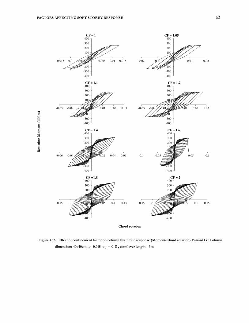
FACTORS AFFECTING SOFT STOREY RESPONSE 62
Chord rotation
Figure 4.16. Effect of confinement factor on column hysteretic response (Moment-Chord rotation) Variant IV: Column
dimension: 40x40cm, ¬=0.015 AP = P. ª , cantilever length =3m
-400
-300
-200
-100
0
100
200
300
400
-0.015 -0.01 -0.005 0 0.005 0.01 0.015
CF = 1
-400
-300
-200
-100
0
100
200
300
400
-0.02 -0.01 0 0.01 0.02
CF = 1.05
-400
-300
-200
-100
0
100
200
300
400
-0.03 -0.02 -0.01 0 0.01 0.02 0.03
CF = 1.1
-400
-300
-200
-100
0
100
200
300
400
-0.03 -0.02 -0.01 0 0.01 0.02 0.03
CF = 1.2
-400
-300
-200
-100
0
100
200
300
400
-0.06 -0.04 -0.02 0 0.02 0.04 0.06
CF = 1.4
-400
-300
-200
-100
0
100
200
300
400
-0.1 -0.05 0 0.05 0.1
CF = 1.6
-400
-300
-200
-100
0
100
200
300
400
-0.15 -0.1 -0.05 0 0.05 0.1 0.15
CF =1.8
-400
-300
-200
-100
0
100
200
300
400
-0.15 -0.1 -0.05 0 0.05 0.1 0.15
CF = 2
Resisting M
oment (kN.m
)

FACTORS AFFECTING SOFT STOREY RESPONSE 63
Figure 4.17. Comparison of key characteristics on the cyclic behaviour of RC columns
(a) ( b)
(c) ( d)
Figure 4.18. Effect of key characteristics on the hysteretic response of RC columns
Figure 4.18.c shows the effect of the axial load on the drift capacity and the lateral resistance of the RC
column. By increasing the axial load, the moment capacity of the column increases a certain amount and then
reduces. This is attributed to the classic axial load-bending moment interaction, whereby the most resistance
-600
-400
-200
0
200
400
600
-0.06 -0.04 -0.02 0 0.02 0.04
Mo
mn
et (k
N.m
)
Chord rotation
Varient 1
ρ=4.0%ρ=1.5%ρ=0.5% -800
-600
-400
-200
0
200
400
600
800
-0.04 -0.02 0 0.02 0.04
Mo
mn
et (k
N.m
)
Chord rotation
Varient 2
Hc=0.5x0.5
Hc=0.35x0.35
-400
-300
-200
-100
0
100
200
300
400
-0.06 -0.04 -0.02 0 0.02 0.04 0.06
Mo
mn
et (k
N.m
)
Chord rotation
Varient 3
σ0 = −0.05σ0 = −0.5σ0=−0.20 -400
-300
-200
-100
0
100
200
300
400
-0.15 -0.1 -0.05 0 0.05 0.1 0.15
Mo
mn
et (k
N.m
)
Chord rotation
Varient 4
CF = 1.2CF = 2
CF = 1
0.0
0.5
1.0
1.5
2.0
2.5
3.0
3.5
4.0
0
20
40
60
80
100
120
140
160
180
200
0.000 0.020 0.040 0.060
Sto
rey
dri
ft c
ap
aci
ty (%
)
La
tera
l Res
ista
nce
(k
N)
Longitudinal reinforcement ratio
Lateral reistance
Drift capacity0.0
0.5
1.0
1.5
2.0
2.5
3.0
3.5
4.0
4.5
0
20
40
60
80
100
120
140
160
180
200
0.20 0.40 0.60
Sto
rey
dri
ft c
ap
aci
ty (%
)
La
tera
l Res
ista
nce
(kN
)
Column Dimension (m)
Lateral reistance
Drift capacity
0.0
2.0
4.0
6.0
8.0
10.0
12.0
0
20
40
60
80
100
120
-0.1 0.2 0.4 0.6
Sto
rey
dri
ft c
ap
aci
ty (%
)
late
ral r
esis
tan
ce(k
N)
Axial load ratio
Lateral reistance
Drift capacity
0.0
2.0
4.0
6.0
8.0
10.0
12.0
0
20
40
60
80
100
120
140
1.00 1.50 2.00
Sto
rey
dri
ft c
ap
aci
ty (%
)
late
ral r
esis
tan
ce (
kN
)
Confinemnet Factor
Lateral reistance
Drift capacity

FACTORS AFFECTING SOFT STOREY RESPONSE 64
is achieved when deformation limits for the concrete and the reinforcement are obtained at the same time, i.e.
balance condition.
The results shown in Figure 4.18.d indicate that confinement has a significant influence on the drift capacity
up to a certain level, but doesn’t affect the strength significantly. This also agrees with traditional structural
mechanics considerations (see, for example, Paulay and Priestley [1992]). Some further discussion of the trend
lines and their implications for retrofit is provided at the end of this chapter.
4.5.5 Comparison of cyclic analysis with the section analysis
In this section, all variants are investigated again with section analysis and the results are compared to those
obtained based on fibre modelling from static time historey analysis. To this end, a detailed moment-
curvature analysis is conducted for all variants described in the previous section, and the effect of each
characteristic is investigated on the response.
Two concrete material models were used in the analysis; unconfined concrete for the cover and confined
concrete for the core of the section where lateral reinforcement surrounds the concrete. The same model of
Mander et al. [1988] was used as the constitutive relation for concrete in compression. For what concerns the
constitutive relations for reinforcement steel, the model of King et al. [1986] is adopted.
In deriving the expressions of the moments and curvatures for the confinement concrete section, the
following classical assumptions were made:
• The strain profile is linear at all stages of loading up to failure.
• The stress-strain relationship is taken as a stress block, and the idealised stress-strain relation for the
tension and compression steel is used
• The tensile strength of concrete is neglected.
• The steel is perfectly bonded.
• Axial force is applied in the section centroid.
For obtaining the complete moment–curvature relationship for any cross-section, discrete values of concrete
strains (εc) were selected such that an even distribution of points on the plot were obtained, both before and
after the maximum. The procedure used to obtained moment-curvature is in accordance with the following
steps:
i) After dividing the section in to number of slices, the area of cover, core, and reinforcing steel in each
layer is determined.
ii) The strain of the extreme fibre (εc in
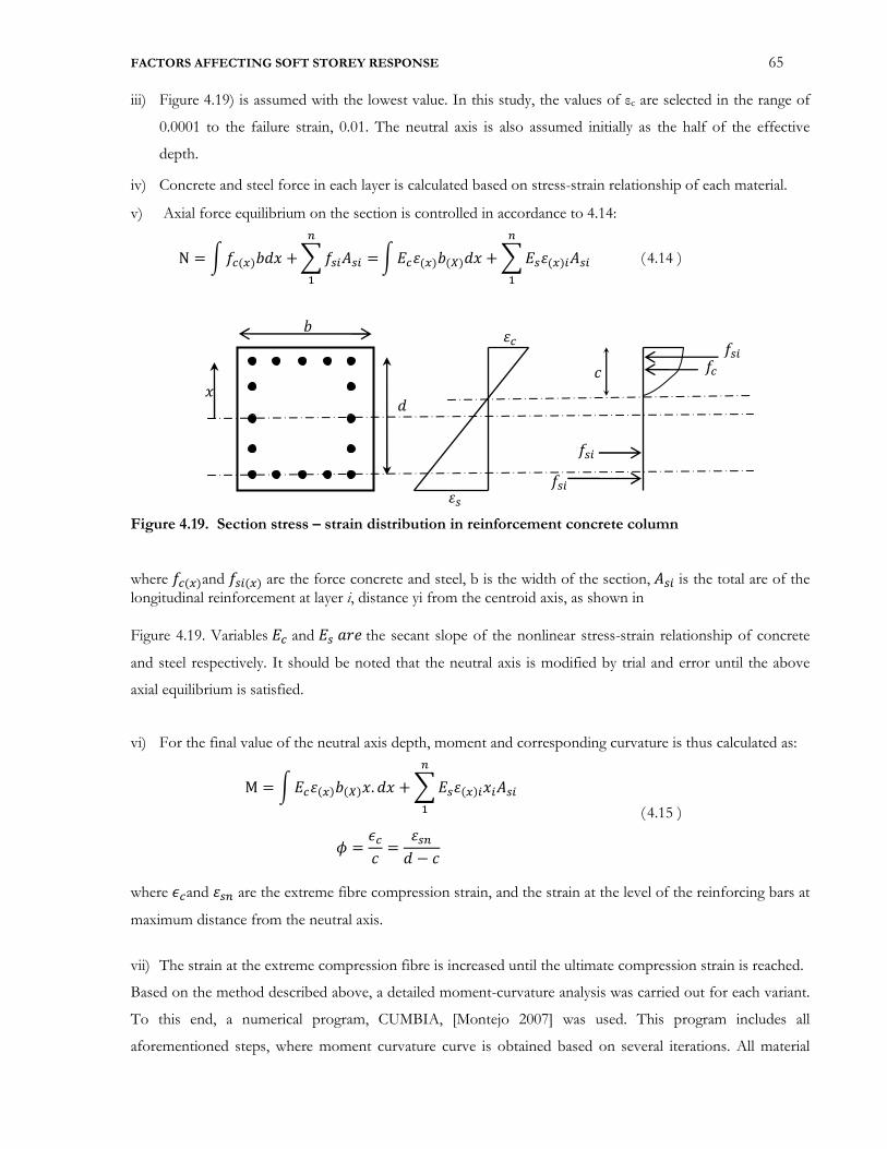
FACTORS AFFECTING SOFT STOREY RESPONSE 65
iii) Figure 4.19) is assumed with the lowest value. In this study, the values of εc are selected in the range of
0.0001 to the failure strain, 0.01. The neutral axis is also assumed initially as the half of the effective
depth.
iv) Concrete and steel force in each layer is calculated based on stress-strain relationship of each material.
v) Axial force equilibrium on the section is controlled in accordance to 4.14:
N = ® F*(�)��¯ + ° Fp�Xp� =±�
® *¢(�)�(²)�¯ + ° p¢(�)�Xp�±�
( 4.14 )
Figure 4.19. Section stress – strain distribution in reinforcement concrete column
where F*(�)and Fp�(�) are the force concrete and steel, b is the width of the section, Xp� is the total are of the longitudinal reinforcement at layer i, distance yi from the centroid axis, as shown in
Figure 4.19. Variables * and p ³�´ the secant slope of the nonlinear stress-strain relationship of concrete
and steel respectively. It should be noted that the neutral axis is modified by trial and error until the above
axial equilibrium is satisfied.
vi) For the final value of the neutral axis depth, moment and corresponding curvature is thus calculated as:
M = ® *¢(�)�(²)¯. �¯ + ° p¢(�)�¯�Xp�±�
� = ¶*· = ¢p±� − ·
( 4.15 )
where ¶*and ¢p± are the extreme fibre compression strain, and the strain at the level of the reinforcing bars at
maximum distance from the neutral axis.
vii) The strain at the extreme compression fibre is increased until the ultimate compression strain is reached.
Based on the method described above, a detailed moment-curvature analysis was carried out for each variant.
To this end, a numerical program, CUMBIA, [Montejo 2007] was used. This program includes all
aforementioned steps, where moment curvature curve is obtained based on several iterations. All material
F* Fp�
Fp� Fp�
¢*
¢p
·
� ¯
�
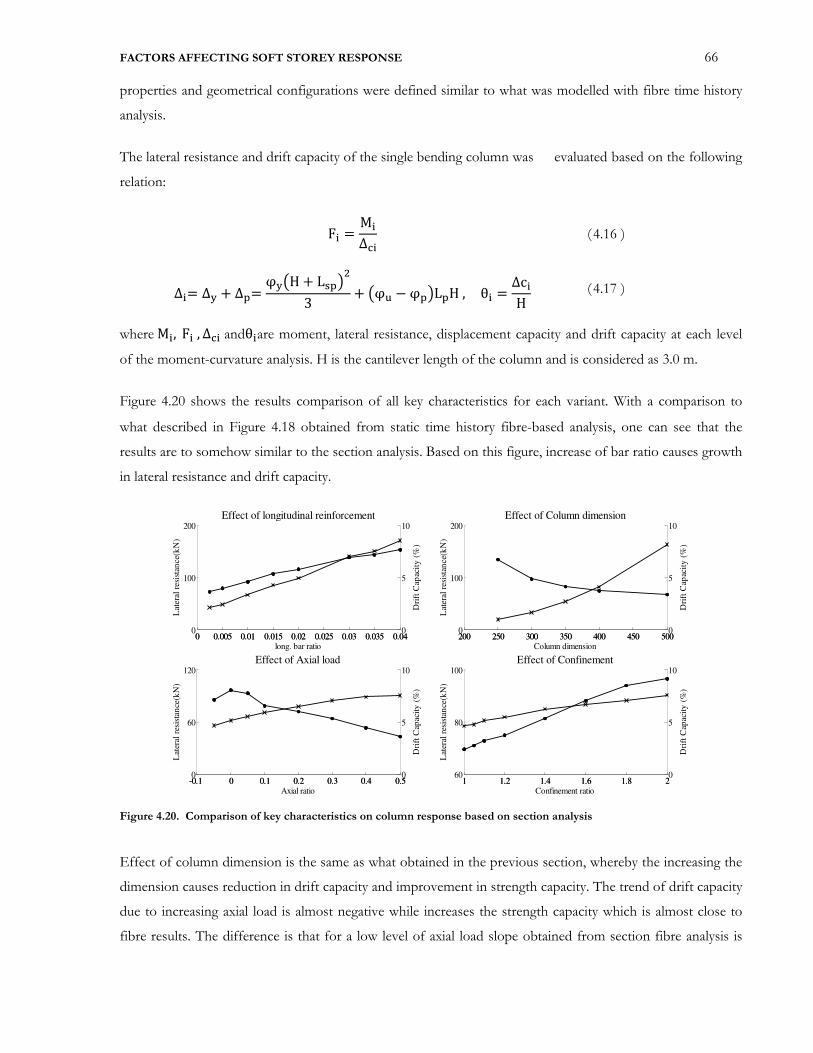
FACTORS AFFECTING SOFT STOREY RESPONSE 66
properties and geometrical configurations were defined similar to what was modelled with fibre time history
analysis.
The lateral resistance and drift capacity of the single bending column was evaluated based on the following
relation:
Fx = Mx∆/x ( 4.16 )
∆x= ∆¨ + ∆3= φ¨¹H + L>3¼�3 + ¹φ= − φ3¼L3H , θx = ∆cxH ( 4.17 )
where Mx, Fx , ∆/x andθxare moment, lateral resistance, displacement capacity and drift capacity at each level
of the moment-curvature analysis. H is the cantilever length of the column and is considered as 3.0 m.
Figure 4.20 shows the results comparison of all key characteristics for each variant. With a comparison to
what described in Figure 4.18 obtained from static time history fibre-based analysis, one can see that the
results are to somehow similar to the section analysis. Based on this figure, increase of bar ratio causes growth
in lateral resistance and drift capacity.
Figure 4.20. Comparison of key characteristics on column response based on section analysis
Effect of column dimension is the same as what obtained in the previous section, whereby the increasing the
dimension causes reduction in drift capacity and improvement in strength capacity. The trend of drift capacity
due to increasing axial load is almost negative while increases the strength capacity which is almost close to
fibre results. The difference is that for a low level of axial load slope obtained from section fibre analysis is
0 0.005 0.01 0.015 0.02 0.025 0.03 0.035 0.040
100
200
long. bar ratio
Effect of longitudinal reinforcement
Lat
eral
res
ista
nce
(kN
)
0 0.005 0.01 0.015 0.02 0.025 0.03 0.035 0.040
5
10
Dri
ft C
apac
ity
(%
)
200 250 300 350 400 450 5000
100
200
Column dimension
Effect of Column dimension
Lat
eral
res
ista
nce
(kN
)
200 250 300 350 400 450 5000
5
10
Dri
ft C
apac
ity
(%
)
-0.1 0 0.1 0.2 0.3 0.4 0.50
60
120
Axial ratio
Effect of Axial load
Lat
eral
res
ista
nce
(kN
)
-0.1 0 0.1 0.2 0.3 0.4 0.50
5
10
Dri
ft C
apac
ity
(%
)
1 1.2 1.4 1.6 1.8 260
80
100
Confinement ratio
Effect of Confinement
Lat
eral
res
ista
nce
(kN
)
1 1.2 1.4 1.6 1.8 20
5
10
Dri
ft C
apac
ity
(%
)
FACTORS AFFECTING SOFT STOREY RESPONSE 67
positive, while in section analysis is almost flat. Effect of confinement ratio is also close for both analyses,
where increasing confinement improves drift capacity without significant effect on lateral resistance.
4.5.6 Effect of column characteristics on the demand to capacity ratio
In this section, the displacement demand-capacity ratio DDCR of reinforcement concrete columns is
obtained, and the effect of each key characteristic is investigated on this ratio.
The effective stiffness of the cantilever column, ½¾¾ , is the lateral resistance divided by displacement
capacity. Thus, the effective period ¿½¾¾will be calculated as Equation 4.17 :
½¾¾ = Y³!´�³À �´EjE!³{·´�jEÁÀ³·´�´{! �³Á³·j!� = O∆* , ¿½¾¾ = 2Â� MKÃÄÄ ( 4.18 )
where M is the mass of the single degree freedom of the column.
The demand displacement of the system for the determined effective period, ∆� , is obtained from the
inelastic displacement spectra. The spectral displacement reduction factor is determined from the following
relationship:
Å� = � 0.070.02 + Æ½Ç ( 4.19 )
where ƽÇis the equivalent damping estimated by the following relation [Priestley et al. 2007]:
Æ½Ç = 0.05 + 0.444 o − 1o ( 4.20 )
where o is the system ductility obtained from the ratio of displacement capacity by the yield displacement ∆£.
The value of 0.444 is adopted because the Takeda thin model coule better represent columns under high axial
loads. The yield displacement for a cantilever column with a single fixed condition is calculated as:
μ = ∆*'£^* , '¨ = ∅£Y3 ( 4.21 )
where ∅£ is the yield curvature of the column section. For a rectangular RC column section is estimated by
the following relation. ^* is the column cantilever height.
∅£ = 2.1 ¢£� ( 4.22 )
Demand displacement can be now determined from the reduced spectral displacement as: Δ� = Å�Ê�.
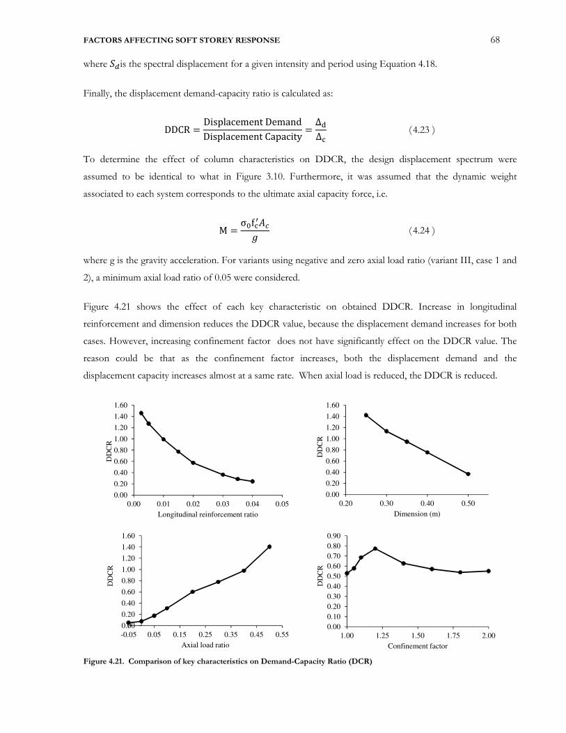
FACTORS AFFECTING SOFT STOREY RESPONSE 68
where �is the spectral displacement for a given intensity and period using Equation 4.18.
Finally, the displacement demand-capacity ratio is calculated as:
DDCR = Displacement DemandDisplacement Capacity = ΔÎΔ/ ( 4.23 )
To determine the effect of column characteristics on DDCR, the design displacement spectrum were
assumed to be identical to what in Figure 3.10. Furthermore, it was assumed that the dynamic weight
associated to each system corresponds to the ultimate axial capacity force, i.e.
M = σ�f/?X*Ï ( 4.24 )
where g is the gravity acceleration. For variants using negative and zero axial load ratio (variant III, case 1 and
2), a minimum axial load ratio of 0.05 were considered.
Figure 4.21 shows the effect of each key characteristic on obtained DDCR. Increase in longitudinal
reinforcement and dimension reduces the DDCR value, because the displacement demand increases for both
cases. However, increasing confinement factor does not have significantly effect on the DDCR value. The
reason could be that as the confinement factor increases, both the displacement demand and the
displacement capacity increases almost at a same rate. When axial load is reduced, the DDCR is reduced.
Figure 4.21. Comparison of key characteristics on Demand-Capacity Ratio (DCR)
0.00
0.20
0.40
0.60
0.80
1.00
1.20
1.40
1.60
0.00 0.01 0.02 0.03 0.04 0.05
DD
CR
Longitudinal reinforcement ratio
0.00
0.20
0.40
0.60
0.80
1.00
1.20
1.40
1.60
-0.05 0.05 0.15 0.25 0.35 0.45 0.55
DD
CR
Axial load ratio
0.00
0.20
0.40
0.60
0.80
1.00
1.20
1.40
1.60
0.20 0.30 0.40 0.50
DD
CR
Dimension (m)
0.00
0.10
0.20
0.30
0.40
0.50
0.60
0.70
0.80
0.90
1.00 1.25 1.50 1.75 2.00
DD
CR
Confinement factor
FACTORS AFFECTING SOFT STOREY RESPONSE 69
4.6 DISCUSSION OF RESULTS
This work began by comparing the behaviour of two RC frame buildings in Chapter 3 (variant 1 and variant 2
of Figure 3.1) that differed only by the fact that one had masonry infill from the first floor upwards whereas
the other had masonry infill over its full height. Results of incremental dynamic analyses tend to indicate that
the full masonry infill case could sustain much larger ground motion intensities when considering the collapse
limit state. This might encourage structural engineers faced with the task of retrofitting the partial infill
building to consider adding infills to the ground storey to render the structure similar to variant 1.
While this option may help in reducing the probability of collapse, it would not necessarily reduce the damage
and losses expected in the building for low to moderate earthquake intensities. This is partly because the floor
accelerations for the infill case are likely to be higher than in the partial infill case but in addition, it is well
known that damage to infill masonry occurs at much lower levels of drift than traditional RC frame
structures, with masonry infills requiring repair at drifts as low as 0.3% [Hak et al. 2012]. In addition, the open
ground storey scenario would have a lower probability of reaching a partial-collapse limit state associated with
masonry failure out-of-plane.
In addition to the points made above, it is recognised that the decision to retrofit a structure or not should be
made within a risk assessment framework in which the probability of different levels of seismic intensity is
considered along with the probable losses for each intensity level. With this in mind, it was decided that the
effect of different structural characteristics on the seismic vulnerability of RC frame structures with soft
storey mechanisms should be examined in more detail. As such, sections 4.2, 4.3 and 4.4 have, respectively,
examined the influence of P-delta effects, post yield stiffness ratio and the ground motion duration on the
drift and acceleration demands of the open-ground-storey structure, whereas Section 5 examined how
column dimensions, reinforcement contents and axial loads could affect deformation capacity.
The results of Section 4.2 have shown that P-delta effects will tend to increase the probability of collapse
significantly, increasing peak and residual drifts significantly, particularly at high intensities. This intuitive
observation is not yet well recognised by code assessment methods and therefore improvements to code
assessment procedures should be an area for future research. Furthermore, it suggests that soft-storey
structures could benefit from de-coupling of the gravity system from the lateral load resisting system. This
point will be discussed further in later paragraphs.
The results of Section 4.3 have instead shown that while an increased value of post-yield stiffness ratio does
help reduce both peak and residual drifts, the overall impact does not appear to be large. As such, while the
provision of some post-yield stiffness is important, it should not necessarily be a critical factor in retrofit
efforts for soft-storey structures.
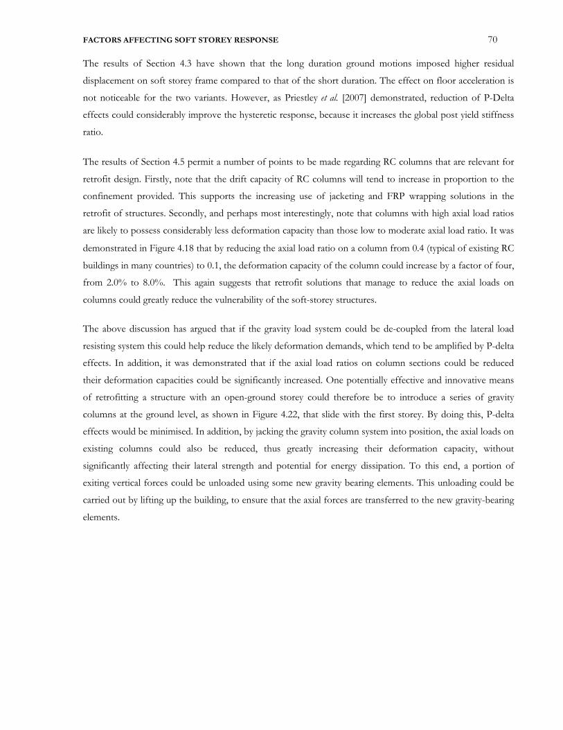
FACTORS AFFECTING SOFT STOREY RESPONSE 70
The results of Section 4.3 have shown that the long duration ground motions imposed higher residual
displacement on soft storey frame compared to that of the short duration. The effect on floor acceleration is
not noticeable for the two variants. However, as Priestley et al. [2007] demonstrated, reduction of P-Delta
effects could considerably improve the hysteretic response, because it increases the global post yield stiffness
ratio.
The results of Section 4.5 permit a number of points to be made regarding RC columns that are relevant for
retrofit design. Firstly, note that the drift capacity of RC columns will tend to increase in proportion to the
confinement provided. This supports the increasing use of jacketing and FRP wrapping solutions in the
retrofit of structures. Secondly, and perhaps most interestingly, note that columns with high axial load ratios
are likely to possess considerably less deformation capacity than those low to moderate axial load ratio. It was
demonstrated in Figure 4.18 that by reducing the axial load ratio on a column from 0.4 (typical of existing RC
buildings in many countries) to 0.1, the deformation capacity of the column could increase by a factor of four,
from 2.0% to 8.0%. This again suggests that retrofit solutions that manage to reduce the axial loads on
columns could greatly reduce the vulnerability of the soft-storey structures.
The above discussion has argued that if the gravity load system could be de-coupled from the lateral load
resisting system this could help reduce the likely deformation demands, which tend to be amplified by P-delta
effects. In addition, it was demonstrated that if the axial load ratios on column sections could be reduced
their deformation capacities could be significantly increased. One potentially effective and innovative means
of retrofitting a structure with an open-ground storey could therefore be to introduce a series of gravity
columns at the ground level, as shown in Figure 4.22, that slide with the first storey. By doing this, P-delta
effects would be minimised. In addition, by jacking the gravity column system into position, the axial loads on
existing columns could also be reduced, thus greatly increasing their deformation capacity, without
significantly affecting their lateral strength and potential for energy dissipation. To this end, a portion of
exiting vertical forces could be unloaded using some new gravity bearing elements. This unloading could be
carried out by lifting up the building, to ensure that the axial forces are transferred to the new gravity-bearing
elements.
FACTORS AFFECTING SOFT STOREY RESPONSE 71
Figure 4.22. Possible means of de-coupling gravidity loads from lateral loads in a soft storey building
4.7 SUMMARY AND CONCLUSION
The effect of some key characteristics on the behaviour of soft first storey buildings was explored. The case
studies assessed in the previous chapter were taken as the benchmark building and incremental non-linear
time history analyses were repeated varying some key parameters.
The analysis results indicated that P-Delta effects can considerably affect the vulnerability of partial infill RC
frames, although the effect depends on the intensity level. The influence of P-Delta effects is increased as the
intensity level is increased. Moreover, it was shown that high gravity loads related to P-Delta effects could be
very significant for moderate and high intensity levels, and greatly increases the potential collapse of soft
storey buildings. Although increasing the post-yield stiffness ratio of the first floor columns could be helpful
to reduce both peak and residual deformations at this level, it increases the seismic demand at storeys above
New gravity columns introduced to
slide with the overlying the structure
Connectionelement
FACTORS AFFECTING SOFT STOREY RESPONSE 72
this floor. This option might increase the retrofit cost of soft storey buildings. It was also demonstrated that,
at high intensity levels, long duration ground motions could increase the residual drift at the first floor of soft
storey buildings significantly.
The results of static cyclic analyses of RC columns with different geometrical and mechanical properties were
used to highlight the influence of some characteristics such as bar ratio, section dimensions, axial load ratio
and confinement factor on the lateral resistance and drift capacity of RC columns. The trends observed are
considered to be helpful in assessing the potential vulnerability of RC frame structures in which soft-storeys
are expected to develop at the ground floor.
The implications of the analysis findings were discussed in relation to potential retrofit schemes. A novel
retrofit scheme was proposed in which sliding gravity columns were introduced to reduce the impact of P-
Delta effects on displacement demands and to increase the deformation capacity of existing columns. That
the detailed design and development of this type proposed system is not presented hers as it is out of the
scope of this thesis. The next chapter will briefly discuss the limitation of this proposed retrofitting strategy.
As such, an alternative solution (gapped inclined brace GIB system) is proposed that reduces the drawbacks
of this proposal, while takes the positive aspects.

73
5.GAPPED INCLINED BRACE SYSTEM TO RETROFIT SOFT STOREY
BUILDINGS
5.1 INTRODUCTION
The results of the Chapter 4 suggested a potential retrofit strategy for open ground storey buildings in which
a portion of the existing vertical forces carried by the columns is transferred to new added gravity bearing
elements that slide with the first storey. This solution (Figure 5.1.a), however requires significant effort and
cost to lift the structure to ensure that the axial forces are transferred to the new gravity-bearing elements.
Moreover, because the lifting may not applied to all gravity elements simultaneously, it may also cause
unsymmetrical settlement to the existing columns, and foundation during the building lifetime. In addition,
the residual drift might not be reduced significantly when using such a retrofit strategy.
The results of the Chapter 4 suggested a potential retrofit strategy for open ground storey buildings in which
a portion of the existing vertical forces carried by the columns is transferred to new added gravity bearing
elements that slide with the first storey. This solution (Figure 5.1.a), however requires significant effort and
cost to lift the structure to ensure that the axial forces are transferred to the new gravity-bearing elements.
Moreover, because the lifting is not applied to all gravity elements simultaneously, it may also cause
unsymmetrical settlement to the existing columns, and foundation during the building lifetime. In addition,
the residual drift might not be reduced significantly when using such a retrofit strategy.
Alternatively, this chapter proposes the gapped-inclined brace (GIB), which consists of an elastic inclined
brace with a carefully selected gap element (Figure 5.1.b), to enhance the displacement capacity of the soft
floor while not increasing its lateral resistance. This is achieved by a mechanism that props and lifts the
structure during the earthquake, in effect using the input seismic energy to achieve an axial unloading of the
existing columns as the structure sways laterally. The GIB is installed at the ground level without inducing any
force on the existing elements. During the lateral motion of the building, the lateral movement of the
existing columns induces an axial shortening of the GIB, as illustrated in Figure 5.1.b. The gap inside the GIB
closes once the first floor displacement exceeds a critical value. This critical displacement is set by considering
either P-Delta effects or column deformation limits at the first floor. As the retrofit strategy is designed to
avoid adding significant lateral resistance to the structure, the building remains subject to low accelerations on
the floors above the soft storey when the lateral movement is controlled.

GAPPED INCLINED BRACE SYSTEM TO RETROFIT SOFT STOREY BUILDINGS 74
(a) (b)
Figure 5.1. Proposed mitigation strategies, a) roller system b) gapped inclined braced (GIB) system
Once the gap is closed, the GIB activates, and begins to share the vertical and the lateral load with the
existing columns. As the lateral displacement increases, the axial load on the first storey columns is carefully
reduced by the GIB so that, first, it counteracts the P-Delta effect, and second, it increases the lateral
deformation capacity of the first storey columns. At each level of lateral displacement, the axial load on the
columns that meets these two requirements is referred to as the effective axial force effP .
The advantage of this approach with respect to traditional brace retrofit solutions is that the retrofit strategy
does not shift the weakest point in the structure elsewhere (which would necessitate retrofitting measures in
the new location of the “weakest-link”) and is not very intrusive. Its advantage in comparison to installing
rollers, as suggested in Chapter 4, is that there is no need to uplift the building, which obviously represents
significant time and cost advantages.
To develop this retrofit scheme, in Section 5.1, the effective axial load effP to counteract P-Delta effects is
first derived. In Section 5.2, the effP for RC columns is obtained, and consequently, the details of the
proposed system are then defined such that it achieves the desired effP in Section 5.4. Section 5.5 describes the
mechanics of the hybrid system (RC column and Gapped-Inclined Brace, GIB) and derives the equations that
govern the response. In Section 5.6 a systematic design procedure are then explained and illustrated, and the
theoretical relations that are derived are verified through nonlinear pushover analyses. In Section 5.7 a
Initial condition Initial condition
Ultimate condition Initial condition
Residual condition Residual condition
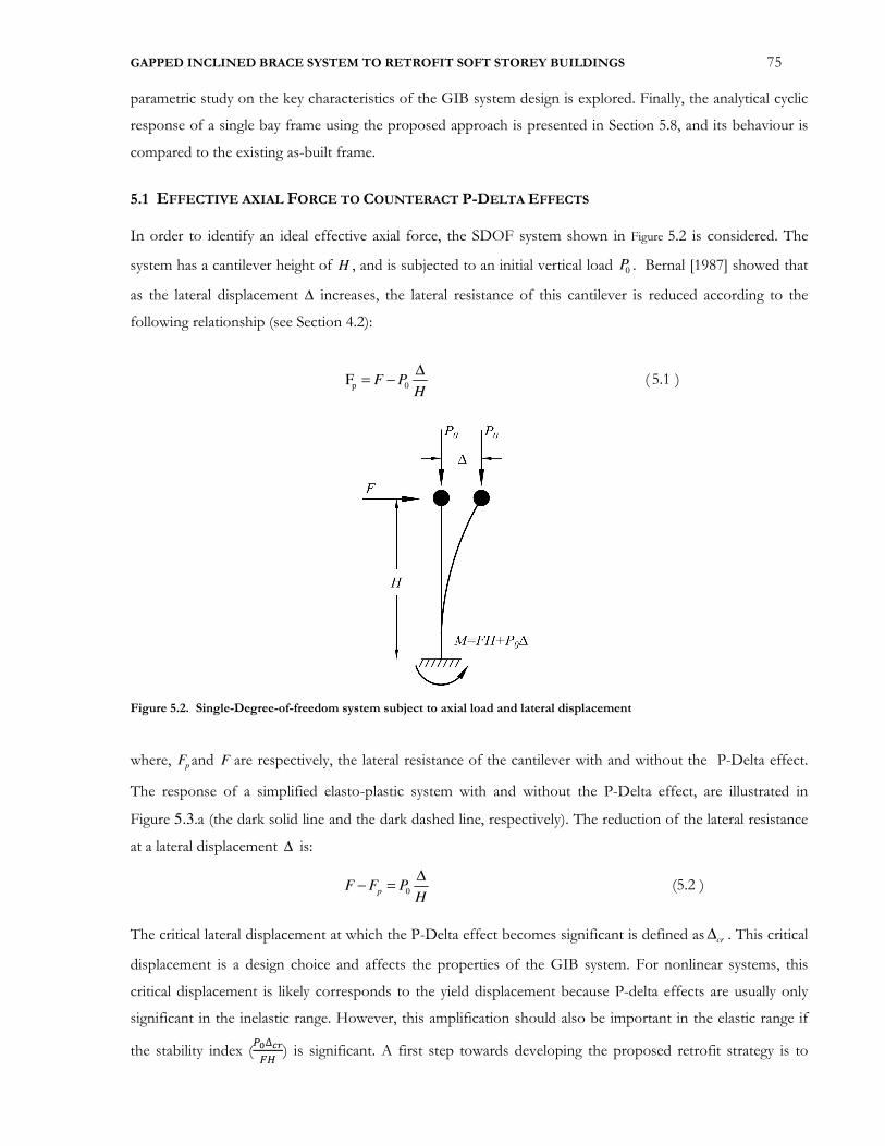
GAPPED INCLINED BRACE SYSTEM TO RETROFIT SOFT STOREY BUILDINGS 75
parametric study on the key characteristics of the GIB system design is explored. Finally, the analytical cyclic
response of a single bay frame using the proposed approach is presented in Section 5.8, and its behaviour is
compared to the existing as-built frame.
5.1 EFFECTIVE AXIAL FORCE TO COUNTERACT P-DELTA EFFECTS
In order to identify an ideal effective axial force, the SDOF system shown in Figure 5.2 is considered. The
system has a cantilever height of H , and is subjected to an initial vertical load 0P . Bernal [1987] showed that
as the lateral displacement ∆ increases, the lateral resistance of this cantilever is reduced according to the
following relationship (see Section 4.2):
p 0F F PH
∆= − ( 5.1 )
Figure 5.2. Single-Degree-of-freedom system subject to axial load and lateral displacement
where, pF and F are respectively, the lateral resistance of the cantilever with and without the P-Delta effect.
The response of a simplified elasto-plastic system with and without the P-Delta effect, are illustrated in
Figure 5.3.a (the dark solid line and the dark dashed line, respectively). The reduction of the lateral resistance
at a lateral displacement ∆ is:
0pF F P
H
∆− = ( 5.2 )
The critical lateral displacement at which the P-Delta effect becomes significant is defined as cr∆ . This critical
displacement is a design choice and affects the properties of the GIB system. For nonlinear systems, this
critical displacement is likely corresponds to the yield displacement because P-delta effects are usually only
significant in the inelastic range. However, this amplification should also be important in the elastic range if
the stability index (�Ð∆ÑÒÓÔ ) is significant. A first step towards developing the proposed retrofit strategy is to

GAPPED INCLINED BRACE SYSTEM TO RETROFIT SOFT STOREY BUILDINGS
define effP such that it counteracts the P
reduction of the second roder lateral resistance (
This results in:
eff 0P ,
Since P-Delta effects are assumed to be insignificant
Assuming that cr y∆ = ∆ , to identify the desired
inelastic range, the axial load effP
point (Figure 5.3.b); then, the axial load should be reduced following
that when the P-Delta effect is counteracted in this manner, the initial lateral response of the system dra
with the dark dashed line in Figure
same figure.
Figure 5.3 a) Influence of the P-Delta effect and the
GAPPED INCLINED BRACE SYSTEM TO RETROFIT SOFT STOREY BUILDINGS
such that it counteracts the P-Delta effect for displacements greater than cr∆
lateral resistance ( effPH
∆) is maintained at a value as close as possible
eff 0P ,cr
crP
H H
∆∆= ∆ > ∆ ( 5.
assumed to be insignificant for displacements smaller than cr∆
eff 0
eff 0
P ,
P ,
cr
cr
cr
P
P
= ∆ ≤ ∆ ∆
= ∆ > ∆ ∆
( 5.
, to identify the desired effP that would counteract the P-Delta effect within the
eff should be equal to the initial axial load 0P until the system reaches the yield
.b); then, the axial load should be reduced following eff 0P ,y
P∆
= ∆ > ∆∆
Delta effect is counteracted in this manner, the initial lateral response of the system dra
Figure 5.3.a is altered to a response that is illustrated by the light solid line in the
Delta effect and the effP on the force-displacement response b) Effective axial force (
76
cr∆ . This requires that the
) is maintained at a value as close as possible to 0
crPH
∆.
.3 )
cr∆ , effP is given by
.4 )
Delta effect within the
until the system reaches the yield
y= ∆ > ∆ . Figure 5.3.a shows
Delta effect is counteracted in this manner, the initial lateral response of the system drawn
illustrated by the light solid line in the
displacement response b) Effective axial force ( effP )

GAPPED INCLINED BRACE SYSTEM TO RETROFIT SOFT STOREY BUILDINGS 77
5.2 EFFECT OF AXIAL LOADS ON THE DEFORMATION CAPACITY OF RC COLUMNS
Irrespectively of P-Delta effects, axial loads can have a negative effect on the deformation capacity of RC
columns [Paulay and Priestley 1992; Fardis and Biskinis 2003; Lam et al. 2003]. As such, the ideal effective
axial load should also consider column sectional resistance.
To achieve the desired effP , the response of a typical 0.40 0.40× m RC column with 3.0 m cantilever height,
longitudinal reinforcement ratio of 0.01 and confinement factor of 1.15 is determined through moment
curvature analyses for various axial load ratios ( '
0 gσ P /A f c= σ = ÕÖ×Ä′/) ranging from 0.01 to 0.5 in increments
of 0.02. The compressive strength of the concrete 'f c and the rebar yield strength fys are assumed 20 MPa,
and 370 MPa, respectively. The Mander model [Mander et al. 1988] is used to evaluate constitutive relations
for the confined and the unconfined concrete in compression. For what concerns the constitutive relations
for reinforcement steel, the model proposed by King et al. [1986] is adopted. The strain at maximum stress
for unconfined concrete is assumed 0.002, while the ultimate concrete strain is governed by the core crushing
limit state proposed by Kowalsky [2000], and the ultimate tensile strain of the reinforcement is assumed as
12%. The lateral displacement of the cantilever was estimated using the simplified lumped plasticity approach
using Equation 5.5 as the sum of the elastic and plastic deformations.
2( )( )
3
y sp
u y p
H LL H
ϕϕ ϕ
+∆ = + − ( 5.5 )
where yϕ and uϕ are the yield and ultimate curvature, respectively; H is the cantilever height of the RC
columns; spL and p
L are strength penetration length and the plastic hinge length, and were estimated from
equations proposed by Priestley et al. [2007]. The lateral resistance of the RC column was calculated by
dividing the moment resistance obtained from the section analyses by the cantilever height.
The dotted line in Figure 5.4.a indicates the variation in the maximum lateral drift capacity ratio versus the
axial load ratio. The lateral drift capacity decreases almost linearly when the axial load ratio increases. An
increase in the axial load ratio from 0.1 to 0.5 leads to a reduction in the drift capacity from 9.0% to almost
4.0%. However, P-Delta effects were not considered in calculating the relationship between the axial load and
the drift capacity ratio of the RC column.
5.3 effP FOR RC COLUMNS
To consider the influence of P-Delta effects, the lateral resistance was reduced based on Equation 5.1. The
analysis stopped when the lateral resistance reduced to 70% of the yield resistance. This value corresponds to
a stability coefficient of 0.3, which is recommended by many current seismic codes [FEMA 1997; ATC
2007a] as an upper bound limit.
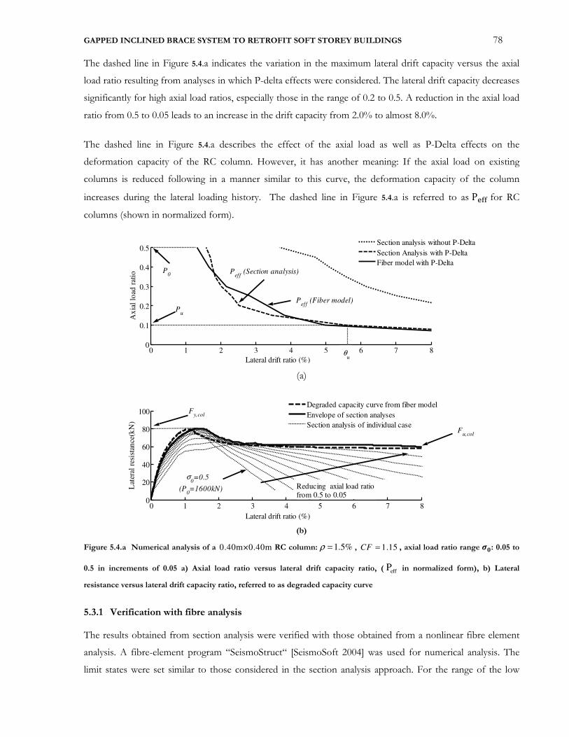
GAPPED INCLINED BRACE SYSTEM TO RETROFIT SOFT STOREY BUILDINGS 78
The dashed line in Figure 5.4.a indicates the variation in the maximum lateral drift capacity versus the axial
load ratio resulting from analyses in which P-delta effects were considered. The lateral drift capacity decreases
significantly for high axial load ratios, especially those in the range of 0.2 to 0.5. A reduction in the axial load
ratio from 0.5 to 0.05 leads to an increase in the drift capacity from 2.0% to almost 8.0%.
The dashed line in Figure 5.4.a describes the effect of the axial load as well as P-Delta effects on the
deformation capacity of the RC column. However, it has another meaning: If the axial load on existing
columns is reduced following in a manner similar to this curve, the deformation capacity of the column
increases during the lateral loading history. The dashed line in Figure 5.4.a is referred to as PÃÄÄ for RC
columns (shown in normalized form).
(a)
(b)
Figure 5.4.a Numerical analysis of a 0.40m×0.40m RC column: 1.5%ρ = , 1.15CF = , axial load ratio range ÙP: 0.05 to 0.5 in increments of 0.05 a) Axial load ratio versus lateral drift capacity ratio, ( effP in normalized form), b) Lateral
resistance versus lateral drift capacity ratio, referred to as degraded capacity curve
5.3.1 Verification with fibre analysis
The results obtained from section analysis were verified with those obtained from a nonlinear fibre element
analysis. A fibre-element program “SeismoStruct“ [SeismoSoft 2004] was used for numerical analysis. The
limit states were set similar to those considered in the section analysis approach. For the range of the low
0 1 2 3 4 5 6 7 80
0.1
0.2
0.3
0.4
0.5
Ax
ial
load
rat
io
Section analysis without P-Delta
Section Analysis with P-Delta
Fiber model with P-Delta
Pu
P0
θuLateral drift ratio (%)
Peff
(Fiber model)
Peff
(Section analysis)
0 1 2 3 4 5 6 7 80
20
40
60
80
100
Lat
eral
res
ista
nce
(kN
)
Degraded capacity curve from fiber model
Envelope of section analyses
Section analysis of individual case
Fy,col
(P0=1600kN)
σ0=0.5
Lateral drift ratio (%)
Fu,col
Reducing axial load ratio from 0.5 to 0.05
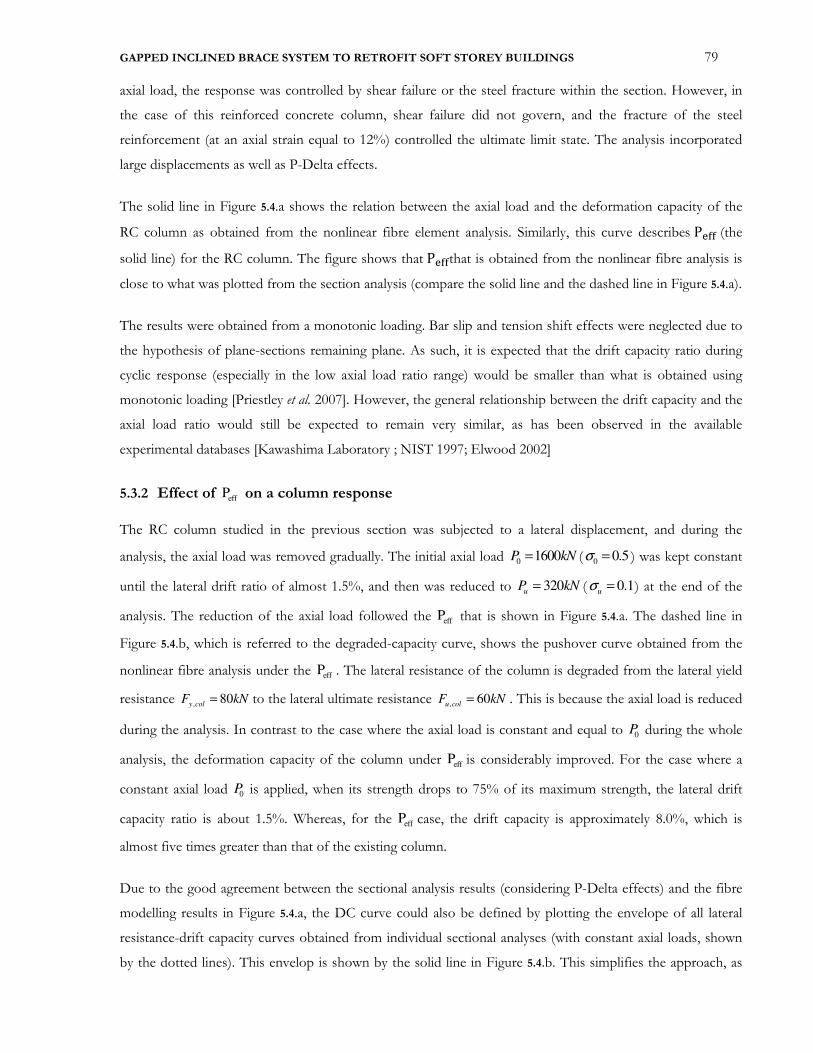
GAPPED INCLINED BRACE SYSTEM TO RETROFIT SOFT STOREY BUILDINGS 79
axial load, the response was controlled by shear failure or the steel fracture within the section. However, in
the case of this reinforced concrete column, shear failure did not govern, and the fracture of the steel
reinforcement (at an axial strain equal to 12%) controlled the ultimate limit state. The analysis incorporated
large displacements as well as P-Delta effects.
The solid line in Figure 5.4.a shows the relation between the axial load and the deformation capacity of the
RC column as obtained from the nonlinear fibre element analysis. Similarly, this curve describes PÃÄÄ (the
solid line) for the RC column. The figure shows that PÃÄÄthat is obtained from the nonlinear fibre analysis is
close to what was plotted from the section analysis (compare the solid line and the dashed line in Figure 5.4.a).
The results were obtained from a monotonic loading. Bar slip and tension shift effects were neglected due to
the hypothesis of plane-sections remaining plane. As such, it is expected that the drift capacity ratio during
cyclic response (especially in the low axial load ratio range) would be smaller than what is obtained using
monotonic loading [Priestley et al. 2007]. However, the general relationship between the drift capacity and the
axial load ratio would still be expected to remain very similar, as has been observed in the available
experimental databases [Kawashima Laboratory ; NIST 1997; Elwood 2002]
5.3.2 Effect of effP on a column response
The RC column studied in the previous section was subjected to a lateral displacement, and during the
analysis, the axial load was removed gradually. The initial axial load 0 1600P kN= ( 0 0.5σ = ) was kept constant
until the lateral drift ratio of almost 1.5%, and then was reduced to 320uP kN= ( 0.1uσ = ) at the end of the
analysis. The reduction of the axial load followed the effP that is shown in Figure 5.4.a. The dashed line in
Figure 5.4.b, which is referred to the degraded-capacity curve, shows the pushover curve obtained from the
nonlinear fibre analysis under the effP . The lateral resistance of the column is degraded from the lateral yield
resistance , 80y col
NF k= to the lateral ultimate resistance , 60colu
NF k= . This is because the axial load is reduced
during the analysis. In contrast to the case where the axial load is constant and equal to 0P during the whole
analysis, the deformation capacity of the column under effP is considerably improved. For the case where a
constant axial load 0P is applied, when its strength drops to 75% of its maximum strength, the lateral drift
capacity ratio is about 1.5%. Whereas, for the effP case, the drift capacity is approximately 8.0%, which is
almost five times greater than that of the existing column.
Due to the good agreement between the sectional analysis results (considering P-Delta effects) and the fibre
modelling results in Figure 5.4.a, the DC curve could also be defined by plotting the envelope of all lateral
resistance-drift capacity curves obtained from individual sectional analyses (with constant axial loads, shown
by the dotted lines). This envelop is shown by the solid line in Figure 5.4.b. This simplifies the approach, as
GAPPED INCLINED BRACE SYSTEM TO RETROFIT SOFT STOREY BUILDINGS 80
there is no requirement to run several pushover analyses with fibre modelling. The degraded-capacity curves
obtained from both approaches are close to each other. However, results are slightly different in the high
axial load range (low deformation capacity). The lateral resistance from the section analysis starts to reduce at
a drift ratio of 1.2%, while this value is 1.0% based on fibre modelling. The difference could be due to
assumptions considered in each approach, which is a source of uncertainty. However, the overall match can
be considered acceptable as they have similar behaviour in the lower axial load ranges, which are being
targeted because of the higher deformation capacity they given the columns.
5.4 PROPOSAL OF A GAPPED INCLINED BRACE TO ACHIEVE THE effP
To achieve the desired effP within a retrofit strategy, a Gapped-Inclined Brace (GIB), composed of an inclined
brace fitted with a carefully selected gap, could be installed at the ground level without inducing any force to
the exiting elements, as shown in Figure 5.5.a The lateral movement of the existing column results in an
elastic rotation of the GIB system. The gap is required to limit the increase of the lateral strength of the
system caused by the GIB. When the gap is closed, the GIB activates, and shares the vertical and lateral load
with the existing column. The lateral resistance provided by the GIB compensates for the lateral strength
degradation of the columns that occurs due to the reduction of their axial load.
(a) (b) (c)
Figure 5.5. Gapped-Inclined Brace (GIB) system to the existing column a) Initial condition b) Closing gap condition c)
Ultimate condition
Figure 5.5.c illustrates the deformed state of the hybrid system when the ultimate displacement is reached.
However, it is conservative if the ultimate displacement demand of the whole system is reached before the
GIB reaches the vertical position. Mechanics of the GIB system
Lb
Gap Gap is closedGap isopenned
P P P
Lb0
Inclined
brace

GAPPED INCLINED BRACE SYSTEM TO RETROFIT SOFT STOREY BUILDINGS 81
5.5 MECHANICS OF THE GIB SYSTEM
As the next step within the retrofit strategy of soft storey buildings, the GIB should be carefully designed so
that the desired effP is achieved as the floor sways laterally. The properties of the GIB are defined based on
three major parameters: The initial angle of the GIB , GIBθ , the gap distance GIB∆ , and the mechanical
properties of the inclined brace. These parameters are obtained based on a free-end column condition to
simplify the problem and to illustrate the purposes of the proposed strategy. However, the equations that are
derived can be directly extended to fixed-end column conditions, which is a better representation of columns
at the ground level. In this derivation, the column is assumed to behave as a cantilever before the gap is
closed (Figure 5.6.a), and its lateral deformation can be easily calculated. As a simplification, it is assumed that
once the gap is closed, the plastic hinge is formed at the end of the column, while the rest of the column
rotates without any plastic flexural deformation, as shown in Figure 5.6.b and Figure 5.6.c.
Figure 5.6. Mechanics of the GIB system a) Initial position, b) elastic behaviour of the column before gap is closed c) post
yield condition
5.5.1 Initial position of the GIB
The distance between the existing column and GIB , GIB∆ (or more precisely, the brace angle) can control the
total lateral resistance of the system. The lateral resistance of the GIB should ideally compensate for the
∆GIB
Hc
∆cr − ∆y
∆u ∆r
∆v
∆vy− 0
LGIB=Lb0+∆gap
∆gap
Lb0
Lb
LcθGIB
θ y
(a) (b) (c)
∆GIB ∆GIB
~
B C
A
B CC B
A
A
θ u
θ r
~
Not to scale
F
P0
F F
θGIB-θ y θ r=θGIB-θ uθGIB
PGIB=(P0-Pucosθ u)/cosθ r
P0 P0
PG
IB =0
PG
IB =0 P
u
Pc=
P0
Pc=
P0
A A A

GAPPED INCLINED BRACE SYSTEM TO RETROFIT SOFT STOREY BUILDINGS 82
lateral strength degradation of the column, which decreases from the yield strength ,y
V col to the ultimate
strength ,uV col .
, ,GIB r y col u colP Fs n ) Fi (θ = − ( 5.6.a )
where rθ is the angle of the GIB with respect to the vertical axis at the ultimate state (Figure 5.6.c). The
vertical component of the GIB axial force GIB rcos( )P θ is the difference between the initial axial force of the
column 0 P and its vertical component at the ultimate states GIB r 0 u ucos( ) sP P - P coθ θ= (Figure 5.7):
GIB r 0 u ucos( ) sP P - P coθ θ= ( 5.6.b )
Figure 5.7. Effect of the GIB on the lateral resistance and the displacement capacity of RC columns
where uθ is the ultimate lateral drift capacity of the column. Dividing Equation 5.6.a by Equation 5.6.b and
assuming that 0 u u 0 ucosP - P P - Pθ ≈ , and r GIB uθ θ θ= − , the initial angle of the GIBθ , shown in Figure 5.6, is
given by
y,col u,col-1
GIB u
0 u
F - Ftan +
P - P,θ θ= ( 5.7 )
The distance between the base of the GIB and the column centreline GIB∆ (node B to node C in Figure 5.6) is
y,col u,col-1
GIB u
0 u
F - Ftan +
P - P,θ θ= ( 5.8 )
Lat
eral
res
ista
nce
Lateral drift ratio
GIB
Fu,col
Fy,col
θgc
Column
Lateral resistance of
the GIB: FGIB=PGIB sinθr
θcr (controlled by the gap)
θGIB
Lateral degradation of
the RC column: Fy,col - Fu,col
θu
GIB compansates for the
degradation: FGIB=Fy,col-Fu,col
θr=θGIB-θu
GAPPED INCLINED BRACE SYSTEM TO RETROFIT SOFT STOREY BUILDINGS 83
Figure 5.7 also demonstrates the effect of the GIB on the lateral resistance and the deformation capacity of
RC columns. The lateral force could also be controlled by varying the gap distance as it controls the effP in the
GIB, which is explained in the next paragraphs.
5.5.2 Gap distance
The role of the gap element is important as it controls the point at which the lateral resistance of the existing
column starts to decrease. If the gap distance is more than required, the delay in the unloading of the existing
column may cause the overloading of the column, and also increase the residual displacement. However, if
the gap is too small, the lateral resistance of the system starts to increase before than the lateral resistance of
the column starts to decrease. This increases the total lateral resistance of the first floor, which would
consequently increase the seismic demands that are transferred to the upper storeys. However, a small gap
distance could change the column mechanism from being mainly flexure/shear with some axial force, to
being mainly axial, which might be an effective solution in cases where columns are critical in shear but this
aspect is not examined here.
As a result of this retrofit strategy, the lateral drift ratio corresponding to a closed gap gcθ can be obtained
from the two following conditions:
a) gcθ controls the lateral resistance at the ultimate state. In this case uθ in Figure 5.7 should occur when the
lateral resistance of the GIB is maximized, i.e., ) / 2(r GIB gc
θ θ θ= − , Thus, since r GIB uθ θ θ= − , the lateral drift
ratio once the gap is closed gcθ is given by
2gc u GIB
θ θ θ= − ( 5.9 )
b) gcθ controls the critical lateral drift ratio of existing columns. In this case, gc cr
θ θ= . In many cases, this
condition governs, and could conservatively be considered as the yield drift ratio of the existing column yθ , at
which the lateral resistance starts to degrade (Figure 5.7).
The gap distance gap∆ is the difference between the initial length of the GIB, GIBL , and the length of the GIB
when the gap is closed 0bL ,i.e. 0gap GIB bL L∆ = − :
( ) ( )cos cos
c vyc
gap
GIB GIB gc
HH
θ θ θ∆ =
−
+−
∆ ( 5.10 )
where vy ∆ is the vertical displacement of the column at yield, which could be assumed negligible even though
this assumption is not likely to be very accurate for exterior columns.

GAPPED INCLINED BRACE SYSTEM TO RETROFIT SOFT STOREY BUILDINGS 84
5.5.3 Design of the inclined brace
From geometrical compatibility, the deformation of the inclined brace could be obtained from the difference
between its initial length and the length during the loading history
( )( )
( )( )0
cos
coscos
xc
b b b c C
GIB xGIB y
HL L L H L
θ
θ θθ θ∆ = − −= + ∆
−− ( 5.11 )
where c L∆ is the axial elongation of the existing column and could be considerable as the compressive force
of the column at the ultimate state is significantly reduced. Neglecting the concrete tension stiffness in the
plastic hinge region, the axial elongation of the column is obtained from the axial stiffness of the
reinforcement only in the plastic hinge area pK and the axial stiffness of the concrete in the rest of the
column elK .This assumption could only be appropriate for external columns, which are subjected to tension.
However, the accuracy could be reduced for middle columns and is a part of uncertainty. Considering this
assumption in mind, the axial elongation of RC columns in the GIB system could be estimated as:
0 , u
c c
c
P PL H
K
−∆ = ,
el p
C
el p
K KK
K K
×=
+, s s
p
p
E AK
L=
0.5
c C
el
c p
E AK
H L=
− ( 5.12 )
where uP is the axial force of the column obtained from the effP curve; iscK the axial stiffness of the
column. s cE and E are the modulus of elasticity of steel and concrete; st cA and A represent the reinforcement
area and the column cross section area, respectively. For low axial load ratio, the cracked area of the RC
column could lead to a better estimation. pL is the plastic hinge length, and could be estimated from
recommended equations [Priestley et al. 2007]. For typical columns with rebar ratio 0.01, s cE / E 10= and
plastic hinge length of 0.15 times the total column height (range is usually between 0.1 to 0.2), the column
axial deformation obtained from Equations 5.11 and 5.12 could be estimated as
0
. .
u
c c
c c
P PL H
E Aα
−∆ ≅ ( 5.13 )
where α is obtained as 0.4. For a fixed-end column, considering that the plastic hinges form at the two ends
of the column, α is estimated as 0.25. A parametric study is recommended as a part of the future research to
better estimate the effect of axial elongation of RC columns on the design parameters of the GIB system.
The axial force in the GIB is obtained from the equilibrium condition in the vertical axis
( )0
cos
u
b
GIB x
P PP
θ θ
−=
− ( 5.14 )
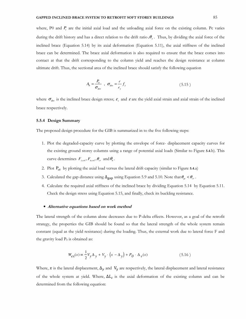
GAPPED INCLINED BRACE SYSTEM TO RETROFIT SOFT STOREY BUILDINGS 85
where, P0 and cP are the initial axial load and the unloading axial force on the existing column. Pc varies
during the drift history and has a direct relation to the drift ratio , xθ . Thus, by dividing the axial force of the
inclined brace (Equation 5.14) by its axial deformation (Equation 5.11), the axial stiffness of the inclined
brace can be determined. The brace axial deformation is also required to ensure that the brace comes into
contact at that the drift corresponding to the column yield and reaches the design resistance at column
ultimate drift. Thus, the sectional area of the inclined brace should satisfy the following equation
, b
b des y
des y
PA fσ
σ= =
ε
ε
( 5.15 )
where desσ is the inclined brace design stress; yε and ε are the yield axial strain and axial strain of the inclined
brace respectively.
5.5.4 Design Summary
The proposed design procedure for the GIB is summarized in to the five following steps:
1. Plot the degraded-capacity curve by plotting the envelope of force- displacement capacity curves for
the existing ground storey columns using a range of potential axial loads (Similar to Figure 5.4.b). This
curve determines ,,y,col u,col cr
F F θ and uθ .
2. Plot effP by plotting the axial load versus the lateral drift capacity (similar to Figure 5.4.a)
3. Calculated the gap distance using ∆rÚ3 using Equation 5.9 and 5.10. Note that gc crθ θ< .
4. Calculate the required axial stiffness of the inclined brace by dividing Equation 5.14 by Equation 5.11.
Check the design stress using Equation 5.15, and finally, check its buckling resistance.
• Alternative equations based on work method
The lateral strength of the column alone decreases due to P-delta effects. However, as a goal of the retrofit
strategy, the properties the GIB should be found so that the lateral strength of the whole system remain
constant (equal as the yield resistance) during the loading. Thus, the external work due to lateral force F and
the gravity load P0 is obtained as:
( 5.16 )
Where, ¯ is the lateral displacement, ∆£ and V¨ are respectively, the lateral displacement and lateral resistance
of the whole system at yield. Where, ∆Y* is the axial deformation of the existing column and can be
determined from the following equation:
Wex x( )1
2Vy ∆ y Vy x ∆ y−( )⋅+ P0 ∆ v x( )⋅+
GAPPED INCLINED BRACE SYSTEM TO RETROFIT SOFT STOREY BUILDINGS 86
The internal work is calculated due to the axial deformations of the column and the GIB in addition to the
flexural deformation of the existing column. Using lumped plasticity simplification, and assuming that the
column has an elastics-perfectly plastic behaviour, the internal work can be determined:
( 5.17 )
Where, '�, '£ and My are, respectively, the lateral rotation, and the yield rotation and the yield moment of the
existing column. ∆Y] is the axial deformation of the inclined brace, and �] is the axial force in the inclined
brace is estimated from equilibrium.
Thus, the axial deformation of the inclined brace can be obtained from the principle of the equal work
resulting from internal and external forces:
∆Y] = 0.5(�� + �)∆Y* − ��∆H − ��'£�(o − 0.5) *̂0.5�] ( 5.18 )
5.6 DESIGN EXAMPLE AND NUMERICAL VERIFICATION
The proposed design approach was applied to the RC concrete column that was studied previously; the
column was subjected to an initial axial load ratio of 0.5 such that the total axial load was 1600kN (column
dimension of 0.4 0.4× m, and a concrete compressive strength of 20MPa). As a first step towards defining the
properties of the GIB, the degraded-capacity curve of the column is determined according to the procedure
given earlier (Figure 5.4b). This curve indicated that the ultimate axial load is 320uP kN= ( 0.1)uσ = , which
corresponds to an ultimate lateral drift ratio of around 5.5%uθ = . At this drift ratio the lateral strength
degradation due to second order effects of the RC column is 15 kN (reduced from , 78y col
F kN= to
, 63u col
F kN= ). Thus, using Equation 5.7, the GIB should be located 201 mm from the centre of the column (
6.7%GIBθ = ).
The critical drift capacity crθ at which the lateral resistance starts to degrade is 1.2%, corresponding to a
stability coefficient of ,/ 1600 / 78 0.012 0.24P cr y col
P F Hθ ∆ = ∆ × = × = , which is less than the code limit of 0.3.
The drift ratio when the gap is closed is calculated as 4.3%cg
θ = , which is larger than crθ . Thus, using cg crθ θ=
,the gap distance and the axial deformation of the inclined brace is calculated as 2.7 mm and 5.8 mm using
Equations 5.10 and 5.11, respectively.
Win x( )1
2My θy⋅ My θ x( ) θy−( )⋅+
0.5Pb x( ) ∆L b x( )⋅+ 0.5 P0 P x( )+( ) ∆L c x( )⋅−
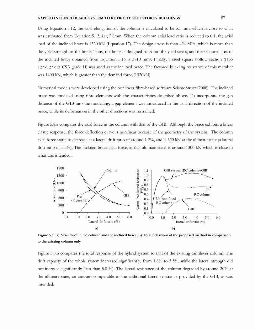
GAPPED INCLINED BRACE SYSTEM TO RETROFIT SOFT STOREY BUILDINGS 87
Using Equation 5.12, the axial elongation of the column is calculated to be 3.1 mm, which is close to what
was estimated from Equation 5.13, i.e., 2.8mm. When the column axial load ratio is reduced to 0.1, the axial
load of the inclined brace is 1320 kN (Equation 17). The design stress is then 424 MPa, which is more than
the yield strength of the brace. Thus, the brace is designed based on the yield stress, and the sectional area of
the inclined brace obtained from Equation 5.15 is 3710 mm2. Finally, a steel square hollow section (HSS
127 127 13× × CSA grade H) was used as the inclined brace. The factored buckling resistance of this member
was 1400 kN, which is greater than the demand force (1320kN).
Numerical models were developed using the nonlinear fibre-based software SeismoStruct (2008). The inclined
brace was modeled using fibre elements with the characteristics described above. To incorporate the gap
distance of the GIB into the modelling, a gap element was introduced in the axial direction of the inclined
brace, while its deformation in the other directions was restrained.
Figure 5.8.a compares the axial force in the column with that of the GIB. Although the brace exhibits a linear
elastic response, the force deflection curve is nonlinear because of the geometry of the system. The column
axial force starts to decrease at a lateral drift ratio of around 1.2%, and is 320 kN at the ultimate state (a lateral
drift ratio of 5.5%). The inclined brace axial force, at this ultimate state, is around 1300 kN which is close to
what was intended.
a) b)
Figure 5.8. a) Axial force in the column and the inclined brace, b) Total behaviour of the proposed method in comparison
to the existing column only
Figure 5.8.b compares the total response of the hybrid system to that of the existing cantilever column. The
drift capacity of the whole system increased significantly, from 1.6% to 5.5%, while the lateral strength did
not increase significantly (less than 5.0 %). The lateral resistance of the column degraded by around 20% at
the ultimate state, an amount comparable to the additional lateral resistance provided by the GIB, as was
intended.
0
300
600
900
1200
1500
1800
0.0 1.0 2.0 3.0 4.0 5.0 6.0
Ax
ial
forc
e (k
N)
Lateral drift ratio (%)
Column
GIBPeff
(Figure 4a)
0.0
0.1
0.3
0.4
0.5
0.6
0.8
0.9
1.0
1.1
0.0 1.0 2.0 3.0 4.0 5.0 6.0
No
rmal
ized
lat
eral
res
ista
nce
(F/F
y)
lateral drift ratio (%)
GIB
RC column
GIB system (RC column+GIB)
Un-retrofitted
RC column

GAPPED INCLINED BRACE SYSTEM TO RETROFIT SOFT STOREY BUILDINGS 88
5.7 PARAMETRIC STUDY
Figure 5.9 to Figure 5.11 illustrate the design parameters of the GIB system that are obtained following the same
procedure for various column configurations, considering different height, different initial axial load ratio and
different confinement conditions. Wherever one parameter is changed, other parameters are kept constant.
The reference values of the variables include a column dimension of 0.40 0.40m× , a longitudinal
reinforcement ratio of sρ = 0.015, an axial load ratio of 0σ =0.30, and a confinement factor of CF = 1.15.
Figure 5.9 indicate that as the column height increases, the both required gap∆ and GIB∆ increase, and
obviously, a stronger brace is required to avoid buckling.
Figure 5.9. Effect of the GIB system on response of 0.40x0.40m RC columns with different height H
It should be note that the initial axial load has the greatest effect on the inclined brace sizing; the brace
section thickness increases from 4.8 mm to 13 mm, due to the increase of axial load (Figure 5.10). The GIB∆ is
also increased, which requires larger gap distance. As the axial load increases the effect of the GIB system is
more obvious, which implies that the GIB system is more useful for columns with higher axial loads.
The confinement has a stronger influence on the gap distance as shown in Figure 5.11. When the confinement
increases, the drift at which the degradation takes place ( mθ ) increases due to the improvement of the column
post-yield stiffness. Moreover, the maximum drift capacity of the hybrid system increases. Thus, by
combination of the proposed GIB system and the confinement, the displacement capacity of the system can
be greatly improved. As will be discussed in the following section, the suggested detail connection of the GIB
system could improve the confinement condition at the top of the column.
0
20
40
60
80
100
0.0 1.0 2.0 3.0 4.0 5.0 6.0
Lat
eral
res
ista
nce
(k
N)
Drift ratio (%)
H=2.5 m, CF=1.15, σ0=0.3
0
20
40
60
80
0.0 1.0 2.0 3.0 4.0 5.0 6.0
Lat
eral
res
ista
nce
(k
N)
Drift ratio (%)
H=3.5 m, CF=1.15, σ0=0.3
∆GIB = 244 mm, ∆gap = 3.6mm
HSS 127 x 127 x 4.8
∆GIB = 215 mm, ∆gap = 2.8mm
HSS 127 x 127 x 4.8
0
15
30
45
60
0.0 1.0 2.0 3.0 4.0 5.0 6.0
Lat
eral
res
ista
nce
(k
N)
Drift ratio (%)
H=4.0 m F=1.15,σ0=0.3
∆GIB = 255 mm, ∆gap = 3.9mm
HSS 127 x 127 x 6.40
10
20
30
40
0.0 1.0 2.0 3.0 4.0 5.0 6.0
Lat
eral
res
ista
nce
(k
N)
Drift ratio (%)
H=5.0 m, CF=1.15, σ0=0.3
∆GIB = 277 mm, ∆gap = 5.5mm
HSS 127 x 127 x 8.0
GAPPED INCLINED BRACE SYSTEM TO RETROFIT SOFT STOREY BUILDINGS 89
Figure 5.10. Effect of the GIB system on response of 0.40x0.40m RC columns with different height initial axial load ratio
Figure 5.11. Effect of the GIB system on response of 0.40x0.40m RC columns with different height initial confinement
actor CF
5.8 NUMERICAL CYCLIC RESPONSE OF A SOFT STOREY FRAME RETROFITTED WITH THE GIB
SYSTEM
The cyclic response of a single-bay open ground storey frame retrofitted by the proposed approach and
subjected to quasi-static loading is presented. The length of the span and the frame height are set to 5.0 m
and 3.0 m, respectively (Figure 5.12). The RC concrete column is similar to the one used in the example
presented earlier. The beam has a height of 500 mm and width of 300 mm, and has a longitudinal
0
20
40
60
80
100
0.0 1.0 2.0 3.0 4.0 5.0 6.0
Lat
eral
res
ista
nce
(k
N)
Drift ratio (%)
H=3.0 m, σσσσ0=0.2 , CF=1.15
∆GIB = 268mm, ∆gap = 3.6mm
HSS 127 x 127 x 4.80
20
40
60
80
100
0.0 1.0 2.0 3.0 4.0 5.0 6.0
Lat
eral
res
ista
nce
(k
N)
Drift ratio (%)
H=3.0 m, σσσσ0=0.3, CF=1.15
∆GIB = 230mm, ∆gap = 3.2mm
HSS 127 x 127 x 4.8
0
20
40
60
80
100
0.0 1.0 2.0 3.0 4.0 5.0 6.0
Lat
eral
res
ista
nce
(k
N)
Drift ratio (%)
H=3.0 m, σσσσ0=0.4, CF=1.15
∆GIB = 207mm, ∆gap = 2.8mm
HSS 127 x 127 x 8.00
20
40
60
80
100
0.0 1.0 2.0 3.0 4.0 5.0 6.0
Lat
eral
res
ista
nce
(k
N)
Drift ratio (%)
H=3.0 m, σσσσ0=0.5, CF=1.15
∆GIB = 201 mm, ∆gap = 2.7mm
HSS 127 x 127 x 13
0
20
40
60
80
100
0.0 1.0 2.0 3.0 4.0 5.0 6.0 7.0
Lat
eral
res
ista
nce
(k
N)
Drift ratio (%)
H=3.0 m, σ0=0.3, CF=1.4
∆GIB = 218 mm, ∆gap = 3.6mm
HSS 127 x 127 x 4.80
20
40
60
80
100
0.0 1.0 2.0 3.0 4.0 5.0 6.0
Lat
eral
res
ista
nce
(k
N)
Drift ratio (%)
H=3.0 m, σ0=0.3, CF=1.1
∆GIB = 234 mm, ∆gap = 3.2mm
HSS 127 x 127 x 4.8
0
20
40
60
80
100
0.0 1.0 2.0 3.0 4.0 5.0 6.0 7.0
Lat
eral
res
ista
nce
(k
N)
Drift ratio (%)
H=3.0 m, σ0=0.3, CF=1.7
∆GIB = 217 mm, ∆gap = 4.1mm
HSS 127 x 127 x 4.80
20
40
60
80
100
0.0 2.0 4.0 6.0 8.0
Lat
eral
res
ista
nce
(k
N)
Drift ratio (%)
H=3.0 m, σ0=0.3, CF=2.0
∆GIB = 214 mm, ∆gap = 4.6mm
HSS 127 x 127 x 6.4
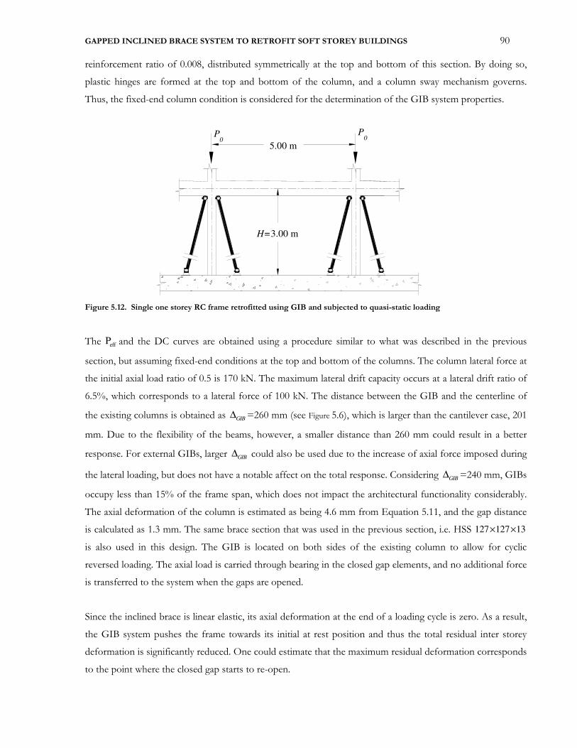
GAPPED INCLINED BRACE SYSTEM TO RETROFIT SOFT STOREY BUILDINGS 90
reinforcement ratio of 0.008, distributed symmetrically at the top and bottom of this section. By doing so,
plastic hinges are formed at the top and bottom of the column, and a column sway mechanism governs.
Thus, the fixed-end column condition is considered for the determination of the GIB system properties.
Figure 5.12. Single one storey RC frame retrofitted using GIB and subjected to quasi-static loading
The effP and the DC curves are obtained using a procedure similar to what was described in the previous
section, but assuming fixed-end conditions at the top and bottom of the columns. The column lateral force at
the initial axial load ratio of 0.5 is 170 kN. The maximum lateral drift capacity occurs at a lateral drift ratio of
6.5%, which corresponds to a lateral force of 100 kN. The distance between the GIB and the centerline of
the existing columns is obtained as GIB∆ =260 mm (see Figure 5.6), which is larger than the cantilever case, 201
mm. Due to the flexibility of the beams, however, a smaller distance than 260 mm could result in a better
response. For external GIBs, larger GIB∆ could also be used due to the increase of axial force imposed during
the lateral loading, but does not have a notable affect on the total response. Considering GIB∆ =240 mm, GIBs
occupy less than 15% of the frame span, which does not impact the architectural functionality considerably.
The axial deformation of the column is estimated as being 4.6 mm from Equation 5.11, and the gap distance
is calculated as 1.3 mm. The same brace section that was used in the previous section, i.e. HSS 127 127 13× ×
is also used in this design. The GIB is located on both sides of the existing column to allow for cyclic
reversed loading. The axial load is carried through bearing in the closed gap elements, and no additional force
is transferred to the system when the gaps are opened.
Since the inclined brace is linear elastic, its axial deformation at the end of a loading cycle is zero. As a result,
the GIB system pushes the frame towards its initial at rest position and thus the total residual inter storey
deformation is significantly reduced. One could estimate that the maximum residual deformation corresponds
to the point where the closed gap starts to re-open.
P0
P 0
H=3.00 m
5.00 m
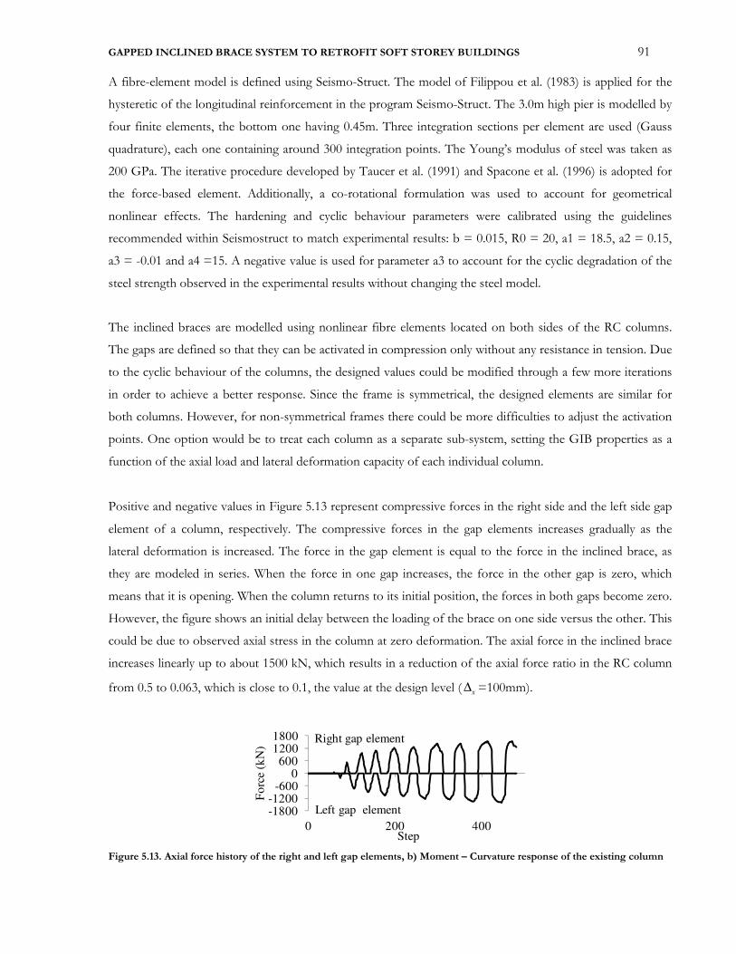
GAPPED INCLINED BRACE SYSTEM TO RETROFIT SOFT STOREY BUILDINGS 91
A fibre-element model is defined using Seismo-Struct. The model of Filippou et al. (1983) is applied for the
hysteretic of the longitudinal reinforcement in the program Seismo-Struct. The 3.0m high pier is modelled by
four finite elements, the bottom one having 0.45m. Three integration sections per element are used (Gauss
quadrature), each one containing around 300 integration points. The Young’s modulus of steel was taken as
200 GPa. The iterative procedure developed by Taucer et al. (1991) and Spacone et al. (1996) is adopted for
the force-based element. Additionally, a co-rotational formulation was used to account for geometrical
nonlinear effects. The hardening and cyclic behaviour parameters were calibrated using the guidelines
recommended within Seismostruct to match experimental results: b = 0.015, R0 = 20, a1 = 18.5, a2 = 0.15,
a3 = -0.01 and a4 =15. A negative value is used for parameter a3 to account for the cyclic degradation of the
steel strength observed in the experimental results without changing the steel model.
The inclined braces are modelled using nonlinear fibre elements located on both sides of the RC columns.
The gaps are defined so that they can be activated in compression only without any resistance in tension. Due
to the cyclic behaviour of the columns, the designed values could be modified through a few more iterations
in order to achieve a better response. Since the frame is symmetrical, the designed elements are similar for
both columns. However, for non-symmetrical frames there could be more difficulties to adjust the activation
points. One option would be to treat each column as a separate sub-system, setting the GIB properties as a
function of the axial load and lateral deformation capacity of each individual column.
Positive and negative values in Figure 5.13 represent compressive forces in the right side and the left side gap
element of a column, respectively. The compressive forces in the gap elements increases gradually as the
lateral deformation is increased. The force in the gap element is equal to the force in the inclined brace, as
they are modeled in series. When the force in one gap increases, the force in the other gap is zero, which
means that it is opening. When the column returns to its initial position, the forces in both gaps become zero.
However, the figure shows an initial delay between the loading of the brace on one side versus the other. This
could be due to observed axial stress in the column at zero deformation. The axial force in the inclined brace
increases linearly up to about 1500 kN, which results in a reduction of the axial force ratio in the RC column
from 0.5 to 0.063, which is close to 0.1, the value at the design level ( x∆ =100mm).
Figure 5.13. Axial force history of the right and left gap elements, b) Moment – Curvature response of the existing column
-1800-1200
-6000
60012001800
0 200 400
Fo
rce
(kN
)
Step
Right gap element
Left gap element
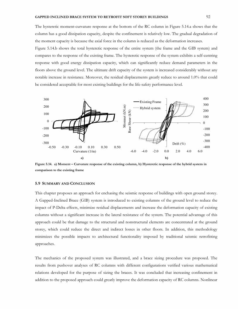
GAPPED INCLINED BRACE SYSTEM TO RETROFIT SOFT STOREY BUILDINGS 92
The hysteretic moment-curvature response at the bottom of the RC column in Figure 5.14.a shows that the
column has a good dissipation capacity, despite the confinement is relatively low. The gradual degradation of
the moment capacity is because the axial force in the column is reduced as the deformation increases.
Figure 5.14.b shows the total hysteretic response of the entire system (the frame and the GIB system) and
compares to the response of the existing frame. The hysteretic response of the system exhibits a self-centring
response with good energy dissipation capacity, which can significantly reduce demand parameters in the
floors above the ground level. The ultimate drift capacity of the system is increased considerably without any
notable increase in resistance. Moreover, the residual displacements greatly reduce to around 1.0% that could
be considered acceptable for most existing buildings for the life-safety performance level.
a) b)
Figure 5.14. a) Moment – Curvature response of the existing column, b) Hysteretic response of the hybrid system in
comparison to the existing frame
5.9 SUMMARY AND CONCLUSION
This chapter proposes an approach for enchasing the seismic response of buildings with open ground storey.
A Gapped-Inclined Brace (GIB) system is introduced to existing columns of the ground level to reduce the
impact of P-Delta effects, minimize residual displacements and increase the deformation capacity of existing
columns without a significant increase in the lateral resistance of the system. The potential advantage of this
approach could be that damage to the structural and nonstructural elements are concentrated at the ground
storey, which could reduce the direct and indirect losses in other floors. In addition, this methodology
minimizes the possible impacts to architectural functionality imposed by traditional seismic retrofitting
approaches.
The mechanics of the proposed system was illustrated, and a brace sizing procedure was proposed. The
results from pushover analyses of RC columns with different configurations verified various mathematical
relations developed for the purpose of sizing the braces. It was concluded that increasing confinement in
addition to the proposed approach could greatly improve the deformation capacity of RC columns. Nonlinear
-300
-200
-100
0
100
200
300
-0.50 -0.30 -0.10 0.10 0.30 0.50
Mo
mn
et (
kN
.m)
Curvature (1/m)
-400
-300
-200
-100
0
100
200
300
400
-6.0 -4.0 -2.0 0.0 2.0 4.0 6.0
Bas
e S
hea
r (k
N)
Drift (%)
Existing Frame
Hybrid system
GAPPED INCLINED BRACE SYSTEM TO RETROFIT SOFT STOREY BUILDINGS 93
quasi-static cyclic analysis of a single span RC frame indicated that the proposed strategy could significantly
improve the hysteretic response of a soft storey frame in terms of energy dissipation capacity and residual
deformation.
The proposed strategy could also be applicable to other types of structures including steel structures, and
bridge piles under high vertical loads. It is, however, recommended that dynamic analyses of case studies be
carried out along with experimental validations to further develop the proposed system and demonstrate its
applicability for the seismic upgrade of such structures.
94
6.SEISMIC RESPONSE OF BUILDINGS USING GIB SYSTEM AND
DESIGN RECOMMENDATIONS
6.1 INTRODUCTION
This chapter presents the seismic responses of the retrofitted soft storey building (using GIB system) that was
studied in Chapter 3. Key aspects related to the numerical modelling of the retrofitted building and the results
from the nonlinear time-history analyses are presented in Section 6.2 to Section 6.5. In Section 6.6 and
Section 6.7, the response of the soft storey building retrofitted using the GIB system is compared with the
existing soft storey building, and the building in which masonry infills are distributed uniformly over the
building height. To investigate the effectiveness of alternate retrofit configurations, different scenarios of GIB
systems is explored in Section 6.8 and 6.9.
6.2 SOFT STOREY CONCEPT FOR MULTI STOREY BUILDINGS
The soft storey concept to reduce the seismic response of buildings by making the first floor to be flexible
dates backs as early as 1920s [Martel 1929]. His study on a four storey building showed that if the stiffness of
the first-story columns are one tenth of that of the floors above it, the response is similar to the one-story
bent. Moreover, he pointed out that the flexible first story could reduce the floor accelerations above the
first storey if the period of the earthquake is less than the free period of the building. This concept
followed by a few researchers [Green 1935; Jacobsen 1938].
In the late of 1960, Fintel and Khan [1969] took first steps to reduce seismic forces using the weak storey
energy dissipated concept. Their proposal was that the first floor should yield at a specific value that cannot
transmit a greater force to the super structure above itself. Chopra et al. [1973] argued that the complexity of
the dynamic earthquake behaviour of multi-storey buildings could invalidate these results. Their parametric
study on an eight storey building concluded that the displacement capacity of the first storey should be very
large. In addition, the yield force and the post yield ratio were required to be very low in order to protect the
super structure effectively.
It should be noted that because the post yield stiffness ratio of the GIB system (existing structural system +
GIB)at the first level is almost zero, it could provide such an effective protection to the super structure.
However, it is recommended to develop a robust methodology to design GIB system for multi-storey
buildings which ensure that storeys above the first floor is protected for desired seismic demands.
6.3 DESIGN CONSIDERATION OF SOFT STOREY BUILDINGS USING THE GIB SYSTEM
Prior to developing a retrofit design solution using a GIB system, it is recommended that the structure first
be assessed using the displacement-based assessment approach of Priestley et al. [2007]. This assessment will
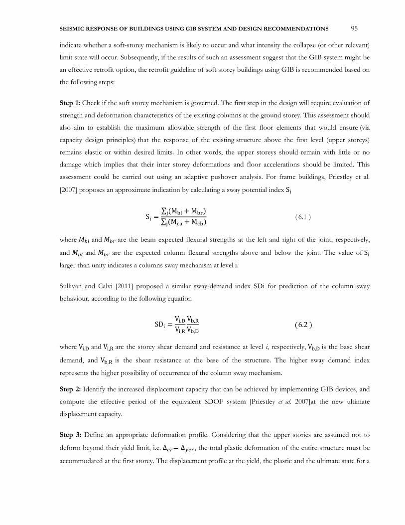
SEISMIC RESPONSE OF BUILDINGS USING GIB SYSTEM AND DESIGN RECOMMENDATIONS 95
indicate whether a soft-storey mechanism is likely to occur and what intensity the collapse (or other relevant)
limit state will occur. Subsequently, if the results of such an assessment suggest that the GIB system might be
an effective retrofit option, the retrofit guideline of soft storey buildings using GIB is recommended based on
the following steps:
Step 1: Check if the soft storey mechanism is governed. The first step in the design will require evaluation of
strength and deformation characteristics of the existing columns at the ground storey. This assessment should
also aim to establish the maximum allowable strength of the first floor elements that would ensure (via
capacity design principles) that the response of the existing structure above the first level (upper storeys)
remains elastic or within desired limits. In other words, the upper storeys should remain with little or no
damage which implies that their inter storey deformations and floor accelerations should be limited. This
assessment could be carried out using an adaptive pushover analysis. For frame buildings, Priestley et al.
[2007] proposes an approximate indication by calculating a sway potential index Sx
Sx = ∑ (M�Û + M�Ü)Ý∑ (M/Ú + M/�)Ý ( 6.1 )
where �]Þ and �]ß are the beam expected flexural strengths at the left and right of the joint, respectively,
and �]Þ and �]ß are the expected column flexural strengths above and below the joint. The value of Sx larger than unity indicates a columns sway mechanism at level i.
Sullivan and Calvi [2011] proposed a similar sway-demand index SDi for prediction of the column sway
behaviour, according to the following equation
SDx = Vx,�Vx,�V�,�V�,� ( 6.2 )
where Vx.� and Vx,� are the storey shear demand and resistance at level i, respectively, V�,� is the base shear
demand, and V�,� is the shear resistance at the base of the structure. The higher sway demand index
represents the higher possibility of occurrence of the column sway mechanism.
Step 2: Identify the increased displacement capacity that can be achieved by implementing GIB devices, and
compute the effective period of the equivalent SDOF system [Priestley et al. 2007]at the new ultimate
displacement capacity.
Step 3: Define an appropriate deformation profile. Considering that the upper stories are assumed not to
deform beyond their yield limit, i.e. ∆½ß= ∆£½ß, the total plastic deformation of the entire structure must be
accommodated at the first storey. The displacement profile at the yield, the plastic and the ultimate state for a
SEISMIC RESPONSE OF BUILDINGS USING GIB SYSTEM AND DESIGN RECOMMENDATIONS 96
2DOF system is shown in Figure 6.1. �½ß , and ∆½ß represents the equivalent mass and the lateral
displacement at the storeys above the first floor.
For an existing building, Ƭ̆ is known. Assuming that the total displacement of the building at a given
hazard level is known (for example by limiting the roof displacement), the first floor displacement is
∆¾= ∆G − ∆£½ß ( 6.3 )
(a) (b) (c)
Figure 6.1. Displacement profile for soft storey frames, a) yield b) plastic, c) Ultimate displacement profile
It could be possible that the deform shape of the structure at the ultimate state is similar to that of the plastic
deformation. This implies that at the ultimate limit state, there is no lateral deformation at the storeys above
the first floor, i.e. ∆¾= ∆G, which simplifies the approach. The displacement ductility capacity o is
calculated as ∆G/∆£¾.
Step 4: Determine the base shear capacity and the effective stiffness. The base shear capacity Và/ is
calculated as
Và/ = °¹�áâ,] + �áã,�¼��z�
/ ¾̂ ( 6.4 )
where �áâ,] and �áã,� are the column moment capacities at the column base and at the beam
centreline at the first level. The equivalent stiffness including P-Delta effects are then given by
Kà = ��*∆G − � (� − ∑ �äå�)¾̂ ( 6.5 )
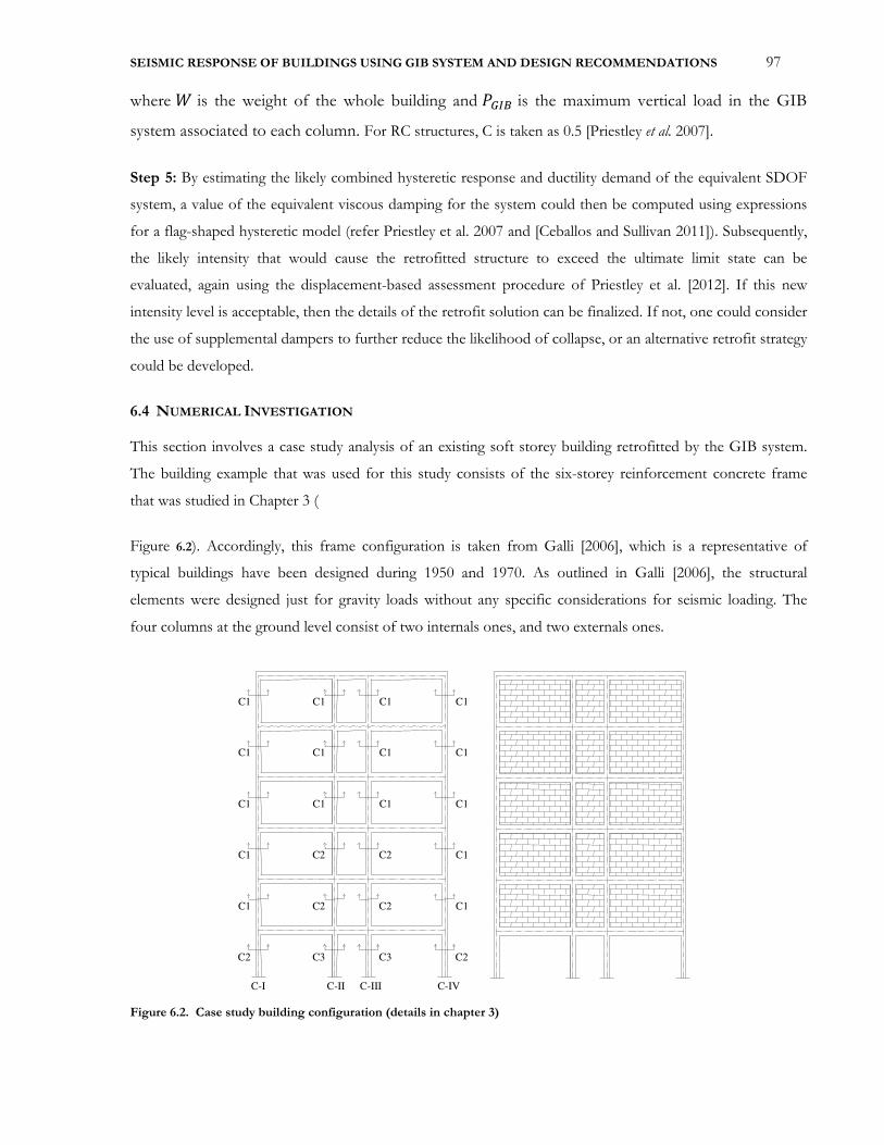
SEISMIC RESPONSE OF BUILDINGS USING GIB SYSTEM AND DESIGN RECOMMENDATIONS 97
where � is the weight of the whole building and �äå� is the maximum vertical load in the GIB
system associated to each column. For RC structures, C is taken as 0.5 [Priestley et al. 2007].
Step 5: By estimating the likely combined hysteretic response and ductility demand of the equivalent SDOF
system, a value of the equivalent viscous damping for the system could then be computed using expressions
for a flag-shaped hysteretic model (refer Priestley et al. 2007 and [Ceballos and Sullivan 2011]). Subsequently,
the likely intensity that would cause the retrofitted structure to exceed the ultimate limit state can be
evaluated, again using the displacement-based assessment procedure of Priestley et al. [2012]. If this new
intensity level is acceptable, then the details of the retrofit solution can be finalized. If not, one could consider
the use of supplemental dampers to further reduce the likelihood of collapse, or an alternative retrofit strategy
could be developed.
6.4 NUMERICAL INVESTIGATION
This section involves a case study analysis of an existing soft storey building retrofitted by the GIB system.
The building example that was used for this study consists of the six-storey reinforcement concrete frame
that was studied in Chapter 3 (
Figure 6.2). Accordingly, this frame configuration is taken from Galli [2006], which is a representative of
typical buildings have been designed during 1950 and 1970. As outlined in Galli [2006], the structural
elements were designed just for gravity loads without any specific considerations for seismic loading. The
four columns at the ground level consist of two internals ones, and two externals ones.
Figure 6.2. Case study building configuration (details in chapter 3)
C2 C3 C3 C2
C1 C2 C2 C1
C1 C2 C2 C1
C1 C1 C1 C1
C1 C1 C1 C1
C1 C1 C1 C1
C-I C-II C-III C-IV

SEISMIC RESPONSE OF BUILDINGS USING GIB SYSTEM AND DESIGN RECOMMENDATIONS 98
The structure is part of a frame system building formed by a series of parallel frames at a distance of 4.5 m
between the centrelines of the columns. The first floor height is 2.75 m, while the other floors have the same
height of 3 m. The frame consists of two 4.5m long identical exterior bays and one interior 2 m bay. Thus,
the frame is symmetric about the vertical axis.
Table 6.1 lists the column details at the first level. Parameters ρ>CFand σ� represent the longitudinal
reinforcement ratio, the confinement factor and the axial load ratio, respectively.
Table 6.1. Column configurations at the open ground level
Column
Type
Dimension Height �] CF
M m %
C1 250 2750 1.29 1.12
C2 300 2750 0.89 1.08
C3 350 2750 0.83 1.07
To determine the most effective use of the system, different implementation configurations of the GIB are
studied, as shown in Figure 6.3:
i) Configuration 1 (Figure 6.3.a): the properties of the GIB system are defined without considering the
changes in the axial load during the ground motion history. This configuration is referred to as GIB-1
variant.
ii) Configuration 2 (Figure 6.3.b): the increase and decrease in the column axial loads due to lateral loads is
considered. As such, GIBs that are at the exterior side of the exterior columns are designed for stronger
actions, while GIBs that are at the interior side of the exterior columns are eliminated, because their
actions are not significant. This configuration is referred to as GIB-2 variant.
iii) Configuration 3 (Figure 6.3.c): The number of GIBs in the interior columns are also decreased. As such,
GIBs that are at the interior side of the interior columns are eliminated. The aim is to reduce the cost
and to increase the architectural functionality. This configuration is referred to as GIB-3 variant.
The response of the retrofitted building is compared with the existing soft storey building, and the building in
which masonry infills are distributed uniformly over the building height (full infill). Finally, the effect of
supplemental damping on the response of the GIB-3 variatn will be explored numerically.
6.5 GIB- 1 VARIANT
As a first step, the GIB system associated with each column is designed based on the aforementioned
procedure which neglects the axial loads while the effect of the varying axial load will be further discussed
later. This configuration is shown in Figure 6.3 , which is referred as GIB1 Variant. As such, the GIBs that
corresponds to the exterior columns, i.e., GIB-1L, GIB-1R, GIB-4L, GIB-4R, are designed for the same
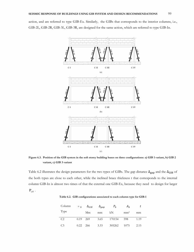
SEISMIC RESPONSE OF BUILDINGS USING GIB SYSTEM AND DESIGN RECOMMENDATIONS 99
action, and are referred to type GIB-Ex. Similarly, the GIBs that corresponds to the interior columns, i.e.,
GIB-2L, GIB-2R, GIB-3L, GIB-3R, are designed for the same action, which are referred to type GIB-In.
Figure 6.3. Position of the GIB system in the soft storey building bases on three configurations: a) GIB 1 variant, b) GIB 2
variant, c) GIB 3 variant
Table 6.2 illustrates the design parameters for the two types of GIBs. The gap distance ∆rÚ3 and the ∆æçà of
the both types are close to each other, while the inclined brace thickness t that corresponds to the internal
column GIB-In is almost two times of that the external one GIB-Ex, because they need to design for larger
effP .
Table 6.2. GIB configurations associated to each column type for GIB-1
Column
Type
σ� ∆äå� ∆|�, �] X] ! Mm mm kN mm2 mm
C2 0.19 269 3.65 170154 598 1.19
C3 0.22 266 3.33 305262 1075 2.15
C-I C-II C-III C-IV
GIB
-3L G
IB-3
R
GIB
-2L
GIB
-2R
GIB
-1L
GIB
-1R
GIB
-4L
GIB
-4R
GIB
-3L G
IB-3
R
GIB
-2L
GIB
-2R
GIB
-1L
GIB
-4R
C-I C-II C-III C-IV
GIB
-3R
GIB
-2L
GIB
-1L
GIB
-4R
C-I C-II C-III C-IV
(a)
(b)
(c)
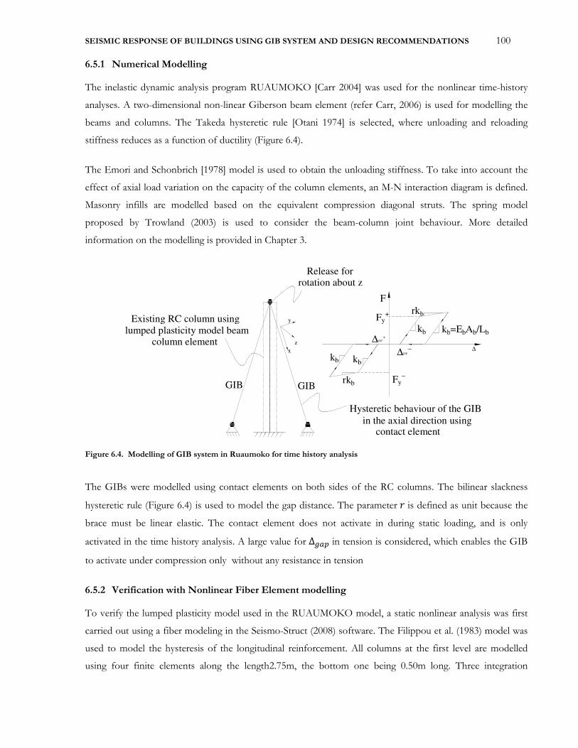
SEISMIC RESPONSE OF BUILDINGS USING GIB SYSTEM AND DESIGN RECOMMENDATIONS 100
6.5.1 Numerical Modelling
The inelastic dynamic analysis program RUAUMOKO [Carr 2004] was used for the nonlinear time-history
analyses. A two-dimensional non-linear Giberson beam element (refer Carr, 2006) is used for modelling the
beams and columns. The Takeda hysteretic rule [Otani 1974] is selected, where unloading and reloading
stiffness reduces as a function of ductility (Figure 6.4).
The Emori and Schonbrich [1978] model is used to obtain the unloading stiffness. To take into account the
effect of axial load variation on the capacity of the column elements, an M-N interaction diagram is defined.
Masonry infills are modelled based on the equivalent compression diagonal struts. The spring model
proposed by Trowland (2003) is used to consider the beam-column joint behaviour. More detailed
information on the modelling is provided in Chapter 3.
Figure 6.4. Modelling of GIB system in Ruaumoko for time history analysis
The GIBs were modelled using contact elements on both sides of the RC columns. The bilinear slackness
hysteretic rule (Figure 6.4) is used to model the gap distance. The parameter � is defined as unit because the
brace must be linear elastic. The contact element does not activate in during static loading, and is only
activated in the time history analysis. A large value for ∆|�, in tension is considered, which enables the GIB
to activate under compression only without any resistance in tension
6.5.2 Verification with Nonlinear Fiber Element modelling
To verify the lumped plasticity model used in the RUAUMOKO model, a static nonlinear analysis was first
carried out using a fiber modeling in the Seismo-Struct (2008) software. The Filippou et al. (1983) model was
used to model the hysteresis of the longitudinal reinforcement. All columns at the first level are modelled
using four finite elements along the length2.75m, the bottom one being 0.50m long. Three integration
y
z x
F
F y+
F y −
∆
Hysteretic behaviour of the GIB
in the axial direction usingcontact element
Release for rotation about z
kb=Eb A b /Lb
rkb
kb kb
∆ gap+
∆gap−
kb
rk b Existing RC column using
lumped plasticity model beamcolumn element
GIBGIB

SEISMIC RESPONSE OF BUILDINGS USING GIB SYSTEM AND DESIGN RECOMMENDATIONS 101
sections per element are used (Gauss quadrature), each one containing around 250 integration points. The
Young’s modulus of steel was taken as 200 GPa.
The Mander model [Mander et al. 1988] was used to evaluate the constitutive relations for the confined and
the unconfined concrete under compression. To incorporate the constitutive relations for reinforcement steel,
the model proposed by King et al. [1986] was adopted.
The strain at maximum stress for unconfined concrete was assumed to be 0.002. The ultimate concrete strain
was governed by the core crushing limit state proposed by Kowalsky [2000], and the ultimate tensile strain of
the reinforcement was assumed to be 12%.
The iterative procedure developed by Taucer et al. (1991) and Spacone et al. (1996) is adopted for the force-
based element. Additionally, a co-rotational formulation was used to account for geometrical nonlinear
effects. The hardening and cyclic behaviour parameters were calibrated using the guidelines recommended
within Seismostruct to match experimental results: b = 0.015, R0 = 20, a1 = 18.5, a2 = 0.15, a3 = -0.01 and
a4 =15. A negative value is used for parameter a3 to account for the cyclic degradation of the steel strength
observed in the experimental results without changing the steel model.
The four-node masonry panel element, which is initially developed by programmed by Crisafulli [1997], is
used in SeismoStruct for modelling the nonlinear response of infill panels (Figure 6.5). Each panel is
represented by six strut members; each diagonal direction features two parallel struts to carry axial loads
across two opposite diagonal corners and a third one to carry the shear from the top to the bottom of the
panel. This latter strut only acts across the diagonal that is on compression, hence its "activation" depends on
the deformation of the panel.
To consider the actual points of contact between the frame and the infill panel, four internal nodes are
employed. These four nodes corresponds for the width and height of the columns and beams, respectivel. In
addition, four dummy nodes are introduced to consider the contact length between the frame and the infill
panel. The properties of the masonry infill and the related assumptions are found in Chpater3.
It should be noted that this model incorporates only the most frequent of modes of failure, which could
predict the exact behaviour of the structure. In addition, all dispersion of mechanical properties of masonry
could increase uncertainty of infills characteristics and affects the global response of the structure.
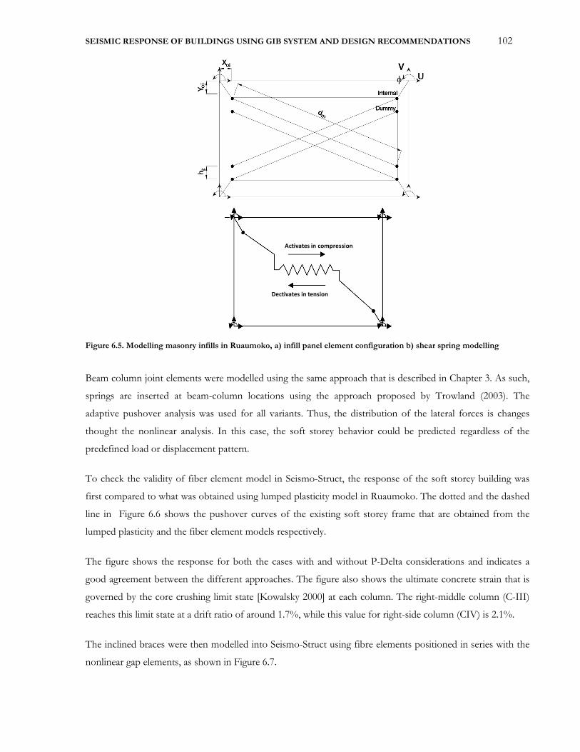
SEISMIC RESPONSE OF BUILDINGS USING GIB SYSTEM AND DESIGN RECOMMENDATIONS 102
Figure 6.5. Modelling masonry infills in Ruaumoko, a) infill panel element configuration b) shear spring modelling
Beam column joint elements were modelled using the same approach that is described in Chapter 3. As such,
springs are inserted at beam-column locations using the approach proposed by Trowland (2003). The
adaptive pushover analysis was used for all variants. Thus, the distribution of the lateral forces is changes
thought the nonlinear analysis. In this case, the soft storey behavior could be predicted regardless of the
predefined load or displacement pattern.
To check the validity of fiber element model in Seismo-Struct, the response of the soft storey building was
first compared to what was obtained using lumped plasticity model in Ruaumoko. The dotted and the dashed
line in Figure 6.6 shows the pushover curves of the existing soft storey frame that are obtained from the
lumped plasticity and the fiber element models respectively.
The figure shows the response for both the cases with and without P-Delta considerations and indicates a
good agreement between the different approaches. The figure also shows the ultimate concrete strain that is
governed by the core crushing limit state [Kowalsky 2000] at each column. The right-middle column (C-III)
reaches this limit state at a drift ratio of around 1.7%, while this value for right-side column (CIV) is 2.1%.
The inclined braces were then modelled into Seismo-Struct using fibre elements positioned in series with the
nonlinear gap elements, as shown in Figure 6.7.
Activates in compression
Dectivates in tension
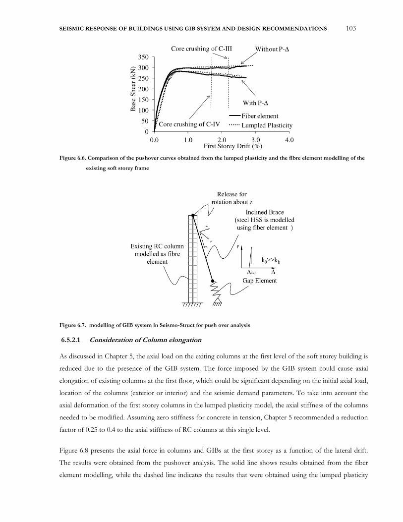
SEISMIC RESPONSE OF BUILDINGS USING GIB SYSTEM AND DESIGN RECOMMENDATIONS 103
Figure 6.6. Comparison of the pushover curves obtained from the lumped plasticity and the fibre element modelling of the
existing soft storey frame
Figure 6.7. modelling of GIB system in Seismo-Struct for push over analysis
6.5.2.1 Consideration of Column elongation
As discussed in Chapter 5, the axial load on the exiting columns at the first level of the soft storey building is
reduced due to the presence of the GIB system. The force imposed by the GIB system could cause axial
elongation of existing columns at the first floor, which could be significant depending on the initial axial load,
location of the columns (exterior or interior) and the seismic demand parameters. To take into account the
axial deformation of the first storey columns in the lumped plasticity model, the axial stiffness of the columns
needed to be modified. Assuming zero stiffness for concrete in tension, Chapter 5 recommended a reduction
factor of 0.25 to 0.4 to the axial stiffness of RC columns at this single level.
Figure 6.8 presents the axial force in columns and GIBs at the first storey as a function of the lateral drift.
The results were obtained from the pushover analysis. The solid line shows results obtained from the fiber
element modelling, while the dashed line indicates the results that were obtained using the lumped plasticity
0
50
100
150
200
250
300
350
0.0 1.0 2.0 3.0 4.0B
ase
Sh
ear
(kN
)
First Storey Drift (%)
Fiber element
Lumpled Plasticity
With P-∆
Without P-∆
Core crushing of C-IV
Core crushing of C-III
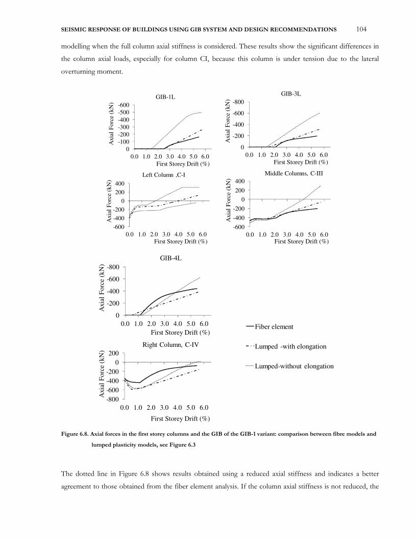
SEISMIC RESPONSE OF BUILDINGS USING GIB SYSTEM AND DESIGN RECOMMENDATIONS 104
modelling when the full column axial stiffness is considered. These results show the significant differences in
the column axial loads, especially for column CI, because this column is under tension due to the lateral
overturning moment.
Figure 6.8. Axial forces in the first storey columns and the GIB of the GIB-1 variant: comparison between fibre models and
lumped plasticity models, see Figure 6.3
The dotted line in Figure 6.8 shows results obtained using a reduced axial stiffness and indicates a better
agreement to those obtained from the fiber element analysis. If the column axial stiffness is not reduced, the
-600
-500
-400
-300
-200
-100
0
0.0 1.0 2.0 3.0 4.0 5.0 6.0
Axia
l F
orc
e (k
N)
First Storey Drift (%)
Axia
l F
orc
e (k
N)
-600
-400
-200
0
200
400
0.0 1.0 2.0 3.0 4.0 5.0 6.0
Axia
l F
orc
e (k
N)
First Storey Drift (%)
Axia
l F
orc
e (k
N)
GIB-1L GIB
Left Column ,C-I Middle Columns, C
-800
-600
-400
-200
0
0.0 1.0 2.0 3.0 4.0 5.0 6.0
Axia
l F
orc
e (k
N)
First Storey Drift (%)
-600
-400
-200
0
200
400
0.0 1.0 2.0 3.0 4.0 5.0 6.0A
xia
l F
orc
e (k
N)
First Storey Drift (%)
1L GIB-3L
I Middle Columns, C-III Right Colum
-800
-600
-400
-200
0
0.0 1.0 2.0 3.0 4.0 5.0 6.0
Axia
l F
orc
e (k
N)
First Storey Drift (%)
-800
-600
-400
-200
0
200
0.0 1.0 2.0 3.0 4.0 5.0 6.0
Axia
l F
orc
e (k
N)
First Storey Drift (%)
3L GIB-4L
III Right Column, C-IV
Fiber element
Lumped -with elongation
Lumped-without elongation
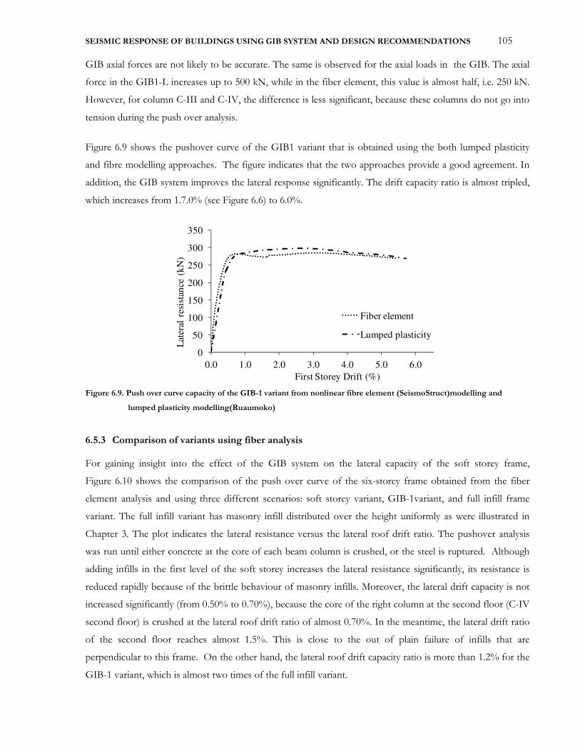
SEISMIC RESPONSE OF BUILDINGS USING GIB SYSTEM AND DESIGN RECOMMENDATIONS 105
GIB axial forces are not likely to be accurate. The same is observed for the axial loads in the GIB. The axial
force in the GIB1-L increases up to 500 kN, while in the fiber element, this value is almost half, i.e. 250 kN.
However, for column C-III and C-IV, the difference is less significant, because these columns do not go into
tension during the push over analysis.
Figure 6.9 shows the pushover curve of the GIB1 variant that is obtained using the both lumped plasticity
and fibre modelling approaches. The figure indicates that the two approaches provide a good agreement. In
addition, the GIB system improves the lateral response significantly. The drift capacity ratio is almost tripled,
which increases from 1.7.0% (see Figure 6.6) to 6.0%.
Figure 6.9. Push over curve capacity of the GIB-1 variant from nonlinear fibre element (SeismoStruct)modelling and
lumped plasticity modelling(Ruaumoko)
6.5.3 Comparison of variants using fiber analysis
For gaining insight into the effect of the GIB system on the lateral capacity of the soft storey frame,
Figure 6.10 shows the comparison of the push over curve of the six-storey frame obtained from the fiber
element analysis and using three different scenarios: soft storey variant, GIB-1variant, and full infill frame
variant. The full infill variant has masonry infill distributed over the height uniformly as were illustrated in
Chapter 3. The plot indicates the lateral resistance versus the lateral roof drift ratio. The pushover analysis
was run until either concrete at the core of each beam column is crushed, or the steel is ruptured. Although
adding infills in the first level of the soft storey increases the lateral resistance significantly, its resistance is
reduced rapidly because of the brittle behaviour of masonry infills. Moreover, the lateral drift capacity is not
increased significantly (from 0.50% to 0.70%), because the core of the right column at the second floor (C-IV
second floor) is crushed at the lateral roof drift ratio of almost 0.70%. In the meantime, the lateral drift ratio
of the second floor reaches almost 1.5%. This is close to the out of plain failure of infills that are
perpendicular to this frame. On the other hand, the lateral roof drift capacity ratio is more than 1.2% for the
GIB-1 variant, which is almost two times of the full infill variant.
0
50
100
150
200
250
300
350
0.0 1.0 2.0 3.0 4.0 5.0 6.0
Lat
eral
res
ista
nce
(k
N)
First Storey Drift (%)
Fiber element
Lumped plasticity

SEISMIC RESPONSE OF BUILDINGS USING GIB SYSTEM AND DESIGN RECOMMENDATIONS 106
Figure 6.10. Push over curve capacity for the six-storey frame buildings a) Full infill, b) Partial infill, c) GIB-1 variant
Figure 6.11 depicts the material limit states pattern in the beam and the column elements of the three
variants. These damage states are obtained at the ultimate drift capacity of each variant, which was shown in
Figure 6.10. The limit states are illustrated at the bottom of this figure, which are separated by different
colors. The damage pattern for the full infill case is much more evenly distributed. Plastic hinges are mainly
formed in the second. Concrete core strain at the columns of the second floors exceeds its ultimate capacity,
i.e. 2.0%, and in the third and the fourth floors, some elements yield.
For the partial infill case, all damage is concentrated in the first floor only. Plastic hinges form in all columns
at the first level at the lateral roof drift ratio of 0.50%, which corresponds to the lateral first storey drift ratio
of 1.7% that were previously shown in Figure 6.6 . As discussed, at this drift ratio, columns CIII and CIV
reached the core crushing limit states.
However, when the building is retrofitted using the GIB system (GIB-1 variant), the roof drift capacity
increases to 1.2%, while all damages are still accumulated at the first level of the soft storey building. Before
this drift ratio, none of the beams and columns of the first floor reach their ultimate limit states before, which
is core crush of concrete, rebar buckling or steel rupture. The first floor displacement and the roof
displacement at this level are 0.21m and 0.17m, respectively, which denotes that the drift ratio at the floors
above the first floor is very low, and all are in the elastic range. The figure denotes that at this roof drift ratio,
neither cover spalls or nor steels yields in beams and columns in all the storeys above the first floor.
6.5.4 Results from Nonlinear Time History Analyses
Time history analyses are also carried out using ten recorded horizontal accelerograms selected as part of the
DISTEEL project [Maley et al. 2013]. The record set consists of 10 records that are scaled to be compatible
with Eurocode 8 spectrum [CEN 2004] for soil type C and a corner period Td = 8s.
0
200
400
600
800
1000
1200
0.0 0.2 0.4 0.6 0.8 1.0 1.2
Lat
eral
res
ista
nce
(kN
)
Roof Drift (%)
Full infill variantSoft storey varinatGIB-1 variant
First floor: core crushing of C-IV
First floorSteel
rupture of C-ISecon floor: Core crushing of C-IV
+ potential out of plain failure of infills
in prependicular frames
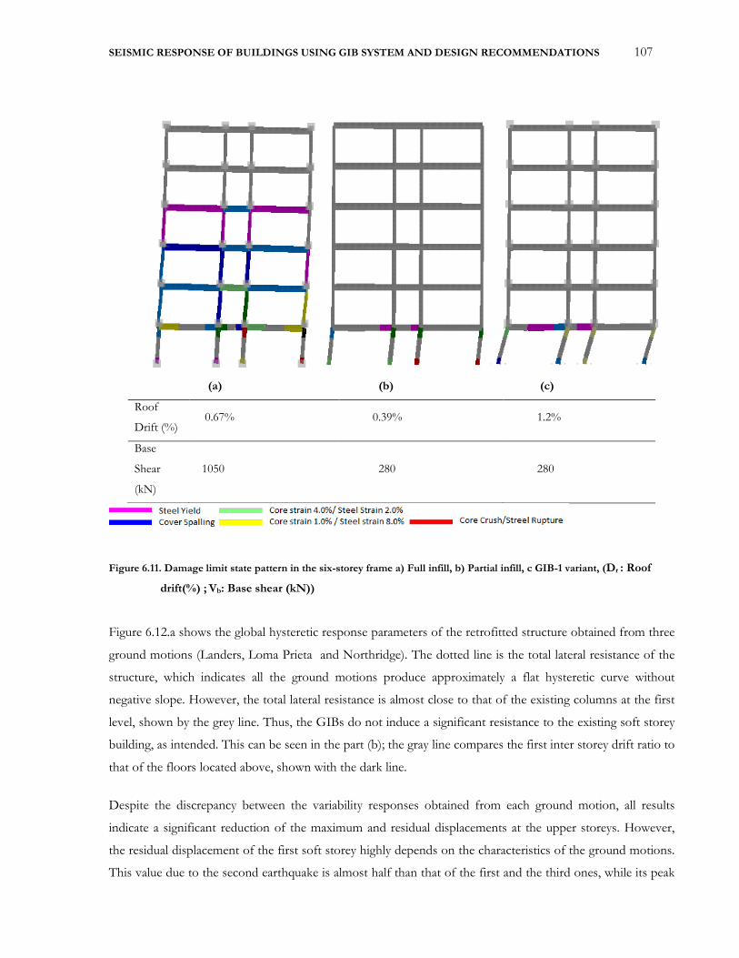
SEISMIC RESPONSE OF BUILDINGS USING GIB SYSTEM AND DESIGN RECOMMENDATIONS 107
(a) (b) (c)
Roof
Drift (%) 0.67% 0.39% 1.2%
Base
Shear
(kN)
1050 280 280
Figure 6.11. Damage limit state pattern in the six-storey frame a) Full infill, b) Partial infill, c GIB-1 variant, (Dr : Roof
drift(%) ; Vb: Base shear (kN))
Figure 6.12.a shows the global hysteretic response parameters of the retrofitted structure obtained from three
ground motions (Landers, Loma Prieta and Northridge). The dotted line is the total lateral resistance of the
structure, which indicates all the ground motions produce approximately a flat hysteretic curve without
negative slope. However, the total lateral resistance is almost close to that of the existing columns at the first
level, shown by the grey line. Thus, the GIBs do not induce a significant resistance to the existing soft storey
building, as intended. This can be seen in the part (b); the gray line compares the first inter storey drift ratio to
that of the floors located above, shown with the dark line.
Despite the discrepancy between the variability responses obtained from each ground motion, all results
indicate a significant reduction of the maximum and residual displacements at the upper storeys. However,
the residual displacement of the first soft storey highly depends on the characteristics of the ground motions.
This value due to the second earthquake is almost half than that of the first and the third ones, while its peak
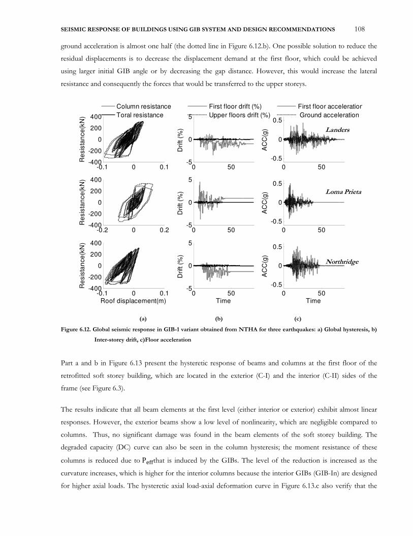
SEISMIC RESPONSE OF BUILDINGS USING GIB SYSTEM AND DESIGN RECOMMENDATIONS 108
ground acceleration is almost one half (the dotted line in Figure 6.12.b). One possible solution to reduce the
residual displacements is to decrease the displacement demand at the first floor, which could be achieved
using larger initial GIB angle or by decreasing the gap distance. However, this would increase the lateral
resistance and consequently the forces that would be transferred to the upper storeys.
(a) (b) (c)
Figure 6.12. Global seismic response in GIB-1 variant obtained from NTHA for three earthquakes: a) Global hysteresis, b)
Inter-storey drift, c)Floor acceleration
Part a and b in Figure 6.13 present the hysteretic response of beams and columns at the first floor of the
retrofitted soft storey building, which are located in the exterior (C-I) and the interior (C-II) sides of the
frame (see Figure 6.3).
The results indicate that all beam elements at the first level (either interior or exterior) exhibit almost linear
responses. However, the exterior beams show a low level of nonlinearity, which are negligible compared to
columns. Thus, no significant damage was found in the beam elements of the soft storey building. The
degraded capacity (DC) curve can also be seen in the column hysteresis; the moment resistance of these
columns is reduced due to PÃÄÄthat is induced by the GIBs. The level of the reduction is increased as the
curvature increases, which is higher for the interior columns because the interior GIBs (GIB-In) are designed
for higher axial loads. The hysteretic axial load-axial deformation curve in Figure 6.13.c also verify that the
-0.1 0 0.1-400
-200
0
200
400
Re
sis
tan
ce
(kN
)
0 50-5
0
5
Drift (
%)
0 50
-0.5
0
0.5
AC
C(g
)
-0.2 0 0.2-400
-200
0
200
400
Re
sis
tan
ce
(kN
)
0 50-5
0
5D
rift (
%)
0 50
-0.5
0
0.5
AC
C(g
)
-0.1 0 0.1-400
-200
0
200
400
Re
sis
tan
ce
(kN
)
Roof displacement(m)
0 50-5
0
5
Drift (
%)
Time
0 50
-0.5
0
0.5
AC
C(g
)
Time
First floor acceleration
Ground acceleration
Column resistance
Toral resistance
First floor drift (%)
Upper floors drift (%)
Landers
Loma Prieta
Northridge

SEISMIC RESPONSE OF BUILDINGS USING GIB SYSTEM AND DESIGN RECOMMENDATIONS 109
axial load in interior GIBs (GIB-In, the dark line) is larger than that of the exterior ones (GIB-Ex, the gray
line). In addition, the stiffness of GIB-In is larger than that of GIB-Ex. The gap distance for both the interior
and exterior GIBs is almost the same, and is 3.65 mm.
(a) (b) (c)
Figure 6.13. Element hysteretic responses in GIB-1 variant: a) Moment-curvature of exterior Beams and columns, b)
Moment-curvature of interior Beams and columns c) Axial GIBs hysteresis
Figure 6.14 shows the time history of the axial loads of the first storey elements (Columns and GIBs) at
different sides of the frame under the three earthquakes at the design (DBD) level. The axial force of the
middle columns decreases from 500 kN to almost 190 kN, which result in a maximum axial load of 310kN in
the GIB-In, which is less than for the GIB-Ex. For the columns at the right side of the building, the
maximum axial compressive load is even increased from 350 kN to almost 600 kN. On the other hand, the
column in the left side goes to tension (maximum axial force 210 kN). The tension in these columns could
decrease their lateral displacement capacity. Thus, using the GIB-1R and GIB-4L could have even negative
effects on the lateral capacity of columns at the first floor. As a result, if these GIBs are eliminated, and
instead, GIB-1L and GIB-4R are designed for stronger actions, the seismic response of the retrofitted
building could be improved. Section 6.9 will investigate this scenario.
-0.2 -0.1 0 0.1
-100
0
100
Mo
me
nt(
kN
.m)
Beam and Column (Exterior)
-0.2 -0.1 0 0.1
-100
0
100
Mo
me
nt(
kN
.m)
Beam and column (Interior)
-0.01 0 0.01
-200
0
200
400
Axia
l fo
rce
(kN
)
GIB
-0.2 -0.1 0 0.1
-100
0
100
Mo
me
nt(
kN
.m)
-0.2 -0.1 0 0.1
-100
0
100M
om
en
t(kN
.m)
-0.01 0 0.01
-200
0
200
400
Axia
l fo
rce
(kN
)
-0.2 -0.1 0 0.1
-100
0
100
Mo
me
nt(
kN
.m)
Curvature (1/m)
-0.2 -0.1 0 0.1
-100
0
100
Mo
me
nt(
kN
.m)
Curvature (1/m)
-0.01 0 0.01
-200
0
200
400
Axia
l fo
rce
(kN
)
GIB Elongation (m)Column Beam Exterior Interior
Landers
Loma Prieta
Northridge
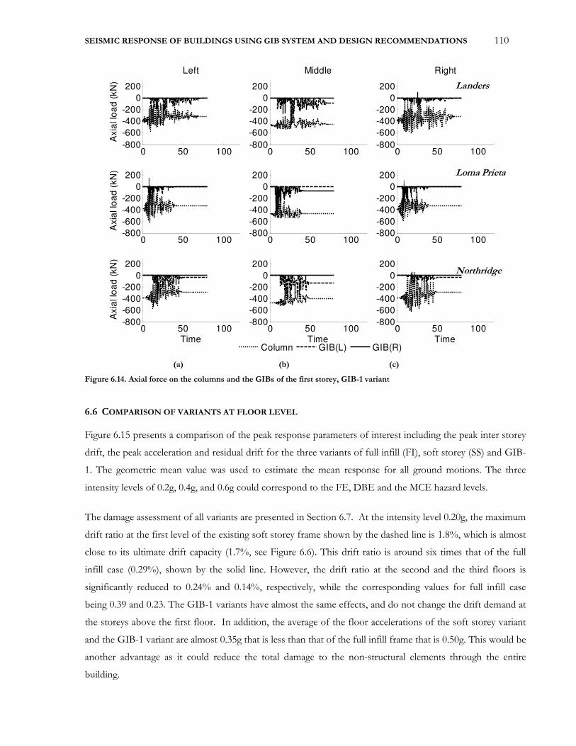
SEISMIC RESPONSE OF BUILDINGS USING GIB SYSTEM AND DESIGN RECOMMENDATIONS 110
(a) (b) (c)
Figure 6.14. Axial force on the columns and the GIBs of the first storey, GIB-1 variant
6.6 COMPARISON OF VARIANTS AT FLOOR LEVEL
Figure 6.15 presents a comparison of the peak response parameters of interest including the peak inter storey
drift, the peak acceleration and residual drift for the three variants of full infill (FI), soft storey (SS) and GIB-
1. The geometric mean value was used to estimate the mean response for all ground motions. The three
intensity levels of 0.2g, 0.4g, and 0.6g could correspond to the FE, DBE and the MCE hazard levels.
The damage assessment of all variants are presented in Section 6.7. At the intensity level 0.20g, the maximum
drift ratio at the first level of the existing soft storey frame shown by the dashed line is 1.8%, which is almost
close to its ultimate drift capacity (1.7%, see Figure 6.6). This drift ratio is around six times that of the full
infill case (0.29%), shown by the solid line. However, the drift ratio at the second and the third floors is
significantly reduced to 0.24% and 0.14%, respectively, while the corresponding values for full infill case
being 0.39 and 0.23. The GIB-1 variants have almost the same effects, and do not change the drift demand at
the storeys above the first floor. In addition, the average of the floor accelerations of the soft storey variant
and the GIB-1 variant are almost 0.35g that is less than that of the full infill frame that is 0.50g. This would be
another advantage as it could reduce the total damage to the non-structural elements through the entire
building.
0 50 100-800
-600
-400
-200
0
200
Axia
l lo
ad
(kN
)
Left
0 50 100-800
-600
-400
-200
0
200
Middle
0 50 100-800
-600
-400
-200
0
200
Right
0 50 100-800
-600
-400
-200
0
200
Axia
l lo
ad
(kN
)
0 50 100-800
-600
-400
-200
0
200
0 50 100-800
-600
-400
-200
0
200
0 50 100-800
-600
-400
-200
0
200
Axia
l lo
ad
(kN
)
Time0 50 100
-800
-600
-400
-200
0
200
Time0 50 100
-800
-600
-400
-200
0
200
Time
Column GIB(L) GIB(R)
Landers
Loma Prieta
Northridge
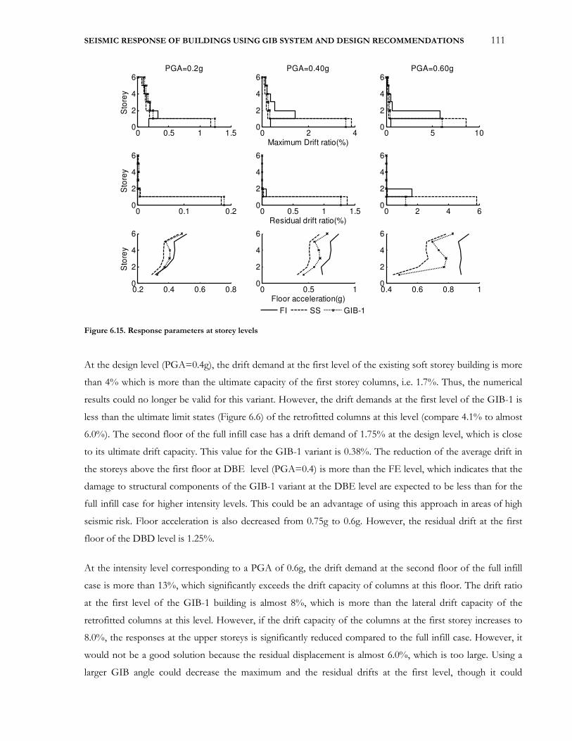
SEISMIC RESPONSE OF BUILDINGS USING GIB SYSTEM AND DESIGN RECOMMENDATIONS 111
Figure 6.15. Response parameters at storey levels
At the design level (PGA=0.4g), the drift demand at the first level of the existing soft storey building is more
than 4% which is more than the ultimate capacity of the first storey columns, i.e. 1.7%. Thus, the numerical
results could no longer be valid for this variant. However, the drift demands at the first level of the GIB-1 is
less than the ultimate limit states (Figure 6.6) of the retrofitted columns at this level (compare 4.1% to almost
6.0%). The second floor of the full infill case has a drift demand of 1.75% at the design level, which is close
to its ultimate drift capacity. This value for the GIB-1 variant is 0.38%. The reduction of the average drift in
the storeys above the first floor at DBE level (PGA=0.4) is more than the FE level, which indicates that the
damage to structural components of the GIB-1 variant at the DBE level are expected to be less than for the
full infill case for higher intensity levels. This could be an advantage of using this approach in areas of high
seismic risk. Floor acceleration is also decreased from 0.75g to 0.6g. However, the residual drift at the first
floor of the DBD level is 1.25%.
At the intensity level corresponding to a PGA of 0.6g, the drift demand at the second floor of the full infill
case is more than 13%, which significantly exceeds the drift capacity of columns at this floor. The drift ratio
at the first level of the GIB-1 building is almost 8%, which is more than the lateral drift capacity of the
retrofitted columns at this level. However, if the drift capacity of the columns at the first storey increases to
8.0%, the responses at the upper storeys is significantly reduced compared to the full infill case. However, it
would not be a good solution because the residual displacement is almost 6.0%, which is too large. Using a
larger GIB angle could decrease the maximum and the residual drifts at the first level, though it could
0 0.5 1 1.50
2
4
6PGA=0.2g
Sto
rey
0 0.1 0.20
2
4
6
Sto
rey
0.2 0.4 0.6 0.80
2
4
6
Sto
rey
0 2 40
2
4
6PGA=0.40g
Maximum Drift ratio(%)
0 0.5 1 1.50
2
4
6
Residual drift ratio(%)
0 0.5 10
2
4
6
Floor acceleration(g)
0 5 100
2
4
6PGA=0.60g
0 2 4 60
2
4
6
0.4 0.6 0.8 10
2
4
6
FI SS GIB-1
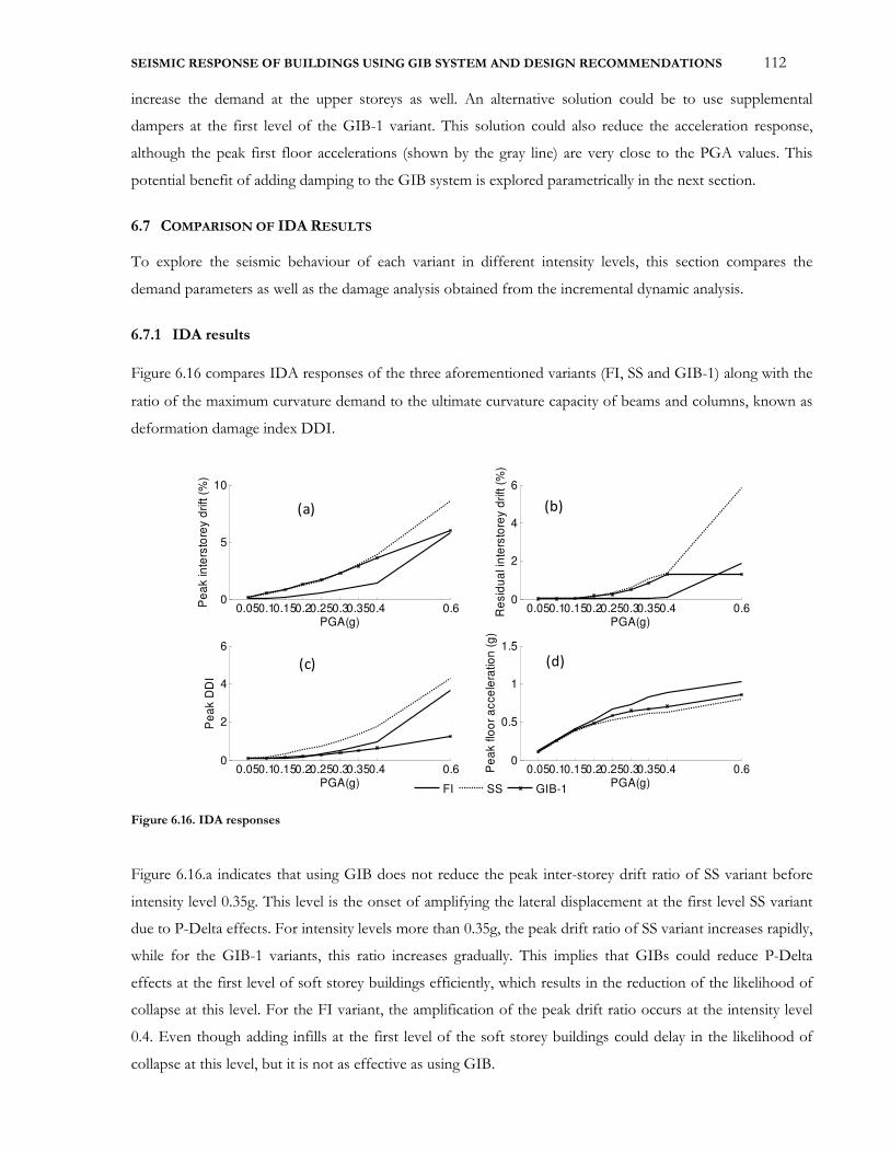
SEISMIC RESPONSE OF BUILDINGS USING GIB SYSTEM AND DESIGN RECOMMENDATIONS 112
increase the demand at the upper storeys as well. An alternative solution could be to use supplemental
dampers at the first level of the GIB-1 variant. This solution could also reduce the acceleration response,
although the peak first floor accelerations (shown by the gray line) are very close to the PGA values. This
potential benefit of adding damping to the GIB system is explored parametrically in the next section.
6.7 COMPARISON OF IDA RESULTS
To explore the seismic behaviour of each variant in different intensity levels, this section compares the
demand parameters as well as the damage analysis obtained from the incremental dynamic analysis.
6.7.1 IDA results
Figure 6.16 compares IDA responses of the three aforementioned variants (FI, SS and GIB-1) along with the
ratio of the maximum curvature demand to the ultimate curvature capacity of beams and columns, known as
deformation damage index DDI.
Figure 6.16. IDA responses
Figure 6.16.a indicates that using GIB does not reduce the peak inter-storey drift ratio of SS variant before
intensity level 0.35g. This level is the onset of amplifying the lateral displacement at the first level SS variant
due to P-Delta effects. For intensity levels more than 0.35g, the peak drift ratio of SS variant increases rapidly,
while for the GIB-1 variants, this ratio increases gradually. This implies that GIBs could reduce P-Delta
effects at the first level of soft storey buildings efficiently, which results in the reduction of the likelihood of
collapse at this level. For the FI variant, the amplification of the peak drift ratio occurs at the intensity level
0.4. Even though adding infills at the first level of the soft storey buildings could delay in the likelihood of
collapse at this level, but it is not as effective as using GIB.
0.050.10.150.20.250.30.350.4 0.60
5
10
Pe
ak in
ters
tore
y d
rift (
%)
PGA(g)0.050.10.150.20.250.30.350.4 0.6
0
2
4
6
Re
sid
ua
l in
ters
tore
y d
rift (
%)
PGA(g)
0.050.10.150.20.250.30.350.4 0.60
0.5
1
1.5
Pe
ak flo
or
acce
lera
tion
(g
)
PGA(g)0.050.10.150.20.250.30.350.4 0.6
0
2
4
6
Pe
ak D
DI
PGA(g)
FI SS GIB-1
(a) (b)
(c) (d)
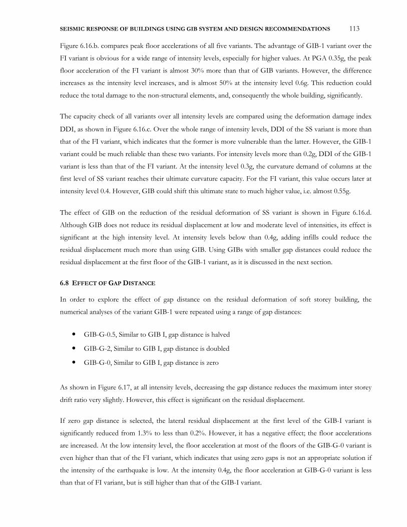
SEISMIC RESPONSE OF BUILDINGS USING GIB SYSTEM AND DESIGN RECOMMENDATIONS 113
Figure 6.16.b. compares peak floor accelerations of all five variants. The advantage of GIB-1 variant over the
FI variant is obvious for a wide range of intensity levels, especially for higher values. At PGA 0.35g, the peak
floor acceleration of the FI variant is almost 30% more than that of GIB variants. However, the difference
increases as the intensity level increases, and is almost 50% at the intensity level 0.6g. This reduction could
reduce the total damage to the non-structural elements, and, consequently the whole building, significantly.
The capacity check of all variants over all intensity levels are compared using the deformation damage index
DDI, as shown in Figure 6.16.c. Over the whole range of intensity levels, DDI of the SS variant is more than
that of the FI variant, which indicates that the former is more vulnerable than the latter. However, the GIB-1
variant could be much reliable than these two variants. For intensity levels more than 0.2g, DDI of the GIB-1
variant is less than that of the FI variant. At the intensity level 0.3g, the curvature demand of columns at the
first level of SS variant reaches their ultimate curvature capacity. For the FI variant, this value occurs later at
intensity level 0.4. However, GIB could shift this ultimate state to much higher value, i.e. almost 0.55g.
The effect of GIB on the reduction of the residual deformation of SS variant is shown in Figure 6.16.d.
Although GIB does not reduce its residual displacement at low and moderate level of intensities, its effect is
significant at the high intensity level. At intensity levels below than 0.4g, adding infills could reduce the
residual displacement much more than using GIB. Using GIBs with smaller gap distances could reduce the
residual displacement at the first floor of the GIB-1 variant, as it is discussed in the next section.
6.8 EFFECT OF GAP DISTANCE
In order to explore the effect of gap distance on the residual deformation of soft storey building, the
numerical analyses of the variant GIB-1 were repeated using a range of gap distances:
• GIB-G-0.5, Similar to GIB I, gap distance is halved
• GIB-G-2, Similar to GIB I, gap distance is doubled
• GIB-G-0, Similar to GIB I, gap distance is zero
As shown in Figure 6.17, at all intensity levels, decreasing the gap distance reduces the maximum inter storey
drift ratio very slightly. However, this effect is significant on the residual displacement.
If zero gap distance is selected, the lateral residual displacement at the first level of the GIB-I variant is
significantly reduced from 1.3% to less than 0.2%. However, it has a negative effect; the floor accelerations
are increased. At the low intensity level, the floor acceleration at most of the floors of the GIB-G-0 variant is
even higher than that of the FI variant, which indicates that using zero gaps is not an appropriate solution if
the intensity of the earthquake is low. At the intensity 0.4g, the floor acceleration at GIB-G-0 variant is less
than that of FI variant, but is still higher than that of the GIB-I variant.
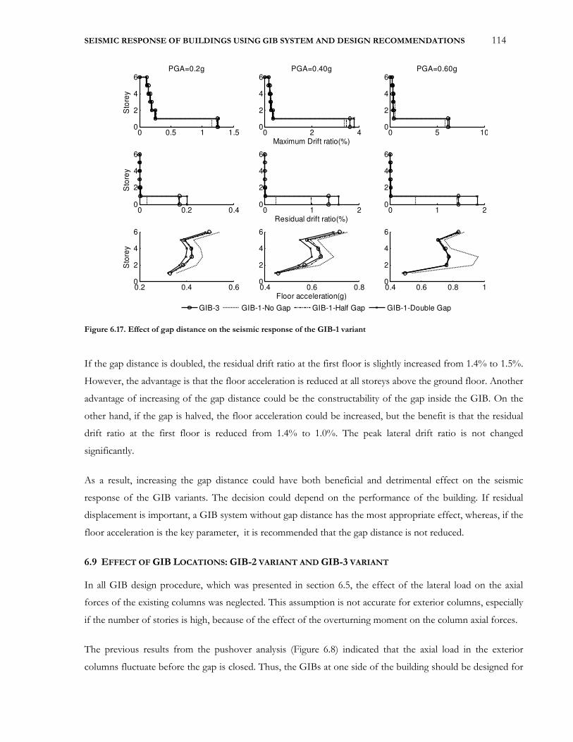
SEISMIC RESPONSE OF BUILDINGS USING GIB SYSTEM AND DESIGN RECOMMENDATIONS 114
Figure 6.17. Effect of gap distance on the seismic response of the GIB-1 variant
If the gap distance is doubled, the residual drift ratio at the first floor is slightly increased from 1.4% to 1.5%.
However, the advantage is that the floor acceleration is reduced at all storeys above the ground floor. Another
advantage of increasing of the gap distance could be the constructability of the gap inside the GIB. On the
other hand, if the gap is halved, the floor acceleration could be increased, but the benefit is that the residual
drift ratio at the first floor is reduced from 1.4% to 1.0%. The peak lateral drift ratio is not changed
significantly.
As a result, increasing the gap distance could have both beneficial and detrimental effect on the seismic
response of the GIB variants. The decision could depend on the performance of the building. If residual
displacement is important, a GIB system without gap distance has the most appropriate effect, whereas, if the
floor acceleration is the key parameter, it is recommended that the gap distance is not reduced.
6.9 EFFECT OF GIB LOCATIONS: GIB-2 VARIANT AND GIB-3 VARIANT
In all GIB design procedure, which was presented in section 6.5, the effect of the lateral load on the axial
forces of the existing columns was neglected. This assumption is not accurate for exterior columns, especially
if the number of stories is high, because of the effect of the overturning moment on the column axial forces.
The previous results from the pushover analysis (Figure 6.8) indicated that the axial load in the exterior
columns fluctuate before the gap is closed. Thus, the GIBs at one side of the building should be designed for
0 0.5 1 1.50
2
4
6PGA=0.2g
Sto
rey
0 0.2 0.40
2
4
6
Sto
rey
0.2 0.4 0.60
2
4
6
Sto
rey
0 2 40
2
4
6PGA=0.40g
Maximum Drift ratio(%)
0 1 20
2
4
6
Residual drift ratio(%)
0.4 0.6 0.80
2
4
6
Floor acceleration(g)
0 5 100
2
4
6PGA=0.60g
0 1 20
2
4
6
0.4 0.6 0.8 10
2
4
6
GIB-3 GIB-1-No Gap GIB-1-Half Gap GIB-1-Double Gap

SEISMIC RESPONSE OF BUILDINGS USING GIB SYSTEM AND DESIGN RECOMMENDATIONS 115
greater forces, than the opposite. This is the second design scenario that is shown in Figure 6.18.b, i.e. GIB-2
variant The design parameters are shown in Table 6.3.b. For GIB-1L and GIB-4R, the design axial load are
increased 55%, while for GIB-1R and GIB-4L, the design axial load is decreased almost 60% and are very low
(almost zero). As a result, these GIBs could be eliminated to reduce the cost of the retrofit as their effects is
negligible. Similarly, the design axial load on GIB-2L and GIB-3R are increased 20%, and the design axial
load on GIB-2R and GIB-2L is decreased 20%.
Figure 6.18. Locations of GIBs
The third scenario (GIB-3) is that the GIB-2R and GIB-3L are eliminated, which is shown in Figure 6.18.c.
Due to the overturning moment only, the axial load on column II and III at the first floor (in one direction)
are decreased 20%. However, this reduction could not be adequate to increase the deformation capacity of
these columns. As a result, this option could not improve the seismic behaviour of soft storey buildings
significantly, but might be beneficial as it reduces the retrofit cost and increases the architectural functionality.
One solution could be to decrease the lateral displacement demand at the first floor (e.g. increasing GIB
angles). This strategy, however, could increase the seismic demand at the storeys upper the first floor.
C-I C-II C-III C-IV
GIB
-3L G
IB-3
R
GIB
-2L
GIB
-2R
GIB
-1L
GIB
-1R
GIB
-4L
GIB
-4R
GIB
-3L G
IB-3
R
GIB
-2L
GIB
-2R
GIB
-1L
GIB
-4R
C-I C-II C-III C-IV
GIB
-3R
GIB
-2L
GIB
-1L
GIB
-4R
C-I C-II C-III C-IV
Table 6.3. GIB configurations for different scenarios
(a-GIB-1)
Column Type
∆GIB ∆Gap Kb
mm mm kN/m
GIB-1L 269 3.65 43315
GIB-1R 269 3.65 43315
GIB-2L 266 3.33 78180
GIB-2R 266 3.33 78180
(b-GIB-2)
Column Type
∆GIB ∆Gap Kb
mm mm kN/m
GIB-1L 225 2.98 92675
GIB-1R - - -
GIB-2L 250 3.00 106170
GIB-2R 292 3.60 49696
(c-GIB-3)
Column Type
∆GIB ∆Gap Kb
mm mm kN/m
GIB-1L 225 2.98 92675
GIB-1R - - -
GIB-2L 250 3.00 106170
GIB-2R - - -

SEISMIC RESPONSE OF BUILDINGS USING GIB SYSTEM AND DESIGN RECOMMENDATIONS 116
Alternatively, the deformation capacity of these columns could be improved using confinement. To achieve
this goal, a GIB- column connection detail is proposed in Chapter 8.
6.9.1 Seismic performance of GIB scenarios
Figure 6.19 shows two demand parameters obtained from incremental dynamic analyses. Overall, all the GIB
variants (dotted lines indicated by circle, square and star for GIB-1, GIB-2 and GIB-3, respectively) have
almost a similar effect on the lateral drift ratio of the soft storey building (Figure 6.19.b). Thus, eliminating four
GIBs from the first floor does not have a significant effect on the seismic demand parameters. However, as it
was mentioned before, one would expect that the drift capacity of GIB-3 variant is not improved
significantly, which is explained in the next paragraph.
Figure 6.19.a shows the ratio of the maximum curvature demand to the ultimate curvature capacity
(deformation damage index DDI) of all beams and columns in all GIB variants. Because all these variants
have soft storey configuration, the maximum DDIs occur at columns of the first floor. DDI of both GIB-I
and GIB-2 variants are very close to each other. Because their displacement demands are almost the same
over the whole range of the intensity level (Figure 6.19.b), the drift capacity of these two variants are also
close to each other. However, the DDI of GIB-2 variant is slightly less than that of GIB-1, which indicates a
potential advantage of the eliminating GIBs at the interior face of exterior columns.
Figure 6.19. Seismic parameters for different GIB scenarios a) DDI, b) Peak floor acceleration
On the other hand, the seismic behaviour of the GIB-3 variant is less improved; its DDI is more than the
other two variants over the whole intensity levels, and the difference increases as the intensity increases. At
the intensity level more than 0.4g, DDI of columns II and III exceeds unity, which indicates that these
columns reach their ultimate capacity. For GIB-1 and GIB-2 variants, this value occurs at the intensity level
almost 0.55g.
0.050.10.150.20.250.30.350.4 0.60
2
4
6
8
Pe
ak in
ters
tore
y d
rift (
%)
PGA(g)
0.050.10.150.20.250.30.350.4 0.60
0.5
1
1.5
2
Pe
ak D
DI
PGA(g)
GIB-1 GIB-2 GIB-3

SEISMIC RESPONSE OF BUILDINGS USING GIB SYSTEM AND DESIGN RECOMMENDATIONS 117
6.10 COLLAPSE POTENTIAL OF CASE STUDY VARIANTS
In order to perform a meaningful assessment of the seismic performance of different scenarios, this section
explores the effect of retrofit scenarios on the reducing the potential of collapse of the soft storey variant. As
such, collapse fragility functions associated to each variant is determined and compared to each other.
To develop collapse fragility curves, the methodology described in ATC-58 [ATC 2007b] was used. As such,
results from the incremental dynamic analysis was used. The intensity at which 50% of the analyses predict
collapse is taken as the median collapse intensity. Using the median value and the dispersion due to record-to-
record variability, the collapse fragility functions are obtained following a lognormal distribution. In this
methodology, collapse is defined as either: sidesway failure, characterized by loss of lateral stiffness and
development of P-Delta instability, or Loss of vertical load carrying capacity of gravity framing members due
to earthquake-induced building drifts.
Figure 6.20 compares the collapse fragility curves for the four variants soft storey SS, full infill FI, GIB-2 and
GIB-3. For a wide range of intensity levels, the probability of collapse of the FI variant is less than the SS
variant. However, when the soft storey is retrofitted using GIB-2 configuration, this probability is reduced
significantly.
Figure 6.20. Collapse fragility curves for different variants
It should be noted that a large number of ground motions (order of 20 records) have been recommended to
obtain reliable estimates of the collapse fragility [ATC 2007b]. Since only 10 ground motions were used in
IDA analyses, these results could be arguable. However, for the purpose of comparison (not absolute
values), it is expected that these results could be acceptable.
6.11 SUMMARY AND CONCLUSION
The case study soft storey frame that were studied in Chapter 3 was retrofitted using the GIB system and
different scenarios of GIB location. It was found that the GIBs that are inside the face of the exterior
columns would not have significant effect on improving the response of the first floor of soft storey
0 0.2 0.4 0.6 0.8 10
0.5
1
Pro
ba
bili
ty o
f co
llap
se
PGA(g)
FI
SS
GIB-1
GIB-3

SEISMIC RESPONSE OF BUILDINGS USING GIB SYSTEM AND DESIGN RECOMMENDATIONS 118
buildings. As a results, these GIBs could be eliminated, which in addition to improve the seismic response of
the soft storey buildings are beneficial due to the architectural and economical aspects.
The last scenario studied was to explore the response of the GIB building if the GIBs that are inside the face
of the interior columns are eliminated in addition to those of the exterior ones. The architectural and the
economic advantage of this solution could be more than the second scenario; however, this strategy could
reduce the displacement capacity of interior columns, and consequently, could increase the possibility of
collapse of the first floor. As such, the displacement capacity of these columns should be increased using
supplemental retrofitting measures including FRP wrapping or steel jacketing. The next chapter proposes a
connection detail between GIBs and existing columns that achieves this goal. In addition, uncertainties
regarding the performance of the GIB system will be discussed in the next chapter.

119
7.FUTURE STUDIES REGARDING THE UNCERTAINTIES OF THE
GIB SYSTEM
7.1 INTRODUCTION
The results of Chapter 5 and Chapter 6 indicated that the presence of the GIB system improves the response
of soft storey buildings significantly. Although, the static and the dynamic behaviour of the GIB system is
obtained based on the theoretical solutions and numerical analyses only, it is expected that its real response
could be similar to the predication. However, a number of questions could be still raised because the GIB
system (or systems with behaviour similar to this) has not been constructed in practice or tested in structural
laboratories. In this chapter, uncertainties regarding the performance of GIB system on the soft storey
response is studied, and future studies to further develop this concept is recommended.
7.2 CONSTRUCTABILITY
One of the major limitations is the constructability of the GIB due to the small distance between the column
and the GIB. For the case study example that was presented in Chapter 5, the offset distance was 50 mm
from the face of the column. Such small offsets could make the brace installation very difficult, or impossible.
Although one solution would be to select a larger distance between the column and the GIB, this would
result in an additional lateral resistance to the system. To deal with this issue, a nonlinear elastic behaviour
could be prescribed for the inclined brace itself. This could be achieved using post tensioning of the inclined
brace, SCED brace [Christopoulos et al. 2008] or using a nonlinear elastic material (such as rubber) in
combination with the inclined brace.
The detailed properties and the related design procedure of such GIB system are not explained here. The
axial-deformation relationship of the inclined brace was obtained from an iteration procedure, and the
relationship was introduced to the numerical modelling. It is, however, recommended that the design
procedure and governing equations of nonlinear GIB be obtained to further develop the proposed system.
The nonlinear elastic behaviour of the inclined brace was modelled using a Ramberg Osgood curve in
SeismoStruct. It was observed that if a nonlinear elastic behaviour is considered for the inclined brace, the
distance between the column and the GIB could be increased to 320 mm. The dotted line in Figure 7.1shows
the hysteretic response of the total system using nonlinear elastic inclined brace, which is close to what is
provided with the linear elastic brace.
Another scenario was studied in which the inclined brace is allowed to yield. This option can be implemented
by using elements such as buckling resistance braces [Sabellia et al. 2003]. The Ramberg Osgood curve with
inelastic behaviour is again defined based on an iteration procedure. In this case, a similar response is
achieved if GIB∆ is adopted as 270 mm, as shown in Figure 7.1 by a dashed line. Although the lateral resistance
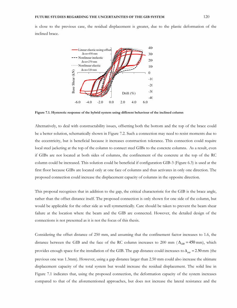
FUTURE STUDIES REGARDING THE UNCERTAINTIES OF THE GIB SYSTEM 120
is close to the previous case, the residual displacement is greater, due to the plastic deformation of the
inclined brace.
Figure 7.1. Hysteretic response of the hybrid system using different behaviour of the inclined column
Alternatively, to deal with constructability issues, offsetting both the bottom and the top of the brace could
be a better solution, schematically shown in Figure 7.2. Such a connection may need to resist moments due to
the eccentricity, but is beneficial because it increases construction tolerance. This connection could require
local steel jacketing at the top of the column to connect steel GIBs to the concrete columns. As a result, even
if GIBs are not located at both sides of columns, the confinement of the concrete at the top of the RC
column could be increased. This solution could be beneficial if configuration GIB-3 (Figure 6.3) is used at the
first floor because GIBs are located only at one face of columns and thus activates in only one direction. The
proposed connection could increase the displacement capacity of columns in the opposite direction.
This proposal recognizes that in addition to the gap, the critical characteristic for the GIB is the brace angle,
rather than the offset distance itself. The proposed connection is only shown for one side of the column, but
would be applicable for the other side as well symmetrically. Care should be taken to prevent the beam shear
failure at the location where the beam and the GIB are connected. However, the detailed design of the
connections is not presented as it is not the focus of this thesis.
Considering the offset distance of 250 mm, and assuming that the confinement factor increases to 1.6, the
distance between the GIB and the face of the RC column increases to 200 mm ( 450GIB∆ = mm), which
provides enough space for the installation of the GIB. The gap distance could increases to 2.50gap
∆ = mm (the
previous one was 1.3mm). However, using a gap distance larger than 2.50 mm could also increase the ultimate
displacement capacity of the total system but would increase the residual displacement. The solid line in
Figure 7.1 indicates that, using the proposed connection, the deformation capacity of the system increases
compared to that of the aforementioned approaches, but does not increase the lateral resistance and the
-400
-300
-200
-100
0
100
200
300
400
-6.0 -4.0 -2.0 0.0 2.0 4.0 6.0
Bas
e S
hea
r (k
N)
Drift (%)
Linear elastic using offset
Nonlinear inelastic
Nonlinear elastic
∆GIB=450 mm
∆GIB=270 mm
∆GIB=320 mm
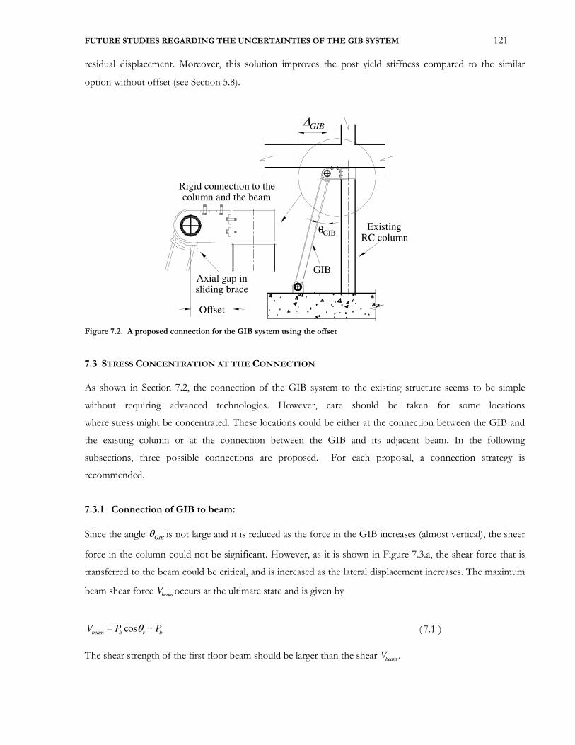
FUTURE STUDIES REGARDING THE UNCERTAINTIES OF THE GIB SYSTEM 121
residual displacement. Moreover, this solution improves the post yield stiffness compared to the similar
option without offset (see Section 5.8).
Figure 7.2. A proposed connection for the GIB system using the offset
7.3 STRESS CONCENTRATION AT THE CONNECTION
As shown in Section 7.2, the connection of the GIB system to the existing structure seems to be simple
without requiring advanced technologies. However, care should be taken for some locations
where stress might be concentrated. These locations could be either at the connection between the GIB and
the existing column or at the connection between the GIB and its adjacent beam. In the following
subsections, three possible connections are proposed. For each proposal, a connection strategy is
recommended.
7.3.1 Connection of GIB to beam:
Since the angle GIBθ is not large and it is reduced as the force in the GIB increases (almost vertical), the sheer
force in the column could not be significant. However, as it is shown in Figure 7.3.a, the shear force that is
transferred to the beam could be critical, and is increased as the lateral displacement increases. The maximum
beam shear force beamV occurs at the ultimate state and is given by
cos beam b r bV P Pθ= � ( 7.1 )
The shear strength of the first floor beam should be larger than the shear beamV .
Existing RC column
∆ GIB
θGIB
Offset
Axial gap in sliding brace
Rigid connection to thecolumn and the beam
GIB

FUTURE STUDIES REGARDING THE UNCERTAINTIES OF THE GIB SYSTEM 122
(a) (b)
Figure 7.3. a)Possibility of Shear failure at the beam and the GIB connection, b) possible retrofit strategy
For configuration GIB-1, the maximum shear force in beams at the first floor obtained from the time history
analysis at the intensity level 0.6g and 0.4g is shown in Table 7.1. The shear force in the exterior face of side
beams, (Corresponding to GIB-1R and GIB-4L) in less than the shear capacity at all intensity levels.
However, at their interior sides (corresponding to GIB-2L and GIB-3R), the shear force exceeds the shear
capacity of beams at both intensity levels. For the middle beam, the shear force exceeds only at the intensity
level 0.6g.
As such, the shear strength of the beam at the location shown in Figure 7.3.b should be increased using
retrofit approaches, such as jacketing, or increase the section area of the beam. However, strengthening of
existing RC beams could not be easy and could require significant effort, which might not be cost effective.
Table 7.1. Shear force in beams at the first floor of the GIB-1 building
Beam properties PGA=0.4g PGA=0.6g
Name type face Shear
Strength(kN)
Shear
Force (KN) Check
Shear
Force(kN) Check
B-S-L Side left 220 130 ok 210 ok
B-S-R Side right 220 290 Not ok 380 Not ok
B-M Middle both 220 210 Not ok 320 Not ok
7.3.2 Connection of GIB to column
Another solution could be that the GIB is connected to the column without any connection to the beam. In
this case, the gusset plate should be located with an offset to the face of the beam, as shown in Figure 7.4.a.
In such case, the axial force in the GIB should be transferred by the gusset plate and the bolts. Thus, these
two components should be designed for the required actions.
Pbsinθr
θr
Pbcosθr
P b
Vbeam =Pb cosθr
Beam Beam
Shear in beam
Vbeam
Vcolumn
Increase the shear
strength of the beam
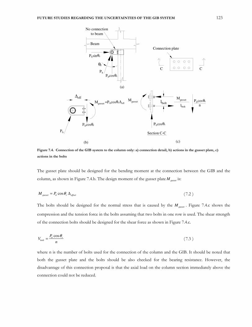
FUTURE STUDIES REGARDING THE UNCERTAINTIES OF THE GIB SYSTEM 123
Figure 7.4. Connection of the GIB system to the column only: a) connection detail, b) actions in the gusset plate, c)
actions in the bolts
The gusset plate should be designed for the bending moment at the connection between the GIB and the
column, as shown in Figure 7.4.b. The design moment of the gusset plate gussetM is:
cos gusset b r offset
M P θ= ∆ ( 7.2 )
The bolts should be designed for the normal stress that is caused by the gussetM . Figure 7.4.c shows the
compression and the tension force in the bolts assuming that two bolts in one row is used. The shear strength
of the connection bolts should be designed for the shear force as shown in Figure 7.4.c.
cos b r
bolt
PV
n
θ= ( 7.3 )
where n is the number of bolts used for the connection of the column and the GIB. It should be noted that
both the gusset plate and the bolts should be also checked for the bearing resistance. However, the
disadvantage of this connection proposal is that the axial load on the column section immediately above the
connection could not be reduced.
Pbsin θr
Beam
θr
Pbcosθr
Pb
No connection
to beam
Pbcosθr
n
Pbcosθr
Mgusset
M gusset
lbolt
lbolt
Section C-CPb
∆off
Mgusset =Pbcosθr ∆off
Pbcosθr
C C
Connection plate
(a)
(b) (c)

FUTURE STUDIES REGARDING THE UNCERTAINTIES OF THE GIB SYSTEM 124
7.3.3 Improved Connection of GIB to column
To improve the disadvantage regarding the previous connection, one possibility could be to strengthen the
flexural capacity of the column at the connection by considering the plate and bolts in the beam like a gusset
flange at the end of the column, as shown in Figure 7.5. Using this connection, the column could be
retrofitted to form a plastic hinge immediately below the connection location, instead of just below the beam
face. The advantage of this proposal is that that the column axial load is reduced at the critical section.
However, the disadvantage is that the confinement of the critical column section would not be increased.
Another alternative might be to transfer the axial forces to the base of column at second floor by cutting
through floor and connecting to the corners. However, this solution could not be cost effective depending on
flooring system.
As a summary, with some additional reflection to the all connection proposed in this section, one might be
able to identify a practical connection detail. An efficient and cost-effective connection strategy is
recommended to be explored as a part of the future development to the GIB system.
Figure 7.5. Alternative connection proposal of GIB to column using gusset plate
7.4 EFFECT OF SUPPLEMENTAL DAMPING ON RESPONSE OF GIB-3 VARIANT
A parametric study was carried out to explore the effect of added dampers on the response of the GIB-3
variant system that were studied in Chapter 6. Since the purpose of this section is to see the effect of the
adding damping on the seismic response of soft storey buildings, the added damper was modelled using a
B B
HSS
ABeam
Gusset
plate
Connection
plateRC
Column
D
D
Section D-D
HSS
Slotted end connection to HSS
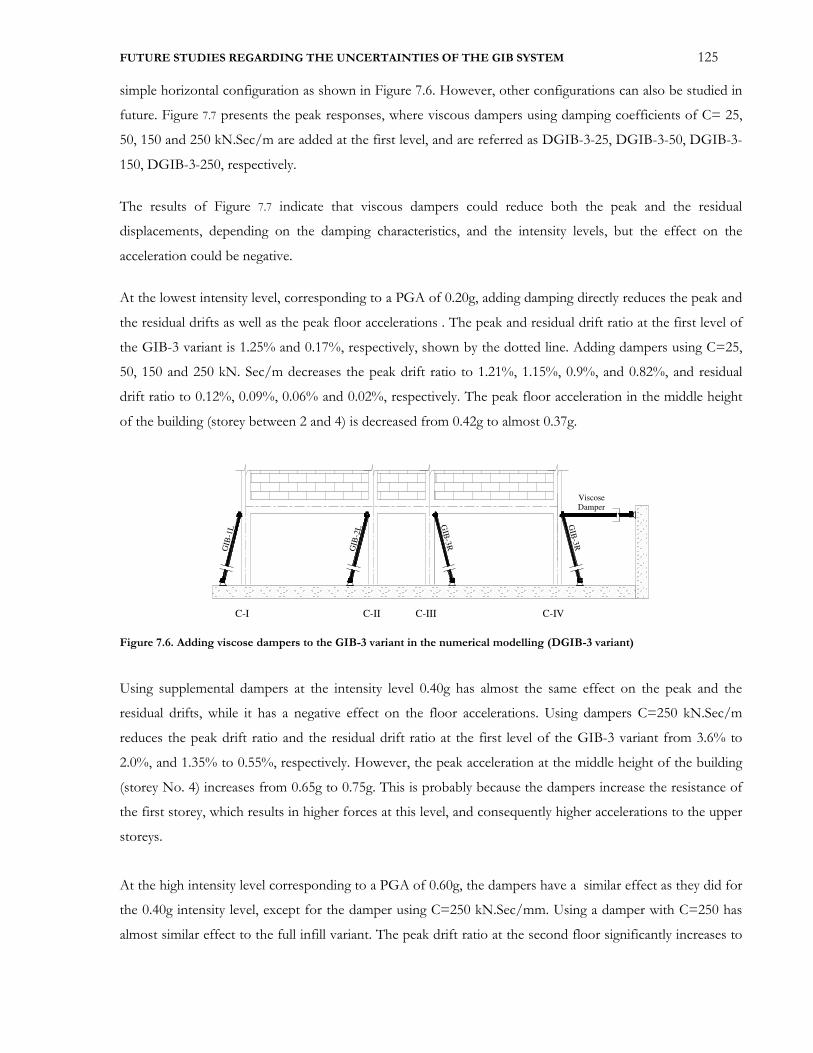
FUTURE STUDIES REGARDING THE UNCERTAINTIES OF THE GIB SYSTEM 125
simple horizontal configuration as shown in Figure 7.6. However, other configurations can also be studied in
future. Figure 7.7 presents the peak responses, where viscous dampers using damping coefficients of C= 25,
50, 150 and 250 kN.Sec/m are added at the first level, and are referred as DGIB-3-25, DGIB-3-50, DGIB-3-
150, DGIB-3-250, respectively.
The results of Figure 7.7 indicate that viscous dampers could reduce both the peak and the residual
displacements, depending on the damping characteristics, and the intensity levels, but the effect on the
acceleration could be negative.
At the lowest intensity level, corresponding to a PGA of 0.20g, adding damping directly reduces the peak and
the residual drifts as well as the peak floor accelerations . The peak and residual drift ratio at the first level of
the GIB-3 variant is 1.25% and 0.17%, respectively, shown by the dotted line. Adding dampers using C=25,
50, 150 and 250 kN. Sec/m decreases the peak drift ratio to 1.21%, 1.15%, 0.9%, and 0.82%, and residual
drift ratio to 0.12%, 0.09%, 0.06% and 0.02%, respectively. The peak floor acceleration in the middle height
of the building (storey between 2 and 4) is decreased from 0.42g to almost 0.37g.
GIB
-3R
GIB
-2L
GIB
-1L
C-I C-II C-III C-IV
GIB
-3R
ViscoseDamper
Figure 7.6. Adding viscose dampers to the GIB-3 variant in the numerical modelling (DGIB-3 variant)
Using supplemental dampers at the intensity level 0.40g has almost the same effect on the peak and the
residual drifts, while it has a negative effect on the floor accelerations. Using dampers C=250 kN.Sec/m
reduces the peak drift ratio and the residual drift ratio at the first level of the GIB-3 variant from 3.6% to
2.0%, and 1.35% to 0.55%, respectively. However, the peak acceleration at the middle height of the building
(storey No. 4) increases from 0.65g to 0.75g. This is probably because the dampers increase the resistance of
the first storey, which results in higher forces at this level, and consequently higher accelerations to the upper
storeys.
At the high intensity level corresponding to a PGA of 0.60g, the dampers have a similar effect as they did for
the 0.40g intensity level, except for the damper using C=250 kN.Sec/mm. Using a damper with C=250 has
almost similar effect to the full infill variant. The peak drift ratio at the second floor significantly increases to
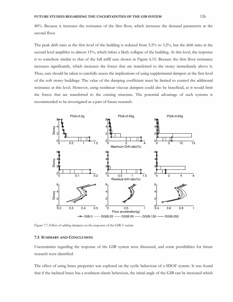
FUTURE STUDIES REGARDING THE UNCERTAINTIES OF THE GIB SYSTEM 126
40%. Because it increases the resistance of the first floor, which increases the demand parameters at the
second floor.
The peak drift ratio at the first level of the building is reduced from 5.5% to 3.2%, but the drift ratio at the
second level amplifies to almost 15%, which infers a likely collapse of the building. At this level, the response
is to somehow similar to that of the full infill case shown in Figure 6.15. Because the first floor resistance
increases significantly, which increases the forces that are transferred to the storey immediately above it.
Thus, care should be taken to carefully assess the implications of using supplemental dampers at the first level
of the soft storey buildings. The value of the damping coefficient must be limited to control the additional
resistance at this level. However, using nonlinear viscous dampers could also be beneficial, as it would limit
the forces that are transferred to the existing structure. The potential advantage of such systems is
recommended to be investigated as a part of future research.
Figure 7.7. Effect of adding dampers on the response of the GIB-3 variant
7.5 SUMMARY AND CONCLUSION
Uncertainties regarding the response of the GIB system were discussed, and some possibilities for future
research were identified.
The effect of using brace properties was explored on the cyclic behaviour of a SDOF system. It was found
that if the inclined brace has a nonlinear elastic behaviour, the initial angle of the GIB can be increased which
0 0.5 1 1.50
2
4
6PGA=0.2g
Sto
rey
0 0.1 0.20
2
4
6
Sto
rey
0.2 0.3 0.4 0.50
2
4
6
Sto
rey
0 2 40
2
4
6PGA=0.40g
Maximum Drift ratio(%)
0 0.5 1 1.50
2
4
6
Residual drift ratio(%)
0 0.5 10
2
4
6
Floor acceleration(g)
0 5 10 150
2
4
6PGA=0.60g
0 2 4 60
2
4
6
0.4 0.6 0.8 10
2
4
6
GIB-3 DGIB-25 DGIB-50 DGIB-150 DGIB-250
FUTURE STUDIES REGARDING THE UNCERTAINTIES OF THE GIB SYSTEM 127
could improve the construction of the GIB. The increase in angle, however, did not affect the total response.
Alternatively, it was suggested that both the bottom and the top of the brace are offset. This solution can
increases the construction tolerance of the connection in addition to increase the column confinement.
Some possible types of connections of the GIB system to exiting columns were proposed and illustrated. In
the first proposal, the GIB system is connected to both the beam and the column. The connection requires
that the beam is checked for shear and possible strengthening. The second proposal was that the GIB system
is connected to the column only. In this case, the gusset plate and the connectors should be strong enough to
ensure that the vertical forces are transferred to the GIB system.
The effect of supplemental viscous damping on the seismic response of the soft storey building was
investigated through a parametric study. It was found that adding damping could reduce both the ultimate
and the residual deformations. However, at high intensity levels, dampers could have negative effects on the
response; using viscous damping with high damping coefficient could increase the lateral resistance of the
first floor.
128
8.CONCLUSIONS
Although each chapter outlined related results and conclusions separately, the main conclusion of this work is
to, however, raise the question that has not been asked for a few decades: Can buildings with soft storey
configurations perform well in earthquakes? The real behaviour of such buildings in the past earthquakes
might give a negative answer to this question. However, the results of this thesis provided an insight that
intelligent and efficient soft storey structures could have an acceptable seismic performance. The gapped
inclined brace GIB system was one solution that this work proposed to retrofit soft storey buildings. This
strategy in addition to take their architectural and structural advantages, it mitigated the collapse possibility in
strong ground motions.
The following sections of this chapter provide an overview of the previous chapters and integrate their results
to show how this work has responded to the objectives that were outlined in Chapter 1.
8.1 CHAPTER 1 AND 2
This work began with a brief literature review on the performance of buildings with soft storey
configurations. Their potential advantages of such buildings in the architectural and the structural point of
view were discussed. Various types of buildings with such configurations were categorised in Chapter 2.
Typical problems associated with such buildings and their failure mechanisms in the past earthquakes were
summarised.
Chapter 1 and 2 showed that among the available buildings with soft storey configuration, buildings that
masonry infills are disconnected in the first floor are the most common type. In addition, earthquake surveys
have shown that discontinuous infills in the first floors are very likely to cause a soft-storey mechanism at the
ground level.
8.2 CHAPTER 3
Thus, Chapter 3 started the numerical case study assessment on a six-storey reinforced concrete frame
building for two scenarios of full masonry infill and partial and with soft-storey response developing at the
ground storey for the partial infill case. Incremental nonlinear time history analyses were used to compare the
seismic response of the two scenarios. Potential advantages of each scenario in different hazard level were
discussed.
The incremental non-linear time history analysis results in Chapter 3 illustrated that peak floor accelerations
in partial infill case are less than the full infill case, which can reduce damage to non-structural elements. In
addition, the peak and residual inter storey drift at storeys above the open ground floor was highly reduced.
CONCLUSIONS 129
However, the potential of collapse of the partial infill case was increased as the intensity level is increased,
reflecting the observations made in past earthquakes.
8.3 CHAPTER 4
The effect of some key characteristics including P-Delta effects and post yield stiffness on the behaviour of
soft first storey buildings was explored in Chapter 4. The results of static cyclic analyses of RC columns with
different geometrical and mechanical properties were used to highlight the influence of some characteristics
such as bar ratio, section dimensions, axial load ratio and confinement factor on the lateral resistance and drift
capacity of RC columns. The implications of the analysis findings were discussed in relation to potential
retrofit schemes.
The analysis results on Chapter 4 indicated that if the gravity load system could be de-coupled from the lateral
load resisting system, this could help reduce the likely deformation demands, which tend to be amplified by
P-delta effects. In addition, it was demonstrated that if the axial load on column sections could be reduced,
their deformation capacities could be significantly increased. Thus, a potentially effective and innovative
means of retrofitting a structure with an open-ground storey were proposed by introducing a series of gravity
columns at the ground level that slide with the first storey. By doing this, P-delta effects were minimised, and
the deformation capacity of the first storey columns were increased, without significantly affecting their lateral
strength and potential for energy dissipation.
8.4 CHAPTER 5
The limitation of this proposed retrofitting strategy were discussed in the beginning of Chapter 5, and then
gapped inclined brace GIB system were alternatively proposed that could reduce the drawbacks of the sliding
gravity columns proposal, while takes the positive aspects. The mechanics of the proposed system was
illustrated, and a brace sizing procedure was proposed.
The results from pushover analyses of RC columns with different configurations verified various
mathematical relations developed for the purpose of sizing the braces. It was concluded that increasing
confinement in addition to the proposed approach could also improve the deformation capacity of RC
columns. Nonlinear quasi-static cyclic analysis of a single span RC frame indicated that the proposed strategy
could significantly improve the hysteretic response of a soft storey frame in terms of energy dissipation
capacity and residual deformation.
8.5 CHAPTER 6
The dynamic characteristics of MDOF buildings that were retrofitted using the GIB system at the ground
floor were investigated in Chapter 6. Design considerations based incorporating the soft storey mechanisms

CONCLUSIONS 130
were briefly presented in this chapter. Subsequently, the buildings that were studied in chapter 3 retrofitted
using the GIB system, and the numerical results were compared using different scenarios of GIB locations.
The numerical analysis of the retrofitted soft storey building indicated that the GIBs that are inside the
exterior columns don't have significant effect of the improving the response. As results, these GIBs could be
eliminated at the ground floor of soft storey buildings, which are beneficial due to the architectural and
economical aspects.
8.6 CHAPTER 7
Chapter 7 discussed uncertainties regarding the response of the GIB system and described recommend issues
to be investigated in future research. Some aspects including construction issues and connection
considerations were briefly discussed. The effect of supplemental vicious damping in addition to the GIB
system was initially investigated to further develop the concept as a part of future studies.
This chapter concluded that if the inclined brace has a nonlinear elastic behaviour, the initial angle of the GIB
can be increased which could improve the construction of the GIB. Alternatively, it was suggested that both
the bottom and the top of the brace are offset to increase the construction tolerance in addition to increase
the column confinement.
It was also found that adding damping could reduce both the ultimate and the residual deformations.
However, at high intensity levels, dampers could have negative effects on the response, because their effect of
the lateral resistance is higher than reducing accelerations.
It is, however, recommended that dynamic analyses of more case studies be carried out along with
experimental validations to further develop the proposed system and demonstrate its applicability for the
seismic upgrade of soft storey structures.

131
REFERENCES
Adam, C., Jager, C. [2011] “Seismic Induced Global Collapse of Non-deteriorating Frame Structures,”
Computational Methods in Earthquake Engineering, Computational Methods in Applied Sciences, Vol. 99, pp.
21-40.
Arnold, C. [1984] “Soft first stories: truths and myths,” Proc. 8th WCEE, San Francisco, California.
ATC-52-3 [2009] “Here Today—Here Tomorrow,The Road to Earthquake Resilience in San Francisco,
Earthquake Safety for Soft-Story Buildings,” Redwood City,.
Benjamin, J.R., Cornell, C.A. [1970] Probability, statistics, and decision for civil engineers, Hill Book Company- 684 p,
New York, McGraw.
Bernal, D. [1987] “Amplification factors for inelastic dynamic P-∆ effects in earthquake analysis,” Earthquake
Engineering and Structural Dynamics, Vol. 15, No. 5, pp. 635–651.
Bernal, D. [1998] “Instability of buildings during seismic response ” Engineering Structures, Vol. 20, pp. 496-
502.
Bertero, V.V. [1984] “SEISMIC BEHAVIOR OF R/C WALL STRUCTW SYST,” Journal of Structural
Engineering, Vol. 110, No. 8, pp. 1803-1821.
Bertero, V.V. [1997] “illustrated introduction to earthquake engineering principles,” Berkeley.
Bertoldi, S.H., Decanini, L.D. and Gavarini, [1993] “Telai tamponati soggetti ad azione sismica, un modello
semplificato: confronto sperimentale e numerico,” ANIDIS, Vol. 2, pp. 815-824,.
Bilham, R. [2004] “Urban Earthquake Fatalities: A Safer World, or Worse to Come?,” Research Letters, Vol. 75,
No. 6, pp. 706-712.
Blakeborough, A. [1994] “The Northridge California Earthquake of 17 Jan 1994,” London.
Boardman, P.R., Wood, B.J., Carr, A.J. [1983] “Union House - A cross braced structure with energy
dissipators.,” Bulletin of the New Zealand Society for Earthquake Engineering, Vol. 16, No. 2, pp. 83-97.
Bommer, J.J., Martinez-Pereira, A. [1999] “The effective duration of earthquake strong motion,” Journal of
Earthquake Engineering & Structural Dynamics, Vol. 3, pp. 127-172.
Bonowitz, D. [2005] “Earthquake risk in residential buildings,” from
http://www.ci.berkeley.ca.us/contentdisplay.aspx?id=622.
Carr, A.J. [2004] “Ruaumoko Program for Inelastic Dynamic Analysis – Users Manual,” Christchurch ,New
Zealand.
Ceballos, C., Sullivan, T.J. [2011] “Development of Improved Inelastic Displacement Prediction Equations
for the Seismic Design of Hybrid Systems,” Bulletin of the New Zealand Society for Earthquake Engineering,
Vol. 44, No. 3, pp. 167.
CEN [2004] “Eurocode 8: Design of structures for earthquake resistance -Part 1: General rules, seismic
actions and rules for buildings,” Brussels, Belgium.
REFERENCES 132
Chen, Y.Q., Constantinou, M.C. [1990] “ Use of Teflon sliders in a modification of the concept of soft first
storey,” Engineering Structures, New Zealand, Vol. 12, No. 4, pp. 243-252.
Chopra, A.K., Clough, D.P., Clough, R.W. [1973] “Earthquake resistance of buildings with a soft first story,”
Earthquake Engineering& Structural. Dynamics, Vol. 1, No. 4, pp. 347-355.
Christopoulos, C., Pampanin, S., Priestley, M.J.N. [2003] “Performance-based seismic response of frame
structures including residual deformations. Part 2: Multi-degree of freedom systems,” Journal of
Earthquake Engineering, Vol. 7, No. 1, pp. 119-147.
Christopoulos, C., Tremblay, R., Kim, H.J., Lacerte, M. [2008] “Self-centering energy dissipative bracing
system for the seismic resistance of structures: Development and validation,” Journal of Structural
Engineering-Asce, Vol. 134, No. 1, pp. 96-107.
Colangelo, F. [1999] “Qualificazione, risposta sismica pseudodinamica e modelli fenomenologici di portali,”
(in Italian) DISAT.
Comerio, M.C. [1995] “Northridge housing losses, a study for the California Governor’s Office of
Emergency Services,” University of California, Berkeley.
Crisafulli, F.J. [1997] “Seismic Behaviour of Reinforced Concrete Structures with Masonry Infills.”
Daniell, J.E., Khazai, B., Wenzel, F., Vervaeck, A. [2011] “The CATDAT damaging earthquakes database,”
Natural Hazards and Earth System Sciences, Vol. 11, No. 8, pp. 2235-2251.
Deierlein, G.G., Reinhorn, A.M., Willford, M.R. [2010] “Nonlinear Structural Analysis For Seismic Design -
A Guide for Practicing Engineers,” 4, U.S. department of Commerce.
EFFIT [1993] “The Loma Prieta Earthquaje of 17 October 1989,” London.
Elwood, K. [2002] “Shake table tests and analytical studies on the gravity load collapse of reinforced concrete
frames,” Ph.D, University of California, Berkeley.
Emori, K., Schonbrich, W.C. [1978] “Analysis of reinforced concrete framewall structures for strong
motion earthquakes,” University of Illinois, Urbana, Illinois, USA.
Esteva, L. [1992] “Nonlinear Seismic Response of Soft-First-Storey Buildings Subjected to Narrow Band
Accelerograms,” Earthquake Spectra, Vol. 8, No. 3, pp. 373-389.
Fardis, M.N., Biskinis, D.E. [2003] “Deformation capacity of RC members, as controlled by flexure or shear,”
In Performance based Engineering for Earthquake Resistant Reinforced Concrete Structures: A Volume Honoring
Shunsuke Otani, University of Tokyo.
Fierro, E., Perry, C. [2010] “Preliminary Reconnaissance Report -12 January 2010 Haiti Earthquake ” from
http://peer.berkeley.edu/publications/haiti_2010/documents/Haiti_Reconnaissance.pdf.
Filler, M. [2009] “Le Corbusier: The Art of Architecture an exhibition at the Barbican Art Gallery, London,
February 19-May 24, 2009,” New York Review of Books, Vol. 56, No. 7, pp. 33-36.
Fintel, M., Khan, F.R. [1969] “Shock-absorbing soft storey concept for multistorey earthquake structures,”
ACI J., Vol. 66, pp. 381-390.
REFERENCES 133
Galli [2006] “EVALUATION OF THE SEISMIC RESPONSE OF EXISTING R.C. frame Building with
masonry infills,” Msc, Rose School, IUSS, Pavia, Italy.
Glassman, P. [2001] “Le Corbusier and the continual revolution in architecture.,” Library Journal, Vol. 126,
No. 2, pp. 85-85.
Green, N.B. [1935] “Flexible first story construction for earthquake resistance,” Transactions, American Society of
Civil Engineers, Vol. 100, No. 1, pp. 645-674.
Guevara-Perez, L.T. [2010] “Seismic Regulations Versus Modern Architectural And Urban Configurations,”
Journal of Disaster Research, Vol. 5, No. 5.
Hak, S., Morandi, P., Magenes, G., Sullivan, T.J. [2012] “Damage Control for Clay Masonry Infills in the
Design of RC Frame Structures,” Journal of Earthquake Engineering, Vol. 16, pp. 1-35.
Hancock, J., Bommer, J.J. [2006] “A state-of-knowledge review of the influence of strong-motion duration on
structural damage,” Earthquake Spectra, Vol. 22, No. 3, pp. 827-845.
Jacobsen, L.S. [1938] “Effects of a flexible first storey in a building located on vibrating ground,” S.
Timoshenko 60th Anniversary Volume, New York.
Jennings, P.C., Husid, R. [1968] “Collapse of yielding structures during earthquakes,” Journal of the Engineering
Mechanics Division Proc. (ASCE), Vol. 94, pp. 1045–1065.
Kawashima Laboratory from www.seismic.cv.titech.ac.jp.
King, D.J., Priestley, M.J.N., Park, R. [1986] “Computer Programs for Concrete Column Design, Res. Report
86/12,” Department of Civil Engineering, University of Canterbury, New Zealand.
Kowalsky, M.J. [2000] “Deformation limit states for circular reinforced concrete bridge columns,” J. Struct.
Eng-ASCE, Vol. 126, No. 8, pp. 869-878.
Lam, S., Wu, B., Wong, Y., Wang, Z., Liu, Z., CS, L. [2003] “Drift capacity of rectangular reinforced concrete
columns with low lateral confinement and high-axial load,” Journal of Structural Engineering (ASCE),
Vol. 129, No. 6, pp. 733–742.
MacQuarrie, J. [2005] “A Hard Look at Soft Stories, Housing in Berkeley,” from
http://www.ci.berkeley.ca.us/contentdisplay.aspx?id=622.
MacRae, G. [1994] “P-∆ effects on single-degree-of-freedom structures in earthquake,” Earthquake Spectra,
Vol. 10, pp. 539–568.
Mahin, S.A., Bertero, V.V., Chopra, A.K., Collins, R.G. [1976a] “Response of the Olive View Hospital Main
Building during the San Fernando Earthquake,” Berkeley, California.
Mahin, S.A., Bertero, V.V., Chopra , A.K., Collins, R.G. [1976b] “Response of the Olive View Hospital main
building during the San Fernando earthquake,” 76-22, Berkeley (USA): .
Maley, T.J., Roldán, R., Lago, A., Sullivan, T.J. [2013] “Effects of response spectrum shape on the response
of steel frame and frame-wall structures,” IUSS Press, R. R. R., Pavia, Italy.
Mander, J.B., Priestley, M.J.N., Park, R. [1988] “Theoretical Stress-Strain Model for Confined Concrete,”
Journal of Structural Engineering-Asce, Vol. 114, No. 8, pp. 1804-1826.
REFERENCES 134
Martel, R.R. [1929] “The effects on earthquakes on buildings with a flexible first story,” Bulletin of the
Seismological Society of America, Vol. 19, No. 3.
Naeim, F.e. [1989] The Seismic Design Handbook, Van Nostrand Reinhold.
Neuenhofer, A., Filippou, F.C. [1997] “Evaluation of nonlinear frame finite-element models,” Journal of
Structural Engineering and Mechanics, Vol. 123, No. 7, pp. 958-966.
NISEE [1972] “Casa Micasa Building,” from http://nisee.berkeley.edu/elibrary/Image/GoddenJ71.
NISEE [1979] “Imperial County Services Building,” from
http://nisee.berkeley.edu/elibrary/Image/GoddenJ76.
NISEE [1999] “Soft strey collapse in Turkey earthquake (Izmit 1999),” from
http://nisee.berkeley.edu/elibrary/search?in=0&ss=izmit+concrete&start=61.
NISEE [2010a] “Olive View Hospital, Sylmar,” from http://nisee.berkeley.edu/elibrary/Image/GoddenJ72.
NISEE [2010b] “Partial collapse of concrete residential building in Port-au-Prince, Haiti,” from
http://nisee.berkeley.edu/elibrary/Image/201005144.
NIST [1997] “The UW-PEER Reinforced Concrete Column Test Database,” from
http://www.ce.washington.edu/~peera1/.
Otani, S. [1974] “A Computer Program for Inelastic Response of R/C Frames to Earthquakes,” Civil
Engineering Studies, Univ. Of Illinois at Urbana-Champaign.
Pampanin, S., Moratti, M., Calvi, G.M. [2002] “Seismic Behaviour of R.C. Beam-Column Joints Designed for
Gravity Loads,” 12th European Conference on Earthquake Engineering, London.
Park, H.S., Paulay, T. [1975] Reinforced Concrete Structures, New York, John Wiley and Sons.
Paulay, T., Priestley, M.J.N. [1992] Seismic Design of Reinforced Concrete and Masonry Buildings, New York.
Pauschke, J.M., Oliveira, C.S., Shah, H.C., Zsutty, T.C. [1981] “A preliminary investigation of the dynamic
response of the Imperial County Services Building during the October 15, 1979 Imperial Valley
earthquake,” 94.
Poling, C.V. [1977] “'Design and Form Basic Course at Bauhaus and Later' - Itten,J,” Art Journal, Vol. 36, No.
4, pp. 368-&.
Priestley, M.J.N., Calvi, G.M., Kowalsky, M.J. [2007] Displacement Based Seismic Design of Structures, IUSS, Pavia,
Italy.
Ruiz-Garcia, J. [2010] “On the influence of strong-ground motion duration on residual displacement
demands,” Earthquakes and Structures, Vol. 1, No. 4, pp. 17.
Rutenberg, A., Jennings, P.C., Housner, G.W. [1982] “The response of veterans hospital building 41 in the
San Fernando earthquake,” Erq. Eng & struct. Dyn, Vol. 10, No. 3.
Sabellia, R., Mahin, S., Changc, C. [2003] “Seismic demands on steel braced frame buildings with buckling-
restrained braces,” Engineering Structures, Vol. 25, pp. 655-666.
Selvaduray, G., Vukazich, S., Arnold, S., Tran, J. [2003] “Inventory of Soft-First Story Multi-Family Dwellings
in Santa Clara County,” San Jose, CA.

REFERENCES 135
Sharma, A., Eligehausenb, R., Reddya, G.R. [2011] “A new model to simulate joint shear behavior of poorly
detailed beam–column connections in RC structures under seismic loads, Part I: Exterior joints,”
Engineering Structures, Vol. 33, No. 3, pp. 1034-1051.
Shome, N. [1999] “Probablistic seismic demand analysis of nonlinear structures,” Ph.D., Department of civil
and environmental engineering, Stanford University, Stanford
Stafford, S. [1969] “A method of analysis for infilled frames,” Proceedings of the institution of civil engineers, Vol. 44,
pp. 31-48.
Sullivan, T.J., Calvi, G.M. [2011] “Consideration for seismic assessment of buildings using the direct
displacement based assessment approach,” ANIDIS, Bari.
Todorovska, M.I. [1999] “Base isolation by a soft first story with inclined columns,” Journal of Engineering
Mechanics, ASCE, Vol. 125, No. 4, pp. 448-457.
Trifunac, M.D., Brady, A.J. [1975] “A study on the duration of strong earthquake ground motion,” B.Seismol.
Soc. Am, Vol. 65, No. 3, pp. 223-241.
Trowland, M. [2003] “Modelling the Shear Hinge in Beam Column Joints,” Univ. of Canterbury Department
of Civil Engineering, New Zealand.
UBC [2009] “United Building Code ”.
USGS [2013] “Earthquakes. Internet resource,,” Retrieved February 20, 2013, from
http://earthquake.usgs.gov/earthquakes/.
Vukazich, S.M., Selvaduray, G., Tran, J. [2006] “Conducting a soft first-story multifamily dwelling survey: An
example using Santa Clara County, California,” Earthquake Spectra, Vol. 22, No. 4, pp. 1063-1079.