reTORT Optical Design Software: Triplet to GRIN Use Case

reTORT Optical Design Software: Triplet to GRIN Use Case

reTORT Optical Design Software:

Triplet to GRIN Use Case

1 Introduction

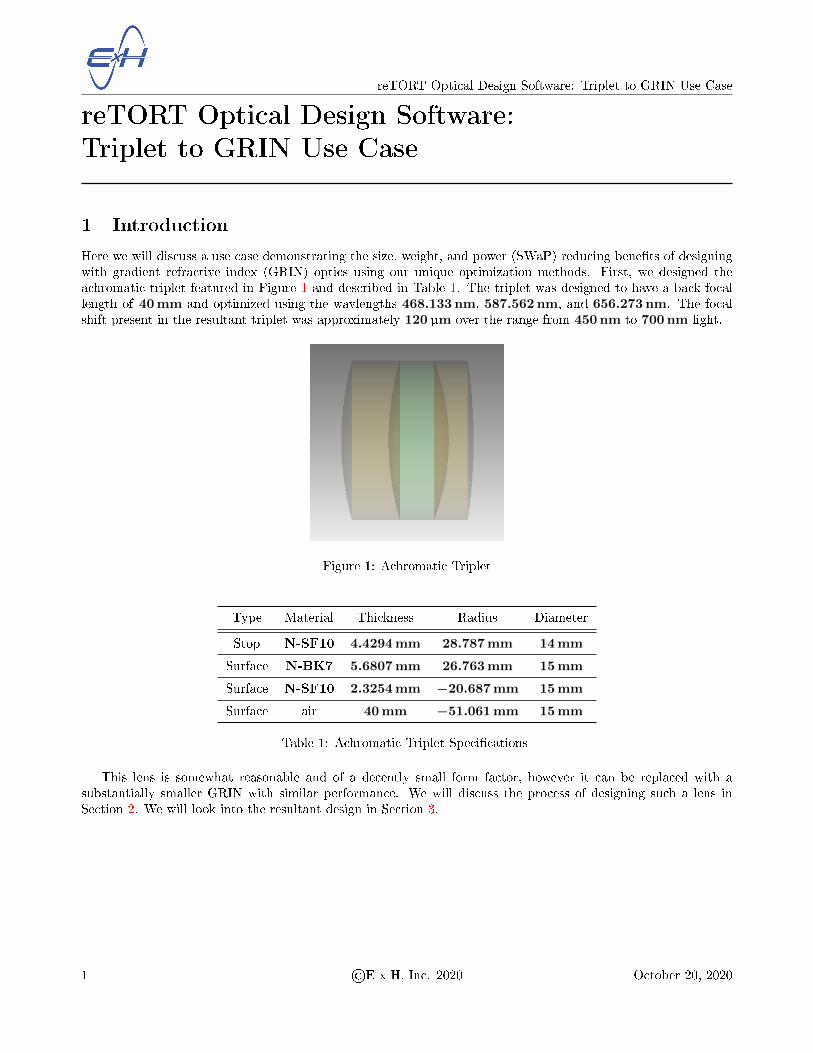
Here we will discuss a use case demonstrating the size, weight, and power (SWaP) reducing bene�ts of designingwith gradient refractive index (GRIN) optics using our unique optimization methods. First, we designed theachromatic triplet featured in Figure 1 and described in Table 1. The triplet was designed to have a back focallength of 40mm and optimized using the wavlengths 468.133 nm, 587.562 nm, and 656.273 nm. The focalshift present in the resultant triplet was approximately 120 µm over the range from 450 nm to 700 nm light.

Figure 1: Achromatic Triplet

Type Material Thickness Radius Diameter

Stop N-SF10 4.4294mm 28.787mm 14mm

Surface N-BK7 5.6807mm 26.763mm 15mm

Surface N-SF10 2.3254mm −20.687mm 15mm

Surface air 40mm −51.061mm 15mm

Table 1: Achromatic Triplet Speci�cations

This lens is somewhat reasonable and of a decently small form factor, however it can be replaced with asubstantially smaller GRIN with similar performance. We will discuss the process of designing such a lens inSection 2. We will look into the resultant design in Section 3.

1 ©E x H, Inc. 2020 October 20, 2020


2 Creating the GRIN

Here we will describe the steps required to appropriately generate a GRIN design using reTORT to replace thetriplet described in Section 1. For this application, we will give reTORT quite a number of variables to workwith and allow it to design the lens for us. The following steps will guide you through the process of setting upthis kind of design.

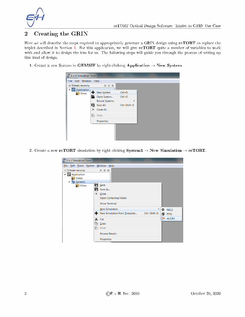
1. Create a new System in GEMSIF by right-clicking Application → New System.

2. Create a new reTORT simulation by right-clicking System1 → New Simulation → reTORT.

2 ©E x H, Inc. 2020 October 20, 2020


3. You will now see the default reTORT system that can be used as a starting point for your optical system.The default source (BeamSource1) uses the set of three wavelengths described in Section 1, however toappropriately design for this lens we will also need ray bundles from multiple incident angles. To change this,expand reTORT under theModel Hierarchy and also expand reTORT→ Sources→ BeamSource1.Click on the BeamSource1 to open its Property Editor.

4. Modify the Incident Elevation Angles �eld to contain 2° in addition to the default 0° (separated bycommas).

5. Next, we need to import materials to build a GRIN lens. We will use a Binary Mixture which allowsus to take two dispersive materials and mix them using a polynomial mixing fraction ranging from 0 to 1where 0 indicates 100% of the �rst material and 1 indicates 100% of the second material. First we willimport the constituent materials. Open the Material Import window by right-clicking on Materials →Import Material from Database. For the �rst material, select Glass→ BK7→ N-BK7 (SCHOTT)and click Import.

6. For the second material, open the Material Import window again and select Glass → SF10 → N-SF10(SCHOTT) and click Import. You should now have two glass materials listed under Materials withinthe Model Hierarchy.

3 ©E x H, Inc. 2020 October 20, 2020


7. Now create a binary mixture by right-clicking on Materials → PolynomialMaterialMixtures → NewCrossPolynomialBinaryMixture. Clicking on your newly created CrossPolynomialBinaryMixtureunderMaterials should display its Property Editor. This editor will allow you to de�ne the two materialsthat compose the binary mixture and also the material mixing fraction coe�cients. Keep in mind that whilethese coe�cients are de�ned according to the polynomial, they do not directly map to the refractive indicesas they directly determine proportion of the two materials at any given point.

8. Change the CrossPolynomialBinaryMixture's properties for Material 1 to BK7 and Material 2 toSF10.

9. Change the following Material Coe�cients to the following values C0 (Base Proportion) → 0.5, C1(r�2) → 0.005, C2 (r�4) → 0.0.

4 ©E x H, Inc. 2020 October 20, 2020


10. The next step will be to build our GRIN singlet lens element. Under Elements in the Model Hierarchy,select LensStack1.

11. In the Property Editor, add a new surface to the lens stack by clicking the Add button. There shouldnow be three surfaces in the lens stack, including the default Stop and Image Plane.

12. Change the Thickness of the �rst surface to 3mm and its Diameter to 14mm. Then set its ClearAperture Margin to 1mm. This will shrink the diameter of the source to match the aperture stop, whilekeeping the incident angles within the bounds of the lens.

13. Change the second surface's Diameter to 15mm. Then set its Thickness to 40mm, to specify theworking distance from the image plane.

14. Change the material of the �rst surface by double-clicking the entry under the Material column andselecting CrossPolynomialBinaryMixture from the dropdown. Leave the default Radius of 0mm forall surfaces, which speci�ces a planar surface.

15. Click on the X/Z plane orientation button on your ModelView window:

Right-click on the reTORT simulation and select Run All. Your ModelView should now show the lensand a ray-trace of both speci�ed angles as in the below image.

5 ©E x H, Inc. 2020 October 20, 2020


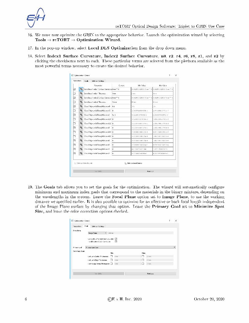
16. We must now optimize the GRIN to the appropriate behavior. Launch the optimization wizard by selectingTools → reTORT → Optimization Wizard.

17. In the pop-up window, select Local DLS Optimization from the drop down menu.

18. Select Index1 Surface Curvature, Index2 Surface Curvature, n0, r2, r4, r6, r8, z1, and z2 byclicking the checkboxes next to each. These particular terms are selected from the plethora available as themost powerful terms necessary to create the desired behavior.

19. The Goals tab allows you to set the goals for the optimization. The wizard will automatically con�gureminimum and maximum index goals that correspond to the materials in the binary mixture, depending onthe wavelengths in the system. Leave the Focal Plane option set to Image Plane, to use the workingdistance we speci�ed earlier. It is also possible to optimize for an e�ective or back focal length independentof the Image Plane surface by changing that option. Leave the Primary Goal set to Minimize SpotSize, and leave the color correction options checked.

6 ©E x H, Inc. 2020 October 20, 2020


20. The �nal pane of the wizard allows con�guration options to be changed for the global and local optimizations.The default values of 100 function evaluations and 100 maximum iterations should �nd a good solution formany systems. Now click Run Local.

21. The optimization should now take a few moments and result with a well focusing GRIN.

Here is a ray-trace of the �nal system:

To show a cleaner ray-trace, click the Choose Ray Bundles button ( ) at the top of the model viewand select Show Ray Planes → Meridonal from the drop-down menu.

The �nal set of parameters might look something like in Table 2 below.

7 ©E x H, Inc. 2020 October 20, 2020


Name Value

C0(n0) 0.730395

C1(r^2) −0.00597105

C2(r^4) −8.37334 · 10−5

C3(r^6) 4.69635 · 10−7

C4(r^8) −2.66420 · 10−8

C6(z^1) 0.0320444

C7(z^2) 0.00818006

Surface 1 Radius 23.1175mm

Surface 2 Radius −77.3678mm

Table 2: Optimized Coe�cients

Now you have generated the actual design of the GRIN. In Section 3 we will brie�y analyze this design. Appendix Adescribes some additional metrics for analyzing the design and how to generate them.

8 ©E x H, Inc. 2020 October 20, 2020


3 Design Conclusion

We can see the size requirements, and subsequently weight requirements, are dramatically reduced with theresultant GRIN vs the original triplet from Section 1, but now we must analyze the performance to verify thatthe design is a reasonable one. For comparison we will look at focal drift plots for each design as shown inFigure 2. For instructions on the creation of these plots, please see Appendix B. As you can see, both designsdemonstrate achromatic behavior, with the triplet having a focal drift of approximately 120 µm over the rangefrom 450 nm to 650 nm. The GRIN has an even better focal drift of roughly 70 µm over the same range. TheGRIN also has a much smaller volume than the triplet, o�ering a dramatic reduction in size and weight.

Figure 2: On-Axis Focal Drift Plots for the Triplet (top) and the GRIN Design (bottom)

9 ©E x H, Inc. 2020 October 20, 2020


A Design Analysis Tools

The reTORT plugin o�ers a full suite of analysis tools and metrics for design and evaluation of your opticalsystems. In this section we will showcase a few such features for use in this and other designs.

A.1 Spot Diagrams

To see a spot diagram quickly and easily, click Tools → reTORT → Create Spot Diagram from the menubar at the top of the window. This will result in a dialog box like below.

10 ©E x H, Inc. 2020 October 20, 2020


A.2 Wavefront Error Plots

To generate a wavefront error plot, click Tools → reTORT → Create Wavefront Error Plot. Through asimilar dialog box you can select which wavelength and incident angle plots you wish to observe. Here is the 0°bundle at 486.133 nm for example.

A.3 MTF Graphs

To generate a MTF graph, click Tools → reTORT → Create MTF Graph.

11 ©E x H, Inc. 2020 October 20, 2020


A.4 GRIN Pro�le View

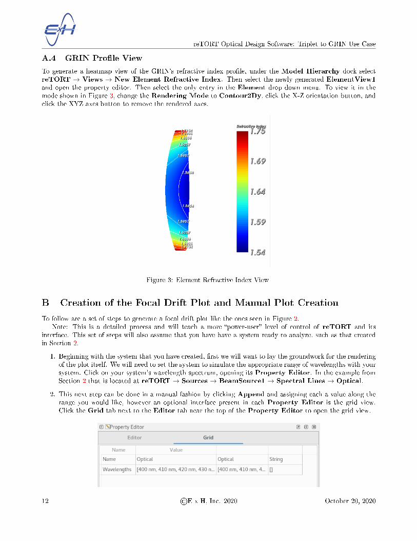
To generate a heatmap view of the GRIN's refractive index pro�le, under the Model Hierarchy dock selectreTORT → Views → New Element Refractive Index. Then select the newly generated ElementView1and open the property editor. Then select the only entry in the Element drop down menu. To view it in themode shown in Figure 3, change the Rendering Mode to Contour2Dy, click the X-Z orientation button, andclick the XYZ axes button to remove the rendered axes.

Figure 3: Element Refractive Index View

B Creation of the Focal Drift Plot and Manual Plot Creation

To follow are a set of steps to generate a focal drift plot like the ones seen in Figure 2.Note: This is a detailed process and will teach a more �power-user� level of control of reTORT and its

interface. This set of steps will also assume that you have have a system ready to analyze, such as that createdin Section 2.

1. Beginning with the system that you have created, �rst we will want to lay the groundwork for the renderingof the plot itself. We will need to set the system to simulate the appropriate range of wavelengths with yoursystem. Click on your system's wavelength spectrum, opening its Property Editor. In the example fromSection 2 that is located at reTORT → Sources → BeamSource1 → Spectral Lines → Optical.

2. This next step can be done in a manual fashion by clicking Append and assigning each a value along therange you would like, however an optional interface present in each Property Editor is the grid view.Click the Grid tab next to the Editor tab near the top of the Property Editor to open the grid view.

12 ©E x H, Inc. 2020 October 20, 2020


3. The grid view allows for more direct modi�cation of values in your system. The �rst column of the gridview lists the names of each property of the associated object. The second column is the region of the gridview that you will edit to change the values of the various properties. The third and fourth columns are theevaluated version of the entry in the Value column and the type of information respectively. It is importantto remember that when using this interface it is quite possible to invalidate your system by entering invalidinformation into these �elds. The Wavelengths entry is an array of values with units attached. You maymanually enter the set of wavelengths you wish to use here in the form of an array. The values used forFigure 2 were 30 nm increments from 400 nm to 700 nm or as follows:

[400 nm , 430 nm, 460 nm, 490 nm, 520 nm , 550 nm , 580 nm, 610 nm, 640 nm, 670 nm , 700 nm]

Enter this array into the Value column in the Wavelengths row. Your system is now set to simulatethese eleven wavelengths, which can take a while to simulate as there is a seperate set of rays for eachwavelength/incident angle combination. It is advised that you change this set of wavelengths back to theoriginal three after generating this plot as the system may not run quickly with so many rays to simulate.

4. An additional step is to generate a result that can be referenced to see the focal drift. Generate a newoptical output through the reTORT → Results → RayResult1 → Outputs → New OpticalOutputoption. Set the Focus Calculation Method property of the new output toMinimum RMS. Also makesure the Compute Spot Metrics property is checked, to enable the FocalPoint result.

5. Now to create the plot itself. In the Model Hierarchy, right-click on Views and select New 2D Plot.

6. The plot now requires a Trace. Traces are the interface for selecting which data you wish to representand in which ways you wish to represent it. Expand your newly created Plot2DView1 and right-click onPlot2DView1 → Traces. In this menu select New Trace.

13 ©E x H, Inc. 2020 October 20, 2020


7. Click on the newly created Trace1 to open its Property Editor. Next to the Data Selection �eld, clickEdit. This will open a dialog box for selecting the data you wish to render. Select reTORT → Results→ RayResult1 → OutputOutput1_FocalPoint, and click OK. This table contains the focal pointlocations and spot sizes.

8. For the plots shown in Figure 2, we used the z location of the focal planes described in step 7 and thewavelengths added to the system in step 3. This information is present in the result table selected in step 7,and we apply it here by setting the X-Data �eld to Wavelength and the Y-Data �eld to Pz.

9. To render the plot, run your simulation by right-clicking reTORT in the Model Hierarchy and clickingRun All. You can alternatively press F5 on the keyboard to do the equivalent. Furthermore, you can pressShift+F5 to clear all current data and re-run the system at any time.

14 ©E x H, Inc. 2020 October 20, 2020


10. By default, the Trace will have two seperate data sets rendered, one per incident angle.

To change this to match the plots in Figure 2, change the Theta �eld in the Property Editor of Trace1from Full to Single and drag the small slider to select the incident angle you wish to render. For the plotsin Figure 2, we used 0°.

11. You can also change the units displayed on each axis through the Property Editor for the plot itself,Plot2DView1 in this case. Many of the options presented in the Property Editor can also be accessedthrough context menus on parts of the plot. Right-click on the title for the y-axis on the plot, in this casePz (m) and change the units to µm. Then do the same for changing the scale of the x-axis, Wavelength,to nm.

15 ©E x H, Inc. 2020 October 20, 2020


Your plot should now look something like this:

This set of steps is a framework that can be used for rendering any of the data present in the results of yoursimulations.

16 ©E x H, Inc. 2020 October 20, 2020

reTORT Optical Design Software: Triplet to GRIN Use Case

Documents

Transcript of reTORT Optical Design Software: Triplet to GRIN Use Case