Rethinking the Monetary Theory of the Trade Cycle … the... · Rethinking the Monetary Theory of...

This paper is a work in progress. Please contact the author for an updated version. DO NOT QUOTE.

Rethinking the Monetary Theory of the Trade Cycle and the Great Depression*

William J. Luther† George Mason University

Abstract

Was the Great Depression preceded by a period of excessive monetary expansion? The answer to this question would provide support for either the Monetarist view of the Great Depression as it currently stands or a view that incorporates the Austrian analysis, but not both. In this paper, we question the original calculations by Friedman and Schwartz (1963), which have since become the orthodox position. First, we consider the aggregate price level between 1921 and 1929. Next, we consider the relevant components of the money supply. Finally, we calculate the monetary expansion. We find that the money supply increased by 54.77% from 1921 to 1929. Furthermore, the bulk of this expansion took place in the market for loanable funds. These results are wholly consistent with the Austrian Business Cycle theory. As a result, we suggest the current view of the Great Depression be modified to include monetary-induced malinvestment.

* We are very thankful for the comments provided by Lawrence H. White, Steven G. Horwitz, and Peter J. Boettke. We also thank the Mercatus Center at George Mason University for generously supporting this research. Any remaining errors are our own. † Email: [email protected] Address: Department of Economics, George Mason University, MSN 3G4, Fairfax, VA 22030

WORKING PAPER 1 Do Not Quote

I Introduction

During a 1934 radio broadcast John Maynard Keynes reflected on the intellectual

climate of the Great Depression, presenting two contrasting views among economists.1

The first, representative of the orthodoxy, regarded the economic system to be self-

adjusting, “though with creaks and groans and jerks, and interrupted by time lags, outside

interference and mistakes.” The second, whose supporters Keynes deemed heretics,

rejected this property altogether. And Keynes, of course, famously sided “with the

heretics.”

At present there are two fairly distinct schools of thought supporting the view of

the classical economists that the economy has a natural tendency to self-adjust. One

school was born as a challenger to Keynesian macroeconomics. The other existed prior

to Keynes and his General Theory. For simplicity, we label those following in the

tradition of Milton Friedman as Monetarists. Similarly, we refer to the intellectual

descendants of Knut Wicksell and Ludwig von Mises as Austrians.2 While both

emphasize the economic system’s self-adjusting properties and, further, the important

role money plays in generating a business cycle, they are in conflict with respect to the

fundamental cause of macroeconomic fluctuation. As such, their explanations of the

Great Depression differ significantly.

1 Available in Keynes, John M. The Collected Works of John Maynard Keynes. Edited by Donald Moggridge. Volume XIII, Part I, pages 485-492. 2 As Horwitz (2000, 77) explains, “the inflationary disequilibrium theory that emerged from Wicksell’s work was the Austrian theory of the business cycle in the hands of Mises and Hayek.” However, Mises (1949, 496) thought it “awkward indeed to attach to certain lines of thought national labels.” Perhaps ‘monetary malinvestment theory’ would be a better term.


The Austrian view holds that expansionary monetary policy in the 1920s

effectively increased the supply of loanable funds without actually increasing the amount

of savings to be lent. As a result, the loan rate of interest fell below the natural rate.3 At

the prevailing rate of interest, market participants invested in a more round about

structure of production.4 If increasing investment had been accompanied by an equal

increase in savings, the economy would have moved smoothly along. However, the

investment—which Austrian economists dub malinvestment—was fueled entirely by

monetary expansion.5 Since the total amount of investment and consumption is greater

than what is sustainable in the long run, the economy is driven into an artificial boom.

To clarify, below-market interest rates made ventures that would not have

otherwise been undertaken appear to be profitable. These investments diverted real

resources into specific forms of capital. Since resources are in scarce supply, the boom

could not last forever. Malinvestments were eventually realized to be unprofitable and,

in 1929, the boom came to a screeching halt.

The degree of specificity inherent in capital investments prohibits instantaneous

liquidation. As a result, the Austrian business cycle theory (ABCT) predicts a period of

recovery where the natural course of market correction takes place. Unprofitable assets

are reallocated to more productive ends. During this process, the aggregate economy

appears to be in a trough—output and employment are lower than their long-run, natural

3 The term ‘natural rate’ denotes that rate which would clear the market for actual savings and investment, articulating the time preferences of market participants. ‘Loan rate’ is defined as the prevailing rate in the market at a particular point in time. 4 The notion of roundaboutness in the Austrian tradition stems from Böhm-Bawerk (1890) and (1891). The intuition is clear: a lower interest rate increases the present discounted value of more distant payments and, therefore, leads to a longer time-structure of production. See also: Garrison (2001, 45-49) and Horwitz (2000, 40-61). 5 Malinvestment implies not only overinvestment but also a misallocation of capital.


levels.6 The depth and duration of a particular trough depend, among other things, on the

institutional framework and policy responses that facilitate (or prevent) to varying

degrees the weeding out of malinvestments.

In contrast with the Austrian view of a boom-bust cycle, Monetarists suggest

there is a bust-boom cycle.7 This position was originally articulated in Friedman and

Schwartz’s (1963) A Monetary History of the United States. They claim deviations in

output from the long-run trend occur when an inept or inexperienced central bank allows

the money supply to contract relative to output. This sudden contraction essentially pulls

the rug out from underneath the economy. Without enough money to facilitate the

volume of transactions desired, market agents are left consuming less until either the

price level adjusts downward or the money supply is increased. As a result, output and

employment fall. In the Monetarist view, the Federal Reserve (Fed) might have

prevented the Great Depression if it had not allowed the money supply to contract.8

That the Monetarist account has largely carried the day is arguably a function of

Friedman’s well-deserved academic reputation and the empirical support that he and

Schwartz, among others, have assembled. Austrian economists, on the other hand, have

provided relatively little empirical evidence for the ABCT.9 Furthermore, some early

expositors of the Austrian view were convinced that the ABCT alone could account for

6 In addition to total change in output, Garrison (1996, 799-800) emphasizes sectoral changes. 7 See: Friedman (1993) and Garrison (1996). 8 Friedman and Schwartz (1963, 299) observe that the stock of money fell by over a third from August 1929 to March 1933. 9 Using a more inclusive measure of the money supply than we are advocating, Rothbard (1963, 87-94) shows that the 1920s was a period of monetary expansion. Wainhouse (1984) tests for Granger causality and finds that movements in interest rates and relative prices are consistent with the ABCT. Butos (1993) finds support for the ABCT from the 1980s bull market.


the length and severity of the economic downturn, leaving no room for deflation as an

explanation (Selgin 1997, 58-59). For these reasons, modern economists have largely

rejected the monetary malinvestment theories out of hand.

Despite varying degrees of support, Austrian and Monetarist accounts of the Great

Depression are not irreconcilable.10 Accepting that a money-induced boom marked the

1920s does not require one to reject or reduce the role of deflation in prolonging the

economic downturn.11 As Garison (1996, 800-801) explains, the “market process that

liquidates the malinvestments is likely to involve complications—especially if the central

bank behaves counterproductively—that result in a substantial reduction in total output.

A self-aggravating, income-constrained process can entail an idling of capital and labor

far in excess of that made necessary by the intertemporal disequilibrium.” Similarly,

Selgin (1997, 58) notes that the monetary expansion “is only likely to have played a

relatively minor part in explaining the length and severity of the depression, in contrast to

its major role in causing the stock-market boom and crash.” While the boom was wholly

responsible for the bust, the aberrant depth and duration of the trough that followed was

surely a result of counterproductive policies. In this sense, Austrian and Monetarist

accounts are complementary.

With respect to complementarity, however, Friedman and Schwartz (1963, 298)

were quite clear that their evidence does not support the ABCT:

10 Garrison (1996, 800) emphasizes the similarities: “Although Austrians and Monetarists are working at different levels of aggregation, they are dealing with the selfsame macroeconomy, as evidenced by each school's recognition of the movements of output that constitute the other's primary concern. 11 In addition to contractionary monetary policy, Ohanian (Forthcoming) and Cole and Ohanian (2004) blame industrial labor policies under Hoover and Roosevelt, respectively, for the length and depth of the depression. Higgs (1997) claims regime uncertainty stifled the recovery. These ideas are also consistent with the Austrian view.


The economic collapse from 1929 to 1933 has produced much misunderstanding

of the twenties. The widespread belief that what goes up must come down and

hence also that what comes down must do so because it earlier went up, plus the

dramatic stock market boom, have led many to suppose that the United States

experienced severe inflation before 1929 and the Reserve System served as an

engine of it. Nothing could be further from the truth. By 1923, wholesale prices

had recovered only a sixth of their 1920-21 decline. From then until 1929, they

fell on the average of 1 percent per year. […] The stock of money, too, failed to

rise and even fell slightly during most of the expansion—a phenomenon not

matched in any prior or subsequent cyclical expansion. Far from being an

inflationary decade, the twenties were the reverse.

In this paper, we will reevaluate the claims of Friedman and Schwartz with respect to

aggregate price levels and the changing stock of money. First, however, we consider

whether Schwartz has changed her position since writing with Friedman.12

In addressing the “influences on the emergence of the global financial crisis,”

Schwartz (2009, 19) naturally points first to monetary factors. Surprisingly, her

account does not match up with the Friedman-Schwartz bust-boom cycle.

The basic groundwork to the disruption of credit flows can be traced to the asset

price bubble of the housing price boom. It has become a cliché to refer to an

asset boom as a mania. The cliché, however, obscures why ordinary folk

become avid buyers of whatever object has become the target of desire. An asset

12 Scott Sumner (2009) initially pointed out the apparent change in Schwartz’s position on his blog, The Money Illusion. Sumner claimed that, “[w]ere he alive today, Friedman would be horrified by the neo-Austrian views of Anna Schwartz.”


boom is propagated by an expansive monetary policy that lowers interest rates

and induces borrowing beyond prudent bounds to acquire the asset (Schwartz

2009, 19).

It seems that, at least with respect to the current crisis, Schwartz believes there was an

Austrian-style boom-bust cycle. This might be interpreted as evidence that Schwartz

has changed her position since writing with Friedman in the early 60s or alternatively

that the characteristics of this particular crisis differ from those of the Great Depression.

In an interview with the Wall Street Journal, however, Schwartz makes it clear that the

pertinent characteristics are the same.

If you investigate individually the manias that the market has so dubbed over the

years, in every case, it was expansive monetary policy that generated the boom

in an asset. The particular asset varied from one boom to another. But the basic

underlying propagator was too-easy monetary policy and too-low interest rates

that induced ordinary people to say, well, it's so cheap to acquire whatever is the

object of desire in an asset boom, and go ahead and acquire that object. And

then of course if monetary policy tightens, the boom collapses (Carney 2008).

According to Schwartz, the current crisis is not a special case: “every case,” presumably

including the Great Depression, is the result of a monetary-induced boom.

That Schwartz has seemingly changed her mind on the nature and causes of the

Great Depression is just one reason to reevaluate the empirical evidence. Additionally,

the policy recommendations of Monetarists and Austrians differ substantially: the former

argue that an additional expansion in the money supply is necessary, while the latter


advocate a more hands-off approach.13 Finally, a better understanding of the fundamental

causes of the business cycle might result in fewer or, at least, less severe fluctuations in

the future. In what follows, we attempt to critically evaluate data from the 1920s in order

to determine whether the Fed engaged in expansionary monetary policy.

In section II we consider various measures of the general price level in the period

and discuss the relevance of this particular type of measure with respect to the topic of

interest. Then, in section III, we define the money supply to include currency, demand

deposits, time deposits at commercial banks, savings accounts at mutual savings banks,

share accounts at savings and loan associations, and Postal Savings System deposits.

Given this definition, we find empirical support that the money supply increased

substantially from 1922-1929 in section IV. Finally, we offer concluding remarks in

section V.

II Price Level

Critics of the Austrian view of the Great Depression often point to the stable price

level throughout the 1920s as evidence of monetary stability. Austrians, on the other

hand, are skeptical that aggregate price levels convey the information necessary to make

such a claim. To be sure, both consumer and wholesale price indices depict little-to-no

change over the period. The level of aggregation, however, might be concealing

important facts.

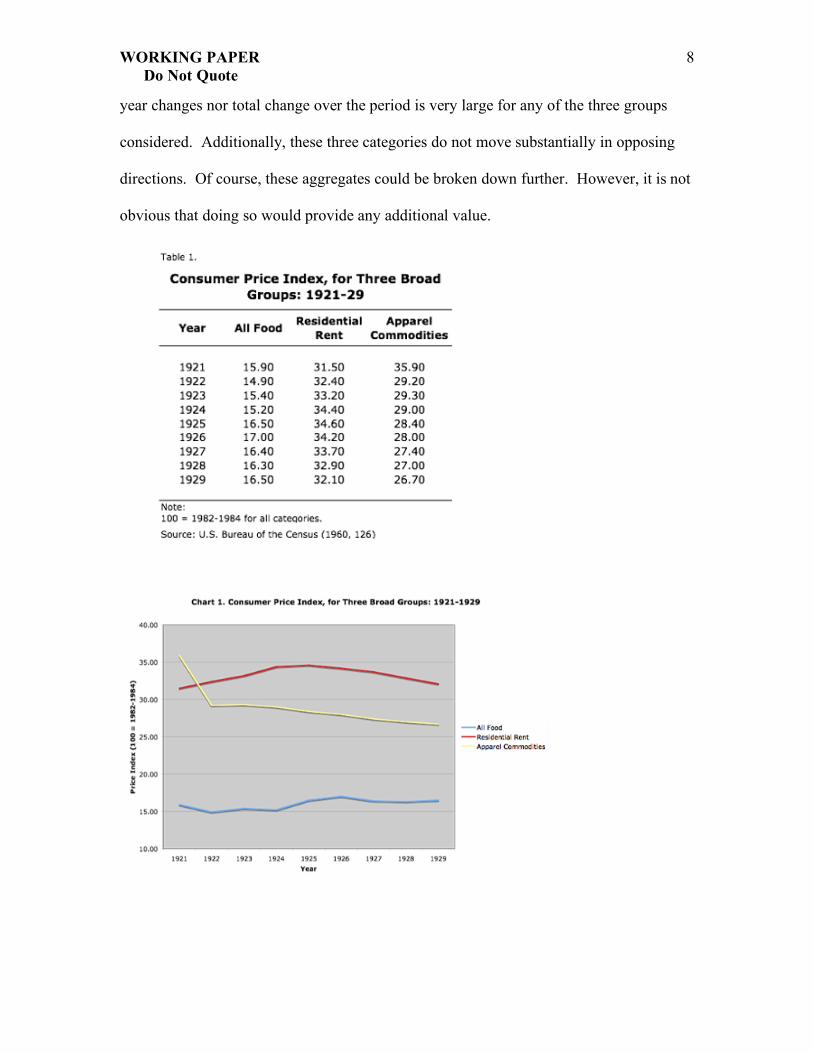
Disaggregating the consumer price index confirms that output prices were

relatively stable from 1922-1929. Table 1 presents the consumer price index, by three

broad groups; these three categories are graphically depicted in Chart 1. Neither year-to-

13 Recall that the Monetarists see the problem as a lack of liquidity while the Austrians note the necessity of clearing out malinvestment.


year changes nor total change over the period is very large for any of the three groups

considered. Additionally, these three categories do not move substantially in opposing

directions. Of course, these aggregates could be broken down further. However, it is not

obvious that doing so would provide any additional value.


In sharp contrast to the components of the consumer price index, the wholesale

price index disaggregated by stages of processing, as Table 2 and Chart 2 illustrate,

varied quite a bit from year-to-year. Chart 2 does not leave one with the impression that

wholesale prices smoothly “fell on the average of 1 percent per year” from 1922-1929, as

Friedman and Schwartz’s (1963, 298) suggest. The average price of raw materials

increased by 11.15% from 1922 to 1925. And in just one year, from 1922 to 1923, the

price of semimanufactured items shot up 19.92%. While both eventually fell back down

to near-1922 levels as the decade came to a close, it seems odd to proclaim that stable

prices were the norm. At least when arranged by stages of processing, the price level

seems to have been quite dynamic throughout the 1920s.


Disaggregating the wholesale price index by commodity groups, rather than

stages of processing, yields a result similar to the consumer price index. The price of

most commodities—excluding only ‘spirits’ and ‘hides and leather products’—fell more

or less smoothly over the period. It is probably appropriate to disregard the changing

price of spirits as it likely reflects measurement errors stemming from the legal status of

alcoholic beverages in the 1920s. Hides and leather products, the price of which moves in

the opposite direction, increased by 42.95% from 1926 to 1928. Nonetheless, it seems

reasonable to concede that wholesale prices—at least when viewed by commodity

groups—were relatively stable from year-to-year and throughout the period of interest.

Even if we were to agree that output prices were kept relatively constant across

sectors from 1922-1929, it does not necessarily follow that the period was one of

monetary stability. Technological progress, in absence of Fed policy, would likely result

in a gradual fall in the aggregate price level as cost-cutting production processes are

implemented.14 Assuming only a moderate amount of progress took place in the 1920s—

and it seems reasonable to think this was the case—we should expect to see a falling

price level. That we do not observe falling prices is evidence of monetary expansion.

The relevant concern, of course, is whether this expansion should be deemed ‘excessive’.

In other words, can active monetary policy that effectively stabilizes the aggregate price

level generate a boom-bust cycle?

14 Alternatively, a constant aggregate price level in the face of technological progress might also be observed if quality is improving and, hence, real prices are falling. Raff and Trajtenberg (1997) find that the quality-adjusted price of the average automobile fell roughly 27.14% from 1922 to 1928. However, it is unlikely that all productivity gains in all industries resulted exclusively in higher quality goods; some improvements surely resulted in a lower cost method of production for more or less the same quality good.


Selgin (1997, 39) claims “attempts to stabilize the price level in the face of

productivity shocks themselves become a source of disequilibrating monetary

misperception effects.” Similarly, Horwitz (2001, 69) argues that assuming the price

level adjustment spurred by monetary policy is costless ignores the very reason

policymakers attempt to avoid monetary disequilibrium in the first place. In reality,

money is injected into the economy at a particular point and spreads throughout the

economy only with the passage of time. Given that prices do not adjust instantaneously,

the flow of money alters the relative purchasing power of individual actors and, therefore,

changes relative prices along the way. As Board of Governors (1937, 827) notes:

No matter what price index may be adopted as a guide, unstable economic

conditions may develop, as they did in the 1920’s, while the price level remains

stable; business activity can change in one direction or the other and acquire

considerable momentum before changes are reflected in the index of prices.

There are situations in which changes in the price level work toward maintenance

of stability; declining prices resulting from technological improvements, for

example, may contribute to stability by increasing consumption.

Therefore, one might prefer a “productivity norm,” where “changes in velocity would be

prevented (as under zero inflation) from influencing the price level through offsetting

adjustments in the supply of money. But adverse ‘supply shocks’ like wars and harvest

failures would be allowed to manifest themselves in higher output prices, while

permanent improvements in productivity would be allowed to lower prices permanently

(Selgin 1997, 10).” At the very least, one must recognize that a stable aggregate price

level is insufficient evidence to claim monetary stability.


If we are to investigate the claim that monetary expansion in the 1920s fueled a

boom-bust cycle, we must look beyond aggregate price levels. In the next two sections,

we define the money supply and calculate the monetary expansion for the period in an

effort to see what is hidden behind the stable price level.

III Defining Money

Deciding what should count as money is no easy task. Consider the words of

Leland Yeager (1968, 45-69):

Of course, a broad definition of money is not downright “wrong” since many

definitions of money can be self-consistent. But no mere definition should deter

us, when we are trying to understand the flow of spending in the economy, from

focusing attention on the narrow category of assets that actually get spent. It is

methodological prejudice to dismiss as irrelevant, without demonstrating their

irrelevance, such facts as these: Certain assets do and others do not circulate as

media of exchange. No reluctance of sellers to accept the medium of exchange

hampers anyone’s spending it. The medium of exchange can ‘burn holes in

pockets’ in a way that near moneys do not […] These are observed facts, or

inferences from facts, not mere a priori truths or tautologies.

While Yeager’s urging of adherence to a simple definition of the money supply is

compelling, it loses some of its appeal once one points out that checks, which “actually

get spent,” are only accepted insofar as they can be converted into currency. 15 Checks

are valuable because market participants believe they can be converted at par and on

15 In the 1920s, market participants were not required to accept currency either. Only gold was deemed legal tender in the narrow sense that no one could refuse it as payment for debt. Therefore, we might also consider currency as near-money for this period. For our purposes, this distinction is unnecessary.


demand for currency.16 Checkable deposits, then, are merely a very close substitute for

currency. This opens the door for a much broader definition of the money supply.

Like Yeager, we take as the key function of money to be its use as a medium of

exchange. However, we are concerned with both currency and close substitutes. This

obviously raises a difficult question: with a wide range of possible components, where

does one draw the line? Simpson (1979, 17-18) suggests a second criterion for inclusion

when he asks if the asset is “readily convertible into a transaction balance,” that is, “Does

the public view it […] as a highly liquid alternative?” This subjectivist criterion meshes

well with the Austrian tradition. We include it in our definition of money.

Cargill (1979, 11) lists a spectrum of assets in terms of liquidity, or how quickly

and cheaply they can be converted into currency. We duplicate this list in Table 1. To

clarify, we designate the money supply to include those assets that are:

(1) Redeemable at par and on demand

(2) Considered to be highly liquid alternatives by market participants

Friedman and Schwartz (1970, 148) list six potential components of the money supply,

all of which are available at par and on demand: currency, demand deposits at

commercial banks, time deposits at commercial banks, deposits at mutual savings banks

and the Postal Savings System, savings and loan shares, and cash surrender value of life

16 Friedman and Schwartz (1970, 105) make a similar argument, noting that ten thousand dollar notes “can seldom be used directly as means of payment; they must first be converted into smaller denominations.” Nonetheless, large denomination bills are included in the stock of currency that Yeager and others deem the appropriate measure of money.


insurance policies.17 In what follows, we discuss whether these particular assets were

considered to be sufficiently close substitutes for currency in the 1920s.

Since no one contests the inclusion of currency and demand deposits, we start our

discussion by considering savings accounts. We do not make a clear distinction between

time deposits and savings accounts. This approach is not unique to us. The Board of

Governors (1943) categorized time deposits at commercial banks, accounts at mutual

savings associations, and Postal Savings System deposits under the same broad term:

time deposits. The observant reader will notice that time deposits follow savings

accounts in Table 4. However, the distinction and relative position of time deposits on

Cargill’s (1979, 11) spectrum of liquidity is disputable for the period we consider; it

largely reflects institutional changes that occurred long after the 1920s. Substantial

17 In addition to these components, Rothbard (1963) and Salerno (1987) include deposits held by the U.S. government. We are concerned exclusively with the holdings of the general public. Therefore, we exclude these numbers. We also note, however, that the inclusion of government deposits has virtually no effect on our conclusions. Government deposits totaled only $418 million in June 1921; they dropped to 381 million in June 1929 (Federal Reserve 1943, 34-35).


penalties for early withdrawal introduced in 1973 and a “steady lengthening of

maturities” made time deposits much less liquid (Simpson 1979, 13).18 This fact is best

illustrated by the Board of Governors’ (1943, 11) earlier claim that “time deposits and

demand deposits both represent similar bank liabilities and have similar roles in the

process of bank credit expansion or contraction.”19 Additionally, some time deposits were

subject to checking prior to 1932.20 Of course, checkable time deposits were still “less

active than demand accounts in the same banks, but much more active than other time

accounts in many sections of the country (Board of Governors 1931, 15).” Given that the

differences in time deposits and savings accounts were largely nominal in the 1920s, we

do not attempt to make a distinction between these assets and consider their inclusion

concurrently.

It is widely held that “during the 1920's time deposits at banks could be and were

more freely used for current payments than at other times (Board of Governors 1943,

11).” Hence, by the criteria outlined above, these accounts should be included in the

money supply. Establishing the orthodox position, Friedman and Schwartz (1963)

include time deposits at commercial banks; they do not include savings accounts at

18 See also: Berkman (1980, 137). 19 See also: Federal Reserve Board (1941, 302). 20 Admittedly, it seems odd that time deposits would be transferable by check. Friedman and Schwartz (1970, 156) explain: “The relative costs to banks of supplying the two kinds of liabilities have differed greatly among groups of banks at any one time and for any one group of banks over time. As a result, banks have had, to a varying degree at different times, incentives to enhance or reduce the relative attractiveness of time deposits to their depositors, and they have done so at least in part by changing the characteristics of deposits labeled as ‘time’ so as to make them either more like or less like deposits labeled ‘demand.’ The introduction in the Federal Reserve Act of lower reserve requirements for time deposits than for demand deposits gave member banks an incentive to persuade their depositors to hold time deposits rather than demand deposits. Nonmember banks initially had no such incentive, though as time went by some states altered their laws to match the federal law.”


mutual savings banks, deposits at the Postal Savings System, or share accounts of savings

and loan associations. There are several possible reasons for omitting these accounts.

We address each in turn.

One might choose to exclude savings and loan shares and Postal Savings System

deposits because these institutions were not technically banks. While the latter is clearly

not a bank, a subtle legal distinction excludes the former as well. To put it simply, those

entrusting their funds to savings and loan associations were not legally defined as

depositors, but rather shareholders. On this issue, Friedman and Schwartz (1963, 4) state

the following:

We consider a financial institution to be a bank if it provides deposit facilities for

the public, or if it conducts principally a fiduciary business—in accordance with

the definition of banks agreed upon by federal bank supervisory agencies. Of

these two classes, fiduciaries are negligible in importance. Banks are classified as

either commercial or mutual savings banks. Commercial banks include national

banks, incorporated state banks, loan and trust companies, stock savings banks,

industrial and Morris Plan banks if they provide deposit facilities, special types of

banks of deposit—such as cash depositories and cooperative exchanges in certain

states—and unincorporated or private banks. Mutual savings banks include all

banks operating under state banking codes applying to mutual savings banks.21

Of course, this would not explain why mutual savings banks are omitted, as they were

explicitly deemed banks under this legal definition.

21 Friedman and Schwartz (1970) explain their approach to defining the money supply in great detail. On page 75, they include this definition again.


We are hesitant to throw out share accounts of savings and loan associations

because there happens to be a legal distinction between these institutions and depository

institutions, particularly considering that Friedman and Schwartz (1963, 4) recognize

market actors “may regard such funds as close substitutes for bank deposits.” 22 Savings

and loan associations received funds from the public in order to make loans and

investments in much the same way as depository institutions. Similarly, they were

contractually obligated to repurchase shares at par and on demand.23 Furthermore, the

M2 measure of the money supply has included share accounts since 1980.24

A similar argument could be made for the Postal Savings System. Established

January 1, 1911, the Postal Savings System primarily functioned as an alternative savings

option for “immigrants accustomed to saving at Post Offices in their native countries”

and those “who had lost confidence in banks” (US Postal Service 2008). Deposits paid

two percent annual interest and most deposits were redeposited in local banks. Although

there was a clear legal distinction, we find that savings and loan associations and the

22 Friedman and Schwartz (1970, 75) repeat this word for word. 23 As Salerno (1999, 33) notes, savings and loan associations “could legally delay such repurchase for shorter or longer periods depending on their individual bylaws” in much the same way as “the law […] permitted banks to insist on a waiting period.” In practice, however, both organizations paid withdrawals on demand. 24 We are obligated to note that the Depository Institutions Deregulation and Monetary Control Act of 1980 allowed savings and loan associations to offer checkable deposits. Additionally, Simpson (1979, 15) lists several developments in the 1970s that may have affected the nature of monetary aggregates including negotiable order of withdrawal accounts, automatic transfer services, and payment order accounts. To the extent that these changes led to the inclusion of savings and loan shares in the M2, their inclusion does not support our position. Even still, we contend that share accounts and savings accounts were sufficiently similar in the 1920s such that if the inclusion of one is justified, the other follows naturally.


Postal Savings System were economically indistinguishable from those institutions

legally defined as banks.25

Practical concerns may also warrant excluding savings and loan shares. As

Friedman and Schwartz (1970, 171) note, savings and loan data is only available for part

of the period they were considering. Since the data is available back to 1897, this is of

not pertinent to our study. Another problem with savings and loan data is the infrequency

with which it was reported. While monthly totals are available for most other accounts in

the period, savings and loan shares were only reported in December. We reject the idea

that savings and loan shares were excluded for statistical reasons. The data seems

sufficiently reliable. Furthermore, Friedman and Schwartz (1970, 171) claimed these

considerations “played no role” in decision to omit savings and loan associations.

One might argue Postal Savings System deposits were of little economic

significance in the 1920s. The maximum balance of each account was held to $2,500 and

in June 1921 less than $150 million were in the Postal Savings System. This total fell to

$131 million by 1923 and did not recover to its 1921 level for six years. To be sure,

these deposits made up a very small percentage of the money supply and the total amount

held in the Postal Savings System was relatively stable for the period. Given that the data

is readily available, though, we see no reason to exclude these deposits.

Friedman and Schwartz (1970, 175-176) also note the potential of a geographic

bias with mutual savings associations and savings and loan associations. The former only

operated in eighteen states and the latter, while available in all states, were heavily

25 The Postal Savings System officially closed on July 1, 1967 (U.S. Postal Service 2008). By 1980, savings and loan associations were recognized as depository institutions (Simpson 1980, 98).


concentrated in California, Illinois, Ohio, and New York.26 While this is obviously a real

concern, the bias would result from either including these accounts when they should not

be included or excluding them when they should be included. The potential bias gives no

indication as to whether one should include these accounts, but rather emphasizes the

importance of making the right decision. Therefore, the choice to include or exclude

these accounts must find its motivation elsewhere.

Despite the reasons offered above, the most likely explanation for omitting mutual

savings accounts, Postal Savings System deposits, and savings and loan share accounts is

that they correlate less strongly with GDP than commercial deposits (Friedman and

Schwartz 1970, 177).27 Admittedly, though, the empirical evidence is a mixed bag. While

Laumus (1968) upholds the orthodox view, Timberlake and Fortson (1967) find support

for a more narrow definition including only currency and demand deposits. Chetty

(1969) finds that time and savings deposits at mutual savings banks and savings and loan

associations possess a lesser degree of ‘moneyness’ than those at commercial banks, but

concludes that they are sufficiently liquid to warrant inclusion in the monetary

aggregate.28 Similarly, Lee (1966, 456) reports statistical results that “do not support

26 In December 1966, forty-one percent of savings and loan shares were held in these four states; in comparison, the four states holding the largest amounts of commercial bank deposits (New York, California, Illinois, and Pennsylvania) held only thirty-five percent of total deposits (Friedman and Schwartz 1970, 176). 27 More correctly, the criterion was that the correlation between all components included in a particular measure of the money supply and national income was greater than the correlation between any single component of the total and national income. See footnote 21 in Friedman and Schwartz (1970, 171). 28The varying degrees of liquidity have led Barnett (1980), Rotemberg et al (1995), and others to suggest various weighted monetary aggregates. See also: Moroney and Wilbratte (1976)


Friedman’s rationale for his particular definition of money.”29 One obvious concern with

these studies is that they focus on different time periods. Since financial regulations

changed over time, it is possible that what was once regarded as highly substitutable is no

longer so or vice versa. Furthermore, it is not entirely clear why one should judge the

fruitfulness of a definition solely on the basis of statistical correlation, which may or may

not reflect the subjective beliefs of market participants.

In the absence of empirical consensus, we resort to the definition proposed above.

Restricting the money supply to include only time deposits at commercial banks, demand

deposits, and currency is insufficient; we must also include mutual savings accounts,

Postal System Savings deposits, and share accounts at savings and loan associations. All

of these accounts are redeemable at par and on demand. Additionally, there is reason to

believe market participants viewed these assets as sufficiently liquid substitutes.

While Cargill (1979, 11) lists many assets with lesser degrees of liquidity, he

points out “few argue that financial assets beyond savings and time deposits should be

included in defining the money supply.” Large certificates of deposits were included in

the definition of M3. However, the Federal Reserve discontinued the M3 in 2006,

claiming that it “does not appear to convey any additional information about economic

activity that is not already embodied in M2 and has not played a role in the monetary

policy process for many years (Board of Governors 2005).” Additionally, it seems

reasonable to suspect that market participants did not consider these assets to be

sufficiently close substitutes for currency in the 1920s.

29 Lee (1966, 455) goes so far to claim “savings and loan shares appear to be better substitutes for demand deposits than do time deposits.” Friedman and Schwartz (1970, 181-184) offer a lengthy response and conclude by claiming “Lee has grossly overstated the economic significance of his calculations.” See also: Tobin (1965).


Even more controversial is the potential of including reserves of life insurance

companies. As Table 4 illustrates, these assets are less liquid than large certificate

deposits. Nonetheless, Haines (1961, 249-50) classifies insurance companies as “savings

institutions” and points out that they are redeemable at par and on demand by allowing

the policy to lapse.30 Burstein (1963, 111) provocatively claims they are “almost as

liquid as a mattress of currency.” Surely this is a bit of an exaggeration. Hart and Kenen

(1961, 4-6) agree that they possess certain qualities of money, but only include them in

the broadest class of financial assets. Rothbard (1963, 90-91), who includes net policy

reserves in his measure of the money supply, notes that “the policyholder is discouraged

by all manner of propaganda from cashing in his claims, and that the life insurance

company keeps almost none of its assets in cash—roughly between one and two percent.”

As such, it seems a bit contrived to suggest market participants looked on reserves of life

insurance companies as sufficiently liquid alternatives. We do not include them in our

measure of money.

To summarize, we find the following assets to be sufficiently liquid to be viewed

as apparent substitutes for currency by market participants: demand deposits, time

deposits at commercial banks, savings accounts at mutual savings banks, share accounts

at savings and loan associations, and Postal Savings System deposits. We do not include

large certificates of deposits or reserves of life insurance companies. Nor do we include

any of the other less liquid assets listed in Table 4.

IV Data

Description of the Data

30 Recall that Friedman and Schwartz (1970, 148) also recognize that net policy reserves were available at par and on demand.


Having established what counts as money, we now proceed to measure the money

supply. Table 5 reports our calculation of the money supply by components from 1921-

1933. In addition to the measure we endorse, we include totals for alternative measures

for comparison. Columns 1-5 are reproduced from Board of Governors (1943, 34-35).

Savings and loan balances, presented in column 6, are taken from Friedman and Schwartz

(1970, 18-28). These sources discuss in detail how the respective columns were

calculated. In what follows, we merely describe the data presented in Table 5.

Currency outside banks. Column 1 shows, as nearly as possible, the amount of

currency held by the public. Since currency held as vault cash is not held by the public,

this amount has been deducted from the total amount of currency outside the Treasury

and Federal Reserve Banks.

Demand deposits adjusted. All demand deposits at commercial banks in the

continental United States except interbank and United States Government deposits are

included in column 2. To prevent double counting, cash items in the process of being

collected have been excluded. The summation of columns 1 and 2 are presented in

column 7.

Savings accounts. All time deposits held at commercial banks except interbank

deposits, postal savings redeposited in banks, and United States Government time

deposits are included in column 3. The summation of columns 7 and 3 are presented in

column 8. Column 4 includes deposits held at mutual savings banks.31 Post Office

31 Relatively small amounts of demand deposits are inevitably included in this column. Theoretical concerns warrant removing these deposits. Unfortunately, this is a limitation of our data set that cannot be overcome. Given that our definition of the money supply includes both demand and time deposits, this problem is of little consequence to our conclusion.


Department figures for depositors' balances in the Postal Savings System are included in

column 6, including those amounts redeposited in banks as well as those amounts not so

redeposited. Amounts redeposited in banks outside the continental United States are

excluded. Deposits at savings and loan associations, adjusted to prevent double counting,

are included in column 6. June estimates are interpolated between reported December

balances. Columns 1-6 are summed and presented in column 9, the total money supply.

Results

If the 1920s boom were monetary-induced, as Austrians claim, we would expect

the money supply to increase during the period of the alleged boom. As presented in

Table 5, the money supply in June 1921 totaled roughly $39.16 billion. In June 1929, the

money supply had expanded to $60.61 billion, a 54.77% increase from the 1921 level.

This amounts to an average annual inflation of 6.85% over the eight-year period.

The major increases took place between June 1922 and June 1923 (9.58%), June

1924 and December 1925 (13.9%, 9.27%), and June to December 1927 (3.75%, 7.5%).32

Furthermore, the growth in money came to a screeching halt precisely as predicted

between December 1928 and June 1929 (-0.51%, -1.02%).

Even more significant than the overall growth in the money supply is the fact that

the bulk of this growth took place in the market for loanable funds. Savings and loan

shares increased by roughly $4 billion, from $1.79 billion in 1921 to $5.82 billion in

1929. Time deposits at commercial banks increased by $8.64 billion, approximately 79%

of the 1921 level. Similarly, mutual savings deposits increased by more than 61% over

the period, an absolute difference of $3.39 billion. That these accounts increased by

32 The first number in parentheses indicates total percentage change over the period, whereas the second is the average annual percentage change.


$16.06 billion while demand deposits increased by a mere $5.7 billion and currency

outside of banks remained relatively constant lends support for the Austrian view that

most of the monetary expansion took place in the credit market, generating a substantial

amount of malinvestment in the period.

Robustness

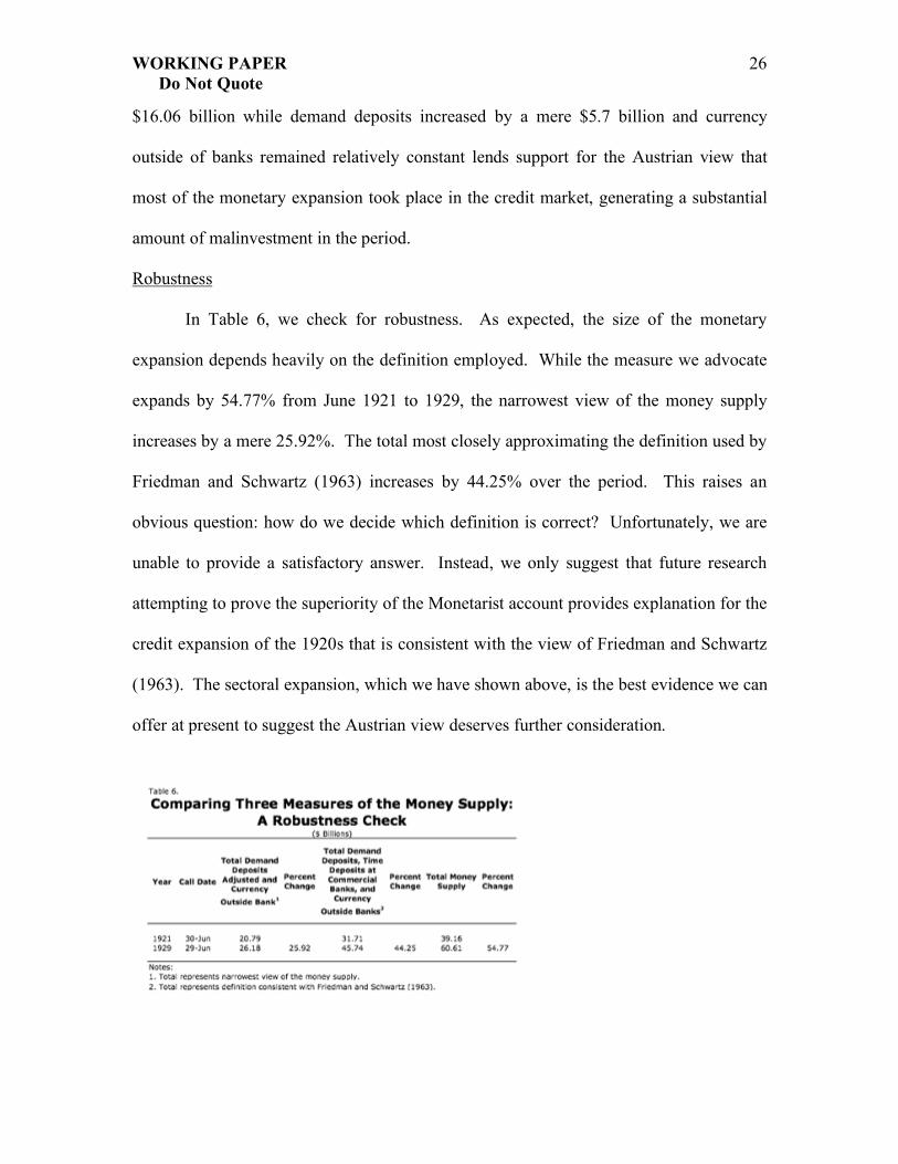
In Table 6, we check for robustness. As expected, the size of the monetary

expansion depends heavily on the definition employed. While the measure we advocate

expands by 54.77% from June 1921 to 1929, the narrowest view of the money supply

increases by a mere 25.92%. The total most closely approximating the definition used by

Friedman and Schwartz (1963) increases by 44.25% over the period. This raises an

obvious question: how do we decide which definition is correct? Unfortunately, we are

unable to provide a satisfactory answer. Instead, we only suggest that future research

attempting to prove the superiority of the Monetarist account provides explanation for the

credit expansion of the 1920s that is consistent with the view of Friedman and Schwartz

(1963). The sectoral expansion, which we have shown above, is the best evidence we can

offer at present to suggest the Austrian view deserves further consideration.


V Conclusion

The Austrian Business Cycle Theory claims that expansionary monetary policy

increases the supply of loanable funds without increasing the amount of savings to that

level which would be necessary to sustain the new, higher level of investment. As a

result, the economy enters an artificial boom period that inevitably results in a bust. In

contrast to the Monetarist account, which stresses a lack of liquidity, Austrians view

recessions as a period of market correction where malinvested resources are reallocated

to more productive ends.

Whether fluctuations in aggregate output exemplify the boom-bust cycle of the

Austrians or the bust-boom cycle of the Monetarists is an empirical question. With

respect to the Great Depression, we have shown that the money supply expanded

substantially in the 1920s. Additionally, we provide evidence that this expansion was

most pronounced in the market for loanable funds. However, our results are not robust;

they depend heavily on how one defines the money supply. Even still, we have offered

an alternative view of the Great Depression emphasizing the credit boom of the 1920s. If

nothing else, our paper warrants future research empirically evaluating the differences in

Austrian and Monetarists accounts with respect to the origins of macroeconomic

fluctuations.

References Barnett, William A. 1980. “Economic Monetary Aggregates: An Application of Index

Number and Aggregation Theory.” Journal of Econometrics. 14 (1): 11-48. Berkman, Neil G. 1980. “The New Monetary Aggregates: A Critical Appraisal.” Journal

of Money, Credit and Banking. 12 (2): 135-154. Böhm-Bawerk, Eugene. 1890. Capital and Interest: A Critical History of Economical

Theory. William A. Smart, trans. London: McMillan and Co. Available online: <http://www.econlib.org/library/BohmBawerk/bbCI.html>.


Böhm-Bawerk, Eugene. 1891. The Positive Theory of Capital. William A. Smart, trans. London: McMillan and Co. Available online: <http://www.econlib.org/library/BohmBawerk/ bbPTC.html>.

Burstein, Meyer L. 1963. Money. Cambridge, Mass: Schenkmann. Butos, William N. 1993. “The 1990-91 Recession and Austrian Business Cycle Theory:

An Empirical Perspective.” Critical Review, Spring-Summer: 277-306. Carney, Brian M. 2008. “Bernanke is Fighting the Last War.” Wall Street Journal.

October 18. Available online: <http://online.wsj.com/article/SB122428279231046053.html>.

Chetty, V. Karuppan. 1969. “On Measuring the Nearness of Near-Monies.” American Economic Review. 59 (3): 270-281.

Cole, Harold L. and Lee E. Ohanian. 2004. “New Deal Policies and the Persistence of the Great Depression: A General Equilibrium Analysis.” Journal of Political Economy, 112 (4): 779-816.

Board of Governors of the Federal Reserve System. 1931. “Report of the Committee on Member Bank Reserves.” Washington, DC: Federal Reserve.

Board of Governors of the Federal Reserve System. 1937. “Objectives on Monetary Policy.” Federal Reserve Bulletin, 23(9): 827-828.

Board of Governors of the Federal Reserve System. 1941. “Money System of the United States.” Banking Studies. 295-319. Washington, DC: Federal Reserve.

Board of Governors of the Federal Reserve System. 1943. Banking and Monetary Statistics 1914-1970. Washington, DC: Federal Reserve. Available online: <http://fraser.stlouisfed.org/publications/bms/>.

Board of Governors of the Federal Reserve. 2005. “Discontinuance of M3.” Federal Reserve: Washington, DC. Available online: <http://www.federalreserve.gov/Releases/h6/discm3.htm>.

Friedman, Milton and Anna Schwartz. 1963. A Monetary History of the United States, 1867-1960. Princeton: NBER and Princeton University Press.

Friedman, Milton and Anna Schwartz. 1970. Monetary Statistics of the United States: Estimates, Sources, Methods. New York: NBER and Columbia University Press.

Friedman, Milton. 1993. "The 'Plucking Model' of Business Cycle Fluctuations Revisited." Economic Inquiry. 31 (2): 171-77.

Garrison, Roger. 1996. “Friedman’s ‘Plucking Model’: Comment.” Economic Inquiry. 34 (4): 799-803.

Garrison, Roger. 2001. Time and Money: The Macroeconomics of Capital Structure. London: Routledge.

Haines, Walter A. 1961. Money, Prices and Policy. New York: McGraw-Hill. Hanes, Christopher. 1998. “Consistent Wholesale Price Series for the United States,

1860-1990.” Trevor J. O. Dick, ed. Business Cycles since 1820: New International Perspectives from Historical Evidence. Cheltenham, UK: Edward Elgar.

Hart, Albert G. and Peter B. Kenen. 1961. Money, Debt, and Economic Activity. Englewood Cliffs, NJ: Prentice-Hall.

Higgs, Robert. 1997. “Regime Uncertainty: Why the Great Depression Lasted So Long and Why Prosperity Resumed after the War.” Independent Review, 1 (4): 561-590.


Horowitz, Steven. 2000. Microfoundations and Macroeconomics: An Austrian Perspective. London: Routledge.

Keynes, John M. 1934. “Poverty and Plenty: is the economic system self-adjusting?” Radio broadcast. Donald Moggridge, ed. The Collected Works of John Maynard Keynes, 13(1): 485-492.

Laumus, G. S. 1968. “The Degree of Moneyness of Savings Deposits.” American Economic Review. 58 (3): 501-503.

Lee, Tong H. 1966. “Substitutability of Non-Bank Intermediary Liabilities for Money: The Empirical Evidence.” Journal of Finance. 21 (3): 441-457.

Mises, Ludwig von. 1949 (1996). Human Action: A Treatise on Economics. San Francisco: Fox & Wilkes.

Moroney, John R. and Barry J. Wilbratte. 1976. “Money and Money Substitutes: A Time Series Analysis of Household Portfolios.” Journal of Money, Credit, and Banking. 8 (2): 181-198.

Ohanian, Lee E. Forthcoming. “What—or Who Started the Great Depression?” Journal of Economic Theory.

Raff, Daniel M. G. and Manuel Trajtenberg. 1997. “Quality-Adjusted Prices for the American Automobile Industry: 1906-1940.” Timothy F. Bresnahan and Robert J. Gordon, eds. The Economics of New Goods. Chicago: University of Chicago Press.

Ranlett, John G. 1969. Money and Banking: An Introduction to Analysis and Policy. New York: John Wiley & Sons, Inc.

Rotemberg, Julio J., John C. Driscoll, and James M. Poterba. 1995. “Money, Output, and Prices: Evidence from a New Monetary Aggregate.” Journal of Business & Economic Statistics. 13 (1): 67-83.

Rothbard, Murray N. 1963 (2000). America’s Great Depression. Auburn: Mises Institute. Salerno, Joseph T. 1987. “The ‘True’ Money Supply: A Measure of the Supply of the

Medium of Exchange in the U.S. Economy.” Austrian Economics Newsletter, 6 (4): 1-6.

Salerno, Joseph T. 1999. “Money and Gold in the 1920s and 1930s.” The Freeman. 49 (10): 31-40.

Selgin, George. 1997. Less Than Zero: The Case for a Falling Price Level in a Growing Economy. London: Institute of Economic Affairs.

Simpson, Thomas D. 1979. “A Proposal for Redefining the Monetary Aggregates.” Federal Reserve Bulletin, 65 (1): 13-42.

Simpson, Thomas D. 1979. “A Redefined Monetary Aggregates.” Federal Reserve Bulletin, 66 (2): 97-114.

Sumner, Scott. 2009. “Friedman and Schwartz vs. the Austrians.” The Money Illusion. February 17. Available online: <http://blogsandwikis.bentley.edu/themoneyillusion/?p=203>.

Timberlake, Richard H. and James Fortson. 1967. “Time Deposits in the Definition of Money.” American Economic Review. 57 (1): 190-194.

Tobin, James. 1965. “The Monetary Interpretation of History.” The American Economic Review, 55 (3): 464-485.


Wainhouse, Charles. 1984 “Emperical Evidence for Hayek's Theory of Economic Fluctuations.” Money in Crisis: The Federal Reserve, the Economy, and Monetary Reform. Barry N. Siegel, ed. Cambridge, MA: Ballinger.

United States Bureau of Labor Statistics. 1957. “Wholesale Prices and Price Indexes.” Bulletin, 1,235.

United States Bureau of the Census. 1960. “Consumer Price Indexes (BLS), by Major Groups and Subgroups:1890-1957.” Historical Statistics of the United States, Colonial Times to 1957. Washington, D.C.

United States Postal Service. 2008. “Postal Savings System.” Available online: <http://www.usps.com/postalhistory/_pdf/PostalSavingsSystem.pdf>.

Wainhouse, Charles, E. 1984. “Empirical Evidence for Hayek’s Theory of Economic Fluctuations.” Money in Crisis: The Federal Reserve, the Economy, and Monetary Reform. Barry N. Siegel, ed. San Francisco: Pacific Institute for Public Policy Research.

Yeager, Leland. 1968. “Essential Properties of the Medium of Exchange.” Kyklos. 21 (1): 45-69.

Rethinking the Monetary Theory of the Trade Cycle … the... · Rethinking the Monetary Theory of...

Documents

Transcript of Rethinking the Monetary Theory of the Trade Cycle … the... · Rethinking the Monetary Theory of...