Retaining Wall Design-An Example of Small-Scale Optimization B. B. SCHIMMING, University of Notre Dame, and J . F. FISCHER, Sverdrup & Parcel and Assoc . , Inc., St. Louis

The feasibility of the application of optimization techniques to relatively small civil engineering problems as typified by re­taining wall design is presented. The objective function as mea­sured by the cost of concrete and reinforcing steel is mini­mized with respect to the toe, heel, stem base and footing thick­ness dimensions .

Four different numerical search techniques are employed in conjunction with a digital computer. They include: an ex­haustive search, the converging gradient ascent, the steepest ascent and the random search methods. The relative efficien­cies of the various approaches are discussed and compared.

Based on computer running time and programming effort required, it would appear that the state of the art has reached the point where very little additional expenditure is required in order to optimize the design of certain types of relatively small, common civil engineering problems.

•THE advent of the space age has injected a number of particularly meaningful words into the engineering vocabulary . In particular, the words system and optimum are two of the most commonly encountered. Confronted with vast projects composed of many inter­related components (system) involving huge expenditures of capital, the designer found it necessary and justifiable to consider the most efficient (optimum) configuration. The accumulated knowledge from this trend in conjunction with the general availability of digital computers has made it possible to examine the feasibility of applying optimal design to smaller systems.

U a physical system exhibits a structure which can be represented by a mathemnti­cal model, and if the value or merit of the system ca.11 be quantified as a function of the design variables, then some algorithm may be evolved for choosing the "best" answer. This procedure is generally referred to as mathematical programming.

The general programming problem seeks to minimize or maximize an objective function for n variables:

z = f(xj ) ; j = 1, . . . n

subject to m inequality or equality constraints,

gi (Xj) ~ = s: bi; i = 1, m

j = 1, n

with feasible solutions

Xj ~ 0 j = 1, ... n

In other words, the vector of independent variable values which yields the largest or smallest value of the objective function is sought within the region bounded by constraints.

Paper spon_!ored by Committee on Mechanics of Earth Masses and Layered Systems and presented at the 47th Annual Meeting.

44

45

As in most areas of analysis, the first successful approach to the general program­ming problem involved the linear case which can be stated as follows: f(xj) is a linear combination of the variables Xj and each g1(x·) is also a linear transformation. The algorithm, referred to as the simplex method., for solving the linear programming prob­lem was first introduced by G. B. Dantzig (1) in 1948.

The second important class of programming problems falls under the heading of non­linear programming. In this case f(X;) or at least one gi(JC_j) is nonlinear in at least one Xj. The nonlinearity, as might be suspected, considerably increases the difficulty of obtaining a solution. A number of relatively formal methods have been proposed to solve the nonlinear case (2, 3, 4) .

Often it may be necessary-to-resort to a numerical approximation when confronted with a nonlinear programming problem. Conceptually, the numerical approach is usual­ly easier, yet computationally more demanding.

In order to examine the present feasibility of relatively small design optimization, three different numerical approaches were applied to a typical nonlinear civil engineer­ing design problem-retaining wall design. The normal design of retaining walls using a digital computer has been previously discussed by Wadsworth(~).

PROBLEM DEFINITION

The type of retaining wall chosen for analysis is shown in Figure 1. It is basically a cantilever wall with no key. The height of the wall (H) above subgrade, including the required depth (D) to avoid frost action, and the thickness of the stem at the top (TT) are given dimensions, along with the slope of the soil behind the wall and the necessary soil properties. The remaining four dimensions are taken as the design variables:

TB = thickness of stem at bottom, TOE = toe length,

HEEL = heel length, and B = base thickness.

There are many constraints which a cantilever retaining wall must satisfy, the first one being stability. Both overturning and sliding stability must be considered, with a

minimum allowable factor of safety specified. The stability constraints

H

SLOPE ~ h/v used are those presented by Peck, Hanson and Thornburn (6) for a 1-ft length of wall. The remaining con­straints are all of the requirements dictated by the American Concrete Institute Building Code Requirements

D B

HEEL . I Figure 1. Cantilever retaining wall, no key.

for Reinforced Concrete - ACI 318-637. The objective function measures

the volume of concrete and the weight of reinforcing steel per lineal foot of wall and multiplies these values by their respective unit costs. The unit cost of ready-mix concrete and rein­forcing steel are those for St. Louis, Missouri, obtained from a recent issue of Engineering News-Record (8).

Examination of the constraints and the objective function indicates that the retaining wall problem is nonlinear . For example, the cross sectional area of the footing involves products of the design variable thus resulting in a nonlinear combination. In addition, the objective function is not explicitly

46

Definition

Stem thickness at top, in. Total heleht, ft

TABLE 1

INPUT DATA

Slope of soil surface behind wall Soil depth In front of wall, ft K-sub-V, ksf, (kv) K-sub-H, ksf, (kh) Unit weight of soil, kcf Unit weight of concrete, kcf Allowable soil pressure, ksf Friction between soil and base, ksf Overturning factor of safety Sliding factor of safety Compressive strength of concrete, psi Allowable steel tensile stress, ksi Allowable concrete shear stress, psi Modular ratio N, E(steet)/ E(concrete) Balanced design J Balanced design R, psl Uni t pr ice of re -bars, $ /100 lb Unit price of ready-mix, $/cu yd

Bar Size

3 4 5 6 7 8 9

10 11

Bar Diameter

(in.)

0. 375 o. 500 0.625 0,750 o. 875 1.000 1.128 1. 270 1. 410

Bar Area (sq in)

0.11 0. 20 0. 31 0.44 0. 60 0. 79 1.00 1. 27 1. 56

Symbol

TT H Slope D VK HK GS GC QA SF OFS SFS FC FS FSH EN FJ ARE us UC

Bar Perimeter

(in.)

1. 178 1. 571 1,963 2. 356 2. 749 3.142 3. 544 3.990 4.430

Value

12.000 16. 500 3.000 3.500 0.009 0.033 0.125 0.150 3.000 0. 550 1. 500 1. 500

3750. 0 24.000 67.000

8.250 0.8781 271.00 9,850

13. 500

Bar Weight (lb/ ft)

0.376 0.668 1. 043 1.502 2.044 2.670 3.400 4.303 5. 313

expressed in terms of the design variables. These conditions strongly suggest the use of nu­merical optimization techniques.

The input data, design vari­ables, constraints and objective function information are summa­rized in Tables 1 through 3. The actual wall to be optimized was again chosen from Peck, Hanson and Thornburn thus providing the input data. The concrete and steel specifications in the problem were replaced by the most recent reinforced concrete code and the reinforcing steel proper ties wer e those of standard deformed bars (ASMT A15, A305).

METHODOLOGY

Essentially, three different search techniques were pursued for the purpose of comparing their relative efficiency for this type of application. In addition, an exhaustive search which ex­amined all possible outcomes was conducted as a reference base.

A brief introduction to the three search methods is pre­sented for explanatory purposes;

however, the interested reader should consult a reference such as Wilde (9) to become aware of the pitfalls and limitations of each of the approaches. -

The response surface is a plot of the objective function versus the independent vari­ables . For the retaining wall problem the response surface would be a 5-dimensional plot of cost versus the 4 variable distanctH,l. The criterion for the existence of a maxi­mum or minimum in an n + 1 dimensional space is that the gradient

TABLE 2

VA R.J_A'RT.F.S• !l_~NGES A Nn TNr.RF.MF.N'T'S

Integer Increment Range Corresponding

Variable Associated Size for of Range oi With

Variable Variable Associated Variable Integer

TB 1TB 1. 00" 13"-30" 1-18

TOE ITOE o. 25' 0. 25'-8. 00' 1-32

HEEL IHEEL o. 50' 0. 50'-16. 00' 1-32

B 1B o. 25' 0. 25' -3. OU' 1-12

Note; The number of possible combinations of the variables: 18 X 32 X 32 X 12 = 221, 184

In general: TB (in.) = 1TB X 1.00 + TT TOE (ft) = ITOE x 0.25 HEEL (ft)= IHEEL x 0.50 B (ft) - 18 X 0,25

Number of

Increments

18

32

32

12

TABLE 3

CONSTRAINTS AND OBJECTIVE FUNCTION

Stability Constraints

Eccentricity of resultant soil reaction between center of base and toe, and also within kern

Soil pressure at toe non-negative and less than or equal to allowable

Soil pressure at heel non -negative and less than or equal to allowable

Overturning factor of safety not less than mini­mum allowable

Sliding factor of safety not less than minimum allowable

0"QTOE"QA

AOFS;eOFS

SFSMJN;eSFS

Concrete and Re-Bar Design Constraints

Effective depth not less than that required for shear

Effective depth not less than that required for moment

Clear space between re-bars not less than one inch

Clear space between re-bars not less than bar diameter

Center-to-center spacing of re-bars not greater than three times the total concrete thickness

Center-to-center spacing of re-bars not greater than 18 in .

Actual bond stress not greater than allowable

Objective Function

Minimize combined total cost of concrete and steel per lineal foot of cantilever retaining wall:

COST = Total volume of conc r ete per fool (cu yd) limes un!t cost of concre te ($/cu yd); plus total weight of s teel per foot (100 lb), times unl t cos t or steel ($/ 100 lb) .

DA-'DM

CSPACE"1

CSPACE;eBARD

SPACE"T3

SPACE"l8

BOND"ABOND

47

af 0X1

'v f(~) = of = 0 0X2

af axn

Since the gradient is a vector quantity, it has both magnitude and direction. Its magnitude corresponds to the value of the "slope" of the response surface and its direction to the direction of the "steepest slope. " There­fore, knowing the gradient at a point indicates the most efficient manner to proceed toward a "peak."

The gradient concept is at the heart of the "steepest as­cent" technique. An initial point is chosen, the gradient calculated and a "step" is taken in the di­rection of the gradient. The pro­cess is repeated until a zero gradient is obtained which lo­cates the optimum value of the response surface, if there is only one peak present in the region of interest.

For the retaining wall prob­lem the gradient cannot be de­termined by partial differenti­ation because of the implicit nature of the objective function.

Thus experiments were performed by evaluating the objective function in the neighbor­hood to determine the direction of steepest descent. For the 5-dimensional space, 54 = 625, local experiments were performed at each intermediate point. Any point that was encountered which violated a constraint was simply assigned a large positive number to eliminate it from further consideration.

The converging gradient ascent technique embodies a similar philosophy except that each independent variable is searched sequentially while the remaining independent variables are fixed at their previously evaluated minimums.

The random search procedure as proposed by Brooks (10) has two attractive features which are pointed out by Wilde (9). First, no assumption about the form of the response surface need be made. Second, the probability p(f) of finding at least one solution in the best fraction f of the experimental region does not depend on the number of dimensions, for after n trials have been made at random,

or p(f) = 1 - (1 - f)n

n log [ 1 - p(f)J log (1 - f)

48

TABLE 4

NUMBER OF TRIALS n REQUIRED IN AN OPTIMUM-SEEKING EXPERIMENT CONDUCTED BY THE RANDOM METHOD,

IN ORDER TO BE IN THE BEST FRACTION f

0.10

0.05

0.025

0.01

0.005

0.001

Reference ~).

0.80

16

32

64

161

322

1609

WITH PROBABILITY p(f)

p(f)

0.90 o. 95 0.99

22 29 44 45 59 90

91 119 182

230 299 459

460 598 919

2302 2995 4603

0.999

66

135

273

688

1379

6905

The effectiveness of this rela­tion is portrayed in Table 4. To apply the random search method, a value for a variable within its allowable range is chosen random­ly with a "ra.ndom number genera­tor" subroutine. A different ran­dom number is selected for each independent variable in this manner and then the objective function is evaluated for the trial combination. After any number of trial solutions, the best combination of the indepen­dent variables found up to that point is known along with the current op­timum value of the objective func­tion. Thus after n trials, the cur-rent optimum has a probability p(f) of being within the best frac­tion f of all possible outcomes.

It should be noted that the simplest form of random search has been employed in this study. Significant efficiencies may be required as the dimensions of the problem increase. Socalled imbedding procedures (11) and the use of concepts from the area of statistical design of experiments (12) can be a worthwhile aid in this quest for efficiency. -

RESULTS

The results of the exhaustive search for the wall presented in Table 1 are summa­rized in Table 5. For the range of design variables chosen, only 12 percent of the pos­sible walls did not violate the constraints. Examination of the ranges indicates an over­extension thus_including.ob:viously inappropriate cases. However, the other extreme of too narrow a range based on intuition may in fact yield a sub-optimum answer.

TABLE 5

RESULTS OF EXHAUSTIVE SEARCH

For Data of Table 1, 1963 Specifications

The optimum cost per lfnP.,il foot of wall is Determined in 221184 trials

with 26048 walls satisfactory

Optimum dimensions are TB = 1. 1667 ft TOE = 3. 2500 ft

Eccentricity E of resultant soil reaction is Soil pressure at TOE QTOE is Soil pressure at HEEL QHEEL is Overturning factor of safety is Sliding factor of safety is

Stem results Number 5 bars, at 3. 50 in. center to center Cut off hull of bnra 5. 32 ft from bottom of stPm Cut off ¼ of bars 8. 50 ft from bottom of stem

TnP. rP.,mltA Number 7 bars, at 10. 00 in. center to center

Heel r esults Number 8 bars, at 15. 00 in. center to center

$17. 28

B = 1. 000 ft HEEL = 4. 000 ft

o. 74 ft 2.60s3.00 ksf ••• OK 0. l!lSJ. OU kst .•. OJC 2. 59;, t. 50 .... .• • OK 1. 50;,t. 50 •...•.. OK

49

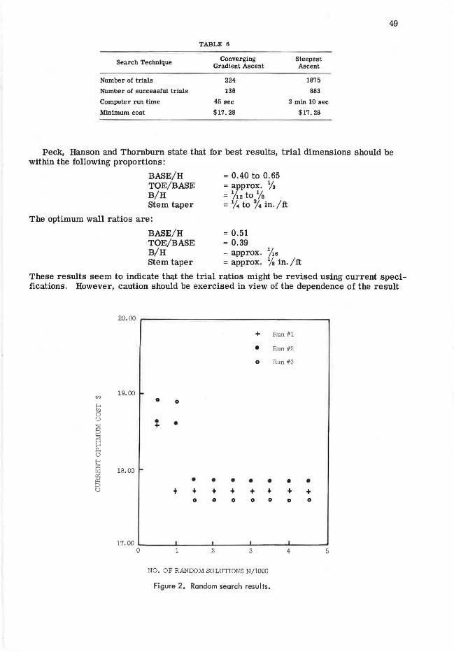
TABLE 6

Search Technique Converging Steepest Gradient Ascent Ascent

Number of trials 224 1875

Number of successful trials 138 883

Computer run time 45 sec 2 min 10 sec

Minimum cost $17. 28 $17. 28

Peck, Hanson and Thornburn state that for best results, trial dimensions should be within the following proportions:

BASE/H TOE/BASE B/H Stem taper

The optimum wall ratios are:

BASE/H TOE/BASE B/H Stem taper

= 0.40 to 0.65 = approx. 1/s = ½2 to 1/a =¼to¾ in./ft

= 0.51 = 0.39 = approx. 1

/ 16

= approx. ¼ in. /ft

These results seem to indicate that the trial ratios might be revised using current speci­fications. However, caution should be exercised in view of the dependence of the result

"" [--,

"' 0 ,_)

s ~ 0. 0 [--, z ril

~ u

20.00

+ Run 411

• Run 412

0 Run a//3

19.00 ,-0 0

• + •

18. 00 -

• • • • • • • + + + + + + + +

0 0 0 0 0 0 0

17.00 _ ___ ....._, __ __. • .__ ___ ,,.__ _ __ ....._, _ _ _

0 2 3 4

NO. OF RANDOM SOLUTIONS N/1000

Figure 2. Random search results.

5

50

on the unit costs of the materials. The computer run time on a UNIV AC 1107 at the University of Notre Dame where the authors conducted the study for the exhaustive search was 25 min and 17 sec.

The results of the converging gradient ascent and steepest ascent search are com­pared in Table 6.

It should be remembered when examining these results that the relative efficiency is quite dependent on the proximity of the starting point to the optimum. In addition, the rapid convergence of the geometric techniques is quite dependent on the nature of the objective function being examined.

The results of three successive runs of 5000 trials each, using the random search approach are shown in Figure 2. All three runs yielded a solution with a cost within 5 percent of the optimum cost after 2000 trials. It should be noted that proximity to the optimum based on cost is not synonymous with the best fraction f in Table 4 because of the nonlinear distribution of number of walls in a particular price bracket. Based on a eomputation rate of approximately 800 trials per minute, t he 2000 trial search was accomplished in approximately 2½ minutes. It is true that the unique optimum was not obtained in this case; however, the ease of application and flexibility tend to balance the limitations .

CONCLUSIONS

In any optimization problem, the designer must balance the following factors:

1. Anticipated savings in construction costs resulting from an optimization over a conventional design;

2. Cost of computer running time; and 3. Cost of formulating the optimizing algorithm which is of course related to its

sophistication.

With regard to the retaining wall example, it has been shown that all three optimi­zation techniques involved computer r unning times of ½o hr or less. At existing com­puter rates this becomes almost a trivial a mount.

The cost of formulating and pexfectin~ the computer pr ogram is less easily quanti­fied. It is a function of the complexity of the technique and the talent of the program­mer. The search techniques employed in this investigation are quite general and yet do not require any undue mathematical prowess. Also, the burden of program formu­lation will probably be considerably eased in the near future as general purpose opti­mization programs become available .

The economy of construction costs must of course be judged on an individual basis; however, in view of the previous discussion the benefits of optimization would not have to be large to justify the effort .

At t he r isk of possibly stating the obvious, there would appear to be a class of rela­tively small, common civil engineering design problems that can be optimized on an economically justifiable basis in a relatively straightforward manner in conjunction with digital computation.

REFERENCES

1. Dantzig, G. B . P rogramming in a Linear Str ucture. Comptroller, USAF, Washington, D. C. , Feb. 1948.

2. Hadley, G. Nonlinear and Dynamic Pr ogra mming. Addison-Wesley, rn1,4 . 3. Kuhn, H. W., and Tucker, A. W. Nonlinear Prog1·amming. Proceedings of the

Second Berkeley Symposium on Mathematical Statistics and Probability, Berkeley, University of California Press, pp. 481-492, 1950.

4. Arrow, K. J., Hurwicz, L., and Uzawa, H. Studies in Linear and Non Linear Programming. Stanford University Press, 1958.

5. Wadsworth, M. A. Sloping Surcharge Retaining Wall Design. 2nd. ASCE Conference on Electronic Computation, Sept. 1960.

6. Peck, R. B., Hanson, W. E., and Thornburn, H. Foundation Engineering. John Wiley & Sons, Inc., 1953.

51

7. Building Code Requirements for Reinforced Concrete (ACI 318-63). Detroit: American Concrete Institute, 1963.

8. Materials Prices-Monthly Market Quotation by ENR Field Reporters. Engineering News-Record, Vol. 178, No. 1, p. 46, Jan. 5, 1967; Vol. 178, No. 2, p. 54, Jan. 12, 1967.

9. Wilde, D. J., Optimum Searching Methods. Prentice Hall, Inc., 1964. 10. Brooks, S. H. A Discussion of Random Methods for Maximum. Operations

Research, Vol. 6., No. 2, p. 244-251., March 1958. 11. Mathematical Optimization Techniques. Computers in Engineering Design

Education. University of Michigan, Vol. 1, p. 42-82, 1966. 12. Hicks, C. R., Fundamental Concepts in the Design of Experiments. Holt,

Rinehart and Winston, 1964.

Discussion G. G. GOBLE, Associate Professor, Case Western Reserve University-This paper gives an interesting application of mathematical programming in civil engineering de­sign. Since a substantial amount of work has been done in applying these methods in structural design, a listing of a few references may be useful to the reader. References (13) through (16) discuss the practical application of optimization in structural design. fureferences;-(17)and (18) the use of linear programming is discussed. NonlineaT pro­gramming has been applied in references (19), (20) and (21) while in reference (22), the structural design problem is converted intoan unconstrained minimization problem. This very brief list is by no means complete, but provides a review of the development of the field. In some of the references highly developed search techniques were used.

The writer agrees enthusiastically with the conclusion that optimizing techniques are ready for routine application in civil engineering design. Perhaps, the greatest impact will come from the freeing of the designer from many tedious design computations so that his effort can be spent on more creative tasks.

References

13 , Razani, R., and Goble, G. Optimum Design of Constant Depth Plate Girders. Jour. of Struct. Div. ASCE, Vol. 92, No. ST2, April 1966.

14. Goble, G., and DeSantis, P. Optimum Design of Composite Girders with Mixed Steel Strengths. Jour. of Struct. Div. ASCE, Vol. 92, No. ST6, April 1966.

15. Goble, G. Structural Synthesis in Cost Oriented Structural Design. Building Research, March-April 1966.

16. Brown, D. and Ang, A. Structural Optimization by Nonlinear Programming. Jour. of Struct. Div. ASCE, Vol. 92, No. ST6, Dec. 1966.

17. Reinschmidt, K., Cornell, C., and Brotchie, J. Iterative Design and Structural Optimization. Jour. of Struct. Div. ASCE, Vol. 92, No. ST6, Dec. 1966.

18. Moses, F. Optimum Structural Design Using Linear Programming. Jour. of Struct. Div. ASCE, Vol. 90, No. ST6, Dec. 1964.

19. Schmit, L A. Structural Design by Systematic Synthesis. Proc. 2nd National Conference on Electronic Computation, Struct. Div. ASCE, Sept. 1960.

20. Schmit, L. A., and Kicher, T. P. Synthesis of Material and Configuration Selection. Jour. of Struct. Div. ASCE, Vol. 88, No. ST3, June 1962.

21 Schmit, L. A., and Mallett, R. H. Structural Synthesis and the Design Parameter Hierarchy. Jour . Struct. Div. ASCE, Vol. 89, No. ST4, Aug. 1963.

22. Schmit, L. A., and Fox, R. L. An Integrated Approach to Structural Synthesis and Analysis. AIAA Jour. Vol. 3, No 6, June 1965.