Retail credit stress testing using a discrete hazard model ... · PDF filespecified by the...
33
Credit card stress testing using a dynamic model with macroeconomic factors Bellotti & Crook Page 1 of 33 Retail credit stress testing using a discrete hazard model with macroeconomic factors 4 June 2013 Keywords: Credit Scoring, Stress Testing, Banking, Finance. Abstract Retail credit models are implemented using discrete survival analysis, enabling macroeconomic conditions to be included as time-varying covariates. In consequence, these models can be used to estimate changes in probability of default given downturn economic scenarios. Compared to traditional models we offer improved methodologies for scenario generation and for the use of them to predict default rates. Monte Carlo simulation is used to generate a distribution of estimated default rates from which Value at Risk and Expected Shortfall are computed as a means of stress testing. Several macroeconomic variables are considered and in particular factor analysis is employed to model the structure between these variables. Two large UK data sets are used to test this approach, resulting in plausible dynamic models and stress test outcomes.
Transcript of Retail credit stress testing using a discrete hazard model ... · PDF filespecified by the...
Credit card stress testing using a dynamic model with macroeconomic factors Bellotti & Crook
Page 1 of 33
Retail credit stress testing using a discrete hazard model
with macroeconomic factors
4 June 2013
Keywords: Credit Scoring, Stress Testing, Banking, Finance.
Abstract
Retail credit models are implemented using discrete survival analysis, enabling
macroeconomic conditions to be included as time-varying covariates. In consequence, these
models can be used to estimate changes in probability of default given downturn economic
scenarios. Compared to traditional models we offer improved methodologies for scenario
generation and for the use of them to predict default rates. Monte Carlo simulation is used to
generate a distribution of estimated default rates from which Value at Risk and Expected
Shortfall are computed as a means of stress testing. Several macroeconomic variables are
considered and in particular factor analysis is employed to model the structure between these
variables. Two large UK data sets are used to test this approach, resulting in plausible
dynamic models and stress test outcomes.
Credit card stress testing using a dynamic model with macroeconomic factors Bellotti & Crook
Page 2 of 33
1. Introduction
Stress testing has become increasingly important in evaluating the riskiness of bank loan
portfolios and they are recognised as a key tool in helping financial institutions make
business strategy, risk management and capital planning decisions (FSA 2008). They allow
us to ask what level of losses we can expect given worst case scenarios when taking a number
of risk factors into account. Stress tests should take into consideration unexpected but also
plausible events from which unexpected losses can be computed. In turn regulatory and
economic capital can be computed as required by the Basel II Accord (BCBS 2005). Usual
practice is to develop stress scenarios outside the context of a risk model and to determine
their effects using a valuation model which goes directly from the macroeconomic values
specified by the stress scenario to the impact on portfolio value independently of any risk
parameters of the portfolio. This has two disadvantages. First the generation of these
scenarios involves a subjective judgement, the scenarios have no formal probabilities
associated with them. Indeed regulators now publish the economic conditions that they wish
banks to use to simulate portfolio default rates (FSA (2013)). Second, the scenarios are
divorced from the usual risk metrics used by the banks (Berkowitz 2000). We follow
Berkowitz (2000) who suggests integrating stress tests into the risk model to address these
problems. An alternative definition of a stress test, and the one used here, is to estimate an
extreme quantile of a loss distribution where the distribution is computed using simulated
values of macroeconomic variables from a distribution covering many decades.
Most models of default for retail credit are either point in time (PIT) or through the cycle
(TTC).Neither of these models are able to give good predictions of default rate (DR) on a
portfolio at arbitrary times through the business cycle since in the first case, a PIT model will
reflect the default rates that existed in the context of the macroeconomic conditions that held
Credit card stress testing using a dynamic model with macroeconomic factors Bellotti & Crook
Page 3 of 33
at the particular point in the business cycle when the model was developed. Of course, in
practice the model may be periodically recalibrated, but such recalibration may not be
forward looking nor functionally dependent on macroeconomic variables. In the second case,
a TTC model will reflect average conditions. We consider a form of dynamic model of
default that includes macroeconomic conditions and therefore allows different estimates of
DR for different economic conditions. This model can be used to consider losses during
downturn periods and forms the basis of a principled approach to stress testing a portfolio.
Rösch and Scheule (2008) present a general stress testing approach based on an asset
correlation model that includes macroeconomic factors and show it can be used to estimate
stressed loss rates, given severe economic scenarios. Bellotti and Crook (2009) use a Cox
Proportional Hazards survival model of time to default. This model has the advantage that
macroeconomic time series data can be included in a principled way into the model as time
varying covariates. They show that the inclusion of macroeconomic variables such as bank
interest rates and earnings was significant and had the expected effect: that is, an increase in
interest rates tends to raise risk of default whilst a rise in earnings tends to lower risk of
default. Bellotti and Crook (2011) estimate discrete time survival models with
macroeconomic conditions for a large credit card portfolio demonstrating how this type of
model can be used to perform a stress test using a Cholesky decomposition to preserve the
covariance structure between the macroeconomic variables. Discrete time survival models
have also been used to model personal bankruptcy (Gross and Souleles 2002) and mortgage
foreclosures (Gerardi et al 2008) with macroeconomic variables, but neither of these papers
show how the models can be used for stress testing. Breeden and Thomas (2008) use a
dynamic model to stress test over several scenarios from past economic crises. They identify
Credit card stress testing using a dynamic model with macroeconomic factors Bellotti & Crook
Page 4 of 33
a number of important macroeconomic indicators of default such as interest rate and GDP but
do not build distributions of estimated DRs.
The use of scenario-based stress tests is now common in the regulation of banks (Hoggarth
and Whitley 2003, FSA 2008, FRS 2009). This approach is based on selecting hypothetical
economic scenarios using judgements supported by prior economic knowledge and
considering plausible developments of the economy. However, this approach is problematic
since it allows a high degree of subjective judgement in the selection process. For example,
recent stress tests of major US banks (FRS 2009) have been criticized since the “more
adverse” conditions it uses are considered too weak. For example, the estimate for adverse
2009 unemployment rate was already exceeded within the year. Baker (2009) estimates that
the US stress test could have under-estimated losses by $120 billion. Clearly, the recent
financial crisis has shown that past stress tests failed, since banks and regulators were left
surprised by levels of losses. Haldane (2009) gives several reasons for this failure. One is
that the banking system has not taken all risk factors into account or has under-estimated their
effect (disaster myopia). A second is that banks never had internal incentives to conduct
stress tests seriously (misaligned incentives). It is clear that further rigour is required in the
stress testing process.
In this paper we consider Monte Carlo simulation for stress testing of consumer credit
portfolios as an alternative to a scenario-based approach. By ‘scenario based approach’ we
mean a set of macroeconomic conditions that are specified by a regulator or an institution’s
own economists. Monte Carlo simulation is a standard approach for stress testing of corporate
credit (Marrison 2002),and the only published work using this method for consumer credit is
by Bellotti & Crook (forthcoming) on which this paper builds.. Monte Carlo simulation
Credit card stress testing using a dynamic model with macroeconomic factors Bellotti & Crook
Page 5 of 33
generates a distribution of estimated loss. It is common to use Value at Risk (VaR) (see
Bluhm et al 2010) to compute extreme loss based on this distribution. However, there is a
distinction between VaR and the requirements of stress testing since VaR captures worst case
in normal circumstances, whereas stress testing attempts to capture losses given unusual
circumstances. There is a connection between the two, but a noticeable difference in value
can emerge when considering non-linear exposures or fat-tail loss distributions (BIS 2005).
For this reason we also report expected shortfall for worse case scenarios.
To generate economic simulations, it is crucially necessary to model the structure of the
macroeconomic data. If one simply simulates the macroeconomic variables independently
when in fact they are correlated would result in inappropriate distributions of default rates. In
this paper we use principal component analysis (PCA) to derive key macroeconomic factors
(MF) which are used in the default model. Factor analysis has been used successfully to
model macroeconomic conditions; for example, the Chicago Fed National Activity Index is a
highly regarded and reliable factor representing the US economy (Federal Reserve Bank of
Chicago 2001). Breitung and Eickmeier (2005) provide a review of the use of static and
dynamic factor models applied to macroeconomic time series. They indicate that results using
factor models are encouraging and give results that are competitive or superior to other
benchmark methods. Gray and Walsh (2008) use PCA in a different type of stress test but do
so only to derive impulse response functions for each of seven different Chilean banks and
do not use a survival model.
Dynamic models of default including macroeconomic conditions are built for two large UK
portfolios of credit cards and used to conduct plausible stress tests using a simulation
Credit card stress testing using a dynamic model with macroeconomic factors Bellotti & Crook
Page 6 of 33
approach. In section 2 we describe our modelling and stress testing methods, in section 3 we
describe our data and give results and in section 4 we discuss our conclusions.
2. Method
We employ a discrete time logistic survival model to estimate a dynamic model of default.
We then use Monte Carlo simulation to generate distributions of estimated DR across an
aggregate of accounts. We discuss each of these techniques in the following subsections.
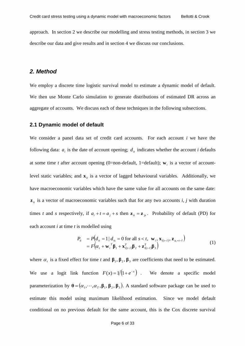
2.1 Dynamic model of default
We consider a panel data set of credit card accounts. For each account i we have the
following data: ia is the date of account opening; itd indicates whether the account i defaults
at some time t after account opening (0=non-default, 1=default); iw is a vector of account-
level static variables; and itx is a vector of lagged behavioural variables. Additionally, we
have macroeconomic variables which have the same value for all accounts on the same date:
itz is a vector of macroeconomic variables such that for any two accounts i, j with duration
times t and s respectively, if sata ji then jsit zz . Probability of default (PD) for
each account i at time t is modelled using
321
,,,allfor0|1
βzβxβw
zxwT
lti
T
lti
T
it
ltaltiiisitit
F
tsddPPi
(1)
where t is a fixed effect for time t and 321 ,, βββ are coefficients that need to be estimated.
We use a logit link function xexF 11)( . We denote a specific model
parameterization by 3211 ,,,,, βββθ T . A standard software package can be used to
estimate this model using maximum likelihood estimation. Since we model default
conditional on no previous default for the same account, this is the Cox discrete survival
Credit card stress testing using a dynamic model with macroeconomic factors Bellotti & Crook
Page 7 of 33
model and the series of fixed effects t form a baseline hazard function. It follows from this
conditionality that dependency of observations within each account is not a problem since
probabilities of events factor out (see Allison 1995, chapter 7).
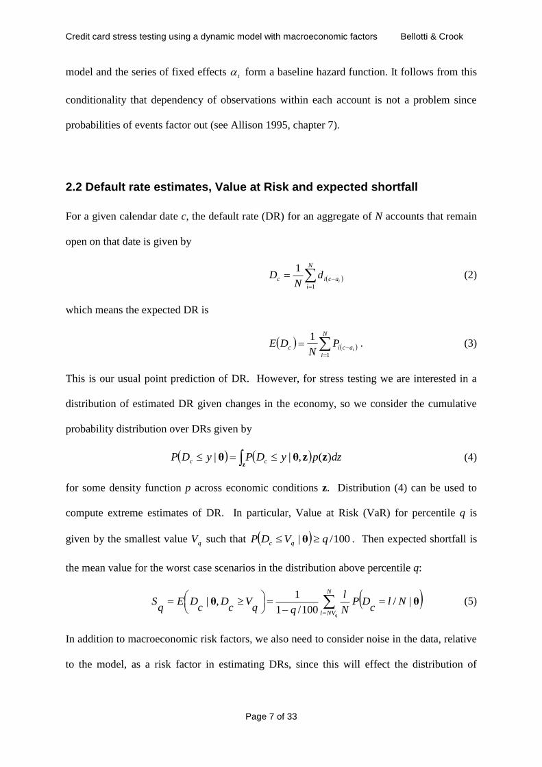
2.2 Default rate estimates, Value at Risk and expected shortfall
For a given calendar date c, the default rate (DR) for an aggregate of N accounts that remain
open on that date is given by
N
i
acic id
ND
1
1 (2)
which means the expected DR is
N
i
acic iP
NDE
1
1. (3)
This is our usual point prediction of DR. However, for stress testing we are interested in a
distribution of estimated DR given changes in the economy, so we consider the cumulative
probability distribution over DRs given by
z
zzθθ dzpyDPyDP cc )(,|| (4)
for some density function p across economic conditions z. Distribution (4) can be used to
compute extreme estimates of DR. In particular, Value at Risk (VaR) for percentile q is
given by the smallest value qV such that 100/| qVDP qc θ . Then expected shortfall is
the mean value for the worst case scenarios in the distribution above percentile q:
N
NVl q
Nlc
DPN
l
qqV
cD
cDE
qS θθ |/
100/1
1,| (5)
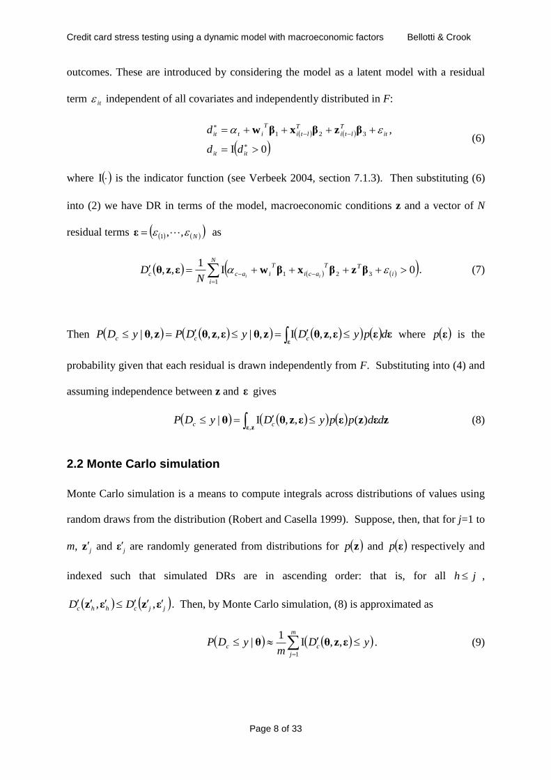
In addition to macroeconomic risk factors, we also need to consider noise in the data, relative
to the model, as a risk factor in estimating DRs, since this will effect the distribution of
Credit card stress testing using a dynamic model with macroeconomic factors Bellotti & Crook
Page 8 of 33
outcomes. These are introduced by considering the model as a latent model with a residual
term it independent of all covariates and independently distributed in F:
0I
,321
itit
it
T
lti
T
lti
T
itit
dd
d βzβxβw (6)
where I is the indicator function (see Verbeek 2004, section 7.1.3). Then substituting (6)
into (2) we have DR in terms of the model, macroeconomic conditions z and a vector of N
residual terms N ,,1 ε as
N
i
i
TT
aci
T
iacc iiND
1
321 0I1
,, βzβxβwεzθ . (7)
Then ε
εεεzθzθεzθzθ dpyDyDPyDP ccc ,,I,|,,,| where εp is the
probability given that each residual is drawn independently from F. Substituting into (4) and
assuming independence between z and ε gives
zε
zεzεεzθθ,
)(,,I| ddppyDyDP cc (8)
2.2 Monte Carlo simulation
Monte Carlo simulation is a means to compute integrals across distributions of values using
random draws from the distribution (Robert and Casella 1999). Suppose, then, that for j=1 to
m, jz and jε are randomly generated from distributions for zp and εp respectively and
indexed such that simulated DRs are in ascending order: that is, for all jh ,
jjchhc DD εzεz ,, . Then, by Monte Carlo simulation, (8) is approximated as
m
j
cc yDm
yDP1
,,I1
| εzθθ . (9)
Credit card stress testing using a dynamic model with macroeconomic factors Bellotti & Crook
Page 9 of 33
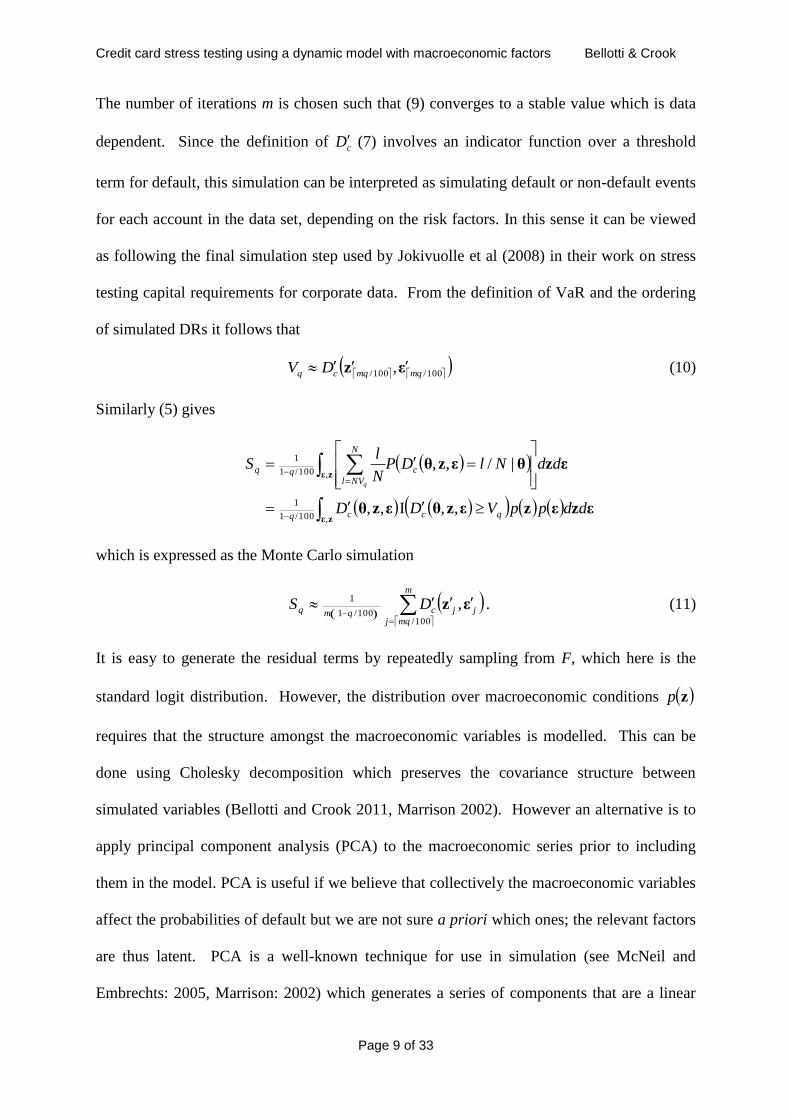
The number of iterations m is chosen such that (9) converges to a stable value which is data
dependent. Since the definition of cD (7) involves an indicator function over a threshold
term for default, this simulation can be interpreted as simulating default or non-default events
for each account in the data set, depending on the risk factors. In this sense it can be viewed
as following the final simulation step used by Jokivuolle et al (2008) in their work on stress
testing capital requirements for corporate data. From the definition of VaR and the ordering
of simulated DRs it follows that
100/100/ , mqmqcq DV εz (10)
Similarly (5) gives
zε
zε
εzεzεzθεzθ
εzθεzθ
,100/1
1
,100/1
1
,,I,,
|/,,
ddppVDD
ddNlDPN
lS
qccq
c
N
NVlqq
q
which is expressed as the Monte Carlo simulation
m
mqj
jjcqmq DS100/
100/1
1,εz . (11)
It is easy to generate the residual terms by repeatedly sampling from F, which here is the
standard logit distribution. However, the distribution over macroeconomic conditions zp
requires that the structure amongst the macroeconomic variables is modelled. This can be
done using Cholesky decomposition which preserves the covariance structure between
simulated variables (Bellotti and Crook 2011, Marrison 2002). However an alternative is to
apply principal component analysis (PCA) to the macroeconomic series prior to including
them in the model. PCA is useful if we believe that collectively the macroeconomic variables
affect the probabilities of default but we are not sure a priori which ones; the relevant factors
are thus latent. PCA is a well-known technique for use in simulation (see McNeil and
Embrechts: 2005, Marrison: 2002) which generates a series of components that are a linear
Credit card stress testing using a dynamic model with macroeconomic factors Bellotti & Crook
Page 10 of 33
combination of a set of random variables such that the first component accounts for as much
of the variability in the data as possible, the second component is orthogonal to the first
whilst accounting for as much of the remainder of the variance, and so on. The problem is
well-posed and is solved by finding eigenvalues and eigenvectors of the matrix of data. For
factor analysis, it is conventional to retain all components with eigenvalues greater than 1.
For details, see Joliffe (2002). Hence, instead of including raw macroeconomic time series,
we use macroeconomic factors (MF) instead. The MFs have the advantage thatthey will not
be correlated with one another, therefore they can be generated independently in the
simulation process. The macroeconomic values are drawn from the historical distribution of
the factors. These are not necessarily normal, so we use the Box-Cox transformation to
model each factor distribution and convert to normal. We do this so that simulations can be
conveniently drawn from a parametric normal distribution fitted to the historic values of the
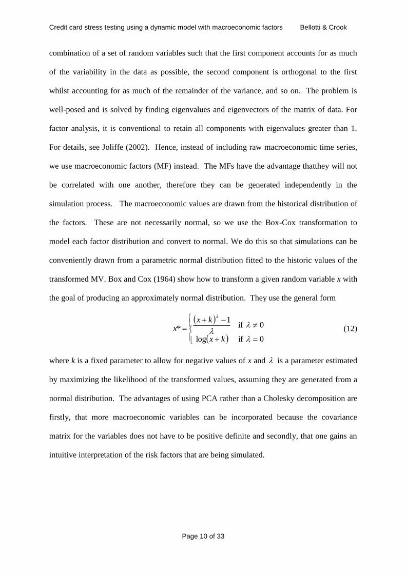
transformed MV. Box and Cox (1964) show how to transform a given random variable x with
the goal of producing an approximately normal distribution. They use the general form
0 iflog
0 if1
*
kx
kxx (12)
where k is a fixed parameter to allow for negative values of x and is a parameter estimated
by maximizing the likelihood of the transformed values, assuming they are generated from a
normal distribution. The advantages of using PCA rather than a Cholesky decomposition are
firstly, that more macroeconomic variables can be incorporated because the covariance
matrix for the variables does not have to be positive definite and secondly, that one gains an
intuitive interpretation of the risk factors that are being simulated.

Credit card stress testing using a dynamic model with macroeconomic factors Bellotti & Crook
Page 11 of 33
2.3 Validation of stress tests
Validation presents a serious challenge to stress tests since, by definition, they are an attempt
to model rare events that have not happened yet. Therefore, it is unlikely we would have test
data that is sufficient to test that the stressed estimates are correct. Consequently, validation
must focus on developing a plausible model structure and on accuracy testing on data we do
have (Breeden 2008).
To compare and contrast using different risk factors, three discrete survival models are built:
No MF: A simple model without any MFs, All MF: A model including all MFs and Selected
MF: A model including only MFs selected using stepwise variable selection. These three
models form the basis of three stress tests using different risk factors. The No MF model is
used for stress tests when only noise in accounts is assumed; the All MF model tests for when
all macroeconomic conditions are included; and the Selected MF model tests for when
macroeconomic conditions are selectively included in the stress test. The Selected MF model
is required since not all MFs are likely to be relevant risk factors and for stress testing, their
inclusion may therefore lead to inaccurate estimates of extreme values. This is particularly
true if any MFs are correlated within the period of the training data which may lead to
multicollinearity and therefore poor estimates for coefficient estimates1. This is unlikely to be
a problem for prediction, when distributions of risk factor values in the forecast data would
be expected to follow those in the training data, but for stress testing, when extreme values of
risk factors are considered, it will more likely have a noticeable effect. By including both the
All MF and Selected MF models, this hypothesis may be tested. Additionally, the coefficient
estimates of the model can themselves be a risk factor, since they are not exact estimates but
have a distribution governed by a covariance matrix which is the outcome of the maximum
1 Although factors will be uncorrelated over the period of PCA, this does not imply they are uncorrelated for any sub-period.
Credit card stress testing using a dynamic model with macroeconomic factors Bellotti & Crook
Page 12 of 33
likelihood procedure. During simulation, these estimates can be adjusted to determine the
effect of estimation uncertainty on the loss distribution. For this reason, we also include a
fourth stress test using the Selected MF model with estimation uncertainty. This will be
the standard model and will be reported simply as the “Selected MF model” in the Results
section.
For accuracy testing, an advantage of the approach we take is that it generates a loss
distribution from which stressed values are derived as VaR or expected shortfall. This means
that although the stressed events themselves cannot easily be tested the underlying loss
distribution can be back-tested against historical data. Most financial institutions should have
sufficient historical data in their retail portfolios to do this. In particular, the loss
distributions can be validated given a time series of observed DRs for a post out-of-sample
data set (Granger and Huang 1997) using a binomial test. To determine if the stress test is
unrealistically conservative we can check if the number of observed defaults that exceed
estimated VaR is likely to occur by chance. For example, if we are considering 99% VaR,
we would expect only 1% of observations to exceed VaR on average and the distribution of
such cases is governed by the binomial distribution which allows us to test the significance of
outcomes (Marrison 2002, chapter 8). The application of the binomial test to this problem is
well-known and forms the basis of the traffic-light validation system used by industry and
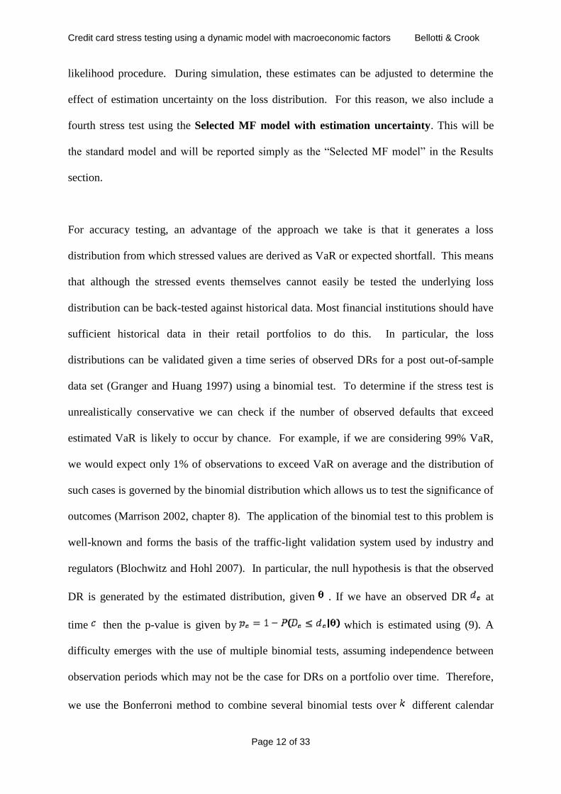
regulators (Blochwitz and Hohl 2007). In particular, the null hypothesis is that the observed
DR is generated by the estimated distribution, given . If we have an observed DR at
time then the p-value is given by which is estimated using (9). A
difficulty emerges with the use of multiple binomial tests, assuming independence between
observation periods which may not be the case for DRs on a portfolio over time. Therefore,
we use the Bonferroni method to combine several binomial tests over different calendar
Credit card stress testing using a dynamic model with macroeconomic factors Bellotti & Crook
Page 13 of 33
times. Regardless of the dependencies between the tests, if we choose a significance level
and one of the null hypotheses is rejected when , then the probability of falsely
rejecting any of the null hypotheses is less than .
3. Experimental Results
3.1 Data
We have two large data sets for two UK credit card products, consisting of over 200,000
accounts each and spanning a period from 1999 to mid-2006. The data consists of (1) data
collected at time of application such as the applicant’s age, income, employment status,
housing status and credit bureau score, (2) account open date and (3) monthly behavioural
data including credit limit, outstanding balance, card usage and payment history: amount paid
and minimum payment required. We define an account as in default when it is recorded as
having failed to make the minimum payments for three consecutive months or more where
the time window over which the missing payments were recorded changes over time as
payments are made2. This definition is typical in the industry and matches the standard
specified by Basel II (BCBS 2005) of 90 days delinquency.
A validation set consisting of one year of data is produced by randomly dividing each product
data set into a training and validation data set in a 2:1 ratio of accounts, then discarding all
records after an observation date of June 2005 from the training data set and keeping only
accounts opened prior to the observation date, but considering only records after the
observation date, for the test set. This procedure ensures (1) there is no selection bias, since
2 For reasons of commercial confidentiality, we cannot reveal descriptive statistics or DRs for these data.
Credit card stress testing using a dynamic model with macroeconomic factors Bellotti & Crook
Page 14 of 33
accounts in the validation data set are selected randomly and independently, (2) the validation
data set is both out-of-sample and post-training data and (3) the validation is realistic in the
sense that only accounts that are known (ie already open) prior to the observation date are
included in the validation set.
Breeden and Thomas (2008) use several macroeconomic variables in their models of default
such as GDP, interest rate, unemployment rate, house price and consumption variables, such
as retail sales, which they argue could impact consumer delinquency. Crook and Bellotti
(2012) also find bank interest rates, earnings, production and house prices significant in
explaining default for different credit card data. We therefore follow with a similar set of
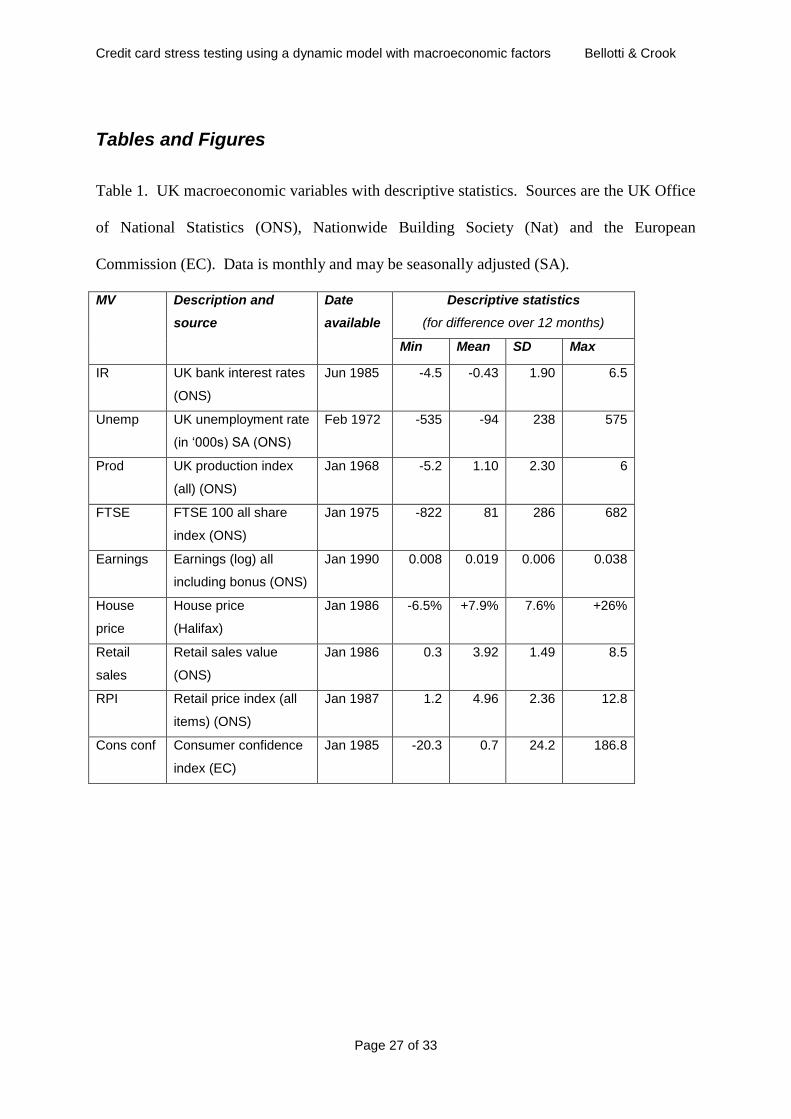
variables described in Table 1. Notice that production index is used instead of GDP since
production index is available monthly in the UK whereas GDP is quarterly. The difference in
the value over 12 months is used for all variables to avoid inadvertently including a time
trend or seasonal variation in the time series. The log value of FTSE, house prices and
earnings are used in the model since these follow an obvious exponential trend. Since both
the behavioural and macroeconomic data is monthly we use discrete monthly time in the
survival model.
TABLE 1 HERE
3.2 Factor analysis
Table 2 shows that PCA applied to the macroeconomic time series from 1986 to June 2006
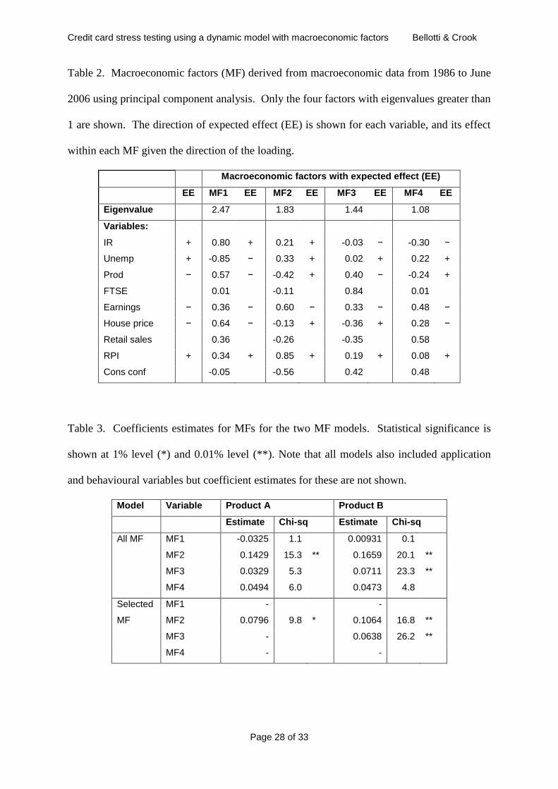
returns 4 factors with an eigenvalue greater than 1. MF1 is loaded on a broad range of
economic variables, but not strongly on FTSE index. MF2 is loaded mainly on consumption
variables: RPI, consumer confidence and earnings. MF3 is driven by the FTSE index,
Credit card stress testing using a dynamic model with macroeconomic factors Bellotti & Crook
Page 15 of 33
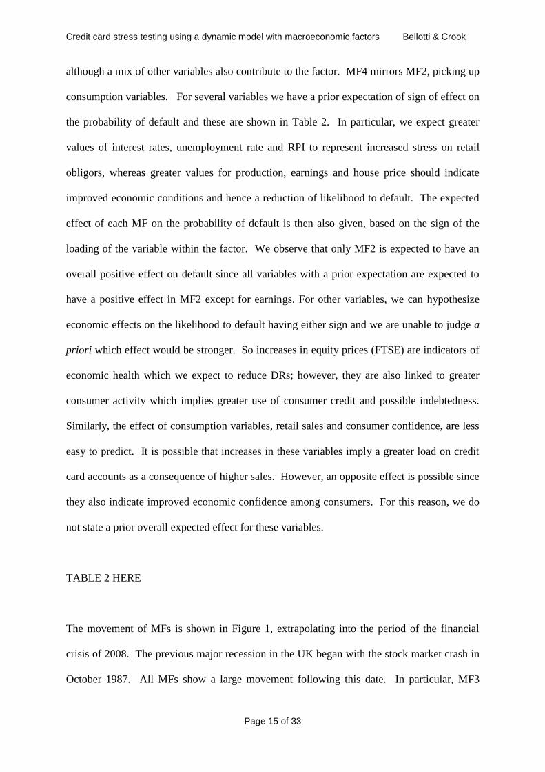
although a mix of other variables also contribute to the factor. MF4 mirrors MF2, picking up
consumption variables. For several variables we have a prior expectation of sign of effect on
the probability of default and these are shown in Table 2. In particular, we expect greater
values of interest rates, unemployment rate and RPI to represent increased stress on retail
obligors, whereas greater values for production, earnings and house price should indicate
improved economic conditions and hence a reduction of likelihood to default. The expected
effect of each MF on the probability of default is then also given, based on the sign of the
loading of the variable within the factor. We observe that only MF2 is expected to have an
overall positive effect on default since all variables with a prior expectation are expected to
have a positive effect in MF2 except for earnings. For other variables, we can hypothesize
economic effects on the likelihood to default having either sign and we are unable to judge a
priori which effect would be stronger. So increases in equity prices (FTSE) are indicators of
economic health which we expect to reduce DRs; however, they are also linked to greater
consumer activity which implies greater use of consumer credit and possible indebtedness.
Similarly, the effect of consumption variables, retail sales and consumer confidence, are less
easy to predict. It is possible that increases in these variables imply a greater load on credit
card accounts as a consequence of higher sales. However, an opposite effect is possible since
they also indicate improved economic confidence among consumers. For this reason, we do
not state a prior overall expected effect for these variables.
TABLE 2 HERE
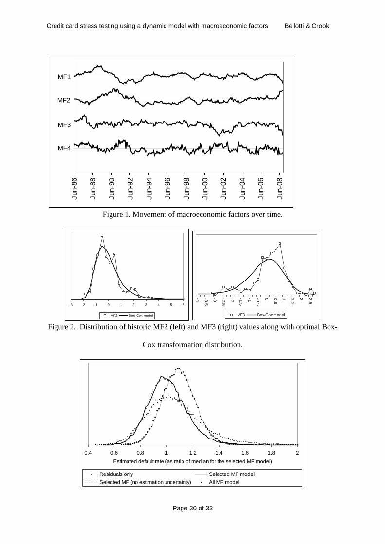
The movement of MFs is shown in Figure 1, extrapolating into the period of the financial
crisis of 2008. The previous major recession in the UK began with the stock market crash in
October 1987. All MFs show a large movement following this date. In particular, MF3
Credit card stress testing using a dynamic model with macroeconomic factors Bellotti & Crook
Page 16 of 33
shows a sharp decline at this time and this is unsurprising given that the main contributor to
MF3 is the FTSE index. However MF2 has the most sustained upward trend for several
years after the beginning of the crisis, indicating strain on consumption after the stock market
crash. Extrapolating into 2008, we see the dramatic effect of the financial crisis during this
period on all MFs. This is evidence that these factors are good indicators of economic stress
and could be used for stress testing.
FIGURE 1 HERE
We apply the Box-Cox transformation to model the factors. Both MF1 and MF3 require no
transformation since their Box-Cox 1 . However, both MF2 and MF3 have long tails and
require a transformation with 1 and 2 respectively as shown in Figure 2.
FIGURE 2 HERE
3.3 Model fit
Along with MFs, the models also include application and behavioural variables and annual
indicator variables for vintage, but these will not be reported in our results since the main
focus of this paper is the inclusion of macroeconomic conditions and stress testing. For
further details about building and assessment of a survival model using application and
macroeconomic variables for retail credit cards, see Bellotti and Crook (2009). Models were
built with behavioural variables lagged by 12 months in order to reduce the possible effect of
endogeneity between behavioural data and default event (eg a rise in account balance and
default may have a common external cause) and to allow for forecasts up to 12 months ahead.
MFs were included with lag 3 months since we anticipate that economic conditions
Credit card stress testing using a dynamic model with macroeconomic factors Bellotti & Crook
Page 17 of 33
contribute to default at the time when payments first begin to be missed. It is possible that
earlier lags could be used but our preliminary experiments indicated that a 3 month lag is
sufficient. For the Selected MF model, a significance level of 1% was chosen selected as a
heuristic for stepwise variable selection. This was sufficient for selection of factors whilst
ensuring highly correlated factors are not included together.
Table 3 shows MF coefficient estimates for models built on training data for each product.
Several factors are statistically significant in the models. In particular, MF2 is a strong driver
in all models and has the direction of effect as expected overall, as shown in Table 2. Figure
2 showed that MF2 was the strongest signal of the effect of the October 1987 stock market
crash, hence its inclusion in the models is promising for stress testing. MF3 is also a driver
for product B although the size of effect is not as large as MF2. There was no overall
expected direction of effect for MF3: as shown in Table 2, three loaded variables have a
positive expected effect aqnd three with a negative expected effect. However FTSE is the
largest contributor to MF3 which implies that the strongest effect of FTSE on likelihood to
default is not as an indicator of economic health but as an indirect indicator of consumer
spending and possible over-indebtedness.
TABLE 3 HERE
The size of effect of MF2 is much larger in the All MF model than the Selected MF model.
This is a consequence of the inclusion of MF4 which has an opposite effect to MF2 over the
period of training (correlation coefficient ) causing multicollinearity between MF2
and MF4 in the model which inflates the coefficient estimate of MF2. As discussed in
Section 2.3, this is not a problem for predictions but may be for stress testing. Variable
Credit card stress testing using a dynamic model with macroeconomic factors Bellotti & Crook
Page 18 of 33
selection resolves this problem by excluding MF4 from the model. There is no significant
correlation between MF2 and MF3 ( ) so the model for product B which includes
both these factors is not affected by multicollinearity.
3.4 Stress test results
Models are built with an observation date of June 2005. Stress tests are then performed for
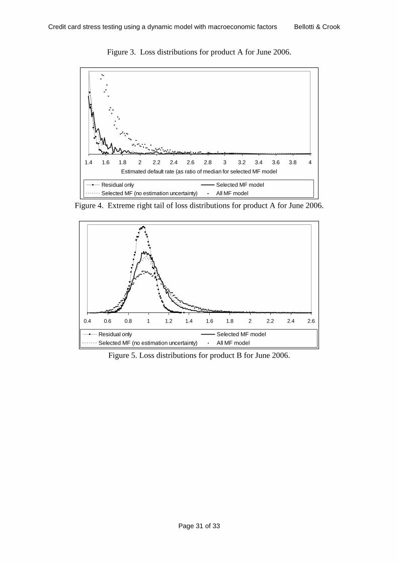
one year ahead, June 2006. Figures 3 to 5 show distributions of estimated DRs following
Monte Carlo simulation on the test set for each product and for stress tests using different risk
factors. We found these distributions converged after 50,000 simulations. For reasons of
commercial confidentiality we cannot report the precise DRs. Instead we report estimated
DR as a ratio of the median estimated DR computed using the Selected MF model. Table 5
shows statistics for each of these distributions in terms of median DR, VaR and expected
shortfall. A level of 99.9% is used since this reflects the standard level recommended for use
in the Basel II Accord.
FIGURE 3 HERE
FIGURE 4 HERE
FIGURE 5 HERE
TABLE 4 HERE
For product A we notice that the shape shown in Figure 3 is approximately the same for both
the No MF and Selected MF models except that the No MF model tends to give higher
estimates. However in Figure 4 the right tail is shown in detail and clearly shows that the
Selected MF model has the longer tail, accounting for the much higher estimates of VaR and
expected shortfall. For product B, the distribution is much broader for the Selected MF
model than the No MF model and, again, the Selected MF model has a long tail, as shown in
Credit card stress testing using a dynamic model with macroeconomic factors Bellotti & Crook
Page 19 of 33
Figure 5. The long tail is typical of loss distributions and we would expect to observe it (BIS
2005). In the case of these experiments, the long tail is a consequence of including MF2 in
the stress test which itself has a long tail (see Figure 2). Comparing the All MF to the
Selected MF models, we find that for both products, the distributions based on the All MF
models are much broader, leading to relatively extreme VaR and unexpected shortfall. This
is a consequence of the inflated coefficient estimates caused by multicollinearity between
MFs, rather than a genuine warning of greater risk. Finally, we note that excluding
estimation uncertainty as a risk factor makes very little difference to the distribution, even at
extremes, and so for practical purposes it can be safely excluded.
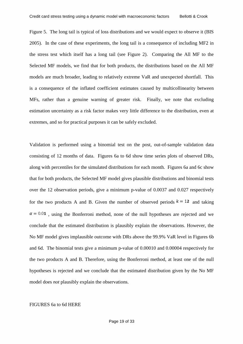
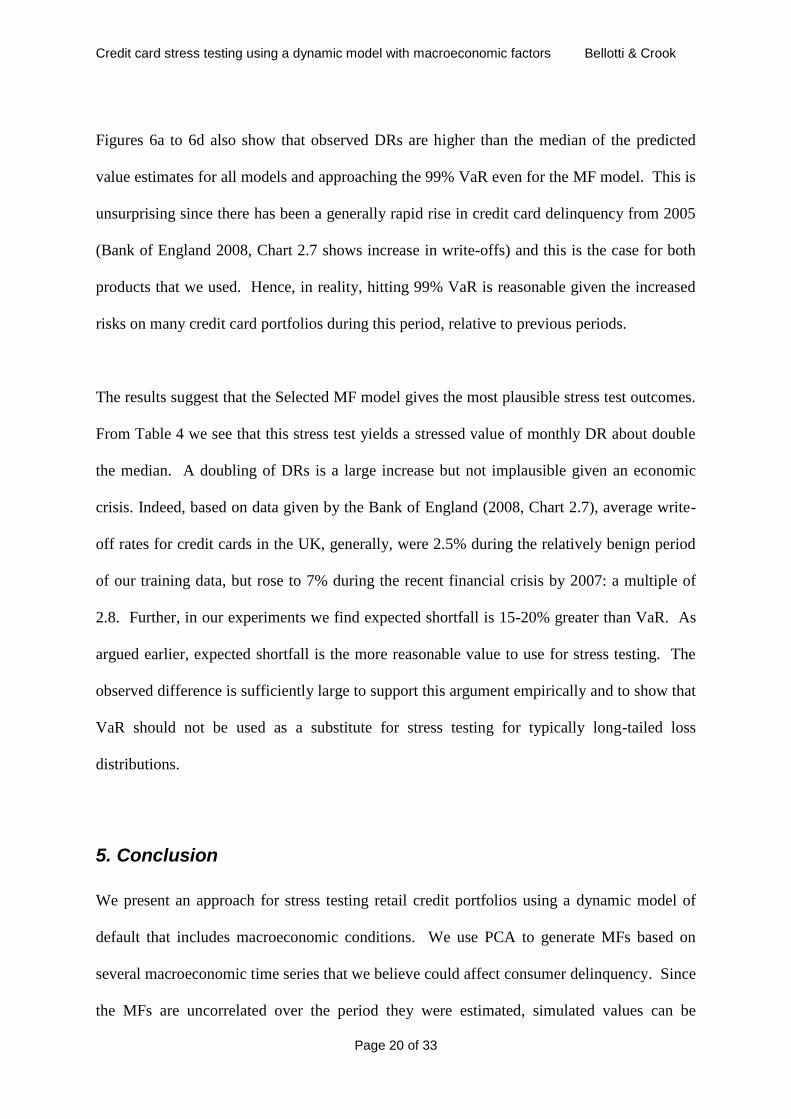
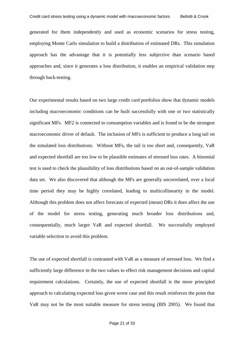
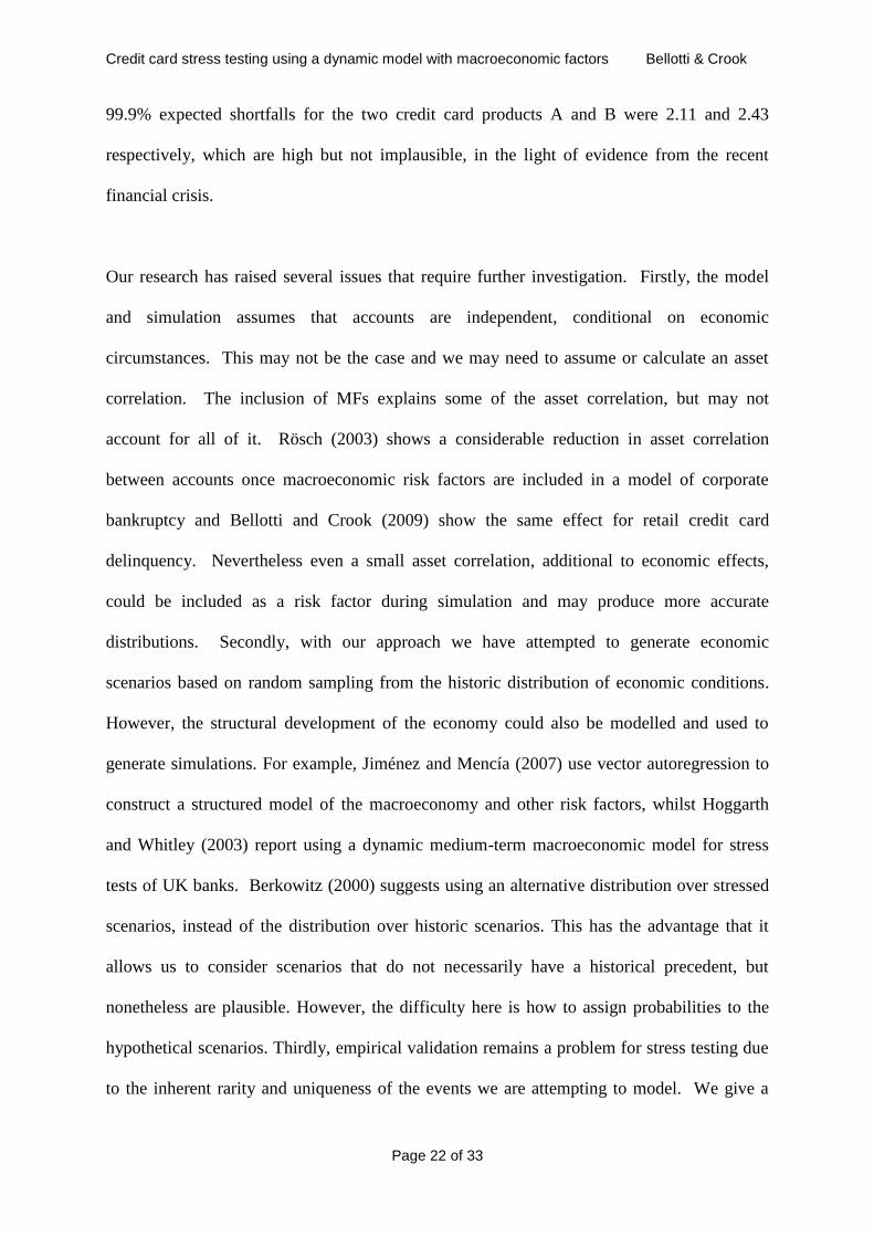
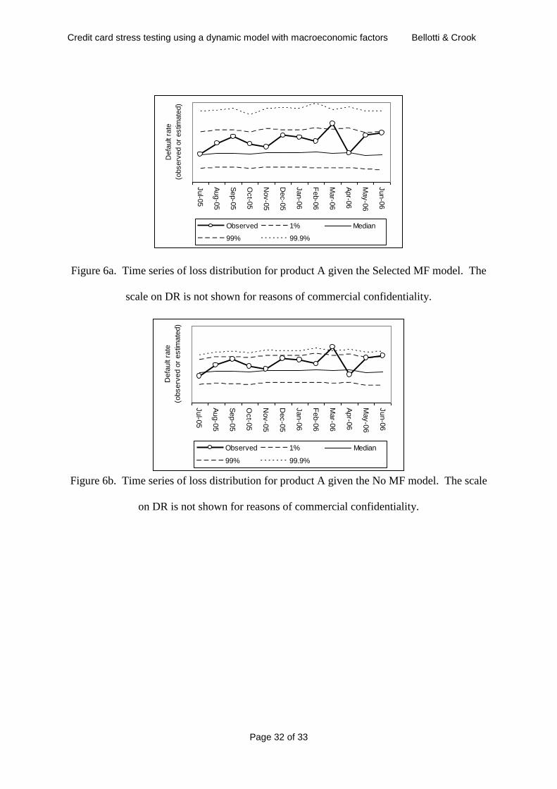
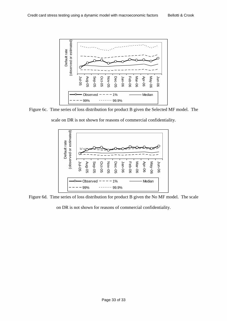
Validation is performed using a binomial test on the post, out-of-sample validation data
consisting of 12 months of data. Figures 6a to 6d show time series plots of observed DRs,
along with percentiles for the simulated distributions for each month. Figures 6a and 6c show
that for both products, the Selected MF model gives plausible distributions and binomial tests
over the 12 observation periods, give a minimum p-value of 0.0037 and 0.027 respectively
for the two products A and B. Given the number of observed periods and taking
, using the Bonferroni method, none of the null hypotheses are rejected and we
conclude that the estimated distribution is plausibly explain the observations. However, the
No MF model gives implausible outcome with DRs above the 99.9% VaR level in Figures 6b
and 6d. The binomial tests give a minimum p-value of 0.00010 and 0.00004 respectively for
the two products A and B. Therefore, using the Bonferroni method, at least one of the null
hypotheses is rejected and we conclude that the estimated distribution given by the No MF
model does not plausibly explain the observations.
FIGURES 6a to 6d HERE
Credit card stress testing using a dynamic model with macroeconomic factors Bellotti & Crook
Page 20 of 33
Figures 6a to 6d also show that observed DRs are higher than the median of the predicted
value estimates for all models and approaching the 99% VaR even for the MF model. This is
unsurprising since there has been a generally rapid rise in credit card delinquency from 2005
(Bank of England 2008, Chart 2.7 shows increase in write-offs) and this is the case for both
products that we used. Hence, in reality, hitting 99% VaR is reasonable given the increased
risks on many credit card portfolios during this period, relative to previous periods.
The results suggest that the Selected MF model gives the most plausible stress test outcomes.
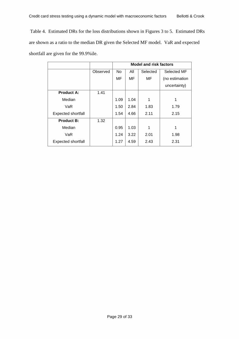
From Table 4 we see that this stress test yields a stressed value of monthly DR about double
the median. A doubling of DRs is a large increase but not implausible given an economic
crisis. Indeed, based on data given by the Bank of England (2008, Chart 2.7), average write-
off rates for credit cards in the UK, generally, were 2.5% during the relatively benign period
of our training data, but rose to 7% during the recent financial crisis by 2007: a multiple of
2.8. Further, in our experiments we find expected shortfall is 15-20% greater than VaR. As
argued earlier, expected shortfall is the more reasonable value to use for stress testing. The
observed difference is sufficiently large to support this argument empirically and to show that
VaR should not be used as a substitute for stress testing for typically long-tailed loss
distributions.
5. Conclusion
We present an approach for stress testing retail credit portfolios using a dynamic model of
default that includes macroeconomic conditions. We use PCA to generate MFs based on
several macroeconomic time series that we believe could affect consumer delinquency. Since
the MFs are uncorrelated over the period they were estimated, simulated values can be
Credit card stress testing using a dynamic model with macroeconomic factors Bellotti & Crook
Page 21 of 33
generated for them independently and used as economic scenarios for stress testing,
employing Monte Carlo simulation to build a distribution of estimated DRs. This simulation
approach has the advantage that it is potentially less subjective than scenario based
approaches and, since it generates a loss distribution, it enables an empirical validation step
through back-testing.
Our experimental results based on two large credit card portfolios show that dynamic models
including macroeconomic conditions can be built successfully with one or two statistically
significant MFs. MF2 is connected to consumption variables and is found to be the strongest
macroeconomic driver of default. The inclusion of MFs is sufficient to produce a long tail on
the simulated loss distributions. Without MFs, the tail is too short and, consequently, VaR
and expected shortfall are too low to be plausible estimates of stressed loss rates. A binomial
test is used to check the plausibility of loss distributions based on an out-of-sample validation
data set. We also discovered that although the MFs are generally uncorrelated, over a local
time period they may be highly correlated, leading to multicollinearity in the model.
Although this problem does not affect forecasts of expected (mean) DRs it does affect the use
of the model for stress testing, generating much broader loss distributions and,
consequentially, much larger VaR and expected shortfall. We successfully employed
variable selection to avoid this problem.
The use of expected shortfall is contrasted with VaR as a measure of stressed loss. We find a
sufficiently large difference in the two values to effect risk management decisions and capital
requirement calculations. Certainly, the use of expected shortfall is the more principled
approach to calculating expected loss given worst case and this result reinforces the point that
VaR may not be the most suitable measure for stress testing (BIS 2005). We found that
Credit card stress testing using a dynamic model with macroeconomic factors Bellotti & Crook
Page 22 of 33
99.9% expected shortfalls for the two credit card products A and B were 2.11 and 2.43
respectively, which are high but not implausible, in the light of evidence from the recent
financial crisis.
Our research has raised several issues that require further investigation. Firstly, the model
and simulation assumes that accounts are independent, conditional on economic
circumstances. This may not be the case and we may need to assume or calculate an asset
correlation. The inclusion of MFs explains some of the asset correlation, but may not
account for all of it. Rösch (2003) shows a considerable reduction in asset correlation
between accounts once macroeconomic risk factors are included in a model of corporate
bankruptcy and Bellotti and Crook (2009) show the same effect for retail credit card
delinquency. Nevertheless even a small asset correlation, additional to economic effects,
could be included as a risk factor during simulation and may produce more accurate
distributions. Secondly, with our approach we have attempted to generate economic
scenarios based on random sampling from the historic distribution of economic conditions.
However, the structural development of the economy could also be modelled and used to
generate simulations. For example, Jiménez and Mencía (2007) use vector autoregression to
construct a structured model of the macroeconomy and other risk factors, whilst Hoggarth
and Whitley (2003) report using a dynamic medium-term macroeconomic model for stress
tests of UK banks. Berkowitz (2000) suggests using an alternative distribution over stressed
scenarios, instead of the distribution over historic scenarios. This has the advantage that it
allows us to consider scenarios that do not necessarily have a historical precedent, but
nonetheless are plausible. However, the difficulty here is how to assign probabilities to the
hypothetical scenarios. Thirdly, empirical validation remains a problem for stress testing due
to the inherent rarity and uniqueness of the events we are attempting to model. We give a
Credit card stress testing using a dynamic model with macroeconomic factors Bellotti & Crook
Page 23 of 33
binomial test approach on the underlying loss distributions. However, it is primarily a test to
reject loss distributions that are clearly implausible. The binomial test still cannot test the
validity of extreme value estimates (above the 99th percentile) and therefore cannot be used to
positively validate the plausibility of VaR and expected shortfall. Further development of
empirical tests of extreme values would be valuable. For example, Wong (2009) suggests an
alternative approach using a size of tail loss statistic instead of a binomial test and finds this
has more statistical power. Nevertheless, a simple binomial test gives plausibility to the
overall loss distribution, providing further confidence in their use for stress tests.
Credit card stress testing using a dynamic model with macroeconomic factors Bellotti & Crook
Page 24 of 33
References
Allison PD (1995). Survival analysis using SAS. SAS Press.
Basel Committee on Banking Supervision BCBS (2005). Basel II: International
Convergence of Capital Measurement and Capital Standards at www.bis.org/publ/bcbsca.htm
BIS : Bank for International Settlements (2005). Stress testing at major financial institutions:
survey results and practice. Working report from Committee on the Global Financial
System.
Bank of England (2008). Financial Stability Review, April 2008.
Baker D (2009). Background on the Stress Tests: Anyone Got an Extra $120 Billion? Beat
the Press Blog, The American Prospect, 8 May 2009.
Bellotti, T. and Crook, J. (2011) Forecasting and Stress testing Credit Card Default using
Dynamic Models. International Journal of Forecasting (forthcoming).
Bellotti T and Crook J (2009). Credit scoring with macroeconomic variables using survival
analysis. The Journal of the Operational Research Society (2009 ) 60, 1699-1707.
Berkowitz J (2000). A coherent framework for stress testing, The Journal of Risk, Vol 2, No
2, Winter 1999/2000
Blochwitz S and Hohl S (2007). Validation of Banks’ Internal rating Systems – a
Supervisory Perspective in The Basel Handbook 2nd edition ed. Ong M (Risk Books).
Bluhm, C, Overbeck, L, and Wagner, C (2010) An Introduction to Credit Risk Modelling.
Chapman & hall/CRC.
Box GEP and Cox DR (1964). An analysis of transformations. Journal of the Royal
Statistical Society, Series B 26: pp211–246
Breitung, and Eickmeier, S (2005). Dynamic Factor Models. Deutsche Bundesbank,
Discussion Paper, Series 1: Economic Studies, No 38/2005.
Breeden J (2008). Survey of Retail Loan Portfolio Stress Testing. From Stress Testing for
Financial Institutions; ed. Rösch and Scheule (Riskbooks) pp. 129-157.
Breeden J and Thomas L (2008). A common framework for stress testing retail portfolios
across countries. The Journal of Risk Model Validation 2(3), 11-44.
Crook J and Bellotti T (2012) Asset correlations for credit card defaults. Applied Financial
Economics 2012, 22, 87-95.
Federal Reserve Bank of Chicago (2001). CFNAI Background Release, working paper.
Credit card stress testing using a dynamic model with macroeconomic factors Bellotti & Crook
Page 25 of 33
FRS: Board of Governors of the Federal Reserve System (2009). The supervisory capital
assessment program: overview of results. White paper, May 7 2009,FRS.
FSA(2013) :http://www.fsa.gov.uk/about/what/international/stress_testing/firm_s/pillar_2_str
ess_testing/supervisory_recommended_scenarios
FSA (2008): Financial Services Authority UK (2008). Stress and scenario testing.
Consultation paper 08/24.
Gerardi K, Shapiro AH, Willen PS (2008). Subprime outcomes: risky mortgages,
homeownership experiences, and foreclosures. Working paper 07-15 Federal Reserve Bank
of Boston.
Granger CWJ and Huang LL (1997). Evaluation of panel data models: some suggestions
from time series. Discussion paper 97-10, Department of Economics, University of
Caliafornia, San Diego.
Gray, D. and Walsh, J.P. (2008) Factor Model for Stress-testing with a Contingent Claims
Model fof the Chilean Banking System. IMF Working paper, WP/08/89.
Gross DB and Souleles NS (2002). An empirical analysis of personal bankruptcy and
delinquency. The Review of Financial Studies Vol 15, no 1, pp319-347.
Haldane AG (2009), Why the banks failed the stress test, basis of a speech given at the
Marcus-Evans Conference on Stress-Testing, 13 Febuary 2009, Bank of England.
Hoggarth G and Whitley J (2003). Assessing the strength of UK banks through
macroeconomic stress tests. Financial Stability Review, June 2003, Bank of England.
Jiménez G and Mencía (2007). Modelling the distribution of credit losses with observable
and latent factors. Banco de Espana Research Paper.
Joliffe IT (2002). Principal component analysis. (2nd ed, Springer).
Jokivuolle E, Virolainen K and Vähämaa (2008). Macro-model-based stress testing of Basel
II capital requirements. Bank of Finland research discussion papers 17/2008.
Marrison C (2002). Fundamentals of Risk Measurement (McGraw-Hill NY).
Mc Neil, A. and Embrechts, P. (2005). Quantitative Risk Management, Princeton University
Press.
Robert CP and Casella G (1999). Monte Carlo Statistical Methods (Springer).
Rösch D (2003). Correlations and business cycles of credit risk: evidence from bankruptcies
in Germany. Swiss Society for Financial Market Research vol 17(3) pp 309-331.
Credit card stress testing using a dynamic model with macroeconomic factors Bellotti & Crook
Page 26 of 33
Rösch D and Scheule H (2008). Integrating Stress-Testing Frameworks. From Stress Testing
for Financial Institutions; ed. Rösch and Scheule (Riskbooks) pp. 3-15.
Verbeek (2004). A Guide to Modern Econometrics (2nd ed, Wiley).
Wong, Woon K (2009), Backtesting Value-at-Risk based on tail losses, Journal of Empirical
Finance, doi: 10.1016/j.jempfin.2009.11.004
Credit card stress testing using a dynamic model with macroeconomic factors Bellotti & Crook
Page 27 of 33
Tables and Figures
Table 1. UK macroeconomic variables with descriptive statistics. Sources are the UK Office
of National Statistics (ONS), Nationwide Building Society (Nat) and the European
Commission (EC). Data is monthly and may be seasonally adjusted (SA).
MV Description and
source
Date
available
Descriptive statistics
(for difference over 12 months)
Min Mean SD Max
IR UK bank interest rates
(ONS)
Jun 1985 -4.5 -0.43 1.90 6.5
Unemp UK unemployment rate
(in ‘000s) SA (ONS)
Feb 1972 -535 -94 238 575
Prod UK production index
(all) (ONS)
Jan 1968 -5.2 1.10 2.30 6
FTSE FTSE 100 all share
index (ONS)
Jan 1975 -822 81 286 682
Earnings Earnings (log) all
including bonus (ONS)
Jan 1990 0.008 0.019 0.006 0.038
House
price
House price
(Halifax)
Jan 1986 -6.5% +7.9% 7.6% +26%
Retail
sales
Retail sales value
(ONS)
Jan 1986 0.3 3.92 1.49 8.5
RPI Retail price index (all
items) (ONS)
Jan 1987 1.2 4.96 2.36 12.8
Cons conf Consumer confidence
index (EC)
Jan 1985 -20.3 0.7 24.2 186.8
Credit card stress testing using a dynamic model with macroeconomic factors Bellotti & Crook
Page 28 of 33
Table 2. Macroeconomic factors (MF) derived from macroeconomic data from 1986 to June
2006 using principal component analysis. Only the four factors with eigenvalues greater than
1 are shown. The direction of expected effect (EE) is shown for each variable, and its effect
within each MF given the direction of the loading.
Macroeconomic factors with expected effect (EE)
EE MF1 EE MF2 EE MF3 EE MF4 EE
Eigenvalue 2.47 1.83 1.44 1.08
Variables:
IR + 0.80 + 0.21 + -0.03 − -0.30 −
Unemp + -0.85 − 0.33 + 0.02 + 0.22 +
Prod − 0.57 − -0.42 + 0.40 − -0.24 +
FTSE 0.01 -0.11 0.84 0.01
Earnings − 0.36 − 0.60 − 0.33 − 0.48 −
House price − 0.64 − -0.13 + -0.36 + 0.28 −
Retail sales 0.36 -0.26 -0.35 0.58
RPI + 0.34 + 0.85 + 0.19 + 0.08 +
Cons conf -0.05 -0.56 0.42 0.48
Table 3. Coefficients estimates for MFs for the two MF models. Statistical significance is
shown at 1% level (*) and 0.01% level (**). Note that all models also included application
and behavioural variables but coefficient estimates for these are not shown.
Model Variable Product A Product B
Estimate Chi-sq Estimate Chi-sq
All MF MF1 -0.0325 1.1 0.00931 0.1
MF2 0.1429 15.3 ** 0.1659 20.1 **
MF3 0.0329 5.3 0.0711 23.3 **
MF4 0.0494 6.0 0.0473 4.8
Selected MF1 - -
MF MF2 0.0796 9.8 * 0.1064 16.8 **
MF3 - 0.0638 26.2 **
MF4 - -
Credit card stress testing using a dynamic model with macroeconomic factors Bellotti & Crook
Page 29 of 33
Table 4. Estimated DRs for the loss distributions shown in Figures 3 to 5. Estimated DRs
are shown as a ratio to the median DR given the Selected MF model. VaR and expected
shortfall are given for the 99.9%ile.
Model and risk factors
Observed No
MF
All
MF
Selected
MF
Selected MF
(no estimation
uncertainty)
Product A: 1.41
Median 1.09 1.04 1 1
VaR 1.50 2.84 1.83 1.79
Expected shortfall 1.54 4.66 2.11 2.15
Product B: 1.32
Median 0.95 1.03 1 1
VaR 1.24 3.22 2.01 1.98
Expected shortfall 1.27 4.59 2.43 2.31
Credit card stress testing using a dynamic model with macroeconomic factors Bellotti & Crook
Page 30 of 33
Jun-8
6
Jun-8
8
Jun-9
0
Jun-9
2
Jun-9
4
Jun-9
6
Jun-9
8
Jun-0
0
Jun-0
2
Jun-0
4
Jun-0
6
Jun-0
8
Figure 1. Movement of macroeconomic factors over time.
-3 -2 -1 0 1 2 3 4 5 6
MF2 Box-Cox model
-4 -3.5
-3 -2.5
-2 -1.5
-1 -0.5
0 0.5
1 1.5
2 2.5
MF3 Box-Cox model
Figure 2. Distribution of historic MF2 (left) and MF3 (right) values along with optimal Box-
Cox transformation distribution.
0.4 0.6 0.8 1 1.2 1.4 1.6 1.8 2
Estimated default rate (as ratio of median for the selected MF model)
Residuals only Selected MF model
Selected MF (no estimation uncertainty) All MF model
MF1
MF2
MF3
MF4
Credit card stress testing using a dynamic model with macroeconomic factors Bellotti & Crook
Page 31 of 33
Figure 3. Loss distributions for product A for June 2006.
1.4 1.6 1.8 2 2.2 2.4 2.6 2.8 3 3.2 3.4 3.6 3.8 4
Estimated default rate (as ratio of median for selected MF model
Residual only Selected MF model
Selected MF (no estimation uncertainty) All MF model
Figure 4. Extreme right tail of loss distributions for product A for June 2006.
0.4 0.6 0.8 1 1.2 1.4 1.6 1.8 2 2.2 2.4 2.6
Residual only Selected MF model
Selected MF (no estimation uncertainty) All MF model
Figure 5. Loss distributions for product B for June 2006.
Credit card stress testing using a dynamic model with macroeconomic factors Bellotti & Crook
Page 32 of 33
Jul-0
5
Aug-0
5
Sep-0
5
Oct-0
5
Nov-0
5
Dec-0
5
Jan-0
6
Feb-0
6
Mar-0
6
Apr-0
6
May-0
6
Jun-0
6D
efa
ult
rate
(observ
ed o
r estim
ate
d)
Observed 1% Median
99% 99.9%
Figure 6a. Time series of loss distribution for product A given the Selected MF model. The
scale on DR is not shown for reasons of commercial confidentiality.
Jul-0
5
Aug-0
5
Sep-0
5
Oct-0
5
Nov-0
5
Dec-0
5
Jan-0
6
Feb-0
6
Mar-0
6
Apr-0
6
May-0
6
Jun-0
6D
efa
ult
rate
(observ
ed o
r estim
ate
d)
Observed 1% Median
99% 99.9%
Figure 6b. Time series of loss distribution for product A given the No MF model. The scale
on DR is not shown for reasons of commercial confidentiality.
Credit card stress testing using a dynamic model with macroeconomic factors Bellotti & Crook
Page 33 of 33
Jul-0
5
Aug-0
5
Sep-0
5
Oct-0
5
Nov-0
5
Dec-0
5
Jan-0
6
Feb-0
6
Mar-0
6
Apr-0
6
May-0
6
Jun-0
6D
efa
ult
rate
(observ
ed o
r estim
ate
d)
Observed 1% Median
99% 99.9%
Figure 6c. Time series of loss distribution for product B given the Selected MF model. The
scale on DR is not shown for reasons of commercial confidentiality.
Jul-0
5
Aug-0
5
Sep-0
5
Oct-0
5
Nov-0
5
Dec-0
5
Jan-0
6
Feb-0
6
Mar-0
6
Apr-0
6
May-0
6
Jun-0
6D
efa
ult r
ate
(observ
ed o
r estim
ate
d)
Observed 1% Median
99% 99.9%
Figure 6d. Time series of loss distribution for product B given the No MF model. The scale
on DR is not shown for reasons of commercial confidentiality.