t

at

Results of a Monte Carlo investigation of thediffuse attenuation coefficient

Brian M. Concannon and Jon P. Davis

There has been a large effort to relate the apparent optical properties of ocean water to the inherent opticalproperties, which are the absorption coefficient a, the scattering coefficient b, and the scattering phasefunction r~u!. The diffuse attenuation coefficient kdiff has most often been considered an apparent opticalproperty. However, kdiff can be considered a quasi-inherent property kdiff9 when defined as a steady-statelight distribution attenuation coefficient. The Honey–Wilson research empirically relates kdiff to a and b.The Honey–Wilson relation most likely applies to a limited range of water types because it does not includedependence on r~u!. A series of Monte Carlo simulations were initiated to calculate kdiff9 in an unstratifiedwater column. The calculations, which reflected open ocean water types, used ranges of the single-scattering albedo v0 and the mean forward-scattering angle um for two analytic phase functions withdifferent shapes. It was found that kdiff9 is nearly independent of the shape of r~u! and can be easilyparameterized in terms of a, b, and um for 0.11 # um # 0.48 rad and 0.5 # v0 # 0.95. kdiff9 is an asymptoticquantity; that is, a steady-state distribution is reached only after many scattering lengths.

OCIS codes: 010.0010, 120.5820.

r

s

afaa

fg

1. Introduction

It is of great interest to measure the inherent opticalproperties that are invariant to changes in the angu-lar distribution of light as opposed to apparent opticalproperties that are dependent on the angular distri-bution of light.1 The inherent water properties areimportant because they are transferable among dif-ferent measuring systems.

A popular in situ measurement is the diffuse at-enuation coefficient kdiff. In simplest terms, kdiff

measures the sunlight intensity at depth by droppingan upward-looking photosensitive device downthrough the water column. The question that arisesis: Can kdiff be related to the inherent optical prop-erties? On the basis of a limited data set, Sorensonet al. proposed the following relation:

kdiff 5 a 1 byn, (1)

where n ' 6.2 Furthermore, it has been stated thatkdiff can be considered a quasi-inherent optical prop-erty.3 It is our belief that Eq. ~1! is not applicable toll water types because it does not take into accounthe phase function.

The authors are with the Aircraft Division, Naval Air WarfareCenter, Code 4556, Unit 6, Building 2185, 22347 Cedar Point Road,Suite 1100, Patuxent River, Maryland 20670-1161. The e-mailaddress for B. Concannon is concannonbm@navair.navy.mil.

Received 30 November 1998; revised manuscript received 5April 1999.

5104 APPLIED OPTICS y Vol. 38, No. 24 y 20 August 1999

To investigate the validity of the Honey–Wilsonelation we initiated a series of simulated kdiff mea-

surements using the Monte Carlo technique. Wedid not consider the wavelength of the light in any ofthe calculations and we considered only an unstrati-fied water column. The variables in the calculationswere the absorption coefficient a, the scattering coef-ficient b, and the phase function r~u!. We used apherical coordinate system where u is the polar an-

gle and the phase function is independent of the az-imuthal angle f. We used two differently shapednalytic phase functions and two measured phaseunctions. Each of the analytic phase functions hadn adjustable parameter, which changed the meanngle um for that phase function.Our approach was to assume that the form of Eq.

~1! was correct, but the by6 term should be byn andthat n would depend on a, b, and r~u! in some way.We determined the steady-state light distribution at-tenuation coefficient kdiff9 for the two artificial phaseunctions with many different mean scattering an-les. For each um we determined kdiff9 for 11 single-

scattering albedos v0 defined as

v0 5 by~a 1 b!. (2)

We also used two measured phase functions that gen-erally bound r~u! for open ocean water, A and PB,4that represent forward to more diffuse scattering,respectively. The data generated with the analyticphase functions fit the following equation with a 2.6%

i

a

T

RMS error, and the data generated with the mea-sured phase functions fit with a 2.9% RMS error:

kdiff9 5 a 1 ~1.43–1.17v0!um b. (3)

2. Details of the Monte Carlo Implementation

The idea behind a Monte Carlo simulation is to followindividual photons for a given amount of time or dis-tance, while keeping track of the photons’ positionand direction. The photons are allowed to be ran-domly scattered or absorbed based on environmentalparameters. At the completion of the simulation thepositions, directions, and distributions of the manyphotons closely resemble real-life situations given theaccuracy of the reproduction of the environmentalparameters. The following is a description of theimplementation of the Monte Carlo simulation forthis body of research.

The initial conditions of each photon were generatedto simulate a sunny day such that a square area of seasurface was illuminated by a collimated, uniformly dis-tributed beam of photons impinging on the water’ssurface at normal incidence. The simulation startedeach photon at the flat surface of the body of water.To maintain the illusion of a large body of water,boundary conditions were set so that if a photon prop-agated out of the original square that it was launchedin, the photon was brought back in on the exact oppo-site side as if it had come from an adjacent square.

Once launched at the surface, the propagation of anindividual photon followed a few basic steps. First apath length L was determined by

L 5 ~21yb!ln t, (4)

where 1yb is the mean free path between scatteringevents and t is a uniformly distributed random num-ber between 0 and 1.5 Next the photon was propa-gated based on its current scattering angle u, rotationangle f, and L.

The probability of survival Ps for a photon travelingdistance L in a medium with absorption coefficient as calculated by

Ps 5 exp~2aL!. (5)

Each photon launched propagates to the terminationdepth and then Ps is calculated for the total pathlength the photon traveled.6 How the total Ps wasused is described in Section 3.

At a scattering event, new u, f, and L were calcu-lated and the photon was propagated based on thatinformation and the photon’s previous direction vector.The rotation angle f was determined by a uniformlydistributed random number between 0 and 2p. Thescattering angles u were selected randomly from a ta-ble that was generated from a forward-scatteringphase function. Backscatter is not important in thepresent study and if used would add yet another vari-able. We therefore chose to use phase functions de-fined only in the forward hemisphere, for u 5 0 to py2rad. The angle table was generated in the followingmanner: ~1! The phase function is normalized such

that the integral of sin~u!r~u! from 0 to py2 rad equalsunity, ~2! the total number of equally probable bins~scattering angles! to be used was chosen arbitrarily,~3! the probability for each bin was the reciprocal of thenumber of bins to be used, ~4! the first bin was chosensuch that the integral of sin~u!r~u! over the first binequaled the bin probability, ~5! the first scattering an-gle was the mean angle of the first bin, ~7! the last twosteps were repeated for all bins, and ~7! the adequacyof the number of bins chosen was verified by samplecalculations using differing numbers of bins in theMonte Carlo simulations.

The Merten–Wells phase function7

r~u! 5 ~CMWu0!y@2p~u02 1 u2!3y2# (6)

nd the Arnush phase function8

r~u! 5 ~CAgy2pu!exp~2gu!, (7)

where CMW and CA are determined by

*0

py2

du sin~u!r~u! 5 1, (8)

were used in the calculations with various values ofu0 and g, respectively, to generate phase functionsthat allowed highly forward to more diffuse scatter-ing. The mean angle of r~u! is calculated as

um 5 *0

py2

du sin~u!r~u!u. (9)

he correctness of the table is confirmed calculating umfrom the generated scattering angle table by summingup the angles in the table and dividing by the numberof elements in the table. In Fig. 1, sin~u!r~u! is plottedversus u for both artificial phase functions to showthat, although their mean angles are the nearly thesame, the variance of the two phase functions differ bya factor of 2. In addition, two measured phase func-tions, A ~um 5 0.25 rad! and PB ~um 5 0.38 rad!, listedin Gordon et al.4 were used. These two phase func-tions, plotted in Fig. 2, were described in Ref. 4 aslikely to be the most and least forward-scattering func-tions occurring in clear ocean water.

Fig. 1. Merten–Wells and Arnush analytic phase functions.

20 August 1999 y Vol. 38, No. 24 y APPLIED OPTICS 5105

ppcantwp

w

Te

pd

ds

m

5

The scattering and propagation were continued un-til the photon passed through a depth plane of interest.The sum of the path lengths Ltotal that the photonropagated along to reach the depth plane and thehoton’s relative position in the depth plane were re-orded for later processing. Other parameters, suchs u and f, could also have been saved but were notecessary for this experiment. The simulation con-inued through many depth planes until the photonas terminated at some predetermined depth. If ahoton’s Ltotal exceeded six times the final depth, the

photon was terminated and considered lost.

3. Data Collection and Processing

At the end of a typical simulation in which 200,000photons were propagated, we had a file containingthe total path length traveled to various depth planesand the position in the plane of each photon. Tosimulate a k-meter measurement, all the photons

ithin a fixed aperture at each depth plane dn wereweighted individually by calculating Ps from Eq. ~5!.

he sum of the weights of the collected photons inach depth plane ¥Ps~dn! was then used to calculate

the decay rate of the sunlight versus depth. Thedecay rate kdiff can be calculated by inverting

( Ps~dn!y(Ps~dn11! 5 exp~2kdiffDd!, (10)

where Dd is the distance between depth planes. kdifffor various scattering albedos were calculated bychanging the value of a in Eq. ~5!. A plot of ~kdiff 2a! versus depth for several different albedos is de-

icted in Fig. 3. The data points for the plot wereerived from one simulation run.One can see in Fig. 3 that kdiff asymptotically ap-

proaches a steady-state value, which we call kdiff9,after many scattering lengths. To calculate kdiff9, weapplied the three parameter fit:

kdiff 5 a 1 c0@1 2 exp~2dn c1!#y@1 2 c2 exp~2dn c1!#,

(11)

where c0, c1, and c2 are constants to the kdiff versusepth data. To verify that the fit was correct we raneveral simulations to extreme depths, applied the

106 APPLIED OPTICS y Vol. 38, No. 24 y 20 August 1999

fit, and found that the coefficients were nearly iden-tical. From Eq. ~11!, as dn gets large, kdiff ap-proaches ~a 1 c0! and we can say that byn in Eq. ~1!is equal to c0. We therefore collected the c0 term for

any simulations while varying v0, r~u!, and um. InFig. 4, lyn is plotted versus um for the high and lowvalues of v0 and the two analytic phase functions.We found that for a given v0, lyn is directly propor-tional to um, with the proportionality constant calleda. Furthermore, the relationship holds for differ-ently shaped phase functions as long as the meanangle of the phase function is the same.

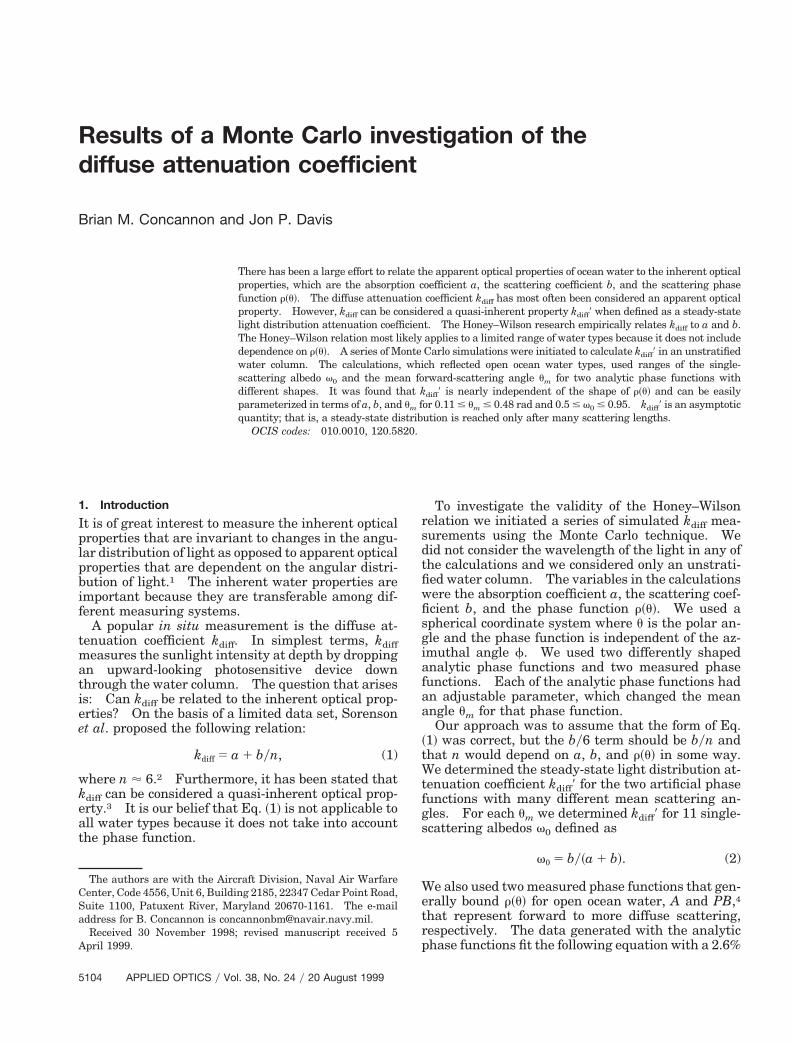
Finally we plotted a from the previous step versus v0and found that a decreasing, linear relationship ex-isted. In Fig. 5, a is plotted versus v0 for the twoanalytic phase functions. In Eq. ~3! a simple functionis written to describe kdiff9 in terms of a, b, and um.

To check the validity of the data generated with theanalytic phase functions we performed the same cal-culations using two measured phase functions. Us-ing the calculated um for each phase function and thelyn values derived from the Monte Carlo calculationsfor assumed a and b, the results, plotted in Fig. 6,show that the data generated with measured phasefunctions agree well with the derived fit from Fig. 5.

As an additional check on the calculations, we rananother set of simulations using a value of b 50.03ym; the first set of calculations used b 5 0.12ym.

Fig. 2. A and PB measured phase functions.

Fig. 3. ~kdiff 2 a! and a three parameter fit.

Fig. 4. lyn versus um for two scattering albedos.

vt

mswuw

d

oH

e

l

The a~v0! data points generated were also plotted inFigs. 5 and 6. It is clear that lyn has little depen-dence on the ratio of a and b separately but, instead,depends on v0.

In our simulation, kdiff approached a steady-statealue only after many scattering lengths. To inves-igate how kdiff approached kdiff9 under more realistic

conditions such as a rough water surface or a cloudyday, we conducted a simulation in which we initial-ized the photons to represent a diffuse, extended lightsource. We found that kdiff9 was approached after

any fewer scattering lengths than the perfectlyunny day and flat surface simulations. However,e found that it was easier to fit the data generatednder the sunny day and flat surface conditionshere at zero depth kdiff 2 a 5 0.

4. Discussion and Conclusion

It has been shown through Monte Carlo techniquesthat the steady-state light distribution attenuationcoefficient kdiff9 can be written simply as

kdiff9 5 a 1 ~1.43–1.17v0!um b, (3)

where a is the attenuation coefficient, b is the scat-tering coefficient, and um is the mean angle of thescattering phase function. This result is insensitiveto the details of the phase function: Use of the value

Fig. 6. Results from measured phase function data.4

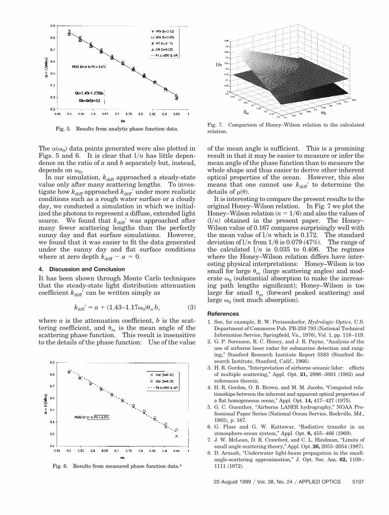
of the mean angle is sufficient. This is a promisingresult in that it may be easier to measure or infer themean angle of the phase function than to measure thewhole shape and thus easier to derive other inherentoptical properties of the ocean. However, this alsomeans that one cannot use kdiff9 to determine the

etails of r~u!.It is interesting to compare the present results to the

riginal Honey–Wilson relation. In Fig. 7 we plot theoney–Wilson relation ~n 5 1y6! and also the values of

~lyn! obtained in the present paper. The Honey–Wilson value of 0.167 compares surprisingly well withthe mean value of lyn which is 0.172. The standarddeviation of lyn from 1y6 is 0.079 ~47%!. The range ofthe calculated lyn is 0.035 to 0.406. The regimeswhere the Honey–Wilson relation differs have inter-esting physical interpretations: Honey–Wilson is toosmall for large um ~large scattering angles! and mod-rate v0 ~substantial absorption to make the increas-

ing path lengths significant!; Honey–Wilson is toolarge for small um ~forward peaked scattering! andarge v0 ~not much absorption!.

References1. See, for example, R. W. Preisendorfer, Hydrologic Optics, U.S.

Department of Commerce Pub. PB-259 793 ~National TechnicalInformation Service, Springfield, Va., 1976!, Vol. 1, pp. 118–119.

2. G. P. Sorenson, R. C. Honey, and J. R. Payne, “Analysis of theuse of airborne laser radar for submarine detection and rang-ing,” Stanford Research Institute Report 5583 ~Stanford Re-search Institute, Stanford, Calif., 1966!.

3. H. R. Gordon, “Interpretation of airborne oceanic lidar: effectsof multiple scattering,” Appl. Opt. 21, 2996–3001 ~1982! andreferences therein.

4. H. R. Gordon, O. B. Brown, and M. M. Jacobs, “Computed rela-tionships between the inherent and apparent optical properties ofa flat homogeneous ocean,” Appl. Opt. 14, 417–427 ~1975!.

5. G. C. Guenther, “Airborne LASER hydrography,” NOAA Pro-fessional Paper Series ~National Ocean Service, Rockville, Md.,1985!, p. 167.

6. G. Plass and G. W. Kattawar, “Radiative transfer in anatmosphere-ocean system,” Appl. Opt. 8, 455–466 ~1969!.

7. J. W. McLean, D. R. Crawford, and C. L. Hindman, “Limits ofsmall angle scattering theory,” Appl. Opt. 26, 2053–2054 ~1987!.

8. D. Arnush, “Underwater light-beam propagation in the small-angle-scattering approximation,” J. Opt. Soc. Am. 62, 1109–1111 ~1972!.

Fig. 5. Results from analytic phase function data.

Fig. 7. Comparison of Honey–Wilson relation to the calculatedrelation.

20 August 1999 y Vol. 38, No. 24 y APPLIED OPTICS 5107