Clemson UniversityTigerPrints

All Dissertations Dissertations

8-2008

RESTRICTIONS ON CREDIT: A PUBLICPOLICY ANALYSIS OF PAYDAY LENDINGPetru StoianoviciClemson University, sstoian@clemson.edu

Follow this and additional works at: https://tigerprints.clemson.edu/all_dissertations

Part of the Economics Commons

This Dissertation is brought to you for free and open access by the Dissertations at TigerPrints. It has been accepted for inclusion in All Dissertations byan authorized administrator of TigerPrints. For more information, please contact kokeefe@clemson.edu.

Recommended CitationStoianovici, Petru, "RESTRICTIONS ON CREDIT: A PUBLIC POLICY ANALYSIS OF PAYDAY LENDING" (2008). AllDissertations. 276.https://tigerprints.clemson.edu/all_dissertations/276

RESTRICTIONS ON CREDIT: A PUBLIC POLICY ANALYSIS OF PAYDAY LENDING

A Dissertation Presented to

the Graduate School of Clemson University

In Partial Fulfillment of the Requirements for the Degree

Doctor of Philosophy Applied Economics

by Petru Stelian Stoianovici

August 2008

Accepted by: Michael T. Maloney, Committee Chair

Cotton M. Lindsay Robert D. Tollison

John T. Warner

ii

ABSTRACT

Using state level data between 1990 and 2006, I find no empirical evidence that

payday lending leads to more bankruptcy filings, which casts some doubt on the debt trap

argument against payday lending. I capture the intensity of the payday lending activity in

a state by the number of payday lending stores.

I control for restrictions on payday lenders by including into the analysis six

variables that I construct that rank legislative provisions across states and across time.

iii

DEDICATION

To all that stayed close to me through good and bad times.

To all who made and make free inquiry possible, to all who strove and strive to

push the limits of understanding.

iv

ACKNOWLEDGMENTS

I thank my committee members for their continuous support, and encouragement.

Mike Maloney has been an inspiration to me. He is everything a professor should seek to

be.

I thank the Economic Department at Clemson University and the Earhart

Foundation for their financial support during my years in graduate school.

Special thanks go to Adi Stavaru for being a steady friend, and Patrick

McLaughlin, and Tim Wiater for making me feel welcome in the U.S.

v

TABLE OF CONTENTS

Page

TITLE PAGE....................................................................................................................i ABSTRACT.....................................................................................................................ii DEDICATION................................................................................................................iii ACKNOWLEDGMENTS ..............................................................................................iv LIST OF TABLES.........................................................................................................vii LIST OF FIGURES ......................................................................................................viii CHAPTER I. INTRODUCTION .........................................................................................1 II. BACKGROUND ON PAYDAY LOANS AND WELFARE

EFFECTS OF CREDIT RESTRICTIONS ..............................................3 Background on payday loans ...................................................................3 Welfare effects of credit restrictions........................................................7 III. LITERATURE REVIEW ............................................................................12 IV. DATA AND THE EMPIRICAL APPROACH ...........................................24 Data sources and Legislative variables ..................................................35 V. DO PAYDAY STORES LEAD TO HIGHER

BANKRUPTCY INCIDENCE? ............................................................41 Difference in difference (DID) estimation.............................................43 Granger causality analysis .....................................................................49 VI. CONCLUSIONS..........................................................................................55

vi

Table of Contents (Continued)

Page

APPENDICES ...............................................................................................................57 A: Payday lending stores members of The Community

Financial Services Association of America ...........................................58 B: Personal bankruptcy filings..........................................................................59 C: Summary of variables ..................................................................................61 D: Coding Criteria for the State Payday Lending Legislation

Restriction Variables..............................................................................63 E: DID estimation: bankruptcy filings vs. payday lending stores ....................67 F: DID estimation: bankruptcy filings vs. payday lending stores

(divorce rate omitted).............................................................................69 G: Akaike Information Criterion (AIC) optimal lag structure..........................71 H: Summary of Granger causality between personal total

bankruptcy filings and payday lending stores........................................72 I: Summary of Granger causality between personal chapter 7

bankruptcy filings and payday lending stores........................................74 J: Summary of Granger causality between personal chapter 13

bankruptcy filings and payday lending stores........................................76 K: Granger causality test between payday lending stores and

personal bankruptcy filings (AIC lag structure) ....................................78 L: Granger causality test between payday lending stores and

personal bankruptcy filings (parsimonious lag structure)......................81 REFERENCES ..............................................................................................................83

vii

LIST OF TABLES

Table Page 1 Simple Granger causality tests between personal

bankruptcy filings and the number of payday stores .............................51

viii

LIST OF FIGURES

Figure Page A-1 The number of CFSA stores (level) .............................................................58 A-2 The number of CFSA stores

(per a hundred thousands persons).........................................................58 B-1 Total personal bankruptcy filings

(per a thousand persons) 1990-2006 ......................................................59 B-2 Chapter 7 personal bankruptcy filings

(per a thousand persons) 1990-2006 ......................................................59

B-3 Chapter 13 personal bankruptcy filings (per a thousand persons) 1990-2006 ......................................................60

1

CHAPTER ONE

INTRODUCTION

From a normative point of view, the interference of the government into voluntary

transaction has to have one of two main goals: a Pareto improvement, or enhancing social

equity. If the public policy is not intended to increase efficiency, then it can be justified

as a means to transfer wealth, and one can engage into a political economy analysis of the

factors that lead to that particular policy, and its costs. Since all policies have costs, a

second concern is to what extent the government intervention in the form of enacted laws

and regulations achieves the proposed goals.

In this paper, I analyze the market for a form of short-term credit, known as

payday lending. I address the question of whether the presence of payday lending stores

has negative welfare implications in the communities where they are present.

Using state level data between 1990 and 2006, and two different empirical

approaches, I find that there is no empirical evidence that payday lending leads to more

bankruptcy filings - a measure of consumers’ welfare. This suggests that there is no

statistical evidence to support the circle of debt argument against payday lending.

I use the variation in the state laws during the same period to identify important

payday lending restrictions that influence payday lenders presence. Based on variation

across states and across time in restriction provisions, I construct six variables that

capture price restrictions, licensing related or entry restrictions, and other business

practice restrictions. These variables rank the provisions across states and time. I find

2

that the main restriction that influences the presence of payday lenders is the price

restrictions.

Chapter two gives a short background on payday lending, and some of the

potential welfare effects of regulating the credit market. In the next chapter, I review the

literature. I discuss the data and the empirical approach in chapter four. I investigate

whether payday lending stores lead to higher bankruptcy incidence in chapter five.

Chapter six concludes.

3

CHAPTER TWO

BACKGROUND ON PAYDAY LOANS AND WELFARE EFFECTS OF CREDIT RESTRICTIONS

Background on payday loans

A payday loan (also known as deferred deposit advance or loan, cash advance,

payday advance) is a single payment unsecured short-term credit of small amounts.

The lender keeps until the maturity of the loan the personal check issued by the

debtor that includes both the principal and the interest (the transaction could also be

based on an agreement authorizing the lender to make an electronic withdrawal from the

borrower checking account on the maturity date).

The lender requires some proof of income (recent pay stabs usually suffice), and a

checking account. The maturity of the check usually coincides with the borrower’s next

paycheck or deposit of funds date. At maturity the check is either deposited by the lender

or the borrower pays in cash to get it back.

The check is not collateral, but acts on the margin as a deterrent to default and

reduces the cost of collection, because returned checks generate farther charges.

A typical two-week $300 cash advance will usually have a $451 charge, which

corresponds to a 390% non-compounding APR.

There is evidence that in fact borrowers take several loans during a year, which

would suggest that to a certain extent a rollover phenomenon is present2.

1 This information comes from industry insiders, and it is consistent with previous studies - for example, “80% of all

payday loans across the country are reportedly less than $300” in Stegman (2007), p. 169, Chessin (2005), or reports - for example, WA state DFI (2006).

4

Elliehausen and Lawrence (2001), Chessin (2005), Stegman (2007), Skiba and

Tobacman (2007) summarize the reasons individuals take payday loans, alternatives

available, and demographic characteristics of payday lending users.

At the beginning of the 1990’s these lending services were provided mainly by

small independent check cashing outlets and pawnshops. Now the industry expanded

significantly, and the providers include large regional or national multi-service providers

(some of them publicly traded)3.

This increase in the industry is consistent with the evolution of the store locations

of the members of the national trade association, The Community Financial Services

Association of America (CFSA), comprised of more than 150 members representing over

half of the payday lending stores4.

As the number of payday lending stores increased in the last 10-15 years, both in

absolute numbers and per capita (see appendix A), reaching today around 23,0005 store

locations nation wide, many states that did not have already restrictions in place, started

to respond in state assemblies.

The enacted payday lending specific restrictions vary greatly across states, from

no significance restrictions, for example in Delaware, to a complete ban in Georgia. In

2004 in Georgia payday lending was declared public nuisance, it was included in the

definition of racketeering - which could bring up to 20 years in prison and fines of

2 See for example Stegman (2007), Chessin (2005).

3 Snarr (2002)

4 www.cfsa.net/about_cfsa.html, accessed on 3/27/2008

5 My own estimate, based on 2007 data from regulatory bodies.

5

$25,000 per transaction -, and it was subject to class-action lawsuits. In addition, the

creditors were barred from collecting the debt, civil penalties of up to triple the amount of

money gained in interest and fees were established, and the proceeds of the loans were

taxed at a rate of 50%6.

The most important restriction on this type of loans seems to be the price ceiling

imposed.

There were several arguments invoked in passing legislative restrictions against

this type of loans, among which7:

� outrageous / abusive charges;

� pushing people into a debt trap (the circle of debt argument);

� targeting military personnel;

� targeting the minorities and the poor;

� irresponsible lending.

The typical 2-week period could be mostly demand (and not supply) driven; for

example, consumers might want a self-imposed constraint. Since in most of the cases the

6 See S.B. 157, Act 440, signed 4/14/2004, effective 5/1/2004.

7 For example, Georgia House of Representatives Daily Report Number 16, February 12, 2004: “Committee members attending hearings on the subject heard horror stories from people, many of whom served in the armed forces, who fell behind on their payments and were pressured into taking out another loan. These new loans carried additional fees and charges, eventually resulting in payoffs that were exponentially larger than their original loans. Additionally, members learned that payday lending institutions were using many loopholes, and association schemes to avoid Georgia’s usury laws, allowing them to charge exorbitant interest rates, some of which climbed as high as 500 percent. […] in order to prevent payday lenders from preying upon the men and women who serve in our nation’s armed services, House members added special restrictions on payday loans to military personnel.”

OCC Advisory Letter 2000-10: “payday lending can pose a variety of safety and soundness, compliance, consumer protection, and other risks to banks. […] The OCC will closely review the activities of national banks engaged or proposing to engage in payday lending, through direct examination of the bank, examination of any third party participating in the transaction under an arrangement described above, and, where applicable, review of any licensing proposals involving this activity. These examinations will focus not only on safety and soundness risks, but also on compliance with applicable consumer protection and fair lending laws.”

6

charges are the same per transaction, the more a person renews a loan (effectively

increasing its maturity) the longer maturity they would want (perhaps realizing that the

constraint they impose on themselves does not work). In other words, we should see that

the maturity is a positive function of the number of rollovers.

It is likely however, that the main reason why payday loans are usually of small

amount with a maturity no longer than two weeks - even in states where the loan and

maturity limits are larger or no limits exist -, has to do with the risk of the loan. It seems

that this is the optimal combination that allows a reasonable assessment of the risk of

default for these subprime individuals, based on the potential source of repayment.

Payday lenders do screen the applicants. Even though the payday lenders might

not pull up the applicant’s credit score from a credit reporting agency (however, some

payday lenders use other external services to verify the applicant - for example,

Teletrack8), they do check the past behavior of the applicant with them and their affiliates

(and in some states with all payday lenders in that state). The proportion of rejected

payday lending applications in Skiba and Tobacman (2007) was about 20%9.

The very small default rate10 for this small unsecured loans, would suggest that

borrowers value the option to come back.

Thus, the argument of irresponsible credit used as proof of lenders preying on

innocent victims (without taking into account the ability to repay) loses its strength.

8 www.teletrack.com/successes/payday.html, accessed on 3/27/2008.

9 Rejection rate of 19.89% = 17.4%*99.6% + (100% - 17.4%)*(100% - 96.9%).

10 Between 1996 and 2004, in Colorado 3.34% of the total loan volume were charged-off Chessin (2005); industry insiders claim that the national average is around 2%.

7

Welfare effects of credit restrictions

Restrictions on credit diminish the ability of individuals to smooth their

consumption in the presence of income or expenditure shocks (like loss of employment,

medical emergency).

Unless they increase the efficiency or the competition, restrictions on a business

activity are likely to lead to increases in costs. In the long-run, since there are no barriers

to exit the industry, these will be passed onto consumers. Morse (2007) argues that the

threat of legislative restrictions acts like a potential barrier, reducing the competitiveness

of the industry below what it could be otherwise.

In addition to direct increases in costs caused by compliance with the rules and

regulations, there is an indirect negative effect on consumers: the uncertainty with respect

to future legislative provisions (based on high recent volatility across states) will make

the expected required returns for the lenders higher than it would be otherwise.

However, there are several reasons why regulating the credit market might

increase the efficiency of that market. For example,

� the presence of market power

� asymmetric information, and externalities

� time inconsistent preferences.

It is hard to convey that there is too much room for misleading in a payday

contract because it is very simple in terms of the costs and structure: there are no hidden

costs. If the borrower keeps his promise to return the loan at maturity, then the cost is

8

just the difference between the value of the check that the lender will deposit at maturity

and the amount that the borrower got when the contract was signed.

Why the borrower does not return the loan at maturity is another story. If his

intention was to cheat on his contract it is not clear that we should take his side just

because he is presumably poorer.

In this context, the circle of debt argument works only if the costs that the default

borrower has to bear are hidden and disproportionately high, and if the lenders would

impose a high minimum amount loan that would make the borrower less likely to be able

to repay it, which is not supported by the evidence.

Paternalism could be justified if the supplier has an information advantage over

the consumer. Suppose the consumer is not "smart enough" to figure out that the loan on

average has to be refinanced, i.e., he accepts a short term interest rate for essentially what

is a medium term loan. To prevent the supplier to use this asymmetry in information to

prey on the borrower, restrictions could be put into place to stop the consumer from

entering contracts that are not in his own interest.

If the borrower does not understand the high costs of the loan, and if he is at the

bottom distribution of the income and financial sophistication, he is more likely to be

unable to repay it at maturity. He will either default or try to refinance. If he will get into

a rollover or renewal of the debt, the result will be a rapid increase in his indebtedness.

This is because payday loans are designed as short term loans, but become increasingly

costly as medium or long term instruments.

9

Posner (1995) argues that “it is difficult to say that all or even most poor or not so

poor people who accept risky credit do so because they have bad judgment” (p. 296). He

points out that in a society that has welfare programs, restrictions on voluntary

transactions can increase efficiency. He suggests that the survival of usury over time can

be explained by our welfare system. Usury laws prevent some of the lending to high-risk

borrowers who are or would be as a result of extra borrowing on welfare. The

restrictions, in this way, would reduce the excess credit. The potential welfare

opportunistic behavior would be mitigated, and the social desired standard of living could

be achieved at a lower cost.

Borrowers are affected differently by restrictions on the ability of the lender to

recover the loan, depending on their probability to default. Barth et al. (1986) point out

that borrowers with relatively low probabilities to default are made worse off by

restrictions on credit because of the resulting higher charges. Borrowers with relatively

higher probabilities to default could be made better off, especially if they act

opportunistically, but whether or not they gain is an empirical matter. Barth et al. (1986)

argue that restrictions on creditor remedies leave the typical borrower worse off.

Brooks (2006) argues that there is a source of negative externality in the fringe

market: since most creditors do not report to credit reporting agencies their credit history

with their customers, they prevent “good” borrowers to move into to the low cost credit

market. He suggests, however, that requiring or encouraging fringe creditors to report

their credit history with their customers might be preferred to preventing fringe credit.

10

If the discounting factor of the future utility depends on the time span to that

future, and not upon the period in which it occurs, the preferences will be time

inconsistent, and the individuals will have self-controlling problems. Strotz (1956)

shows that under these conditions, precommitment could enhance one’s utility.

Individuals with hyperbolic discount functions – for which the instantaneous

discount rate for future consumption falls as the time horizon increases -, have

dynamically time-inconsistent preferences. Constraints on their future behavior - like

limits on their ability to consume -, could improve their welfare.

Laibson (1997) shows that individuals with hyperbolic discount functions could

be better off if they are able to impose liquidity constraints on themselves by investing

into illiquid assets. For them, having access to finance can make them worse-off since it

reduces their ability to commit. His efficiency improvement results hold in general if

there are no unforeseen emergencies.

To summarize, the net welfare effects of restrictions on credit are ambiguous:

a) some individuals will use high cost payday loans until they overcome the bed

times. Even if they borrow often from payday lenders during a period of time, they are

more likely to be left worse off as a result of more restrictions, since credit access will be

reduced; in addition, one of the effects of regulations is an increase in costs and thus in

the price paid. Restrictions on payday lending could stop or discourage people in this

group from engaging in voluntary trade, and could force them to choose a less preferred

alternative (presumably more costly).

11

b) It is quite possible, on the other hand, like with any other market transaction,

that some individuals will make mistakes and will find themselves ex-post in a worse

position than anticipated. Some individuals might, but not necessarily, be left better off

with more restrictions on payday lending (for example, individuals who have self-control

problems). Even for the second group it’s not clear that they would be better off. The

relevant question is what their opportunity cost is, what they would do if more

restrictions on payday lending will leave them out of this market.

From a public policy point of view, the question is not whether there are

individuals who will be made better off by more restrictions, or by less restrictions

(almost certainly the answer is yes to both), but rather which group dominates, what is

the net welfare effect – which is an empirical matter.

12

CHAPTER THREE

LITERATURE REVIEW

Early period is dominated by consumer advocacy studies, which mainly have

correlations and cross-tabulations, and studies which are predominantly descriptive and

legislation focused.

Studies on payday lending often arrive at contradictory conclusions.

Many authors have tried to identify the factors that influence the demand and the

supply for payday loans; for example, Graves (2003), Graves and Peterson (2005),

Stegman and Faris (2003), Burkey and Simkins (2004).

Other researchers try to analyze the industry and the financial performance of

payday loan firms: for example, Stegman and Faris (2003), Flannery and

Samolyk (2005), Morgan (2007), Huckstep (2006).

Others focus on how the consumers are affected by access to payday lending:

Karlan and Zinman (2007), Skiba, and Tobacman (2007), Melzer (2007), Morse (2007),

Morgan (2007), Morgan and Strain (2007), Wilson et al. (2008).

For more details about payday lending industry see Stegman (2007), Mann and

Hawkins (2007).

Johnson (2002) and Chin (2004) recommend harsher federal legislation of payday

lending. Johnson (2002) supports federal, as opposed to state laws, arguing that payday

lenders are predatory because many systematically break the consumer protection laws.

13

However, no empirical work is included to support his conclusions or to show that his

policy proposal increases efficiency or equity. Similarly, Chin (2004) argues that the

state payday lending restrictions are not sufficient to protect the consumers against

abusing practices, and that minimum regulation at federal level is necessary - including a

price ceiling -, based on which states could have harsher rules. He also suggests that

price ceilings are necessary to prevent a recession that could result from excess

borrowing by the high risk group. No formal empirical analysis is provided to show his

proposal as welfare improvement, other than descriptive tabulations.

For military targeting by payday lenders see Graves and Peterson (2005). Using

store locations in 20 states at the end of 2003 / beginning of 2004 they found support for

the hypothesis that payday lenders locate in the proximity of the military personnel.

They argue that this is evidence of military personnel being targeted by payday lenders,

because the distribution of banks around military bases is not similar, and thus, the

distribution of payday lenders in counties or zip codes within three miles of military

bases can not be explained by potential commercial development patterns and zoning

ordinances. Furthermore, they argue that the large area covered makes it less likely (but

not impossible) that demographic characteristics are driving the results.

But this is what we should expect to get. Graves (2003) shows that in

metropolitan Louisiana and in Cook County (Illinois) banks and payday lenders tend to

be located in different areas. This is contrary to Burkey and Simkins (2004), who find

that payday lenders and banks tend to cluster in the same area in North Carolina, which

they interpret as evidence that banks and payday stores are complements, not substitutes.

14

If payday lenders substitute the banks in this market segment, the result that

payday lenders target military personnel is equivalent to stating that banks discriminate

against military personnel by refusing to serve them.

However, the fact that payday lenders are located in the proximity of military

bases is not necessarily something evil, and it does not prove that payday lenders prey on

the military. They could just respond to the demand. The correlation suggests that

military personnel have some characteristics that make them more likely to demand

payday loans. Actually, Graves and Peterson (2005) identify four main characteristics

that make military personnel more likely to use payday loan.

Graves (2003) addresses the question of minority and the poor targeting by the

payday lenders, by analyzing the difference between the distribution of income and

ethnicity between residents in payday lending neighborhoods and neighborhoods without

payday lenders. He finds that payday lenders enter poor and minority neighborhoods at a

lower rate than banks get out of them.

Albeit the econometric analysis is probably too simple (he tests whether there is a

significant difference between the mean of these characteristics), his results weakly

support payday lending industry claims that their success is caused by the under

provision of this market segment by the traditional credit institutions.

However, Stegman and Faris (2003) find that in low and moderate income

communities in Charlotte, North Carolina, payday lenders enter the market before the

banks leave it. But this could be consistent with a scenario in which the banks stopped

15

offering similar products with payday loans before they left the area, and before payday

lending stores entered it.

Stegman and Faris (2003) find race to be a significant factor in explaining the

demand for payday loans. Burkey and Simkins (2004) also find that race is an important

factor in explaining the location of both payday lending stores and banks in North

Carolina.

Even though they have a small effect on default rates, economic and demographic

factors in the neighborhood where the store is located11 do not have a significant effect on

store profitability in Flannery and Samolyk (2005), after the loan volume is controlled

for.

Stegman and Faris (2003) estimate that a measure of rollovers – the percentage of

chronic borrowers – is the second most important variable to the revenues and a proxy for

profits, after the number of clients.

This is in contradiction with the newer study by Flannery and Samolyk (2005),

who use proprietary individual store data from two large payday lenders and show that

store profitability is cost driven. They find that profitability depends on the volume of

loans, but not on the proportion of frequent borrowers (a measure of the degree of

rollover in that store).

Huckstep (2006) argues that the reason for the large number of stores and high

operating costs (that translate in high fees) relative to other lenders is that payday loans

are a product chosen mostly for convenience. Because of this payday lenders compete in

11 And based on Graves and Peterson (2005) - which find that the store managers want to be within three miles from their target demographic – the characteristics of that store customers.

16

local area and have “high density of stores, and keep those stores open beyond normal

business hours” (p. 210-1)

He compares the profitability of seven publicly traded payday lenders against that

of six commercial lenders and Starbucks. The later was chosen because of the similarity

in terms of business model. He finds that the average 7.63% payday lenders profit

margin is lower than both the profit margins of commercial lenders (13.04%) and

Starbucks (9%).

Morgan (2007) constructs a model to test if payday lenders engage in predatory

lending. Assuming the lenders have an information advantage over the borrower and

engage in predatory lending, the lenders would benefit from pushing borrowers into debt

traps. If payday lenders would prey on borrowers, we would expect to find higher debts

in states with higher loan limits, and also higher defaults.

Based on the 1995 and 2001 Survey of Consumer Finance household level data

and on differences in the maximum loan size across states, Morgan (2007) does not find

evidence that the presence of payday lenders lowers the welfare of less educated and

more uncertain income households: even though the debt level is higher, the defaults are

not. This would suggest that payday lenders do not engage in predatory lending.

Melzer (2008) using a 1997, 1999, and 2002 survey of economic hardship

measures, and within state variation in loan access argues that having access to payday

loans leads to “increased incidence of difficulty paying mortgage, rent and utilities bills;

moving out of one’s home due to financial troubles; and delaying needed medical care,

dental care and prescription drug purchases”.

17

He constructs the variable of interest based on the fact that some counties in the

three states that ban payday lending that he considers are close enough to the border of a

state that allows it, so that there is a border effect. In other words, individuals that live in

the border counties of banning states have access to payday lending and those who live

farther from the border within the banning states do not.

One of the problems with his analysis is that in all three states he bases the

analysis on, payday lenders were not explicitly banned. They were absent because of the

small interest rate caps, which affect all small loan creditors12, not only payday lenders.

So, from this point of view, his analysis holds and will have to be interpreted in the same

way if one replaces “payday lenders” with any other small loan lender (like credit unions

etc.).

He tests for the presence of a border effect based on payday lending stores

location information collected in July 2007 from the state regulatory agency.

There are two reasons why he is likely to overstate this cross border effect.

He uses a 25 miles distance to the border of payday store in the allowing state,

and a 25 miles distance to the border in the banning state as cutting points. Graves and

Peterson (2005) show that payday lending store managers want to be within three miles

from their target demographic.

This is consistent with what I have seen in my data: store location patterns seem

to support a relatively small radius of patronizing consumers for each store: for example,

12 Other than banks after the 1978 Supreme Court decision, Marquette vs. First Omaha Service Corp.

18

Ace Cash Express opened a store in Augusta, Georgia less than 1.8 miles away from its

own store.

Second, there is likely an upward bias in the number of payday lending stores

used to test for the border effects. He overstates the presence of payday lenders, at least

in three states. For example, in Kentucky, Rhode Island payday lenders are licensed as

check cashers, but there is no distinction between check casher only and check cashers

that are lenders. Similarly in New Hampshire, where the licensing data are kept at “small

lenders” level, which include payday loans, title loans, and other small loans.

In addition, the intensity of the presence of payday lenders seems to be ignored.

For example, in New Hampshire the number of total small lenders was about 100

(payday lenders are a subset of that).

There is likely sample selection bias that is not addressed: it is not clear that he

chose the three states randomly.

There were other relevant states to be included in the analysis for his chosen time

frame: in total 10 in which payday lending was effectively banned, 11 that had a regime

change.

One might argue that the analysis should be carried out for all the states to see if

his results are spurious.

Morgan and Strain (2007) test the debt trap hypothesis of payday lending by

analyzing the change in the welfare of consumers in states that banned payday lending in

2004 and 2005 (Georgia and North Carolina) relative to states that did not.

19

They find that households in Georgia are worse off as a results of the ban: they

bounce checks more, have more complaints against lenders and debt collectors, and go

bankrupt more often. This suggests that payday lending gives consumers more options,

and banning it reduced the welfare of debtors, by forcing them into more expensive

alternatives, which contradicts the debt circle argument against payday lending. They

find similar results for North Carolina.

Morgan (2007) also finds that cities with a higher density of payday stores and

pawnshops tend to have lower charges on loans, which support the idea that the payday

lending market is competitive.

Morse (2007) uses propensity score matching to identify the communities that are

likely to be cash constraint based on different socioeconomic variables. The

communities that have payday stores and those that don’t have them are similar in terms

of welfare characteristics considered (foreclosures, deaths, drug treatment, and births).

Then he uses the propensity scores to compare the zip level communities that faced a

disaster (wildfire, flooding, storm/hail, earthquake, landslide, and tornado) with similar

cash constraint ones that did not.

He finds evidence that the welfare variables considered are improved after

disaster shocks in the presence of payday lending.

Furthermore, he finds that high bank density (measured relative to the mean) does

not have the same positive welfare effects as payday lending.

Wilson et al. (2008) found similar results in a laboratory experiment that sought to

test how individuals who face similar constraints to those faced by payday loans

20

customers are affected by access to payday loans: “78.1% of the subjects with access to

payday loans benefited from both the existence of and their subsequent use of payday

loans” when they where faced with expenditures shocks (p. 25-6). He also finds that if

the number of loans is above a certain threshold (ten), individuals are less able to absorb

negative shocks than similar individuals that do not have access to payday loans.

Skiba and Tobacman (2007) look at the effect of access to payday loans on

borrowing activity, bankruptcy, and crime. They do not find any effect on crime, but

they find that higher access to payday loans leads to higher frequency of borrowing.

They also find suggestive but inconclusive evidence that access to payday loan

credit (measured by the applicants’ payday loans approval) increases chapter 13

bankruptcy filing rates, which is in contradiction with this paper’s results.

However, there are several reasons why their results might be problematic.

What they are actually addressing is the impact of access to payday loan credit

(measured by the outcome of the first payday loan application, accepted or rejected) on:

� subsequent payday-loan applications;

� pawn loan borrowing;

� personal bankruptcy petitions.

This is different in important ways than access / denial of credit induced by

regulations. What they capture is the behavior of two groups of individuals that have

different relevant characteristics: some are considered too risky by the payday lenders,

and the others are not.

21

If payday lending has any welfare effects (positive or negative) - at least in terms

of policy implication -, the relevant population for analysis is not all applicants, but rather

approved applicants.

In other words, if, for example, we are interested to see if payday lending leads

borrowers into a cycle of debt (and eventually to bankruptcy), those who apply but are

rejected should not be included in the analysis (even if they are cash strapped).

The access to payday credit is estimated based only on the success of the

application to the payday lender that they base their analysis on. In most instances, an

individual could borrow from several payday lenders. If payday borrowing has any

effects on bankruptcy etc., then what’s relevant is the overall payday history, not only the

history with one payday lender.

Furthermore, they use only the outcome of the first application as a measure of

access to payday credit. It is likely that conditional on being approved once, the

subsequent history is more important.

When they analyze the effects on bankruptcy, they looked at bankruptcy filings in

three Texas Districts, based on which they matched the individuals in their data set.

However, we can not tell a priori if they misrepresented or they overrepresented the

proportion of those who filed for bankruptcy and had borrowed from a payday lender.

They use the data from a payday lender which also offers pawn loans, and we do not

know how representative that lender is for the whole payday lending industry. There are

a few major players at the national level, and we know that their data do not come from

22

the biggest one (Advance America), which does not offer pawn loans, and has more than

twice the payday lending stores than the second biggest chain13.

Another source of problem in their study is that their data set is truncated. They

have payday transaction data for 4 years, from 9/2000 to 8/2004. The pawnshop data

spans from 1/1997 to 11/2004 and is for the same company. The bankruptcy data are

from 1/2001 through 6/2005, the arrests data are from 2000 to 2004. They do not seem to

address this problem (the history of a lot of individuals does not start with their data set,

so a lot of the relevant information is missing, and is not missing consistently across

individuals).

This paper contributes to the literature on payday lending in several ways.

Most of the papers study the effects of payday lending based on access to payday

lending, without a measure of the intensity of the industry.

As far as I am aware, only Graves (2003), Graves and Peterson (2005), Burkey

and Simkins (2004) and Stegman and Faris (2003) incorporate the number of payday

lending stores into the analysis.

Graves and Peterson (2005) use store locations in 20 states at the end of 2003 /

beginning of 2004 to see if payday lenders tend to be located in the proximity of the

military personnel.

Graves (2003) analyzes the spatial distribution of banks and payday lenders in

metropolitan Louisiana, and in Cook County, Illinois.

13 My own estimate, based on 2007 data from payday lenders and regulatory bodies.

23

Burkey and Simkins (2004) try to explain the location of both payday lending

stores and banks in North Carolina in 1999 and 2000 based on demographic

characteristics.

Based on Charlotte, North Carolina data in 1999 and 2000, Stegman and

Faris (2003) use the number of payday lending stores to model payday lenders revenues.

They also use these data to see how payday lending stores are located relative to the

banks.

This paper is similar with Skiba and Tobacman (2007) who have payday

transaction data for 4 years, but they measure the effects of being granted a first payday

loan.

In this paper I use the number of payday lending stores for each state between

1990 and 2006 to capture the effect of the intensity of the industry on the welfare of

consumers, measured by the bankruptcy filings. I try to capture the intensity of the

presence of payday lending activity through the number of payday stores.

I also have a longer panel data, which capture the outset of the industry, and in

addition I measure the effects not only of the presence of payday lenders, but also of the

change in the relevant legislation.

24

CHAPTER FOUR

DATA AND THE EMPIRICAL APPROACH

Ideally, the welfare effects of payday lending should be analyzed by tracking over

time the individuals who are using this type of loans with respect to different measures of

welfare.

Data limitations however do not allow me that.

Instead, I use the variation in payday lending legislation and the number of

payday lending stores across time and states to assess the aggregate effects at state level.

Given the prevalence of repeated borrowing14, since payday loans users accept to

borrow with such a relatively high cost, it is likely that they don’t have other less

expensive alternatives. Elliehausen and Lawrence (2001) show that more than 60% of

payday loans users did not use their bank cards because they did not have enough

available credit. This means that individuals who fit the profile of a payday loan

borrower are likely to be more exposed to negative shocks. This is consistent with Skiba

and Tobacman (2007) who find that the bankruptcy rate of payday loan users is ten times

higher than the national average.

For a review of the bankruptcy procedure see, for example, Luckett (1988) or Fay

et al. (2002).

There are two main ways in which a debtor could get some relief under the

bankruptcy laws: file for liquidation of his non-exempt assets under chapter 7, or file

14 For example Stegman (2007), Chessin P. (2005).

25

under chapter 13. Under chapter 7 debtors’ non-exempt assets are sold and any

unsecured debts that can not be covered from the proceeds are discharged, with no other

obligation for the filer. Under chapter 13 the debtor keeps his current assets, but

promises to repay his debt (or a fraction of it) out of his future income.

Borrowers who are pushed into repeat borrowing are more likely to file for

chapter 7, especially if they don’t have many assets (if you feel that you got somehow

cheated, you are more likely to want to have the debt discarded).

Gross and Souleles (2002) argue that the default costs have decreased; in addition

the filer could ask in the petition to have the court filing fees waived.

The main question addressed in this paper is whether payday lending directly or

indirectly contributes to an increase in bankruptcy.

Bankruptcy is a reasonable measure of welfare.

Payday lending could lead on the margin to bankruptcy especially if the debt trap

is significant (Morgan, 2007).

Intuitively, the circle of debt argument might be flawed because the industry can

not built itself in the long run seeking to bankrupt its customers (if that would be the case,

its customer base market will shrink).

Bankruptcy is associated with real welfare problems for consumers.

In Himmelstein et al. (2005), “during the two years before filing for bankruptcy

40.3% had lost telephone service; 19.4% had gone without food; 53.6% went without

needed doctor or dentist visits because of the cost; and 43.0% had failed to fill a

prescription, also because of the cost.” After filing for bankruptcy, “about one-third of

26

debtors continued to have problems paying their bills. […] Because of the bankruptcy on

their credit reports, after about 7 months from the filing, they had already been turned

down for jobs (3.1% of debtors), mortgages (5.8%), apartment rentals (4.9%) or car

loans (9.3%).”

In states with higher bankruptcy exemptions levels, low-income households tend

to have less credit, and pay higher interest rates on automobile loans than similar

borrowers in states with low exemptions Gropp et al. (1997).

To capture the relationship between payday lending and bankruptcy, two

estimation procedures are employed: a difference in difference estimation and a Granger

causality test between payday lending stores and personal bankruptcy filings.

Using the variation in legislation across states and across time, and assuming that

there are no significant and systematic cross-border effects, two groups of states have

been identified:

� the control group: states with no change (where payday lenders were not

present at all, or were present during all periods), and

� the treatment group: states that have seen a change in the presence of

payday lender (they entered or exit during the period).

More on the exact specifications in chapter five.

The factors that influence bankruptcy filings have not been unambiguously

determined in the literature. In addition, factors that explain the variation across time and

27

space based on bankruptcy petitioners characteristics and interviews are not consistently

significant in studies that use aggregate filings.

Legal environment is important in Fay et al. (2002), Domowitz and Sartain

(1999), but not in Domowitz and Eovaldi (1993), Buckley and Brinig (1998).

Social and economic shocks are significant in Himmelstein et al. (2005)

(medical), Domowitz and Sartain (1999) (medical), Domowitz and Eovaldi (1993),

Agarwal and Liu (2003) (unemployment, medical, divorce), but are not in Fay et

al. (2002) (medical, unemployment, divorce).

Credit card or consumption related debt play a role in Domowitz and

Sartain (1999), Luckett (1988), and social norms in Gross and Souleles (2002), and

Buckley and Brinig (1998).

Himmelstein et al. (2005), based on their own 2001 survey of debtors in

bankruptcy courts, find that about half of the individuals surveyed claimed that the main

reason for their personal bankruptcy was medical.

In addition, it did not take too much: for those that claimed medical reasons as the

main cause of bankruptcy, the out-of-pocket costs since the start of illness were on

average close to twelve thousands dollars, and the average out-of-pocket medical costs

(excluding insurance premium) were close to thirty seven hundred. Furthermore, 75.7%

had insurance at the onset of illness, 60.1% had private coverage, but one third of them

lost coverage during their illness. Gaps in coverage were present over the two years

previous to the filing for 38.4% of them, and 32.6% of debtors claiming a medical

28

problem as the main cause for bankruptcy were uninsured at the time of filing for

bankruptcy.

The median income in the year prior to bankruptcy filing was $25,000.

Domowitz and Sartain (1999) based on a sample of two 1980 quarters of

bankruptcy filings in five court districts found that medical and credit card debt are the

most important contributors to bankruptcy at household level.

Home ownership and exemption levels influence the choice of bankruptcy

chapter. Specifically, home ownership, as expected, increases the probability of choosing

chapter 13 over 7, medical debt has a negative impact on this choice, being married or

employed a positive effect. The less the total debt relative to all claimed exemptions is,

the more likely the filer will chose chapter 7, but this effect is marginally insignificant (t-

value is 1.8).

One of the potential problems of their analysis is that they normalized the

household assets to household income, in spite of the fact that bankruptcy exemptions are

not set relative to income (with the exception of unpaid wages in some states). In

addition, unused exemption levels can not be used across asset categories.

The net benefits from filing under chapter 7 are given by the unsecured debt

discharged in bankruptcy minus the value of non-exempt assets that the households

would have to give up, the legal costs, the negative effect on future access and cost of

credit, stigma costs, the cost of acquiring information about the bankruptcy process and

so on.

29

Fay et al. (2002) analyze the factors that influence the bankruptcy at household

level using Panel Study of Income Dynamics (PSID) data.

Based on variation in exemption levels across states, they find that the financial

benefits from bankruptcy positively influence the probability of filing. Also, that

discharging of debt is the driving factor, and that giving up assets in the process is

insignificant.

Lagged bankruptcy filing in the household’s district has a positive and significant

effect on the probability of filing (less stigma, and lower information costs).

They also find that both the lagged household’s income and the reduction in

income between year t-2 and t-1 are significant and negatively related to the probability

of filing. But they argue that the mis-measurement of the wealth variable (since wealth

data are collected only in five-year increments, they used current income as a proxy for

change in income since the last collection time) makes these results unreliable. Instead

they look to see if adverse events that happened in the previous year have any effect on

filings. They find that having health problems and having spells of unemployment in the

previous year (household head or spouse) have positive but insignificant effects on the

probability of filing. The only adverse factor that was significant and positive at more

than 7.7% level was whether the household head was being divorced in the previous year.

They also control for demographic characteristics: age of the household head, the

head’s education level, family size, home ownership, whether the household owns a

business. These are also assumed to proxy the cost of lost future access to credit as a

30

result of bankruptcy. In addition, they included state or county level variables: state

income growth, state income standard deviation, county unemployment rate.

The authors acknowledge potential measurement errors induced by availability of

unsecured debt and non-housing assets only in five-year increments, but find that this

measurement error does not significantly affect the results.

However, it is possible that the way the financial benefits were constructed had

induced another measurement error in the key variable of their study.

The assets at risk of liquidation are included in many exempt categories

(including unpaid wages). Not including all exemptions might induce a downsize bias in

the financial benefits variable.

They constructed for each year for each household:

FinBen = max[D - max (W - E, 0), 0]

where

FinBen = Financial Benefits from filing

D = unsecured debt

W = household wealth net of secured debt

E = bankruptcy exemption, and it’s the sum of equity in owner-occupied

homes exemption, equity in vehicles exemption, and personal property

applicable to financial assets exemption, plus the wild card exemption

(which allows the exemption of an unused amount of the homestead

exemption - in order not to discriminate against the non-homeowner – and

which can be applied to any asset).

31

This aggregation overstates the size of the assets at risk, since they seem to be

based on the difference between total household wealth net of secured debt and the sum

of different category exemptions. More accurately, the financial benefits should have

been calculated as:

FinBen = max{D – j

sum [max (Wj - Ej, 0), 0]}

where j denotes an exemption category.

This problem is mitigated (but not eliminated since it comes at a cost) if the filer

acts opportunistically before the filing by moving assets between different exempt

categories.

Moreover, even though the benefits for filers under chapter 13 have to be at least

as large as those under chapter 7 (since the filer revealed chapter 13 to be preferred over

chapter 7), the financial benefits are not the unsecured debt discharged, because debt has

to be paid. The benefits are rather in terms of costs saved from an involuntary

liquidation, net of the legal cost and other costs associated with bankruptcy.

The variable FinBen is likely censored in the case of chapter 13 filings.

Another potential problem is that even though the sample size is larger than 55

thousands observations, in their sample there are only 254 bankruptcy filings. In

addition, the PSID filing rate is only about half of the national level.

Agarwal and Liu (2003) argue that the small number of bankruptcy filings in Fay

et al. (2002) likely is associated with too small variation in adverse macroeconomic

variables, and as a result it could explain why they are not able to capture the effects of

the macroeconomic variables.

32

Using quarterly data on personal bankruptcies per capita, from the fourth quarter

of 1960 to the first quarter of 1985, Domowitz and Eovaldi (1993), after adjusting for the

joint-filing provisions of The Bankruptcy Reform Act of 1978, argue that the main cause

of the increase in personal bankruptcy filings was not the change in the bankruptcy law,

but rather “business-cycle conditions, expectations phenomena, and demographic trends”

(p. 805).

Using random samples of chapter 7 and 13 individual cases filed in five

bankruptcy court districts from October 1978 through March 1979 and in April-

September 1980, and a different empirical approach, they also find that the change in the

law induced by the Bankruptcy Reform Act of 1978 did not have significant effects on

filings, once business-cycle factors are considered.

White (1998) argues that bankruptcy filings are much lower than what they could

be based solely on the benefits from filing. This could be explained in part by two

factors. Asymmetric information between creditors and debtors results in lower

collection efforts by creditors (creditors do not try to collect on default loans in all

instances), and as a result fewer filings take place. In addition, the availability of the

bankruptcy in the future is valuable to the debtors.

Using proprietary 1995-2001 monthly credit card data at individual level from a

national issuer, and estimating duration models of delinquency, Agarwal and Liu (2003)

find county unemployment rate to be an important factor in explaining delinquency.

33

They also find state average income statistically significant and negative, the

number of individuals with no medical coverage in the state to be positive and

significant, divorce rates marginally significant.

Even though they control for state specific legal variables, including homestead,

property and garnishment exemption levels, they do not report the significance and sign

of the coefficients on these variables.

Based on different specifications that include different lags of unemployment rate

and change in unemployment rate, they argue that the level of unemployment rate is more

important than the change in unemployment rates. However, this misinterprets their

specifications, because they actually estimate the effects of different lags.

For example,

their (12) β1*U(t-6)+ β2*∆U[(t-3)-(t-6)] = β2*U(t-3) + (β1 - β2)* U(t-6) =

= 0.0032 U(t-3) + 0.01461 U(t-6)

Luckett (1988) analyzes the bankruptcy legislative changes and presents a

summary of the most important literature on bankruptcy before the late 1980s. He argues

that consumption related debt is likely a key factor in explaining the rising trend in the

personal bankruptcy filings after WWII.

Buckley and Brinig (1998) attribute most of the variation in district filings to

changes in social norms. Their data cover chapter 7 and chapter 13 annual filings

between 1980 and 1991. The legal variables used (an estimate of the maximum real

value of assets exempt from seizure in Chapter 7 by unsecured creditors, and a dummy

that captures the bankruptcy court district enforcement of safeguards against debtor

34

misbehavior under Chapter 13) do not appear to have a significant effect on filings. They

suggest that econometric analysis of bankruptcy filings should include social variables

predictors.

They also argue that one period lag is the reasonable lag of the independent

variables.

Gross and Souleles (2002) identify two explanations for the trends in personal

bankruptcy filings and delinquency rates on credit cards: the deterioration in the risk

composition of borrowers, and the increase in borrowers' willingness to default as a result

of a decrease in the default costs, including social, information, and legal costs. They use

a proprietary individual credit card accounts data covering 1995-97 from several different

card issuers, which have many variables that control for risk.

They argue that even though risk variables are highly significant in predicting

bankruptcy, the changes in the risk composition and other standard economic variables

alone are not enough to explain the dynamics of defaults and bankruptcies. The decline

in default costs (like social stigma or information costs) seems to be empirically

important.

Personal bankruptcy filings graphs are presented in appendix B. All demographic

and shock variables included in the bankruptcy analysis are listed in chapter five, and

summarized in appendix C.

35

Data sources and Legislative variables

Population, percent of individuals not covered by private or government health

insurance, poverty rates data come from U.S. Census Bureau.

Poverty rates were available only for 1994-2006. In the regressions where

poverty rates are used on the right hand side, this is the implicit time span of the analysis.

Income data comes from the Bureau of Economic Analysis (within the U.S.

Department of Commerce).

Unemployment and CPI data are from the Bureau of Labor Statistics (within the

U.S. Department of Labor).

Divorce data are from the National Center for Health Statistics. No data for 1992

were available; also some states and years are missing (total missing observations is 170

out of 867).

Consumer Credit Outstanding data source is the Fed.

The number of payday lending stores comes from The Community Financial

Services Association of America (CFSA), the industry trade association. More details on

this variable are provided in chapter five.

Personal bankruptcy filings data are from Administrative Office of the U.S.

courts.

There are three relevant groups of legal payday lending restrictions identified in

this paper:

A) Price restrictions

B) Licensing / entry restrictions

36

C) Business practice restrictions

Price restrictions are mainly fee limits.

Licensing / entry restrictions are mainly bond and net assets requirements, which

are likely to have at least two opposing effects on consumers: act as potential entry

barriers into the market, hence potentially less competition, and secondly making

reputation more important.

Reputation might play a role if there are informational asymmetries between the

consumers and the loan providers.

Suppose, as I mentioned before, the supplier has an information advantage over

the consumer (the consumer is not "smart enough" to figure out that the loan on average

has to be refinanced, i.e., he accepts a short term interest rate for essentially what is a

medium term loan), and uses this asymmetry in information to prey on him. A bond

might reduce the problem of supplier adverse selection in the market.15

In addition, for a given expected rate of return for this business, by directly

increasing the costs of operation through licensing like fees, and through immobilizing

some capital with lower return (the bond), they contribute to higher consumer prices.

Business practice restrictions lead to increases in the production costs.

Any increase in the costs of providing the services will be shared (depending on

the relative elasticities of demand and supply) between the consumers and producers.

There are no compelling reasons to believe that the supply side is not elastic enough in

15 If that would be the case we would expect the public payday lenders to be relatively more supportive of pro-bond restrictions than non public payday lenders.

37

the long run. Thus, ultimately the increase in the costs induced by the regulation will fall

mainly on the consumers.

The legislation considered is just at state level. It does not include any national or

local restrictions on the business considered. However, national level restrictions that

affect payday lenders in the same way regardless of the state are captured in the time

fixed effects.

Restrictions at the local level, like city zoning laws, shape both the size and

location of the stores.

Changes in payday lending regulation at national level affect businesses in

different states differently, depending on the state and local rules in place at that time.16

The relevant explicit or equivalent payday lending legislation was identified based

on information from:

� state legislature web sites

� the state agency that regulates this industry web sites

� LexisNexis Academic (main source for annotated statutes)

The information was cross referenced with government agencies reports, National

Conference of State Legislatures data, industry reports, newspaper articles at different

times from various sources.

16 During the period analyzed, there is only one significant change at the national level that affected states differently: effective 7/1/2005, FDIC changed its payday loans guidelines, in an attempt to discourage long term debt cycles: “banks should ensure that payday loans are not provided to customers who have had payday loans outstanding from any lender for a total of three months in the previous 12-month period”.

In 2/2006 FDIC advised FDIC insured banks that they could no longer offer payday loans through marketing and servicing agents.

38

The relevant payday lending provisions were extracted from the current

legislation for all U.S. states. This allows me to obtain a ranking of payday lending state

restrictions across states.

To capture the dynamics of payday lending state legislature activity, the enacted

state laws were tracked back to 1990.

When the text of the laws that modified the provisions that affect payday lending

was not available on-line from the state legislature or the state agency that regulates the

industry, the legislative changes were inferred in two ways.

a) If annotated statutes for that state were available, the information was obtained

by comparing the provisions in the statutes in two adjacent years, before and after a

known enacted bill back to the 1991 statutes (the oldest LexisNexis on-line statutes).

b) If annotated statutes were not available, the information was inferred by

comparing the statutes provisions that affect payday lending from the last available law,

in each year back to the 1991 statutes.

Each legislative variable was constructed to reflect a ranking across states and

time of state legislative restrictions on payday lending.

This was accomplished by extracting first, and then tabulating the relevant

provisions on each key issue, for all states and for all years. Then the coding rules were

subjectively decided so that they create a ranking of payday lending restrictions

consistent across states and across time. The exact coding criteria used are described in

appendix D.

39

The legislative variables are constructed such that a larger number means more

restrictions.

When a relevant provision in the law became effective during the year, the index

value for that variable for that year changes proportionally with time of the year in which

the new change had effects.

For example, in 2004, the maximum charges for a three hundred dollars 14-day

payday loan in Kansas were about $23. Based on the rules described in appendix D, the

variable “Max charge restrictions” was coded in 2004 for Kansas as 4.

In 2005 there was enacted a law that changed the maximum charges for a three

hundred dollars 14-day payday loan in Kansas to about $45. This act was effective

7/1/2005. Using the same algorithm, after this change, “Max charge restrictions” was

coded as 3.

For 2005, “Max charge restrictions“ was coded as

3.5 ≈ [4 * (12/31/2005 - 7/1/2005) + 3*(7/1/2005 - 12/31/2004)] / 365 =

= (4* 182+ 3*183) / 365.

In rare instances when the exact effective date was not known, the law was

considered effective 7/1.

Georgia, with its S.B. 157 effective 5/1/2004, is the only state that during the

period analyzed explicitly and purposely banned payday lending. As a result, for Georgia

all legislative restriction variables after the effective date of the bill (for 2004 I weighted

for the proportion of the year in which it was effective, as described above), were

attributed maximum restriction values.

40

When the legislative changes or specific provisions for loans similar to payday

loans were not identified, the variables were left missing (70 out of 867 observations).

When there was no payday lending specific legislation, even if payday lenders did

not operate in the state at that time, the provisions that govern a short-term unsecured

loan that have the most favorable for the lender interest restrictions were used.

41

CHAPTER FIVE

DO PAYDAY STORES LEAD TO HIGHER BANKRUPTCY INCIDENCE?

In this paper I try to see if there is any relationship between payday lending and a

measure of consumer welfare, personal bankruptcy filings.

The number of payday stores might be an appropriate measure of the industry size

because the loans are of small amount, with very short maturity. Flannery and

Samolyk (2005) find that the high charge is justified by the fixed operating costs and loan

loss rates, Chessin (2005) finds that the default rate is small (65% of the default rate on

credit cards).

For payday loans more volume requires more workers, i.e., there are relatively

smaller economies of scale than, for example, a bank. This could also explain why the

payday lenders usually increase in size by increasing their number of their locations.

This seems to be consistent with data: as I have mentioned before, Ace Cash

Express opened a store in Augusta, GA less than 1.8 miles away from its own store.

In 2003, 85% of the firms listed in Yellow Pages under SIC "6141-01 Loans" and

"6099-03 Check cashing services" (where payday lending were typically included) had

1-4 employees, 96% 1-9 employees. These SIC’s do not include credit unions,

pawnshops, tax return preparation services, savings and loans associations, trust

companies, other depository institutions.

The number of payday lending stores was not available for years prior to 2006.

Instead, I use as a proxy the number of payday lending stores member of CFSA for each

42

year and state, which was constructed based on CFSA stores that were in business in

March 2006 and the year in which each store was established.

This variable has two potential measurement error sources:

� survivorship bias (it does not include CFSA stores closed); but since the

industry experience mainly expansion, this is likely not that much of a

problem;

� non-completeness bias (it does not include non-CFSA members).

The second is a problem only if CFSA membership is systematically different

across time and across states. I do not have any reasons to believe that that might have

happened.

Furthermore, I try to assess the potential bias empirically: the correlation

coefficient between CFSA stores in 2006, and the actual number of payday stores (based

on my own estimate from regulatory agencies) was 0.9046. If I exclude the states with

no payday lending stores, the correlation coefficient becomes 0.8912. This would suggest

that using CFSA data might be a reasonable approach.

To capture the relationship between payday lending and bankruptcy, I use two

estimation procedures: a difference in difference estimation, and to reinforce the results, a

Granger causality test between payday lending stores and personal bankruptcy filings.

43

Difference in difference estimation

Using the variation in legislation across states and across time, and assuming that

there are no significant and systematic cross-border effects, three groups of states have

been identified:

� states with no payday stores during the entire time span (7 states),

� states with payday stores during the entire time span (19 states), and

� states which did not have payday stores in some periods, but had payday

stores in other periods (24 states).

To estimate the effect of presence of payday lending store a difference in

difference estimation is used. For estimation purposes the states are grouped into two

categories:

� the control group: states with no change (where payday lenders were not

present at all, or were present during all periods), and

� the treatment group: states that have seen a change in the presence of

payday lender (they enter or exit during the period).

A dummy variable, Change, is created to separate the control and treatment

group. For the control group Change takes value 0 for all years. For the treatment group,

change is equal to one. To summarize, for each state and year, Change takes the values:

0: payday lenders were not present in all years in that state

0: payday lenders were present in all years in that state

1: payday lenders were not present in that year in that state, but they where

present in that state in other years

44

1: payday lenders present in that year in that state, but they where not present in

that state in other years

The model can be summarized as:

Yi,t = α + β1 X1it + β2 X2

it + γ1 D05 + γ2 D06 +

+ γ3 Stores it + γ4

(Stores*Change)it + γ5 Change it + εit (1)

where

i is a state subscript

t is a time subscript, t = 1990, …, 2006

Yi,t is personal bankruptcy filings per one thousand persons

X1

it is a vector of demographic characteristics:

� percentage of population age 65 and over

� the natural logarithm of per capita disposable personal real income (2006

thousands $)

� consumer credit outstanding - disposable personal income ratio (this is

available only at nation level)

� the natural logarithm of the percent population below poverty level

� personal bankruptcy filings per one thousand persons in the previous

period – a proxy for “stigma costs”

X2

it is a vector of shock variables:

� unemployment rate

� not covered by private or by government health insurance (% of

population)

45

� divorce rate

D05 & D06 are dummy variables for 2005 and 2006 to capture the effect of the

Bankruptcy Abuse Prevention and Consumer Protection Act of 2005 -

most of its provisions were effective 10/17/2005 -, which reduced

significantly the debtor protection under chapter 7 liquidation.

Stores is the number of payday lending stores that are members of CFSA (per 1

million persons).

α, γ1, γ2, γ3, γ4, γ5 - coefficients to be estimated.

β1, β2 - vector of coefficients to be estimated.

Notice that the effect on bankruptcy filings of having payday lending stores is

given by:

( 0

1

>

=

Stores

ChangeY - 0

1

=

=

Stores

ChangeY ) – ( 0

0

>

=

Stores

ChangeY - 0

0

=

=

Stores

ChangeY ) = γ4 * Stores

The interaction term in equation (1), (Stores*Change), captures the DID; it is the

variable of interest in the estimation. It will show if the presence of payday stores is

associated with more, less or about the same bankruptcy filings, for states in which the

presence of the payday lending industry changed. For instance, Georgia had payday

lending stores which were driven out by legislation17. The same happened to some states

as a result of the FDIC ruling18.

This model was estimated separately for total personal bankruptcy filings,

chapter 7 personal bankruptcy filings, and chapter 13 personal bankruptcy filings. The

17 See footnote 6 above.

18 See footnote 16 above.

46

results are presented in appendices E and F. I have tested for the presence of fixed19 and

random20 effects; based on Hausman tests, FE models seem to be preferred.

Specifications (1) through (3) include state and time effects, with robust standard errors.

To avoid the problems created by the assumptions about the data generation process (the

assumptions about the error distribution), I also estimate in (4) through (6) bootstrapped

standard errors. This accounts for the specific characteristics of the data.

There is autocorrelation21 and heteroskedasticity22 present in the data. I correct23

for both in specifications (7) through (9). Because divorce rate is missing (total missing

observations is 170 out of 867), to increase precision, I re-run these models without

divorce rate. The results are presented in appendix F. I have also run models that include

poverty rates (which showed up insignificant, and because poverty rates are missing for 4

out of 17 years in my data, I did not include here those estimates24). Different other lag

structures for the independent variables have been tried, and also other logarithm

transformations to allow for nonlinearities; the results (not shown here) were similar.

The different bankruptcy exemptions across states are captured into the state and time

fixed effects.

The estimates are by and large as expected. Consistent with previous literature,

more filings in the past seem to lead to more filings. This can be explained by a

19 F-test with pooled regression model as the baseline for the comparison.

20 Breusch and Pagan LM test for RE with pooled regression model as the baseline for the comparison.

21 Wald test for first order autocorrelation and Arellano-Bond test for higher order autocorrelation.

22 LR test.

23 Using feasible GLS, panel-specific AR(1) autocorrelation structure, and heteroskedastic error structure.

24 Available on request.

47

reduction in information costs, in the stigma and guilt associated with bankruptcy. In

addition, the more people file for bankruptcy the less severe the reduction in credit access

is. I capture these effects by the coefficient on the lag of personal total filings per one

thousand persons which is significant and of the expected sign.

The lifecycle patterns of borrowing and savings would suggest that as people age,

they would tend to rely more on their savings than on credit to finance consumption.

This would suggest that we expect that, everything else the same, the higher the fraction

of population 65 and over the lower the bankruptcy rate. I find that the percentage of

population 65 or over is indeed inversely related to chapter 13 filings, but positively

related to chapter 7 filings. The later result might happen if individuals in retirement

without significant asset or savings face consumption shocks (for example, unexpected

medical expenditures).

Unemployment rate has the expected sign: an increase in unemployment is

associated with more bankruptcy filings.

Health insurance coverage did not show up to be a significant factor in

bankruptcy.

Real per capita disposable income has the expected sign, but it is insignificant.

Buckley and Brinig (1998) point out that “divorce rates might be positively

correlated with bankruptcy rates in two ways. If the social stigma of promise-breaking is

weakened across the board, then divorce and bankruptcy rates might both increase.

Second, an increase in the divorce rate might directly affect bankruptcy rates because

divorce results in financial distress“ (p. 201-2). In addition, they argue that the causation

48

could go as well in opposite direction: “some people go bankrupt because they divorce,

and some people divorce because they go bankrupt” (p. 202).

Fay et al. (2002) suggest that “divorce lawyers often counsel their clients to file

for bankruptcy” (p. 714).

Divorce rates are found to be consistent with the suggestions in the literature:

positively and significantly correlated with chapter 7 filings. Lagged divorce rates are

found to be positively and significantly related to chapter 13 filings.

The coefficient on "Change" – the variable that separates the control and

treatment group - captures the effect on both groups. The coefficient on "Stores"

measures the effect that is not due to the presence of payday lenders.

The coefficient of interest from a public policy25 point of view is

"Stores*Change".

As mentioned above, this is the DID estimator (the effect of the change in

presence of stores). It measures the effect of the presence of payday stores on

bankruptcy filings.

Notice that since we use the number of payday lending stores per one million

persons and not just "laws allow payday lending" or "payday lending stores present in

state" (like in other papers), I also controlling for the intensity of the industry – which

was not done before.

The DID coefficient will show if the presence of payday stores is associated with

more, less or about the same bankruptcy filings.

25 This is the most relevant effect to look at for allowing / banning payday lending.

49

Controlling for the intensity of the payday lending stores, I find that if anything

the presence of payday stores in a state is associated with smaller chapter 7 bankruptcy

filings. The effect is economically very small: chapter 7 filings go down by about 1

filing per 1 million persons.

The presence of payday stores does not seem to have any significant effect on

chapter 13 and total personal bankruptcy filings.

Granger causality analysis

To reinforce these results I test for Granger causality between bankruptcy and

payday lending stores.

Granger (1969) shows that a variable X is causing another variable Y if, given all

available information about Y and other relevant variables, we are able to predict Y better

using X than without it. If adding X to all other available information does not increase

the forecast power for Y, then X does not cause Y.

This implies that if X causes Y, then ∆ X(t) => ∆ Y(t+j), but ∆Y(t) does not lead to

∆X(t+j), for a lag j.

Panel data Granger analysis have to take into account the possible state

heterogeneity in the relationship.

I start first with a simple bankruptcy filings – payday lending stores Granger

causality test (no other variables included) at state level, and then I analyze the

consistency of the results across states. If payday lending causes bankruptcy, then this

relationship should consistently hold also at state level.

50

This simple Granger test at state level could be extended by controlling for other

factors. However, the relatively short period of time of my data (17 periods maximum)

does not allow me this.

By restricting the Granger analysis at state level I will avoid any heterogeneity

problems, but at the same time not all the available information is used (since payday

stores are not present in all the states, and other important variables that could affect the

relationship between bankruptcy and payday lending are not controlled for).

I then repeat the Granger analysis with the pooled data, including economic and

social variables that proved to be important in the DID analysis, and also controlling for

variation in payday lending legislative restrictions across states.

The simple Granger causality test is based on the model:

Bankruptcy filings i,t = ∑=

p

1j

α j *Bankruptcy filings i,t-j +

+ ∑=

p

1j

βj *Stores i,t + ui,t (2)

Stores i,t = ∑=

r

1j

γj *Bankruptcy filings i,t-j +

+ ∑=

r

1j

δj *Stores i,t + vi,t (3)

The appropriate number of lags p, and r were determined using the Akaike

Information Criterion (AIC).

51

The optimal number of lags for each state level is not always the same with the

one that results from the pooled data (see appendix G). However, for total personal

bankruptcy filings, I have done the analysis using both the optimal lag structure

determined at the state level and the optimal lag structure determined with all states

pooled. The conclusions of the Granger causality test did not change.

Under this specification, if payday stores cause bankruptcy, then βj in equation (2)

are different than zero, and γj in equation (3) are zero.

I have run these models by state, and then I have tested for these Granger

causality requirements.

The results are summarized in table 1 below:

Table 1. Simple Granger causality test between personal bankruptcy filings and the number of payday stores

(1) (2) (3) (4)

total total ch. 7 ch. 13

Stores "causes" Bankruptcy, and Bankruptcy

does not "cause" Stores 6 5 6 8

Bankruptcy "causes" Stores, and Stores does not "cause" Bankruptcy

3 7 2 4

Bankruptcy "causes" Stores, and Stores "cause" Bankruptcy

2 1 3 0

Bankruptcy does not "cause" Stores, and Stores do not "cause" Bankruptcy

21 19 21 20

The numbers are number of states

In (2) I used the number of lags that results from AIC at state level (instead from AIC with all data pooled) - see appendix G

The number 6 in column (1) means that in 6 states I failed to reject the hypothesis

that γj were jointly significantly different than zero, and I rejected the hypothesis that βj

were jointly significantly different than zero.

This table suggests that payday lending stores do not cause bankruptcy.

52

I then improve this simple Granger testing by pooling the data and using other

variables that might be important.

The Granger analysis with panel data is based on the model:

Bankruptcy filings i,t = αi +∑=

p

1j

βj *Bankruptcy filings i,t-j +

+ ∑=

p

1j

γj *Stores i,t + ∑=

p

1j

δj *Zi,t + ui,t (4)

Stores i,t = ηi +∑=

r

1j

θj *Bankruptcy filings i,t-j +

+ ∑=

r

1j

λj *Stores i,t + ∑=

r

1j

φj *Wi,t + vi,t (5)

where Zi,t is a vector of social and economic variables that might influence

bankruptcy filings, and Wi,t is a vector of variables that might influence payday lending

stores, including legislative variables.

The causality has the same interpretation: if payday stores cause bankruptcy, then

γj in equation (4) are jointly different than zero, and θj in equation (5) are jointly not

significantly different than zero.

Appendices H, I and J summarize the results of the joint tests of significance of

payday lending stores in the bankruptcy equation, and of bankruptcy filings in the payday

stores equation (total, chapter 7, and chapter 13 bankruptcy filings).

Again, there is no clear picture of causality of payday lending stores on

bankruptcy.

53

It seems that if anything, there is a week support of causality in the opposite

direction. This could be explained by the reduced access to alternative credit induced by

the bankruptcy, i.e. payday stores respond to demand factors.

Bankruptcy might lead to more payday stores through this channel: bankruptcy

significantly reduces the credit scores in the short run, which makes access to credit both

more expensive and more difficult. This would increase the demand for non-standard

credit, including for payday lending.

I have run different estimation procedures:

� OLS with state and time fixed effects, and robust standard errors

� OLS with state and time fixed effects, and bootstrapped standard errors, and

� FGLS with panel-specific AR1 autocorrelation structure and heteroskedastic error

structure.

I present in appendix I the FGLS estimation (corrected for autocorrelation and

heteroskedasticity) with the optimal lag structure based on Akaike Information Criterion.

However, using 4 lags structure induces strong multicollinearity (with very high

VIFs for the payday lending stores and bankruptcy filings variables).

I have also estimated the Granger causality with a more parsimonious one lag

structure. The conclusion did not change. The results of the FGLS estimation are

presented in appendix J.

Multicollinearity increases standard errors, reduces the t-values, and makes the

coefficients insignificant even if they are not. However, even if collinearity would have

induced some of the rejections of the joint hypothesis of payday stores insignificance in

54

the bankruptcy equation, reducing collinearity would not make joint significance of

bankruptcy in the store equation less significant (if anything, it might make it more

significant). This would suggest that even if multicollinearity is a problem in the

estimation, it does not drive the results.

The Granger causality seems to confirm the DID approach: no empirical support

was found to support the causality between payday lending and bankruptcy filings.

55

CHAPTER SIX

CONCLUSIONS

In this paper, I investigate the relationship between payday lending and personal

bankruptcy filings – a measure of consumer’s welfare.

Using state level 1990-2006 data, I control for the intensity of the presence of the

payday lending industry, and for the explicit or equivalent payday lending legislation.

Based on variation across states and across time in restriction provisions, I

construct six variables that capture price restrictions, licensing related or entry

restrictions, and other business practice restrictions. These variables rank the provisions

across states and time. I find that the main restriction that influences the presence of

payday lenders is the price restrictions.

I test the hypothesized causality between payday lending and personal bankruptcy

filings using two different empirical approaches: a difference in difference estimation,

and a Granger causality analysis.

I find that there is no empirical evidence that payday lending leads to more

bankruptcy filings.

This would suggest that there is no statistical evidence to support the circle of

debt argument which is often used in passing legislation against payday lending.

These results do no imply that there might not be individuals who make mistakes

and borrow beyond their means, paying significantly large charges relative to the

56

principal, but rather that they are likely to be in the tail of the distribution of payday

clients, not a symptom of the industry.

The likely outcome of the state restrictions placed on payday lenders is an

increase in the costs of doing business which will lead to higher prices than otherwise,

leaving the consumers worse off. In addition, especially if the restrictions are as extreme

as in Georgia where payday lending is explicitly banned, they are likely to reduce the

access to credit.

57

APPENDICES

58

Appendix A

Payday lending stores members of The Community Financial Services Association of America

020

00

40

00

60

00

80

00

# o

f C

FS

A s

tore

s

1990 1995 2000 2005year

CFSA stores 1990-2006

Figure A-1: The number of CFSA stores (level)

0.5

11.5

22.5

# o

f C

FS

A s

tore

s p

er

10

0 th

ou

san

ds p

ers

ons

1990 1995 2000 2005year

CFSA stores per 100 thousands persons 1990-2006

Figure A-2: The number of CFSA stores (per a hundred thousands persons)

59

Appendix B

Personal bankruptcy filings

23

45

67

To

tal pe

rson

al b

an

kru

pty

fili

ngs p

er

1k p

ers

on

s

1990 1995 2000 2005year

Total personal bankrupty filings per 1k persons 1990-2006

Figure B-1: Total personal bankruptcy filings per 1k persons 1990-2006

12

34

56

Ch

. 7 p

ers

on

al b

an

kru

pty

fili

ngs p

er

1k p

ers

on

s

1990 1995 2000 2005year

Ch. 7 personal bankrupty filings per 1k persons 1990-2006

Figure B-2: Chapter 7 personal bankruptcy filings per 1k persons 1990-2006

60

Appendix B (Continued)

.81

1.2

1.4

1.6

Ch

. 13

pers

ona

l ba

nkru

pty

fili

ng

s p

er

1k p

ers

ons

1990 1995 2000 2005year

Ch. 13 personal bankrupty filings per 1k persons 1990-2006

Figure B-2: Chapter 13 personal bankruptcy filings per 1k persons 1990-2006

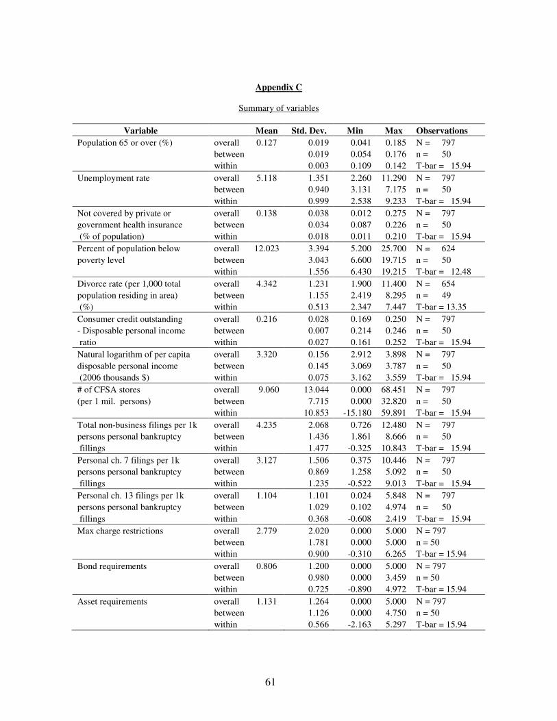
61

Appendix C

Summary of variables

Variable Mean Std. Dev. Min Max Observations

Population 65 or over (%) overall 0.127 0.019 0.041 0.185 N = 797

between 0.019 0.054 0.176 n = 50

within 0.003 0.109 0.142 T-bar = 15.94

Unemployment rate overall 5.118 1.351 2.260 11.290 N = 797

between 0.940 3.131 7.175 n = 50

within 0.999 2.538 9.233 T-bar = 15.94

Not covered by private or overall 0.138 0.038 0.012 0.275 N = 797

government health insurance between 0.034 0.087 0.226 n = 50

(% of population) within 0.018 0.011 0.210 T-bar = 15.94

Percent of population below overall 12.023 3.394 5.200 25.700 N = 624

poverty level between 3.043 6.600 19.715 n = 50

within 1.556 6.430 19.215 T-bar = 12.48

Divorce rate (per 1,000 total overall 4.342 1.231 1.900 11.400 N = 654

population residing in area) between 1.155 2.419 8.295 n = 49

(%) within 0.513 2.347 7.447 T-bar = 13.35

Consumer credit outstanding overall 0.216 0.028 0.169 0.250 N = 797

- Disposable personal income between 0.007 0.214 0.246 n = 50

ratio within 0.027 0.161 0.252 T-bar = 15.94

Natural logarithm of per capita overall 3.320 0.156 2.912 3.898 N = 797

disposable personal income between 0.145 3.069 3.787 n = 50

(2006 thousands $) within 0.075 3.162 3.559 T-bar = 15.94

# of CFSA stores overall 9.060 13.044 0.000 68.451 N = 797

(per 1 mil. persons) between 7.715 0.000 32.820 n = 50

within 10.853 -15.180 59.891 T-bar = 15.94

Total non-business filings per 1k overall 4.235 2.068 0.726 12.480 N = 797

persons personal bankruptcy between 1.436 1.861 8.666 n = 50

fillings within 1.477 -0.325 10.843 T-bar = 15.94

Personal ch. 7 filings per 1k overall 3.127 1.506 0.375 10.446 N = 797

persons personal bankruptcy between 0.869 1.258 5.092 n = 50

fillings within 1.235 -0.522 9.013 T-bar = 15.94

Personal ch. 13 filings per 1k overall 1.104 1.101 0.024 5.848 N = 797

persons personal bankruptcy between 1.029 0.102 4.974 n = 50

fillings within 0.368 -0.608 2.419 T-bar = 15.94

Max charge restrictions overall 2.779 2.020 0.000 5.000 N = 797

between 1.781 0.000 5.000 n = 50

within 0.900 -0.310 6.265 T-bar = 15.94

Bond requirements overall 0.806 1.200 0.000 5.000 N = 797

between 0.980 0.000 3.459 n = 50

within 0.725 -0.890 4.972 T-bar = 15.94

Asset requirements overall 1.131 1.264 0.000 5.000 N = 797

between 1.126 0.000 4.750 n = 50

within 0.566 -2.163 5.297 T-bar = 15.94

62

Appendix C (Continued)

Variable Mean Std. Dev. Min Max Observations

License related fees overall 1.573 0.909 0.000 5.000 N = 797

between 0.804 0.186 4.000 n = 50

within 0.414 -0.109 4.288 T-bar = 15.94

Rollovers restrictions overall 1.805 2.173 0.000 5.000 N = 797

between 1.657 0.000 5.000 n = 50

within 1.445 -1.695 6.491 T-bar = 15.94

Loan / check maximum amount overall 1.402 1.023 0.000 5.000 N = 797

between 0.786 0.000 3.250 n = 50

within 0.686 -0.179 4.736 T-bar = 15.94

63

Appendix D

Coding Criteria for the State Payday Lending Legislation Restriction Variables

Unless noted otherwise, each variable is coded between 0 (no restriction) and 5 (maximum restrictions); a smaller number means less restrictions. - the scale for each variable was constructed based on the actual distribution of outcomes, time and across state consistency being the decisive factor - if there was some change during the year, but not enough to move it another index category, I adjusted the previous figure by a small number (+/-0.1, depending on whether the change is less or more restrictive) - if there is a change during the year, the value for that year was a time weighted average of the new value and the previous year value The procedure is described in more details in chapter IV. A) Price restrictions - mainly fees limits - The cost of a first $300 (principal) 14-day loan if paid at maturity is

no cap [= 0] >45, but some cap [= 1.5] (30-45] [= 2.5] (15-30] [= 3.5] <15 [= 5]

- no explicit limit, but proposed max rates have to be approved [= 2.5] - after maturity, no more than usury charges or other limit [+ 0.5] - the calculated cost includes a non-recurring fee, like a set up initial customer account fee, that, if ignored, would move the cost of a first $300 loan to another category [+ 0.5]; [+ 1.0] if the non-recurring fee dominates - graduated rate /decreasing fee schedule in amount lent, if considering the whole range of the fee schedule, it will move it in another category [± 0.5] B) Licensing / entry restriction - mainly bond and net assets restrictions Bond requirements: - no bond [= 0.0] - bond instead of asset requirement for the same amount [= 0.1] - $1k -$5k [= 0.5] - $10k - $20k [= 1.5] - $25k [= 2.5] - not specified [= 2.5] - $50k [= 3.5] - $100k+ [= 4.5] - reduction in bond requirements for additional locations:

- additional bond 10% of the first license [- 0.50] - additional bond 20% of the first license [- 0.25] - additional bond 25% of the first license [- 0.20]

- capped for multiple licenses: - $ 25k [- 0.50] - $ 50k [- 0.25] - $150k [- 0.08] - $200k [- 0.06] - $300k [- 0.04] - $500k [- 0.03]

- the bond limit amount for multiple licenses has a maximum number of allowed locations / licenses: - up to 10 places of business under each multiple office license [+ 0.25]

64

- accepts letter of credit or interest-bearing assets instead of the bond [- 0.25] - must continue after the lender ceases operation, the renewal application is denied or the license is revoked:

- for 2 years [+ 0.2] - for 3 years [+ 0.3] - for 5 years [+ 0.5]

- the bond can be increased based on the volume of the applicant's business, on the financial condition of the licensee or the applicant for a license, or for violations. [+ 0.1] - continuous in nature [+ 0.1] Asset requirements:

liquid / readily

available assets

liquid assets can be

letter of credit

liquid assets

have to be cash

accepts line of credit

instead of the assets

require- ments are for

assets or capital

some reduction

for smaller city /

county size

(a) no restrictions [= 0.00] - - - - - -

(b) ≤$5k [= 0.00] [+ 0.05] [- 0.02] [+ 0.02] [- 0.03] [- 0.05] [- 0.05]

(c) ($5k - $10k] [= 0.00] [+ 0.05] [- 0.02] [+ 0.05] [- 0.05] [- 0.10] [- 0.05]

(d) ($10k - $20k] [= 0.50] [+ 0.10] [- 0.05] [+ 0.10] [- 0.10] [- 0.20] [- 0.10]

(e) $25k [= 1.00] [+ 0.25] [- 0.15] [+ 0.15] [- 0.25] [- 0.20] [- 0.20]

(f) $30k [= 1.25] [+ 0.25] [- 0.15] [+ 0.15] [- 0.25] [- 0.20] [- 0.20]

(g) $50k [= 2.00] [+ 0.50] [- 0.25] [+ 0.25] [- 0.50] [- 0.25] [- 0.25]

(h) $75k [= 2.50] [+ 0.50] [- 0.25] [+ 0.25] [- 0.50] [- 0.25] [- 0.25]

(i) $100k+ [= 3.00] [+ 0.50] [- 0.25] [+ 0.30] [- 0.50] [- 0.25] [- 0.25]

additional location requirements % of the

first location

17% 20% 25% 33%

continuous / maintained through the licensing

year rather than limited to an annual

basis

continuity requirement refer to

liquid assets

continuity requirement

does not refer to

liquid nor to net assets

(a) no restrictions

- - - - - - -

(b) ≤$5k [- 0.05] [- 0.04] [- 0.03] [- 0.02] [+ 0.05] [+ 0.05] [- 0.02]

(c) ($5k - $10k] [- 0.05] [- 0.04] [- 0.03] [- 0.02] [+ 0.10] [+ 0.05] [- 0.02]

(d) ($10k - $20k] [- 0.10] [- 0.09] [- 0.07] [- 0.05] [+ 0.15] [+ 0.10] [- 0.04]

(e) $25k [- 0.25] [- 0.23] [- 0.18] [- 0.13] [+ 0.25] [+ 0.15] [- 0.06]

(f) $30k [- 0.25] [- 0.23] [- 0.18] [- 0.13] [+ 0.30] [+ 0.15] [- 0.06]

(g) $50k [- 0.50] [- 0.45] [- 0.35] [- 0.25] [+ 0.50] [+ 0.25] [- 0.10]

(h) $75k [- 0.50] [- 0.45] [- 0.35] [- 0.25] [+ 0.75] [+ 0.25] [- 0.10]

(i) $100k+ [- 0.50] [- 0.45] [- 0.35] [- 0.25] [+ 1.00] [+ 0.25] [- 0.10]

- the asset requirement can be increased by the regulatory agency [+ 0.1]

65

- capped for multiple licenses: - $ 25k [- 0.50] - $ 50k [- 0.25] - $ 75k [- 0.17] - $ 220k [- 0.06] - $250k [- 0.05]

Initial / recurring license related fees: Licensing costs = application + license fees Let A denote the annual licensing costs, after the first year. To adjust for the fist year licensing costs, which could be different than the renewal annual licensing costs, let the “full” first two-year licensing costs (application + license fees) be denoted by F2y. If the licensing fees are not explicitly stated, but dollar limits are provided, and the rule for determining the fee is “to cover the cost of administering the law”, the upper limit was used. - no license fees [= 0] - annual licensing costs > 0 [= 0.5 + 0.002* A] - background check / fingerprint cards amount fee required, but not specified [+ 0.1]

- first year licensing costs are different than those in subsequent years: [+ 5

*22 AYF −

*0.002]

- licensing fees do not include the costs related to conducting the investigation into the application (for example, the costs of the publication of the notice of the filing of the application, the costs of the hearing), which are supposed to be billed separately upon the completion of the investigation, or pro rata share of all costs and expenses reasonably incurred in the administration of the law[+ 0.25] - licensing fees not explicitly stated, and there are no limits other than “to cover the cost of administering the law” [= 2.5] - renewal at more than 1 year intervals (2 years) [- 0.1] - fees for change of address, name, in control, or for the required registration of loan officers [+ 0.1] - annual volume fee [+ 0.25] - licensing fees reductions for multiple licenses:

additional locations licensing fees requirements % of the first location

annual licensing

costs for the first location

capped at up to 10

additional locations

0% 2% 10% 20-25% 40-50% >50%

(a) ≤$100 [- 0.01] [- 0.05] [- 0.04] [- 0.03] [- 0.02] [- 0.01] [- 0.01]

(b) ($100 - $250] [- 0.01] [- 0.15] [- 0.14] [- 0.12] [- 0.06] [- 0.02] [- 0.01]

(c) ($250 - $500] [- 0.05] [- 0.50] [- 0.49] [- 0.43] [- 0.31] [- 0.10] [- 0.05]

(d) ($500 - $1000] [- 0.07] [- 0.75] [- 0.72] [- 0.60] [- 0.38] [- 0.13] [- 0.07]

(e) ($1000 - $1500] [- 0.15] [- 1.25] [- 1.20] [- 1.00] [- 0.63] [- 0.30] [- 0.15]

(f) > $1500 [- 0.25] [- 1.50] [- 1.44] [- 1.20] [- 0.75] [- 0.35] [- 0.25]

- business examination costs (not included in the application or renewal fees) [+ 0.25] C) Business practice restrictions - lead to increases in the production costs Loan limitations: number of rollovers: - 0 [= 5] - 1 [= 4] - [2-3 times] [= 3] - (3-8) [= 2] - >8 (specified) [= 1] - not specified [= 0]

66

- allows renewals with no stated limit but only with charge restrictions - no extra charges allowed [= 4.5] - some extra charges allowed, but the restrictions dominate the charges that can be collected [= 4.3] - allows renewals beyond the stated limit if a distinct advantage to the borrower (for example, extension without any other charges)

- only one extra renewal with no extra charges [- 0.25] - unlimited renewals with no extra charges [- 0.50]

- time restriction - no rollover limits specified, but there are time charge restrictions

- interest can not be included into the principal [= 1] - maxim 12 weeks after the contract date [= 2]

- can renew beyond the stated rollover limit if maturity is increased to at least 28 days [- 0.50] - allows renewals beyond the stated limit within a given time, if the debtor has undergone recent consumer credit counseling [- 0.50]

- dollar limits on renewals (have to renew less than the original principal) - no rollover limits specified, but the principal has to be reduced 25% for a renewal [= 2] - the rollover limit is stated, but the principal has to be decreased

- by minimum 5% [+ 0.25] - by minimum 10% [+ 0.50]

- allows renewals beyond the stated limit if the principal is decreased by at least 10% [- 0.50] - allows renewals beyond the stated limit if the principal is increased by at least 10% [- 0.25]

- not allowed for a member of the military service [+ 0.25] - state wide common database [+ 0.25] Loan limitations: loan / check maximum amount - ≤$100 [= 5.0] - ($100-$300] [= 3.0] - ($300-$500] [= 2.5] - ($500-$1,500] [= 2.0] - >$1,500, but limit [= 1.0] - no limit [= 0.0] - no explicit limit is stated other than a reference to the borrower’s income [= 2.5] - if the stated limit amount includes the fees, and if considering the charges it would move it into a different category [+ 0.25] - amount is linked to the borrower’s income or ability to repay [+ 0.50] - have to check into a state wide common database [+ 0.25]

67

Appendix E

DID estimation: bankruptcy filings vs. payday lending stores

Dependent variables: personal filings per one thousands persons

(1) (2) (3) (4) (5) (6) (7) (8) (9)

total ch. 7 ch. 13 total ch. 7 ch. 13 total ch. 7 ch. 13

Lag of personal total filings 0.560 0.404 0.155 0.560 0.404 0.155 0.954 0.320 0.247

per 1k persons (7.51)** (6.16)** (7.37)** (10.27)** (7.09)** (5.93)** (60.44)** (10.23)** (14.86)**

Population 65 or over 17.780 19.033 -1.263 17.780 19.033 -1.263 0.969 7.119 -1.400

(%) (1.80) (2.15)* (0.32) (1.46) (1.29) (0.15) (0.86) (2.56)* (0.75)

Unemployment 0.167 0.052 0.114 0.167 0.052 0.114 0.168 0.063 0.064

rate (2.29)* (0.93) (3.24)** (1.82) (0.74) (2.38)* (4.60)** (1.75) (3.99)**

Lag of unemployment 0.089 0.104 -0.015 0.089 0.104 -0.015 -0.091 0.069 -0.005

rate (1.09) (1.48) (0.44) (1.14) (1.75) (0.36) (2.42)* (1.89) (0.30)

Not covered by health -0.550 1.051 -1.599 -0.550 1.051 -1.599 -1.512 -1.360 -0.230

insurance (% of population) (0.25) (0.54) (2.56)* (0.19) (0.40) (2.57)* (1.93) (1.85) (0.79)

Lag of not covered by health -0.624 -0.492 -0.131 -0.624 -0.492 -0.131 -0.569 -0.250 0.412

insurance (% of population) (0.34) (0.30) (0.18) (0.35) (0.25) (0.15) (0.70) (0.33) (1.06)

Consumer credit outstanding - Disposable 56.885 47.740 9.188

personal income ratio (.) (.) (.)

Lag of Consumer credit outstanding - Disposable -43.818 -38.672 -4.970

personal income ratio (1.58) (1.54) (0.34)

Divorce rate (per 1,000 total 0.107 0.059 0.049 0.107 0.059 0.049 0.037 0.090 0.001 population residing in area) (%) (1.31) (0.84) (1.64) (1.44) (0.79) (1.45) (0.95) (2.48)* (0.04)

Lag of divorce rate (per 1,000 total population residing -0.017 -0.119 0.102 -0.017 -0.119 0.102 0.018 0.022 0.045

in area) (%) (0.20) (1.58) (3.59)** (0.20) (1.55) (3.55)** (0.47) (0.60) (2.38)*

Ln of per capita real -1.222 -0.401 -0.825 -1.222 -0.401 -0.825 -0.866 -0.154 -0.211

disposable personal income (0.79) (0.29) (1.36) (0.68) (0.23) (1.29) (1.17) (0.29) (0.66)

67

68

Appendix E (Continued)

(1) (2) (3) (4) (5) (6) (7) (8) (9)

total ch. 7 ch. 13 total ch. 7 ch. 13 total ch. 7 ch. 13

Lag of ln of per capita real 0.031 -1.036 1.048 0.031 -1.036 1.048 0.382 -0.604 -0.217

disposable personal income (0.02) (0.79) (1.73) (0.02) (0.61) (1.56) (0.52) (1.14) (0.68)

Stores -0.005 -0.002 -0.003 -0.005 -0.002 -0.003 -0.005 0.002 0.003

(0.54) (0.22) (1.39) (0.50) (0.20) (0.80) (2.40)* (0.74) (1.72)

Stores*Change 0.003 -0.001 0.003 0.003 -0.001 0.003 0.002 -0.009 0.003

(0.31) (0.10) (1.23) (0.28) (0.09) (0.71) (0.91) (2.10)* (1.46)

Change 0.000 0.000 0.000 0.000 0.000 0.000 -0.062 -0.075 0.072

(.) (.) (.) (.) (.) (.) (1.42) (0.77) (1.05)

2005 dummy 2.949 2.689 0.274 1.703 1.754 -0.050 1.699 2.878 -0.129

(6.19)** (6.19)** (1.76) (10.35)** (11.95)** (0.81) (13.32)** (15.06)** (1.25)

2006 dummy -2.882 -2.469 -0.397 -3.836 -3.157 -0.676 -4.445 -1.990 -0.935 (5.46)** (5.21)** (2.19)* (18.28)** (18.56)** (6.13)** (30.77)** (8.77)** (7.62)**

Constant 1.477 2.798 -1.253 -0.548 1.457 -1.977 1.469 2.050 0.903

(0.31) (0.68) (0.71) (0.08) (0.26) (0.59) (2.38)* (1.52) (0.89)

Observations 561 561 561 561 561 561 560 560 560

Number of states 48 48 48 48 48 48 47 47 47

R-squared 0.87 0.86 0.53 0.87 0.86 0.53

State fixed effects Y Y Y Y Y Y N N N

Year fixed effects Y Y Y Y Y Y Y Y Y

* significant at 5%; ** significant at 1%

(1) - (3) Robust t statistics in parentheses

(4) - (6) bootstrapped SE - z statistics in parentheses

(7) - (9) FGLS to correct for autocorrelation & heteroskedasticity - z statistics in parentheses

68

69

Appendix F

DID estimation: bankruptcy filings vs. payday lending stores (divorce rate omitted)

Dependent variables: personal filings per one thousands persons

(1) (2) (3) (4) (5) (6) (7) (8) (9)

total ch. 7 ch. 13 total ch. 7 ch. 13 total ch. 7 ch. 13

Lag of personal total filings 0.628 0.441 0.186 0.628 0.441 0.186 0.953 0.383 0.203

per 1k persons (9.45)** (7.75)** (9.60)** (13.09)** (9.14)** (6.39)** (80.31)** (17.12)** (15.08)**

Population 65 or over 5.171 8.691 -3.596 5.171 8.691 -3.596 0.351 6.888 -2.663

(%) (0.72) (1.40) (1.13) (0.61) (0.83) (0.51) (0.38) (4.41)** (1.76)

Unemployment 0.148 0.068 0.078 0.148 0.068 0.078 0.065 0.070 0.038

rate (3.47)** (1.68) (4.22)** (2.29)* (0.96) (2.03)* (4.72)** (3.63)** (3.51)**

Not covered by health -0.442 1.217 -1.640 -0.442 1.217 -1.640 -1.026 0.008 -0.294

insurance (% of population) (0.29) (0.93) (2.92)** (0.22) (0.70) (2.28)* (2.55)* (0.02) (1.07)

Consumer credit outstanding – Disposable personal 0.000 0.000 0.000 9.689 10.236 -0.394

income ratio (.) (.) (.) (.) (.) (.)

Ln of per capita real -0.529 -0.900 0.353 -0.529 -0.900 0.353 -0.156 -0.126 -0.304

disposable personal income (0.54) (1.03) (0.80) (0.43) (0.82) (0.40) (1.28) (0.52) (1.52)

Stores -0.001 0.002 -0.003 -0.001 0.002 -0.003 -0.002 0.008 0.003

(0.13) (0.28) (1.55) (0.18) (0.33) (0.88) (0.87) (2.60)** (1.96)

Stores*Change 0.002 -0.003 0.005 0.002 -0.003 0.005 0.002 -0.005 0.003

(0.32) (0.47) (2.49)* (0.50) (0.55) (1.45) (0.86) (1.63) (1.70)

Change 0.000 0.000 0.000 0.000 0.000 0.000 -0.003 0.012 0.003

(.) (.) (.) (.) (.) (.) (0.07) (0.20) (0.06)

2005 dummy 2.447 2.507 -0.050 1.800 1.823 -0.023 1.416 2.406 -0.128

(7.09)** (7.97)** (0.37) (15.49)** (18.71)** (0.71) (15.72)** (19.33)** (1.60)

2006 dummy -3.494 -2.675 -0.807 -4.098 -3.313 -0.782 -4.722 -2.561 -0.880

(8.39)** (7.24)** (4.43)** (20.21)** (18.34)** (7.70)** (46.08)** (16.99)** (9.24)**

Constant 1.658 2.328 -0.601 -0.094 0.478 -0.530 0.680 0.354 1.158

(0.51) (0.80) (0.39) (0.02) (0.12) (0.18) (1.44) (0.39) (1.58)

69

70

Appendix F (Continued)

(1) (2) (3) (4) (5) (6) (7) (8) (9)

total ch. 7 ch. 13 total ch. 7 ch. 13 total ch. 7 ch. 13

Observations 745 745 745 745 745 745 745 745 745

Number of states 50 50 50 50 50 50 50 50 50

R-squared 0.88 0.86 0.57 0.88 0.86 0.57

State fixed effects Y Y Y Y Y Y N N N

Year fixed effects Y Y Y Y Y Y Y Y Y

* significant at 5%; ** significant at 1%

(1) - (3) Robust t statistics in parentheses

(4) - (6) bootstrapped SE – z statistics in parentheses

(7) - (9) FGLS to correct for autocorrelation & heteroskedasticity - z statistics in parentheses

70

71

Appendix G

Akaike Information Criterion (AIC) optimal lag structure

(1) (2) (3) (4) (5) (6)

# of

years

with

payday

stores

st

total

total

filings per 1k

persons

personal

ch. 7

filings

per 1k persons

personal

ch. 13

filings per 1k

persons

Stores (per 1 mil.

persons)

(1) (2) (3) (4) (5) (6)

13 AL 4 4 2 4 10 NE 0 0 3 3

2 AK 3 2 1 8 NV 0 0 4 1

17 AZ 0 0 2 2 7 NH 0 0 1 1

8 AR 2 2 1 1 0 NJ 0 0 2

10 CA 4 4 4 2 17 NM 0 3 2 4

6 CO 0 NY 0 0 2

0 CT 4 0 2 13 NC 4 4 2 1

8 DE 1 0 2 1 6 ND 2 2 1 4

8 DC 4 4 4 3 17 OH 4 4 4 3

12 FL 1 1 3 3 17 OK 4 4 2 1

14 GA 4 4 2 1 9 OR 4 4 1 3

10 HI 4 1 0 3 17 PA 4 4 2 1

9 ID 4 4 1 4 6 RI 0 0 1

12 IL 4 4 2 1 13 SC 2 4 2 1

14 IN 4 4 1 1 5 SD 2 2 1 4

10 IA 0 0 0 1 17 TN 0 4 2 1

17 KS 4 4 1 1 17 UT 1 3 2 2

16 KY 4 4 4 1 0 VT 4 4 2

17 LA 4 2 2 1 17 VA 0 0 2 2

3 ME 4 4 3 17 WA 0 0 2 1

17 MD 1 0 2 1 0 WV 4 4 1 4

0 MA 0 0 2 17 WI 4 4 2 1

9 MI 4 4 4 1 9 WY 0 2 2 2

0 MN 4 4 3 all states 4 4 2 4

11 MS 1 3 2 1 all states* 4 4 2 4

17 MO 4 4 2 1 * with other variables included

8 MT 4 2 2 4

71

72

Appendix H

Summary of Granger causality between personal total bankruptcy filings and payday lending stores

Specification # of lags

Time FE

Other variables included in the bankruptcy eq.

Other variables included in the bankruptcy eq.

Ho: coef. on Stores are jointly = 0

Ho: coef. on bankruptcy are

jointly = 0 Conclusion

OLS + FE + robust st. errors 4 y note 1 note 2 fail to reject reject b => s

OLS + FE + bootstrapped st. errors 4 y note 1 note 2 fail to reject fail to reject b <=> s

FGLS + panel-specific AR1 autocorrelation structure + heteroskedastic error structure

4 y note 1 note 2 reject reject b ≠ s

OLS + FE + robust st. errors 4 n note 1 note 2 fail to reject reject b => s

OLS + FE + bootstrapped st. errors 4 n note 1 note 2 fail to reject fail to reject b <=> s

FGLS + panel-specific AR1 autocorrelation structure + heteroskedastic error structure

4 n note 1 note 2 fail to reject reject b => s

OLS + FE + robust st. errors 1 y note 1 note 2 fail to reject reject b => s

OLS + FE + bootstrapped st. errors 1 y note 1 note 2 fail to reject reject b => s

FGLS + panel-specific AR1 autocorrelation structure + heteroskedastic error structure

1 y note 1 note 2 fail to reject reject b => s

OLS + FE + robust st. errors 1 y note 3 note 4 fail to reject reject b => s

OLS + FE + bootstrapped st. errors 1 y note 3 note 4 fail to reject fail to reject b <=> s

FGLS + panel-specific AR1 autocorrelation structure + heteroskedastic error structure

1 y note 3 note 4 fail to reject reject b => s

OLS + FE + robust st. errors 1 n note 1 note 2 fail to reject reject b => s

OLS + FE + bootstrapped st. errors 1 n note 1 note 2 fail to reject reject b => s

FGLS + panel-specific AR1 autocorrelation structure + heteroskedastic error structure

1 n note 1 note 2 fail to reject reject b => s

OLS + FE + robust st. errors 1 n note 3 note 4 fail to reject reject b => s

OLS + FE + bootstrapped st. errors 1 n note 3 note 4 fail to reject reject b => s

FGLS + panel-specific AR1 autocorrelation structure + heteroskedastic error structure

1 n note 3 note 4 fail to reject reject b => s

72

73

Appendix H (Continued)

note 1: unemployment rate, population 65 or over (%), not covered by health insurance (% of population), natural logarithm of per capita disposable personal income (2006 thousands $) (denoted in this table as income) note 3: unemployment rate

note 2: income + legislative variables (max charge restrictions, bond requirements, asset requirements, license related fees, rollovers restrictions, loan / check maximum amount) note 4: the legislative variables in note 2

b => s bankruptcy "causes" payday stores ; b <=> s bi-directional causality ; b ≠ s no causal relationship

73

74

Appendix I

Summary of Granger causality between personal ch. 7 bankruptcy filings and payday lending stores

Specification # of lags

Time FE

Other variables included in the bankruptcy eq.

Other variables included in the bankruptcy eq.

Ho: coef. on Stores are jointly = 0

Ho: coef. on bankruptcy are

jointly = 0 Conclusion

OLS + FE + robust st. errors 4 y note 1 note 2 fail to reject reject b => s

OLS + FE + bootstrapped st. errors 4 y note 1 note 2 fail to reject fail to reject b <=> s

FGLS + panel-specific AR1 autocorrelation structure + heteroskedastic error structure

4 y note 1 note 2 fail to reject reject b => s

OLS + FE + robust st. errors 4 n note 1 note 2 fail to reject reject b => s

OLS + FE + bootstrapped st. errors 4 n note 1 note 2 fail to reject fail to reject b <=> s

FGLS + panel-specific AR1 autocorrelation structure + heteroskedastic error structure

4 n note 1 note 2 fail to reject reject b => s

OLS + FE + robust st. errors 1 y note 1 note 2 fail to reject reject b => s

OLS + FE + bootstrapped st. errors 1 y note 1 note 2 fail to reject reject b => s

FGLS + panel-specific AR1 autocorrelation structure + heteroskedastic error structure

1 y note 1 note 2 fail to reject reject b => s

OLS + FE + robust st. errors 1 y note 3 note 4 fail to reject reject b => s

OLS + FE + bootstrapped st. errors 1 y note 3 note 4 fail to reject fail to reject b <=> s

FGLS + panel-specific AR1 autocorrelation structure + heteroskedastic error structure

1 y note 3 note 4 fail to reject reject b => s

OLS + FE + robust st. errors 1 n note 1 note 2 fail to reject fail to reject b <=> s

OLS + FE + bootstrapped st. errors 1 n note 1 note 2 fail to reject fail to reject b <=> s

FGLS + panel-specific AR1 autocorrelation structure + heteroskedastic error structure

1 n note 1 note 2 fail to reject reject b => s

OLS + FE + robust st. errors 1 n note 3 note 4 fail to reject reject b => s

OLS + FE + bootstrapped st. errors 1 n note 3 note 4 reject reject b ≠ s

FGLS + panel-specific AR1 autocorrelation structure + heteroskedastic error structure

1 n note 3 note 4 fail to reject reject b => s

74

75

Appendix I (Continued)

note 1: unemployment rate, population 65 or over (%), not covered by health insurance (% of population), natural logarithm of per capita disposable personal income (2006 thousands $) (denoted in this table as income) note 3: unemployment rate

note 2: income + legislative variables (max charge restrictions, bond requirements, asset requirements, license related fees, rollovers restrictions, loan / check maximum amount) note 4: the legislative variables in note 2

b => s bankruptcy "causes" payday stores ; b <=> s bi-directional causality ; b ≠ s no causal relationship

75

76

Appendix J

Summary of Granger causality between personal ch. 13 bankruptcy filings and payday lending stores

Specification # of lags

Time FE

Other variables included in the bankruptcy eq.

Other variables included in the bankruptcy eq.

Ho: coef. on Stores are jointly = 0

Ho: coef. on bankruptcy are

jointly = 0 Conclusion

OLS + FE + robust st. errors 2 y note 1 note 2 reject fail to reject s => b

OLS + FE + bootstrapped st. errors 2 y note 1 note 2 fail to reject fail to reject b <=> s

FGLS + panel-specific AR1 autocorrelation structure + heteroskedastic error structure

2 y note 1 note 2 reject fail to reject s => b

OLS + FE + robust st. errors 2 n note 1 note 2 fail to reject reject b => s

OLS + FE + bootstrapped st. errors 2 n note 1 note 2 fail to reject fail to reject b <=> s

FGLS + panel-specific AR1 autocorrelation structure + heteroskedastic error structure

2 n note 1 note 2 fail to reject reject b => s

OLS + FE + robust st. errors 1 y note 1 note 2 fail to reject fail to reject b <=> s

OLS + FE + bootstrapped st. errors 1 y note 1 note 2 fail to reject fail to reject b <=> s

FGLS + panel-specific AR1 autocorrelation structure + heteroskedastic error structure

1 y note 1 note 2 fail to reject fail to reject b <=> s

OLS + FE + robust st. errors 1 y note 3 note 4 fail to reject fail to reject b <=> s

OLS + FE + bootstrapped st. errors 1 y note 3 note 4 fail to reject fail to reject b <=> s

FGLS + panel-specific AR1 autocorrelation structure + heteroskedastic error structure

1 y note 3 note 4 fail to reject fail to reject b <=> s

OLS + FE + robust st. errors 1 n note 1 note 2 fail to reject reject b => s

OLS + FE + bootstrapped st. errors 1 n note 1 note 2 fail to reject fail to reject b <=> s

FGLS + panel-specific AR1 autocorrelation structure + heteroskedastic error structure

1 n note 1 note 2 fail to reject fail to reject b <=> s

OLS + FE + robust st. errors 1 n note 3 note 4 fail to reject reject b => s

OLS + FE + bootstrapped st. errors 1 n note 3 note 4 fail to reject reject b => s

FGLS + panel-specific AR1 autocorrelation structure + heteroskedastic error structure

1 n note 3 note 4 reject fail to reject s => b

76

77

Appendix J (Continued) note 1: unemployment rate, population 65 or over (%), not covered by health insurance (% of population), natural logarithm of per capita disposable personal income (2006 thousands $) (denoted in this table as income) note 3: unemployment rate

note 2: income + legislative variables (max charge restrictions, bond requirements, asset requirements, license related fees, rollovers restrictions, loan / check maximum amount) note 4: the legislative variables in note 2

b => s bankruptcy "causes" payday stores ; b <=> s bi-directional causality ; b ≠ s no causal relationship

77

78

Appendix K

Granger causality test between payday lending stores and personal bankruptcy filings (AIC lag structure)

(1) (2) (3) (4) (5) (6)

total Stores ch. 7 Stores ch. 13 Stores

L1. Personal total filings per 1k persons 0.747 0.227

(12.49)** (0.99)

L2. Personal total filings per 1k persons 0.378 0.399

(3.74)** (0.91)

L3. Personal total filings per 1k persons -0.317 0.262

(3.00)** (0.55)

L4. Personal total filings per 1k persons 0.149 -0.682

(2.17)* (2.32)*

L1. Personal ch. 7 filings per 1k persons 0.455 0.384 (7.28)** (1.46)

L2. Personal ch. 7 filings per 1k persons 0.81 -0.072

(7.75)** (0.15)

L3. Personal ch. 7 filings per 1k persons -0.429 0.871

(3.69)** (1.57)

L4. Personal ch. 7 filings per 1k persons 0.11 -0.918

(1.42) (2.56)*

L1. Personal ch. 13 filings per 1k persons 1.423 -1.522

(35.81)** (2.05)*

L2. Personal ch. 13 filings per 1k persons -0.481 4.828

(11.90)** (3.53)**

L3. Personal ch. 13 filings per 1k persons -3.36

(2.57)*

L4. Personal ch. 13 filings per 1k persons 0.222

(0.29)

L1. Stores 0.012 1.301 0.003 1.298 0.004 1.319

(2.40)* (28.07)** (0.65) (27.87)** (3.12)** (31.04)**

78

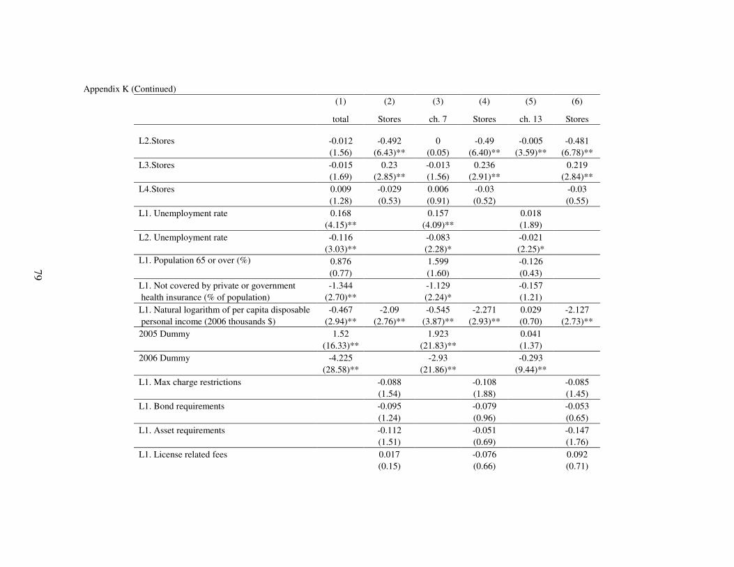
79

Appendix K (Continued)

(1) (2) (3) (4) (5) (6)

total Stores ch. 7 Stores ch. 13 Stores

L2.Stores -0.012 -0.492 0 -0.49 -0.005 -0.481

(1.56) (6.43)** (0.05) (6.40)** (3.59)** (6.78)**

L3.Stores -0.015 0.23 -0.013 0.236 0.219

(1.69) (2.85)** (1.56) (2.91)** (2.84)**

L4.Stores 0.009 -0.029 0.006 -0.03 -0.03

(1.28) (0.53) (0.91) (0.52) (0.55)

L1. Unemployment rate 0.168 0.157 0.018

(4.15)** (4.09)** (1.89)

L2. Unemployment rate -0.116 -0.083 -0.021

(3.03)** (2.28)* (2.25)*

L1. Population 65 or over (%) 0.876 1.599 -0.126

(0.77) (1.60) (0.43)

L1. Not covered by private or government -1.344 -1.129 -0.157

health insurance (% of population) (2.70)** (2.24)* (1.21)

L1. Natural logarithm of per capita disposable -0.467 -2.09 -0.545 -2.271 0.029 -2.127

personal income (2006 thousands $) (2.94)** (2.76)** (3.87)** (2.93)** (0.70) (2.73)**

2005 Dummy 1.52 1.923 0.041

(16.33)** (21.83)** (1.37)

2006 Dummy -4.225 -2.93 -0.293

(28.58)** (21.86)** (9.44)**

L1. Max charge restrictions -0.088 -0.108 -0.085

(1.54) (1.88) (1.45)

L1. Bond requirements -0.095 -0.079 -0.053

(1.24) (0.96) (0.65)

L1. Asset requirements -0.112 -0.051 -0.147

(1.51) (0.69) (1.76)

L1. License related fees 0.017 -0.076 0.092

(0.15) (0.66) (0.71)

79

80

Appendix K (Continued)

(1) (2) (3) (4) (5) (6)

total Stores ch. 7 Stores ch. 13 Stores

L1. Rollovers restrictions 0.02 0.011 0.038

(0.43) (0.24) (0.81)

L1. Loan / check maximum amount 0.167 0.169 0.008

(1.48) (1.44) (0.07)

Constant 1.693 7.832 1.321 7.127 -0.067 8.375

(2.69)** (2.93)** (2.41)* (2.55)* (0.44) (3.20)**

Observations 590 590 590 590 693 590

Number of states 50 50 50 50 50 50

Time effects Y Y Y Y Y Y

All equations estimated by FGLS to correct for autocorrelation & heteroskedasticity - z statistics in parentheses

* significant at 5%; ** significant at 1% L1. in front of a variable X means the first lag of X, L2. in front of a variable X means the second lag of X, and so on

Specifications should be interpreted in pairs: (1) & (2), (3) & (4), and (5) & (6)

80

81

Appendix L

Granger causality test between payday lending stores and personal bankruptcy filings (parsimonious lag structure)

(1) (2) (3) (4) (5) (6)

total Stores ch. 7 Stores ch. 13 Stores

L1. Personal total filings per 1k persons 0.955 0.272

(84.14)** (3.60)**

L1. Personal ch. 7 filings per 1k persons 0.916 0.398

(62.33)** (3.79)**

L1. Personal ch. 13 filings per 1k persons 0.944 0.161

(69.72)** (1.37)

L1. Stores (per 1 mil. persons) -0.002 1.032 -0.001 1.035 0 1.047

(1.05) (68.98)** (0.95) (70.54)** (0.35) (72.55)**

L1. Unemployment rate 0.022 0.03 -0.006

(1.81) (3.01)** (0.92)

2005 Dummy 1.293 1.544 -0.14

(17.18)** (23.96)** (4.82)**

2006 Dummy -4.877 -4.283 -0.504

(56.49)** (54.07)** (16.45)**

L1. Max charge restrictions -0.091 -0.103 -0.107

(1.82) (2.06)* (2.10)*

L1. Bond requirements -0.073 -0.049 -0.104

(0.93) (0.61) (1.25)

L1. Asset requirements -0.147 -0.104 -0.197

(1.96) (1.37) (2.56)*

L1. License related fees 0.083 0.004 0.089

(0.75) (0.04) (0.76)

L1. Rollovers restrictions 0.055 0.047 0.044

(1.14) (0.97) (0.90)

L1. Loan / check maximum amount 0.13 0.125 0.069

(1.17) (1.13) (0.59)

81

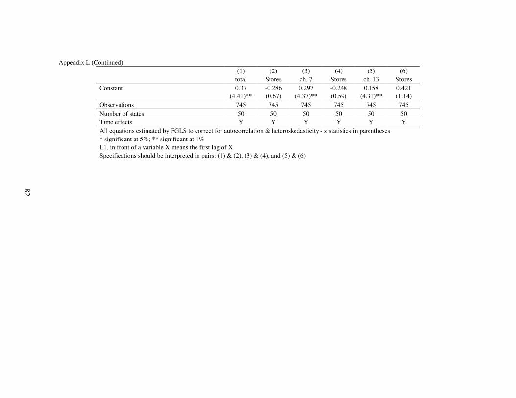
82

Appendix L (Continued)

(1) (2) (3) (4) (5) (6)

total Stores ch. 7 Stores ch. 13 Stores

Constant 0.37 -0.286 0.297 -0.248 0.158 0.421

(4.41)** (0.67) (4.37)** (0.59) (4.31)** (1.14)

Observations 745 745 745 745 745 745

Number of states 50 50 50 50 50 50

Time effects Y Y Y Y Y Y

All equations estimated by FGLS to correct for autocorrelation & heteroskedasticity - z statistics in parentheses

* significant at 5%; ** significant at 1%

L1. in front of a variable X means the first lag of X

Specifications should be interpreted in pairs: (1) & (2), (3) & (4), and (5) & (6)

82

83

REFERENCES

Agarwal, Sumit and Liu, Chunlin, “Determinants of credit card delinquency and bankruptcy: Macroeconomic factors”, Journal of Economics and Finance, Vol. 27, No. 1 (March, 2003), pp. 75-84

Barth, James R.; Cordes, Joseph J.; and Yezer, Anthony M. J. , “Benefits and Costs of

Legal Restrictions on Personal Loan Markets”, Journal of Law and Economics, Vol. 29, No. 2. (Oct., 1986), pp. 357-380.

Brooks, Richard R.W., “Credit past due”, Columbia Law Review, Vol. 106,

No. 4 (2006), pp. 994-1028 Buckley, F. H.; Brinig, Margaret F., “The Bankruptcy Puzzle”, The Journal of Legal

Studies, Vol. 27, No. 1. (Jan., 1998), pp. 187-207. Burkey, Mark L. and Simkins, Scott P., “Factors Affecting the Location of Payday

Lending and Traditional Banking Services in North Carolina” Review of Regional

Studies, Vol. 34, No. 2 (Fall 2004), pp. 191-205 Chessin, Paul, “Borrowing from Peter to pay Paul: A statistical analysis of Colorado's

Deferred Deposit Loan Act”, Denver University Law Review, Vol. 83 (2005), pp. 387-423

Domowitz, Ian; Sartain, Robert L., “Determinants of the Consumer Bankruptcy

Decision”, The Journal of Finance, Vol. 54, No. 1. (Feb., 1999), pp. 403-420. Domowitz, Ian; Eovaldi, Thomas L., “The Impact of the Bankruptcy Reform Act of 1978

on Consumer Bankruptcy”, Journal of Law and Economics, Vol. 36, No. 2. (Oct., 1993), pp. 803-835.

Elliehausen, Gregory and Lawrence, Edward C. , “Payday Advance Credit in America:

an Analysis of Customer Demand”, (Monograph No. 35). Washington, DC: Georgetown University, McDonough School of

Business, Credit Research Center (Apr. 2001) Fay, S., Hurst, E. and White, M.J., “The Household Bankruptcy Decision”, The American

Economic Review, Vol. 92, No. 3. (Jun., 2002), pp. 706-718. Flannery, Mark and Samolyk, Katherine, “Payday Lending: Do the Costs Justify the

Price?” FDIC Center for Financial Research Working Paper No. 2005-09, Jun. 2005

84

Granger, C.W.J., "Investigating Causal Relations by Econometric Models and Cross-spectral Methods", Econometrica, Vol. 37, No. 3 (Aug. 1969), pp. 424-438

Graves, Steven M., “Landscapes of predation, landscapes of neglect: A location analysis

of payday lenders and banks”, Professional Geographer, Vol. 55, Iss. 3 (2003), pp. 303-317

Graves, Steven M. and Peterson, Christopher Lewis, “Predatory Lending and the

Military: The Law and Geograpy of 'Payday' Loans in Military Towns” Ohio

State Law Journal, Vol. 66, p. 653 (2005) Gropp, Reint; Scholz, John Karl; White, Michelle J., “Personal Bankruptcy and Credit

Supply and Demand”, The Quarterly Journal of Economics, Vol. 112, No. 1. (Feb., 1997), pp. 217-251.

Gross, David B.; Souleles, Nicholas S., “An Empirical Analysis of Personal Bankruptcy

and Delinquency”, The Review of Financial Studies, Vol. 15, No. 1. (Spring, 2002), pp. 319-347.

Himmelstein David U., Warren E, Thorne D, and Woolhandler S., “Illness and injury as

contributors to bankruptcy”, Health Affairs, Vol. 24, Iss. 2, (2005), pp. W563-W573

Huckstep, Aaron, “Payday Lending: Do Outrageous Prices Necessarily Mean Outrageous

Profits?”, Fordham Journal of Corporate & Financial Law, Vol. XII, No. 1 (Oct. 2006), pp. 203-232

Johnson, Creola, “Payday loans: Shrewd business or predatory lending?”, Minnesota

Law Review, Vol. 87, Iss. 1 (2002), pp. 1-152 Karlan, Dean and Zinman, Jonathan, “Expanding Credit Access: Using Randomized

Supply Decisions to Estimate the Impacts”, Working paper, Nov. 2007; available at http://www.dartmouth.edu/~jzinman/ (accessed 12/7/2007)

Laibson, David. "Golden Eggs and Hyperbolic Discounting." The Quarterly Journal of

Economics, Vol. 112, Iss. 2, (1997), 443-77 Luckett, Charles A., “Personal bankruptcies”, Federal Reserve Bulletin, 1988,

pp. 591-603 Mann, Ronald J. and Hawkins, Jim, “Just until payday”, UCLA Law Review, Vol. 54,

Iss. 4 (2007), pp. 855-912

85

Melzer, Brian, The Real Costs of Credit Access: Evidence from the Payday Lending

Market, Job market paper, PhD Candidate in Economics, (Expected graduation June 2008), Graduate School of Business, University of Chicago; available at http://home.uchicago.edu/~bmelzer/ (accessed 2/19/2008)

Morgan, Donald P., “Defining and Detecting Predatory Lending”, Federal Reserve Bank

of New York, Staff Report no. 273 (Jan. 2007) Morgan, Donald P. and Strain, Michael R., “Payday Holiday: How Households Fare after

Payday Credit Bans”, Federal Reserve Bank of New York Staff Reports, no. 309, Nov. 2007

Morgan, Donald P. and Strain, Michael R., “Payday Holiday: How Households Fare after

Payday Credit Bans”, Federal Reserve Bank of New York, Staff Report no. 309

(November 2007) Morse, Adair, “Payday Lenders: Heroes or Villains?”, Working paper, Jan. 2007,

Graduate School of Business, University of Chicago; Available at http://faculty.chicagogsb.edu/adair.morse/ (accessed 12/7/2007)

Posner, Eric A., “Contract Law in the Welfare State: A Defense of the Unconscionability

Doctrine, Usury Laws, and Related Limitations on the Freedom to Contract , The

Journal of Legal Studies, Vol. 24, No. 2. (Jun., 1995), pp. 283-319 Skiba, Paige M. and Tobacman, Jeremy, “Measuring the Individual-Level Effects of

Access to Credit: Evidence from Payday Loans”, Ph.D. Job Market Paper, (Jan. 2007) for Skiba, Department of Economics, University of California

Snarr, Robert W. Jr., “No Cash ‘til Payday: The Payday Lending Industry”, Compliance

Corner, Federal Reserve Bank of Philadelphia, 1st Quarter 2002 Stegman, Michael A., “Payday Lending”, The Journal of Economic Perspectives,

Volume 21, Number 1, Winter 2007 Stegman, Michael A. and Faris, R. “Payday Lending: A Business Model that Encourages

Chronic Borrowing” Economic Development Quarterly, Vol. 17, No. 1, 8-32 (2003)

Strotz, Robert H., "Myopia and Inconsistency in Dynamic Utility Maximization," The

Review of Economic Studies, Vol. XXIII (1956), 165-80 The Washington State Department of Financial Institutions, "2006 Payday Lending

Report", Available at http://www.dfi.wa.gov/cs/check.htm#payday_reports (accessed 3/28/2008)

86

White, Michelle J., “Why Don't More Households File for Bankruptcy?”, The Journal of

Law, Economics, and Organization, Vol. 14, No. 2 (October 1998), pp. 205-31 Wilson, Bart J., Findlay, David W., Meehan, James W. , Wellford, Charissa P. and

Schurter, Karl , “An Experimental Analysis of the Demand for Payday Loans”, working paper (2008) Available at SSRN: http://ssrn.com/abstract=1083796