RESTORATION OF VARIABLE DENSITY FILM SOUNDTRACKS

A. Hassaıne1, E. Decenciere1 and B. Besserer2

1 Centre de Morphologie MathematiqueEcole Nationale Superieure des Mines de Paris77305 Fontainebleau, France{hassaine,decencie}@cmm.ensmp.fr

2 Laboratoire Informatique, Image, InteractionUniversite de La Rochelle17042 La Rochelle, Francebernard.besserer@univ-lr.fr

ABSTRACTThe restoration of motion picture films has been an active re-search field for many years. The restoration of the soundtrackhowever has mainly been performed at the audio domain inspite of the fast that it is recorded as a continuous image onthe film stock.

In this paper, we propose a new restoration method forvariable density soundtracks. The method first detects andcorrects accurately the azimuth deviation. A robust thresh-olding technique based on the minimization of the total vari-ation is then performed to remove the remaining faults.

Restoration results are very promising and testify to theefficiency of our method.

1. INTRODUCTION

Most film stocks produced since the Thirties use an opticalsoundtrack to record the sound. According to the standard“Academy Optical Mono track” which was introduced by“The Academy of Motion Picture Arts and Sciences”, theoptical soundtrack is located in a space of 3 mm between theimages of the film and the perforations. Therefore, dupli-cating a film makes it possible to duplicate its soundtrack atthe same time. Two types of optical soundtracks exist: vari-able area soundtracks which contain a bright region locatedbetween two dark regions; the length of the bright regionis directly proportional to the amplitude of the audio signal.And density variable soundtracks for which the brightness ofthe soundtrack, at each instant, is directly proportional to thesignal audio amplitude (fig. 1).

Figure 1: From left to right: variable density soundtrack,variable area soundtrack.

When the film is read, the soundtrack is lighted with alamp through a narrow slit. The light intensity which goes

through the soundtrack is measured and transformed to anelectric signal by a photodetector. This signal is then con-verted to sound via a classical amplification chain (fig. 2).Note that this process is used for both variable area and vari-able density soundtracks.

Exiter lamp

Slit

Optical soundtrack

Photodetector

Electrical signal

Figure 2: The process of reading a soundtrack.

Nowadays, optical recorders have a bandwidth of 20Hzto 14 kHz. The spatial resolution of the film stock usedfor optical soundtracks is about 100 lines per mm. Sincea 35mm film travels at 456mm per second, the maximum“bandwidth” of the film itself as analog optical carrier doesnot exceed 22 kHz.

The defiler used in this work contains a linear cameraable to scan 48000 lines of 512 pixel per second with a res-olution of 3200 DPI and a gray level depth of 8 bits (fig. 3).This resolution is good enough for processing high frequen-cies (it meets the requirements of the “X”-curve [2]). Forpractical reasons, an image is saved each time 640 lines arecaptured. Therefore, we deal with images which are 512 pix-els wide and 640 pixels high.

Unfortunately, the optical soundtrack undergoes thesame type of degradations as the images of the film (dust,scratches, ...etc). Moreover, since the soundtrack is close tothe extremity of the film, it is sometimes degraded by abra-sion or altered over a large surface due to moisture. Thesoundtrack might also be badly exposed. This problem isdue to the diffusion of light during different duplication pro-cesses.

In most cases, the restoration of the soundtrack is per-formed in the sound domain, using signal processing meth-ods, in spite of the fact that it is recorded as a continuous

17th European Signal Processing Conference (EUSIPCO 2009) Glasgow, Scotland, August 24-28, 2009

© EURASIP, 2009 2589

Figure 3: The scanner used in our work.

image between the film images and the perforations. Work-ing with the image representation of the soundtrack has sev-eral advantages. First, the defects are visible at the imagelevel. Most importantly, an image-based restoration makes itpossible to preserve the authentic sound as it was originallyrecorded, whereas an audio-based restoration might causethe loss of this authenticity (by filtering a noise which wasoriginally present in the sound for instance).

This work is undertaken within the “Resonances” projectwhich was launched in 2005 and aims to propose an auto-matic restoration method for optical soundtracks. We pro-posed in [3] a restoration method for variable area sound-tracks at the image level which gives generally good results.In this paper, we propose a new method for the restoration ofvariable density soundtracks using image processing tools.

2. EXPERIMENTAL DATABASES

Two variable density soundtracks have been used in thisstudy. Both are taken from old French movies. The firstone contains music (fig. 4(a)), whereas the second one con-tains voice (fig. 4(b)). We have also numerically generateda soundtrack corresponding to a restaurant conversation, onwhich we added simulated faults by putting random shapesat random places (fig. 4(c)).

x

yD

irection o

f film

tra

vel

(a) (b) (c)

Figure 4: (a) Cut-off of an image of the first soundtrack.(b) Cut-off of an image of the second soundtrack. (c) Cut-off of the simulated soundtrack.

Notice that the second track is vertically ridged. The rea-son for this remains unknown, sound experts from “GTC-Eclair Group” suppose however it is due to a grid that hasbeen put to control the exposure.

Finally, in an ideal variable density soundtrack, each lineat right angle to the direction of film travel has a constantgray value. When these lines of supposed constant gray val-ues are not exactly at right angles to the direction of filmtravel, we talk about “azimuth deviation”. This problem isdue to the misalignment of either the line scan camera or thefilm recorder’s optical slit. We will see further in this paperthat the azimuth deviation in the digitized images is not nil,especially in the second database.

3. PREVIOUS WORK

Extremely few papers have been published on the restorationof variable density soundtrack at the image level. Streuleproposed in [7] an image-based restoration system of opticalsoundtracks. For the restoration of density variable sound-tracks, Streule only proposes an algorithm for azimuth cor-rection. This algorithm does not detect the amount of az-imuth deviation automatically and it only works in some spe-cial cases, as we will see further in this paper.

The method proposed by Richter et al. in [6] starts bycorrecting the fixed pattern noise which is due to sensors im-perfection. These corrections are hardware-implemented incameras nowadays and are not useful anymore [1]. The au-thors also proposed a statistical method for the restoration ofeach scanned line: First, by analyzing the gray values his-togram of a specific line, the most recurring gray value isdetermined. After that, a lower and a upper threshold are setaround this value. The pixels which have a gray value withinthese two thresholds remain unchanged, and the pixels whichhave a gray value outside these thresholds are replaced withthe average gray value of all the pixels within the thresholds.Unfortunately, in case of very contrasted defects, the mostrecurring gray value does not correspond to the “correct grayvalue” of the processed line, but to the gray value of the de-fect in question. Moreover, we tested this method on ourdatabases, and it generates a background noise due to suddenchanges between lines.

J. Valenzuela patented in [9] several operations relatedto the digitization and processing of variable density sound-tracks. The azimuth correction is claimed in this patent, but itis done by aligning the scan camera and not numerically. Thepatent claims also the operation of eliminating pixel valuesthat deviate above a user defined threshold, but no method isproposed to determine this threshold automatically.

As a conclusion, the methods we found in the literaturepropose some simple solutions that can only deal with smalldefects. For the treatment of the whole range of defects wecould find in our database, a new method must be developed.

4. PROPOSITION

The proposed approach consists of two steps. First, we cor-rect the azimuth deviation of each scanned line. Then, werestore the gray level profile of the resulting lines.

4.1 Azimuth correctionIn variable density soundtracks, an azimuth deviation resultsin the loss or reduction of high frequencies [4]. For this rea-

2590

son, even in the late 50’s, an azimuth deviation of more than0.000381 cm for a slit length of 0.24384 cm was consideredinacceptable ([7] and [8]). The width of the scanned sound-tracks being, in our case, 512 pixels, the azimuth deviationmust not exceed 0.8 pixels. It is therefore important to con-sider subpixel accuracy to perform a good correction of az-imuth.

As shown in figure 5(a), for angles up to 45 degrees, eachpixel of a “skewed line” can be composed of the intensities ofeither two or three original pixels. The algorithm proposedby Streule [7] considers that each pixel is always composedof exactly two original pixels, the results obtained with hismethod are therefore not accurate enough.

We assume that the intensity of a new pixel is given bya weighted sum of all the pixels contributing to its intensity.The weights are done by the contributing area of each origi-nal pixel. We consider separately the case of two contribut-ing pixels (fig. 5(b) and three contributing pixels (fig. 5(c)).After performing some geometrical calculations, we obtainAlgorithm 1 that computes the intensities of a line skewedby δy in the image I.

x

one pixel of a skewed line

y

s1

s2

s3

s1'

s2'

(a)

1

1

f = y−⌊ y⌋

y

s1

s2

(b)

1

1

y

a

b

c

s1

s2

s3

f = y−⌊ y⌋

(c)

Figure 5: (a) Illustration of a skewed line. (b) Pixel com-posed of the intensities of two original pixels. (c) Pixel com-posed of the intensities of three original pixels.

To compute a skewed line with a negative δy, we use a

Algorithm 1 Calculation of the intensities of a skewed line∆← |δy|/widthy← initial value o f yfor x = 1 to width do

if byc= by+∆c thenf ← y−bycs1← 1−∆/2− fs2← 1− s1current intensity← s1 · I [x,byc]+ s2 · I [x,byc+1]

elsef ← y−byca← 1− fb← a/∆

s1← a ·b/2c← ∆ · (1−b)s3← (1−b) · c/2s2← 1− s1− s3current intensity← s1 · I [x,byc] + s2 · I [x,byc+1] +s3 · I [x,byc+2]

end ify← y+∆

end for

similar algorithm with ceiling functions (d e) instead of floorfunctions (b c).

Since all pixels of a line at right angle to the direction offilm travel are supposed to be constant in a variable densitysoundtrack, we are interested in the value of δy for which allthe obtained intensities are equal, or at least as close to eachother as possible. This value is the one which minimizes thevariance of these intensities. Unfortunately, because of localfaults, this measure might give wrong results and has to beaveraged over long sections of the soundtrack.

In the present work, we computed for each value of δyfrom −5 to 5 with a step of 0.1, the sum of variances of theobtained intensities over 6400 lines. Figure 6 shows the re-sults for the first 6400 lines of the second soundtrack. Thevalue δy = −2.8 minimizes the sum of variances and is theone to be used to correct the azimuth deviation. By process-ing in a similar way for the first soundtrack, the obtainedresult is δy =−0.5.

After correcting the azimuth deviation using the obtainedvalue of δy, we noticed indeed a gain in high frequencies.Fig. 7 shows the spectrogram corresponding to a part of thesecond soundtrack before and after azimuth correction. No-tice that for high frequencies, the gray levels in the spectro-gram after azimuth correction are darker. This confirms thathigh frequencies are more significant after azimuth correc-tion.

4.2 Restoration of the resulting linesThe obtained results might contain some local faults. To re-move them, we decided to proceed as follows: For each lineat right angle to the direction of film travel, we compute theaverage value v. Let t be a threshold such as, all the pixelsthat have a gray value larger than v+ t will be substituted byv + t and the pixels that have a gray value smaller than v− twill be substituted by v− t. The resulting gray values will bewithin [v− t,v+ t]. If t is set to a small value, the dynamicof the gray values of each line will be very small, and the av-erage gray value of intensities might change suddenly when

2591

-6 -4 -2 0 2 4 6

3.32e+7

3.3e+7

3.28e+7

3.26e+7

3.24e+7

3.22e+7

3.2e+7

3.18e+7

3.16e+7

3.14e+7

y

sum

of v

aria

nces

Figure 6: Graph showing the sum of variances VS. theamount of deviation.

3 3.10 3.20 time(s)

20KHz

187Hz

original

aftercorrection

20KHz

187Hz

Figure 7: Audio spectrogram before and after azimuth cor-rection.

moving from one line to the next. If in contrast, t is set to alarge value, only the pixels that have a gray value very differ-ent from the average will be substituted and the final resultwill not be of a significant improvement. We have chosen toset t to the value which minimizes the noise, and minimizestherefore, the average gray value when moving from one lineto the next.

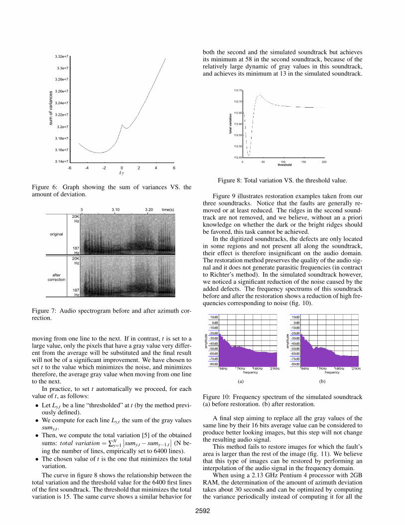
In practice, to set t automatically we proceed, for eachvalue of t, as follows:• Let Ly,t be a line “thresholded” at t (by the method previ-

ously defined).• We compute for each line Ly,t the sum of the gray values

sumy,t .• Then, we compute the total variation [5] of the obtained

sums: total variation = ∑Ny=1

∣∣sumy,t − sumy−1,t∣∣ (N be-

ing the number of lines, empirically set to 6400 lines).• The chosen value of t is the one that minimizes the total

variation.The curve in figure 8 shows the relationship between the

total variation and the threshold value for the 6400 first linesof the first soundtrack. The threshold that minimizes the totalvariation is 15. The same curve shows a similar behavior for

both the second and the simulated soundtrack but achievesits minimum at 58 in the second soundtrack, because of therelatively large dynamic of gray values in this soundtrack,and achieves its minimum at 13 in the simulated soundtrack.

0 50 100 150 200112.45

112.50

112.55

112.60

112.65

112.70

112.75

threshold

tota

l var

iatio

n

Figure 8: Total variation VS. the threshold value.

Figure 9 illustrates restoration examples taken from ourthree soundtracks. Notice that the faults are generally re-moved or at least reduced. The ridges in the second sound-track are not removed, and we believe, without an a prioriknowledge on whether the dark or the bright ridges shouldbe favored, this task cannot be achieved.

In the digitized soundtracks, the defects are only locatedin some regions and not present all along the soundtrack,their effect is therefore insignificant on the audio domain.The restoration method preserves the quality of the audio sig-nal and it does not generate parasitic frequencies (in contractto Richter’s method). In the simulated soundtrack however,we noticed a significant reduction of the noise caused by theadded defects. The frequency spectrums of this soundtrackbefore and after the restoration shows a reduction of high fre-quencies corresponding to noise (fig. 10).

94Hz 7KHz 14KHz 21KHz

frequency

10dB

0dB-10dB

-20dB-30dB-40dB-50dB-60dB-70dB-80dB

ampl

itude

(a)

94Hz 7KHz 14KHz 21KHzfrequency

10dB

0dB-10dB

-20dB-30dB-40dB-50dB-60dB-70dB-80dB

ampl

itude

(b)

Figure 10: Frequency spectrum of the simulated soundtrack(a) before restoration. (b) after restoration.

A final step aiming to replace all the gray values of thesame line by their 16 bits average value can be considered toproduce better looking images, but this step will not changethe resulting audio signal.

This method fails to restore images for which the fault’sarea is larger than the rest of the image (fig. 11). We believethat this type of images can be restored by performing aninterpolation of the audio signal in the frequency domain.

When using a 2.13 GHz Pentium 4 processor with 2GBRAM, the determination of the amount of azimuth deviationtakes about 30 seconds and can be optimized by computingthe variance periodically instead of computing it for all the

2592

(a) (b) (c) (d) (e) (f)

Figure 9: Cut-off of the first soundtrack (a) before restoration. (b) after restoration. Cut-off of the second soundtrack (c) beforerestoration. (d) after restoration. Cut-off of the simulated soundtrack (e) before restoration. (f) after restoration.

Figure 11: A defect present over a large area.

lines. Azimuth correction takes 60 seconds for processing64000 lines. Determining the threshold value takes about 300seconds (if we perform the operations for all the 256 possi-ble thresholds). And the final correction using the obtainedthreshold takes 30 seconds for processing 64000 lines.

5. CONCLUSION

We proposed a new method for the restoration of variabledensity soundtracks. This method provides an accurate az-imuth correction algorithm and a thresholding techniquebased on the minimization of total variation when movingfrom one line of the soundtrack to the next, thus allowing anautomatic parametrization of the method. We are currentlyworking on the development of restoration techniques thattake into account the spatial distribution of defects instead ofprocessing them on each line separately. The effect of badexposure on variable density soundtracks is also of interest.Looking at the frequency domain to perform a restoration ofdefects located over a large area needs to be studied as well.Finally, all these developments have to be integrated into acomplete restoration system that handles all the processes

from the digitization of the soundtrack to the generation ofthe restored audio file.

6. ACKNOWLEDGMENTS

This work has been undertaken within the ResonancesProject (http://www.riam-resonances.org/) and was madepossible thanks to the financial help of the French AgenceNationale de la Recherche, through its RIAM program. Thefilm material, as well as the expertise on motion picture op-tical soundtracks, were provided by N. Ricordel from the“Centre National de Cinematographie-Archives Francaisesdu Film” and by C. Comte from “GTC-Eclair Group”.

REFERENCES

[1] ATMEL Application Note, Flat Field Correction, HowFlat Field Correction and Contrast Expansion are im-plemented in AViiVA cameras. 2005.

[2] ISO2969: B-chain electro-acoustic response of motion-picture control rooms and indoor theatres – specifica-tions and measurements (1987) International standard.

[3] E. Brun, A. Hassaıne, B. Besserer and E. Decenciere,“Restoration of variable area soundtrack,” in Proc. of2007 International Conference on Image Processing,San Antonio, USA. september 2007.

[4] J. G. Frayne, H. Wolfe, Elements of sound recording.John Wiley & Sons, New York, 1949.

[5] S. Osher and L. Rudin, “ Feature-oriented image en-hancement using shock filters,” IEEE transactions on im-age processing vol. 27, pp. 919–940, 1990.

[6] D. Richter, I. Kurreck and D. Poetsch, “Restoration ofoptical variable density sound track on motion picturefilms by digital image processing,” in Proc. of the 7thInternational Conference on Optimization of Electricaland Electronic Equipments, University of Brasov, Ro-mania, 2002.

[7] P. Streule, Digital image based restoration of opticalmovie soundtracks. Master Thesis. ETH Zurich. 1999.

[8] H. M. Tremaine, Audio Cyclopedia. Howard W. Sams &co., Indianapolis, First Printing, 1959.

[9] J. Valenzuela, Digital reproduction of variable den-sity film soundtracks. United states patent 20060232745,2006.

2593