RESTING HABITAT SELECTION BY FISHERS IN CALIFORNIA - fs.fed.us · resting habitat selection by...

RESTING HABITAT SELECTION BY FISHERS IN CALIFORNIA

WILLIAM J. ZIELINSKI,1 USDA Forest Service, Pacific Southwest Research Station, Redwood Sciences Laboratory, 1700Bayview Drive, Arcata, CA 95521, USA

RICHARD L. TRUEX,2 USDA Forest Service, Pacific Southwest Research Station, Redwood Sciences Laboratory, 1700 BayviewDrive, Arcata, CA 95521, USA

GREGORY A. SCHMIDT,3 USDA Forest Service, Six Rivers National Forest, 1330 Bayshore Way, Eureka, CA 95501-3438 USAFREDRICK V. SCHLEXER, USDA Forest Service, Pacific Southwest Research Station, Redwood Sciences Laboratory, 1700

Bayview Drive, Arcata, CA 95521, USAKRISTIN N. SCHMIDT,4 USDA Forest Service, Six Rivers National Forest, 1330 Bayshore Way, Eureka, CA 95501-3438, USAREGINALD H. BARRETT, Department of Environmental Science, Policy and Management, University of California, Berkeley, CA

95720-3110, USA

Abstract: We studied the resting habitat ecology of fishers (Martes pennanti) in 2 disjunct populations in California,USA: the northwestern coastal mountains (hereafter, Coastal) and the southern Sierra Nevada (hereafter, Sierra).We described resting structures and compared features surrounding resting structures (the resting site) with thoseat randomly selected sites that also were centered on a large structure. We developed Resource Selection Functions(RSFs) using logistic regression to model selection of resting sites within home ranges, and we evaluated alterna-tive models using an information–theoretic approach. Forty-five fishers were radiomarked, resulting in 599 restinglocations. Standing trees (live and dead) were the most common resting structures, with California black oak (Quer-cus kelloggii) and Douglas-fir (Psuedotsuga menziesii) the most frequent species in the Sierra and Coastal study areas,respectively. Resting structures were among the largest diameter trees available, averaging 117.3 ± 45.2 (mean ± SE)cm for live conifers, 119.8 ± 45.3 for conifer snags, and 69.0 ± 24.7 for hardwoods. Females used cavity structuresmore often than males, while males used platform structures significantly more than females. The diversity of typesand sizes of rest structures used by males suggested that males were less selective than females. In the Sierra studyarea, where surface water was less common, we found almost twice as many resting sites as random points within100 m of water. Multivariate regression analysis resulted in the selection of RSFs for 4 subsets of the data: all indi-viduals, Sierra only, Coastal only, and females only. The top model for the combined analysis indicated that fishersin California select sites for resting with a combination of dense canopies, large maximum tree sizes, and steepslopes. In the Sierra study area, the presence of nearby water and the contribution of hardwoods were more impor-tant model parameters than in the Coastal area, where the presence of large conifer snags was an important pre-dictor. Based on our results, managers can maintain resting habitat for fishers by favoring the retention of largetrees and the recruitment of trees that achieve the largest sizes. Maintaining dense canopy in the vicinity of largetrees, especially if structural diversity is increased, will improve the attractiveness of these large trees to fishers.

JOURNAL OF WILDLIFE MANAGEMENT 68(3):475–492

Key words: California, fisher, habitat selection, Martes pennanti, resting sites.

475

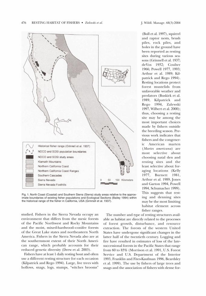
The fisher has been extirpated from extensiveregions of its historical range in the Pacific states(Gibilisco 1994, Powell and Zielinski 1994, Aubryand Lewis 2003). In California, the fisher appearsto occupy less than half of the range it did in theearly 1900s, and the species’ range is divided into2 remnants separated by approximately 400 km(Fig. 1; Zielinski et al. 1995). This separation isalmost 4 times the species’ maximum recordeddispersal distance (York 1996). Fishers occur in

mature, structurally complex, conifer–hardwoodforests and are described as being among themost habitat-specialized mammals in NorthAmerica (Harris et al. 1982, Buskirk and Powell1994). Few studies, however, have attempted toquantify the habitats selected by fishers in thewestern United States.

California is unique among western states inthat fishers have persisted since before Europeansettlement, and the state has received no reintro-ductions from elsewhere. The fisher populationin northwestern California has been the subjectof several previous studies (Buck et al. 1994,Seglund 1995, Klug 1996, Dark 1997), and, al-though the fisher population probably is thelargest in the western United States, it is isolatedfrom other populations (Powell and Zielinski1994, Aubry and Lewis 2003). The ecology of fish-ers in the Sierra Nevada has never been formally

1 E-mail: [email protected] Present address: USDA Forest Service, Pacific South-

west Region, 900 West Grand Avenue, Porterville, CA93257, USA.

3 Present address: Institute for Wildlife Studies, P.O.Box 1104, Arcata, CA 95518, USA.

4 Present address: Redwood National and State Parks,P.O. Box 7, Orick, CA 95555, USA.

J. Wildl. Manage. 68(3):2004476 RESTING HABITAT OF FISHERS • Zielinski et al.

studied. Fishers in the Sierra Nevada occupy anenvironment that differs from the mesic forestsof the Pacific Northwest and Rocky Mountainsand the moist, mixed-hardwood–conifer forestsof the Great Lake states and northeastern NorthAmerica. Fishers in the Sierra Nevada also are atthe southernmost extent of their North Ameri-can range, which probably accounts for theirreduced genetic diversity (Drew et al. 2003).

Fishers have at least 1 daily resting bout and oftenuse a different resting structure for each occasion(Kilpatrick and Rego 1994). Large, live trees withhollows, snags, logs, stumps, “witches brooms”

(Bull et al. 1997), squirreland raptor nests, brushpiles, rock piles, andholes in the ground havebeen reported as restingsites during various sea-sons (Grinnell et al. 1937;deVos 1952; Coulter1966; Powell 1977, 1993;Arthur et al. 1989; Kil-patrick and Rego 1994).Resting locations protectforest mustelids fromunfavorable weather andpredators (Buskirk et al.1989, Kilpatrick andRego 1994, Zalewski1997, Wilbert et al. 2000);thus, choosing a restingsite may be among themost important choicesmade by fishers outsidethe breeding season. Pre-vious work indicates thatfishers and the congener-ic American marten(Martes americana) aremost selective aboutchoosing natal den andresting sites and theleast selective about for-aging locations (Kelly1977, Burnett 1981,Arthur et al. 1989, Jonesand Garton 1994, Powell1994, Schumacher 1999).This suggests that rest-ing and denning sitesmay be the most limitinghabitat element acrossfisher ranges.

The number and type of resting structures avail-able as habitat are directly related to the processesof forest growth, disturbance, and resourceextraction. The forests of the western UnitedStates have undergone significant changes in thelatter half of the twentieth century. Logging andfire have resulted in estimates of loss of the late-successional forests in the Pacific States that rangefrom 60 to 85% (Morrison et al. 1991, U.S. ForestService and U.S. Department of the Interior1993, Franklin and Fites-Kaufman 1996, Beardsleyet al. 1999). The use by fishers of large trees andsnags and the association of fishers with dense for-

Fig. 1. North Coast (Coastal) and Southern Sierra (Sierra) study areas relative to the approx-imate boundaries of existing fisher populations and Ecological Sections (Bailey 1994) withinthe historical range of the fisher in California, USA (Grinnell et al. 1937).

J. Wildl. Manage. 68(3):2004 477RESTING HABITAT OF FISHERS • Zielinski et al.

est cover (Carroll et al. 1999, Weir and Harestad2003) would appear to make fishers especiallyvulnerable to these changes in forest ecosystems.

Our goal was to characterize the resting habitatfeatures selected by fishers in California and tocontrast the resting habitat features selected byfishers in the northern Coast Range and those inthe southern Sierra Nevada. This information willenable managers and researchers to tailor theirrecommendations about the habitat needs of fish-ers to specific regions of interest and to developmethods to assess habitat conditions in each area.New information about fisher resting-site selectionin California will also shed light on the perceiveddifferences in the use of mature and old-foreststands in western and eastern North America.Research in the western United States indicatesthat fishers are associated with extensive matureconifer forests and that large woody elements ofthese forests are requirements (e.g., Harris et al.1982, Buck et al. 1994, Jones 1991, Weir andHarestad 2003). In contrast, research in the north-eastern and midwestern United States suggests thatmid-successional, mixed broad-leaved and conifer-ous forests provide suitable fisher habitat (Arthuret al. 1989, Buskirk and Powell 1994, Krohn 1994).

STUDY AREAS Our 2 study areas (Fig. 1) are in the Humid Tem-

perate Domain, Mediterranean Division, and theSierran Steppe–Mixed Forest Coniferous ForestProvince (Bailey 1994). The Sierra study area lieswithin the Sierra Nevada and the Sierra NevadaFoothills Sections, while the Coastal study area iswithin the Northern California Coast Ranges Sec-tion (Bailey 1994). Weather patterns in both areasare typical of California’s Mediterranean climate:summers are hot and dry, while winters are cooland moist, with precipitation often falling as snowin the higher elevations. Despite these similarities,differences in proximity to the Pacific Ocean andlatitude (Fig. 1) have resulted in important differ-ences between the areas. The Coastal study areawas located within 50 km of the Pacific Ocean andreceived more precipitation, resulting in denseand continuous forest cover; the southerly locationand lower precipitation in the Sierra area haveresulted in a landscape with greater heterogeneity.

The Coastal study area was in Humboldt andTrinity counties on approximately 400 km2 of theSix Rivers and Shasta-Trinity national forests. Wecollected data May 1993–September 1997. Thestudy area included 2 subareas: the northernPilot Creek and the southern Cedar Gap (Fig. 1).

Topography in the Pilot Creek area was dominat-ed by South Fork Mountain, a 72-km-long con-tinuous ridge joining the 2 subareas. Elevationsranged from approximately 600 to 1,800 m, andthe area was vegetated by stands of Douglas-fir,white fir (Abies concolor), Oregon white oak (Quer-cus garryana), tanoak (Lithocarpus densiflora), redfir (A. magnifica), and dry grasslands, with a minorcomponent of California black oak, canyon liveoak (Q. chrysolepis), incense cedar (Calocedrusdecurrens), and ponderosa pine (Pinus ponderosa;U.S. Forest Service 1995, Jimerson et al. 1996).

The Sierra study was conducted on 300 km2 inthe Sequoia National Forest in Tulare County(Fig. 1). Data were collected during April1994–October 1996. Elevations ranged fromapproximately 800 m in the west-slope foothills toover 3,000 m at the southern Sierra Nevada’sGreat Western Divide. The primary vegetationtypes (Mayer and Laudenslayer 1988) were Sier-ran mixed conifer, ponderosa pine, red fir, mon-tane hardwood, and various chaparral types.Lodgepole pine (Pinus contorta), Jeffrey pine (P.jeffreyi), and grassland/meadow types composeda small minority of the area. Stands characterizedby trees averaging >30-cm diameter at breastheight (dbh) occurred over 56% of the area;stands with trees averaging >61-cm dbh occurredover 10% of the area. Clearcutting has been thetraditional silvicultural method in the Coastalstudy area (U.S. Forest Service and U.S. Depart-ment of the Interior 1993), whereas individual-treeselection harvest is more common in the southernSierra Nevada (McKelvey and Johnson 1992).

METHODS

Animal Capture and HandlingWe initially trapped fishers in areas where they

had been detected at track plate survey stations(Zielinski and Kucera 1995) and throughout ourstudy area where habitat appeared suitable. Weused Tomahawk live traps (model 207, Toma-hawk Live Trap Company, Tomahawk, Wisconsin,USA) modified with a plywood cubby boxattached to the closed end to provide shelter. Webaited traps with chicken and a commercial scentlure (M & M Fur Company, Bridgewater, SouthDakota, USA), and we checked traps daily. Toprevent detaining females near the time of par-turition and early stages of kit rearing, we did nottrap between late March and early May. We con-ducted additional trapping to replace failedradiotransmitters or to capture new animals.


We restrained fishers in a metal handling coneand sedated them with a ketamine hydrochlorideand Diazepam mixture (10 mL ketamine/5 mLDiazepam); animals typically received 0.15–0.20mL/kg body mass. Once immobilized, animalswere sexed, measured, weighed, ear-tagged, andphotographed. Fishers were fitted with Telonics(Mesa, Arizona, USA) model 80 radiotransmit-ters for females and model 125 radiotransmittersfor males.

Animal RelocationRadiomarked Animals, Walk-in Surveys.—Using

hand-held receivers and antennas, we attemptedto relocate all radiomarked fishers at least onceper week using walk-in surveys (direct approachesto attempt to visually locate resting animals). Weconducted walk-in surveys by following the signalof animals whose radiotransmission indicated thatthey were inactive for at least 30 min prior to thestart our survey. We categorized 14 resting-struc-ture types: cavity in live tree, broken top in livetree, unknown location in live tree, cavity in snag,broken top in snag, unknown location in snag,stump, animal nest, mistletoe and witches brooms(Bull et al. 1997), logs, coarse woody debris pile,subnivean site, ground burrow, and rock pile.When the radio signal confirmed the location of afisher to a particular live tree or snag with con-spicuous cavities, and the animal was unlikely to behidden in dense canopy, we assumed that the fish-er was occupying a cavity in the tree. When oursearch resulted in the visual confirmation of a rest-ing fisher, we were able to relate the characteristicsof the signal to the distance from the animal.This experience indicated that our error was usu-ally <10-m horizontal distance. Often the errorwas less because numerous sites could be excludedfrom consideration since all possible resting loca-tions were visible. Snow restricted access to theCoastal study area from the ground during thewinter, so a smaller proportion of locations werecollected during this time from the Coastal thanfrom the Sierra area. Natal and maternal denswere identified when the pattern of resting-struc-ture use by a female changed from multiple sitesto 1 site during the early spring or when kits wereobserved with an adult. We did not include struc-tures known to be used as natal and maternal densin the resting-structure or resting-site analysis.

Habitat SamplingWe developed habitat sampling protocols to

collect data on (1) characteristics reported in the

literature to be important to fishers, (2) featuresthat differed between the 2 study areas, and (3)habitat conditions that may be unique to fishersin California. We grouped variables into 6 families:topographic, vegetation cover type, tree abun-dance, tree size, ground cover, and canopy closure.

Sampling Used Resources.—When we located rest-ing animals in live trees and snags, we recordedtree species, dbh (1.4 m), estimated height (m),estimated height of resting structure (m), andcondition class (Maser et al. 1979). For logs, werecorded the species, estimated maximum diame-ter (cm), minimum diameter (cm), and totallength (m), measured log aspect, and assignedthe log a decay class (Maser et al. 1979). Thespecies of standing trees used as resting struc-tures were aggregated based on growth charac-teristics and functional form. Due to the absenceof Douglas-fir in the Sierra area, this species wasconsidered a unique category for the Coastalarea. Common to both study areas were the fol-lowing groups: hardwoods (California black oak,interior [Quercus wislizenii] and canyon live oak,madrone [Arbutus menziesii], chinquapin [Chrysolep-sis chrysophylla], and tanoak), pines (sugar [Pinuslambertiana], ponderosa, and Jeffrey), true firs(red and white fir), and other conifers (incensecedar, unknown conifers, and, for the Sierra area,giant sequoia [Sequoiadendron giganteum]).

We described habitat at the resting site as thevegetation and landscape characteristics in theimmediate vicinity of the resting structure. Theresting structure was plot center for these mea-surements. We recorded aspect using a compassand percent slope by averaging the uphill anddownhill clinometer recordings. Topographicalposition of the resting structure was categorizedas ridge top, mid-slope, or drainage bottom, andwe estimated the distance to water if it was within100 m of the resting structure. One-hundredmeters was the distance over which the water-course appeared to most directly influence theforest structure and composition. For sites locat-ed during the snow season, we recorded the snowdepth surrounding the resting site by averaging 4measurements 10 m from the structure in eachcardinal direction. At both study sites, we appliedthe California Wildlife Habitat Relationships(CWHR) system to assign a habitat type, size class,and canopy cover to the area surrounding theresting structure (Mayer and Laudenslayer 1988).

We conducted variable radius sampling using a20-factor prism to describe aspects of forest struc-ture and composition included in the tree-abun-


dance and tree-size variable families. For all livetrees and snags in the prism sample, we recordedthe species and dbh (minimum = 16 cm), and weestimated height and condition class using thesame categories as for resting structures. We usedline intercept sampling to describe ground-levelattributes. Two 25-m line intercept transects wereplaced perpendicular to each other; transectplacement was based on a random azimuth. Forevery 1-m increment, we measured cover by smalltrees (<7-cm dbh), shrubs, and coarse woodydebris. For each meter interval with shrub cover,we recorded shrub species and visually estimatedheight. Coarse woody debris included all deadand down woody material with estimated mini-mum diameter ≥15 cm. For all dead and downmaterial >30-cm minimum diameter, we estimat-ed total length, maximum and minimum diame-ter, and decay class (Maser et al. 1979). Percentground cover by litter, rock, snow, and herba-ceous vegetation was recorded at every other 1-minterval using a 30 × 30-cm cover square. At theend of each transect and at plot center (the rest-ing structure), we used a spherical densiometerto estimate total percent cover of overhead vege-tation. Most habitat features were sampled within2 weeks of locating a resting structure.

Sampling Available Resources.—We developed aset of criteria to select individuals for which wehad collected sufficient information to include inresource-selection analysis. We selected “focal”animals for analysis that had been (1) monitoredfor at least 10 months; (2) relocated at a mini-mum of 10 resting locations; and (3) relocated,using any location type, a minimum of 20 times.For these animals, we calculated 100% MinimumConvex Polygon (MCP) home-range estimatesusing program CALHOME (Kie et al. 1996). Weused a Geographic Information System (GIS) togenerate 20 random Universal Transverse Mer-cador coordinates within each focal animal’shome range. To sample available habitat, we ori-ented as closely as possible to GIS-generated ran-dom coordinates, and we then selected a randomazimuth and distance (10–50 m) to locate a start-ing point. We used a modified T-square samplingapproach (Besag and Gleaves 1973) to locate astructure-centered random point. First, wesearched >12.5 m from the starting point for thenearest tree or log with size characteristics similarto those of trees and logs used by fishers at eachstudy area. A circle was drawn with a radius equalto the distance from the starting point to the firststructure. The structure selected as the center of

the random plot was the closest structure thatmet the minimum size requirements that was alsooutside a line tangent to the circle.

For the Sierra study area, conifers were candi-date structure points if >76-cm dbh, hardwoods if>42-cm dbh, and logs if >80-cm maximum diam-eter. For the Coastal study area, minimum sizeswere conifers >80-cm dbh, hardwoods >56-cmdbh, and logs >62-cm diameter. The final struc-ture category was conifers with conspicuous plat-forms (e.g., accumulation of litter on branches),which were eligible if they exceeded 30-cm dbh.Platforms had to be capable of supporting a rest-ing fisher and of the minimum diameter criteri-on. Each minimum was 1 standard deviation lessthan the mean for resting sites of the corre-sponding type.

We collected vegetation data at random sitesduring May–October 1996 on the Sierra studyarea and during May–September 1997 on theCoastal study area. We collected habitat data atrandom sites using a similar protocol as was usedat resting sites. Identical methods were used for 5of 6 variable families. Line-intercept transectswere used only to tally the number of logs at ran-dom sites, rather than to record the total amountof intercept, and transect distance was pacedinstead of measured. Shrub cover was estimatedby visual observation.

Because giant sequoias are so much larger thanany other tree species, and they only occur on theSierra area, they would affect some variables wewished to compare between study areas. Eighty-three resting and random sites included ≥1 giantsequoia. Including giant sequoias in the estima-tion of 6 tree-diameter variables (total, conifer,maximum, standard deviation, quadratic mean,quadratic mean of conifer) significantly in-creased each variable (t > 9.0 and P < 0.001 for allcomparisons). We excluded giant sequoias fromthe calculations of dbh but retained them to cal-culate basal area because of their influence onstand density and cover.

Rest-structure AnalysisWe aggregated the 14 structure types into 5

functional groups: live trees (cavities, broken tops,unknown locations in live trees); snags (cavities,broken tops, stumps, unknown locations in deadtrees); platforms (nests, mistletoe growths, witch’sbrooms); logs (individual logs and coarse woodydebris piles); and ground cavities (subnivean sites,ground burrows, rock piles). These classes werefurther aggregated to the coarse categories of


standing trees (live and dead) and ground struc-tures (logs and ground cavities). Comparisons ofresting structures between sexes and study areaswere conducted by calculating frequency distrib-utions and using chi-square statistics.

Habitat-selection AnalysisComparisons of used and available resources

are standard in habitat-selection studies, but fewhave examined the potential influence that phys-ical characteristics of the used location may haveon surrounding habitat. When the used structurerepresents an uncommon feature of the habitat(e.g., large tree or snag), the structure itself caninfluence surrounding habitat characteristics(e.g., Sieg and Becker 1990, Jones 2001). Becausefishers often rest in large trees (Powell and Zielin-ski 1994), the presence of these features caninfluence the surrounding vegetation. We exam-ined habitat selection at the rest site by compar-ing used sites to random sites conditioned on thepresence of a large central woody structure (e.g.,Edwards and Collopy 1988).

We collected a sample of used sites (restinglocations) and available sites (randomly selectedlocations) from individual animals, and we usedRSF analysis (Manly et al. 1993) to identify char-acteristics that distinguished sites where fishersrested from available sites. The analyses were ret-rospective in that a sample of use data was col-lected and a second, independent sample ofavailable resources was collected later. The esti-mated RSFs took the form:

W(x) = exp(β1x1 + β2x2 + ...βnxn),

where W(x) is the relative probability of resourceuse for the given combination of covariates (Xi),and slopes (Bi) are estimated using maximum-likelihood methods. The data were analyzedusing logistic regression (SAS Institute 1990).The intercept in the RSF was treated as a nui-sance parameter and excluded from the logisticmodel (McCullagh and Nelder 1989).

Habitat Characteristics at Used and AvailableSites.—After developing a set of over 100 variablesto describe habitat surrounding used and avail-able sites, we reduced the pool of potential vari-ables using the following criteria: field repeatabil-ity, the magnitude of variances, multicollinearity,univariate comparisons of mean values, and thosethat the literature suggested had biological andmanagement relevance. Throughout the process,we placed greater emphasis on retaining physiog-

nomic rather than floristic variables, consistentwith the conclusions of previous habitat studies onfishers and martens (Buskirk and Powell 1994).

For a subset of continuous variables, we calcu-lated descriptive statistics for resting and randomsites. We used t-tests, controlling the Type I errorrate for the number of comparisons (α =0.05/no. of comparisons), to conduct univariatetests of differences between the mean value of avariable at resting sites and at random sites. Forcontinuous variables, the means were generatedfrom the mean values for a site type for individualfocal animals. Differences between site types forcategorical variables were analyzed by pooling allsite types for all individuals and evaluated usingeither contingency tables or Fisher’s exact test(Zar 1984). We used the results of these analysesto describe habitat and to guide variable selec-tion for RSF analysis (Manly et al. 1993).

Variable Reduction, Data Pooling, and Resource Selec-tion Functions.—We conducted univariate logisticregression for each variable to assess the potentialimportance of individual variables in distinguish-ing used from available sites. Variables with signif-icant slopes (P < 0.25 threshold; Hosmer andLemeshow 1989) were retained. We developed 4multivariate RSFs that represented 3 levels ofdata aggregation: (1) all individuals—referred toas the Fisher model; (2) all individuals withineach study area—referred to as the Coastal andSierra models; (3) all females—referred to as theFemale models. We were unable to monitor suffi-cient males to develop a RSF for this sex.

Development of the RSF models involved sever-al steps. First, to identify candidate models foreach of the 4 analyses, we conducted best subsetslogistic regressions (Hosmer and Lemeshow1989), selecting the best 3 logistic models with3–8 predictor variables (i.e., the best 3 modelsusing 3 predictor variables, the best 3 modelsusing 4 predictor variables, etc.). For this analysis,data were pooled across individuals prior tomodel fitting. This resulted in a total of 21 candi-date models for each of the 4 selection analyses.We evaluated models that were constructed onlyfrom the smallest subset of variables that we con-sidered biologically important for fishers, ratherthan exploring all possible subsets of variablecombinations (Anderson and Burnham 2002).

Second, for each of the 21 candidate modelsper selection analysis, we fitted each model toeach individual focal fisher and calculatedAkaike’s Information Criterion adjusted for smallsample size (AICc; Akaike 1973, Burnham and


Anderson 2002). For each candidate model, wesummed AICc values across fishers and calculatedAkaike weights. We identified top models basedon Akaike weights, and if the model with the low-est AICc value also accounted for >90% of theAkaike weights, it was selected as the best model.Otherwise, we identified top models whosecumulative Akaike weights were >0.90 (Burnhamand Anderson 2002).

Finally, we estimated parameters for each RSFmodel. For selection analyses where a single topmodel was identified (i.e., Akaike weight > 0.90),we calculated a weighted average of parameterestimates from the top model for each fisher,where the weight was the inverse of the standarderror of the parameter (i.e., precise estimateswere weighted more heavily than less precise esti-mates). For selection analyses that did not identifya single top model, we calculated the model-weighted parameter estimates for each fisherusing renormalized Akaike weights to estimateparameters and their unconditional standarderrors (Burnham and Anderson 2002). Final RSFparameter estimates were calculated as above butwere weighted by the inverse of the uncondition-al sampling variance.

We eliminated models for some RSF analyseswhen variables were included for which completeor quasi-complete separation of data points exist-ed. This form of overdispersion occurred when asite type lacked representation from 1 or theother state of a nominal scale variable (e.g., pres-ence/absence of large snags, presence/absence

of water <100 m fromsite). Under these con-ditions, maximum likeli-hood parameter esti-mates for some or allvariables did not exist.

Assessing Model Perfor-mance.—We examinedthe performance of finalmodels using data fromanimals that were notincluded in developingthe models (i.e., non-focal animals and datafrom focal animals thatwere excluded due tothe problem of com-plete separation of datapoints). Relative predict-ed probabilities werecalculated using the

appropriate final RSF, and data for all observa-tions were rescaled such that the maximum rela-tive predicted probability of use assumed a valueof 1. We did not attempt to classify test sites as usedor unused and instead examined the distributionof relative probabilities for used and random sites.

RESULTS

Animal Capture and RelocationWe radiomarked 45 fishers, 23 (8 M, 15 F) on

the Sierra and 22 (8 M, 14 F) on the Coastal studyarea. We located resting fishers 397 times at 338structures on the Sierra study area and 202 timesat 195 structures on the Coastal study area. Of theradiomarked animals, 12 (4 M, 8 F) on the Sierrastudy area and 9 (2 M, 7 F) on the Coastal study areamet our criteria as focal animals. Resting-site relo-cation was less successful during the snow seasonthan the snow-free season (Table 1). The number ofresting sites located for focal individuals rangedfrom 10 to 69 with a mean of 23.5 per animal.

Resting-structure UseThirty-six fishers (13 M, 23 F) used resting struc-

tures on 599 occasions. This includes 66 occasionswhen an individual reused a structure it had usedpreviously (excluding reuses of natal or maternaldens). We observed fishers (visual or audible) at191 of the 599 occasions. Unknown locations inlive trees comprised 63.4 and 34.6% of the live-treecategory in Coastal and Sierra, respectively. Livetrees constituted 46.4% of the resting structures

Table 1. Mean (SD) values for the number of resting sites and habitat plots sampled per indi-vidual fisher for each season. Data are summarized separately for each study area (Coastal:Six Rivers National Forest, California, USA, May 1993–Sep 1997; Sierra: Sequoia NationalForest, California, USA, Apr 1994–Oct 1996) and for males and females. The total number ofsites is summarized at the bottom of table where data from focal animals are distinguishedfrom non-focal animals. Resting sites reused by different individuals, or by the same individ-ual at least 7 days apart, contribute to totals. Summer is the period from 16 Apr to 31 Oct, andwinter is the period from 1 Nov to 15 Apr.

Study Resting sites Habitat plots area Sex Summer Winter Summer Winter

Coastal Both 14.4 (8.7) 2.7 (1.8) 13.1 (5.5) 2.6 (1.7)Females 11.7 (4.7) 2.6 (2.0) 11.7 (4.7) 2.6 (2.0)Males 24.0 (15.6) 3.0 (1.4) 18.0 (7.1) 2.5 (0.7)

Sierra Both 20.6 (14.0) 7.7 (7.5) 15.8 (10.7) 6.2 (5.7)Females 24.8 (15.6) 9.4 (8.7) 19.3 (11.6) 7.4 (6.5)Males 12.3 (2.5) 4.3 (2.6) 9.0 (2.9) 3.8 (3.1)

Both Both 18.0 (12.1) 5.5 (6.2) 14.7 (8.8) 4.6 (4.7)Females 18.7 (13.3) 6.2 (7.2) 15.7 (9.6) 4.8 (5.4)Males 16.2 (9.4) 3.8 (2.2) 12.0 (6.1) 3.3 (2.5)

Total resting sites and habitat plots Focal 377 116 308 97Non-focal 93 13 60 9Combined 470 129 368 106


used by fishers. Douglas-fir accounted for 65.6% ofall resting sites located in the Coastal study area.Hardwoods comprised nearly 45% of all restinglocations, and California black oak was the pre-dominant species (approx 85% of hardwoodsspecies used). Black oaks produce cavities thatwere used regularly for resting by fishers in bothareas, but they were used more frequently in theSierra (37.5% of all resting structures) than theCoastal area (10.9% of resting structures). Theaverage size of resting structures, within type, wassimilar for all sex × study area combinations(Appendix A). Live conifers and snags were thelargest structures used (x– = 117.3-cm dbh, for liveconifers; x– = 119.8-cm dbh for conifer snags;Appendix A). Resting-structure reuse was lowoverall, but higher in the Sierra (55 reuses, 13.8%)than in the Coastal (7 reuses, 3.5%) study area.

The sexes did not use all structure types simi-larly (χ2 = 31.86, P < 0.001), presumably due tothe greater use of platforms by males (16.8 vs.8.3%) and the more frequent use of snags byfemales (31.7 vs. 18.0%). Study area also signifi-cantly affected the distribution of resting-struc-ture use (χ2 = 22.93, P < 0.001), due primarily tothe differential use of platforms (Coastal: 18.3%,Sierra: 6.8%). Males used platforms significantlymore than females, and females in the Coastalstudy area used platforms significantly more(14.3%) than females in the Sierra study area(5.9%; χ2 = 9.64, P = 0.046).

Resting-site Habitat Characteristics Univariate Vegetation Analyses.—Initial variable

reduction resulted in the retention of 5 topo-graphic, 3 vegetation type, 11 tree abundance, 2canopy closure, 10 tree size, and 4 ground-covervariables (Table 2). Using the data from focal andnon-focal individuals, resting sites had signifi-cantly larger maximum dbh, average canopy clo-sure, and shrub canopy closure, more largesnags, and steeper slope than random sites. Rest-ing sites also had significantly more variable treedbhs and significantly less variable canopy closures(Table 3). Conifers and hardwoods were smallestat random sites, larger at resting sites, and largestwhen used as resting structures (Fig. 2). The 2study areas differed in respect to the variablesthat were significantly different at rest and ran-dom sites, and in respect to the characteristics ofthe sites used for resting (Table 3). Most restingand random sites at both study areas were in theDense CWHR canopy category (>60% canopy clo-sure). Tree size class 5 (>61.0-cm dbh) was the

most frequent tree size class at resting sites in theCoastal area, whereas class 4 (28.0–61.0 cm) wasthe most frequent class in the Sierra. We found noconspicuous differences in CWHR tree size classamong site types in either study area. All measuresof basal area and the frequency of large snags weregreater at resting sites used by females compared tomales, though the tree dbh was similar (Table 3).

Resource Selection FunctionsOnly data from focal animals were used to esti-

mate RSFs. This included 21 animals (6 M, 15 F; 9and 12 from the Coastal and Sierra areas, respec-tively), although 1 female from the Sierra area wasdropped from consideration due to complete sep-aration of data points. Twelve variables were can-didates for inclusion in the 4 selected RSFs(BA_LARGE, BA_SMALL, BACON, BAHDW,BARS, CANAVE, CANSTD, DBHMAX, DBHSTD,DBHAVE, DBHAVEH, SLOPE, WATER, CON-SNAG; see Table 2 for definitions).

Fisher Models.—A single model accounted for>0.90 of the Akaike weight (Table 4) and took theform:

W(x) = exp(0.0618*CANAVE + 0.0153*DBH-MAX + 0.0229*SLOPE).

This function indicates that fishers in Californiaselect sites with denser canopies, a larger maxi-mum tree size, and steeper slopes (Tables 4, 5).Predictive power was moderate (R2 = 0.31), andoverall resting habitat use patterns varied consid-erably among individuals, but the concentrationof Akaike weight suggests that resting habitat useby our study animals is influenced by a relativelysimple combination of 3 variables that includebiotic and abiotic features.

Coastal Models.—A single model accounted for>0.90 of the Akaike weight (Table 4) and took theform:

W(x) = exp(0.06496*CANAVE + 0.01437*DBH-MAX + 0.8692*CONSNAG).

Resting sites in the Coastal study area were bestdistinguished from random sites on the basis ofgreater canopy closure, larger maximum treesize, and the presence of at least 1 large (>102-cmdbh) conifer snag (Tables 4, 5). Inclusion of theconifer snag variable distinguished the topCoastal model from the top Fisher model. Thenext most competitive Coastal models (∆AICc =5.92 and 7.44, respectively) included the variables


Table 2. Definitions and acronyms for variables recorded at resting structures and random sites within fisher home ranges in theCoastal (Six Rivers National Forest) and Sierra (Sequoia National Forest) study areas during May 1993–Sep 1997 and Apr1994–Oct 1996, respectively.

Variable Acronym Measurement technique / definition

Topographic variables Percent slope SLOPE Clinometer; average of uphill and downhill Elevation ELEV Altimeter (m) Topographic position TOPOG Estimated: ridge, mid or drainage Aspect A Compass Distance to water WATER < or > 100 m

Vegetation cover type variables CWHRa habitat type CWHRTYPE Estimating using CWHR guide CWHR habitat size class CWHRSIZE Estimating using CWHR guide CWHR canopy closure CWHRCC Estimating using CWHR guide

Tree abundance variables Total basal area BA 20-factor prism (m2/ha) Basal area large trees BA_LARGE m2/ha of trees > 52 cm dbhb

Basal area small trees BA_SMALL m2/ha of trees ≤ 51 cm dbh Basal area trees >102-cm dbh BA5 m2/ha of trees >102-cm dbh Basal area conifers BACON m2/ha of conifers Basal area large conifers BACONL m2/ha of conifers >52-cm dbh Basal area small conifers BACONS m2/ha of conifers ≤51-cm dbh Basal area hardwoods BAHDW m2/ha of hardwoods Basal area live trees BALIVE m2/ha of non-snags Basal area resting-site sized trees BARS Sierra: m2/ha of hardwoods >42-cm dbh and conifers >72-cm dbh;

Coastal: m2/ha of hardwoods >56-cm dbh and conifers >79-cm dbh Basal area snags BASNAG m2/ha of standing dead trees

Canopy closure variables Average canopy closure CANAVE Mean of densiometer readings at 5 plot locations Canopy closure standard deviation CANSTD Standard deviation of densiometer readings at 5 plot locations

Tree size variables Average conifer dbh DBHAVEC Mean dbh (cm) of conifers in the prism sample Average hardwood dbh DBHAVEH Mean dbh (cm) of hardwoods in the prism sample Average dbh DBHAVE Mean dbh (cm) of all trees in the prism sampleMaximum dbh DBHMAX Dbh (cm) of the tree with the largest dbh on the plot; including the rest-

ing structureConifer quadratic mean dbh DBHQMC Quadratic mean diameter (cm) of conifersQuadratic mean dbh DBHQM Quadratic mean diameter (cm)Standard deviation dbh DBHSTD Standard deviation of mean dbh (cm)Average tree height TRHTAVE Mean height (m) of trees in the prism sampleTree height standard deviation TRHTSTD Standard deviation of height (m) of trees in the prism samplePresence large conifer snag CONSNAG Presence of ≥1 conifer snag >102-cm dbh

Ground cover variables Number of logs NOLOGS Number of logs >15-cm diameter at smallest end Number of large logs NOLOGS_L Number of logs >60-cm diameter at smallest end Number of small logs NOLOGS_S Number of logs >15-cm diameter and <30-cm diameter at smallest end Estimated shrub cover SHRUBCC Observer estimated percent shrub cover

a CWHR = California Wildlife Habitat Relationships.b dbh = diameter at breast height.

slope and water, reinforcing the influence oftopographic features on resting-site use.

Sierra Models.—No single model accounted for>0.90 of the Akaike weight so we averaged the 2models that together accounted for >0.90 of theweight (Table 4). This resulted in a model thattook the form:

W(x) = exp(0.0149*DBHMAX + 0.0301*DBH-STD + 0.0194*SLOPE + 0.7663*WATER).

Vegetation structure was represented in themodel by the maximum and standard deviationof tree dbh, whereas slope and the presence ofwater within 100 m indicated the role of topogra-phy in explaining resting-site selection in thesouthern Sierra Nevada (Tables 4, 5). Topograph-ic variables would appear to be important becauseslope and water were both represented in each ofthe models that were averaged. Unique to theSierra models, also, was the frequency with which


Table 3. Select habitat characteristics for resting and randomsites for fishers studied in the Coastal (Six Rivers National For-est, California, USA, May 1993–Sep1997) and Sierra (SequoiaNational Forest, California, USA, Apr 1994–Oct 1996) studyareas. Summary statistics calculated based on mean values for15–20 observations/individual fisher (n = 21 fishers). An asteriskafter mean values in the random column indicates that the vari-able is statistically different than the mean resting value. T-tests(α < 0.0033; 0.05/13 variables) were used for the continuousvariables and chi-square tests for the categorical variables.

No. of Resting Random Variable Pooling fishers Mean SD Mean SD

Continuous Basal area All 21 65.8 11.58 59.9 8.60

(m2/ha) Female 15 69.0 9.72 61.3 9.02 Male 6 58.0 13.01 56.4 6.89 Coastal 9 71.9 11.76 57.8 10.09Sierra 12 61.3 9.53 61.5 7.37

Conifer All 21 51.2 11.79 45.6 10.96 basal Female 15 53.9 12.37 45.4 11.53 area Male 6 44.4 7.14 46.2 10.37 (m2/ha) Coastal 9 55.5 14.53 42.1 9.74

Sierra 12 48.0 8.54 48.2 11.48 Hardwood All 21 14.5 6.74 14.1 6.82

basal Female 15 14.8 6.91 15.7 7.20 area Male 6 13.6 6.84 10.0 3.67 (m2/ha) Coastal 9 16.0 5.68 15.2 5.88

Sierra 12 13.3 7.48 13.2 7.59 Average All 21 62.9 12.54 56.3 9.94

dbh (cm) Female 15 62.4 12.71 54.4 10.61 Male 6 64.2 13.19 61.1 6.49 Coastal 9 70.7 8.97 61.2 9.74 Sierra 12 57.2 11.93 52.7 8.78

Maximum All 21 131.2 22.58 111.0* 15.89 dbh (cm) Female 15 132.3 25.45 110.1* 17.65

Male 6 128.3 14.58 113.3 11.35 Coastal 9 147.7 18.20 119.1* 14.76 Sierra 12 118.8 17.20 104.9* 14.35

Average All 21 93.4 5.07 88.8* 5.45 canopy Female 15 94.7 1.63 90.3* 3.77closure Male 6 90.1 8.79 85.0 7.41(%) Coastal 9 95.0 1.62 86.7 7.29

Sierra 12 92.1 6.40 90.3 3.03Slope (%) All 21 49.8 8.25 42.6* 6.87

Female 15 49.0 8.78 42.4 7.64Male 6 51.9 6.94 43.0 5.02Coastal 9 47.4 8.66 42.8 7.16 Sierra 12 51.5 7.82 42.4 6.97

Basal area All 21 33.4 9.54 32.78 10.03 small Female 15 34.6 7.91 35.30 10.04 trees Male 6 30.5 13.25 26.46 7.28(m2/ha) Coastal 9 30.4 5.10 27.58 9.54

Sierra 12 35.6 11.57 36.67 8.84Basal area All 21 19.5 6.69 18.43 4.80

large Female 15 20.3 6.94 17.98 5.27trees Male 6 17.6 6.13 19.56 3.53(m2/ha) Coastal 9 23.6 6.85 19.87 5.72

Sierra 12 16.5 4.84 17.36 3.90Basal area All 21 10.0 3.08 8.66 2.51

snags Female 15 10.9 2.98 8.70 2.86(m2/ha) Male 6 7.9 2.38 8.54 1.50

Coastal 9 9.3 2.60 6.89 2.16Sierra 12 10.5 3.43 9.98 1.89

Standard All 21 36.0 7.03 29.58* 4.64deviation Female 15 36.5 7.75 29.33* 5.32

Table 3. continued.

No. of Resting Random Variable Pooling Fishers Mean SD Mean SD

dbh Male 6 34.6 5.11 30.22 2.50 Coastal 9 40.5 3.75 32.06* 4.60 Sierra 12 32.6 7.07 27.72 3.87

Standard All 21 6.0 3.00 8.07* 1.94 deviation Female 15 5.1 1.28 7.95* 2.05 canopy Male 6 8.3 4.76 8.34 1.76

Coastal 9 4.7 1.16 8.74* 2.47 Sierra 12 7.0 3.58 7.56 1.32

Shrub All 21 15.0 9.30 27.15* 10.05 canopy Female 15 14.0 9.55 26.95* 11.31 closure Male 6 17.5 8.93 27.65 6.71

Coastal 9 15.8 9.85 28.07 8.35 Sierra 12 14.3 9.25 26.47* 11.48

Categorical Resting Random Pooling n % n %

Presence of large (>102cm dbh) conifer snags (percent of sites)

All 452 40.9 382 23.8* Female 332 45.8 285 22.5* Male 120 27.5 97 27.8 Coastal 176 47.2 188 22.8* Sierra 276 36.9 194 24.7*

Presence of water within 100 m (percent of sites)

All 452 48.4 385 35.1* Female 332 50.6 288 32.6* Male 120 42.5 97 42.3 Coastal 176 44.3 191 42.2 Sierra 276 51.9 194 27.8*

the average dbh of hardwoods (DBHAVEH)appeared in the candidate models (22 of 24 mod-els). This variable was not included in the topmodel, however, because it did not appear ineither of the 2 models that were averaged.

Female Models.—A single model accounted for>0.90 of the Akaike weight (Table 4) and took theform:

W(x) = exp(0.0743*CANAVE + 0.0138*DBHMAX+ 0.0263*SLOPE + 0.8923*CONSNAG).

Female fishers selected resting sites that haddenser canopies, larger trees, were on steeperslopes, and included large conifer snags comparedto random sites within their home ranges (Tables4, 5). The next most competitive model (∆AICc =5.56) included the same variables, except that thepresence of a large conifer snag was excluded.

Model Performance.—We evaluated the top RSFsusing data from 84 resting sites and 22 randomsites that were not used to develop the models.The models were reasonably effective at distin-guishing known resting sites from random sites,


despite the small sample of random-site test dataavailable (Fig. 3). In each set of models, the pre-dicted values for the random sites were always dis-tributed at lower values than the resting sites, andfew random points had scaled relative probabili-ties of selection that exceeded 0.80. Importantly,the distribution of predicted values at restingsites was skewed toward values >0.60 for all mod-els except the Sierra (Fig. 3).

DISCUSSION Our results address several levels of habitat selec-

tion made by adult fishers after they have chosen ahome range. Resting-habitat selection involves thechoice of resting structures within stands as well asthe vegetation and topographic characteristics inthe vicinity of the structure, the resting site. Ourstudy provides a unique opportunity to under-stand the influence of geographic location on

resting-habitat selection because a similar num-ber of fishers were studied at each area, usingidentical methods applied over the same period.

Resting-structure UseMost resting structures at both of our study

areas were in standing trees, and most of thesewere large (x– > 100-cm dbh). Trees used as rest-ing structures were much larger than the averageavailable tree, suggesting that fishers prefer torest in the largest trees or snags available. Thisbehavior is similar to that reported for fisherselsewhere in western North America, where cavi-ties in large live and standing dead trees also areused for resting (Buck et al. 1983, Weir andHarestad 2003). Although logs were used less fre-quently, they too were of the largest size classavailable, averaging 123-cm diameter at the largeend. Despite that most resting structures were rel-atively large, we recorded instances when fishersrested in trees and logs with relatively small diam-eters, indicating that large diameter may not bean absolute requirement for a resting structure.

The species of tree used appeared to be lessimportant than its structural characteristics; treespecies that decay to form cavities in the bole aremore important for resting than those that donot. We did not estimate ages of resting trees, buttrees must be large and old to decay to the pointin which cavities useful to fishers will form. In un-managed stands, white firs and Douglas-firs >100-cm dbh, for example, usually are 150–200 yearsold (Schumacher 1930, Hann and Larsen 1990).Fishers frequently used hardwoods, especiallyblack oaks, as rest structures in the Sierra studyarea. In this respect, fishers in the Sierra Nevadaresemble fishers in eastern and midwestern NorthAmerica. Hardwoods comprised 40% of maternalden structures in the northeastern United States(Powell et al. 1997), 94% of natal dens in Maine(Paragi et al. 1996), and about 90% of restingsites in Wisconsin (Kohn et al. 1993).

Fishers not only used the largest woody struc-tures for resting bouts, but they also used numer-ous structures. Our observation that individualresting structures were rarely reused is similar tothat reported elsewhere (Kilpatrick and Rego1994, Seglund 1995) and suggests that fishers donot restrict use of their home range to a few cen-tral locations but instead require multiple restingstructures distributed throughout their homeranges. Martens forage over portions of theirhome range sequentially, resting in trees andsnags close to their foraging areas and most

Fig. 2. Box plots for the diameter at breast height (dbh; cm) forconifers and hardwoods at random sites and at resting sites,and resting structures used by fishers in California, USA,1993–1997. The vertical line in the middle of the box marksthe median or 50th percentile. The top and bottom edgesmark the quartiles, or the 25th and 75th percentiles. The“whiskers” extend from the quartiles to the farthest observa-tion within 1.5 times the distance between the quartiles.


recent kill sites (Marshall 1951, Spencer 1981).The pattern of resting-site use by fishers indicatesthat they do the same, and the low reuse rate ofindividual structures may be influenced by theneed to minimize transit time between kill sitesand a resting location.

Females favored resting structures that weremore enclosed and appeared to provide the great-est security (i.e., live trees and snags). Males usedthe same types of resting structures as females butin different proportions, distributing their restingmore evenly over a greater variety of structuretypes. The greater use of standing trees by femalesmight be expected during the breeding and kit-rearing season when females need to protectthemselves and their young from predators or tocontrol access by males. However, the phenome-

non occurred year-round and is similar to thepreference by female European pine martens(Martes martes) for cavities compared to otherresting-structure types (Zalewski 1997) and to theapparent preference by female fishers for small-er, more secure, cavities than chosen by male fish-ers (Kilpatrick and Rego 1994). Females, beingsubstantially smaller, may place a premium onprotection from predators and on protectionfrom thermal and moisture extremes. Alternatively,selection for cavities as natal dens (Paragi et al.1996) may predispose females to choosing similarfeatures as resting structures throughout the year.

Resting-site Habitat SelectionAlthough the resting structure is presumably

the primary attractant, our analysis revealed that

Table 4. Summed Akaike’s Information Criterion (ΣAICc) values for individual fishers, the range of AICc values for individual fish-ers, ∆AICc, Akaike weights (wi), and maximum rescaled R2 values for top resource selection functions for each of 4 resting-sitehabitat models developed from data collected in California from 1993 to 1997. The Fisher model includes all focal individuals ofboth sexes in both study areas, the Coastal model includes only focal animals from northwestern California, the Sierra model in-cludes focal animals from the southern Sierra Nevada, and the Female model includes focal females from both study areas. Twenty-one candidate models were originally evaluated for each set of data. In addition to the top model, the next most competitive mod-els are included if they account for at least 0.01 Akaike weight.

No. of AICc range R 2

Modelsa fishers Min Max ΣAICc ∆AICc wi Mean SE

Fisher CANAVE, DBHMAX, SLOPE 20 29.12 77.93 955.72 0.00 1.00 0.31 0.04

Coastal CANAVE, DBHMAX, CONSNAG 9 36.46 62.74 410.95 0.00 0.92 0.35 0.06 CANSTD, DBHMAX, SLOPE 9 33.87 64.63 416.87 5.92 0.05 0.33 0.07 CANAVE, DBHMAX, SLOPE, CONSNAG 9 36.79 65.21 418.39 7.44 0.02 0.39 0.07

Sierra DBHMAX, SLOPE, WATER 11 30.52 78.74 555.20 0.00 0.51 0.25 0.05 DBHSTD, SLOPE, WATER 11 32.26 78.25 555.32 0.12 0.48 0.25 0.06 DBHMAX, DBHAVEH, WATER 11 31.69 78.91 562.44 7.24 0.01 0.24 0.04

Female CANAVE, DBHMAX, SLOPE, CONSNAG 14 36.79 76.58 709.19 0.00 0.93 0.35 0.05 CANAVE, SLOPE, CONSNAG 14 34.10 75.70 714.76 5.56 0.06 0.26 0.05

a Parameter definitions are given in Table 2.

Table 5. Average parameter estimates and standard errors for fisher resting-site selection analysis. The Fisher model includes allfocal individuals of both sexes in both study areas, the Coastal model includes only focal animals from northwestern California,the Sierra model includes focal animals from the southern Sierra Nevada, and the Female model includes focal females from bothstudy areas (1993–1997). Averages are pooled across individuals and weighted by 1/Standard Error for the individual values. Thesample size (n ) refers to the number of focal animals.

Parametera

CANAVE DBHMAX DBHSTD SLOPE WATER CONSNAG Model n Mean SE Mean SE Mean SE Mean SE Mean SE Mean SE

Fisher 20 0.0618 0.0129 0.0153 0.0030 0.0229 0.0054Coastal 9 0.0649 0.0196 0.0143 0.0046 0.8692 0.3392Sierra 11 0.0149 0.0044 0.0301 0.0111 0.0194 0.0069 0.7663 0.2719Female 14 0.0743 0.0174 0.0138 0.0040 0.0263 0.0069 0.8923 0.2693

a Parameter notation: CANAVE = Mean of densiometer readings at 5 plot locations; DBHMAX = diameter at breast height (dbh;cm) of the tree with the largest dbh on the plot; DBHSTD = standard deviation of mean dbh (cm); SLOPE = average of uphill anddownhill measured by clinometer; WATER = water < or > 100 m from site; CONSNAG = presence of ≥1 conifer snag >102-cm dbh.


numerous associated environmental features arerelated to the selection of a resting location. Thefinal models for data pooled from both studyareas and sexes (the Fisher model) indicated thatcombinations of vegetation and topographic fea-tures contribute to resting-site selection. Maxi-mum tree dbh, canopy closure, and slopeaccounted for >0.90 of the Akaike weight in thefinal Fisher model; a good indication of theimportance of these 3 parameters. Despite thefact that random sites were prejudiced toward theinclusion of larger trees and denser canopies(because each usually was centered on a largetree or snag), the sites selected for resting hadeven larger trees and denser canopies than ran-dom sites. The RSFs and the univariate analysescollectively indicate that fishers select areas asresting sites where structural features (e.g., treebole size) are most variable but where canopycover is least variable. This suggests that restingfishers place a premium on continuous overheadcover, as reported previously (Buck et al. 1994,Jones and Garton 1994, Klug 1996, Carroll et al.

1999), but prefer resting locations that also havea diversity of sizes and types of structural ele-ments. Resting-site choice by females was influ-enced by a combination of vegetation and topo-graphic features including canopy closure,maximum tree dbh, slope, and large conifersnags. Resting structures occurred where slopeswere steep, regardless of which subset of animalswas considered. Importantly, the predictivepower of all our models, as indicated by the gen-eralized R2 values (Table 4) was limited (range =0.25–0.35), indicating that factors other thanthose measured in our study area influence theselection of resting sites by fishers.

A number of features that we expected to differbetween used and random locations did not(e.g., CWHR cover types, size classes, densities),which may be related to understanding the hier-archical context of the analysis. By studying habi-tat selection at the within-home-range scale, weautomatically guaranteed that all locations wouldbe relatively similar because they (1) share spatialproximity, and (2) are within areas occupied by

(a) Fisher model—test data (b) Coastal model—test data

(c) Sierra model—test data(d) Female model—test data

� Random sites (n = 22)� Resting sites (n = 84)

Per

cent

Scaled relative probabilityScaled relative probability


Scaled relative probability Scaled relative probability

Fig. 3. Predicted relative probability histograms for independent data evaluated using selected models describing fisher restinglocations in California, USA, 1993–1997. (a) Fisher model; (b) Coastal model; (c) Sierra model; (d) Female model. Data for allobservations were rescaled such that the maximum relative predicted probability of use assumed a value of 1.00.

Per

cent



Per

cent

Per

cent


fishers. We did not assess habitat selection at thelandscape scale in this study, so areas unoccupiedby fishers may differ substantially in CWHR typeor other characteristics compared to those wereported.

Resting locations on the Coastal study areawere best distinguished from random locationsby a simple model including the maximum sizeof trees, dense canopies, and the presence oflarge conifer snags. The importance of hard-woods in the candidate models for the Sierraarea, but not the Coastal area, probably is bestexplained by the importance of black oaks as rest-ing structures in the Sierra Nevada. Tanoaks con-tribute much of the basal area of hardwoods inthe Coastal study area but were rarely used asresting structures. This probably explains why nofeature of hardwoods was included in candidatemodels for the Coastal area. Interestingly, thegreater mean basal areas and dbhs at Coastal rest-ing sites compared to Sierra resting sites were notas evident when these same features were com-pared at random sites at each study area (Table 3),which may reflect stronger selection for sites withlarge trees in the Coastal than the Sierra studyarea. The inclusion of standard deviation of treedbh in the top Sierra model suggests a role forheterogeneity of forest structure at Sierra but notCoastal resting sites.

Distance to water was an important variable inthe selected, and many of the candidate, modelsin the Sierra but not the Coastal study area. Fish-ers occur primarily in cool, moist, boreal forestsin North America (Buskirk and Powell 1994,Gibilisco 1994). Fishers in the southern SierraNevada occur at the southern margin of theirrange, where the weather is hotter and drier thanhabitats in the north and east, and fishers maypreferentially search for resting structures inmicrohabitats that are cool and damp. Theimportance of steep slopes, large trees, densecanopy, and the proximity to water may reflectthis preference in the Sierra study area. TheCoastal area, in the cooler and moister PacificNorthwest, does not share the extremes of tem-perature and moisture experienced by the fishersin the Sierra area.

At a larger scale, resting-site choices by fishers inboth study areas may be influenced by the pro-longed, hot and dry summers that characterizeCalifornia’s unique Mediterranean climate. Thismay help explain apparent differences in theassociation of fishers with mature/old-growthforests in the western and eastern parts of its

North American range. Most data in our studywere collected during the dry season when themaximum temperature was >33 °C, the relativehumidity was <30%, almost all days were sunny,and rain was infrequent. The Sierra study area iswarmer and drier than the Coastal area, butbecause the Coastal site is on the southernextreme of the Pacific Northwest, it too is rou-tinely hotter and drier during the summer thanthe eastern portion of the fisher’s range. Theselection of structures with cavities and restingsites (especially in the Sierra) that mitigate theeffects of heat and desiccation may be a result ofthe prolonged hot and dry season typical ofMediterranean climates. This may be key to 1 ofthe important differences noticed in fisher ecol-ogy between populations in the western UnitedStates and elsewhere. Perhaps fishers in the east-ern United States find less need for protectionfrom heat and water loss that cavities in old-growthtrees provide because summer habitats are notsubject to the persistent hot and dry conditions.

MANAGEMENT IMPLICATIONS Because large trees had such a prominent influ-

ence on resting-site selection in each of the topmodels, managers can have direct effects on theresting habitat of fishers by favoring the retentionand recruitment of trees that achieve the largestsizes possible. These are the trees that host mostresting structures, and also characterize the vege-tation near the structure. We discovered infre-quent reuse of the same resting structure, whichindicates that fishers use—and may require—many large trees, snags, and logs distributed with-in home ranges. The resting trees, and in manycases, the trees in their immediate vicinity wereamong the largest standing live and dead treeswithin fisher home ranges. The objective ofrecruiting and retaining large trees should notovershadow, however, the goal of encouragingstructural diversity; standard deviation of dbh wasincluded in the Sierra model. This observationsuggests that developing stands that include vari-ation in the size of trees may be beneficial. Weagree with Weir and Harestad (2003) that themaintenance of large structural elements at smallscales may mitigate for the negative effects oflarge-scale alterations of habitat. However, wecannot at this time recommend standards for theoptimal distribution of resting-structure typesacross a landscape.

Management of fisher habitat also should con-sider both conifers and hardwoods. Hardwoods


are not as commonly exploited in California andless effort is expended to determine their abun-dance and condition. The importance of largehardwoods (particularly black oak) as restinghabitat for fishers calls for greater effort tounderstand the ecological conditions that favorthe maintenance of large and decadent blackoaks in mixed-conifer stands. Black oaks regener-ate best in open conditions after a disturbance(Pavlik et al. 1991) and appear to have declinedduring the era of fire exclusion (T. Jimerson, U.S.Forest Service, Six Rivers National Forest, per-sonal communication).

Live trees and snags provide important refugefor wildlife; however, snags are almost alwaysemphasized in discussions of important wildlifeelements in forests (e.g., Neitro et al. 1985, Careyet al. 1997). Live trees receive less attention, yetfor fishers, live trees are the most frequently usedresting structure. Although large live trees werethe most common resting structure (46.4%),dead woody structures (large snags and logs)were chosen for resting almost as frequently(44.5%). Care should be taken in the applicationof fire in fisher resting habitat because largesnags are especially vulnerable to loss from pre-scribed fire (Horton and Mannan 1988). Largelive trees are among the most slowly renewingelements of the forest and are dominant ele-ments (Power et al. 1996) in forest communities.Conifers and hardwoods may take hundreds ofyears to develop the size and the decadence nec-essary to be used by fishers for resting. Becauselarge live trees and large snags are less abundantin the Sierra Nevada and the Pacific Northwestthan historically (McKelvey and Johnson 1992,U.S. Forest Service and U.S. Department of theInterior 1994, Bouldin 1999), every managementactivity designed to favor fishers should be evalu-ated as to whether it enhances or reduces theavailability or development of large live and deadtrees and large logs. Management actions thatare designed to reduce fuels and the possibility ofcatastrophic fire and to treat tree diseases shouldbe especially careful about protecting legacy orresidual woody structures (Hunter and Bond2001), as well as trees with mistletoe infections thatare used by fishers for resting (Mazzoni 2002).

Our finding that fishers select sites with densecanopy cover is not novel (Buck et al. 1994, Jonesand Garton 1994, Seglund 1995, Dark 1997, Car-roll et al. 1999). Most RSFs achieved greatest val-ues for high average canopy closures. The espe-cially dense canopy and volume of small trees in

the Sierra area, in particular, increase the threatof severe fire and the response by managementto this threat. If the response includes significantreduction in canopy or density of vegetation, itcould affect the habitat value for fishers. Howev-er, canopy is relatively easy to provide because ofcontributions from the under, mid, and overstoryand, unlike large woody structures, if canopy clo-sure is reduced below an acceptable threshold itcan recover relatively quickly.

Some features associated with fisher habitat aresimilar in both study areas, and one would not errto manage in both regions for large trees anddense canopies. For other characteristics, howev-er, applying locally derived information is impor-tant. For example, drawing inference to theNorth Coast forests from studies in the southernSierra Nevada would place unnecessary emphasison the importance of nearby water and blackoaks as resting structures and would erroneouslyinterpret the importance of hardwoods as ratio-nale for managing for tanoaks, a species that wasnot used by fishers as a resting structure in theCoastal area. Geographic variation in restinghabitat has also been discovered in the Europeanpine marten, which uses ground resting struc-tures in northern Europe and cavities in trees ornests in the south (Zalewski 1997).

Our models also can be used to assess habitatand change in habitat condition. For example,the final pooled Fisher model included 3 vari-ables that can be easily measured at sample loca-tions in forest stands that are candidates for veg-etation management. The relative predictedprobability of use could then be estimated atplots by entering the parameter values in the RSF.The mean of these values could then in turn beused as a measure of the likelihood that the standfunctions as potential fisher resting habitat. Fur-thermore, should a decision be made to treat thearea, the stand could again be sampled to deter-mine the change in relative predicted probabilitythat resulted from the treatment. We plan addi-tional work to test the RSFs we presented and todevelop this application of our research.

ACKNOWLEDGMENTSThe Southern Sierra and North Coast study

areas received funding primarily through theU.S. Forest Service (Region 5, Pacific SouthwestResearch Station, Sequoia National Forest, andSix Rivers National Forest). Additional fundingwas provided by the California Department ofFish and Game (CDF&G) and the U.S. Fish and


Wildlife Service. The Southern Sierra Study alsoreceived support from the University of Califor-nia at Berkeley, the California Department ofForestry and Fire Protection, Sierra Forest Prod-ucts, Sequoia Crest, Inc., and the Tule River Con-servancy. We thank the numerous field biologistsand volunteers associated with data collection: S.Antrim, A. B. Colegrove, D. DeBerry, J. Dirkes, J.Donahue, N. Duncan, K. Elwell, E. Farmer, C.Feldman, R. Fiero, J. Gill, M. Goldfarb, J. M.Higley, A. P. Jennings, J. Lewis, M. Maier, J.Mateer, K. Mazzocco, K. O’Connor, G. Orteneau,L. Osborne, S. Pagliughi, A. Pole, S. Ssutu, S. Sut-ton, and D. Whitaker. A. P. Clevenger providedinvaluable assistance in initiating the Sierra study.We are grateful for the help of C. Ogan who pro-vided logistical support and to K. Busse, I. Timo-ssi, J. Werren, and A. Wright for GIS services. T.McDonald and W. Erickson, of WEST, Inc., pro-vided valuable reviews of modeling and statisticalanalysis. We thank K. Aubry, L. Campbell, K. Mar-tin, C. Raley, K. Marti, R. S. Lutz, and an anony-mous reviewer for comments that significantlyimproved the manuscript. B. Howard providedadvice on data management, and A. Albert, A.Zielinski, and K. Moriarty provided editorial assis-tance. We especially thank the following for theirsupport throughout the research: D. Macfarlane,R. Galloway, S. Anderson, and D. Kudrna. Aircraftsupport was provided by CDF&G, and we thankE. Burkett and the pilots: R. Anthes, B. Cole, L.Goehring, L. Heitz, B. Morgen, and R. Vanben-thuysen. Capture methods were approved underpermit by the California Department of Fish andGame and by the Animal Care and Use Commit-tee at the University of California, Berkeley.

LITERATURE CITEDAKAIKE, H. 1973. Information theory and an extension

of the maximum likelihood principle. Pages 267–281in B. N. Petran and F. Csaki, editors. Internationalsymposium on information theory. Second edition.Akademiai Kiadi, Budapest, Hungary.

ANDERSON, D., AND K. BURNHAM. 2002. Avoiding pitfallswhen using information-theoretic methods. Journalof Wildlife Management 66:912–918.

ARTHUR, S. M., W. B. KROHN, AND J. R. GILBERT. 1989.Habitat use and diet of fishers. Journal of WildlifeManagement 53:680–688.

AUBRY, K. B., AND J. C. LEWIS. 2003. Extirpation and rein-troduction of fishers (Martes pennanti) in Oregon:implications for their conservation in the Pacificstates. Biological Conservation 114:79–90.

BAILEY, R. G. 1994. Descriptions of the Ecoregions of theUnited States. Second edition. Miscellaneous Publi-cation 1391. U.S. Forest Service, Washington, D.C.,USA.

BEARDSLEY, D., C. BOLSINGER, AND R. WARBINGTON. 1999.Old-growth forests in the Sierra Nevada: by type in1945 and 1993 and ownership in 1993. U.S. ForestService Research Paper PNW-RP-516.

BESAG, J. E., AND J. T. GLEAVES. 1973. On the detection ofspatial pattern in plant communities. Bulletin of theInternational Statistical Institute 45:153–158.

BOULDIN, J. 1999. Twentieth-century changes in forestsof the Sierra Nevada, California. Dissertation, Uni-versity of California, Davis, California, USA.

BUCK, S., C. MULLIS, AND A. MOSSMAN. 1983. Corral bot-tom–Hayfork Bally fisher study. Final report to theU.S. Forest Service. Humboldt State University, Arca-ta, California, USA.

———, ———, AND ———. 1994. Habitat use by fishersin adjoining heavily and lightly harvested forest.Pages 368–376 in S. W. Buskirk, A. S. Harestad, M. G.Raphael, and R. A. Powell, editors. Martens, sables,and fishers: biology and conservation. Comstock Pub-lishing Associates, Cornell University Press, Ithaca,New York, USA.

BULL, E. L., C. G. PARKS, AND T. R. TORGERSEN. 1997.Trees and logs important to wildlife in the interiorColumbia River Basin. U.S. Forest Service GeneralTechnical Report PNW-GTR-391.

BURNETT, G. W. 1981. Movements and habitat use ofAmerican marten in Glacier National Park, Montana.Thesis, University of Montana, Missoula, Montana,USA.

BURNHAM, K. P., AND D. R. ANDERSON. 2002. Model selec-tion and inference: a practical information–theoreticapproach. Springer-Verlag, New York, New York,USA.

BUSKIRK, S. W., S. C. FORREST, M. G. RAPHAEL, AND H. J.HARLOW. 1989. Winter resting site ecology of martenin the Central Rocky Mountains. Journal of WildlifeManagement 53:191–196.

———, AND R. A. POWELL. 1994. Habitat ecology of fish-ers and American martens. Pages 283–296 in S. W.Buskirk, A. S. Harestad, M. G. Raphael, and R. A.Powell, editors. Martens, sables, and fishers: biologyand conservation. Comstock Publishing Associates,Cornell University Press, Ithaca, New York, USA.

CAREY, A. B., T. M. WILSON, C. C. MAQUIRE, AND B. L.BISWELL. 1997. Dens of northern flying squirrels inthe Pacific Northwest. Journal of Wildlife Manage-ment 61:684–699.

CARROLL, C., W. J. ZIELINSKI, AND R. F. NOSS. 1999. Usingpresence–absence data to build and test spatial habi-tat models for the fisher in the Klamath Region,U.S.A. Conservation Biology 13:1344–1359.

COULTER, M. W. 1966. Ecology and management of fish-ers in Maine. Dissertation, Syracuse University, Syra-cuse, New York, USA.

DARK, S. J. 1997. A landscape-scale analysis of mam-malian carnivore distribution and habitat use by fish-er. Thesis, Humboldt State University, Arcata, Califor-nia, USA.

DEVOS, A. 1952. Ecology and management of fisher andmarten in Ontario. Technical Bulletin, Wildlife Ser-vice 1. Ontario Department of Lands and Forests.

DREW, R. E., J. G. HALLETT, K. B. AUBRY, K. W. CULLINGS,S. M. KOEPF, AND W. J. ZIELINSKI. 2003. Conservationgenetics of the fisher, Martes pennanti, based on mito-chondrial DNA-sequencing. Molecular Ecology12:51–62.


EDWARDS, T. C., AND M. W. COLLOPY. 1988. Nest tree pref-erence of ospreys in northcentral Florida. Journal ofWildlife Management 52:103–107.

FRANKLIN, J. F., AND J. A. FITES-KAUFMAN. 1996. Assess-ment of late-successional forests of the Sierra Nevada.Pages 627–662 in Sierra Nevada Ecosystem Project.Final report to Congress. Volume II. Assessments andscientific basis for management options. Report 37.University of California, Centers for Water and Wild-land Resources, Davis, California, USA.

GIBILISCO, C. J. 1994. Distributional dynamics of mod-ern Martes in North America. Pages 59–71 in S. W.Buskirk, A. S. Harestad, M. G. Raphael, and R. A.Powell, editors. Martens, sables, and fishers. Com-stock Publishing Associates, Cornell University Press,Ithaca, New York, USA.

GRINNELL, J., J. S. DIXON, AND J. M. LINSDALE. 1937. Fur-bearing mammals of California. University of Califor-nia Press, Berkeley, California, USA.

HANN, D. W., AND D. R. LARSEN. 1990. Diameter growthequations for fourteen tree species in southwest Ore-gon. Forest Research Laboratory, Research Bulletin69. Oregon State University, Corvallis, Oregon, USA.

HARRIS, L. D., C. MASER, AND A. MCKEE. 1982. Patterns ofold-growth harvest and implications for Cascades wild-life. Pages 374–392 in Transactions of the 47th NorthAmerican Wildlife and Natural Resources Conference.

HORTON, S. P., AND R. W. MANNAN. 1988. Effects of pre-scribed fire on snags and cavity-nesting birds in south-eastern Arizona pine forests. Wildlife Society Bulletin16:37–44.

HOSMER, D. W., JR., AND S. LEMESHOW. 1989. Appliedlogistic regression. John Wiley & Sons, New York, NewYork, USA.

HUNTER, J. E., AND M. L. BOND. 2001. Residual trees:wildlife associations and recommendations. WildlifeSociety Bulletin 29:995–999.

JIMERSON, T. M., E. A. MCGEE, D. W. JONES, R. J. SVILICH,E. HOTALEN, G. DENITTO, T. LAURENT, J. D. TENPAS, M. E. SMITH, K. HENFNER-MCCLELLAND, AND J. MATTI-SON. 1996. A field guide to the tanoak and Douglas-firplant associations in northwestern California. U.S. For-est Service, Pacific Southwest Region R5-ECOL-TP-009.

JONES, J. 2001. Habitat selection studies in avian ecolo-gy: a critical review. The Auk 118:557–562.

JONES, J. L. 1991. Habitat use of fisher in northcentralIdaho. Thesis, University of Idaho, Moscow, Idaho,USA.

———, AND E. O. GARTON. 1994. Selection of succes-sional stages by fishers in northcentral Idaho. Pages377–388 in S. W. Buskirk, A. S. Harestad, M. G.Raphael, and R. A. Powell, editors. Martens, sables,and fishers: biology and conservation. Comstock Pub-lishing Associates, Cornell University Press, Ithaca,New York, USA.

KELLY, G. M. 1977. Fisher (Martes pennanti) biology inthe White Mountain National Forest and adjacentareas. Dissertation, University of Massachusetts,Amherst, Massachusetts, USA.

KIE, J. G., J. A. BALDWIN, AND C. J. EVANS. 1996. CAL-HOME: a program for estimating animal homeranges. Wildlife Society Bulletin 24:342–344.

KILPATRICK, H. J., AND P. W. REGO. 1994. Influence of sea-son, sex, and site availability on fisher (Martes pen-nanti) rest-site selection in the central hardwood for-est. Canadian Journal of Zoology 72:1416–1419.

KLUG, R. R. 1996. Occurrence of Pacific fisher in theredwood zone of northern California and the habitatattributes associated with their detection. Thesis,Humboldt State University, Arcata, California, USA.

KOHN, B. E., N. F. PAYNE, J. E. ASHBRENNER, AND W. A.CREED. 1993. The fisher in Wisconsin. WisconsinDepartment of Natural Resources Technical Bulletin183.

KROHN, W. B. 1994. The fisher: old-growth specialist ornorthern-forest generalist? Research InformationBulletin 77.

MANLY, B. F. J., L. L. MCDONALD, AND D. L. THOMAS.1993. Resource selection by animals: statistical designand analysis for field studies. Chapman & Hall, Lon-don, England, United Kingdom.

MARSHALL, W. H. 1951. Pine marten as a forest product.Journal of Forestry 49:899–905.

MASER, C., R. G. ANDERSON, K. CROMACK, JR., J. T.WILLIAMS, AND R. E. MARTIN. 1979. Dead and downwoody material. Pages 78–95 in J. W. Thomas, editor.Wildlife habitats in managed forests: the Blue Moun-tains of Oregon and Washington. U.S. Forest ServiceAgricultural Handbook 553.

MAYER, K. E., AND W. F. LAUDENSLAYER. 1988. A guide towildlife habitats of California. California Departmentof Forestry and Fire, Sacramento, California, USA.

MAZZONI, A. K. 2002. Habitat use by fishers (Martes pen-nanti) in the southern Sierra Nevada, California. The-sis, California State University, Fresno, California,USA.

MCCULLAGH, P., AND J. A. NELDER. 1989. Generalized lin-ear models. Second edition. Chapman & Hall, Lon-don, England, United Kingdom.

MCKELVEY, K. S., AND J. D. JOHNSON. 1992. Historical per-spectives on the forests of the Sierra Nevada and theTransverse Ranges in southern California: forest con-ditions at the turn of the century. Pages 225–246 in J.Verner, K. S. McKelvey, B. R. Noon, R. J. Gutierrez, G. I. Gould, Jr., and T. W. Beck, technical coordina-tors. The California spotted owl: a technical assess-ment of its current status. U.S. Forest Service Gener-al Technical Report PSW-GTR-133.

MORRISON, P. H., D. KLOEPFER, D. A. LEVERSEE, C. M.SOCHA, AND D. L. FERBER. 1991. Ancient forests in thePacific Northwest: analysis and maps of twelve nation-al forest. The Wilderness Society, Washington, D.C.,USA.

NEITRO, W. A., V. W. BINKLEY, S. P. CLINE, R. W. MANNAN,B. G. MARGOT, D. TAYLOR, AND F. WAGNER. 1985. Snags(wildlife trees). Pages 129–169 in E. R. Brown, techni-cal editor. Management of wildlife and fish habitats inforests of western Oregon and Washington. U.S. For-est Service R6-FWL-192-185.

PARAGI, T. F., S. M. ARTHUR, AND W. B. KROHN. 1996.Importance of tree cavities as natal dens for fishers.Northern Journal of Applied Forestry 13:79–83.

PAVLIK, B. M., P. C. MUICK, S. G. JOHNSON, AND M. POP-PER. 1991. Oaks of California. Cachuma Press, LosOlivos, California, USA.

POWELL, R. A. 1977. Hunting behavior, ecological ener-getics and predator–prey community stability of thefisher (Martes pennanti). Dissertation, University ofChicago, Chicago, Illinois, USA.

———. 1993. The fisher: life history, ecology andbehavior. Second edition. University of MinnesotaPress, Minneapolis, Minnesota, USA.


———. 1994. Effects of scale on habitat selection andforaging behavior of fishers in winter. Journal ofMammalogy 75:349–356.

———, AND W. J. ZIELINSKI. 1994. Fisher. Pages 38–73 inL. F. Ruggiero, K. B. Aubry, S. W. Buskirk, L. J. Lyon,and W. J. Zielinski, editors. American marten, fisher,lynx, and wolverine in the western United States. U.S.Forest Service General Technical Report RM-254.

POWELL, S. M., E. C. YORK, J. J. SCANLON, AND T. K.FULLER. 1997. Fisher maternal den sites in centralNew England. Pages 265–278 in G. Proulx, H. N.Bryant, and P. M. Woodard, editors. Martes: taxonomy,ecology, techniques, and management. ProvincialMuseum of Alberta, Edmonton, Alberta, Canada.

POWER, M. E., D. TILMAN, J. A. ESTES, B. A. MENGE, W. J.BOND, L. S. MILLS, G. DAILY, J. C. CASTILLA, J. LUBCHEN-CO, AND R. T. PAINE. 1996. Challenges in the quest forkeystones. BioScience 46:609–620.

SAS INSTITUTE. 1990. SAS/STAT user’s guide. Version 6.SAS Institute, Cary, North Carolina, USA.

SCHUMACHER, F. 1930. Yield, stand and volume tables forDouglas-fir in California. Agricultural ExperimentStation Bulletin 491. University of California Collegeof Agriculture, Berkeley, California, USA.

SCHUMACHER, T. V. 1999. A multi-scale analysis of habitatselection at dens and resting sites of Americanmartens in southeast Alaska. Thesis, University ofWyoming, Laramie, Wyoming, USA.

SEGLUND, A. E. 1995. The use of resting sites by thePacific fisher. Thesis, Humboldt State University,Arcata, California, USA.

SIEG, C. H., AND D. M. BECKER. 1990. Nest-site habitatselected by merlins in southeastern Montana. Condor92:688–694.

SPENCER, W. D. 1981. Pine marten habitat preferences atSagehen Creek, California. Thesis, Wildland Re-source Science, University of California, Berkeley,California, USA.

U.S. FOREST SERVICE. 1995. Final environmental impactstatement: Six Rivers National Forest Plan. U.S. For-est Service, Pacific Southwest Region, Six RiversNational Forest, Eureka, California, USA.

———, AND U.S. DEPARTMENT OF THE INTERIOR. 1993.Forest ecosystem management: an ecological, eco-nomic, and social assessment: report of the ForestEcosystem Management Assessment Team. Fish andWildlife Service, National Oceanic and AtmosphericAdministration, National Marine Fisheries Service,National Park Service, Bureau of land Management,and Environmental Protection Agency, Portland,Oregon, USA.

———, AND ———. 1994. Final supplemental environ-mental impact statement on management of habitatfor late-successional and old-growth forest relatedspecies within the range of the northern spotted owl,2 volumes. U.S. Forest Service and U.S. Departmentof the Interior Bureau of Land Management, Port-land, Oregon, USA.

WEIR, R. D., AND A. S. HARESTAD. 2003. Scale-dependenthabitat selectivity by fishers in south-central BritishColumbia. Journal of Wildlife Management 67:73–82.

WILBERT, C. J., S. W. BUSKIRK, AND K. G. GEROW. 2000.Effects of weather and snow on habitat selection byAmerican martens (Martes americana). Canadian Jour-nal of Zoology 78:1691–1696.

YORK, E. C. 1996. Fisher population dynamics in north-

central Massachusetts. Thesis, University of Massa-chusetts, Amherst, Massachusetts, USA.

ZALEWSKI, A. 1997. Factors affecting selection of restingsite type by pine marten in primeval deciduous forests(Bialowieza National Park, Poland). Acta Theriologi-ca 42:271–288.

ZAR, J. H. 1984. Biostatistical Analysis. Second edition.Prentice-Hall, Englewood Cliffs, New Jersey, USA.

ZIELINSKI, W. J., AND T. E. KUCERA. 1995. Americanmarten, fisher, lynx, and wolverine: survey methodsfor their detection. U.S. Forest Service General Tech-nical Report GTR-PSW-157.

———, ———, AND R. H. BARRETT. 1995. The currentdistribution of fisher, Martes pennanti, in California.California Fish and Game 81:104–112.

Received 6 November 2002.Accepted 5 April 2004.Associate Editor: Martin.

Appendix A. Sizes of hardwood, live conifer, conifer snag, plat-form and log resting structures used by fishers at the Coastal(Six Rivers National Forest) and Sierra Nevada (SequoiaNational Forest) study areas during May 1993–Sep 1997 andApr 1994–Oct 1996, respectively. Values are averaged over all(focal and non-focal) individuals. Size of hardwoods andconifers is measured at breast height (dbh); size of platform isthe dbh of tree in which a nest, mistletoe growth, or witch’sbroom was used; size of log is its maximum diameter.

No. of resting No. of Mean Min. Max.

structures individ. (cm) SD (cm) (cm)

HardwoodTotal 178 31 69.0 24.7 30.0 149.0Female 138 18 67.6 22.4 30.0 147.0Male 40 13 73.6 31.2 30.0 149.0Coastal 32 14 87.6 30.1 42.0 149.0Sierra 146 17 64.9 21.4 30.0 145.0

Conifer-live Total 133 36 117.2 45.2 31.0 433.0Female 98 23 118.3 45.8 35.0 433.0Male 35 13 114.0 43.9 31.0 183.0Coastal 64 19 124.7 37.8 35.0 205.0Sierra 70 17 110.2 50.4 31.0 433.0

Conifer-snag Total 143 34 119.8 45.3 45.0 328.0Female 115 22 121.3 47.2 50.0 328.0Male 28 12 113.4 35.8 45.0 190.0Coastal 50 16 119.0 32.7 66.0 200.0Sierra 93 18 120.3 50.8 45.0 328.0

Platform Total 53 18 71.1 35.2 12.0 162.0Female 31 10 77.6 37.2 12.0 162.0Male 22 8 61.9 30.6 28.0 117.0Coastal 35 11 68.1 37.4 12.0 162.0Sierra 18 7 76.8 30.5 28.0 142.0

Log Total 43 21 123.0 84.1 45.0 500.0Female 23 13 128.6 101.7 45.0 500.0Male 20 8 116.6 59.9 60.0 260.0Coastal 10 5 95.1 44.2 50.0 200.0Sierra 33 16 131.5 91.7 45.0 500.0

RESTING HABITAT SELECTION BY FISHERS IN CALIFORNIA - fs.fed.us · resting habitat selection by...

Documents

Transcript of RESTING HABITAT SELECTION BY FISHERS IN CALIFORNIA - fs.fed.us · resting habitat selection by...