Benchmark Example No. 57

Response Spectrum Analysis of a Simply Sup-ported Beam

SOFiSTiK | 2022

VERiFiCATiONBE57 Response Spectrum Analysis of a Simply Supported Beam

VERiFiCATiON Manual, Service Pack 2022-3 Build 53

Copyright © 2022 by SOFiSTiK AG, Nuremberg, Germany.

SOFiSTiK AG

HQ Nuremberg Office Garching

Flataustraße 14 Parkring 2

90411 Nurnberg 85748 Garching bei Munchen

Germany Germany

T +49 (0)911 39901-0 T +49 (0)89 315878-0

F +49(0)911 397904 F +49 (0)89 315878-23

info@sofistik.comwww.sofistik.com

This manual is protected by copyright laws. No part of it may be translated, copied or reproduced, in any form or byany means, without written permission from SOFiSTiK AG. SOFiSTiK reserves the right to modify or to release

new editions of this manual.

The manual and the program have been thoroughly checked for errors. However, SOFiSTiK does not claim thateither one is completely error free. Errors and omissions are corrected as soon as they are detected.

The user of the program is solely responsible for the applications. We strongly encourage the user to test thecorrectness of all calculations at least by random sampling.

Front Cover

Arnulfsteg, Munich Photo: Hans Gossing

Response Spectrum Analysis of a Simply Supported Beam

Overview

Element Type(s):

Analysis Type(s):

Procedure(s):

Topic(s): EQKE

Module(s): DYNA

Input file(s): response spectrum analysis.dat

1 Problem Description

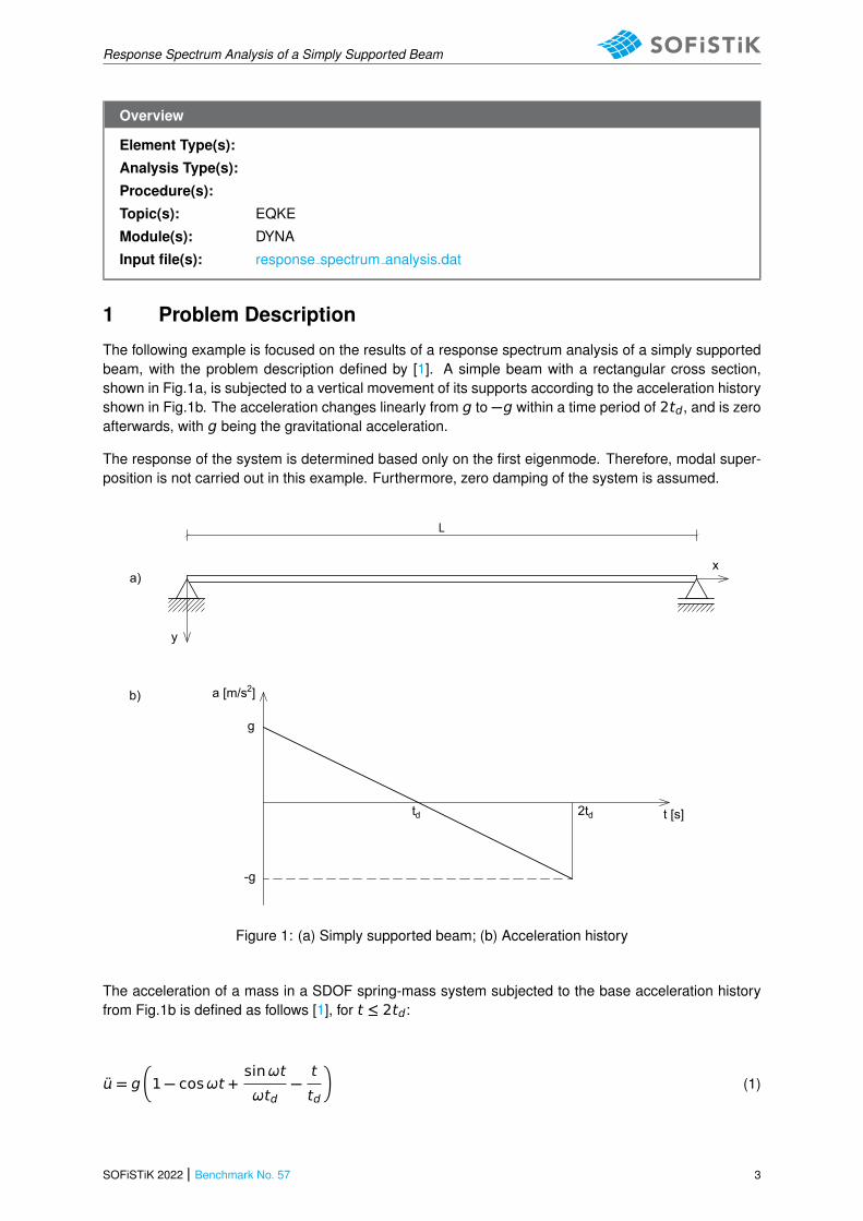
The following example is focused on the results of a response spectrum analysis of a simply supportedbeam, with the problem description defined by [1]. A simple beam with a rectangular cross section,shown in Fig.1a, is subjected to a vertical movement of its supports according to the acceleration historyshown in Fig.1b. The acceleration changes linearly from g to −g within a time period of 2td, and is zeroafterwards, with g being the gravitational acceleration.

The response of the system is determined based only on the first eigenmode. Therefore, modal super-position is not carried out in this example. Furthermore, zero damping of the system is assumed.

L

a)

b)

y

x

a [m/s2]

t [s]td 2td

g

-g

Figure 1: (a) Simply supported beam; (b) Acceleration history

The acceleration of a mass in a SDOF spring-mass system subjected to the base acceleration historyfrom Fig.1b is defined as follows [1], for t ≤ 2td:

= g�

1 − cosωt +sinωt

ωtd−

t

td

�

(1)

SOFiSTiK 2022 | Benchmark No. 57 3

Response Spectrum Analysis of a Simply Supported Beam

and for t > 2td:

= t=2td cosω(t − 2td) + t=2tdsinω(t − 2td)

ω(2)

where ω is the circular eigenfrequency.

2 Reference Solution

In the first step of the response spectrum analysis, the eigenfrequency of the first eigenmode is calcu-lated as follows [1]:

ƒ =π

22

√

√

√Ey

m(3)

where is the length and m is the mass per unit lenght of the beam, and Ey is the bending stiffness.

Based on the calculated eigenfrequency, the maximum relative displacement of the equivalent SDOFsystem, m,0, is determined from the corresponding response spectrum [1]. Subsequently, the maxi-mum beam deflection is calculated [1]:

m = m,0 (4)

The shape function for the first eigenmode () is given by [1]

() = sinπ

(5)

, and the modal participation factor is calculated as:

=

∫

0m()d

∫

0m[()]2d

=4

π(6)

The bending moment is defined as follows [1]:

M = −Ey∂2()

∂2(7)

4 Benchmark No. 57 | SOFiSTiK 2022

Response Spectrum Analysis of a Simply Supported Beam

where () is the beam deflection for the first eigenmode

() = m sinπ

(8)

Therefore, the maximum bending moment in the middle of the span is computed as:

My,m =Eyπ2

2m (9)

3 Model and Results

Material, geometry and loading properties of the beam model defined in a plane system are summarizedin Table 1.

Table 1: Model Properties

Material Properties Geometric Properties Loading

E = 206842MP = 6.096m g = 10m/s2

ρ = 104730 kg/m3 h = 35.56mm td = 0.1 s

b = 3.7026mm

The response spectrum values are calculated as maximum acceleration values, in the units of g, fromthe Equations 1 and 2 as a function of the eigenperiod. For the purpose of this example, only the valuesin the proximity of the system´s first eigenperiod are taken as the input points of the response spectrum.The selected points are listed in Table 2 and also shown on the graph of the response spectrum, whichis plotted as a function of the eigenfrequency in Figure 2.

Table 2: Calculated points of the response spectrum

Eigenfrequency [Hz] Eigenperiod [s] Max. acceleration [g]

5.00 0.20 2.000000

5.50 0.181818 1.818181

6.00 0.166667 1.666667

6.05 0.165289 1.652893

6.10 0.163934 1.639344

6.15 0.162602 1.626016

6.50 0.1538461 1.538461

7.00 0.142857 1.428571

SOFiSTiK 2022 | Benchmark No. 57 5

Response Spectrum Analysis of a Simply Supported Beam

0 1 2 3 4 5 6 7 8 9 10 110

0.2

0.4

0.6

0.8

1

1.2

1.4

1.6

1.8

2

2.2

Eigenfrequency ƒ [Hz]

Max

imum

acce

lera

tion

resp

onse

[m/s2]

Figure 2: The response spectrum and the selected input points

The calculated values of the eigenfrequency ƒ of the first mode, and the maximum deflection m andthe bending moment My,m in the middle of the span as a result of the response spectrum analysis,are compared with the reference values in Table 3.

Table 3: Results

SOF. Ref. [1]

ƒ [Hz] 6.12 6.10

m [mm] 14.15 14.22

My,m [kNm] 108.03 108.41

4 Conclusion

A very good agreement between the reference solution and the numerical results calculated bySOFiSTiK verifies the implementation of the response spectrum analysis.

5 Literature

[1] J.M. Biggs. Structural Dynamics. McGraw-Hill, 1964.

6 Benchmark No. 57 | SOFiSTiK 2022