Response of maize and olive to climate change...
179
UNIVERSIDAD POLITÉCNICA DE MADRID ESCUELA TÉCNICA SUPERIOR DE INGENIEROS AGRONÓMOS DEPARTAMENTO DE PRODUCCIÓN AGRARIA Response of maize and olive to climate change under the semi-arid conditions of southern Spain Tesis doctoral CLARA GABALDÓN LEAL Ingeniera Agrónoma 2016
Transcript of Response of maize and olive to climate change...

UNIVERSIDAD POLITÉCNICA DE MADRID
ESCUELA TÉCNICA SUPERIOR DE INGENIEROS AGRONÓMOS
DEPARTAMENTO DE PRODUCCIÓN AGRARIA
Response of maize and olive to climate change under the semi-arid conditions of
southern Spain
Tesis doctoral
CLARA GABALDÓN LEAL
Ingeniera Agrónoma
2016


DEPARTAMENTO DE PRODUCCIÓN AGRARIA
ESCUELA TÉCNICA SUPERIOR DE INGENIEROS AGRÓNOMOS
UNIVERSIDAD POLITÉCNICA DE MADRID
Response of maize and olive to climate change under the semi-arid conditions of
southern Spain
TESIS DOCTORAL
Clara Gabaldón Leal Ingeniera Agrónoma
DIRECTORES
Dr. Ignacio Lorite Torres. Doctor Ingeniero Agrónomo
Dra. Margarita Ruiz-Ramos. Doctora Ingeniera Agrónoma
2016


UNIVERSIDAD POLITÉCNICA DE MADRID
Tribunal nombrado por el Mgfco. y Excmo. Sr. Rector de la Universidad Politécnica
de Madrid, el día…………. de…………… de 2016.
Presidente:
Vocal:
Vocal:
Vocal:
Secretario:
Suplente:
Suplente:
Realizado el acto de defensa y lectura de la Tesis el día……. de………….. de 2016, en
la E.T.S.I. Agrónomos.
EL PRESIDENTE LOS VOCALES
EL SECRETARIO


ACKNOWLEDGEMENTS
En primer lugar, quiero agradecer a mis dos directores de Tesis, Dra. Margarita
Ruiz-Ramos y Dr. Ignacio Lorite Torres, por darme la oportunidad de realizar este
trabajo, por sus enseñanzas, su paciencia y por ayudarme a conseguir que este
documento llegue a buen puerto. Gracias también por darme la oportunidad de asistir
a congresos que me han abierto puertas y me han dado más seguridad en mi misma.
Al Dr Jon Lizaso por estar siempre disponible para mis preguntas sobre el maíz y
los modelos de cultivo. También quiero agradecer a la Dra. Heidi Webber, al Dr.
Thomas Gaiser y al Dr. Frank Ewert por acogerme en la Universidad de Bonn, por
facilitarme trabajar con ellos, gracias por su valiosa colaboración en parte de esta tesis.
A Alfredo, por su ayuda con el Matlab, gracias por tu paciencia. Asimismo quiero
agradecer a todos los coautores de los artículos incluidos en esta Tesis y cuyos
nombres figuran en la primera página de cada capítulo, muchas gracias por vuestros
valiosos comentarios y aportaciones.
Quiero agradecer a todos mis compañeros tanto de la Universidad de Madrid,
Alba, Maria S., Maria, Espe, Mirian, Omar, Juan y Javi como del IFAPA de Córdoba,
Cristina S., María, Nestor y en especial a mi compañero de despacho Juanmi, y como
no a todos mis compañeros de Córdoba por acogerme y apoyarme desde el primer día
que llegue. Pedro, Ana, Juanma, Belén, Fran, Pepe, sin vosotros este trabajo hubiera
sido mucho más difícil.
A Miguel Zamora, por enseñarme tanto sobre el maíz y el campo, por sacarme
siempre una sonrisa bajo los más de 40 grados del julio Cordobés.
A Cris y a Olga porque amigas como vosotras hacen que todo sea más fácil,
aunque vivamos lejos os he sentido muy cerca en este proceso, gracias también a
vosotras.
A mi familia, gracias a mis padres y a mi hermano por su apoyo incondicional.
Gracias a Josu, sin ti esto no hubiera sido posible, gracias por animarme siempre a
seguir, por apoyarme incansablemente, esta recta final ha sido mucho más fácil a tu
lado. Gracias
A todos vosotros, Muchas Gracias


INDEX
INDEX
ABBREVIATIONS ..................................................................................................................i
SUMMARY.......................................................................................................................... v
RESUMEN .......................................................................................................................... ix
INTRODUCTION ................................................................................................................. 1
OBJECTIVES ..................................................................................................................... 13
THESIS STRUCTURE ......................................................................................................... 15
CHAPTER 1. STRATEGIES FOR ADAPTING MAIZE TO CLIMATE CHANGE AND EXTREME
TEMPERATURES IN ANDALUSIA, SPAIN .......................................................................... 17
ABSTRACT .................................................................................................................... 19
1.1. INTRODUCTION ................................................................................................ 20
1.2. MATERIAL AND METHODS ............................................................................... 22
1.2.1. Location ........................................................................................................ 22
1.2.2. Climate data ................................................................................................. 23
1.2.3. Crop modelling ............................................................................................. 26
1.2.4. Extreme events ............................................................................................. 28
1.3. RESULTS ............................................................................................................ 29
1.3.1. Crop model calibration and validation ......................................................... 29
1.3.2. Evaluation under the present climate .......................................................... 29
1.3.3. Impact and adaptation projections .............................................................. 30
1.3.4. Extreme events ............................................................................................. 36
1.4. DISCUSSION ...................................................................................................... 37
1.4.1. Impacts ......................................................................................................... 37
1.4.2. Agronomic adaptations ................................................................................ 38
1.4.3. Extreme Tmax events ................................................................................... 40
1.5. CONCLUSIONS .................................................................................................. 40
CHAPTER 2. MODELLING THE IMPACT OF HEAT STRESS ON MAIZE YIELD FORMATION 43
ABSTRACT .................................................................................................................... 45
2.1. INTRODUCTION ................................................................................................ 46

INDEX
2.2. MATERIAL AND METHODS ............................................................................... 49
2.2.1. Experimental data ........................................................................................ 49
2.2.1.1. Argentine experiments ............................................................................. 49
2.2.1.2. Spanish experiments ................................................................................. 50
2.2.2. Model description ......................................................................................... 51
2.2.3. Simulation steps ........................................................................................... 53
2.3. RESULTS ............................................................................................................ 56
2.3.1. Step1: Determination of yield reduction heat stress factor ......................... 56
2.3.2. Step 2. Model calibration ............................................................................. 56
2.3.3. Step 3. Model evaluation ............................................................................. 60
2.4. DISCUSSION ...................................................................................................... 64
2.5. CONCLUSION .................................................................................................... 67
CHAPTER 3. IMPACT OF CHANGES IN MEAN AND EXTREME TEMPERATURES CAUSED BY
CLIMATE CHANGE ON OLIVE FLOWERING AT SOUTHERN SPAIN ................................... 69
ABSTRACT .................................................................................................................... 71
3.1. INTRODUCTION ................................................................................................ 72
3.2. MATERIAL AND METHODS ............................................................................... 75
3.2.1. Study area .................................................................................................... 75
3.2.2. Experimental design and measurements ..................................................... 76
3.2.3. Baseline and projected climate for southern Spain ..................................... 77
3.2.4. Approaches for flowering date estimation .................................................. 79
3.2.5. Evaluation of olive vulnerability to extreme events ..................................... 82
3.3. RESULTS ............................................................................................................ 83
3.3.1. Observed phenological behavior for olive crop under baseline and future
climate conditions ....................................................................................................... 83
3.3.2. Performance of phenological model parameters under baseline and future
climate conditions ....................................................................................................... 84
3.3.3. Projections of future flowering dates ........................................................... 85
3.3.4. Extreme temperature events ........................................................................ 89
3.3.5. Vulnerability and alternative suitable areas for olive cultivation at southern
Spain ……………………………………………………………………………………………………………… 94
3.4. DISCUSSION ...................................................................................................... 95

INDEX
3.5. CONCLUSION .................................................................................................. 100
GENERAL DISCUSSION .................................................................................................. 103
GENERAL CONCLUSIONS ............................................................................................... 111
GENERAL REFERENCES .................................................................................................. 115
REFERENCES CHAPTER 1 ............................................................................................... 131
REFERENCES CHAPTER 2 ............................................................................................... 139
REFERENCES CHAPTER 3 ............................................................................................... 145
ANNEX .......................................................................................................................... 153


ABBREVIATIONS
i
ABBREVIATIONS
ADAT Anthesis date
ADPS Adaptation selected
AEMET Spanish meteorological agency
An Argentine experiment n
AOC Atlantic ocean coast
B Baseline period
C Control plots
CV Coefficient of variation
DAS Days after sowing
DJF Winter (December, January, February)
DOY Day of the year
DSSAT Decision Support System for Agrotechnology Transfer
DTmax Mean increment of maximum temperatures
DTmin Mean increment of minimum temperatures
EDO End of dormancy
ENS-EOBS 12 RCMs from the ENSEMBLES project with a bias correction in temperature and precipitation with respect to the E-OBS gridded observational dataset
ENS-Spain02 12 RCMs from the ENSEMBLES project with a bias correction in temperature and precipitation with respect to the Spain02 gridded observational dataset
E-OBS Gridded observational dataset (Haylock et al. 2008)
EPP Effective pollination period
ETc Crop evapotranspiration
FAO Food and Agriculture Organization
fdmgn Simulated attainable yield normalized by the maximum value
FF Far Future
fHS Fractional stress intensity index
Fobs-Forg Difference between flowering dates observed and estimated
FRTDM Fraction of aboveground biomass to be translocated to seeds
G2 Maximum possible number of kernels per plant
G3 Kernel filling rate during the linear grain-filling stage and under optimum conditions
GCM Global climate model
GDD Growing degree days
GDP Gross domestic product
GH Greenhouse
ABBREVIATIONS
ii
GSn Growing stage n
GV Guadalquivir Valley
H Heated plots
hs1d Heat stress events of one day above threshold
hs3d Heat stress events of three consecutive days above threshold
HSF Heat stress during flowering
IP Iberian Peninsula
IPCC Intergovernmental Panel on Climate Change
IRR Irrigation requirements
IWP Irrigation water productivity
JJA Summer (June, July, August)
LAD Leaf area duration
LAI Leaf area index
MAM Spring (May, April, May)
MBE Mean bias error
MDAT Maturity date
N North
NE Northeast
NF Near future
NW Northwest
Oi Observed value
OU Outdoors
p Dimensionless penalty constant
P1 Thermal time from seedling emergence to the end of the juvenile phase
P2 Extent to which development (expressed as days) is delayed for each hour increase in photoperiod above the longest photoperiod at which development proceeds at a maximum rate
P5 Thermal time from silking to physiological maturity
PAR Photosynthetically active radiation
PARi Intercepted PAR
PHINT Phylochron interval
PostS Post-silking treatment
Precip Precipitation
PreS Pre-silking treatment
RAEA Red Andaluza de Experimentación Agraria
RCM Regional climate model
RCP Representative concentration pathways
RedHS Heat stress reduction factor
RGRLAI Maximum relative increase in LAI
RIA Agroclimatic Information Network of Andalusia

ABBREVIATIONS
iii
RMSE Root mean square error
RTMCO Correction factor for RUE
RUE Radiation use efficiency
Si Simulated value
S South
SE Southeast
SIMPLACE <Lintul5,HS,Tc>
Combined model SIMPLACE<Lintul5, DRUNIR, CanopyT, HeatStressHourly>
SLA Specific leaf area
Sn Spanish experiment n
SON Autumn (September, October, November)
Spain02 Gridded observational dataset (Herrera et al., 2012)
SRAD Solar radiation
SRES Special Report on Emission Scenarios
Tair Air temperature
Tair_ear Air temperature at ear level
Tair_tas Air temperature at tassel level
Tb Base temperature
Tcan Canopy temperature
Tcan,lower Tcan lower limit
Tcan,upper Tcan upper limit
Tcrit Critical temperature
Tday Daytime
Th Hourly temperature
Tlim Limit temperature for chilling accumulation
Tmax Maximum temperature
Tmean Mean temperature
Tmin Minimum temperature
To Optimal temperature
TSUM1 Thermal time from emergence to anthesis
TSUM2 Thermal time from anthesis to maturity
TT Thermal time
TThs Hourly stress thermal time
TTorg Thermal time (from De Melo-Abreu et al., 2004)
TU Total chilling units
TUE Transpiration use efficiency
TUmax Maximum value chilling units
TUmean Mean value chilling units
TUmin Minimum value chilling units

ABBREVIATIONS
iv
TUorg Chilling units (from De Melo-Abreu et al., 2004)
TWP Total water productivity
Tx Breakpoint temperature
Y Maize grain yield
Yn Normalized Y
SUMMARY
v
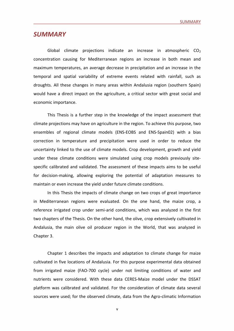
SUMMARY
Global climate projections indicate an increase in atmospheric CO2
concentration causing for Mediterranean regions an increase in both mean and
maximum temperatures, an average decrease in precipitation and an increase in the
temporal and spatial variability of extreme events related with rainfall, such as
droughts. All these changes in many areas within Andalusia region (southern Spain)
would have a direct impact on the agriculture, a critical sector with great social and
economic importance.
This Thesis is a further step in the knowledge of the impact assessment that
climate projections may have on agriculture in the region. To achieve this purpose, two
ensembles of regional climate models (ENS-EOBS and ENS-Spain02) with a bias
correction in temperature and precipitation were used in order to reduce the
uncertainty linked to the use of climate models. Crop development, growth and yield
under these climate conditions were simulated using crop models previously site-
specific calibrated and validated. The assessment of these impacts aims to be useful
for decision-making, allowing exploring the potential of adaptation measures to
maintain or even increase the yield under future climate conditions.
In this Thesis the impacts of climate change on two crops of great importance
in Mediterranean regions were evaluated. On the one hand, the maize crop, a
reference irrigated crop under semi-arid conditions, which was analyzed in the first
two chapters of the Thesis. On the other hand, the olive, crop extensively cultivated in
Andalusia, the main olive oil producer region in the World, that was analyzed in
Chapter 3.
Chapter 1 describes the impacts and adaptation to climate change for maize
cultivated in five locations of Andalusia. For this purpose experimental data obtained
from irrigated maize (FAO-700 cycle) under not limiting conditions of water and
nutrients were considered. With these data CERES-Maize model under the DSSAT
platform was calibrated and validated. For the consideration of climate data several
sources were used; for the observed climate, data from the Agro-climatic Information

SUMMARY
vi
Network of Andalusia (RIA) was used and for the simulated climate, data from an
ensemble of twelve regional models (ENS-EOBS) with a bias correction in temperature
and precipitation over the original European project ENSEMBLES was used.
The results for the end of the 21st century project a reduction in the maize crop
cycle length causing a decrease in the duration of the grain filling period and then, a
decrease in yield maize and irrigation requirements. In addition, the stomatal closure
caused by the increase in CO2 concentration, could lead to an increase in the water use
efficiency. To reduce the negative impacts on maize crop, in this Thesis some
adaptation measures were evaluated. Thus, some proposed adaptations were to
advance the sowing date 30 days earlier than current and to change the maize cultivar
seeking to increase the grain filling period and its efficiency. These adaptations offset
the yield losses and even in some cases, the projected yield was increased. The
impacts and the adaptation strategies effect were also evaluated from the point of
view of the incidence of extreme temperature events at flowering, showing an
increase in the number of extreme events as well as in the production damage at the
end of the 21st century. The proposed adaptation strategies previously described
resulted in an overall reduction of crop damage by extreme maximum temperatures at
all locations with the exception of specific locations such as Granada, where losses
were limited to 8 %.
With this precedent, the Chapter 2 deals with the modelling of heat stress
events on maize yield. A heat stress response function was developed and evaluated
into the modeling framework SIMPLACE, within the Lintul5 crop model and the canopy
temperature model (CanopyT). For this task, experimental data from Pergamino
(Argentina) considering a maize temperate hybrid, and from Lleida (Spain), with a
maize cultivar FAO-700 cycle, were used. In both experiments the maize plants were
subjected to high temperature conditions around flowering by placing polyethylene
tents. Argentine data were used to obtain a yield reduction factor in relation with
thermal time under a critical temperature of 34 °C during the flowering period. On the
other hand, the Spanish data were divided into two sets, one of them under control

SUMMARY
vii
conditions to calibrate the model, and the other set to validate it using the reduction
factor obtained from the Argentina data. The model evaluated consider canopy
temperature (Tcan) or air temperature (Tair) for the simulation of impact of heat events
on maize yield, obtaining better model performance using Tcan when the critical
temperature was set to 34 °C. However, when critical temperature for Tair was
increased to 39 °C, the results were similar for both temperatures (canopy and air)
indicating that for irrigated and high radiation conditions the air temperature could be
used as input in the model without the need to simulate the canopy temperature.
The Chapter 3 evaluates the impacts of climate change on olive flowering for
current and future climate conditions at southern Spain. For this purpose an
experiment located at Cordoba from 1st October 2013 to the end of May 2014 was set
to evaluate ten olive genotypes under two different climate conditions, one outdoors
(OU) and the other inside of a greenhouse (GH). The aim of the experiments carried
out in GH was to identify the impacts of the increase in temperatures on olive
phenology, reproducing the mean increment of maximum and minimum temperatures
(DTmax, DTmin) projected at the end of the 21st century. To quantify these increases,
data from an ensemble of twelve regional climate models (ENS-Spain02), with a bias
correction in temperature and precipitation from the original climate models of the
ENSEMBLES European project were used. Once the foreseen climate conditions were
reproduced in GH, olive flowering dates were evaluated under both climate conditions
using previous flowering models, obtaining good results under OU conditions, but not
for GH. Based on these results, a new model was proposed and evaluated taken into
account on one hand the chilling hour accumulation and on the other hand obtaining
the flowering dates achieved after heating accumulation. Once the new model was
developed, flowering dates were evaluated for the whole region of Andalusia,
obtaining a mean advance in the flowering date of 17 days for all the genotypes for the
climate conditions foreseen at the end of the 21st century. A spatial analysis of the
results was carried out, identifying the highest advance in flowering date in the
mountainous area of Jaen and Granada provinces and the lowest in the Atlantic Ocean
Coast area. Finally, a spatial analysis evaluating the vulnerable and suitable areas for

SUMMARY
viii
olive cultivation in Andalusia at the end of the 21st century was held. Thus, several
areas were vulnerable due to high temperatures in flowering (North and Northeast
regions) or to lack of chilling hour accumulation in winter (Atlantic Ocean and the
Southeast coast). Equally, potential new areas for olive cultivation were detected as
the southern area of Andalusia.

RESUMEN
ix
RESUMEN
Las proyecciones climáticas globales indican un aumento en la concentración de
CO2 atmosférico que, para las regiones mediterráneas, implican un aumento tanto en las
temperaturas medias como en las máximas, una disminución promedio de las
precipitaciones y un aumento de la variabilidad temporal y espacial de los fenómenos
extremos relacionados tanto con la lluvia como con las sequías. Todos estos cambios
tendrían un impacto directo en la agricultura de muchas áreas de la región de Andalucía
(sur de España), sector crítico de gran importancia social y económica.
Esta tesis es un paso más en el conocimiento de la evaluación de impactos que
las proyecciones climáticas pueden tener sobre la agricultura en la región. Para lograr
este propósito, se han utilizado dos conjuntos de modelos climáticos regionales (ENS-
EOBS y ENS-Spain02) con una corrección del sesgo de la temperatura y la precipitación
con el fin de reducir la incertidumbre relacionada con el uso de modelos climáticos. El
desarrollo del cultivo, crecimiento y rendimiento en estas condiciones climáticas se han
simulado utilizando modelos de cultivos previamente calibrados y validados localmente.
La evaluación de estos impactos pretende ser útil para la toma de decisiones, lo que
permite explorar el potencial de las medidas de adaptación para mantener o incluso
aumentar el rendimiento bajo condiciones climáticas futuras.
En esta Tesis han evaluado los efectos del cambio climático en dos cultivos de
gran importancia en las regiones mediterráneas. Por un lado, el maíz, un cultivo en
regadío de referencia en condiciones semiáridas, analizado en los dos primeros capítulos
de la tesis. Por otro lado, el olivo, ampliamente cultivado en Andalucía, siendo la
principal región productora de aceite de oliva a nivel mundial; este cultivo se analiza en
el Capítulo 3.
El Capítulo 1 se describe los impactos y adaptaciones al cambio climático para el
maíz cultivado en cinco localizaciones de Andalucía. Para este fin se han utilizado datos
experimentales obtenidos a partir de maíz en regadío (ciclo FAO-700) bajo condiciones
no limitantes de agua y nutrientes. Con estos datos el modelo CERES-Maize bajo la

RESUMEN
x
plataforma DSSAT se ha calibrado y validado. Los datos climáticos considerados en este
estudio proceden de varias fuentes; para el clima observado, se han utilizado los datos
de la Red de Información Agro-climáticas de Andalucía (RIA), y para el clima simulado,
los datos de un conjunto de doce modelos regionales (ENS-EOBS) con una corrección del
sesgo en la temperatura y la precipitación sobre los modelos originales del proyecto
Europeo ENSEMBLES.
Los resultados obtenidos para el final del siglo XXI proyectan una reducción en la
longitud del ciclo del maíz causando una disminución en la duración del periodo de
llenado de grano y, por tanto, una disminución del rendimiento del maíz y de las
necesidades de riego. Además, el cierre estomático causado por el aumento de la
concentración de CO2, podría conducir a un aumento en la eficiencia del uso del agua.
Para reducir los impactos negativos sobre el cultivo de maíz, en esta Tesis se evalúan
algunas medidas de adaptación. De este modo, algunas adaptaciones propuestas son el
adelanto de la fecha de siembra 30 días antes de la fecha actual y el cambio de la
variedad de maíz buscando aumentar la eficiencia y período de llenado del grano.. Estas
adaptaciones compensan las pérdidas de rendimiento e incluso en algunos casos, las
proyecciones indican un aumento del rendimiento. Los impactos y el efecto estrategias
de adaptación también se han evaluado desde el punto de vista de la incidencia de
eventos extremos de temperatura en la floración, mostrando un aumento en el número
de eventos extremos, así como en el daño en la producción a finales del siglo XXI. Las
estrategias de adaptación propuestas descritas anteriormente dieron lugar a una
reducción en los daños por temperaturas máximas extremas en todos los lugares, con la
excepción de zonas específicas, como Granada, donde las pérdidas se limitan al 8 %.
Una vez identificado el problema en el Capítulo 1, una vía de solución se plantea
en el Capítulo 2, que trata la modelización de eventos de estrés térmico en el
rendimiento del maíz. Una función de respuesta al estrés térmico fue desarrollado y
evaluado en el marco de modelado SIMPLACE, dentro del modelo de cultivo Lintul5 y de
un modelo de temperatura de la cubierta (CanopyT). Para este cometido se han utilizado
datos experimentales de Pergamino (Argentina) considerando un híbrido templado
maíz, y de Lleida (España), con un ciclo de cultivo de maíz FAO-700. En ambos

RESUMEN
xi
experimentos las plantas de maíz fueron sometidas a condiciones de alta temperatura
alrededor de la floración mediante la colocación de tiendas de polietileno. Los datos de
Argentina se han utilizado para obtener un factor de reducción de rendimiento en
relación con el tiempo térmico durante el periodo de floración considerando una
temperatura crítica de 34 °C. Por otra parte, los datos de España se dividieron en dos
grupos, uno de ellos en condiciones de control para calibrar el modelo, y el otro
conjunto para validarlo usando el factor de reducción obtenido a partir de los datos de
Argentina. El modelo evaluado considera la temperatura de cubierta (Tcan) o la
temperatura del aire (Tair) para la simulación del impacto de los eventos de calor sobre el
rendimiento del maíz, obteniendo un mejor resultado utilizando Tcan cuando la
temperatura crítica se fijó en 34 °C. Sin embargo, cuando la temperatura crítica para Tair
se aumentó a 39 °C, los resultados fueron similares para ambas temperaturas (cubierta y
aire) que indican que para las condiciones de riego y alta radiación la temperatura del
aire se podría utilizar como dato de entrada en el modelo sin necesidad de simular la
temperatura de la cubierta.
El Capítulo 3 evalúa los impactos del cambio climático en la floración del olivo
para las condiciones climáticas actuales y futuras en el sur de España. Para este
propósito se ha llevado a cabo un experimento en la localidad de Córdoba desde el 1 de
Octubre 2013 hasta finales de Mayo 2014 en el que se han evaluado diez genotipos de
olivo en dos condiciones climáticas diferentes, uno en el exterior (OU) y el otro en el
interior de un invernadero (GH). El objetivo de los experimentos llevados a cabo en GH
fue identificar los impactos del aumento de las temperaturas en la fenología del olivo,
reproduciendo el incremento medio de las temperaturas máximas y mínimas (DTmax,
DTmin) proyectados al final del siglo XXI. Para cuantificar estos aumentos, se han
utilizado los datos de un conjunto de doce modelos climáticos regionales (ENS-Spain02),
con una corrección en el sesgo de la temperatura y la precipitación de los modelos
climáticos sobre los originales del proyecto Europeo ENSEMBLES. Una vez que las
condiciones climáticas previstas fueron reproducidas en GH, las fechas de floración del
olivo han sido evaluadas bajo las dos condiciones climáticas usando modelos de
floración anteriores, obteniendo buenos resultados en condiciones OU, pero no para
GH. Basándose en estos resultados, se ha propuesto y evaluado un nuevo modelo

RESUMEN
xii
teniendo cuenta por un lado la acumulación frío y por otra parte el cálculo de las fechas
de floración después de un periodo de acumulación por calor. Una vez desarrollado el
nuevo modelo, se han evaluado las fechas de floración para toda la región de Andalucía,
obteniendo un adelanto medio en la fecha de floración de 17 días para todos los
genotipos bajo las condiciones climatológicas previstas al final del siglo XXI. Finalmente
se realizó un análisis espacial de los resultados, identificando el mayor adelanto en la
fecha de floración en las zonas montañosas de las provincias de Jaén y Granada y la
menor en la costa del océano Atlántico. Igualmente, se ha realizado un análisis espacial
evaluando las áreas vulnerables y adecuadas para el cultivo del olivo en Andalucía a
finales del siglo XXI. De este modo, varias zonas muestran vulnerables a las altas
temperaturas en floración (regiones Norte y Nordeste) o por falta de acumulación de
frío en invierno (costa del Océano Atlántico y la costa sureste). Igualmente, se han
identificado nuevas áreas potenciales para el cultivo del olivo como la zona sur de
Andalucía.

INTRODUCTION
1
INTRODUCTION
Agriculture is one of the most important social and economic activity at global
scale, and directly dependent on the climate and edaphic conditions, making this activity
high vulnerable to climate change effects (Olesen and Bindi, 2002; Easterling et al., 2007;
Tubiello and Fischer, 2007). This Thesis has been developed in Andalusia, located in the
South of Spain, and is focused on the impact of climate change in two representative
crops of the region: maize (Zea mays) and olive (Olea europaea). Maize is a summer crop
that is the world’s most widely grown cereal in terms of grain production, although
wheat and rice are the most important for direct human consumption and cultivated
area (Steduto et al., 2012). Maize crop is cultivated in a wide range of climate and soil
conditions, and can be considered as a reference herbaceous irrigated crop of the
Andalusian cropping systems. In Andalusia, maize is irrigated and accounted for a mean
cultivated area of around 34.000 ha and 11.000 kg ha-1 production for the period 2010-
2013 (RAEA, 2015). Olive is a traditional Mediterranean crop, being Spain the first olive
oil producer in the world with around 40 % of the total production (FAOSTAT, 2016). The
southern Spanish region of Andalusia represents the first national olive oil producer with
80% of the national production (1.1M tons; CAPDR, 2016a, covering 1.4 Mha which
around 33 % correspond to irrigated olives (MAGRAMA, 2015). Olive is recognized by its
social role as this crop generates a high rate of employment per surface unit and
currently provides around 32 % of total agriculture employees in Andalusia region
(CAPDR, 2008).
According to the World Meteorological Organization (WMO), climate change
refers to a statistically significant variation in either the mean state of the climate or in
its variability, persisting for an extended period (typically decades or longer).
Furthermore, the United Nations Framework Convention on Climate Change (UNFCCC)
provides another definition, where the “climate change refers to a change of climate
that is attributed directly or indirectly to human activity that alters the composition of
the global atmosphere and that is in addition to natural climate variability observed over
comparable time periods”. Therefore, both definitions are different, as the anthropic
attribution of the change is not part of the WMO definition.

INTRODUCTION
2
Historical observational atmospheric data until date show a significant increase in
the greenhouse gases concentration (Fig I.1). This trend is projected to continue, causing
an increase in global temperature at the end of the 21st century (Intergovernmental
Panel on Climate Change, IPCC, 2014). The changes in mean precipitation will not be
uniform: an increase is projected in the high latitudes, mid-latitudes wet regions and
equatorial Pacific while in many mid latitude as southern Europe and subtropical dry
regions precipitation will likely decrease (IPCC, 2014).
Figure I.1. Past atmospheric concentrations of the greenhouse gases carbon dioxide (CO2, green), methane (CH4, orange) and nitrous oxide (N2O, red) determined from ice core data (dots) and from direct atmospheric measurements (lines). Concentration units are parts per million (ppm) or parts per billion (ppb) (source: IPCC, 2014)
In order to simulate the foreseen changes in the climate conditions and based on
the current information, the generation of climate projections implies a successive
decision steps. One of these steps is the selection of emission scenarios, for instance
among the SRES scenarios (Special Report on Emission Scenarios, Nakićenović et al.,
2000), which describe the driving forces of future emissions. SRES scenarios follow four
storylines grouped into four scenario families: A1, A2, B1 and B2. Group A1 describes a
world in development with rapid economic growth and a reduction of regional
differences. This group is disaggregated in three scenarios according to the base of the
technological development: fossil fuels (A1F), non-fossil (A1T) or balanced (A1B).
Scenario A2 describes a very heterogeneous world, determined by self-reliance and
preservation of local identities, while the B1 describes a convergent world population
that reaches a maximum and then decreases. Finally the B2 scenario describes a world
with an increased concern for environmental and social sustainability compared to the
A2 scenario. Until recently, climate projections have been given only using these

INTRODUCTION
3
emission scenarios; however, there are currently a new generation of proposed
scenarios, the Representative Concentration Pathways (RCPs; Moss et al., 2010), taking
into account also the system resilience and mitigation and adaptation strategies. These
RCPs have been considered in the last IPCC report (IPCC, 2014).
Simulated climate under climate scenarios is produced by Global Climate Models
(GCMs). These models cover the entire globe with a resolution ranging from 150 x 150
km to 300 x 300 km and describe the climate behavior by integrating different ocean-
atmospheric dynamics with mathematical equations to generate climate projections.
There are two main downscaling techniques for the generation of climate projections at
regional level providing climate information on a scale compatible with the regional and
local impact studies, the dynamic and the statistical methods. The dynamic downscaling
approach reduces the scale of the GCM outputs through the Regional Climate Model
(RCM) maintaining their boundary conditions; therefore the generated RCM are
numerical models run in a limited area nested in a GCM (Castro et al., 2005). The current
RCMs provide a resolution between 50 x 50 km and 5 x 5 km. In the other hand,
statistical downscaling techniques use transfer functions to represent the observed,
historical relationships between large-scale atmospheric variables with those observed
locally (Wilby et al., 1998).
This Thesis uses the first approach based on RCMs. RCMs consider the altitudinal
variation by including the topographic forcing in the atmospheric variability (Castro et
al., 2005), which is essential in the evaluation of climate change impacts on agriculture
in heterogeneous regions as Andalusia (Guereña et al., 2001). In spite of the use of RCMs
with high spatial resolution, climate projections contain multiple sources of uncertainty
such as the selection of emission scenarios, the driver GCM or the inherent uncertainty
to the climate model, as the different physical parameterization of models and their
resolution (Olesen et al., 2007; Ruiz-Ramos and Mínguez, 2010; Osborne et al., 2013).
Furthermore, RCMs simulations may present large biases when compared to
observations (Dosio and Paruolo, 2011; Ceglar and Kajfež-Bogataj, 2012) that can limit
their application at local and regional scale. For example, several studies indicate that
the simulated summer temperature at southern Europe of recent decades is
overestimated by RCMs (Christensen et al., 2008; Dosio et al., 2012). Another example is
given by Ceglar and Kajfež-Bogataj (2012), who showed that the use of raw simulations

INTRODUCTION
4
from RCMs into a crop model produces unrealistic maize yield estimations due to the
underestimation of the intensity of daily precipitation. This uncertainty could be reduced
with the bias correction of climate projections (Dosio et al., 2012; Ruiz-Ramos et al.,
2015). But it is noteworthy that the uncertainties in regional climate projections can be
better characterized and reduced when an ensemble of simulations exploring all the
relevant uncertainty dimensions is considered (Giorgi et al., 2009). For that reason, in
this Thesis an ensemble of climate projections from one of the major projects that has
generated regional projections for Europe, ENSEMBLES (www.ensembles-eu.org, Van
der Linden and Mitchell 2009), is used. The ENSEMBLES projections were still referred to
SRES scenarios and do not consider RCPs.
Most of the climate projections obtained with these climate models foresee a
global increase in mean temperature around 1 to 4 °C considering the range of RCPs
emissions scenarios by the end of the 21st century (IPCC, 2014), similar to the increase
provided by the previous IPCC report (IPCC, 2007). Temperature projections over Europe
(A1B scenario) show increases in the mean annual temperature, this increase being
higher in the summer months. Regarding precipitation, increases in northern Europe (up
to 16 %) and decreases in the South (from -4 to -24 %) are projected with high
uncertainty (Christensen et al., 2007; Bindi and Olesen, 2011) (Fig.I.2). Climate change
will also strongly impact on the frequency and intensity of extreme events (Easterling et
al., 2000; Sánchez et al., 2004; Beniston et al., 2007), this has been already observed, as
in the summer heat wave of 2003 and 2010 (Schär and Jendritzky, 2004; Barriopedro et
al., 2011). Extreme maximum temperature events (Meehl and Tebaldi, 2004; Hertig et
al., 2010) are projected to become more frequent in the future (Beniston, 2004; Schär
and Jendritzky, 2004; Tebaldi et al., 2006; Beniston et al., 2007; van der Velde et al.,
2012).

INTRODUCTION
5
Figure I.2 Temperature and precipitation changes over Europe for the A1B scenario. Top row, Annual mean, DJF and JJA temperature change between 1980 and 1999 and 2080 to 2099, averaged over 21 models. Bottom row, same as top, but for percentage of change in precipitation (from Christensen et al., 2007 and Bindi and Olesen, 2011).
The Mediterranean region is expected to be one of the most affected areas by
climate change (Giorgi and Lionello, 2008). In Spain, some temperature projections from
GCMs indicate an increase of around 4 °C during the warmest months considering both
A2 and B2 scenarios (Giannakopoulos et al., 2009). These results are in agreement with
Gosling et al. (2011) through the Met Office report for Spain, which projects an increase
in annual temperature up to around 4 °C for A1B scenario. Within the CMIP3 multi-
model ensemble of GCMs, made up of 21 members, the highest agreement between
models was found in the southern Spain when comparing the increase of the mean
annual temperature by 2100 with regard to the baseline climate (1960-1990). Also,
these authors report projections of rainfall decrease for the Southwest of Spain over 20
%, and between 10 and 20 % over other rest of the country. Van der Linden and Mitchel
(2009) in the ENSEMBLES European project (A1B scenario), report projections of
increase in temperatures for southern of Spain from 2 °C in winter months to up to 5 °C
in summer months, with a decrease in precipitation from 15 % in winter months to 30 %
in summer months. In general, regional projections for ENSEMBLES project for A1B
scenario showed the same trends that those of the former project PRUDENCE for A2, B2
scenarios (Christensen and Christensen, 2007) but the magnitudes of projected changes
are larger.

INTRODUCTION
6
Future projections of the impact of climate change on crops are usually obtained
through crop models combined with climate change scenarios. Crop models simulate
crop growth, phenology, development and production once calibrated and validated,
using mathematical representations of the main processes involved with different
degree of complexity and biophysical understanding. Crop models are commonly
classified into empirical or mechanistic (Dent and Blackie, 1979; Connolly, 1998;
Thornley and France, 2007). In one hand, empirical models apply functions fitted to data
without considering true simulations of the physiological processes involved in growth
(Fourcaud et al., 2008). In the other hand, the mechanistic models represent the
physiological responses of the crops to environmental variables and management to
estimate crop development, growth and yield.
Other way to classify the crop models is attending the way that the model
estimates the daily biomass accumulation under potential conditions; for instance the
carbon driven group, when the model is based on the carbon assimilation by leaves
through the photosynthesis process. Simulated growth processes and phenological
development are regulated by temperature, radiation, and atmospheric CO2
concentration and are limited by water availability (Todorovic et al., 2009); within this
kind of crop models we can find the WOFOST (Diepen et al., 1989; Boogaard et al., 1998)
and CROPGRO (Boote et al., 1998) models. The second group is the radiation driven
models, which simulate the biomass through the intercepted radiation using the
radiation use efficiency (RUE), as the models used in this Thesis: CERES-Maize (Jones and
Kiniry, 1986) and SIMPLACE (Gaiser et al., 2013). Finally, the third group, the water
driven models, uses the transpiration use efficiency (TUE) to calculate the biomass as
proportional to transpired water, as for instance, AQUACROP model (Raes et al., 2009;
Steduto et al., 2012).
Specifically for the crops addressed in this Thesis, maize growth and
development have been modeled through different procedures and several approaches
have been considered to achieve maize yield assessment. Thus, empirical functions
applied to grain yield, as GAEZ model (Fischer et al., 2002) or GLAM (Challinor et al.,
2004, 2005); considering daily increment in harvest index, as AQUACROP (Raes et al.,
2009; Steduto et al., 2012) or CROPSYST (Stockle et al., 2003; Moriondo et al., 2011); or

INTRODUCTION
7
determining grain number, as CERES-Maize (Jones and Kiniry, 1986) or APSIM maize
(Carberry et al., 1989).
The olive crop modelling has lower development than the maize one. To evaluate
the olive flowering dates, different models have been published based on the pollen
density (Galan et al., 2005; Bonofiglio et al., 2008; Oteros et al., 2014) or in phenological
observations (Orlandi et al., 2005). There are some models that calculate different
processes of the olive productivity, as the photosynthesis, transpiration or water use
efficiency (Diaz-Espejo et al., 2002, 2006; Connor and Fereres, 2005). Other models
calculate the biomass production based on annual radiation (Villalobos et al. 2006), the
functional approach based on the relation between yield and potential
evapotranspiration (Viola et al., 2012) or calculates the potential olive oil production
based on a three-dimensional model of canopy photosynthesis and respiration and the
dynamic distribution of assimilates among organs (Morales et al., 2016). However, there
is a need to improve the olive crop models under elevated both temperatures and CO2
concentrations (Moriondo et al., 2015).
To evaluate the impact of climate change on crops is essential to analyze each
component that affects crop growth, development and yield. Thus, components as
phenology, transpiration efficiency or harvest index play a critical role in the response to
crops to climate change. Phenology has been defined as the timing of recurring
biological events regarding to biotic (genetic background) and abiotic (environmental
and management) forces, and the interrelation among them (Lieth, 1974; Slafer et al.,
2009). It is noteworthy that the phenological phases are largely controlled by
temperature and day length (Sadras and Calderini, 2009). During the phenological period
of flowering, high temperatures affect the number of flowers per plant, limit the pollen
release and diminish the pollen viability, flower fertility and therefore the viable seeds
(Prasad et al., 2000, 2006; Wheeler et al., 2000; Moriondo et al., 2011; Vuletin Selak et
al., 2013). On the other hand, crop growth has been defined as an increase in the size of
an individual or organ with time and depends on the capture of resources including CO2,
radiation, water, N and other nutrients (Sugiyama, 1995; Sadras and Calderini, 2009).
Experiments under elevated CO2 concentration have shown that the carbon
uptake, growth and above-ground production increase, while specific leaf area and
stomatal conductance decrease (Ainsworth and Long, 2005) under these conditions.

INTRODUCTION
8
Those changes could benefit plants and especially C3 plants (olive), and both C3 and C4
under water stress conditions, due to the increase in water use efficiency (Vu and Allen,
2009; Allen et al., 2011). For herbaceous species, the C3 present more positive effect
than C4 species (maize) (Warrick et al., 1986). The trees are more responsive than
herbaceous species to elevated CO2 (Ainsworth and Long, 2005). There are few studies
dealing with olive trees under CO2 elevated concentrations, but the existing ones have
shown a positive response of the photosynthetic rate and a decreased stomatal
conductance, leading to greater water use efficiency with no effect on biomass
accumulation rate (Sebastiani et al., 2002; Tognetti et al., 2002). Therefore, in addition
to the effects of temperature and rainfall it is important to evaluate the effect of the
projected CO2 increase.
Maize grain yield is determined by the number of grains and its weight, being
largely dependent on the climate conditions during the critical period of flowering
(Fischer and Palmer, 1984; Kiniry and Ritchie, 1985; Grant et al., 1989; Lizaso et al.,
2007). During this period the grain number is determined (Fischer and Palmer, 1984;
Otegui and Bonhomme, 1998). Under high temperatures, the source capacity is reduced;
both the photosynthetic rate causing a reduction in the carbohydrates synthesis
(Barnabás et al., 2008) and the respiration rate (Wahid et al., 2007) are reduced. When
these net assimilation reductions occur during the critical period of flowering a
reduction in grain yield was observed (Andrade et al., 1999, 2002). Furthermore, the sink
capacity could be reduced under high temperatures due to low pollen viability (Herrero
and Johnson, 1980), grain abortion (Rattalino Edreira et al., 2011; Ordóñez et al., 2015)
or the synchrony disruption between anthesis and silking (Cicchino et al., 2010); this
reduction in sink capacity makes the losses of grain number irreversible. Large-scale
observational studies analyzing maize yields and temperature records indicate that large
yield losses are associated with even brief periods of high temperature when crop-
specific thresholds are surpassed (Schlenker and Roberts, 2009; Gourdji et al., 2013).
Regarding olive trees, pollen concentration studies have shown that the elevated
temperatures could generate an advance in the flowering date (Osborne et al., 2000;
Galán et al., 2005; Avolio et al., 2008; Orlandi et al., 2010), being this advancement an
indicator of the climate warming in the Mediterranean area (Osborne et al., 2000;
Moriondo et al., 2013). These higher temperatures and the heat stress events during

INTRODUCTION
9
flowering may cause damages such as ovarian abortion (Rallo, 1994), vegetative damage
(Mancuso and Azzarello, 2002) and pollen germination damage (Cuevas et al., 1994;
Koubouris et al., 2009), with the subsequent decrease in yield. Another important factor
to take into account is the projected water shortage. Thus, in spite of the olive drought
resistance (Connor and Fereres, 2005), the olive under water stress reduces the
photosynthetic rate due to the stomata closure (Fereres, 1984; Angelopoulos et al.,
1996). Another effect that can reduce yield appears when water stress during flowering
affect the fertilization, as the flowers remain closed (Rapoport et al., 2012). Also,
between the period from floral development to fruit development water stress has a
direct effect on fruit tissues (Rapoport et al., 2004; Gucci et al., 2009).
Observed phenological trends across Europe (1971-2000) for 542 plant species
indicate a mean advance 2.5 days per decade in leafing, flowering and fruiting records
(Menzel et al., 2006). Data since 1986 showed an advancement in foliation, flowering
and fruit ripening more evident in arboreal species (Olive, vine, Quercus spp.) than in
herbaceous ones, showing that the major factor in the earlier foliation, flowering and
fruit ripening was the increase in temperature (García-Mozo et al., 2010). In Cordoba, a
province located at southern Spain in Andalusia, an increase in mean temperature of 1
°C during March–April–May induced an advance in olive flowering of 7.6 days during the
1982-2007 (Orlandi et al., 2010).
Concerning the crop yield, French maize yields observed over the past 50-years
were found to decrease; this decrease has been related with an increase in the number
of days with maximum air temperature above 32 °C (Hawkins et al., 2013). Likewise, a
panel analysis for this species in the US determined that yields decreased with
cumulative degree days above 29 °C (Schlenker and Roberts, 2009). Furthermore, Lobell
et al., (2011) detected maize yield losses across Sub-Saharan Africa ranging from 1 to 1.7
% (depending on water availability) per each degree day above 30 °C.
Under climate change conditions, projected phenological trend across Europe
implies an advancement of the flowering and maturity dates of spring cereals of 1 to 3
weeks by 2040 (Olesen et al., 2012), partially explained by an advancement of sowing
dates. The projected rising temperatures in the spring and summer in the South of the
Iberian Peninsula would lead to a shortening of the cereal phenological cycles (Guereña

INTRODUCTION
10
et al., 2001), and in the case of the olive trees, a general advance of the crop cycle from
1 to 3 weeks could be expected at the end of the 21st century (Galan et al., 2005).
The projected effects on crop yield in Europe have been studied both at the
continental level (Olesen and Bindi, 2002, 2004; Bindi and Olesen, 2011), and at regional
level as well. In Mediterranean Europe, yield decreases are expected for spring-sown
crops, as maize, sunflower or soybeans (Audsley et al., 2006; Giannakopoulos et al.,
2009; Moriondo et al., 2010). For autumn-sown crops as winter and spring wheat, the
impact would be more geographically variable, with projections of yield decrease in the
most southern areas and of yield increase in the northern areas of the Mediterranean
region, as the North of Spain and Portugal (Mínguez et al., 2007; Olesen et al., 2007;
Giannakopoulos et al., 2009; Moriondo et al., 2010).
For the Iberian Peninsula, the published studies describe that rising
temperatures, changes in rainfall patterns and the interaction of these two changes with
increasing in CO2 levels would cause widely varying effects on crops, depending on their
location, growing season, management and variety. The decrease in maize biomass and
yield due to the increase of future temperatures in the Iberian Peninsula has been
projected (Iglesias and Mínguez, 1995; Guereña et al., 2001; Mínguez et al., 2007;
Garrido et al., 2011). Yield decrease was projected with high degree of coincidence
between climate models for irrigated maize (Ruiz-Ramos and Mínguez, 2010). Rey et al.
(2011) project a maize yield decrease for the Iberian Peninsula in the future period
(2071-2100) between 8 % to 20-25 % depending of the region. Nevertheless, not all
projections are negative; for example in the case of rainfed spring wheat sowing in
autumn, a yield increase is projected in some areas of current low production (Mínguez
et al, 2007; Olesen et al., 2007; Ruiz-Ramos and Mínguez, 2010). In addition, results to
date on yield projections present different uncertainty degrees linked to the studied
crop and the water management regime (rainfed or irrigated), being determinant the
water availability related to the inter-annual variability of precipitation and its
uncertainty (Ruiz-Ramos and Mínguez, 2010). This uncertainty is smaller for southern
than for northern regions due to the consistent occurrence of water stress through the
30 year simulations. Regarding the impact on olive oil yield, studies under future climate
conditions for Andalusia region have shown that climate change may not be a large

INTRODUCTION
11
threat and even suggest a slighly increase in oil yield (Iglesias et al., 2010; Morales et al.,
2016) due to the increase of the photosynthesis rate per unit of absorbed PAR.
For some crops and under certain conditions, the benefits of increased CO2 could
offset the projected yield decrease under future climate (Long et al., 2006). However
other studies have showed that the shortening of the phenological cycle in herbaceous
species due to the higher projected temperatures under climate change will not be
compensated by the increase in the photosynthetic rate caused by increased CO2 (Boote
et al., 2005; Christensen et al., 2007; Ferrise et al., 2011; Garrido et al., 2011).
Additionally to the described impacts, the increase in the frequency and intensity
of extreme events (that for the Mediterranean area mainly related with heat stress and
drought), together with the projected increase in mean temperature are expected to
cause negative impacts on crop yield (Seneviratne et al., 2012; Gourdji et al., 2013;
Lobell et al., 2013). For most crops and regions, the intensity, frequency and relative
production damage due to heat stress are projected to increase from the baseline to the
A1B scenario (Teixeira et al., 2013). In the Iberian Peninsula, the heat extreme events
represent a threat to summer-grown but not to winter-grown crops (Ruiz-Ramos et al.,
2011). The term “heat stress” on plants under these extreme temperature events has
been used to refer to brief episodes of high temperature lying outside of the range
typically experienced (Porter and Gawith, 1999; Luo, 2011; Moriondo et al., 2011).
To cope with the impacts of climate change on agriculture, adaptation strategies
could be used, depending of the crop, climate scenario or location. Adaptation strategies
evaluated could be earlier sowing dates to avoid the warmer periods, longer grain-filling
period or decreasing irrigation intervals in order to decrease canopy temperature
especially at anthesis day (Giannakopoulos et al., 2009; Moriondo et al, 2010; Moradi et
al., 2013; Trnka et al., 2014). These adaptations singly or in combination have substantial
potential to offset negative climate change impacts (Howden et al., 2007). In the olive
trees case the adaptation strategies are designed to reduce the air temperature, using
cover crops and soil management practices to modify the albedo (Davin et al. 2014), or
the consideration of supplementary irrigation to reduce the olive canopy temperature
(Doughty et al., 2011; Andrade et al., 2012).
A recently approach developed by FAO (Food and Agriculture Organization of the
United Nations), the Climate-smart agriculture (CSA) (http://www.fao.org/climate-

INTRODUCTION
12
smart-agriculture/en/) includes these adaptation strategies that could reduce or even
increase the actual and projected yield under climate change conditions. The CSA
approach looks forward to transform and reorient the agricultural systems, supporting
the development and ensuring the food security under a changing climate.
In spite of the previous studies, important knowledge gaps remain for both maize
and olive crops in key process as flowering under water and heat stress conditions. The
only way to determine accurate functions defining these processes that fill this
knowledge gap is the development of field experimentation that could lead to an
uncertainty reduction based on the correct calibration and validation of the crop models
under local conditions, as well as under forced climate conditions. This aspect is partially
addressed also in this Thesis.

OBJECTIVES
13
OBJECTIVES
The general objective of this Thesis is to evaluate the impacts of climate change and
extreme events on maize and olive crops under the semi-arid conditions of Andalusia,
located at southern Spain, and to propose adaptation strategies. For this purpose, the
impact of climate change on phenology, water requirements and yield as well as key
aspects of model improvement for both crops, are undertaken. Finally, an evaluation of
adaptation strategies to limit the impact of climate change on these crops in the
Mediterranean region will be proposed.
For this purpose, the specific objectives are:
To evaluate different adaptation strategies for irrigated maize in five locations of
Andalusia under future climate conditions, considering maximum temperature
events during flowering, by using CERES-Maize crop model calibrated and
validated with local experimental data.
To develop, parameterize and evaluate the performance of a canopy heat stress
method to account for the negative impacts of extreme high temperatures on
maize grain yield at field scale.
To evaluate olive flowering at southern Spain at the end of 21st century by
developing a phenological model based on experimental data obtained under
current and forced climate conditions, assessing the vulnerable and suitable
areas within Andalusia for olive cultivation considering chilling requirements and
heat stress during flowering.

14

THESIS STRUCTURE
15
THESIS STRUCTURE
The present Thesis is structured as described in the Figure I.3. In this scheme the
three chapters are related. Firstly we evaluate the impact and adaptation strategies on
two reference crops, for one side, Maize and for the other side Olive. The usefulness of
the current tools has been evaluated, assessing the impact and adaptation in maize and
considering the extreme events on flowering, using a method external to the crop
model. For the olive some of the current olive flowering methods were evaluated. Once
evaluated the current tools, some points to improve as the heat or water stress and the
phenology dates estimation have been addressed: The Chapter 2 proposes a model
improvement to capture the effect of heat stress during flowering on maize, and in the
Chapter 3 a model to estimate the flowering date under current and forced climate
conditions was proposed and evaluated.
Figure I.3 Schematic representation of the Thesis structure.

16

17
CHAPTER 1. STRATEGIES FOR ADAPTING MAIZE
TO CLIMATE CHANGE AND EXTREME
TEMPERATURES IN ANDALUSIA, SPAIN
Published in: Gabaldón-Leal, C., Lorite, I. J., Mínguez, M. I., Lizaso, J. I., Dosio, A.,
Sanchez, E., Ruiz-Ramos, M., 2015. Strategies for adapting maize to climate change and
extreme temperatures in Andalusia, Spain. Climate Research, 65, 159.

18

CHAPTER 1. Strategies for adapting maize to climate change and extreme temperatures in Andalusia, Spain
19
ABSTRACT
Climate projections indicate that rising temperatures will affect summer crops in the
southern Iberian Peninsula. The aim of this study was to obtain projections of the
impacts of rising temperatures, and of higher frequency of extreme events on irrigated
maize, and to evaluate some adaptation strategies. The study was conducted at several
locations in Andalusia using the CERES Maize crop model, previously
calibrated/validated with local experimental datasets. The simulated climate consisted
of projections from regional climate models from the ENSEMBLES project; these were
corrected for daily temperature and precipitation with regard to the E-OBS
observational dataset. These bias-corrected projections were used with the CERES-
Maize model to generate future impacts. Crop model results showed a decrease in
maize yield by the end of the 21st century from 6 to 20 %, a decrease of up to 25 % in
irrigation water requirements, and an increase in irrigation water productivity of up to
22 %, due to earlier maturity dates and stomatal closure caused by CO2 increase. When
adaptation strategies combining earlier sowing dates and cultivar changes were
considered, impacts were compensated, and maize yield increased up to 14 %,
compared with the baseline period (1981−2010), with similar reductions in crop
irrigation water requirements. Effects of extreme maximum temperatures rose to 40 %
at the end of the 21st century, compared with the baseline. Adaptation resulted in an
overall reduction in extreme Tmax damages in all locations, with the exception of
Granada, where losses were limited to 8 %.

CHAPTER 1. Strategies for adapting maize to climate change and extreme temperatures in Andalusia, Spain
20
1.1. INTRODUCTION
The effects of climate change on agriculture in Europe have been studied at both
continental (Olesen and Bindi, 2002; Bindi and Olesen, 2011; Christensen et al., 2012)
and regional scales, focusing on e.g. the Mediterranean basin or the Iberian Peninsula
(IP) (Mínguez et al., 2007; Ruiz-Ramos and Mínguez, 2010; Garrido et al., 2011). The
projected increase in temperature, the changes in the pattern of rainfall, and their
interactions with increasing CO2 concentrations would cause variable effects on harvests
depending on location, growing season, crop, and variety. For example, projections for
southern Spain show a higher rise of spring and summer temperatures, compared with
other seasons and regions of IP (Christensen and Christensen, 2007; López de la Franca
et al., 2013). This should cause a shortening of the phenological cycle that would offset
the enhanced photosynthetic rates under increased CO2. The final result of these
counteracting effects would be a decrease in yield and biomass for irrigated summer
crops in southern Spain (Guereña et al., 2001; Mínguez et al., 2007; Giannakopoulos et
al., 2009; Garrido et al., 2011).
Most impact assessment studies in agriculture use crop models in combination
with climate scenarios (Meza et al., 2008; Moriondo et al., 2010; Vučetić 2011). The
climate scenarios are usually provided by general climate models (GCMs) downscaled by
either statistical (Wilby et al., 1998) or dynamical (Castro et al., 2005) techniques, or by a
combination of both (Førland et al., 2011). Dynamical downscaling is done by using
regional climate models (RCMs) that generate projections (Giorgi et al., 2001) at a
compatible resolution with the assessment of regional and local impacts. RCMs are
especially useful in regions of complex orography, as is the case for IP (Guereña et al.,
2001).
Climate projections contain multiple sources of uncertainty, such as selection of
emission scenarios and model-dependent uncertainty, e.g. parameterization and
resolution (Olesen et al., 2007; Ruiz-Ramos and Mínguez, 2010; Osborne et al., 2013).
RCM simulations may present large biases when compared to observations (Dosio and
Paruolo, 2011; Ceglar and Kajfež- Bogataj, 2012), which can limit their application for
local/regional assessment. For that reason, the current methodology includes the use of

CHAPTER 1. Strategies for adapting maize to climate change and extreme temperatures in Andalusia, Spain
21
ensembles of climate projections (Christensen et al., 2009; Semenov and Stratonovitch
2010), and evaluation using local climate data.
Climate change will strongly increase the frequency and intensity of extreme
events (Easterling et al., 2000; Sánchez et al., 2004; Beniston et al., 2007), similar to the
case of extreme maximum temperature (Tmax) events (Beniston 2004; Meehl and
Tebaldi, 2004; Schär and Jendritzky, 2004; Tebaldi et al., 2006; Beniston et al., 2007;
Hertig et al., 2010). These episodes have a direct influence on crops and therefore
should be considered in a comprehensive impact assessment (García-López et al., 2014).
For example, Tmax events have been reported as the most hazardous events for maize
under irrigated conditions in Andalusia, since high temperatures during flowering and
grain-filling are expected to result in lower grain yield (Herrero and Johnson, 1980; Ruiz-
Ramos et al., 2011).
Although some studies address the adaptation of irrigated crops to climate
change (Garrido et al., 2011; Olesen et al., 2011; Moradi et al., 2013), or the effect of
extreme events (Ruiz-Ramos et al., 2011), few have evaluated adaptations in relation to
those extreme events (Travis and Huisenga, 2013; Trnka et al., 2014). In fact, the current
ecophysiological crop models do not simulate the whole extent of weather extremes on
critical crop phases such as pollination or grain-filling (García-López et al., 2014), in turn
introducing an important additional source of uncertainty in the context of climate
change impact. Furthermore, crop modeling also incorporates uncertainty, due to both
the model mechanisms to describe the processes, which is partially addressed by the
use of several crop models, i.e. an ensemble of impact models, and the lack of local
calibration (Palosuo et al., 2011; Rötter et al., 2011). For that reason, the crop model has
to be calibrated with field data at the relevant spatial scale for the study to improve its
application (Boote et al., 2013). Then, for a specific crop in a regional cropping system,
as is the case for maize in Andalusia, an ecophysiological crop model with site-specific
calibration and validation must be considered.
In Andalusia, agriculture and livestock account for 4.3 % of regional gross
domestic product (GDP; MAGRAMA 2015). Irrigated agriculture represents around 64 %
of total agricultural income, although only 32 % of the area is irrigated (CAPDR 2011).
Maize is a traditional irrigated summer crop in this region, with 81.9 % (32000 ha) of the

CHAPTER 1. Strategies for adapting maize to climate change and extreme temperatures in Andalusia, Spain
22
cultivated area located in the Guadalquivir Valley (RAEA 2012). Due to the foreseen
increase in temperature and reference evapotranspiration (Espadafor et al., 2011),
water requirements for maize could increase in the future in this region (Mínguez et al.,
2005) if adaptation strategies are not used.
Considering the importance of irrigated agriculture in Mediterranean
environments, the objective of this study is to determine the effect of adaptation
strategies for irrigated maize in Andalusia in terms of yield and water requirements. The
adaptation strategies proposed are evaluated in relation to the impact of Tmax as one of
the most relevant extreme events for irrigated maize in Andalusia
1.2. MATERIAL AND METHODS
1.2.1. Location
We selected 5 locations (Fig. 1.1) according to field experimental data availability,
representing different areas of maize cultivation in Andalusia: 2 in Seville province
(Alcalá del Río and Lora del Río), 2 in Córdoba province (Palma del Río and Córdoba), and
1 in Granada. The Seville and Córdoba locations are in the Guadalquivir River basin,
ranging from 11 to 117 m above sea level. Granada has a greater altitude (630 m), and is
close to the Sierra Nevada Mountains. The climate is Mediterranean type, with dry
summers, at all locations, according to the Köppen classification (Essenwanger 2001).
For the locations along the Guadalquivir basin, annual mean precipitation is ca. 600 mm,
concentrated mainly from autumn to spring; annual mean temperature is ca. 18 °C, with
a Tmax during the maize-growing season (March−August) of ca. 30 °C (Table 1.1).
Conditions are drier and cooler in Granada, with a Tmax during the growing season
(March−August) around 28 °C (Table 1.1).

CHAPTER 1. Strategies for adapting maize to climate change and extreme temperatures in Andalusia, Spain
23
Figure 1.1. Study locations, corresponding to sites with maize field experiments
Table 1.1. Location, soil type (Soil Survey Staff 1999), annual mean temperature (Tmean) and accumulated precipitation (Precip) from the nearest weather stations from each location, years with experimental data from Red Andaluza de Experimentación Agraria (RAEA), and mean observed sowing date for the 5 sites. All locations have a Mediterranean climate according to Essenwanger’s (2001) classification
Location Coordinates Soil type Tmean
(°C) Precip (mm)
RAEA Data Years
Sowing date
Alcalá del Río 37.51N 5.96W
Xerofluvent 18.3 597 2003,2005, 2006,2007
17-march
Lora del Río 37.64N 5.52W
Xerofluvent 18.2 663 2003 20-march
Palma del Río 37.7N 5.28W
Xerofluvent 18.2 634 2003,2007 21-march
Córdoba 37.86N 4.79W
Xerofluvent 17.9 661 2005,2006,2007, 2008,2009,2011
21-march
Granada 37.17N 3.63W
Xerorthent 15 385 2005,2006,2007, 2008,2009,2010
23-april
1.2.2. Climate data
Daily observed and simulated climate data of Tmax and Tmin, solar radiation, and
precipitation were used. For observed climate, climate data from the Agroclimatic
Information Network of Andalusia (Red de Información Agroclimática de Andalucia, RIA
in Spanish; Gavilán et al., 2006) from 2001− 2010 were used (www.
juntadeandalucia.es/agriculturaypesca/ifapa/ria).
For simulated climate, data from a subset of 12 RCMs from the ENSEMBLES
project (www.ensembles-eu.org) at 25 km horizontal resolution with a bias correction in
temperature and precipitation (Dosio and Paruolo, 2011; Dosio et al., 2012) were used.

CHAPTER 1. Strategies for adapting maize to climate change and extreme temperatures in Andalusia, Spain
24
The correction was done with respect to the E-OBS gridded observational database
(Haylock et al., 2008). The bias-corrected ensemble is hereafter named ENS-EOBS.
Before using the simulated database as input for the crop model, it was tested for Tmax,
Tmin, and seasonal rainfall (March−August; Table 1.2) against observed weather station
data (from RIA). The bias correction could not be done for solar radiation (SRAD),
because E-OBS does not include radiation data. The SRAD bias was small, and it ranged
between 0 MJ m−2 d−1 (at Córdoba in spring) and −1.8 MJ m−2 d−1 (at Palma del Río in
July). The consequences of SRAD bias on simulated yield were evaluated, and resulted in
a mean error of maximum yield change, averaged over locations, of 4.3 % (results not
shown).

CHAPTER 1. Strategies for adapting maize to climate change and extreme temperatures in Andalusia, Spain
25
Table 1.2. Climate data during maize growing cycle: monthly maximum (Tmax) and minimum (Tmin) temperatures and accumulated precipitation for Agroclimatic Information Network of Andalusia (RIA) station data (2001–2010), and difference between mean values from these data and those from the ensemble mean (12 regional climate models) from the bias-corrected ensemble ENS-EOBS, for the baseline period 1981–2010
Tmax (°C) Tmin (°C) Precipitation (mm month-1)
March April May June July August March April May June July August March April May June July August
Alcalá
del Río
RIA 20.7 23.4 27.1 32.4 35.4 35.2 8.3 10.2 12.8 16.5 17.6 17.9 62 59 31 5 0 7
ENS-EOBS -0.2 -0.4 0.0 -0.6 0.3 0.4 0.1 0.1 0.4 0.3 1.6 1.4 -14 -15 -6 6 2 -3
Lora del
Río
RIA 20.6 23.6 27.5 33.3 36.3 36.0 7.8 9.6 12.4 16.5 17.8 18.3 66 63 43 4 1 2
ENS-EOBS -0.4 -0.8 -0.4 -1.3 -0.4 -0.1 0.2 0.4 0.7 0.3 1.4 1.1 -15 -17 -17 7 2 1
Palma
del Río
RIA 20.0 23.1 27.2 33.2 36.3 36.0 8.0 10.0 12.9 17.0 18.8 19.1 70 56 49 7 0 5
ENS-EOBS 0.0 -0.3 -0.1 -1.2 -0.3 -0.1 -0.3 -0.2 0.0 -0.3 0.4 0.2 -18 -8 -23 4 3 -3
Córdoba RIA 19.7 22.5 26.6 32.8 36.4 36.1 7.5 9.3 12.1 16.6 18.5 19.2 89 58 40 10 3 6
ENS-EOBS 0.1 0.1 0.4 -0.8 -0.2 -0.1 -0.2 0.1 0.5 -0.1 0.6 0.1 -39 -11 -13 -1 1 -3
Granada RIA 18.5 21.0 25.3 32.2 35.4 34.8 4.7 6.5 9.7 14.3 16.1 16.1 50 38 31 4 0 3
ENS-EOBS -1.4 -1.3 -1.0 -2.3 -0.9 -0.6 1.1 1.4 1.6 1.1 2.4 2.6 0 5 2 17 10 4

CHAPTER 1. Strategies for adapting maize to climate change and extreme temperatures in Andalusia, Spain
26
1.2.3. Crop modelling
We used the CERES-Maize crop model (Jones and Kiniry, 1986) in the DSSAT v.
4.5 platform (Decision Support System for Agrotechnology Transfer; Jones et al., 2003;
Hoogenboom et al., 2010). This is an ecophysiological model which simulates crop
growth and development, and can be used with climate projections and elevated CO2
conditions. The CERES-Maize model uses radiation use efficiency (RUE) to calculate
biomass from intercepted photosynthetically active radiation (PAR) by the crop canopy.
Photoassimilate partitioning and remobilization to grains determine the crop yield.
Duration of phenophases, e.g. days from emergence to end of the juvenile phase, or
grain-filling duration, are estimated by growing degree days (GDD; °Cd), which is the
accumulated exposure to average daily temperature above a threshold (8 °C) below
which there is no development, and a maximum of 34 °C above which the rate of
development remains constant. Phenophase duration, in days, correlates to average
temperature, except for the duration of flower induction, which is controlled by day
length (Kiniry 1991). CO2 enrichment affects dry matter production and transpiration.
Potential growth rate is affected by a multiplicative coefficient, increasing the daily dry
matter production at optimum temperature, water, and nitrogen supply (Kimball 1983;
Cure and Acock, 1986). This coefficient is 1.17 for C3 crops and 1.05 for C4 crops when
[CO2] is 550 mg l−1. Also, transpiration rate is affected by stomatal resistance, which
increases with CO2 concentration (Hoogenboom et al., 1995).
Model inputs include 6 cultivar-specific parameters, daily meteorological
variables (maximum and minimum temperatures, solar radiation, precipitation, wind
run, and relative humidity), soil features (depth, texture by layers, water holding
capacity), and crop management (sowing date, population density, fertilization, and
irrigation, among others). Cultivar parameters, controlling phenology, growth, and grain
yield, have to be set during the calibration process.
Soil and crop experimental data for crop model calibration and validation were
taken from the Andalusia Network of Agricultural Trials (Red Andaluza de
Experimentación Agraria, or RAEA;
www.juntadeandalucia.es/agriculturaypesca/ifapa/web/ifapa/productos/transferencia).

CHAPTER 1. Strategies for adapting maize to climate change and extreme temperatures in Andalusia, Spain
27
The data corresponded to field experiments with the HELEN cultivar (FAO 700), from
2003 to 2011 (Table 1.1). Omitted years were due to insufficient weather data or
agronomic causes not simulated by the crop model, such as pests and diseases
preventing adequate crop growth. Sowing dates were in March for sites in the
Guadalquivir basin, and in April for Granada (Table 1.1). Target population densities of
10 plants m−2 were sown in rows 0.75 m apart, and arranged in a randomized block
design. Fertilizer and irrigation management was always set to avoid nutrient and water
limitations.
Crop measurements included sowing, emergence, silking, and harvest dates,
plant population at emergence, grain weight, and yield. Maturity dates were estimated
from Iglesias and Mínguez (1995). The experiments used for calibration were from
Granada (years 2005, 2006, and 2007), while the other locations were used for
validation, as were some years from Granada (2008, 2009, and 2010). Calibration and
validation were evaluated in terms of root mean square error (RMSE) and mean bias
error (MBE) between observed and simulated data:
𝑅𝑀𝑆𝐸 = √∑ (𝑆𝑖−𝑂𝑖)
2𝑛𝑖
𝑛 (1)
𝑀𝐵𝐸 = 𝑛−1∑ (𝑆𝑖 − 𝑂𝑖)𝑁𝑖=1 (2)
where S and O are the simulated and observed data, and n is the number of
observations.
Once the crop model was calibrated and validated, impact assessment in terms
of crop yield and water requirements were calculated for the near future (2021−2050)
and far future (2071−2100) in comparison to the baseline period (1981−2010), hereafter
called NF, FF, and B, respectively. Then a set of autonomous adaptation strategies (i.e.
farmers’ adaptations; Garrido et al., 2011) were tested to avoid or reduce the negative
biophysical impacts found. Adaptations were compared to un-adapted baseline and
future projections in terms of crop yield and water requirements. The adaptations
included earlier sowing dates, up to 60 d in advance, at 15 d intervals, and cultivar
changes through the modification of cultivar phenology. This latter was implemented

CHAPTER 1. Strategies for adapting maize to climate change and extreme temperatures in Andalusia, Spain
28
through the change of the CERES cultivar coefficients controlling the duration of grain-
filling (P5) and the grain-filling growth rate (G3). The P5 coefficient was changed, seeking
a longer but feasible grain-filling from 800 to 850 GDD, while the grain-filling rate was
increased by modifying the G3 coefficient from 8 to 9 mg d−1; the objective was to test
changes within the scope of current breeding research. These adaptations were
simulated individually and in combination.
Water requirements were evaluated in terms of crop evapotranspiration (ETc;
mm) estimated by the CERES-Maize crop model. Equally, this model was used for the
determination of irrigation requirements (IRR; mm), and water use efficiency in terms of
water productivity (TWP; kg m−3) and irrigation water productivity (IWP; kg m−3).
1.2.4. Extreme events
Impacts of extreme Tmax events on maize were quantified by the method of
Teixeira et al., (2013). Briefly, this approach considers (1) critical and limiting
temperatures, which are the thresholds above which yield damage increases until a limit
when total production fails; these limits are set to 35 and 45 °C, respectively; (2)
calculation of the stress intensity index (fHS, fractional) based on the Tmax during the
sensitive period to temperature (30 d centered in the mid-point of the reproductive
phase); it represents the intensity and number of stress events that may affect the crop
during flowering; the mentioned period is considered as the only one sensitive to heat
stress; and (3) the production damage index, calculated from the simulated attainable
yield normalized by the maximum value for each period and location (fdmgn); this index
quantifies the impact on yield.
Similar to previous modifications (Hawkins et al., 2013), two changes to the
method were made: (1) the use of daily Tmax during 30 d after silking instead of the
daytime Tday, given that current cultivars are adapted to the high temperature regime
of the study area; and (2) the use of potential yield data from the CERES-Maize
simulations instead of attainable yield, as simulations without nitrogen and water
stresses were considered.
Both fHS and fdmgn were calculated and evaluated for the 5 locations (Fig. 1.1)
and for the 3 periods (B, NF, and FF), with and without adaptation strategies.
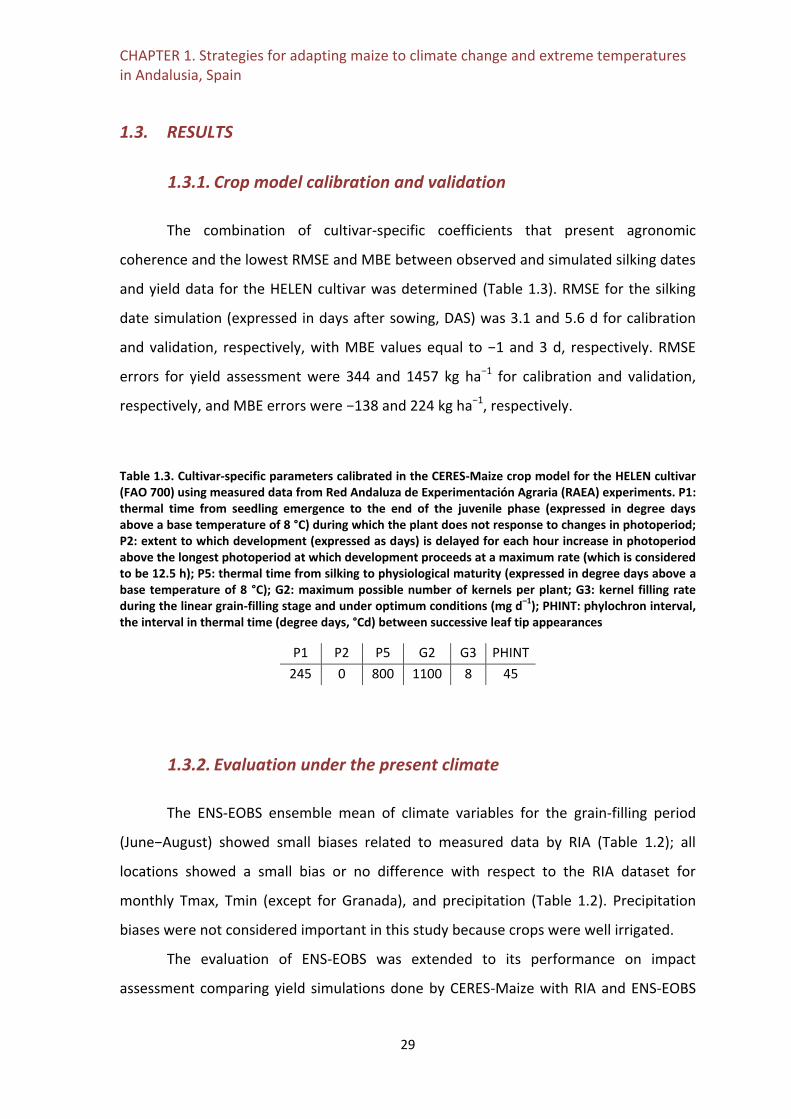
CHAPTER 1. Strategies for adapting maize to climate change and extreme temperatures in Andalusia, Spain
29
1.3. RESULTS
1.3.1. Crop model calibration and validation
The combination of cultivar-specific coefficients that present agronomic
coherence and the lowest RMSE and MBE between observed and simulated silking dates
and yield data for the HELEN cultivar was determined (Table 1.3). RMSE for the silking
date simulation (expressed in days after sowing, DAS) was 3.1 and 5.6 d for calibration
and validation, respectively, with MBE values equal to −1 and 3 d, respectively. RMSE
errors for yield assessment were 344 and 1457 kg ha−1 for calibration and validation,
respectively, and MBE errors were −138 and 224 kg ha−1, respectively.
Table 1.3. Cultivar-specific parameters calibrated in the CERES-Maize crop model for the HELEN cultivar (FAO 700) using measured data from Red Andaluza de Experimentación Agraria (RAEA) experiments. P1: thermal time from seedling emergence to the end of the juvenile phase (expressed in degree days above a base temperature of 8 °C) during which the plant does not response to changes in photoperiod; P2: extent to which development (expressed as days) is delayed for each hour increase in photoperiod above the longest photoperiod at which development proceeds at a maximum rate (which is considered to be 12.5 h); P5: thermal time from silking to physiological maturity (expressed in degree days above a base temperature of 8 °C); G2: maximum possible number of kernels per plant; G3: kernel filling rate during the linear grain-filling stage and under optimum conditions (mg d–1); PHINT: phylochron interval, the interval in thermal time (degree days, °Cd) between successive leaf tip appearances
P1 P2 P5 G2 G3 PHINT
245 0 800 1100 8 45
1.3.2. Evaluation under the present climate
The ENS-EOBS ensemble mean of climate variables for the grain-filling period
(June−August) showed small biases related to measured data by RIA (Table 1.2); all
locations showed a small bias or no difference with respect to the RIA dataset for
monthly Tmax, Tmin (except for Granada), and precipitation (Table 1.2). Precipitation
biases were not considered important in this study because crops were well irrigated.
The evaluation of ENS-EOBS was extended to its performance on impact
assessment comparing yield simulations done by CERES-Maize with RIA and ENS-EOBS

CHAPTER 1. Strategies for adapting maize to climate change and extreme temperatures in Andalusia, Spain
30
climate datasets for the baseline period (Table 1.4). The yield difference ranged from
−6.1 % (for Granada) to 0.6 % (for Palma del Rio; Table 1.4). Both simulated time series
showed similar interannual variability (coefficient of variation, CVtime), with the greatest
difference in Granada (Table 1.4).
Table 1.4. Simulated yield run with observed Agroclimatic Information Network of Andalusia (RIA) data (2001–2010), and interannual variability (coefficient of variation, CVtime). Difference (% of yield) regarding RIA-derived simulations and those conducted with the bias-corrected ensemble ENS-EOBS for the baseline period (1981–2010), and CVtime for these simulations
Climate data used in the crop simulations
Location
RIA ENS-EOBS (%) vs RIA
Yield
(kg ha-1) CVtime
Yield difference
(%) CVtime
Alcalá del Río 16177 8.7 % 1.9 7.3 %
Lora del Río 16055 10.8 % 1.1 7.7 %
Palma del
Río 16094 10.8 % 0.6 7.4 %
Córdoba 15961 7.5 % 1.0 7.7 %
Granada 16966 4.5 % -6.1 8.6 %
1.3.3. Impact and adaptation projections
Simulated phenological dates for Palma del Río (representative of Guadalquivir
locations) and Granada are shown in Fig. 1.2 for B, NF, and FF periods. As GDD
accumulated faster in future climate, both silking (anthesis date, ADAT) and maturity
(MDAT) dates occurred earlier compared to the baseline simulations when sowing date
was not changed, leading to a shorter grain-filling duration (MDAT − ADAT), especially in
the FF period (ca. 17 d for the Guadalquivir locations and 20 d for Granada).
The simulated yield impact for irrigated maize, considering an optimal irrigation
schedule for the ENS-EOBS ensemble mean, is shown in Table 1.5 for the B, NF, and FF
periods and for the 5 locations. The results show a decrease in maize yield, greater in FF,
when yield decrease was ca. 6−7 % at Guadalquivir locations and ca. 20 % in Granada.
However, these effects when compared to the B period were only statistically significant
in Córdoba and Granada (Table 1.5).

CHAPTER 1. Strategies for adapting maize to climate change and extreme temperatures in Andalusia, Spain
31
Interannual variability (CVtime in % for the 30 yr period) in the future (NF and FF)
was ca. 8 % for all Guadalquivir locations, similar to that of the baseline simulations
(Table 1.5). Granada showed a higher increase in variability, especially in the FF (ca. 15
%). The spread or uncertainty related to the differences among the 12 RCM projections
that form ENS-EOBS was measured by the coefficient of variation among them
(CVensemble, %). This spread was similar for all locations (CVensemble: 7−8 %), decreasing
slightly in the FF, except for Granada, where it increased up to ca. 12 % (Table 1.5).
These results show that recovering the baseline yields, particularly in Granada,
requires adaptation measures. The first adaptation proposed consisted of earlier sowing
dates (Fig. 1.3a,b).
Figure 1.2. Simulated phenology for the baseline period (1981−2010), near future (2021−2050), and far future (2071−2100): (a) anthesis date (ADAT), (b) maturity date (MDAT), and (c) grain-filling duration (MDAT − ADAT). DOY: day of the year
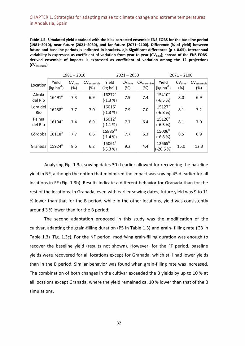
CHAPTER 1. Strategies for adapting maize to climate change and extreme temperatures in Andalusia, Spain
32
Table 1.5. Simulated yield obtained with the bias-corrected ensemble ENS-EOBS for the baseline period (1981–2010), near future (2021–2050), and far future (2071–2100). Difference (% of yield) between future and baseline periods is indicated in brackets. a,b Significant differences (p < 0.05). Interannual variability is expressed as coefficient of variation from year to year (CVtime); spread of the ENS-EOBS-derived ensemble of impacts is expressed as coefficient of variation among the 12 projections (CVensemble)
1981 – 2010 2021 – 2050 2071 – 2100
Location Yield
(kg ha-1) CVtime
(%) CVensemble
(%) Yield
(kg ha-1) CVtime
(%) CVensemble
(%) Yield
(kg ha-1) CVtime
(%) CVensemble
(%)
Alcalá del Río
16491a 7.3 6.9 16272a (-1.3 %)
7.9 7.4 15410a (-6.5 %)
8.0 6.9
Lora del Río
16238a 7.7 7.0 16016a
(-1.3 %) 7.9 7.0
15127a (-6.8 %)
8.1 7.2
Palma del Río
16194a 7.4 6.9 16012a
(-1.1 %) 7.7 6.4
15126a (-6.5 %)
8.1 7.0
Córdoba 16118a 7.7 6.6 15885ab
(-1.4 %) 7.7 6.3
15006b (-6.8 %)
8.5 6.9
Granada 15924a 8.6 6.2 15061a
(-5.3 %) 9.2 4.4
12665b (-20.6 %)
15.0 12.3
Analyzing Fig. 1.3a, sowing dates 30 d earlier allowed for recovering the baseline
yield in NF, although the option that minimized the impact was sowing 45 d earlier for all
locations in FF (Fig. 1.3b). Results indicate a different behavior for Granada than for the
rest of the locations. In Granada, even with earlier sowing dates, future yield was 9 to 11
% lower than that for the B period, while in the other locations, yield was consistently
around 3 % lower than for the B period.
The second adaptation proposed in this study was the modification of the
cultivar, adapting the grain-filling duration (P5 in Table 1.3) and grain- filling rate (G3 in
Table 1.3) (Fig. 1.3c). For the NF period, modifying grain-filling duration was enough to
recover the baseline yield (results not shown). However, for the FF period, baseline
yields were recovered for all locations except for Granada, which still had lower yields
than in the B period. Similar behavior was found when grain-filling rate was increased.
The combination of both changes in the cultivar exceeded the B yields by up to 10 % at
all locations except Granada, where the yield remained ca. 10 % lower than that of the B
simulations.

CHAPTER 1. Strategies for adapting maize to climate change and extreme temperatures in Andalusia, Spain
33
Figure 1.3. Projections of crop yield, impacts, and adaptations for the 12 regional climate model (RCM) projections of the bias-corrected ensemble ENS-EOBS at each location. The y-axis shows the simulated yield; x-axis specifies the simulation: yield for 1981−2010 (baseline), yield without adaptation for 2051−2071 or near future (NF), for 2071−2100 or far future (FF), and adaptations for NF (NF; adaptation) and FF (FF; adaptation). Adaptations are as follows: (a) sowing date advanced 15, 30, 45, and 60 d in the NF; (b) sowing date advanced 15, 30, 45, and 60 d in the FF; (c) increase in the CERES cultivar coefficients for duration of grain-filling (P5) and grain-filling rate (G3), and increase in both P5 and G3, in the FF; (d) combination of sowing 30 d earlier and increased P5, sowing 30 d earlier and increased G3, and sowing 30 d earlier and increased P5 and G3, in the FF. Boxplots show the distribution of the 12 RCM-derived results: box: 2nd and 3rd quartiles; line in the middle: median; point in the middle: mean; whiskers: maximum and minimum

CHAPTER 1. Strategies for adapting maize to climate change and extreme temperatures in Andalusia, Spain
34
The advance in sowing dates and the changes in crop phenology were combined
in several ways, to improve Granada’s result, and to explore the potential of these
combinations for the Guadalquivir locations (Fig. 1.3d for FF). When the sowing date was
advanced by 30 d and the cultivar-specific coefficients were set to P5 = 850 GDD and G3
= 9 mg d−1, the B yields were recovered at Granada (0.2 % of change). The same
phenology, but with a sowing date 45 d earlier, showed an even higher yield for Granada
(4.5 % of change). However, the 30 d option was the adaptation selected (hereafter
called ADPS), valid for all locations to minimize disruption of the current cropping
system, as large shifts in sowing dates may imply changes in crop rotations.
An average reduction of ETc of 10 and 25 % was found for the NF and FF,
respectively (Table 1.6). The baseline ETc values were lower for Granada than for the
Guadalquivir locations. IRR ranged from 668 mm for Granada to 726 mm for the
Guadalquivir Valley. As a consequence of the ETc reductions, IRR showed decreases of
around 9% in all locations for the NF period, which were slightly higher for the
Guadalquivir locations (ca. 25 %) compared to Granada (ca. 16%) by the end of the 21st
century. These reductions in ETc and IRR values were accompanied by an increase in
water productivity (Table 1.6); both TWP and IWP were higher for all locations in NF and
FF compared with baseline values.
In the ADPS simulations for Guadalquivir locations, ETc values increased around
3.5 % compared with the results obtained without adaptation strategies. This increase
was around 9.5 % for Granada. The IRR results showed limited changes for the
Guadalquivir locations (0.4 and −1.1 %) and an increase for Granada (7 and 6 %) for NF
and FF periods, respectively, compared with the same period

CHAPTER 1. Strategies for adapting maize to climate change and extreme temperatures in Andalusia, Spain
35
Table 1.6 Mean values of crop cycle duration, maturity date (MDAT), total season evapotranspiration (ETc), total irrigation requirements (IRR), water productivity (TWP), and irrigation water productivity (IWP), with the 12 regional climate models of the bias-corrected ensemble ENS-EOBS, for the baseline period (1981–2010), near future (2021–2050), and far future (2071–2100), with (ADPS) and without ('Impact') adaptation. ADPS: Adaptation selected (sowing date 30 d earlier, P5 = 850 GDD and G3 = 9 mg d−1),), DOY: day of the year
Location Result 1981–2010 2021–2050 2071–2100
Baseline Impact ADPS Impact ADPS
Alcala del Río
Crop cycle (d) 138 132 154 121 143
MDAT (DOY) 200 194 187 183 175
ETC (mm) 722 650 673 543 555
IRR (mm) 729 659 658 554 543
TWP (kg m–3) 3.1 3.5 4.2 4.1 4.9
IWP (kg m–3) 2.3 2.5 3.1 2.8 3.5
Lora del Río
Crop cycle (d) 137 131 153 120 141
MDAT (DOY) 202 196 189 185 177
ETC (mm) 705 635 665 532 550
IRR (mm) 699 631 633 531 527
TWP (kg m–3) 3.1 3.5 4.1 4.0 4.8
IWP (kg m–3) 2.3 2.6 3.1 2.9 3.5
Palma del Río
Crop cycle (d) 137 130 154 121 143
MDAT (DOY) 203 196 190 186 179
ETC (mm) 730 658 682 555 566
IRR (mm) 768 697 697 592 580
TWP (kg m–3) 3.1 3.5 4.2 4.0 4.9
IWP (kg m–3) 2.1 2.3 2.9 2.6 3.2
Córdoba
Crop cycle (d) 138 131 154 121 143
MDAT (DOY) 204 197 191 187 180
ETC (mm) 713 643 673 539 562
IRR (mm) 710 645 653 542 544
TWP (kg m–3) 3.1 3.5 4.1 4.0 4.8
IWP (kg m–3) 2.3 2.5 3.0 2.8 3.4
Granada
Crop cycle (d) 126 119 142 108 129
MDAT (DOY) 225 217 211 205 198
ETC (mm) 688 623 684 525 575
IRR (mm) 668 608 649 527 560
TWP (kg m–3) 3.2 3.4 3.9 3.4 4.1
IWP (kg m–3) 2.4 2.5 2.8 2.5 2.9

CHAPTER 1. Strategies for adapting maize to climate change and extreme temperatures in Andalusia, Spain
36
1.3.4. Extreme events
The fHS parameter increased for all locations and for both NF and FF periods (Fig.
1.4). The increase for the future periods compared with the B period was lower in the
Guadalquivir Valley locations than for Granada. The implementation of ADPS in NF
resulted in a slight decrease of fHS in the Guadalquivir locations, and in a minor increase
in FF. In Granada, the compensation was lower, increasing in both NF and FF compared
with the B period.
Figure 1.4 Heat stress index (fHS) for the baseline period (1981–2010), for the near future (2021–2050) without adaptation ('impact') and with the adaptation selected (ADPS, sowing date 30 d earlier, P5 = 850 GDD and G3 = 9 mg d−1), and for the far future (2071–2100) without adaptation ('impact') and with the ADPS, for all locations (top to bottom: Alcalá del Río, Lora del Río, Palma del Río, Córdoba, Granada). Lower part of the box: first quartile; line in the middle: second quartile or median; upper part of the box: third quartile; point in the middle: mean; vertical lines (whiskers): maximum and minimum
The fdmgn parameter showed an increase in all locations for the future periods
(Fig. 1.5), as expected due to the fHS results. This increase was more evident in Granada
than in the Guadalquivir locations at the end of the 21st century. This index was also
evaluated with the ADPS adaptation for the future periods, compared with the B period
without ADPS (Fig. 1.5), showing a decrease in production damage for NF at the
Guadalquivir locations equal to 26 %, and a slight increase in Granada (5 %). This trend

CHAPTER 1. Strategies for adapting maize to climate change and extreme temperatures in Andalusia, Spain
37
continued into the FF, with a decrease in production damage in the Guadalquivir
locations of 8 % and an increase in Granada (8 %) compared to B.
The uncertainty of the fdmgn projections was evaluated in terms of the ensemble
spread: Granada showed the highest ensemble spread for the FF period, with
differences between maximum and minimum fdmgn values of 0.7, compared with 0.4 for
the Guadalquivir locations. Equally, FF was the period with higher spread among the
projections when adaptation was simulated, for all locations (Fig. 1.5).
Figure 1.5. Same as for Fig. 1.4, but for normalized production damage index (fdmgn)
1.4. DISCUSSION
1.4.1. Impacts
The model parameterization and the errors of model calibration and validation
were similar to those determined in previous studies (Meza et al., 2008; Vučetić 2011;
Angulo et al., 2013; Moradi et al., 2013).
Granada presented different results than the other locations. Granada station is
not well represented by the E-OBS grid cell. The complex orography of the Granada area
has a lower altitude (633 m), compared to the mean grid altitude of 1034 m for both E-
OBS and ENS-EOBS. This could explain the higher bias in temperatures, which was not
CHAPTER 1. Strategies for adapting maize to climate change and extreme temperatures in Andalusia, Spain
38
improved by bias correction. Also, this could explain why yield simulation could not be
improved and why there was high uncertainty of crop projections at Granada.
In the Guadalquivir locations, yield decrease in the FF period was moderate and
smaller than indicated by previous projections for the Guadalquivir basin (Guereña et al.,
2001; Garrido et al., 2011; Rey et al., 2011). However, yield impacts in Granada were in
agreement with those previous studies. This response at Granada could be explained
because the grain-filling duration projected for the FF period decreased more than at
the other locations.
The overall uncertainty of these projections is low compared to other studies
(Ruiz-Ramos and Mínguez, 2010). This is a consequence of (1) conducting simulations
under an optimum irrigation supply, excluding uncertainty linked to precipitation, which
is usually high for the IP (Sánchez and Miguez-Macho, 2010); and (2) the use of the bias-
corrected ensemble ENS-OBS. Furthermore, the variability of climate conditions in the
selected locations adds value to the study and increases the representativeness of the
result.
1.4.2. Agronomic adaptations
Earlier sowing dates showed positive effects in agreement with previous studies
(Tubiello et al., 2000; Moriondo et al., 2011). In Andalusia, the optimum sowing date is
determined by matching the crop cycle to a period of temperatures warm enough to not
limit maize growth, but cool enough to allow for a long crop cycle, and especially a long
grain-filling period. Our results are relevant for adaptation studies, which usually use
static sowing dates through the adaptation simulation for simplicity (e.g. Moriondo et
al., 2011). A simple rule for computing the sowing date as a function of the year or
decade could be more realistic and easy to implement.
Ideotypes taking advantage of the changed conditions with a longer and more
efficient grain-filling period would be feasible, and breeders are currently investigating
increasing leaf area duration (LAD), stay-green trait (Chen et al., 2013; Ning et al., 2013),
and extending the duration of grain-filling (Tollenaar and Lee, 2011). The 2 coefficients
affecting the targeted variables were modified within a feasible range, taking as
reference their values from previously calibrated cultivars. The simulations confirmed

CHAPTER 1. Strategies for adapting maize to climate change and extreme temperatures in Andalusia, Spain
39
that these changes are promising, although in Granada, further adaptations would be
needed.
The combination of both strategies confirms that their effects are not additive.
The objective of recovering the potential baseline yield in Granada was accomplished
with the combined adaptation ADPS. Future farming will exhibit a yield gap (Cassman et
al., 2003; van Ittersum et al., 2013) compared to our simulations. The crop model does
not simulate some processes, such as pests and diseases that could be enhanced by
longer crop cycles, together with elevated temperatures. Also, the current model
description of some processes might not be robust enough under future conditions
(Prasad et al., 2006). Therefore, the actual yields should be lower than our projections
(ca. 36 %; see MAGRAMA 2013 for current yields).
For crop irrigation requirements (IRR), Mínguez et al., (2005) determined
increases in crop water requirements; however, Yano et al., (2007) reported an IRR
reduction of 25 % in 2079 for Turkey, and Guereña et al., (2001) showed a reduction of
16 % for maize in Spain in 2050, due to the CO2 concentration increase. In our study, the
observed decrease in estimated IRR for future periods without adaptation strategies
agrees with these studies, and could be explained by: (1) reduction of the crop cycle
duration due to warmer temperatures, avoiding the crop cycle going into the summer;
and (2) the ETc reduction due to decreased stomatal conductance as an effect of future
CO2 concentrations (Cure and Acock, 1986; Ainsworth and Long, 2005).
IRR values under the ADPS simulations were lower for the NF and FF periods than
for the B period. This reduction could be due to the earlier maturity dates, avoiding the
driest and hottest period for the maize crop.
The increased water productivity (TWP) in the future periods could be related to
reduced stomatal conductance (Leakey et al., 2006; Vanuytrecht et al., 2012). When the
adaptations were implemented, TWP and IWP increased because yield increased more
than crop transpiration and irrigation water requirements, respectively.

CHAPTER 1. Strategies for adapting maize to climate change and extreme temperatures in Andalusia, Spain
40
1.4.3. Extreme Tmax events
In this study, we considered daily Tmax instead day-time Tday: (1) to take into
account that cultivars used in the Mediterranean region could have more heat tolerance
than those of colder latitudes; and (2) to test another possible adaptation consisting of
developing cultivars with further tolerance to high temperatures.
The increase in projected heat stress index resulted in an increase in production
damages at the end of the 21st century, in agreement with previous results (Beniston et
al., 2007, Ruiz-Ramos et al., 2011). The adaptation strategies tested here, such as the
crop cycle change and the consideration of new cultivars, diminish negative impacts at
field, regional, and European levels (Olesen et al., 2011). However, our results
emphasize that the adaptations for these events must be local, due to differences in the
spatial pattern of extreme events (Teixeira et al., 2013).
1.5. CONCLUSIONS
The CERES-Maize crop model was calibrated and validated using experimental
data for 5 semi-arid locations, spanning an overall time period of 9 yr, obtaining a locally
tailored approach for yield and irrigation needs estimation. Analysis of how extreme
events can enhance or reduce the impacts, and the effect of adaptation strategies, is
essential. The methodological improvement obtained with bias correction increased the
quality of the climate data inputs.
A negative impact of climate change on irrigated maize yield was simulated due
to (1) the shorter crop cycle, and (2) an increase in the frequency of events generating
heat stress. The implementation of adaptation strategies consisting of a combination of
earlier sowing dates and cultivars with a more efficient grain-filling period could
compensate both effects, and even increase the maize yield in southern Spain. In
parallel, irrigation requirements were reduced around 25 % for future periods compared
with the baseline period, both with and without adaptation strategies, due to the
reduction in ETc and higher water use efficiency.

CHAPTER 1. Strategies for adapting maize to climate change and extreme temperatures in Andalusia, Spain
41
Acknowledgements
This work was financially supported by FACCE MACSUR − Modelling European
Agriculture with Climate Change for Food Security, a FACCE JPI knowledge hub, by
Consejería de Innovación, Ciencia y Empresa Junta de Andalucía (AGR-6126 project), and
by MULCLIVAR, from the Spanish Ministerio de Economía y Competitividad (MINECO,
CGL2012-38923-C02-02). We are grateful to Alfredo Sanchez for technical support.

42

43
CHAPTER 2. MODELLING THE IMPACT OF
HEAT STRESS ON MAIZE YIELD FORMATION
This Chapter is the result of a stay at University of Bonn from 01/02/2015 to 30/03/2015, being Dr. Thomas Gaiser the supervisor of the stay. Submitted: Gabaldón-Leal, C., Webber, H., Otegui, M., Slafer, G., Gaiser, T., Lorite, I.,
Ruiz-Ramos, M., and Ewert, F. (Submitted 8 April 2016. Field Crops Research Journal.
Under review)

44

CHAPTER 2. Modelling the impact of heat stress on maize yield formation
45
ABSTRACT
The frequency and intensity of extreme high temperature events is expected to increase
with climate change. Higher temperatures near anthesis have a large and negative effect
on maize (Zea mays, L.) grain yield. While crop growth models are commonly used to
assess climate change impacts on maize and other crops, it is only recently that they
have accounted for such heat stress effects, despite limited field data availability for
model evaluation. There is also increasing awareness but limited testing about the
importance of canopy temperature as compared to air temperature for heat stress
impact simulations. In this study, four independent irrigated field trials with controlled
heating imposed with polyethylene tents were used to develop and evaluate a heat
stress response function in the crop modeling framework SIMPLACE, in which the Lintul5
crop model was combined with a canopy temperature model. A dataset from Argentina
with the temperate hybrid Nidera AX 842 MG (RM 119) were used to develop a yield
reduction function based on accumulated hourly stress thermal time above a critical
temperature of 34 °C. A second dataset from Spain with a FAO-700 cultivar was used to
evaluate the model with daily climate inputs in two sets of simulations. The first was
used to calibrate SIMPLACE for conditions with no heat stress, and the second was used
to evaluate SIMPLACE under conditions of heat stress using the reduction factor
obtained with the Argentine dataset. Both sets of simulations were conducted twice; the
heat stress function was alternatively driven with air and simulated canopy temperature.
Grain yield simulated under heat stress conditions improved when using canopy
temperature instead of air temperature (RMSE equal to 175 and 309 g m-2, respectively).
For the irrigated and high radiative conditions, raising the critical threshold temperature
for heat stress to 39 °C improved yield simulation using air temperature (RMSE: 221 g m-
2) without the need to simulate canopy temperature (RMSE: 175 g m-2). However, this
approach of adjusting thresholds is only likely to work in environments where climatic
variables and the level of soil water deficit are constant, such as irrigated conditions and
are not appropriate for rainfed production conditions.
KEYWORDS: Heat stress; Maize; Zea mays (L); Crop models.

CHAPTER 2. Modelling the impact of heat stress on maize yield formation
46
2.1. INTRODUCTION
The frequency of extreme temperature (Alexander et al., 2006; IPCC, 2007; Orlowsky
and Seneviratne, 2012) and drought (Alexander et al., 2006) events has increased across
many world regions in the past 60 years, and is expected to further increase (Beniston et
al., 2007; Seneviratne et al., 2012). Together with higher mean temperatures, these
extreme events are expected to cause negative impacts on crop growth (Seneviratne et
al., 2012; Gourdji et al., 2013). Large-scale observational studies analyzing maize yield
and temperature records indicate that large yield losses are associated with even brief
periods of high temperatures when crop-specific high temperature thresholds are
surpassed. French maize yields over the past 50-years were found to have decreased as
the number of days with maximum air temperature above 32 °C increased (Hawkins et
al., 2013). Likewise, a panel analysis of maize yields in the US, determined that yield
decreased with cumulative degree days above 29 °C (Schlenker and Roberts, 2009).
Similarly, Lobell et al. (2011) detected maize yield losses across Sub-Saharan Africa
ranging from 1 to 1.7 % (depending on water availability) per each degree day above 30
°C.
Maize yield is largely determined during a rather narrow window of time of four
to five weeks bracketing silking (Fischer and Palmer, 1984; Otegui and Bonhomme,
1998). It is during this time that crop growth rates strongly determine the number of
grains set (Otegui and Bonhomme, 1998), a key determinant of final grain yield (Fischer
and Palmer, 1984). This is why this period is referred to as “critical” for maize yield
determination with a high sensitivity to abiotic stress (Fischer and Palmer, 1984; Kiniry
and Ritchie, 1985; Grant et al., 1989; Lizaso et al., 2007). The mechanisms of yield
reduction with high temperatures are associated with reductions in both source and sink
capacity. Equally crop development rate, photosynthesis and respiration rates also
respond non-linearly to high temperatures (Lobell et al., 2011), but the reducing effects
on these processes are reversed when temperatures return to optimal ranges (Rattalino
Edreira and Otegui, 2012; Ordóñez et al., 2015). Nevertheless, reductions in net
assimilation (photosynthesis plus respiration) that produce a marked decrease in plant
growth rate can result in large yield reductions if they occur during the critical period for
kernel number determination (Andrade et al., 1999, 2002). The reduction in sink

CHAPTER 2. Modelling the impact of heat stress on maize yield formation
47
capacity can be caused by direct high temperature effects on flowering dynamics, ovary
fertilization or grain abortion, with resulting losses in grain number being irreversible
(Herrero and Johnson, 1980; Rattalino Edreira et al., 2011; Ordóñez et al., 2015).
Evidence from field trials has demonstrated that when heating was performed
during the critical period, reductions in maize yield were very large (Cicchino et al., 2010;
Rattalino Edreira and Otegui, 2012; Ordóñez et al., 2015). These reductions were
independent of the negative effects of heat on pollen viability (Rattalino Edreira et al.,
2011; Ordóñez et al., 2015), and were predominantly driven by reduced ovary
fertilization of pollinated spikelets exposed to temperatures above 35 °C (Dupuis and
Dumas, 1990). The reduction in grain number due to kernel abortion was the main effect
of high temperatures during flowering in other work (Rattalino Edreira and Otegui, 2013;
Ordóñez et al., 2015).
Various studies have identified a threshold optimum temperature of about 30
(Gilmore and Rogers, 1958; Tollenaar et al., 1979) to 35 °C (Jones and Kiniry, 1986) for
maize. In field trials with controlled heating, Cicchino et al. (2010b) determined the
critical optimum temperature at flowering in two years as 35.5 ± 1.3 °C and 32.2 ± 1.1 °C
with a temperate hybrid. Porter and Semenov (2005) reported that temperatures above
36 °C reduced pollen viability in this species. Finally, Sánchez et al. (2014) reported 37.3
and 36 °C for the flowering and grain filling period, respectively, as the threshold
optimum temperature.
Some evidence suggests that the crop canopy temperature better explains yield
reductions associated with surpassing high temperature thresholds better than air
temperature (Craufurd et al., 2013; Siebert et al., 2014; Webber et al., 2016). The
differences between air temperature and the temperature of the canopy surface can
differ significantly depending on the irrigation conditions, as the irrigation have a cooling
effect on the ambient that could reduce the canopy temperatures (Lobell et al., 2008) by
as much as 10° C (Kimball et al., 2015) . However under rainfed conditions when soil
water is limiting, or when transpiration rates are low due to low vapor pressure deficit,
crop canopy temperature can increase above air temperature leading to yield loss from
high crop temperatures (Lobell et al., 2015). The difference between air and crop canopy
temperature is thought to be critical for heat stress responses as the difference of 1 - 2
CHAPTER 2. Modelling the impact of heat stress on maize yield formation
48
°C can lead to large over or underestimation of yield loss from heat stress (Webber et
al., 2016). While temperature gradients exist within the vertical plant profile (Rattalino
Edreira et al., 2012), it may be sufficient to capture the difference between the canopy
surface and air temperature for simulations at the field and larger scales.
Currently, only a few published crop models include the effects of heat stress on
maize yield and its physiological determinants, such as GLAM (Challinor et al., 2005,
2004), Aquacrop (Raes et al., 2009; Steduto et al., 2012), a modified Cropsyst (Moriondo
et al., 2011) or APSIM maize (Lobell et al., 2015). Additionally, other research groups are
currently developing heat stress modules specific for maize such as Lizaso et al. (2016).
However, no published studies have evaluated model performance under heat stress
using field trials with controlled heating. Consequently, heat stress model development
and testing has been limited by a lack of data from field experiments with the
application of high temperatures compared to a non-heated control. This applies even
more so for modelling the effect of canopy temperature as compared to air
temperature. Without such data, correct attribution of heat stress is difficult to
distinguish from other growth limiting factors.
This study makes use of two independent datasets collected at Argentina and
Spain in which controlled heating was applied to field grown maize crops. These datasets
are used to parametrize and evaluate the performance of a canopy heat stress approach
to account for the negative effects of extreme high temperatures on maize grain yield.
The model performance is evaluated using both air and simulated canopy temperature
as inputs to the heat stress module. These functions are included in crop models to be
applied at field and larger scales.

CHAPTER 2. Modelling the impact of heat stress on maize yield formation
49
2.2. MATERIAL AND METHODS
2.2.1. Experimental data
2.2.1.1. Argentine experiments
To develop a relationship with high temperatures, two experimental datasets
obtained at Pergamino (33°56´ S, 60°34´ W), Argentina, were used. Crops were
cultivated under field conditions, but with controlled heat stress. These two experiments
were carried out during two growing seasons (Table 2.1), in 2006/2007 (A1) and
2007/2008 (A2). Details of crop husbandry can be found in Cicchino et al. (2010a,
2010b). Briefly, the cultivar used was the temperate hybrid Nidera AX 842 MG, classified
as 119 for relative maturity (Peterson et al., 1973). The experiments were fully fertilized
and irrigation was supplied to avoid water stress. Crop management ensured minimal
weed, pest and disease pressure. Two temperature regimes were applied (C: control
plots; H: heated plots). The timing of heating was applied was an experimental
treatment with two levels: GS1 heating between the appearance of the 11th leaf (V11 of
Ritchie and Hanway, 1982) and tasseling and GS2 with heating from tasseling to 15days
after silking . In A1, only GS1 has applied, whereas in A2, heating was applied for each of
GS1 and GS2. The duration of heating periods in GS1 and GS2 (ca. 15-20 days) was based
on dates of VT and silking of control plots. Shoot biomass was estimated based on plants
tagged before heating. Yield (Y) and yield components (kernel number per plant and
individual kernel weight) were determined by harvesting ears with grains of each tagged
plant, oven dried until constant weight and then weighed.
Temperature regime treatments were obtained by placing polyethylene shelters
over two consecutive central rows of plots to increase the temperature via the
greenhouse effect created by the shelters. In the heated treatments (H), the shelters
reached close to the ground surface, except for one side that remained open to
approximately 15 cm above ground level. For the control treatments (C), the South
facing side remained open up to 1.4 m above the soil surface. The purpose of the open
shelters in the C treatment was to avoid differences in solar radiation between
treatments. Hourly records of air temperature in C and H plots were obtained by means

CHAPTER 2. Modelling the impact of heat stress on maize yield formation
50
of sensors (TC1047, Microchip Technologies, Chandler, AZ) installed at ear height and
connected to dataloggers (Temp-Logger, Cavadevices, Buenos Aires, Argentina). Solar
radiation, wind speed and relative humidity data were collected from a weather station
500 m from the experimental site. The Argentine experiments were used for
determination of the heat stress reduction factor, but not used for simulations with the
canopy heat stress model, as only the air temperature at ear level (Tair_ear) was recorded
in these experiments.
2.2.1.2. Spanish experiments
Datasets from two field experiments with controlled heating were used in the
model evaluation. These two experiments were arranged into two studies, S1 and S2,
each replicated for two consecutive growing seasons. The first year (2009) was
conducted in Menarguens (41°43’48’’N, 0°44’24’’E) and the following three years (2010,
2011, 2012) in Algerri (41°48’36’’N,0°38’24’’E), both in Lleida, Spain (Table 2.1). Study S1
was carried out in 2009 (S1.1) and 2010 (S1.2) and S2 in 2011 (S2.1) and 2012 (S2.2). The
cultivar Pioneer 31N28 (FAO-700) was used in S1.1, S1.2 and S2.1. For S2.2, Pioneer
33Y72 (FAO700) was used. PR33Y72 is similar to PR31N28 in all traits considered.
Biomass was estimated by above-ground dry weight through oven drying the samples
collected in each plot at maturity. Yield and its components were measured on these
same samples. Additional details are reported in Ordoñez et al. (2015). Similar to the
Argentine experiments, crop management ensured that there was minimal water,
nitrogen or biotic stresses during the cropping season. The temperature regimes for S1
were (i) C: a control with no imposed heating, (ii) S1_Pre: heating imposed from 15 days
before silking (Silk-15d) to maturity, and (iii) S1_Post: heating imposed from 15 days
after silking (Silk+15d) to maturity. Heating periods were about 76 days in S1. The
temperature regimes for S2 were (i) C, as described above, (ii) S2_Pre: heating imposed
from 7 days before silking (Silk-7d) to 9 days after silking (Silk+9d), and (iii) S2_Post:
heating imposed from 14 days after silking (Silk+14d) to 32 days after silking (Silk+32d).
Heated treatments were established by means of polyethylene shelters mounted on
structures of 3–3.5 m height (leaving the bottom 0.3 m open). As in the experiments
from Agentina, elevated temperatures were obtained due to the greenhouse effect of

CHAPTER 2. Modelling the impact of heat stress on maize yield formation
51
the shelters. Air temperature inside the shelters was measured at tassel (Tair_tas) and ear
levels (Tair_ear).
Tabla 2.1 Details of experiments used in the study
Location Experiment Harvest
Year
Heating treatment
code
Heating treatment
period
Air temperature measurement
level
Argentina
A1 2007 A1_GS1a V11 to VT Ear
A2
2008 A2_GS1 V11 to VT Ear
2008 A2_GS2 VT to
Silk+15d Ear
Spain
S1.1 2009
S1_PreS Silk-15d to
Mat Ear and tassel
S1_PostS Silk+15d to
Mat Ear and tassel
S1.2 2010
S1_ PreS Silk-15d to
Mat Ear and tassel
S1_ PostS Silk+15d to
Mat Ear and tassel
S2.1 2011
S2_ PreS Silk-7d to Silk
+9d Ear and tassel
S2_ PostS Silk+14d to
Silk+32 Ear and tassel
S2.2 2012
S2_ PreS Silk-7d to Silk
+9d Ear and tassel
S2_ PostS Silk+14 to Silk+32d
Ear and tassel
a Abbreviations: d, days; GS, Growing stage; Mat, Maturity; PostS, Post silking heating; PreS, Pre silking heating; Silk, Silking; VT, tasseling.
2.2.2. Model description
The maize heat stress model was developed and tested in SIMPLACE (Scientific
Impact assessment and Modeling PLatform for Advanced Crop and Ecosystem
management) modeling framework (Gaiser et al., 2013) together with the Lintul5 model
(Wolf, 2012), the DRUNIR water balance model (Spitters and Schapendonk, 1990; Van
Oijen and Leffelaar, 2008) and the CanopyT model (Webber et al., 2016). The combined
model is SIMPLACE<Lintul5, DRUNIR, CanopyT, HeatStressHourly>, further referred to as
SIMPLACE <Lintul5,HS,Tc>. The Lintul5 model is radiation use efficiency (RUE) based,
that accounts for water and nutrient limitation. Crop development rates are a function
of 24-h mean temperature above a base temperature, variety-specific parameters, and

CHAPTER 2. Modelling the impact of heat stress on maize yield formation
52
photoperiod sensitivity. Two parameters (TSUM1 and TSUM2) account for the thermal
time required from emergence to anthesis and anthesis to maturity, respectively.
Biomass growth is determined as the product of RUE and the amount of
photosynthetically active radiation (PAR) that is intercepted by the crop (PARi). PARi is
determined using Beer’s Law as a function of the leaf area index (LAI). LAI growth is
exponential, early determined by biomass accumulation and a time-varying specific leaf
area (SLA). RUE also varies as a function of the crop development stage, and is reduced
as a function of water stress. Water stress occurs when the crop transpiration is lower
than the rate of potential transpiration. Partitioning of biomass to roots, stems, leaves
and grains varies with the crop development stage, with partitioning to roots increasing
under water stress. Lintul5 also has a RUE correction factor (RTMCO) that reduces RUE
when daily mean temperature rises above 35 °C throughout the entire growing season.
Consideration of canopy temperature (Tcan) allows accounting for the feedback
between crop water status and crop temperature. The CanopyT model calculates hourly
Tcan using daily climate data with an energy balance approach correcting for atmospheric
stability conditions using the Monin-Obukhov Similarity Theory (Webber et al., 2016).
The model makes simplifications about the canopy resistance term to avoid the need to
calculate stomatal conductance. It is assumed that the upper (warm) temperature limit
(Tcan,upper) for particular weather conditions is reached when the crop does not transpire,
as occurs under conditions of high water stress. Likewise, the lower (cool) temperature
limit (Tcan,lower) is reached when the crop is transpiring at its maximum potential rate, as
occurs under non-water limiting conditions. Actual Tcan is determined by interpolating
between these two extremes as a function of crop water stress. This simplification
renders it suitable for application in crop models aimed at field, regional and larger
scales. The evaluated model approach compared very well to other approaches used to
simulate Tcan (Webber et al., 2015).
The heat stress module developed here, HeatStressHourly, is based on an
approach implemented in the APSIM crop model (Lobell et al., 2015), modified for
hourly time steps with the possibility to use either simulated canopy (Tcan) or air
temperature (Tair). Daily minimum and maximum values of Tair are converted to hourly
values using a sinusoidal function as in Goudriaan and van Laar (1994) and Nguyen et al.

CHAPTER 2. Modelling the impact of heat stress on maize yield formation
53
(2014). The module developed here reduces yield (Y) as a function of the hourly stress
thermal time (TThs, in °Ch) (Blumenthal et al., 1991) accumulated above a critical high
temperature threshold (Tcrit) during the critical period for kernel number determination
(between 300 °Cd before and 200 °Cd after silking, ca. 30 days bracketing silking).
2.2.3. Simulation steps
Model development and testing consisted of three main steps: (i) heat stress
yield reduction factor determination, (ii) crop model calibration, and (iii) model
validation (see Fig. 2.1). Broadly speaking, the Argentine experiments were used in Step
1 to establish the yield reduction heat stress factor (RedHS), by comparing the control
and heated treatments. The Spanish dataset was used in Steps 2 and 3, for calibration
(using the experiments without heat stress) and validation of the combined model
SIMPLACE <Lintul5,HS,Tc> with the heat stress experiments, respectively. Simulations
were conducted twice using two different estimates of hourly temperature (Th) to
calculate hourly stress thermal time (TThs) (Eq. 1); first using hourly Th = Tair, and
secondly with hourly Th = Tcan, as input:
𝑇𝑇ℎ𝑠,𝑖 = 𝑇ℎ,𝑖 − 𝑇𝑐𝑟𝑖𝑡 Eq. [1]
Step 1: To determine RedHS based with a specified critical temperature threshold; air
temperature at ear level (Tear) was used, as it can be considered the actual temperature
experienced by the ear. RedHs was calculated as the reduction in Y per TThs, with Tcrit= 34 °C as
obtained by Cicchino et al. (2010b) with the same set of experiments. Y was normalized (Eq. 2)
with the Y obtained in the control treatment at each experiment, considering the Y in the control
as the maximum Y that can be achieved in a particular year and site under the given conditions.
𝑌𝑛,𝑖 =𝑌𝑜𝑖
𝑌𝑚𝑖 Eq. [2]
Where, Yn,i is normalized Y, Yo,i is the observed Y from the heated treatment and
Ym,i is the maximum Y observed in the control experiment, and i representing the
experiment.
With TThs,i and Yni had been calculated, the RedHS was calculated as

CHAPTER 2. Modelling the impact of heat stress on maize yield formation
54
𝑅𝑒𝑑𝐻𝑆 =∑ (
𝛥𝑌n,i𝛥𝑇𝑇ℎ𝑠,𝑖
)𝑁𝑖=1
𝑁 Eq. [3]
Where, ΔYn is the difference between the Yn,i for the control (equal to 1) and Yn,i
for the heated treatment for each experiment, and ΔTThs,i the difference between the
hourly stress thermal time for the control treatment and the heated treatment. The
index i indicates the experiment/treatment combination (e.g. 1= A1_GS1, 2= A2_GS1
and 3= A2_GS2) and N the total number of experiment/treatments combinations.
Step 2: SIMPLACE <Lintul5,HS,Tc> was calibrated for conditions of no heat stress
using the control treatments in the Spanish dataset following the procedure shown in
Fig. 2.1. The first step was to calibrate the phenology routine (anthesis and maturity
dates) with the parameters TSUM1 and TSUM2. Then the biomass data were used to
calibrate RUE, SLA and RGRLAI (maximum relative increase in LAI). In a final step, Y was
used to calibrate FRTDM (fraction of aboveground biomass to be translocated to seeds).
Final Y was first simulated using the same Tcrit for both Tcan and Tair, and later increasing
the Tcrit for Tair based on the difference in temperatures within the maize canopy
(Rattalino Edreira et al., 2012).
Step 3: Validation of calibrated SIMPLACE <Lintul5,HS,Tc> was performed with
the heated treatments from the Spanish datasets, considering the RedHS factor
obtained in Step 1 and the crop parameters calibrated in Step 2.
Steps 1 to 3 were conducted with each Tair and Tcan, and results compared.
Additionally, simulated Tcan for the Spanish experiments were compared with observed
ear temperature values.

CHAPTER 2. Modelling the impact of heat stress on maize yield formation
55
Figure 2.1. Flowchart illustrating heat stress reduction function development and evaluation procedure. The heat stress reduction factor determination (Step 1) is shown on the left, model calibration (Step 2) on the right, and model evaluation (Step 3) in the bottom. The experiment/treatment combinations considered in each step are shown in parentheses of the grey boxes.
To estimate errors in the calibration process, root mean square error (RMSE),
and mean bias error (MBE) were determined as:
𝑅𝑀𝑆𝐸 = √∑ (𝑆𝑖−𝑂𝑖)
2𝑛𝑖=1
𝑛 Eq. [4]
𝑀𝐵𝐸 =∑ (𝑆𝑖−𝑂𝑖)𝑛𝑖=1
𝑛 Eq. [5]
where Si is the simulated value and Oi the observed value, and i representing the
experiment.

CHAPTER 2. Modelling the impact of heat stress on maize yield formation
56
2.3. RESULTS
2.3.1. Step1: Determination of yield reduction heat stress factor
TThs,i calculated with Tear from A1_GS and A2_GS experiments (Table 2.1) and Tcrit
set at 34 °C showed a negative relationship with Y (Table 2.2). The Y reductions resulting
from heating were larger for A2_GS1 than for A1_GS1, with a mean reduction in Y due to
heating of 683 g m-2 (59.3 % reduction in Yn). Y reduction for A2_GS2 was intermediate
between these values. The relative Y loss per unit TThs between the three
experiment/treatment combinations was A1_GS1 > A2_GS2 > A1_GS2. The mean Y
decrease per unit TThs during the critical period, i.e. RedHS, was -0.0025 °Ch-1 (Table 2.2).
Table 2.2. Relationship between hourly stress thermal time (TThs) based on ear temperature and normalized maize grain yield (Yn) for the Argentine experiments with a critical threshold temperature of 34 °C. The reduction heat stress factor (RedHS) represents the relationship between Yn and TThs.
TThs
(°Ch) Y
(g m-2) Yn
RedHS (°Ch-1)
A1_GS1 control 13.6 1015.5 1 -0.0030
heated 186.8 480.3 0.473
A2_GS1 control 194.5 1254 1 -0.0019
heated 540.4 439.7 0.351
A2_GS2 control 17.1 1161.6 1 -0.0025
heated 261.2 461.6 0.397
Mean -0.0025
2.3.2. Step 2. Model calibration
The crop parameters resulting in the lowest values of RMSE and MBE for
simulation of the control treatments with SIMPLACE are presented in Table 2.3. The RUE
parameter value from emergence to anthesis was 2.7 g MJ-1, and then decreased linearly
from 2.7 g MJ-1 to 2.5 g MJ-1 around mid-grain filling, to 1.3 g MJ-1 at maturity. The other
parameters were kept constant throughout the crop cycle.

CHAPTER 2. Modelling the impact of heat stress on maize yield formation
57
Table 2.3. Crop parameters for cultivar FAO-700. TSUM1: thermal time from emergence to anthesis, TSUM2: thermal time from anthesis to maturity, SLA: specific leaf area, RUE: Radiation use efficiency for biomass production, RGRLAI: Maximum Relative increase in LAI and FRTDM: fraction of aboveground biomass to be translocated to seeds.
TSUM1
(°Cd) TSUM2
(°Cd) SLA
(m2 g-1), RUE*
(g MJ-1) RGRLAI
(m2 m-2 d-1) FRTDM
FAO-700 850 1100 0.014 2.7 - 2.5 - 1.3 0.014 0.01
* Different values corresponding to different crop development stages: 2.7 g MJ-1 from emergence to anthesis; 2.7 to 2.5 g MJ-1 from anthesis to mid grain filling; 2.5 g MJ-1 to 1.3 g MJ-1 from mid grain filling to maturity
Phenological dates from the Spanish experiments were well simulated with
SIMPLACE <Lintul5,HS,Tc> using the TSUM1 and TSUM2 parameters (Table 2.4). RMSE
results for the anthesis and maturity date calibration were ca. 5 and 3 days, respectively.
Table 2.4. Performance of SIMPLACE <Lintul5,HS,Tc> to simulate phenological dates showing simulated (sim) and observed (obs) anthesis and maturity in days after sowing (DAS) for each treatment. The root mean square error (RMSE) and mean bias error (MBE) for each cultivar are shown.
Anthesis (DAS) Maturity (DAS)
Cultivar Year Treatment sim obs RMSE MBE sim obs RMSE MBE
FAO
700
2010
C
87 83
4.7 1.0
159 161
2.8 0.00
2011 89 84 159 155
2012 102 98 167 169
2009 S1_PreS 63 71 -- --
2009 S1_PostS 63 70 -- --
2010 S1_ PreS 85 85 -- --
2010 S1_ PostS 87 83 -- --
2011 S2_ PreS 88 85 -- --
2011 S2_ PostS 89 84 -- --
2012 S2_ PreS 100 103 -- --
2012 S2_ PostS 102 98 -- --
After phenology calibration, the relationships between Tair-tas, Tair-ear, and
simulated Tcan were evaluated using S1_PreS, S1_PostS, S2_PreS and S2_PostS
experiments. Simulated Tcan at 14.00h from the Spanish experiments was similar to
observed daily maximum Tair-ear (Fig.2.2a). During periods with heating, which did not

CHAPTER 2. Modelling the impact of heat stress on maize yield formation
58
entirely correspond with the critical period, the mean difference between simulated Tcan
and observed Tair-ear was 0.1 °C. Both Tcan and Tair-ear were lower than air temperature at
tassel height (Fig.2.2b), with a mean difference between Tair-ear and Tair-tas of
approximately 8.8 °C.
Figure 2.2. Comparison of temperatures: a) Correlation between maximum observed air temperature at ear level (obs Tair_ear) and simulated canopy temperature (sim Tcan). b) Correlation between maximum observed daily air temperature at tassel height (obs Tair_tas) and maximum observed temperature at ear level (obs Tair_ear) as well as simulated canopy temperature (sim Tcan).
Simulated hourly Tair-tas for 14:00 h (from daily measured temperature at tassel
height) and simulated Tcan at 14:00h were compared for three different periods: (1) the
entire growing season, (2) the critical period (-300 +200 °Cd around silking), and (3) the
times when temperatures were above 34 °C within the critical period. Mean differences
of around 5 °C were obtained between simulated Tcan and Tair-tas for the heated
treatments (S1_PreS/PostS and S2_PreS/PostS) during the critical period (Table 2.5). This
difference increased to around 5.7 °C when the temperatures exceeded 34 °C (Table
2.5).
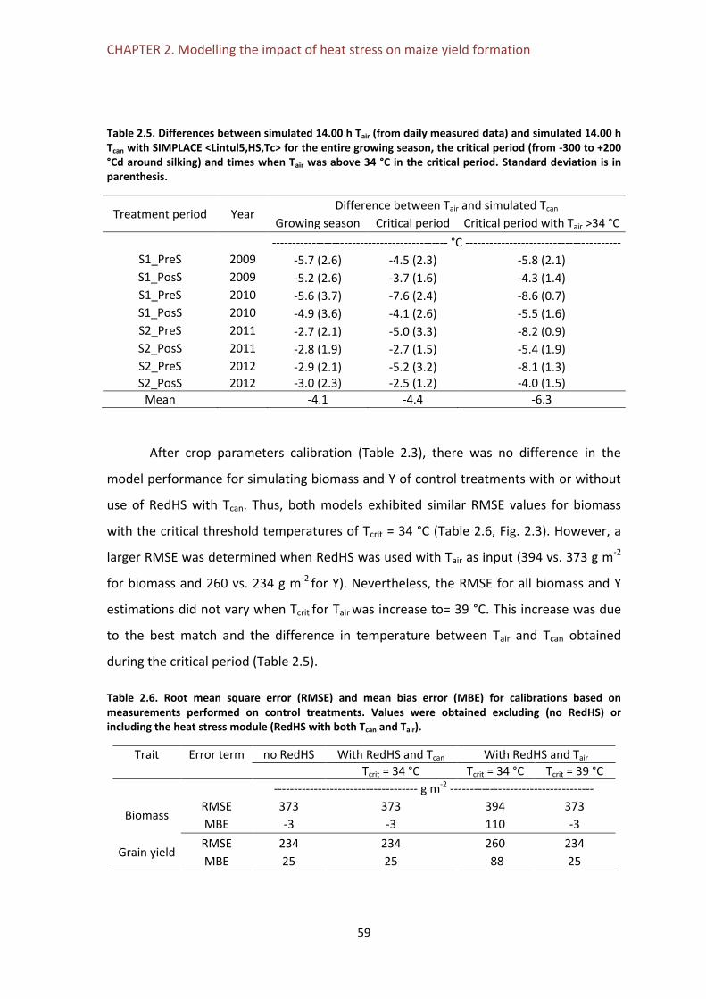
CHAPTER 2. Modelling the impact of heat stress on maize yield formation
59
Table 2.5. Differences between simulated 14.00 h Tair (from daily measured data) and simulated 14.00 h Tcan with SIMPLACE <Lintul5,HS,Tc> for the entire growing season, the critical period (from -300 to +200 °Cd around silking) and times when Tair was above 34 °C in the critical period. Standard deviation is in parenthesis.
Treatment period Year Difference between Tair and simulated Tcan
Growing season Critical period Critical period with Tair >34 °C
-------------------------------------------- °C ---------------------------------------
S1_PreS 2009 -5.7 (2.6) -4.5 (2.3) -5.8 (2.1)
S1_PosS 2009 -5.2 (2.6) -3.7 (1.6) -4.3 (1.4)
S1_PreS 2010 -5.6 (3.7) -7.6 (2.4) -8.6 (0.7)
S1_PosS 2010 -4.9 (3.6) -4.1 (2.6) -5.5 (1.6)
S2_PreS 2011 -2.7 (2.1) -5.0 (3.3) -8.2 (0.9)
S2_PosS 2011 -2.8 (1.9) -2.7 (1.5) -5.4 (1.9)
S2_PreS 2012 -2.9 (2.1) -5.2 (3.2) -8.1 (1.3) S2_PosS 2012 -3.0 (2.3) -2.5 (1.2) -4.0 (1.5)
Mean -4.1 -4.4 -6.3
After crop parameters calibration (Table 2.3), there was no difference in the
model performance for simulating biomass and Y of control treatments with or without
use of RedHS with Tcan. Thus, both models exhibited similar RMSE values for biomass
with the critical threshold temperatures of Tcrit = 34 °C (Table 2.6, Fig. 2.3). However, a
larger RMSE was determined when RedHS was used with Tair as input (394 vs. 373 g m-2
for biomass and 260 vs. 234 g m-2 for Y). Nevertheless, the RMSE for all biomass and Y
estimations did not vary when Tcrit for Tair was increase to= 39 °C. This increase was due
to the best match and the difference in temperature between Tair and Tcan obtained
during the critical period (Table 2.5).
Table 2.6. Root mean square error (RMSE) and mean bias error (MBE) for calibrations based on measurements performed on control treatments. Values were obtained excluding (no RedHS) or including the heat stress module (RedHS with both Tcan and Tair).
Trait Error term no RedHS With RedHS and Tcan With RedHS and Tair
Tcrit = 34 °C Tcrit = 34 °C Tcrit = 39 °C
------------------------------------ g m-2 ------------------------------------
Biomass RMSE 373 373 394 373
MBE -3 -3 110 -3
Grain yield
RMSE 234 234 260 234
MBE 25 25 -88 25

CHAPTER 2. Modelling the impact of heat stress on maize yield formation
60
Figure 2.3. Observed and simulated values of above ground biomass and grain yield (Y) for the control treatments using the model (i) without the heat stress module (no RedHS) (a and b), and (ii) with heat stress module (RedHS) including or Tair (c and d). Upper figures with Tcrit = 34 °C, and lower figures with Tcrit for Tair up to 39 °C and Tcrit for Tcan equal to 34 °C.The line in each figure represents the 1:1 relationship.
2.3.3. Step 3. Model evaluation
The model evaluation with the treatments with heat stress from the Spanish
dataset generated an overestimation of crop biomass when the heat stress module was
not included in the analysis (no RedHS), with greater error for S_PreS than for S_PostS.
This bias was reduced when the heat stress module was added (RMSE declined from 497

CHAPTER 2. Modelling the impact of heat stress on maize yield formation
61
to 416 g m-2). With the inclusion of the heat stress reduction module, biomass in both
treatments (S_PreS and S_PostS) was slightly underestimated. Using the same Tcrit (34
°C) for Tair and Tcan, the error obtained using Tair as an input was higher than using Tcan
(RMSE: 557 vs 395 g m-2); however, when increasing the Tcrit for Tair up to 39 °C the error
was reduced though still slightly greater than that obtained with Tcan using Tcrit= 34 °C
(RMSE: 420 vs 395 g m-2) (Fig. 2.4, Table 2.7).
Figure 2.4 Observed and simulated values of Biomass for pre-silking heating), and post-silking heating using the model (i) without the heat stress module (no RedHS) (a and b) and (ii) with heat stress module (RedHS) including Tcan or Tair (c and d). Upper figures with Tcrit for Tair and Tcan equal to 34 °C, and lower figures with Tcrit for Tair up to 39 °C and Tcrit for Tcan equal to 34 °C. The line in each figure represents the 1:1 relationship.

CHAPTER 2. Modelling the impact of heat stress on maize yield formation
62
Results for Y showed a similar trend to those for biomass, with the highest errors
reported when the model without the RedHS module was used (Table 2.7). Inclusion of
RedHS with Tcan as the input temperature reduced errors for both heated periods
(S_PreS and S_PostS), with a greater improvement in the S_PostS treatment than in the
S_PreS. When Tcrit with Tair was increased to 39 °C, the errors were (i) lower compared to
the model without RedHS, and (ii) slightly higher than using RedHS with Tcan (Fig. 2.5,
Table 2.7).
Figure 2.5. Observed and simulated values of grain yield (Y) with pre-silking heating and post-silking heating using the model (i) without the heat stress module (no RedHS) (a and b) and (ii) with heat stress module (RedHS) including Tcan or Tair (c and d).. Upper figures with Tcrit for Tair and Tcan equal to 34 °C, lower figures with Tcrit for Tair at 39 °C and Tcrit for Tcan equal to 34 °C.

CHAPTER 2. Modelling the impact of heat stress on maize yield formation
63
Table 2.7. Root mean square error (RMSE) of simulated biomass and grain yield for treatments heated during the pre-silking (S_PreS ) or the post-silking (S_PosS) periods, obtained with the model excluding (no RedHS) and including the heat stress module (RedHs). For the latter, results based on canopy (Tcan) or air (Tair) temperatures are present, considering Tcrit for Tair and Tcan equal to 34°C, and Tcrit for Tair up to 39 °C and Tcrit for Tcan equal to 34 °C. Data correspond to the heated treatments.
RMSE Treatment
period no RedHS
RedHS using Tcan RedHS using Tair
Tcrit = 34 °C Tcrit = 34 °C Tcrit = 39 °C
-------------------------------------- g m-2 --------------------------------------
Biomass S_PreS 606 557 685 579 S_PosS 387 233 428 260
Mean 497 395 557 420
Grain yield
S_PreS 917 235 258 235
S_PosS 257 116 361 207
Mean 587 175 309 221
In addition to the action of RedHS reducing Y on hours when the respective Tcrit
was exceeded, a reduction factor acting on RUE in response to daily mean temperatures
above 35 °C (RTMCO) may also additionally reduce new biomass production and
resultant partitioning to yield due to heat stress. The relationship between these two
sources of reduction in Y is shown in Fig. 2.6. Results showed equal reductions due to
reductions in RUE (RTMCO) and the action of the RedHS response in most of the
experiments. However, for the S_PreS of the years (2010, 2011 and 2012) when the
critical and heating periods matched, yield reductions were more relevant
(approximately 40 % higher) due to the heat stress (RedHS) than for RTMCO (Fig.2.6).
Figure 2.6 Variation of the heat stress reduction factor (RedHS, in normalized units) across heat stress treatments, and its response to the introduction of a correction factor applied to the radiation use efficiency values during critical phase in LINTUL5 (RTMCOn, normalized) for (a) Tcan and (b) Tair.

CHAPTER 2. Modelling the impact of heat stress on maize yield formation
64
2.4. DISCUSSION
There is growing consensus that the frequency and magnitude of high
temperature events will increase with climate change (Tebaldi et al., 2006; Field et al.,
2012) and that these high temperature events will likely lead to increased incidence of
heat stress for crops (Schlenker and Roberts, 2009; Lobell et al., 2013; Trnka et al.,
2014). It has been emphasized that crop models must be improved to consider the
effects of heat stress for both large (Ewert et al., 2015; Rezaei et al., 2015) and local
(García-López et al., 2014; Gabaldón et al., 2015) scale assessments of climate change
impacts on cropping systems. A challenge for model improvement is often the lack of
field experiments with control trials to test model responses, in this case, of imposing
high temperatures. A related challenge for simulating heat stress under field conditions
and at larger scales is to account for the interaction between water and heat stresses
that cannot be accounted for by considering only air temperature (Webber et al., 2016).
This is the first study we are aware of in which a heat stress response in a maize crop
growth model has been tested with field data from two different datasets from two
contrasting world regions, Argentina’s Rolling Pampas (isohygrous) and the NE-E Spain
(Mediterranean regime).
The goal of the study was to develop and evaluate a model suitable for
application in large scale climate change and adaptation impact assessments. The results
showed that the model tested in this study (SIMPLACE <Lintul5,HS,Tc>) was able to
reproduce maize biomass growth and yield of maize grown under high temperature
conditions near flowering. The model reduced yield as a function of accumulated stress
thermal time during the critical period for Y formation bracketing silking. In the model,
the direct heat stress effects on grain was accounted for in a heat stress reduction
function, parameterized with the data from Argentina, and validated with the
experimental data from Spain. Additionally, RUE is reduced when daily mean
temperature is greater than 35 °C. The evaluation showed that the model performs well
with a slight underestimation of the effects of heat stress in the Spanish experiments
(Fig. 2.4 and 5). However, different cultivars used in the Argentine and Spanish
experiments though neither the RedHS factor nor Tcrit were not re-calibrated between
experiments. Therefore these parameters may be considered to have general validity for
CHAPTER 2. Modelling the impact of heat stress on maize yield formation
65
long cycle maize varieties and be appropriate for use under climate change conditions,
due to the higher temperatures projected at the end of the 21st century.
The heat stress reduction factor using Tcan performed better than that using Tair
when the critical threshold temperature determined in Cicchino et al. (2010a) was used.
This critical threshold is also close to values reported in other studies on the sensitivity
of maize yield formation to high temperature (Herrero and Johnson 1980; Dupuis and
Dumas, 1990). However, in the conditions of the Spanish validation experiments,
evaporative cooling was high due to irrigation combined with high radiation and a high
vapor pressure deficit, similar to the conditions of Arizona reported in Kimball et al.
(2015). As a result, the crop was consistently several degrees cooler than the ambient
air, such that Tcrit used in RedHS with air temperature could be increased to 39 °C to
account for this cooling. In this case, yield simulations had a similar performance as
compared to using Tcrit= 34 °C in RedHS with canopy temperature, with only slightly
larger error. Therefore, under irrigated conditions and environmental conditions like
those tested in the Spanish conditions (Webber et al., 2016), if estimation of Tcan is not
possible, it may be reasonable to increase Tcrit when air temperature is used to
determine heat stress effects. This approach is not expected to be valid under rainfed
conditions when both water availability and the atmospheric demand are more variable.
Collectively, using air temperature to simulate heat stress effects, Tcrit would need to be
increased after rainfall events on clear, dry days, but decreased on hot humid days, or
when soil water was limiting. This uncertainty in the response highlights the need to
increase the number of field experiments combining heat stress with water availability
in order to obtain an accurate approach valid for any climate conditions and crop water
status.
The aim of the study was to develop a heat stress response function together
with a canopy temperature model for application in regional climate change impact and
adaptation assessment studies, rather than to explicitly simulate the detailed
mechanism of heat stress. However, a reflection on the main processes causing large
yield losses in field trials with controlled heating is compared to processes captured in
the model in response to high temperature. Rattalino Edreira et al. (2011, 2012, 2013)
indicated that reduction in yield is explained by both a reduction in RUE (-3 to 33 % of

CHAPTER 2. Modelling the impact of heat stress on maize yield formation
66
final biomass) as well as a failure of reproductive processes such as ovary pollination and
fertilization together with an increased kernel abortion, all conducive to a reduction in
kernel numbers of ca. 60 %. We are potentially double counting some of the effects of
high temperature with the heat stress reduction function RedHS as it is calculated based
on the reduction in yield in the heated treatments as a function of the accumulation of
TThs above Tcrit in the experiments from Argentina, in which Y losses were due to both a
failure of reproductive processes and a reduction in RUE. A next step in our model
development is to examine how the response of RUE to temperatures greater than 35 °C
correlates with TThs and reduces the RedHS factor in proportion to the amount of heat
stress that is already accounted for in RTMCO. However, this relationship between the
high temperature dependence of RTMCO and RedHS is expected to vary with the
environment depending on the magnitude of diurnal temperature variation.
Another aspect of crop growth and development known to be affected by high
temperatures is phenology. Thus, there is evidence to suggest that high temperatures
delay flowering (Cicchino et al., 2010a). The error of 5 days in the date of anthesis
demonstrates that the model presented here does not contain a response of
development rate to extreme high temperatures. This fact should be included in future
model improvements in order to obtain an improved yield simulation, as specification of
the critical period depends on accurate simulation of the flowering.
Beyond the processes captured in the model, there are two limitations of the
study. Firstly, the model was only tested using irrigated trials. Using our canopy
temperature model, we hypothesized to be able to account for interaction between
crop temperature and levels of soil water stress, though this has not been tested to date
for either the canopy temperature model, nor for the heat stress module. Further model
testing and experimental datasets are critical for extending the model to these
conditions, as many world regions with the largest food security challenges (e.g. Sub-
Saharan Africa) rely on rainfed production, and high temperatures and drought events
are likely to coincide. A related limitation is that the trials were conducted under non-
nutrient limiting conditions, which are not the case for many rainfed maize systems,
particularly in tropical regions. A second limitation is related to the data used for model
development and model testing. While these experiments are unique for maize in

CHAPTER 2. Modelling the impact of heat stress on maize yield formation
67
imposing controlled heat stress under field grown conditions, they did present
challenges for model testing. The reduction in incident solar radiation due to the
polyethylene film was not a severe artefact, but reduced wind speed and increased
relative humidity may represent an important bias from many natural conditions. To
some extent these variables were measured in the experiments, and reliable estimates
generated when required. Ideally for modeling studies, weather stations would be
installed for each heat treatment. This raises the more general need for increasing
collaboration between modelers and experimentalists – from physiologist to
agronomists and engineers. Such collaboration can inform and support model
development, as well as support experimental design such that datasets are more fully
useful and valid for model improvement. The synergistic relationship extends beyond
the sharing of data for model improvement to enabling better science by bringing both
sets of knowledge together and systemizing what is known about crop response to
climatic factors. This collaboration should be strengthened and facilitated, particularly in
joint proposals and experiment planning.
2.5. CONCLUSION
Climate change will bring higher temperatures and increased risk of heat stress in
cereal crops. Despite crop models being widely used to assess climate change impacts
on crops, models have only recently included heat stress responses. This study
presented a model to simulate the impacts of high temperatures on maize yield. The
model estimated grain yield reductions based on accumulated hourly stress thermal
time above a critical threshold temperature in the critical period around flowering. The
model was developed and tested with six experiments that used controlled heating
conditions in Argentina and Spain. The model performance was better when simulated
canopy temperature was used as an input to heat stress function. For satisfactory
performance with air temperature, the critical threshold for heat stress was increased
from 34 °C, which is a physiologically meaningful threshold, to 39 °C, as the crops were
considerably cooler than the air due to ambient cooling caused by irrigation. Increasing
the critical temperature is an alternative option to the use of air temperature with the
heat stress reduction function in irrigated conditions, but is not expected to be suitable

CHAPTER 2. Modelling the impact of heat stress on maize yield formation
68
under rainfed conditions. This study has reinforced the potential for greater
collaboration between modelers and experimentalists.
Acknowledgements
This study has been financially supported by FACCE MACSUR – Modelling European
Agriculture with Climate Change for Food Security, a FACCE JPI knowledge hub, by AGR-
6126 project funded by the Consejería de Innovación, Ciencia y Empresa (Junta de
Andalucía). MO acknowledges funding from the Univ. of Buenos Aires (UBACyT
00493BA). HW, TG and FE contributions were funded by the Federal Ministry of
Education and Research (BMBF) through WASCAL (West African Science Service Center
on Climate Change and Adapted Land Use). Additionally, FE received supported from the
German Science Foundation (project EW 119/5-1) and the FACCE JPI MACSUR project
(031A103B) through the German Federal Ministry of Education and Research.

69
CHAPTER 3. IMPACT OF CHANGES IN MEAN
AND EXTREME TEMPERATURES CAUSED BY
CLIMATE CHANGE ON OLIVE FLOWERING AT
SOUTHERN SPAIN
To be submitted: Gabaldón-Leal, C., Ruiz-Ramos, M., de la Rosa, R., León, L., Rodríguez,
A., Belaj, A. and Lorite, I.J. (International Journal of Climatology)

70

CHAPTER 3. Impact of changes in temperature and extreme events caused by climate change on olive flowering at southern Spain
71
ABSTRACT
Due to the severe increase in the foreseen temperatures in the future and the great
economic and social importance of olive growing for vast agricultural areas in the
Mediterranean Basin, accurate climate change impact assessment on olive orchards is
required. The aim of this study was to assess the flowering date and the impact of mean
and extreme temperature events on olive flowering at southern Spain under baseline
and forced climate conditions. For such a purpose, experimental data were obtained
from ten olive genotypes: six well-known olive cultivars in the region, one cultivar,
‘Chiquitita’, obtained from conventional breeding, and three wild olives from Canary
Islands. A site-specific model calibration was conducted, obtaining a satisfactory
performance with average error for flowering date estimation equal to 2 days for
baseline and future climate conditions. The outputs from twelve climate regional models
from the ENSEMBLES European project with a bias correction in temperature and
precipitation were used. An advance in the olive flowering dates of about 17 days at the
end of the 21st century compared with baseline period (1981-2010), and an increase in
the frequency of extreme events around flowering were found. A spatial analysis of
results allowed determining those areas at southern Spain with higher vulnerability to
climate change impact caused by the lack of chilling hours accumulation (areas located
at Atlantic Ocean coast and the South-East coast) and by the occurrence of high
temperatures during flowering (areas located at North and Northern-East of Andalusia
region).
KEYWORDS: olive trees, climate change, southern Spain, ENSEMBLES projections,
flowering date

CHAPTER 3. Impact of changes in temperature and extreme events caused by climate change on olive flowering at southern Spain
72
3.1. INTRODUCTION
Olive (Olea europaea L.) has been cultivated in the Iberian Peninsula since second
century BC (International Olive Council, 2014). Currently, Spain is the leading world olive
oil producer with around 40 % of the global production (FAOSTAT, 2016). The southern
Spanish region of Andalusia represents the first national olive oil producer with 80% of
the national production (1.1M tons; CAPDR, 2016a). Olive cultivation in Andalusia plays
an important social role as it generates a high rate of employment per surface unit and
provides around 32 % of total agriculture employees in the region (CAPDR, 2008). Due
to this economic and social importance of olive crop in Andalusia, a detailed analysis of
the impacts of climate change on Mediterranean olive orchards at mid- and long-term is
required.
Climate projections provided by the last Intergovernmental Panel on Climate
Change AR5 (IPCC, 2014) foresee a global increase in mean temperature around 2 °C by
the end of the 21st century. However, the projections of temperature increase are
around 4 °C for Andalusia region during the warmest months (Giorgi and Lionello, 2008;
Giannakopoulos et al., 2009). In addition, although high degree of uncertainty due to the
difference in model projections has been reported as consequence of the errors for
estimating the annual and seasonal variations and across seasons for the region, the
climate projections indicate a likely rainfall decrease (CEDEX, 2011) and some authors
coincide to forecast an increase in the inter-annual rainfall variability for the Iberian
Peninsula (Vicente-Serrano et al., 2011).
Considering the foreseen future climate conditions, some studies have evaluated
the impact of climate change on olive yield, projecting a yield decrease at the end of
21st century due to the combined effect of increased mean and extreme temperatures,
reduced precipitation (Koubouris et al., 2009; Viola et al., 2013), and increased net
irrigation requirements (Rodríguez Díaz et al., 2007; Tanasijevic et al., 2014). However,
to understand the impacts of climate change on crop yield is essential the analysis of the
effects of such change, especially the temperature and daylength changes, on its
phenology (Lieth, 1974; Schwartz, 1999; Sadras and Calderini, 2009). Numerous studies
focused specially on temperature have been carried out for a wide range of agricultural
species. These studies have demonstrated variations in the phenological phases

CHAPTER 3. Impact of changes in temperature and extreme events caused by climate change on olive flowering at southern Spain
73
associated to changes in air temperature (Bradley et al., 1999; Schwartz, 1999) and then,
warm springs cause advances in the beginning of the growing period (Menzel, 2000;
Chmielewski and Rötzer, 2001; Ahas et al., 2002). Similarly, an advancement of the
pollen season is strongly correlated with higher temperatures (van Vliet et al., 2002).
Furthermore, in the recent past a decrease in the accumulated chilling units for several
crop trees around the world has been observed, as for example for olive trees in
California over the last 50 years (Baldocchi and Wong, 2008).
For olive, as for many others crops, the flowering is a key phenological stage due
to the sensitivity to extreme events related with heat and water stress during this period
affecting significantly to the final oil yield (Ayerza and Sibbett., 2001; Rapoport et al.,
2012). Traditionally, olive flowering date estimation has been carried out by pollen
capturing (Galán et al., 2005; Bonofiglio et al., 2008; Avolio et al., 2012; Orlandi et al.,
2013) or by simulation models based on phenological observations (Orlandi et al.,
2005a). For flowering date simulation, different approaches have been considered, such
as taking in to account both the chilling and heating requirements (Garcia-Mozo et al.,
2000; De Melo-Abreu et al., 2004; Galán et al., 2005; Aguilera et al., 2014), or simpler
approaches uniquely considering heating requirements with a fixed starting spring date
(Orlandi et al., 2010a, 2010b).
Two main procedures have been considered for the estimation of olive chilling
requirements. One is based on the methodology described by Richardson et al. (1974)
that considers an upper temperature threshold for penalty of chilling accumulation. This
threshold for olive varied in a wide range (from 12 to 20.7 °C) according to De Melo-
Abreu et al. (2004), Orlandi et al. (2006) and Aguilera et al. (2014). In the second
approach (Aron, 1983) the chilling hours are accumulated without any penalty when
temperatures are below a threshold. This threshold for olive ranges from 7 to 7.2 °C
according to De Melo-Abreu et al. (2004) and Galán et al. (2005). Other authors such as
Fornaciari et al. (1998) and El Yaacoubi et al. (2014) suggest that olive has not consistent
chilling requirements and then, flowering is highly dependent to heat accumulation. For
heat accumulation, the most widely used method considers the Growing Degree Days
(GDD), in which heat units are accumulated when the mean daily temperature exceeds a
threshold. Very different values of this threshold have been reported for olive on several

CHAPTER 3. Impact of changes in temperature and extreme events caused by climate change on olive flowering at southern Spain
74
studies carried out in the Mediterranean area ranging from 5 to 23 °C, depending of the
cultivar and location (De Melo-Abreu et al. 2004, Galán et al. 2005, Orlandi et al. 2005a,
2010a; Aguilera et al. 2014).
Future flowering dates could be estimated through the mentioned phenological
models together with future climate projections data provided by Global Climate Models
(GCMs) or Regional Climate Models (RCMs). RCMs simulate spatial climate at higher
resolution than the GCMs, being their added value more evident in orographically
complex areas such as the Iberian Peninsula (Guereña et al., 2001). However,
projections from these climate models present biases regarding local observations
(Déqué et al., 2007) that increase the uncertainty of the impact projections (Olesen et
al., 2007; Carter, 2010; Ruiz-Ramos and Mínguez, 2010). Considering these RCMs
changes in the crop phenology have been reported. Thus, a decrease in chilling unit
accumulation has been foreseen for a range of tree crops such as olive, peach, vineyard
and apple in Spain under future climate conditions (Pérez-López et al., 2012). This
reduction could generate lack of fulfilment of the chilling accumulation requirements
that could lead to a failed or poor flowering stage (Hartmann and Porlingis, 1957).
Additional changes in phenology for olive have been reported, even when chilling
requirements are met, detecting an advance of around one week in olive flowering date
per 1 °C of mean temperature increase (Orlandi et al., 2010c; Avolio et al., 2012), which
would result in an advance of 2 weeks of the flowering date at the end of 21st century
under Southern Spain climate conditions (Galán et al., 2005).
Due to the wide ranges reported in the calibration of key phenological
parameters and for some contradictory results related with the chill accumulation
requirements previously described, the modelling of the flowering date for olive is
affected by a huge uncertainty. The present work aims to mitigate these inaccuracies by
generating reduced uncertainty projections of flowering date and of occurrence of
extreme events during the flowering stage for olive at southern Spain at the end of 21st
century. To achieve this objective, results and conclusions are based on experimental
data obtained under baseline and forced climate conditions and on phenological
modelling. In addition, a spatial analysis for determining the vulnerability of current olive

CHAPTER 3. Impact of changes in temperature and extreme events caused by climate change on olive flowering at southern Spain
75
growing areas and for identifying those potential suitable areas for olive cultivation
under the future foreseen climate conditions was carried out.
3.2. MATERIAL AND METHODS
3.2.1. Study area
Andalusia region is located at southern Spain (Fig. 3.1) and presents a wide range
of climatic and orographic conditions. Average annual precipitation for the period 1971-
2000 ranged between 200 to more 1500 mm, being the mayor part of Andalusia around
500-750 mm. For the same period, annual mean temperatures ranged between 8-10 °C
in the mountainous area located at Eastern of Andalusia to up to 20 °C in the South-East
Coast, with average mean temperatures around 18 °C in the Guadalquivir Valley
(Agroclimatic Information Network of Andalusia, RIA). Equally, orography varied
significantly, from flat areas within the Guadalquivir Valley to mountainous areas, mainly
located at the North and East of the region (Supplement Fig A.1).
Olive area in Andalusia covers around 1.4 Mha and is concentrated mainly at the
mid- and upper section of the Guadalquivir Valley (Fig. 3.1). In order to evaluate the
olive phenology and the occurrence of extreme events under different climate
conditions, eight representative locations were selected to summarize the results
obtained in the study: Osuna, Antequera, Cordoba, Baena, Martos and Baeza located in
the main olive cultivated areas, and Jerez and Seville located outside of them (Fig. 3.1).
Figure 3.1.Common grid from ENSEMBLES project and ENS-Spain02 dataset over Andalusia including olive cultivated area and some representative locations considered in the study.

CHAPTER 3. Impact of changes in temperature and extreme events caused by climate change on olive flowering at southern Spain
76
3.2.2. Experimental design and measurements
An experimental study for the evaluation and calibration of models for the
assessment of olive flowering date described in Section 3.2.4 was conducted in the
facilities of IFAPA-Alameda del Obispo, located in Córdoba (Andalusia), southern Spain
(37.85°N, 4.8°W), at an altitude of 110 m a.s.l. (Fig. 3.1). The area is characterized by a
Mediterranean climate with an annual mean temperature of 17.6 °C and 536 mm of
accumulated rainfall (Spanish Meteorological Agency, AEMET). Ten olive genotypes were
considered in the study. Six of them are traditional cultivars originating in southern
Spain (‘Hojiblanca’ and ‘Picual’), north-eastern Spain (‘Arbequina’ and ‘Arbosana’),
Greece (‘Koroneiki’) and Italy (‘Frantoio’). In addition, a new cultivar (‘Chiquitita’)
obtained by systematic breeding from the cross ‘Picual’ x ‘Arbequina’ (Rallo et al., 2008)
was also evaluated. The remaining three genotypes (‘FV18’, ’GM22’ and ‘GM25’) are
wild olives that belong to Olea europaea subsp. guanchica and originating at Canary
Islands. These wild olive trees are adapted to the subtropical climate of the Islands with
annual mean temperatures of 20 °C, and a limited annual oscillation between maximum
and minimum temperatures of around 6 °C.
Thirty-two trees per genotype two-years-old and with a mean height of 1.5 m
were grown in five litter pots filled of peat. The trees were split in two groups in
separate environments that reproduced baseline and future climate conditions,
respectively. One group with 16 trees (four blocks with four repetitions per cultivar) was
located outdoors (OU); the other group with 16 trees was maintained inside a
greenhouse (GH) under controlled climate conditions from 1st of October 2013. The OU
experiment represented baseline climate conditions, while the GH experiment was set
to reproduce the projected temperature increase at the end of 21st century.
Temperature control in the GH was regulated by a heating and cooling system, windows
and a moving thermal blanket. OU and GH temperature and humidity were measured
and collected every 10 minutes by two data-logger with build-it sensors (Tinitag Ultra 2
TGU-4500) located at 2 m above the ground (ca. 0.5 m above the plants). Both OU and
GH experiments were irrigated at optimal rate to consider as much as possible uniquely
the effect of temperature on phenology.

CHAPTER 3. Impact of changes in temperature and extreme events caused by climate change on olive flowering at southern Spain
77
The monthly Tmax differences between GH and OU, DTmax (GH-OU), ranged
from 3.4 °C in March to 8.8 °C in November (Fig. 3.2), while differences in monthly Tmin,
DTmin (GH-OU), ranged between 1.7 °C in December and 3.3 °C in May. Considering
ENS-Spain02 database and comparing far future (FF) and baseline (B) periods, the
DTmax (FF-B) ranged from 2.7 °C in December to 5.6 °C in May and for DTmin (FF-B)
from 2.1 °C in March to 4.1 °C in May. For all the months, the difference between DTmax
(GH-OU) and DTmax (FF-B) was below 0.5 °C, except for the months May, October and
November. Equally, the difference between DTmin (GH-OU) and DTmin (FF-B) was
below 0.6 °C for all the months (Fig 3.2). Daily maximum and minimum temperatures for
both experimental conditions are shown in the Fig A.1 (Supplement).
Figure 3.2. Monthly differences for maximum temperature (DTmax) and minimum temperature (DTmin) (°C) obtained with the ENS-Spain02 for the baseline period (1981-2010) and far future (2071-2100) periods, and those obtained between the temperatures outdoors (OU) and inside greenhouse (GH).
The full bloom phase was defined according to De Andrés (1974), and was
established as the date when at least 50 % of the flowers were opened, and was
identified by visual observation in repeated field visits (Orlandi et al., 2002, 2005a,
2005c; Oteros et al., 2013) carried out during the flowering period.
3.2.3. Baseline and projected climate for southern Spain
Simulated daily climate data for Andalusia under baseline and future conditions
were obtained from the ENS-Spain02 ensemble of climate models (Ruiz-Ramos et al.,
2015), which consist of bias-corrected projections from twelve RCMs from the
ENSEMBLES European project (www.ensembles-eu.org) corresponding to the SRES A1B
scenario (Nakićenović et al., 2000). For ENS-Spain02, temperature and precipitation bias

CHAPTER 3. Impact of changes in temperature and extreme events caused by climate change on olive flowering at southern Spain
78
of RCM outputs were corrected following Dosio and Paruolo (2011), using transfer
functions with regard to the observational gridded dataset Spain02 (Herrera et al.,
2012). Spain02 is developed for continental Spain and the Balearic Islands with 2756
quality-controlled stations, covering the period from 1950 to 2007, with a spatial
resolution of 25 km. ENS-Spain2 provided the daily values of minimum (Tmin) and
maximum temperature (Tmax) required by the phenological models. Hourly
temperature records required for chilling unit accumulation was obtained from the daily
maximum and minimum temperatures with the methodology provided by De Wit et al.
(1978).
Andalusia region encompasses 145 ENS-Spain02 grid cells (Fig. 3.1). The analyzed
periods were 1981-2000 (baseline, B), 2021-2050 (near future, NF) and 2071-2100 (far
future, FF). Compared with B period, an increase in mean temperature (Tmean) for
Andalusia is projected by the ensemble mean of ENS-Spain02 for both future periods (NF
and FF), for all seasons (Fig. 3.3). Thus, compared with B period, for autumn Tmean
increased 1.2 and 3 °C, for winter 1.1 and 2.6 °C, for spring 1 and 3.5 °C, and for
summer, 1.5 and 4.3 °C for NF and FF, respectively.

CHAPTER 3. Impact of changes in temperature and extreme events caused by climate change on olive flowering at southern Spain
79
Figure 3.3. ENS-Spain02 ensemble mean for mean temperature (Tmean) projected for autumn (SON), winter (DJF), spring (MAM) and summer (JJA), for the baseline (1981-2010), near future (2021-2050) and far future (2071-2100) periods.
3.2.4. Approaches for flowering date estimation
Given the diverse approaches proposed for estimating olive flowering dates, in a
first step three methods were considered: 1) taking into account the chilling hours
accumulation, calculated depending on the hourly temperature, taking into a account a
lower, optimum and breakpoint temperature above which a penalty is applied, followed
by a heating accumulation period until flowering, 2) the chilling hours were accumulated
if the hourly temperature is below a threshold, followed by a heating accumulation
period until flowering and 3) only considering a heating accumulation period. The
parameters provided by De Melo-Abreu et al. (2004) for each method were considered
in the study and are identified hereafter with the subscript “org” as the original values.
These three methods were evaluated for the cultivars ‘Arbequina’, ‘Hojiblanca’ and
322823181383
Tmean (°C)

CHAPTER 3. Impact of changes in temperature and extreme events caused by climate change on olive flowering at southern Spain
80
‘Picual’, as these were the cultivars from our database in common with De Melo-Abreu
et al. (2004) study.
Method 1 considers three specie-parameters for the chilling accumulation:
optimal temperature (To), breakpoint temperature (Tx) above which a dimensionless
penalty constant (p) is applied, and the heating accumulation base temperature (Tb),
with original fixed values equal to 7.3 °C, 20.7 °C, -0.56 and 9.1 °C, respectively (De
Melo-Abreu et al., 2004). Specific cultivar-parameters were the requirement of
accumulated chilling hours starting on 1st October (TU) and the thermal time (TT)
achieved for the flowering date. This method was evaluated for OU and GH conditions
by fixing the TU value provided by De Melo-Abreu et al. (2004) (TUorg) and calculating
the difference in days between the date when TTorg value was achieved and the
observed flowering date (obtaining the observed TT value). Method 2 considers two
specie-parameters, the limit temperature for chilling accumulation (Tlim) and the base
temperature (Tb) for the thermal time-based period with values equal to 7°C and 8.8 °C,
respectively (De Melo-Abreu et al., 2004). This method was evaluated with the same
procedure than in Method 1. Method 3 does not consider chilling requirements but
uniquely one specie-parameter (Tb), equal to 8.5 °C, and one cultivar-parameter, TT.
This method was evaluated by calculating the difference in days between the date when
TTorg was reached and the observed flowering date (obtaining the observed TT value),
similar to Method 1. For this method the starting date for TT computation was
established on the 1st February (De Melo-Abreu et al., 2004; Tanasijevic et al., 2014). A
sketch of the procedure for determining the errors from each method is shown in the
Fig. 3.4.

CHAPTER 3. Impact of changes in temperature and extreme events caused by climate change on olive flowering at southern Spain
81
Figure 3.4. Illustrative scheme describing the errors obtained with each method. TUorg: chilling units from the original De Melo Abreu et al. (2004) study; TTorg: thermal time from the original De Melo Abreu et al. (2004) study; TT: thermal time at the observed flowering date.
In a second step, a new approach was developed for estimating the flowering
date based on the experimental data obtained from the ten olive genotypes described in
Section 3.2.2. and the performance of the previously described methods. The proposed
method, hereafter called Method 4, was divided in two independent processes. The first
process is based on the existence of chilling requirements to achieve the olive flowering,
previously described by Orlandi et al. (2004), Galán et al. (2005) and Aguilera et al.
(2014). Due to the lack of experimental data to determine the specific chilling
requirements for the cultivars considered in this study, a range of chilling requirements
was considered for all the cultivars, following to De Melo-Abreu et al. (2004). Thus, TU
values were set to a maximum, a mean and a minimum value: TUmax= 722 U, TUmean=
467 U and TUmin =302 U. Then, dates of the end of dormancy (EDO) were estimated
when these TU values were reached. This procedure also allowed measuring the EDO
uncertainty by calculating the coefficient of variation (CV, %) between dates for a same
grid cell. This approach also determines whether chilling requirements are met,
indicating flowering failure if the requirements are not fulfilled. The second simulated
process in Method 4 was the heat accumulation until the flowering date, as the Method
3. The starting date for heat accumulation and the Tb parameter previously considered
in Method 3 were evaluated. Three starting dates (1st January, 1st February and 1st
March) and twelve Tb values from 5 to 12.5 °C were tested. The performance of the
Method 4 was evaluated by analyzing the simulated flowering date and the GDD
reached at flowering under OU and GH conditions.

CHAPTER 3. Impact of changes in temperature and extreme events caused by climate change on olive flowering at southern Spain
82
3.2.5. Evaluation of olive vulnerability to extreme events
Flowering dates for the 145 cells comprising Andalusia region were simulated
applying the twelve members (RCM outputs) of the ENS-Spain02 ensemble (see Section
3.2.3.) to the phenological method that provided the best performance (see Section
3.2.4), once this was locally calibrated with the experimental data described in Section
3.2.2. Once the flowering date for each cell, genotype and ensemble member of climate
was estimated, the vulnerability caused by the occurrence of extreme Tmax events
during flowering was assessed considering the effective pollination period (EPP) in order
to obtain the sensitive flowering period. In this study EPP was set to 7 days after
flowering for all the genotypes, being in the range of previous studies (Arzani and
Javady, 2002; Orlandi et al., 2005b; Cuevas et al., 2009). Once EPP period was estimated
for each cell, genotype, year and ensemble member, the vulnerability was assessed by
calculating for the baseline and projected climate conditions the number of days during
EPP with Tmax above a fixed threshold (hs1d) and the number of events with at least
three consecutive days during EPP with Tmax above a fixed threshold (hs3d), following
Ruiz-Ramos et al. (2011). Three thresholds were selected (30, 35 and 40 °C) to consider
highly, medium and low cultivar sensitivity, respectively. These values were chosen
according to previous studies of pollen viability under in vitro conditions and high
temperature carried out by Fernández-Escobar et al. (1983) and Koubouris et al. (2009).
Finally, the spatial analysis of chilling requirements (using TUmean = 467 U, as the
mean chilling requirements determined in De Melo-Abreu et al. (2004) together with the
maps of percentage of years with at least one event with Tmax above 35 °C during FF
period allowed a general characterization of vulnerable and suitable areas for olive
cultivation across Andalusia region in the future.

CHAPTER 3. Impact of changes in temperature and extreme events caused by climate change on olive flowering at southern Spain
83
3.3. RESULTS
3.3.1. Observed phenological behavior for olive crop under baseline
and future climate conditions
Observed mean average flowering date for the ten genotypes considered in the
study was 8th May (128 DOY) for OU conditions and 29th April (119 DOY) for GH
conditions, indicating an advance of around nine days (from 6 to 14 days depending on
genotype) between trees located under OU conditions compared to those located in the
GH experiment (Table 3.1). The average observed range of flowering dates for the
analysed olive genotypes under OU and GH conditions was around 25 days, from 114 to
135 DOY and from 120 to 144 DOY for OU and GH, respectively. ‘Arbequina’ and
‘Koroneiki’ cultivars showed the earliest flowering dates for both conditions (120 and
114 DOY, for OU and GH, respectively) although other genotypes as ‘Chiquitita’,
‘Frantoio’ and ‘Picual’ showed similar flowering dates than ‘Arbequina’ and ‘Koroneiki’ in
GH conditions (Table 3.1). In the opposite case the wild olive genotypes ‘GM22’ and
‘GM25’ had the most delayed flowering dates (138 and 130 DOY for OU and GH,
respectively, Table 3.1).
Table 3.1. Observed thermal time requirements for flowering (in growing degree days, GDD), and flowering dates (in day of year, DOY) for each genotype using the Method 4 with the optimum parameterisation (starting of heat accumulation on 1st March and Tb=5 °C) and observed climate data, for both outdoors (OU) and greenhouse (GH) conditions.
DOY (OU) DOY (GH)
GDD Observed Simulated Observed Simulated
Arbequina 717 120 123 114 111
Arbosana 769 126 126 116 114
Chiquitita 787 128 127 114 115
Frantoio 769 126 126 114 114
FV18 846 128 130 120 118
GM22 1140 144 149 134 131
GM25 1140 142 149 135 131
Hojiblanca 768 124 126 116 114
Koroneiki 717 120 123 114 111
Picual 760 125 125 114 114

CHAPTER 3. Impact of changes in temperature and extreme events caused by climate change on olive flowering at southern Spain
84
3.3.2. Performance of phenological model parameters under
baseline and future climate conditions
Considering Method 1 the estimated flowering dates were around 3-6 days
earlier than the observed ones under the OU conditions for ‘Arbequina’, ‘Hojiblanca’ and
‘Picual’ and under GH conditions the flowering dates were 19-25 days earlier than
observed (Table 3.2). Testing the Method 2, the differences between observed and
estimated flowering dates were even larger than with Method 1; the estimated
flowering date under OU conditions was 5-9 days earlier than observed, and under GH
conditions the differences increased until 28-32 days in advance (Table 3.2). Finally, the
differences between observed and estimated flowering dates with Method 3 were
smaller, varying between 2-5 days and 13-14 days earlier than observed under OU and
GH conditions, respectively (Table 3.2).
For Method 4 the parameterisation that provided the smallest differences
between observed and estimated flowering dates under both OU and GH conditions was
considering the starting date for heat accumulation on 1st of March and Tb = 5 °C. This
parameterisation provided an average difference of 2 days between observed and
estimated flowering dates, which corresponded to average differences of around 3.9 %
of the thermal time reached at the flowering date (GDD), for both OU and GH conditions
(Table 3.1). Analyzing the GDD values for each genotype, ‘Arbequina’ and ’Koroneiki’,
and ‘GM25’ showed the lowest and highest GDD values, respectively, and therefore the
earliest and latest flowering dates (Table 3.1). The smallest differences between
observed and estimated flowering dates were found for ‘Picual’, for which Model 4
reproduced accurately the observed mean flowering date with differences in GDD
between simulated and observed of around 0.4 % for both OU and GH conditions. In the
opposite case, the highest differences were found for the wild genotype ‘GM25’ with
differences equal to 5.5 days and 7.9 % of GDD (Table 3.1).
As Method 4 was the approach with the lowest errors in the flowering date
assessment, this one was selected for calculating future flowering dates, occurrence of
extreme temperature events and vulnerability of current and potential olive cultivation
areas.

CHAPTER 3. Impact of changes in temperature and extreme events caused by climate change on olive flowering at southern Spain
85
Table 3.2 Cultivar parameters (total chilling units (TUorg) and thermal time (TTorg), both provided by De Melo Abreu et al. (2004), thermal time observed at flowering (TTobs) and differences between simulated and observed flowering dates (Fobs-Forg) obtained with Method 1, Method 2 and Method 3 for ‘Arbequina’, ‘Hojiblanca’ and ‘Picual’ varieties, under outdoors (OU) and greenhouse (GH) conditions. Negative values mean earlier estimated dates compared with the observed ones.
Arbequina Hojiblanca Picual
OU GH OU GH OU GH
Method 1
TUorg 339 494 469
TTorg 490 510 495
TTobs 529.1 796.9 563 771.3 576.5 758.8
Fobs vs Forg -3 -25 -4 -19 -6 -19.5
(in days)
Method 2
TUorg 221 177 203
TTorg 503 559 532
TTobs 575.5 856.4 630.2 904.7 646.3 872
Fobs vs Forg -7 -32 -5 -28 -9 -29
(in days)
Method 3
TTorg 498 536 516
TTobs 521.1 701.1 575.8 728.4 589.7 701.1
Fobs vs Forg -2 -14 -3 -13.5 -5 -13
(in days)
3.3.3. Projections of future flowering dates
The twelve ensemble members of ENS-Spain02 were applied to the Method 4
detecting a delay in reaching chilling requirements or end of dormancy (EDO) for both
NF and FF periods compared with the B period in the whole region (Fig. 3.5, Supplement
Table A.3). Thus, considering TUmin (302 U), the mean delay in EDO of the ensemble for
the 10 previously described genotypes was 9 and 22 days for NF and FF periods
regarding B period, respectively. The larger delay was found in the Atlantic Ocean coast
area (AOC) with up to 11 and 28 days in Jerez (Fig. 3.5) for the NF and FF periods,
respectively. When TU threshold was not reached, flowering failure is generated. This
flowering failure across Andalusia region was more frequent in the AOC area, lower
section of Guadalquivir Valley (GV) and Southeast coast (SE). For example in Seville
(Supplement Table A.3), failure percentage was 0, 0.3 and 10.9 % for B, NF and FF
periods, respectively, increasing for Jerez with values equal to 0, 1.7 and 26 %,
respectively. The uncertainty of EDO dates projections (calculated as the variability in

CHAPTER 3. Impact of changes in temperature and extreme events caused by climate change on olive flowering at southern Spain
86
the EDO dates obtained from the different climate models and expressed as the
coefficient of variation, CV) was very low (values below ca. 2 % for all periods,
Supplement Table A.3b). Considering TUmin (302 U), TUmean (467 U) and TUmax (722 U) the
mean delays in the EDO of the ensemble in the region were very similar between them.
Thus, delays in EDO dates compared with B period ranged from 8-11 and 20-25 days for
NF and FF periods, respectively, limited affected by the TU considered. However for
some areas the occurrence of flowering failure varied significantly with TU. Thus, in AOC
area the percentage of years with flowering failure for FF period varied from 26 to 87.1 %
depending on the TU value (Jerez location; Supplement Table A.3) However for others
areas the impact was very limited, no detecting flowering failure regardless of the
considered TU value. Finally, uncertainty in EDO values was low (with the highest values
for FF period) and very similar between areas (Supplement Table A.3).
Once the chilling requirements are met, simulated flowering date varied depending
on the location, cultivar and period considered (Fig. 3.6, Table 3.3). For the B period,
‘Arbequina’ cultivar had the lowest GDD requirements (Table 3.1) and then showed the
earliest flowering date, varying from 127 DOY in locations nearby AOC (Jerez and Seville)
to 148 DOY in locations included in the N-NE (North- Northeast) Mountains area (Baeza).
For ‘Picual’ cultivar, with moderate GDD requirements (Table 3.1), the flowering date
ranged from 130 DOY for AOC to 151 DOY in N-NW (North-Northwest) area. Finally,
‘GM22’ wild genotype had the highest GDD requirements (Table 3.1) and then flowering
date varied from 155 DOY in AOC to 175 DOY in N-NE area. As summary, considering the
whole Andalusia region a similar advance in flowering date was identified for all the
genotypes for future periods compared with B period, being the averaged advances
equal to 6 and 17 days for the NF and FF periods, respectively.
The uncertainty in the estimation of flowering date for the analysed area evaluating
the ENS-Spain02 ensemble results was very low for all the analysed periods. AOC area
showed the lowest values (with values around 1.7 % for the FF period for Jerez location),
and the highest for N-NE Mountains area (values equal to 2.5 % for the Baeza location
for FF period; Table 3.3).

CHAPTER 3. Impact of changes in temperature and extreme events caused by climate change on olive flowering at southern Spain
87
Figure 3.5 End of dormancy (EDO) in day of year (DOY) for the baseline (1981–2010), near future (2021–2050) and far future (2071-2100) periods, calculated with minimum (TUmin (a)), mean (TUmean (b)) and maximum (TUmax (c)) total chilling units value.
300 313 326 340 353 1 14 27 41 54 67
EDO (DOY)
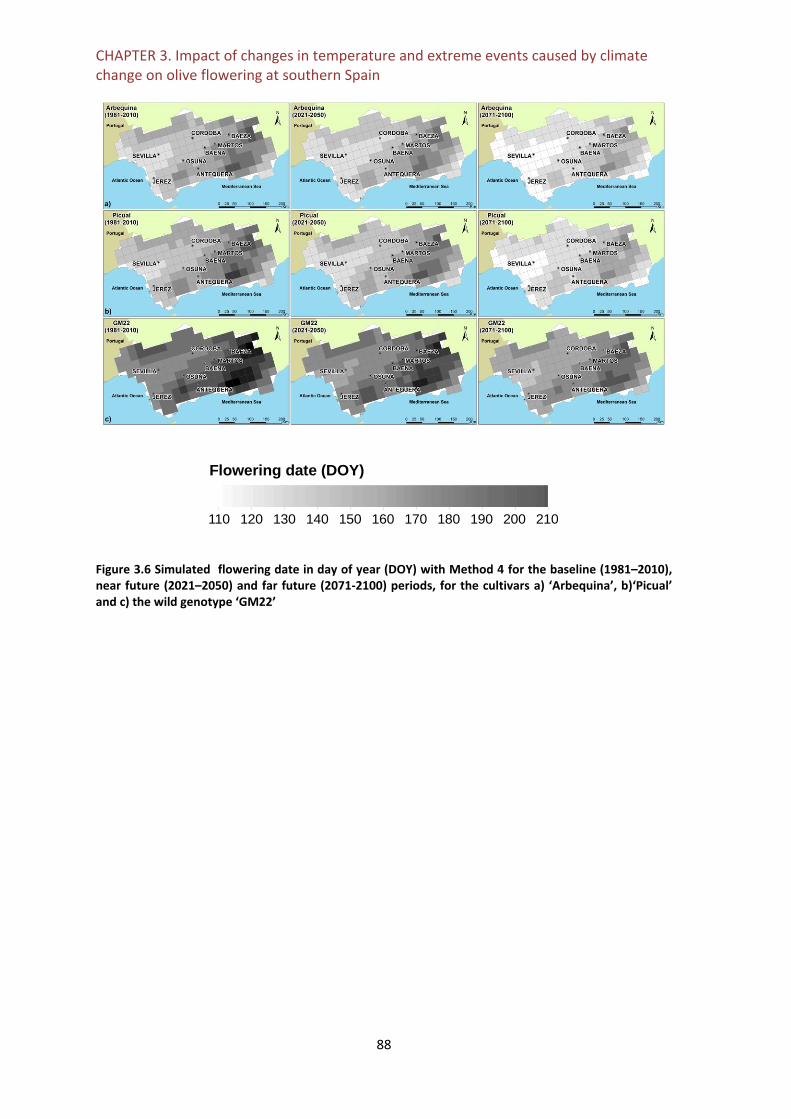
CHAPTER 3. Impact of changes in temperature and extreme events caused by climate change on olive flowering at southern Spain
88
Figure 3.6 Simulated flowering date in day of year (DOY) with Method 4 for the baseline (1981–2010), near future (2021–2050) and far future (2071-2100) periods, for the cultivars a) ‘Arbequina’, b)‘Picual’ and c) the wild genotype ‘GM22’
Flowering date (DOY)
210200190180170160150140130120110

CHAPTER 3. Impact of changes in temperature and extreme events caused by climate change on olive flowering at southern Spain
89
Table 3.3. Mean flowering date, for the cultivars ‘Arbequina’ and ‘Picual’ and the wild genotype ‘GM22’ at the selected locations for the baseline (1981–2010), near future (2021–2050) and far future (2071-2100) periods. The values in parenthesis are the coefficient of variation (CV, %) of the flowering dates projected by the 12 climate models considered. DOY: day of year.
Location
Arbequina Picual GM22
B NF FF B NF FF B NF FF
-----------------------------------------DOY-------------------------------------
Jerez 127 (0.3) 123 (1.4)
116 (1.7)
130 (0.3)
126 (1.4)
119 (1.7)
155 (0.4)
150 (1.2)
141 (1.7)
Seville 127 (0.4) 123 (1.4)
116 (1.9)
130 (0.4)
126 (1.4)
118 (1.9)
154 (0.5)
149 (1.2)
139 (1.9)
Osuna 134 (0.4) 129 (1.5)
121 (2.0)
137 (0.4)
132 (1.4)
124 (2)
161 (0.4)
156 (1.2)
145 (1.9)
Antequera 142 (0.6) 137 (1.8)
127 (2.3)
146 (0.6)
140 (1.8)
130 (2.3)
171 (0.5)
165 (1.4)
153 (2.3)
Cordoba 132 (0.5) 128 (1.5)
119 (2.2)
135 (0.5)
131 (1.5)
122 (2.2)
159 (0.5)
153 (1.3)
143 (2.1)
Baena 137 (0.5) 133 (1.4)
124 (2.2)
140 (0.5)
135 (1.4)
127 (2.2)
164 (0.4)
158 (1.2)
147 (2.1)
Martos 140 (0.5) 135 (1.5)
126 (2.3)
143 (0.5)
138 (1.5)
129 (2.3)
166 (0.4)
160 (1.3)
149 (2.3)
Baeza 148 (0.6) 143 (1.7)
131 (2.6)
151 (0.5)
145 (1.7)
134 (2.5)
174 (0.4)
167 (1.3)
155 (2.5)
3.3.4. Extreme temperature events
Once flowering dates were obtained, an analysis of the occurrence of extreme
events during this stage was carried out for Arbequina cultivar, the genotype with the
lowest GDD requirements for flowering, and GM22, the wild genotype with the highest
GDD requirements (Table 3.1).
The results for the whole Andalusia region show an increase in the occurrence of
heat extreme events per year for both 1-day and 3-days duration events (see section
3.2.5) (Fig. 3.7 and 3.8). For ‘Arbequina’ the mean occurrence of at least one hs1d-30
event by year increased around 19 and 38 % for NF and FF periods, respectively,
compared with B period (Table 3.4), being in North-North East the areas with the highest
occurrence of both hs1d-30 and hs3d-30 events. When a higher threshold temperature

CHAPTER 3. Impact of changes in temperature and extreme events caused by climate change on olive flowering at southern Spain
90
was considered (hs1d-35 and hs3d-35 events) the occurrence was lower (about the half
than for events with temperatures higher than 30°C), showing equally the highest
frequencies of occurrence in the North-Eastern area. Finally, for hs1d-40 events the
highest occurrence was around 10 % for FF period and was also found in the North-
Eastern area, while the occurrence of hs3d-40 events was null.
For ‘GM22’ the occurrence of heat extreme events was higher than for the rest of
cultivars and wild olive genotypes (Fig. 3.8, Table 3.4). The mean occurrence of at least
one hs1d-30 and hs3d-30 events by year increased around 9 and 22 %, respectively, for
the FF period compared with the B period, with maximum occurrences for hs1d-30
events close to the 100 % in North-North East area (e.g. Baeza location) for the three
considered periods (Table 3.4).
Regarding the hs1d-35 and hs3d-35 events, the mean number of events and the
percentage of years with occurrence was smaller than 30 °C threshold was considered.
The occurrence of at least one of these events (hs1d-35 and hs3d-35) increased in FF
period compared with B (around 46 and 83%, for hs1d-35 and hs3d-35 respectively) with
the maximum occurrences located in North-North East area (Baeza location). Finally, for
hs1d-40 and hs3d-40 events the occurrence in FF period varied significantly throughout
the region, with the highest occurrences projected for FF at the North-East of the region
(e.g. for Baeza location 47.7 and 21.1 % for hs1d-40 and hs3d-40 events, respectively), in
the upper section of Guadalquivir River.
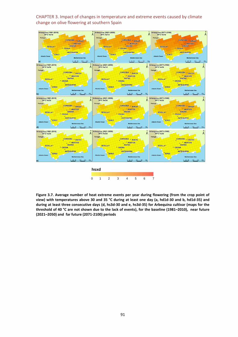
CHAPTER 3. Impact of changes in temperature and extreme events caused by climate change on olive flowering at southern Spain
91
Figure 3.7. Average number of heat extreme events per year during flowering (from the crop point of view) with temperatures above 30 and 35 °C during at least one day (a, hd1d-30 and b, hd1d-35) and during at least three consecutive days (d, hs3d-30 and e, hs3d-35) for Arbequina cultivar (maps for the threshold of 40 °C are not shown due to the lack of events), for the baseline (1981–2010), near future (2021–2050) and far future (2071-2100) periods
76543210
hsxd

CHAPTER 3. Impact of changes in temperature and extreme events caused by climate change on olive flowering at southern Spain
92
Table 3.4. Percentage of years with at least one event for one (hs1d) and three consecutive (hs3d) days above 30, 35 or 40 degrees during the flowering phase, for the cultivar ‘Arbequina’ and the wild genotype ‘GM22’, for the baseline (B, 1981–2010), near future (NF, 2021–2050) and far future (FF, 2071-2100) periods.
Arbequina
hs1d-30 (%) hs1d-35 (%) hs1d-40 (%) hs3d-30 (%) hs3d-35 (%) hs3d-40 Location code B NF FF B NF FF B NF FF B NF FF B NF FF B NF FF
Jerez A 31.4 41.1 54.1 0.3 1.9 7.4 0.0 0.0 0.0 8.9 13.3 26.5 0.0 0.0 1.4 0.0 0.0 0.0
Seville B 49.4 58.9 67.4 3.1 8.3 16.5 0.0 0.0 0.6 21.9 30.3 43.2 0.8 0.6 4.5 0.0 0.0 0.3
Osuna C 41.1 53.9 63.7 2.5 4.4 10.2 0.0 0.3 0.0 11.9 23.9 35.1 0.0 0.0 1.5 0.0 0.0 0.0
Antequera D 8.6 19.2 37.6 0.0 0.8 1.6 0.0 0.0 0.0 0.0 3.9 9.0 0.0 0.0 0.3 0.0 0.0 0.0
Cordoba E 61.4 70.3 78.6 8.6 16.9 27.0 0.3 0.3 1.2 28.3 41.4 47.3 0.6 3.1 9.2 0.0 0.0 0.3
Baena F 61.1 74.4 78.6 11.4 20.3 34.5 0.0 1.4 2.3 30.8 41.1 55.3 1.7 5.6 10.3 0.0 0.6 0.0
Martos G 70.3 77.8 84.8 16.1 29.2 47.1 0.3 2.2 4.2 35.0 45.6 63.7 3.9 8.3 14.7 0.0 0.8 0.3
Baeza H 78.9 81.9 90.5 30.6 37.5 55.8 1.9 3.9 10.3 46.4 55.3 67.4 7.5 12.5 20.7 0.0 0.3 0.9
mean 50.3 59.7 69.4 9.1 14.9 25.0 0.3 1.0 2.3 22.9 31.8 43.4 1.8 3.8 7.8 0.0 0.2 0.2
GM22
hs1d-30 (%) hs1d-35 (%) hs1d-40 (%) hs3d-30 (%) hs3d-35 (%) hs3d-40 Location B NF FF B NF FF B NF FF B NF FF B NF FF B NF FF
Jerez A 73.6 83.9 92.6 15.6 25.3 42.8 0.0 0.6 3.0 45.0 53.6 70.8 1.7 4.2 15.5 0.0 0.0 0.3
Seville B 88.9 91.1 98.0 37.2 50.6 66.5 1.4 1.9 14.7 61.1 67.2 84.2 12.5 20.0 36.6 0.0 0.0 2.4
Osuna C 87.2 89.7 95.3 20.6 30.6 49.6 0.3 1.1 2.7 61.1 66.9 79.7 3.6 8.1 21.4 0.0 0.0 0.3
Antequera D 70.0 75.0 85.4 5.6 11.7 22.0 0.0 0.0 0.3 31.1 34.7 48.9 0.8 1.1 4.9 0.0 0.0 0.0
Cordoba E 92.2 95.6 99.4 56.1 61.4 79.6 1.4 7.2 24.9 75.0 81.1 92.6 22.2 31.7 49.8 0.3 1.1 9.3
Baena F 97.2 96.1 99.0 65.3 66.9 79.9 6.4 13.6 30.4 83.1 83.1 89.4 33.6 37.2 52.6 0.6 4.2 12.0
Martos G 96.9 97.5 99.2 73.9 71.4 84.5 12.8 18.6 35.2 87.2 85.0 89.1 44.2 47.5 55.0 1.7 5.3 15.4
Baeza H 98.3 98.6 99.5 78.3 84.2 90.2 18.6 26.9 47.7 89.2 89.2 95.4 46.1 55.8 64.6 4.7 8.6 21.1
mean 88.1 90.9 96.1 44.1 50.2 64.4 5.1 8.7 19.9 66.6 70.1 81.3 20.6 25.7 37.6 0.9 2.4 7.6

CHAPTER 3. Impact of changes in temperature and extreme events caused by climate change on olive flowering at southern Spain
93
Figure 3.8. Average number of heat extreme events per year during flowering (from the crop point of view) with temperatures above 30, 35 and 40 °C during at least one day (a, hs1d-30, b, hs1d-35 and c, hs1d-40) and during at least three consecutive days (d, hs3d-30, e, hs3d-35 and f, hs3d-40) for ‘GM22’ wild genotype for the baseline (1981–2010), near future (2021–2050) and far future (2071-2100) periods
76543210
hsxd

CHAPTER 3. Impact of changes in temperature and extreme events caused by climate change on olive flowering at southern Spain
94
3.3.5. Vulnerability and alternative suitable areas for olive
cultivation at southern Spain
Combining the maps of percentage of years when the mean threshold of
chilling requirements were not achieved and the maps of percentage of years with at
least one event of one day with Tmax above 35°C during B and FF period (Supplement,
Fig A.3), a spatial analysis evaluating the flowering threats were defined (Fig. 3.9).
Overlapping these threat maps with the current cultivated olive areas in Andalusia, the
olive areas with the highest vulnerability to climate change as well as new areas
suitable for olive cultivation with the analysed genotypes (Fig. 3.9) arose. Thus,
considering ‘Arbequina’ and ‘Picual’ cultivars for the future period, the areas AOC and
SE (Southeast) were those with the highest vulnerability due to the lack of chilling
units. Similarly the areas located at NW (Northwest), North (N) and NE (Northeast)
were the most vulnerable to high temperature during flowering for the FF period (Fig.
3.9). These areas are larger and with higher percentage of years with at least one
event of one day with Tmax above 35 °C than for B period (Supplement A.3). In the
opposite case, the areas with the lowest vulnerability to extreme events were N-NW
(North-Northwest) and the S (South) for ‘Arbequina’. The areas with low vulnerability
were reduced for ‘Picual’, being limited to the Southern area. Finally, the wild
genotype ‘GM22’ was the cultivar most vulnerable to high temperatures during
flowering for both B and FF periods. However the percentage of years with at least one
event of one day with Tmax above 35 °C was lower in the B than the FF period
(Supplement A.3). The suitable areas were smaller to those determined for the rest of
genotypes, being limited to the S-SE (South-Southeast) and S areas (Fig. 3.9).
Using similar methodology, new areas suitable for the olive cultivation at the
end of the 21st century was identified. Thus, NW and S would be suitable areas for new
plantations for ‘Arbequina’ and ‘Picual’ cultivars as heat stress during flowering and
the possible lack of chilling units in winter were avoided. Equally, for the wild genotype
‘GM22’ the suitable area will be very limited to the S area of Andalusia (Fig. 3.9), due
to the higher incidence of heat stress events on flowering that the others cultivars.

CHAPTER 3. Impact of changes in temperature and extreme events caused by climate change on olive flowering at southern Spain
95
It should be noted that these areas were obtained evaluating two processes
independently, the lack of chilling hour accumulation and the heat stress during
flowering.
Lack chill: lack of chilling units; HSF: heat stress during flowering
Figure 3.9. Maps of vulnerable and suitable areas for olive cultivation, for the Arbequina, Picual, and GM22, for the baseline (1981–2010) and far future (2071-2100) periods.
3.4. DISCUSSION
Previous studies have shown the impact of the projected temperatures at the
end of the 21st century on the olive phenology considering simulation models
calibrated under baseline climate conditions (Osborne et al., 2000; Galán et al., 2005;
Avolio et al., 2012). Under these climate conditions, previous models such as the
developed by De Melo-Abreu et al. (2004) were validated using data from outdoors
experiments (OU) for ‘Arbequina’, ‘Hojiblanca’ and ‘Picual’ cultivars obtaining limited
differences between observed and simulated dates (2-5 days with Method 3) and
providing similar flowering dates (118 to 120 DOY) than those obtained in previous
studies (115-145 DOY by Fornaciari et al., 2000, 120-160 DOY by Osborne et al., 2000,
or 122-134 DOY by De Melo-Abreu et al., 2004). In spite of these consistent results
under baseline conditions, a huge variability in the calibration parameters was
Vulnerable
Lack chill HSF Lack chill/HSF
Suitable
Cultivated
No cultivated

CHAPTER 3. Impact of changes in temperature and extreme events caused by climate change on olive flowering at southern Spain
96
detected. Thus, Tb values reported by De Melo-Abreu et al. (2004), Galán et al. (2005),
Orlandi et al. (2005a, 2010a) or Aguilera et al. (2014), ranged from 5 to 23 °C, and the
lower and upper temperature thresholds for chilling accumulation requirements
described by De Melo Abreu et al. (2004), Orlandi et al. (2006) or Aguilera et al. (2014)
ranged from 5.2 to 7.3 °C and from 12 to 20.7 °C, respectively. This fact indicates the
difficulty to develop a general approach for estimating olive flowering date, even
under current climate conditions.
The accurate performance of the traditional phenology models when using
non-forced climate conditions (De Melo-Abreu et al., 2004) was significantly reduced
reproducing experimental data under forced climate, representing future conditions.
Thus, the approach that uniquely considered heat accumulation (without chilling
requirements) showed the best performance under forced climate conditions but still
the large difference between observed and simulated dates (ca. two weeks; Table 3.3)
implies that additional studies are required. This result defies our knowledge on the
quantity and even on the existence of chilling requirements for olive trees, in
agreement with some authors that reported a strong relation between uniquely the
flowering date and previous month’s temperature (Fornaciari et al., 1998; Galán et al.,
2005). Then, to develop alternative approaches for assessing climate change impacts
on crop phenology for Mediterranean olive orchards is still required. However the
development and local calibration of such models require experimental data under
forced climate conditions, which have been almost non-existent up to date.
In order to improve flowering date simulation under baseline and future
climate conditions, in this study a new model was developed and tested for ten olive
genotypes being locally calibrated using experimental data under baseline
(represented by the OU experiment) and forced (represented by the GH experiment)
climate conditions. The new approach provided very accurate results for both OU and
GH conditions, with differences between observed and simulated flowering date of
around 2 days and 3.9% for GDD (Table 3.1), with very low associated uncertainty. The
simulated flowering dates with the proposed approach for the B period considering all
the cultivars except the three wild genotypes (‘FV18’, ’GM22’ and ‘GM25’) showed a
large spatial variability within Andalusia, ranging from 125 DOY for the Atlantic Ocean

CHAPTER 3. Impact of changes in temperature and extreme events caused by climate change on olive flowering at southern Spain
97
Coast to 184 DOY for the East Mountains area. These values are within the range of
the published data by the Unit of Aerobiology at the University of Granada (RAA,
2015), obtained with pollen databases from 1992 to 2007. According to them, the
highest concentrations of olive pollen usually occurs during the second week of May
(134 DOY) in Almeria and Jaen provinces (Eastern Andalusia), while in the province of
Granada (South-Eastern Andalusia) the highest pollen concentration is delayed to the
third or fourth week of May (148 DOY) and even spans July (182 DOY) in the
mountainous areas. Analyzing flowering date by genotype, also significant variability
was found. Thus, the average flowering date in Cordoba for B period ranged from 132
for ‘Arbequina’ cultivar to 159 for the wild genotype ‘GM22’, with similar differences in
the rest of the region. When the wild olive genotypes were excluded, the differences
persisted but they were smaller, and were in agreement with De Melo-Abreu et al.
(2004). The proposed model was calibrated under two contrasting climate conditions
that encompassed the current and future climate conditions for the whole region of
Andalusia, supporting the application of the locally calibrated model to the rest of
Andalusia.
In spite of the impossibility to carry out a complete validation process due to
the limited number of climate conditions, the similar parameters determined for OU
and GH conditions in the calibration process demonstrated the high quality of the
proposed approach (Table 3.1). Equally, the analysis of sensitivity carried out for TU
indicated that for obtaining EDO values TU has not a critical importance. However the
percentage of years with flowering failure caused by lack of chilling requirements was
significantly impacted by the TU value, showing the necessity to promote studies
related with the accurate definition of this parameter, and agree with studies carried
out by Fornaciari et al. (1998) and Orlandi et al. (2004) that indicated the high
uncertainty when olive chilling requirements were estimated.
Advances in the flowering date were foreseen with the proposed approach for
the whole Andalusia region under future climate conditions. For FF period and within
the current olive cultivated areas in Andalusia, the average advance in flowering date
was equal to 17 days compared with the B period. This advance is in agreement to
Osborne et al. (2000) and Galán et al. (2005) who indicated advances in flowering date

CHAPTER 3. Impact of changes in temperature and extreme events caused by climate change on olive flowering at southern Spain
98
for olive of around 15-20 days. These results could be also partially validated taking
into account the temperature increase projected for March, April and May at the end
of the 21st century (around 2 °C; Fig. 3.3) and the relationship between temperature
increase and advance in the flowering date provided by Orlandi et al. (2010c),
identifying an advance in flowering date in Cordoba of around 15.2 days.
The use of an ensemble of bias corrected climate projections together with a
phenological model calibrated for local varieties has allowed the construction of
impact maps to identify vulnerable and potentially suitable areas for olive cultivation
in future, as well as to assess the uncertainty of the flowering date estimations. The
generation of these maps has been frequent (Ponti et al., 2014; Tanasijevic et al.,
2014) although the lack of local calibration, the absence of uncertainty assessment and
the reduced number of olive cultivars analysed has limited their applicability.
Thus, this study allowed identifying the most vulnerable and suitable cultivated
areas for baseline and future conditions. The spatial analysis of the vulnerable areas by
the lack of chilling units (TU) considering high chilling requirements for olive identified
the AOC and the SE coast areas are the most susceptible. However, according with the
farmers experience and the aggregated reported yields for the AOC area (CAPDR,
2016b), problems associated to the lack of chilling hour requirements have not been
found. These results encourage considering low TU values for future impact
assessment. In relation with uncertainty, for EDO date projections this was very low
(CV values below 3% whenever the period and location), although in this value
uniquely uncertainty associated to RCMs under the same emission scenario (SRES-A1B)
(Hawkins and Sutton, 2009; Dosio et al., 2012) was considered.
The frequency of occurrence of heat extreme events during olive flowering
increased under future climate conditions, identifying the North-Northeast area as the
most vulnerable to climate change due to the high temperatures during flowering.
Within this area, the percentage of occurrence of at least one event during the
sensitive flowering period with temperatures above 35 °C for ‘Arbequina’ was around
38 and 56 % during NF and FF periods, respectively. This trend is in agreement with
previous studies that shows an increase in the number of extreme temperature events
for both global (Tebaldi et al., 2006; Teixeira et al., 2013) and Europe level (Beniston et

CHAPTER 3. Impact of changes in temperature and extreme events caused by climate change on olive flowering at southern Spain
99
al., 2007). Olive cultivars with later flowering (such as ‘GM22’ genotype) had a higher
exposure to extreme events. Thus, for the same area the frequency of occurrence of at
least one heat event during the sensitive period of flowering with temperatures above
35 °C for ‘GM22’ was around 84 and 90 % during NF and FF periods, respectively, and
therefore a more severe impact of climate change would be foreseen.
As vulnerability related with heat extreme events varied significantly between
cultivars and locations, this should be taken into account for an adequate cultivar
selection at a specific location avoiding late cultivars in areas with frequent foreseen
heat extreme events. The consideration of the extreme events during the simulated
flowering period is a recent and useful methodology (Ruiz-Ramos et al., 2011, Eitzinger
et al., 2013, Teixeira et al., 2013; Trnka et al., 2014). However, this methodology is
affected by uncertainties such as the accurate estimation of the length of the flowering
sensitive period for olive that could be reduced due to the effect of high temperatures
(Vuletin Selak et al., 2014), or by the unawareness of the impact of heat extreme
events during flowering specifically for olive. Thus, contrary to other crops as
sunflower (García-Lopez et al. 2014) or maize (Gabaldón-Leal et al., 2015), the
available information about these impacts on olive is very limited. To solve this
knowledge gap, extensive experimental studies for understanding and quantifying the
impacts of these events on olive are still required.
Adaptation strategies for Mediterranean olive orchards to avoid the lack of
chilling units for sensitive areas such as AOC area were very limited, and severely
affected by the high uncertainty caused by the lack of knowledge for chilling
requirements by genotype. Similarly, adaptation strategies to reduce the impact of the
foreseen heat stress events in the near future would be the selection of cultivars with
early flowering date, the use of cover crops and soil management practices to modify
the albedo to reduce air temperature (Davin et al. 2014), or the consideration of
supplementary irrigation to reduce the olive canopy temperature (Doughty et al.,
2011; Andrade et al., 2012). Equally, new suitable areas for olive cultivation could be
extended in the NW and S areas of Andalusia for ‘Arbequina’ and ‘Picual’ cultivars.
Finally, the proposed methodology has been designed for olive orchards under
the semi-arid conditions of Southern Spain and has only taken into account changes in

CHAPTER 3. Impact of changes in temperature and extreme events caused by climate change on olive flowering at southern Spain
100
both mean and maximum temperatures, regardless of changes in rainfall and the soil
moisture content. The impact of water stress on olive, promoted by the foreseen
climate models of Andalusia region, will have similar relevance on olive yield and
studies related with this must be promoted.
Although this study has been focused on olive for Southern Spain conditions,
the proposed methodology of using greenhouses to reproduce the projected climate
could be applicable for other crops and locations. Thus, the described methodology
could be replicated to assess the impact of climate change on others Mediterranean
crops such as nut or fruit trees.
3.5. CONCLUSION
This study has evaluated the olive flowering date for ten olive genotypes (seven
traditional cultivars in southern Spain and three olive genotypes from Canary Islands)
under baseline and future climate conditions. Validation of previous phenological
models for flowering date estimation and the development of a new approach
adapted to both baseline and projected climate conditions, were carried out
considering experimental data. The study was carried out in Andalusia region, located
at Southern Spain and considered an ensemble of climate projections from Regional
Climate Models (RCMs) with a bias correction in temperature and precipitation. From
these simulations, an advance in the flowering date of around 6 and 17 days for 2021-
2050 and 2071-2100 periods, respectively, compared with 1981-2010 period was
projected. The uncertainty associated to these phenological projections coming from
climate projections was very low.
The integration of local experimentation, phenological modelling and climate
data from an ensemble of climate throughout Andalusia region allowed developing a
spatial analysis of the impacts of climate change on olive flowering and its uncertainty.
This analysis was based on the estimation of the flowering date, the chilling hour
accumulation and the occurrence of heat extreme events during the flowering stage
for ten olive genotypes. We concluded in the identification of those areas more

CHAPTER 3. Impact of changes in temperature and extreme events caused by climate change on olive flowering at southern Spain
101
vulnerable to climate change (such as the Atlantic Ocean Cost and Northern-East areas
of Andalusia) and those potential new areas for olive cultivation (such as the North-
West and South area). Late flowering cultivars (such as wild olive genotypes from
Canary Islands) were the most vulnerable ones to high temperatures during flowering.
This study highlights the need to promote experimental studies on crop
physiology and phenology under future climate conditions to improve the knowledge
about the response of Mediterranean olive orchards to climate change. The described
methodology is not exclusive for the olive crop and could be replicated to assess the
impact of climate change on others crops and locations.
Acknowledgments
This study has been financially supported by the project RTA2014-00030-00-00
funded by INIA, FEDER 2014-2020 “Programa Operativo de Crecimiento Inteligente”,
FACCE MACSUR – Modelling European Agriculture with Climate Change for Food
Security, a FACCE JPI knowledge hub, by AGR-6126 project funded by the Consejería de
Innovación, Ciencia y Empresa (Junta de Andalucía) and by MULCLIVAR, from the
Spanish Ministerio de Economía y Competitividad (MINECO) CGL2012-38923-C02-02.
Appendix. Supplementary data
Supplementary material related to this article can be found in Annex.

102

GENERAL DISCUSSION
103
GENERAL DISCUSSION
This Thesis has addressed the impacts of climate change on maize and olive
crops under semi-arid conditions in Andalusia region. In addition, the incidence of
extreme temperature events on flowering, a sensitive phenological period for
numerous crops to high temperatures (Koubouris et al., 2009; Gourdji et al., 2013), has
been evaluated for both crops. Thus, a model to evaluate the impact of heat stress
events during flowering on maize yield has been provided, trying to mitigate the
limitations found in current maize grain yield modeling under these conditions (Rezaei
et al., 2015). Also for maize, considering modeling tools, possible adaptation strategies
were proposed and evaluated in order to minimize the described impacts.
The Thesis is based on the development and use of crop simulation models for
the assessment of impacts and adaptation strategies considering the effect of extreme
maximum temperatures on the crops. The methodology considers experimental data
for local calibration and validation under current and forced climate conditions, being
essential this experimentation in order to adjust the model to the future climate
regional conditions, with the purpose of generating projections at local and regional
scale (Boote et al. 2013). The consideration of experimental data, together with the
use of a bias corrected ensemble from regional climate models, has provided future
projections with lower uncertainty than previous studies. However further
experimental studies are still needed. Thus, in this study uniquely changes in both
mean and maximum temperatures has been evaluated, and then changes in rainfall
and the soil moisture content have not been considered. The integration of heat and
water stress impacts in the crop models will provide a more accurate evaluation of
climate change impacts on Mediterranean agriculture.
Future climate projections show an increase in future temperatures, being
particularly important for Andalusia region, at southern Spain, with an increase in
mean temperature up to 5 °C in the summer months (Van der Linden and Mitchel,
2009). Furthermore an increase in the frequency and magnitude of heat extreme
events is projected worldwide with climate change (Tebaldi et al., 2006; Field et al.,
2012), again with a higher increase at southern Spain (Sánchez and Miguez-Macho,
2010). This increase would probably lead to a larger incidence of heat stress for crops

GENERAL DISCUSSION
104
compared to current conditions (Schlenker and Roberts, 2009; Lobell et al., 2013;
Trnka et al., 2014).
Under future climate conditions, advancement in phenological dates was
projected for both maize crop and olive trees, due to the higher temperatures
projected at the end of 21st century (IPCC, 2014). These results were obtained using
crop models calibrated under local conditions, with errors detected in the calibration
of the maize crop model similar than those obtained in previous studies (Meza et al.,
2008; Vučetić, 2011; Angulo et al., 2013; Moradi et al., 2013). The impacts of future
climate conditions using these models showed a shortening in the maize crop cycle,
similar to the results observed by Olesen et al. (2012) and Bassu et al. (2014) in cereals,
including maize. These changes lead to projections of maize yield decrease for
locations along the Guadalquivir River basin, although smaller than the indicated in
previous studies (Guereña et al. 2001; Garrido et al. 2011 and Rey et al. 2011). For
some locations as Granada, located in the Southern part of Andalusia and nearby
Sierra Nevada mountains, the decrease in yield was more severe due to the reduction
in crop cycle was higher than for the other locations. Similarly, the impacts of extreme
temperature events on maize during flowering were evaluated following Teixeira et al.
(2013) for Andalusia region, showing an increase in the heat stress index, causing a
higher production damage index at the end of the 21st century.
Another important impact for maize crop in Andalusia is regarding the irrigation
requirements (IRR) and the irrigation water productivity (IWP). The results showed a
decrease in the estimated IRR for future periods for all the locations. This decrease
could be explained by the reduction of the crop cycle duration and the crop
evapotranspiration, caused by warmer temperatures and the reduced stomatal
conductance as consequence of future CO2 concentrations (Cure and Acock 1986;
Ainsworth and Long 2005). The increased IWP in the future periods could be related to
the described reduction on stomatal conductance (Leakey et al. 2006; Vanuytrecht et
al. 2012).
The projection results for maize yield under future climate conditions were
evaluated for five locations, four of them along the Guadalquivir river basin, showing
similar results and low uncertainty. This low uncertainty exhibited by the projections is
partially as consequence of conducting simulations under an optimum irrigation

GENERAL DISCUSSION
105
supply, which excludes the uncertainty linked to precipitation. The precipitation
uncertainty is usually higher than for other variables (Christensen and Christensen,
2007) due to the spatially and temporally complex structure and its related physical
processes, being especially large in the Iberian Peninsula (Sánchez and Miguez-Macho,
2010). However, Granada area showed higher uncertainty than the Guadalquivir
locations expressed as the spread of the ensemble members or differences among
RCM outputs. In turn, these differences could be enhanced by the complex orography
of Granada area. For instance, while mean altitude for the Guadalquivir Valley
locations is 100 m a.s.l, Granada is at 633 m a.s.l. For this particular location, its actual
altitude is lower than the mean grid altitude of 1034 m considered by both the
observational data set E-OBS and the ensemble of corrected RCM projections ENS-
EOBS; this misrepresentation of altitude would introduce an error and contribute to
the accumulated uncertainty.
Impacts on olive trees were studied in relation to the flowering date
assessment under current and future climate conditions and the occurrence of
extreme events during this critical phenological stage. The new approach provided
very accurate results for both current (evaluated by experiments under current actual
conditions) and forced conditions (considering experiments placed inside a greenhouse
reproducing the future climate conditions), with differences between observed and
simulated flowering date of around 2 days and with very low associated uncertainty.
The simulated flowering dates projected for the baseline period (1981-2010) showed a
significant spatial variability within Andalusia (125-184 DOY). These results are in the
range of the published data by the Unit of Aerobiology at the University of Granada
(RAA, 2015), that found the highest concentrations of olive pollen during the second
week of May in the Eastern areas of Andalusia, and up to July in the mountainous
areas.
For flowering date estimation in olive, the fulfillment of chilling requirement (or
end of endormancy) has a critical importance (Rallo and Martin, 1991). Analyzing this
fulfillment for the whole Andalusia region at the end of the 21st century, the most
susceptible areas to lack of chilling requirements accumulation were the Atlantic
Ocean and South East Coasts. The results related with the lack of chilling units for olive
obtained are in agreement with the yield reports provided by farmers and public

GENERAL DISCUSSION
106
institutions for the last years in the Atlantic Ocean Coast area, which did not detect
problems of lack of chilling hour requirements (CAPDR, 2016b).
For olive trees the impact of extreme temperature events was evaluated using
a similar approach than Ruiz-Ramos et al. (2011), considering number of events during
flowering period with temperature above different thresholds. The frequency of
occurrence of heat extreme events during olive flowering under projected future
climate conditions generally increased with very low uncertainty, with the highest
frequency in the North-Northeast area of Andalusia. The increasing trend projected
was in agreement with previous studies developed by Tebaldi et al. (2006), Beniston et
al. (2007), Ruiz-Ramos et al. (2011) and Teixeira et al. (2013). In the study, differences
in vulnerability between cultivars and locations were found and should be taken into
account for an adequate cultivar selection at a specific location, avoiding late cultivars
(such as the wild genotype GM22) in areas with frequent foreseen heat extreme
events (such as North-Northern areas of Andalusia).
The general very low uncertainty associated to the olive crop results was due to
the fact that the impacts projections were based only in temperature, variable with
lower uncertainty than the precipitation, as mention above. Also, in this study the
ensemble of climate models used was ENS-Spain02, especially developed for impact
assessment (Ruiz-Ramos et al., 2015). In spite of the low uncertainty detected, this one
was slightly higher for future periods compared with the baseline due to inherent
uncertainty of the climate models and was in agreement to Ferrise et al. (2011) and
Hoffmann and Rath (2013).
It should be noted that the uncertainty evaluated was only that caused by
differences in the projections provided by the RCMs under the same emission scenario
(SRES-A1B) (Hawkins and Sutton, 2009; Dosio et al., 2012). This is one of the largest
uncertainty sources in climate change impact assessment as Iglesias et al. (2010) for
olive, Hoffmann and Rath (2013) for apple, Ruiz-Ramos and Mínguez (2010) and
Asseng et al. (2013) for wheat and maize described. However there are other relevant
uncertainty sources not addressed here, as driving GCM, climate scenarios and others
decisions related to climate (Déqué et al, 2007). Equally, uncertainty coming from crop
models must be considered and it has arisen as an important uncertainty source
(Asseng et al., 2015).

GENERAL DISCUSSION
107
The methodologies used reduce the uncertainty of impact projections
improving several uncertainty sources. First, the uncertainty coming from climate
model outputs is reduced by the use of regional climate models (RCMs) instead of
general climate models (GCMs) providing climate information at the required scale (ca.
5 to 50 km for RCMs vs. 100 to 200 km for GCMs) for local and regional assessments, in
areas with complex orography as Andalusia (Guereña et al., 2001). Additional steps for
reducing the uncertainty were 1) the use of an ensemble of RCMs instead of a single
one projection, to consider the uncertainty from climate model parameterization
(Christensen et al., 2007; Semenov and Stratonovitch 2010), and 2) the use of the bias
corrected temperature and precipitation ensemble members. Thus, more specifically,
two bias corrected climate datasets from the ENSEMBLES European project were used;
one of them based on the observational E-OBS dataset, with 2316 stations covering all
Europe (50 of them in Spain) (ENS-EOBS) and the second one, using as observational
reference a dataset specifically generated for continental Spain and the Balearic
Islands based on 2756 quality-controlled weather stations (Spain02, Herrera et al,
2012). For both climate datasets a bias correction in temperature and precipitation
following (Dosio and Paruolo, 2011) and delivered by Ruiz-Ramos et al. (2015) (ENS-
Spain02) was considered. These improvements resulted in an overall reduction of
uncertainty when compared to former studies (Ruiz-Ramos and Mínguez, 2010; Ruiz-
Ramos et al., 2015).
The adaptation strategies for maize tested, such earlier sowing dates, or
cultivar changes with longer and more effective grain filling period have proven to
diminish negative impacts at field, regional, and European levels (Olesen et al. 2011).
However, our results emphasize that the adaptations for these events must be local,
due to differences in the spatial pattern of extreme events (Teixeira et al. 2013) and
local cropping system features. The adaptations proposed for maize to deal with climate change impacts were
an earlier sowing date, in agreement with Moriondo et al. (2011), combined with
cultivar changes searching for a longer grain filling period (Tollenaar and Lee 2011;
Chen et al. 2013; Ning et al. 2013). The combination of both strategies, sowing dates
and improved cultivars yielded the best projection results and are feasible from the
breeding and management points of view. With this combined adaptation the

GENERAL DISCUSSION
108
potential yield were recovered in all the locations, and even increased in the
Guadalquivir locations.
When impacts and adaptation strategies are evaluated, it is required to
consider that actual yield would be lower than the simulated, as the simulations did
not include any biotic nor abiotic stresses. Thus, if the effects of extreme maximum
temperatures during flowering are considered, in some locations as Granada the yield
would still remain around 8 % below current level, even when the adaptation is
applied. This aspect stresses the importance of the lack of heat stress consideration by
crop models.
When the adaptation strategies were considered irrigation requirements, IRR,
were lower for future periods compared with the baseline period. This reduction was
due to the earlier maturity dates, avoiding the crop the driest and hottest periods.
Equally, with the adaptations implemented, irrigation water productivity also
increased because yield increased more than crop transpiration and IRR, which implies
that the adaptations are useful not only for increasing or maintaining crop yields, but
for saving water and use it efficiently.
Adaptation strategies for Mediterranean olive orchards to reduce the impact of
heat stress on olive in the near future are less numerous than for crops as maize, and
would be limited to the selection of cultivars with early flowering date (such as
Arbequina or Koroneiki), the use of cover crops and soil management practices to
modify the albedo to reduce air temperature (Davin et al. 2014), or the consideration
of supplementary irrigation to reduce the olive canopy temperature (Doughty et al.,
2011; Andrade et al., 2012). An additional adaptation strategy would be the selection
of new suitable cultivation areas. Thus, new suitable areas for olive cultivation could
be extended in the North-West and South areas of Andalusia region for Arbequina and
in the Southern areas for Picual.
After the evaluation of the available crop and phenological models for impact
and adaptation strategies assessment, a very significant knowledge gap has been
detected for olive crop, contrasting with the available crop models for wheat, maize
and other field crops. Thus, key processes such as chilling requirements or heat
accumulation must be correctly simulated to make possible a reliable modeling of olive
yield formation and therefore, crop yield estimation. Aware of these limitations

GENERAL DISCUSSION
109
previous approaches have been evaluated and a general approach has developed for
estimating olive flowering date. The results obtained showed a good fit with the
flowering dates for baseline and future conditions, so the new approach was adequate
for generating projections of flowering dates under future climate conditions.
However, not only olive crop has limitations in the development of approaches for
evaluating key components for identifying the effect of climate change on crops. Thus,
crop models must be improved to consider the effects of heat stress for both large
(Ewert et al., 2015; Rezaei et al., 2015) and local scales. For that reason the simulation
of maize grain yield under heat stress conditions has been evaluated.
A heat stress model has been developed and evaluated in order to simulate
maize grain yield under heat stress conditions around silking, obtaining satisfactory
performance. Thus, a heat stress reduction factor was obtained using experimental
data from Argentine and validated with experimental data from Spain, being
appropriate for using under climate change conditions. The model performance was
improved when canopy temperature was considered as input for the heat stress
function instead of air temperature. To use air temperature as input, the critical
threshold must be increased from 34 °C, determined by Cicchino et al. (2010), to 39 °C
as this critical threshold could be several degrees higher under irrigation conditions
due to the irrigation cooling effect (Lobell et al., 2008; Kimball et al., 2015). The
improvement in crop modeling for maize and olive crops has accomplished and
demonstrated the need to promote experimental studies on crop physiology and
phenology under forced conditions to increase the knowledge about the response of
different Mediterranean crops to climate change. Furthermore, the importance of
access to high quality experimental data, to calibrate and validate crop models under
local and forced climate conditions has addressed. The collaboration between
modellers and experimentalist has been proved to be useful. In addition, the
development of specific experimental designs to feed the crop models to evaluate
future climate conditions, as heat events or water deficits under different phenological
phases for maize, olive or other crops, is recommended.
Several further maize model improvements could be desirable. Among them, to
examine the correlation between hourly heat stress and radiation use efficiency under
high temperatures. Furthermore the evaluation of the canopy temperature model

GENERAL DISCUSSION
110
under rainfed conditions could be useful, as uniquely under irrigated conditions has
been analyzed. This evaluation under different conditions could improve the model
applicability across different climate regions and management options. Regarding the
olive model, a complete phenological characterization under different climate
conditions, as warmer winters, could be useful to parametrize the chilling
requirements and phenological stages. Furthermore an evaluation of the temperature
profile along the olive tree could be useful to evaluate the impact of high temperatures
during flowering under irrigation or rainfed conditions, as well as evaluating the
flowering quality after high temperature exposure during flowering. Finally, the
accurate assessment of the impact of water stress during critical phenological stages as
flowering could provide a complete approach for determining the impact of climate
change on olive crop.
The study is in line with the Climate-smart agriculture (CSA) approach proposed
by FAO, as it is focused on the evaluation of the adaptations strategies to cope with
the impacts of climate change. In addition, the improvement of crop models for the
simulation of crop phenology and yield under heat stress conditions may contribute to
further research in the world regions with the largest food security challenges.
GENERAL CONCLUSIONS
111
GENERAL CONCLUSIONS
The present Thesis has confirmed that:
A reduction of uncertainty of impact and adaptation projections can be
achieved by combining 1) bias corrected, reduced uncertainty climate
projections, and 2) site-specific calibrated and validated crop models.
Considering the impacts of extreme events in reducing the crop yield is crucial
when assessing adaptations strategies. Crop models needs to be improved to
capture these effects.
The present Thesis has concluded that:
An irrigated maize yield reduction (6-20 %) is projected at the end of the 21st
century due to the shorter crop cycle that will cause crop evapotranspiration
reduction and an increase in heat stress events frequency.
Adaptation strategies such as earlier sowing dates and cultivar changes, when
they are locally addressed, have the potential to compensate and even increase
maize yields in Andalusia.
The irrigation requirements of maize at the end of the 21st century were
reduced around 25 % compared with the baseline period without adaptation
strategies due to the reduction in crop evapotranspiration and higher water use
efficiency. With the selected adaptation the decrease in the irrigation
requirements showed a limited decrease or it was slightly higher in Granada
compared to those without adaptation. This was due to the earlier maturity
dates, which allowed the crop to avoid the driest and hottest period for the
maize crop; however the irrigation requirements were still lower than those of
the baseline period.
Extreme temperature events during flowering may limit the effect of the
adaptation measures for maize in some areas of Andalusia (as Granada) due to
the later flowering date compared with the others locations studied.

GENERAL CONCLUSIONS
112
SIMPLACE <Lintul5,HS,Tc> model performed correctly in simulating grain yield
maize reductions based on the accumulated stress thermal time above a critical
threshold temperature during the critical period of flowering.
The SIMPLACE <Lintul5,HS,Tc> model performed better when canopy
temperature was used as input in the heat stress function.
When air temperature was considered for the critical threshold for heat stress
in SIMPLACE <Lintul5,HS,Tc> model, this threshold has to be increased from 34
°C (which is a physiologically meaningful threshold) to 39 °C (as the maize was
considerably cooler than the air due to ambient cooling caused by irrigation).
Increasing the critical temperature is an alternative option when air
temperature is considered in the heat stress reduction function under irrigated
conditions, but is not expected to be a suitable approach under rainfed
conditions due to the lack of irrigation cooling effect.
For olive flowering date estimation under climate change conditions a new
approach adapted to future climate conditions was proposed and evaluated.
For the entire Andalusia area, compared with 1981-2010 period, an advance in
the flowering date of around 6 and 17 days for 2021-2050 and 2071-2100
periods, respectively, was estimated.
These estimations for olive crop are robust due to the low associated
uncertainty.
The integration of local experimental data, phenological modelling and climate
data from an ensemble of climate models throughout Andalusia allowed
developing a spatial analysis of the impacts of climate change on olive
flowering.
Based on the estimation of the flowering date, chilling requirements and the
occurrence of extreme events during the flowering stage, identification of
vulnerable and potential new areas for olive cultivation was defined. Thus,
Atlantic Ocean area and South-East coast were found to be vulnerable due to
lack of chilling units in winter and the Northern-East region due to the high

GENERAL CONCLUSIONS
113
temperatures during flowering. Olive crop could be potentially extended to
new areas as the southern area in the future.
The described methodology is not exclusive for the olive crop and could be
replicated to assess the impact of climate change on others Mediterranean
crops such as nuts or fruit trees, requiring previous local calibration based on
field experiments.

114

GENERAL REFERENCES
115
GENERAL REFERENCES
Ainsworth, E.A., Long, S.P., 2005. What have we learned from 15 years of free air CO2 enrichment (FACE)? A meta-analytic review of the response of photosynthesis, canopy properties and plant production to rising CO2. New Phytol. 165, 351–372.
Allen, L.H., Kakani, V.G., Vu, J.C. V, Boote, K.J., 2011. Elevated CO2 increases water use
efficiency by sustaining photosynthesis of water-limited maize and sorghum. J. Plant Physiol. 168, 1909–1918.
Andrade, J.A., Vega, C., Uhart, S., Cirilo, A., Cantarero, M., Valentinuz, O., 1999. Kernel
number determination in maize. Crop Sci. 39, 453–459. Andrade, F.H., Echarte, L., Rizzalli, R., Della Maggiora, a., Casanovas, M., 2002. Kernel
number prediction in maize under nitrogen or water stress. Crop Sci. 42, 1173–1179.
Andrade, J.A., Santos, F.L., Correia, M., do Paço, T.A., 2012. Effects of Irrigation and
Tree Spacing on Soil and Air Temperature Profiles of Olive Orchards. VII Int. Symp. Olive Grow. 1057, 443–450.
Angelopoulos, K., Dichio, B., Xiloyannis, C., 1996. Inhibition of photosynthesis in olive
trees (Olea europaea L.) during water stress and rewatering. J. Exp. Bot. 47, 1093–1100.
Angulo, C., Rötter, R., Lock, R., Enders, A., Fronzek, S., Ewert, F., 2013. Implication of
crop model calibration strategies for assessing regional impacts of climate change in Europe. Agric. For. Meteorol. 170, 32–46.
Asseng, S., Ewert, F., Rosenzweig, C., Jones, J.W., Hatfield, J.L., Ruane, A.C., Boote, K.J.,
Thorburn, P.J., Rotter, R.P., Cammarano, D., Brisson, N., Basso, B., Martre, P., Aggarwal, P.K., Angulo, C., Bertuzzi, P., Biernath, C., Challinor, A.J., Doltra, J., Gayler, S., Goldberg, R., Grant, R., Heng, L., Hooker, J., Hunt, L.A., Ingwersen, J., Izaurralde, R.C., Kersebaum, K.C., Mueller, C., Kumar, S.N., Nendel, C., O’Leary, G., Olesen, J.E., Osborne, T.M., Palosuo, T., Priesack, E., Ripoche, D., Semenov, M.A., Shcherbak, I., Steduto, P., Stoeckle, C., Stratonovitch, P., Streck, T., Supit, I., Tao, F., Travasso, M., Waha, K., Wallach, D., White, J.W., Williams, J.R., Wolf, J., 2013. Uncertainty in Simulating Wheat Yields Under Climate Change. Nat. Clim. Chang. 3, 827–832.
Asseng, S., Ewert, F., Martre, P., Rötter, R.P., Lobell, D.B., Cammarano, D., Kimball, B.
A., Ottman, M.J., Wall, G.W., White, J.W., Reynolds, M.P., Alderman, P.D., Prasad, P.V. V., Aggarwal, P.K., Anothai, J., Basso, B., Biernath, C., Challinor, A. J., De Sanctis, G., Doltra, J., Fereres, E., Garcia-Vila, M., Gayler, S., Hoogenboom, G., Hunt, L. A., Izaurralde, R.C., Jabloun, M., Jones, C.D., Kersebaum, K.C., Koehler, A.-K., Müller, C., Naresh Kumar, S., Nendel, C., O’Leary, G., Olesen, J.E.,

GENERAL REFERENCES
116
Palosuo, T., Priesack, E., Eyshi Rezaei, E., Ruane, A. C., Semenov, M. A., Shcherbak, I., Stöckle, C., Stratonovitch, P., Streck, T., Supit, I., Tao, F., Thorburn, P.J., Waha, K., Wang, E., Wallach, D., Wolf, J., Zhao, Z., Zhu, Y., 2015. Rising temperatures reduce global wheat production. Nat. Clim. Chang. 5, 143–147.
Audsley, E., Pearn, K.R., Simota, C., Cojocaru, G., Koutsidou, E., Rounsevell, M.D.A.,
Trnka, M., Alexandrov, V., 2006. What can scenario modelling tell us about future European scale agricultural land use, and what not? Environ. Sci. Policy 9, 148–162.
Avolio, E., Pasqualoni, L., Federico, S., Fornaciari, M., Bonofiglio, T., Orlandi, F., Bellecci,
C., Romano, B., 2008. Correlation between large-scale atmospheric fields and the olive pollen season in Central Italy. Int. J. Biometeorol. 52, 787–796.
Barnabás, B., Jäger, K., Fehér, A., 2008. The effect of drought and heat stress on
reproductive processes in cereals. Plant, Cell Environ. 31, 11–38. Barriopedro, D., Fischer, E.M., Luterbacher, J., Trigo, R.M., García-Herrera, R., 2011.
The hot summer of 2010: redrawing the temperature record map of Europe. Science (80-. ). 332, 220–224.
Bassu, S., Brisson, N., Durand, J.L., Boote, K., Lizaso, J., Jones, J.W., Rosenzweig, C.,
Ruane, A.C., Adam, M., Baron, C., Basso, B., Biernath, C., Boogaard, H., Conijn, S., Corbeels, M., Deryng, D., De Sanctis, G., Gayler, S., Grassini, P., Hatfield, J., Hoek, S., Izaurralde, C., Jongschaap, R., Kemanian, A.R., Kersebaum, K.C., Kim, S.H., Kumar, N.S., Makowski, D., Müller, C., Nendel, C., Priesack, E., Pravia, M.V., Sau, F., Shcherbak, I., Tao, F., Teixeira, E., Timlin, D., Waha, K., 2014. How do various maize crop models vary in their responses to climate change factors? Glob. Chang. Biol. 20, 2301–2320.
Beniston, M., 2004. The 2003 heat wave in Europe: A shape of things to come? An
analysis based on Swiss climatological data and model simulations. Geophys. Res. Lett. 31.
Beniston, M., Stephenson, D.B., Christensen, O.B., Ferro, C.A.T., Frei, C., Goyette, S.,
Halsnaes, K., Holt, T., Jylhä, K., Koffi, B., Palutikof, J., Schöll, R., Semmler, T., Woth, K., 2007. Future extreme events in European climate: an exploration of regional climate model projections. Clim. Change 81, 71–95.
Bindi, M., Olesen, J.E., 2011. The responses of agriculture in Europe to climate change.
Reg. Environ. Chang. 11, 151–158. Bonofiglio, T., Orlandi, F., Sgromo, C., Romano, B., Fornaciari, M., 2008. Influence of
temperature and rainfall on timing of olive (Olea europaea) flowering in southern Italy. New Zeal. J. Crop Hortic. Sci. 36, 59–69.

GENERAL REFERENCES
117
Boogaard, H.L., van Diepen, C.A., Rötter, R.P., Cabrera, J.M.C.A., van Laar, H.H., 1998.
WOFOST 7.1. User’s Guide for the WOFOST 7.1 Crop Growth Simulation Model and WOFOST Control Center 1.5.52. DLO Winand Staring Centre, Wageningen, p. 142
Boote, K.J., Jones, J.W., Hoogenboom, G., Pickering, N.B., 1998. The CROPGRO model
for grain legumes. In: Tsuji, G.Y., et al. (Eds.), Understanding Options for Agricultural Production. Kluwer Academic Publisher, Dordrecht, The Netherlands, pp. 99–128.
Boote, K., Allen, L., Prasad, P.V.V., Baker, J., Gesch, R., Snyder, A., Pan, D., Thomas, J.,
2005. Elevated temperature and CO2 impacts on pollination, reproductive growth, and yield of several globally important crops. J. Agric. Meteorol. 60, 469-474.
Boote, K.J., Jones, J.W., White, J.W., Asseng, S., Lizaso, J.I., 2013. Putting mechanisms
into crop production models. Plant, Cell Environ. 36, 1658–1672. CAPDR, 2008. El Sector del Aceite de Oliva y de la Aceituna de mesa en Andalucía.
Consejería de Agriculuta, Pesca y Desarrollo Rural. Junta de Andalucía, Sevilla CAPDR, 2016a. Observatorio de precios y mercados. Productos industriales. Aceite de
oliva. Consejería de Agriculuta, Pesca y Desarrollo Rural. Junta de Andalucía, Sevilla (http://www.juntadeandalucia.es/agriculturaypesca/observatorio/servlet/FrontController?action=Subsector&table=3940&ec=subsector&subsector=33)(verified 10/01/2016)
CAPDR, 2016b. Superficies y producciones. Aforos olivar. Consejería de Agriculuta,
Pesca y Desarrollo Rural Junta de Andalucía, Sevilla (http://www.juntadeandalucia.es/organismos/agriculturapescaydesarrollorural/servicios/estadisticas/detalle/69843.html)(verified 20/01/2016)
Carberry, P.S., Muchow, R.C., McCown, R.L., 1989. Testing the CERES-Maize simulation
model in a semi-arid tropical environment. F. Crop. Res. 20, 297–315. Castro, C.L., Roger, A., Pielke, S., Leoncini, G., 2005. Dynamical downscaling:
Assessment of value retained and added using the Regional Atmospheric Modeling System (RAMS). J. Geophys. Res. 110: D05108.
Ceglar, A., Kajfež-Bogataj, L., 2012. Simulation of maize yield in current and changed
climatic conditions: Addressing modelling uncertainties and the importance of bias correction in climate model simulations. Eur. J. Agron. 37, 83–95.

GENERAL REFERENCES
118
Challinor, A.J., Wheeler, T.R., Craufurd, P.Q., Slingo, J.M., Grimes, D.I.F., 2004. Design and optimisation of a large-area process-based model for annual crops. Agric. For. Meteorol. 124, 99–120.
Challinor, A.J., Wheeler, T.R., Craufurd, P.Q., Slingo, J.M., 2005. Simulation of the
impact of high temperature stress on annual crop yields. Agric. For. Meteorol. 135, 180–189.
Chen, X., Chen, F., Chen, Y., Gao, Q., Yang, X., Yuan, L., Zhang, F., Mi, G., 2013. Modern
maize hybrids in Northeast China exhibit increased yield potential and resource use efficiency despite adverse climate change. Glob. Chang. Biol. 19, 923–936.
Christensen, J.H., Christensen, O.B., 2007. A summary of the PRUDENCE model
projections of changes in European climate by the end of this century. Clim. Change 81, 7–30.
Christensen, J., Hewitson, B., Busuioc, A., Chen, A., Gao, X., Held, I., Jones, R., Kolli, R.,
Kwon, W.-T., Laprise, R., Magaña Rueda, V., Mearns, L., Menéndez, C., Räisänen, J., Rinke, A., Sarr, A., Whetton, P., 2007. Climate change 2007: The Physical Science Basis. Contribution of working group I to the fourth assessment report of the intergovernmental panel on climate change. Cambridge University Press, Cambridge, United Kingdom and New York, NY, USA.
Christensen, J.H., Boberg, F., Christensen, O.B., Lucas-Picher, P., 2008. On the need for
bias correction of regional climate change projections of temperature and precipitation. Geophys. Res. Lett. 35, L20709
Cicchino, M., Edreira, J.I.R., Uribelarrea, M., Otegui, M.E., 2010. Heat Stress in Field-
Grown Maize: Response of Physiological Determinants of Grain Yield. Crop Sci. 50, 1438–1448.
Connolly, R.D., 1998. Modelling effects of soil structure on the water balance of soil–
crop systems: a review. Soil Tillage Res. 48, 1–19. Connor, D.J., Fereres, E., 2005. The physiology of adaptation and yield expression in
olive. Hortic. Rev. (Am. Soc. Hortic. Sci). 31, 155–229. Cuevas, J., Rallo, L., Rapoport, H.F., 1994. Crop load effects on floral quality in olive. Sci.
Hortic. (Amsterdam). 59, 123–130. Cure, J.D., Acock, B., 1986. Crop responses to carbon dioxide doubling: a literature
survey. Agric. For. Meteorol. 38, 127–145. Davin, E.L., Seneviratne, S.I., Ciais, P., Olioso, A., Wang, T., 2014. Preferential cooling of
hot extremes from cropland albedo management. Proc. Natl. Acad. Sci. U. S. A. 111, 9757–9761.

GENERAL REFERENCES
119
Déqué, M., Rowell, D.P., Lüthi, D., Giorgi, F., Christensen, J.H., Rockel, B., Jacob, D., Kjellström, E., de Castro, M., van den Hurk, B., 2007. An intercomparison of regional climate simulations for Europe: assessing uncertainties in model projections. Clim. Change 81, 53–70.
Dent, J.B., Blackie, M.J., 1979. Systems Simulation in Agriculture. Applied Science
Publ., Barking, Essex, UK.
Diaz-Espejo, A., Hafidi, B., Fernandez, J.E., Palomo, M.J., 2002. Transpiration and photosynthesis of the olive tree: a model approach. In: Vitagliano, C., Martelli, G.P. (Eds.), Proc 4th IS Olive Grow 586, 457–460.
Díaz-Espejo, A., Walcroft, A.S., Fernández, J.E., Hafridi, B., Palomo, M.J., Girón, I.F., 2006. Modeling photosynthesis in olive leaves under drought conditions. Tree Physiol. 26, 1445–1456.
Diepen, C.V., Wolf, J., Keulen, H.V., Rappoldt, C., 1989. WOFOST: a simulation model of crop production. Soil use Manag. 5, 16–24.
Dosio, A., Paruolo, P., 2011. Bias correction of the ENSEMBLES high-resolution climate
change projections for use by impact models: Evaluation on the present climate. J. Geophys. Res. 116: D16106.
Dosio, A., Paruolo, P., Rojas, R., 2012. Bias correction of the ENSEMBLES high
resolution climate change projections for use by impact models : analysis of the climate changes signal. J. Geophys. Res. 117: D17110.
Doughty, C.E., Field, C.B., McMillan, A.M.S., 2011. Can crop albedo be increased
through the modification of leaf trichomes, and could this cool regional climate? Clim. Change 104, 379–387.
Easterling, D.R., Meehl, G.A., Parmesan, C., Changnon, S.A., Karl, T.R., Mearns, L.O.,
2000. Climate extremes: observations, modeling, and impacts. Science. 289, 2068–2074.
Easterling, W., Aggarwal, P., Batima, P., Brander, K., Erda, L., Howden, M., Kirilenko, A.,
Morton, J., Soussana, J.F., Schmidhuber, J., Tubiello, F., 2007. Food, fibre and forest products. In: Parry, M.L., Canziani, O.F., Palutikof, J.P., van der Linden, P.J., Hanson,C.E. (Eds.), Climate Change 2007:Impacts, Adaptation and Vulnerability. Contribution of Working Group II to the Fourth Assessment Report of the Inter-governmental Panel on Climate Change. Cambridge University Press, Cambridge, UK, pp. 273–313.
Ewert, F., Rötter, R.P., Bindi, M., Webber, H., Trnka, M., Kersebaum, K.C., Olesen, J.E., van Ittersum, M.K., Janssen, S., Rivington, M., Semenov, M.A., Wallach, D., Porter, J.R., Stewart, D., Verhagen, J., Gaiser, T., Palosuo, T., Tao, F., Nendel, C., Roggero, P.P., Bartošová, L., Asseng, S., 2015. Crop modelling for integrated assessment of risk to food production from climate change. Environ. Model. Softw. 72, 287–303.

GENERAL REFERENCES
120
FAOSTAT, 2016. Statistical Databases. Agriculture Data Collection (Primary Crops). FAO
Food and Agriculture Organization of the United Nations, Rome (http://faostat.fao.org/).
Fereres, E., 1984. Variability in Adaptive-Mechanisms to Water Deficits in Annual and Perennial Crop Plants. Bull. La Soc. Bot. Fr. Bot. 131, 17–32.
Ferrise, R., Moriondo, M., Bindi, M., 2011. Probabilistic assessments of climate change
impacts on durum wheat in the Mediterranean region. Nat. Hazards Earth Syst. Sci. 11, 1293–1302.
Field C, Barros V, Stocker T, Qin D and others (eds) 2012 Managing the risks of extreme
events and disasters to advance climate change adaptation. A special report of working groups I and II of the intergovernmental panel on climate change. Cambridge University Press, Cambridge
Fischer, G., van Velthuizen, H., Shah, M., Nachtergaele, F.O., 2002. Global agroecological assessment for agriculture in the 21st century: methodology and results. In: Research Report RR-02-02. International Institute for Applied Systems Analysis (IIASA), Laxenburg.
Fischer, K.S., Palmer, A.F.E., 1984. Tropical maize. In: Goldsworthy, P.R., Fisher, N.M. (Eds.), The Physiology of Tropical Field Crops. John Wiley and Sons, Chichester, England, pp. 213–248.
Fourcaud, T., Zhang, X., Stokes, A., Lambers, H., Körner, C., 2008. Plant growth modelling and applications: The increasing importance of plant architecture in growth models. Ann. Bot. 101, 1053–1063.
Gaiser, T., Perkons, U., Martin, P., Kautz, T., Uteau-Puschmann, D., Ewert, F., Enders,
A., Krauss, G., 2013. Modeling biopore effects on root growth and biomass production on soils with pronounced sub-soil clay accumulation. Ecol. Modell. 256, 6–15.
Galán, C., García-Mozo, H., Vázquez, L., Ruiz, L., Díaz de la Guardia, C., Trigo, M.M.,
2005. Heat requirement for the onset of the Olea europaea L. pollen season in several sites in Andalusia and the effect of the expected future climate change. Int. J. Biometeorol. 49, 184–188.
García-Mozo, H., Mestre, A., Galán, C., 2010. Phenological trends in southern Spain: A
response to climate change. Agric. For. Meteorol. 150, 575–580. Garrido, A., Rey, D., Ruiz-Ramos, M., Mínguez, M.I., 2011. Climate change and crop
adaptation in Spain: consistency of regional climate models. Clim. Res. 49, 211–277.

GENERAL REFERENCES
121
Giannakopoulos, C., Le Sager, P., Bindi, M., Moriondo, M., Kostopoulou, E., Goodess, C.M., 2009. Climatic changes and associated impacts in the Mediterranean resulting from a 2 °C global warming. Glob. Planet. Change 68, 209–224.
Giorgi, F., Lionello, P., 2008. Climate change projections for the Mediterranean region.
Glob. Planet. Change 63, 90–104. Giorgi, F., Jones, C., Asrar, G.R., 2009. Addressing climate information needs at the
regional level: the CORDEX framework. World Meteorol. Organ. Bull. 58, 175–183.
Gosling SN, Dunn R, Carrol F, Christidis N, Fullwood J, de Gusmao D, Golding N, Good L,
Hall T, Kendon L. 2011. Climate: observations, projections and impacts. UK Met Office. Nottingham ePrints: Nottingham,UK.
Gourdji, S.M., Sibley, A.M., Lobell, D.B., 2013. Global crop exposure to critical high temperatures in the reproductive period: historical trends and future projections. Environ. Res. Lett. 8, 024041.
Grant, R.F., Jackson, B.S., Kiniry, J.R., Arkin, G.F., 1989. Water deficit timing effects on
yield components in maize. Agron. J. 81, 61–65. Gucci, R., Lodolini, E.M., Rapoport, H.F., 2009. Water deficit-induced changes in
mesocarp cellular processes and the relationship between mesocarp and endocarp during olive fruit development. Tree Physiol. 29, 1–11.
Guereña, A., Ruiz-Ramos, M., Díaz-Ambrona, C.H., Conde, J.R., Mínguez, M.I., 2001.
Assessment of Climate Change and Agriculture in Spain Using Climate Models. Agron. J. 93, 237–249.
Hawkins, E., Sutton, R., 2009. The potential to narrow uncertainty in regional climate
predictions. Bull. Am. Meteorol. Soc. 90, 1095–1107. Hawkins, E., Fricker, T.E., Challinor, A.J., Ferro, C.A.T., Ho, C.K., Osborne, T.M., 2013.
Increasing influence of heat stress on French maize yields from the 1960s to the 2030s. Glob. Chang. Biol. 19, 937–947.
Herrera, S., Gutiérrez, J.M., Ancell, R., Pons, M.R., Frías, M.D., Fernández, J., 2012.
Development and analysis of a 50-year high-resolution daily gridded precipitation dataset over Spain (Spain02). Int. J. Climatol. 32, 74–85.
Herrero, M.P., Johnson, R., 1980. High Temperature Stress and Pollen Viability of
Maize. Crop Sci. 20, 796–800. Hertig, E., Seubert, S., Jacobeit, J., 2010. Temperature extremes in the Mediterranean
area: trends in the past and assessments for the future. Nat. Hazards Earth Syst. Sci. 10, 2039–2050.

GENERAL REFERENCES
122
Hoffmann, H., Rath, T., 2013. Future bloom and blossom frost risk for Malus domestica considering climate model and impact model uncertainties. PLoS One 8, e75033.
Howden, S.M., Soussana, J.-F., Tubiello, F.N., Chhetri, N., Dunlop, M., Meinke, H., 2007.
Adapting agriculture to climate change. Proc. Natl. Acad. Sci. 104, 19691–19696.
Iglesias, A., Mínguez, M.I., 1995. Prospects for maize production in Spain under climate
change. Clim. Chang. Agric. Anal. potential Int. impacts, 259–273. Iglesias, A., Quiroga, S., Schlickenrieder, J., 2010. Climate change and agricultural
adaptation: Assessing management uncertainty for four crop types in Spain. Clim. Res. 44, 83–94.
IPCC 2007 Climate Change 2007: Synthesis Report. Contribution of Working Groups I, II
and III to the Fourth Assessment Report of the Intergovernmental Panel on Climate Change [Core Writing Team, Pachauri, R.K. and Reisinger, A. (Eds.)]. IPCC, Geneva, Switzerland, 104 pp.
IPCC, 2014: Climate Change 2014: Synthesis Report. Contribution of Working Groups I, II and III to the Fifth Assessment Report of the Intergovernmental Panel on Climate Change [Core Writing Team, R.K. Pachauri and L.A. Meyer (eds.)]. IPCC, Geneva, Switzerland, 151 pp.
Jones, C., Kiniry, J., 1986. CERES-Maize. A simulation model of maize growth and development. Texas A&M Univ. Press. Coll. Station. TX.
Kimball, B.A., White, J.W., Ottman, M.J., Wall, G.W., Bernacchi, C.J., Morgan, J., Smith,
D.P., 2015. Predicting canopy temperatures and infrared heater energy requirements for warming field plots. Agron. J. 107, 129–141.
Kiniry, J.R., Ritchie, J.T., 1985. Shade-sensitive interval of kernel number of maize.
Agron. J. 77, 711–715. Koubouris, G.C., Metzidakis, I.T., Vasilakakis, M.D., 2009. Impact of temperature on
olive (Olea europaea L.) pollen performance in relation to relative humidity and genotype. Environ. Exp. Bot. 67, 209–214.
Leakey, A.D.B., Uribelarrea, M., Ainsworth, E. a, Naidu, S.L., Rogers, A., Ort, D.R., Long,
S.P., 2006. Photosynthesis, productivity, and yield of maize are not affected by open-air elevation of CO2 concentration in the absence of drought. Plant Physiol. 140, 779–790.
Lieth, H., 1974. Phenology and Seasonality Modeling, vol.8. Springer-Verlag, Berlin-
Heidelberg/New York.

GENERAL REFERENCES
123
Lizaso, J.I., Fonseca, A. E., Westgate, M.E., 2007. Simulating source-limited and sink-limited kernel set with CERES-Maize. Crop Sci. 47, 2078–2088.
Lobell, D.B., Bonfils, C.J., Kueppers, L.M., Snyder, M.A., 2008. Irrigation cooling effect
on temperature and heat index extremes. Geophys. Res. Lett. 35, 1–5. Lobell, D.B., Bänziger, M., Magorokosho, C., Vivek, B., 2011. Nonlinear heat effects on
African maize as evidenced by historical yield trials. Nat. Clim. Chang. 1, 42–45. Lobell, D.B., Hammer, G.L., McLean, G., Messina, C., Roberts, M.J., Schlenker, W., 2013.
The critical role of extreme heat for maize production in the United States. Nat. Clim. Chang. 3, 497–501.
Long, S.P., Ainsworth, E.A., Leakey, A.D.B., Nösberger, J., Ort, D.R., 2006. Food for
thought: lower-than-expected crop yield stimulation with rising CO2 concentrations. Science. 312, 1918–1921.
Luo, Q., 2011. Temperature thresholds and crop production: a review. Clim. Change
109, 583–598. MAGRAMA. 2015. Anuario de Estadística, 2014. Ministerio de Agricultura,
Alimentación y Medio Ambiente Mancuso, S., Azzarello, E., 2002. Heat tolerance in olive. Adv. Hortic. Sci. 16, 125–130. Meehl, G.A., Tebaldi, C., 2004. More intense, more frequent, and longer lasting heat
waves in the 21st century. Science. 305, 994–997. Menzel, A., Sparks, T.H., Estrella, N., Koch, E., Aaasa, A., Ahas, R., Alm-Kübler, K.,
Bissolli, P., Braslavská, O., Briede, A., Chmielewski, F.M., Crepinsek, Z., Curnel, Y., Dahl, A., Defila, C., Donnelly, A., Filella, Y., Jatczak, K., Mage, F., Mestre, A., Nordli, O., Peñuelas, J., Pirinen, P., Remisová, V., Scheifinger, H., Striz, M., Susnik, A., Van Vliet, A.J.H., Wielgolaski, F.E., Zach, S., Zust, A., 2006. European phenological response to climate change matches the warming pattern. Glob. Chang. Biol. 12, 1969–1976.
Meza, F.J., Silva, D., Vigil, H., 2008. Climate change impacts on irrigated maize in
Mediterranean climates: Evaluation of double cropping as an emerging adaptation alternative. Agric. Syst. 98, 21–30.
Mínguez, M.I., Ruiz-Ramos, M., Díaz-Ambrona, C.H., Quemada, M., Sau, F., 2007. First-
order impacts on winter and summer crops assessed with various high-resolution climate models in the Iberian Peninsula. Clim. Change 81, 343–355
Moradi, R., Koocheki, A., Nassiri Mahallati, M., Mansoori, H., 2013. Adaptation
strategies for maize cultivation under climate change in Iran: irrigation and planting date management. Mitig. Adapt. Strateg. Glob. Chang. 18, 265–284.

GENERAL REFERENCES
124
Morales, A., Leffelaar, P.A., Testi, L., Orgaz, F., Villalobos, F.J., 2016. A dynamic model
of potential growth of olive (Olea europaea L.) orchards. Eur. J. Agron. 74, 93–102.
Moriondo, M., Bindi, M., Kundzewicz, Z.W., Szwed, M., Chorynski, A., Matczak, P.,
Radziejewski, M., McEvoy, D., Wreford, A., 2010. Impact and adaptation opportunities for European agriculture in response to climatic change and variability. Mitig. Adapt. Strateg. Glob. Chang. 15, 657–679.
Moriondo, M., Giannakopoulos, C., Bindi, M., 2011. Climate change impact
assessment: the role of climate extremes in crop yield simulation. Clim. Change 104, 679–701.
Moriondo, M., Trombi, G., Ferrise, R., Brandani, G., Dibari, C., Ammann, C.M., Lippi,
M.M., Bindi, M., 2013. Olive trees as bio-indicators of climate evolution in the Mediterranean Basin. Glob. Ecol. Biogeogr. 22, 818–833.
Moriondo, M., Ferrise, R., Trombi, G., Brilli, L., Dibari, C., Bindi, M., 2015. Modelling
olive trees and grapevines in a changing climate. Environ. Model. Softw. 72, 387–401.
Moss, R.H., Edmonds, J.A., Hibbard, K.A., Manning, M.R., Rose, S.K., van Vuuren, D.P.,
Carter, T.R., Emori, S., Kainuma, M., Kram, T., Meehl, G.A., Mitchell, J.F.B., Nakićenović, N., Riahi, K., Smith, S.J., Stouffer, R.J., Thomson, A.M., Weyant, J.P., Wilbanks, T.J., 2010. The next generation of scenarios for climate change research and assessment. Nature 463, 747–756.
Nakićenović, N., Alcamo, J., Davis, G., de Vries, B., Fenhann, J., Gaffin, S., Gregory, K.,
Grübler, A., Jung, T.Y., Kram, T., La Rovere, E.L., Michaelis, L., Mori, S., Morita, T., Pepper, W., Pitcher, H., Price, L., Riahi, K., Roehrl, A., Rogner, H.-H., Sankovski, A., Schlesinger, M., Shukla, P., Smith, S., Swart, R., van Rooijen, S., Victor, N., Dadi, Z., 2000. IPCC Special Report on Emissions Scenarios. Cambridge University Press, Cambridge, United Kingdom and New York, NY, USA, 599 pp.
Ning, P., Li, S., Yu, P., Zhang, Y., Li, C., 2013. Post-silking accumulation and partitioning
of dry matter, nitrogen, phosphorus and potassium in maize varieties differing in leaf longevity. F. Crop. Res. 144, 19–27.
Olesen, J.E., Bindi, M., 2002. Consequences of climate change for European agricultural
productivity, land use and policy. Eur. J. Agron. 16, 239–262. Olesen, J.E., Bindi, M., 2004. Agricultural impacts and adaptations to climate change in
Europe. Farm Policy J. 1, 36–46.

GENERAL REFERENCES
125
Olesen, J.E., Carter, T.R., Díaz-Ambrona, C.H., Fronzek, S., Heidmann, T., Hickler, T., Holt, T., Mínguez, M.I., Morales, P., Palutikof, J.P., Quemada, M., Ruiz-Ramos, M., Rubaek, G.H., Sau, F., Smith, B., Sykes, M.T., 2007. Uncertainties in projected impacts of climate change on European agriculture and terrestrial ecosystems based on scenarios from regional climate models. Clim. Change 81, 123–143.
Olesen, J.E., Trnka, M., Kersebaum, K.C., Skjelvåg, A. O., Seguin, B., Peltonen-Sainio, P.,
Rossi, F., Kozyra, J., Micale, F., 2011. Impacts and adaptation of European crop production systems to climate change. Eur. J. Agron. 34, 96–112.
Olesen, J.E., Børgesen, C.D., Elsgaard, L., Palosuo, T., Rötter, R.P., Skjelvåg, A.O.,
Peltonen-Sainio, P., Börjesson, T., Trnka, M., Ewert, F., Siebert, S., Brisson, N., Eitzinger, J., van Asselt, E.D., Oberforster, M., van der Fels-Klerx, H.J., 2012. Changes in time of sowing, flowering and maturity of cereals in Europe under climate change. Food Addit. Contam. Part A. 29, 1527–1542.
Ordóñez, R.A., Savin, R., Cossani, C.M., Slafer, G.A., 2015. Yield response to heat stress
as affected by nitrogen availability in maize. F. Crop. Res. 183, 184–203. Orlandi, F., Vazquez, L.M., Ruga, L., Bonofiglio, T., Fornaciari, M., Garcia-Mozo, H.,
Dominguez-Vilches, E., Romano, B., Galan, C., 2005. Bioclimatic requirements for olive flowering in two Mediterranean regions located at the same lalitude (Andalusia, Spain and Sicily, Italy). Ann. Agric. Environ. Med. 12, 47–52.
Orlandi, F., Garcia-Mozo, H., Galán, C., Romano, B., Díaz de la Guardia, C., Ruiz, L.,
Trigo, M. del M., Dominguez-Vilches, E., Fornaciari, M., 2010. Olive flowering trends in a large Mediterranean area (Italy and Spain). Int. J. Biometeorol. 54, 151–163.
Osborne, C.P., Chuine, I., Viner, D., Woodward, F.I., 2000. Olive phenology as a
sensitive indicator of future climatic warming in the Mediterranean. Plant, Cell Environ. 23, 701–710.
Osborne, T., Rose, G., Wheeler, T., 2013. Variation in the global-scale impacts of
climate change on crop productivity due to climate model uncertainty and adaptation. Agric. For. Meteorol. 170, 183–194.
Otegui, M.E., Bonhomme, R., 1998. Grain yield components in maize. F. Crop. Res. 56,
247–256. Oteros, J., Orlandi, F., Garcia-Mozo, H., Aguilera, F., Ben Dhiab, A., Bonofiglio, T.,
Abichou, M., Ruiz-Valenzuela, L., del Trigo, M., de la Guardia, C., Dominguez-Vilches, E., Msallem, M., Fornaciari, M., Galan, C., 2014. Better prediction of Mediterranean olive production using pollen-based models. Agron. Sustain. Dev. 34, 685–694.

GENERAL REFERENCES
126
Porter, J.R., Gawith, M., 1999. Temperatures and the growth and development of wheat: a review. Eur. J. Agron. 10, 23–36.
Prasad, P.V.V., Craufurd, P.Q., Summerfield, R.J., Wheeler, T.R., 2000. Effects of short
episode of heat stress on flower production and fruit-set of groundnut (Arachis hypogaea L.). J. Exp. Bot. 51, 777–784.
Prasad, P.V. V, Boote, K.J., Allen, L.H., 2006. Adverse high temperature effects on
pollen viability, seed-set, seed yield and harvest index of grain-sorghum [Sorghum bicolor (L.) Moench] are more severe at elevated carbon dioxide due to higher tissue temperatures. Agric. For. Meteorol. 139, 237–251.
RAA (Red Andaluza de Aerobiología), 2015. http://www.ugr.es/~aerobio/. (verified
26/10/2015)
RAEA (Red Andaluza de Experimentación Agraria), 2015. Variedades comerciales de maíz. RAEA, Junta Andalucía, Seville
Raes, D., P. Steduto, T.C. Hsiao, Fereres, E., 2009. AquaCrop-The FAO Crop Model to Simulate Yield Response to Water: II. Main Algorithms and Software Description. Agron. J. 101, 438–447.
Rallo L 1994. Evaluacion agronomica y obtencion de nuevas variedades de olivo. Olivicultura. 62, 17–28
Rallo, L., Martin, G. C., 1991. THE ROLE OF CHILLING AND RELEASING OLIVE FLORAL BUDS FROM DORMANCY. HortScience. 26, 751-751.
Rapoport, H.F., Costagli, G., Gucci, R., 2004. The Effect of Water Deficit during Early Fruit Development on Olive Fruit Morphogenesis. J. Am. Soc. Hortic. Sci. 129, 121–127.
Rapoport, H.F., Hammami, S.B.M., Martins, P., Pérez-Priego, O., Orgaz, F., 2012.
Influence of water deficits at different times during olive tree inflorescence and flower development. Environ. Exp. Bot. 77, 227–233.
Rattalino Edreira, J.I., Carpici, E.B., Sammarro, D., Otegui, M.E., 2011. Heat stress
effects around flowering on kernel set of temperate and tropical maize hybrids. F. Crop. Res. 123, 62–73.
Rey, D., Garrido, A., Mínguez, M.I., Ruiz-Ramos, M., 2011. Impact of climate change on
maize’s water needs, yields and profitability under various water prices in Spain. Spanish J. Agric. Res. 9, 1047–1058.
Rezaei, E.E., Webber, H., Gaiser, T., Naab, J., Ewert, F., 2015. Heat stress in cereals:
Mechanisms and modelling. Eur. J. Agron. 64, 98–113. Ruiz-Ramos, M., Mínguez, M.I., 2010. Evaluating uncertainty in climate change impacts
on crop productivity in the Iberian Peninsula. Clim. Res. 44, 69–82.

GENERAL REFERENCES
127
Ruiz-Ramos, M., Sánchez, E., Galllardo, C., Mínguez, M.I., 2011. Impacts of projected
maximum temperature extremes for C21 by an ensemble of regional climate models on cereal cropping systems in the Iberian Peninsula. Nat. Hazards Earth Syst. Sci. 11, 3275–3291.
Ruiz-Ramos, M., Rodríguez, A., Dosio, A., Goodess, C.M., Harpham, C., Mínguez, M.I.,
Sánchez, E., 2015. Comparing correction methods of RCM outputs for improving crop impact projections in the Iberian Peninsula for 21st century. Clim. Change 134, 283–297.
Sadras, V., Calderini, D., 2009. Crop physiology: applications for genetic improvement
and agronomy. Acad. Press. Sánchez, E., Gallardo, C., Gaertner, M.A., Arribas, A., Castro, M., 2004. Future climate
extreme events in the Mediterranean simulated by a regional climate model: a first approach. Glob. Planet. Change 44, 163–180.
Sánchez, E., Miguez-Macho, G., 2010. Regional Climate Projections over the Iberian
Peninsula: Climate Change Scenarios Modeling in Past, Present and Future, edited by: Pérez, F. and Boscolo, R., Regional climate change assessment report, ClivarSpain. 69–80.
Schär, C., Jendritzky, G., 2004. Hot news from summer 2003. Nature 432, 559–560. Schlenker, W., Roberts, M.J., 2009. Nonlinear temperature effects indicate severe
damages to U.S. crop yields under climate change. Proc. Natl. Acad. Sci. U. S. A. 106, 15594–15598.
Sebastiani, L., Minnocci, A., Scebba, F., Vitagliano, C., Panicucci, A., Lorenzini, G., 2002.
Physiological and Biochemical Reactions of Olive Genotypes during Site-Relevant Ozone Exposure. Acta Hortic. 586, 445–448.
Semenov, M.A., Stratonovitch, P., 2010. Use of multi-model ensembles from global
climate models for assessment of climate change impacts. Clim. Res. 41, 1–14. Seneviratne, S., Nicholls, N., Easterling, D., Goodess, C., Kanae, S., Kossin, J., Luo, Y.,
Marengo, J., McInnes, K., Rahimi, M., 2012. Changes in climate extremes and their impacts on the natural physical environment: an overview of the IPCC SREX report. In: EGU General Assembly Conference Abstracts, p. 12566.
Slafer, G., Kantolic, A., Appendino, M., Miralles, D., Savin, R., 2009. Crop development: genetic control, environmental modulation and relevance for genetic improvement of crop yield. Crop physiology: Applications for genetic improvement and agronomy, 19, pp 277-308.
Steduto, P., Hsiao, T.C., Fereres, E., Raes, D., 2012. Crop yield response to water. Irrigation and Drainage Paper No. 66. FAO, Rome.

GENERAL REFERENCES
128
Stockle, C.O., Donatelli, M., Nelson, R., 2003. CropSyst , a cropping systems simulation
model. Eur. J. Agron. 18, 289–307. Sugiyama, S., 1995. The relationship between growth and developement of vegetative
shoots in genotypes of tall fescue (F. arundinacea Schreb.). Ann. Bot. 76, 553–558.
Tebaldi, C., Hayhoe, K., Arblaster, J.M., Meehl, G.A., 2006. Going to the Extremes. An
intercomparison of model-simulated historical and future changes in extreme events. Clim. Change 79, 185–211.
Teixeira, E.I., Fischer, G., van Velthuizen, H., Walter, C., Ewert, F., 2013. Global hot-
spots of heat stress on agricultural crops due to climate change. Agric. For. Meteorol. 170, 206–215.
Thornley, J.H., France, J., 2007. Mathematical models in agriculture: quantitative
methods for the plant, animal and ecological sciences. Cabi. Todorovic, M., Albrizio, R., Zivotic, L., Saab, M.-T.A., Stöckle, C., Steduto, P., 2009.
Assessment of AquaCrop, CropSyst, and WOFOST Models in the Simulation of Sunflower Growth under Different Water Regimes. Agron. J. 101, 509–521.
Tognetti, R., Sebastiani, L., Minnocci, A., Raschi, A., 2002. Foliar Responses of Olive
Trees (Olea Europaea L.) under Field Exposure to Elevated CO 2 Concentration. IV Int. Symp. Olive Grow. 586, 449–452.
Tollenaar, M., Lee, E.A., 2011. 2. Strategies for Enhancing Grain Yield in Maize. Plant
Breed. Rev. 34, 37–82. Trnka, M., Rötter, R.P., Ruiz-Ramos, M., Kersebaum, K.C., Olesen, J.E., Žalud, Z.,
Semenov, M.A., 2014. Adverse weather conditions for European wheat production will become more frequent with climate change. Nat. Clim. Chang. 4, 637–643.
Tubiello, F.N., Fischer, G., 2007. Reducing climate change impacts on agriculture:
Global and regional effects of mitigation, 2000-2080. Technol. Forecast. Soc. Change 74, 1030–1056.
Van der Linden, P., Mitchell, J.F.B. (eds.) 2009. ENSEMBLES: Climate Change and its
Impacts: Summary of research and results fromthe ENSEMBLES project. MetOfficeHadley Centre, FitzRoy Road, Exeter EX1 3 PB, UK. 160
van der Velde, M., Tubiello, F.N., Vrieling, A., Bouraoui, F., 2012. Impacts of extreme
weather on wheat and maize in France: evaluating regional crop simulations against observed data. Clim. Change 113, 751–765.

GENERAL REFERENCES
129
Vanuytrecht, E., Raes, D., Willems, P., Geerts, S., 2012. Quantifying field-scale effects of elevated carbon dioxide concentration on crops. Clim. Res. 54, 35–47.
Villalobos, F.J., Testi, L., Hidalgo, J., Pastor, M., Orgaz, F., 2006. Modelling potential
growth and yield of olive (Olea europaea L.) canopies. Eur. J. Hort. Sci 24, 296–303.
Viola, F., Noto, L.V., Cannarozzo, M., La Loggia, G., Porporato, A., 2012. Olive yield as a
function of soil moisture dynamics. Ecohydrology 5, 99–107. Vu, J.C., Allen, L.H., 2009. Growth at elevated CO2 delays the adverse effects of
drought stress on leaf photosynthesis of the C4 sugarcane. J. Plant Physiol. 166, 107–116.
Vučetić, V., 2011. Modelling of maize production in Croatia: present and future
climate. J. Agric. Sci. 149, 145–157. Vuletin Selak, G., Perica, S., Goreta Ban, S., Poljak, M., 2013. The effect of temperature
and genotype on pollen performance in olive (Olea europaea L.). Sci. Hortic. (Amsterdam). 156, 38–46.
Wahid, A., Gelani, S., Ashraf, M., Foolad, M.R., 2007. Heat tolerance in plants: An
overview. Environ. Exp. Bot. 61, 199–223. Warrick, R.A., Gifford, R.M., Parry, M.L. 1986 CO2, climatic change and agriculture. In
Scope 29: The Greenhouse Effect, Climatic Change and Ecosystems (eds. B. Bolin, B.R. Doos, J. Jager and R.A. Warrick), pp. 393-473. John Wiley and Sons, Chichester
Wheeler, T.R., Craufurd, P.Q., Ellis, R.H., Porter, J.R., Prasad, P.V.V., 2000. Temperature
variability and the yield of annual crops. Agric. Ecosyst. Environ. 82, 159–167. Wilby, R.L., Wigley, T.M.L., Conway, D., Jones, P.D., Hewitson, B.C., Main, J., Wilks, D.S.,
1998. Statistical downscaling of general circulation model output: A comparison of methods. Water Resour. Res. 34, 2995–3008.

130

REFERENCES CHAPTER 1
131
REFERENCES CHAPTER 1
Ainsworth, E.A., Long, S.P., 2005. What have we learned from 15 years of free air CO2 enrichment (FACE)? A meta-analytic review of the response of photosynthesis, canopy properties and plant production to rising CO2. New Phytol. 165, 351–372.
Angulo, C., Rötter, R., Lock, R., Enders, A., Fronzek, S., Ewert, F., 2013. Implication of
crop model calibration strategies for assessing regional impacts of climate change in Europe. Agric. For. Meteorol. 170, 32–46.
Beniston, M., 2004. The 2003 heat wave in Europe: A shape of things to come? An
analysis based on Swiss climatological data and model simulations. Geophys. Res. Lett. 31: L02202.
Beniston, M., Stephenson, D.B., Christensen, O.B., Ferro, C.A.T., Frei, C., Goyette, S.,
Halsnaes, K., Holt, T., Jylhä, K., Koffi, B., Palutikof, J., Schöll, R., Semmler, T., Woth, K., 2007. Future extreme events in European climate: an exploration of regional climate model projections. Clim. Change 81, 71–95.
Bindi, M., Olesen, J.E., 2011. The responses of agriculture in Europe to climate change.
Reg. Environ. Chang. 11, 151–158. Boote, K.J., Jones, J.W., White, J.W., Asseng, S., Lizaso, J.I., 2013. Putting mechanisms
into crop production models. Plant, Cell Environ. 36, 1658–1672 . CAPDR, 2011. Agenda del regadío andaluz. Horizonte 2015. Consejería de Agriculuta,
Pesca y Desarrollo Rural. Junta Andalucía, Seville (in Spanish) Cassman, K.G., Dobermann, A., Walters, D.T., Yang, H., 2003. Meeting Cereal Demand
While Protecting Natural Resources and Improving Environmental Quality. Annu. Rev. Environ. Resour. 28, 315–358.
Castro, C.L., Roger, A., Pielke, S., Leoncini, G., 2005. Dynamical downscaling:
Assessment of value retained and added using the Regional Atmospheric Modeling System (RAMS). J. Geophys. Res. 110: D05108.
Ceglar, A., Kajfež-Bogataj, L., 2012. Simulation of maize yield in current and changed
climatic conditions: Addressing modelling uncertainties and the importance of bias correction in climate model simulations. Eur. J. Agron. 37, 83–95.
Chen, X., Chen, F., Chen, Y., Gao, Q., Yang, X., Yuan, L., Zhang, F., Mi, G., 2013. Modern
maize hybrids in Northeast China exhibit increased yield potential and resource use efficiency despite adverse climate change. Glob. Chang. Biol. 19, 923–936.

REFERENCES CHAPTER 1
132
Christensen, J.H., Christensen, O.B., 2007. A summary of the PRUDENCE model projections of changes in European climate by the end of this century. Clim. Change 81, 7–30.
Christensen, J.H., Rummukainen, M., Lenderink, G., 2009. Formulation of very-high-
resolution regional climate model ensembles for Europe ENSEMBLES: Climate Change and its Impacts: Summary of Research and Results from the ENSEMBLES Project. ed P van der Linden J F B Mitchell (Exeter, UK Met Off. Hadley Centre) 47–58.
Christensen, O.B., Goodess, C.M., Ciscar, J.C., 2012. Methodological framework of the
PESETA project on the impacts of climate change in Europe. Clim. Change 112, 7–28.
Cure, J.D., Acock, B., 1986. Crop responses to carbon dioxide doubling: a literature
survey. Agric. For. Meteorol. 38, 127–145. Dosio, A., Paruolo, P., 2011. Bias correction of the ENSEMBLES high-resolution climate
change projections for use by impact models: Evaluation on the present climate. J. Geophys. Res. 116, D16106.
Dosio, A., Paruolo, P., Rojas, R., 2012. Bias correction of the ENSEMBLES high
resolution climate change projections for use by impact models : analysis of the climate changes signal. J. Geophys. Res. 117, D17110.
Easterling, D.R., Meehl, G.A., Parmesan, C., Changnon, S.A., Karl, T.R., Mearns, L.O.,
2000. Climate extremes: observations, modeling, and impacts. Science. 289, 2068–2074.
Espadafor, M., Lorite, I.J., Gavilán, P., Berengena, J., 2011. An analysis of the tendency
of reference evapotranspiration estimates and other climate variables during the last 45 years in Southern Spain. Agric. Water Manag. 98, 1045–1061.
Essenwanger, O.M., 2001. General Climatology 1C: Classification of Climates.
Amsterdam Elsevier Sci. Førland, E.J., Benestad, R., Hanssen-Bauer, I., Haugen, J.E., Skaugen, T.E., 2011.
Temperature and Precipitation Development at Svalbard 1900–2100. Adv. Meteorol. 2011, 893790.
García-López, J., Lorite, I.J., García-Ruiz, R., Domínguez, J., 2014. Evaluation of three
simulation approaches for assessing yield of rainfed sunflower in a Mediterranean environment for climate change impact modelling. Clim. Change 124, 147−162.
REFERENCES CHAPTER 1
133
Garrido, A., Rey, D., Ruiz-Ramos, M., Mínguez, M.I., 2011. Climate change and crop adaptation in Spain: consistency of regional climate models. Clim. Res. 49, 211–277.
Gavilán, P., Lorite, I.J., Tornero, S., Berengena, J., 2006. Regional calibration of
Hargreaves equation for estimating reference ET in a semiarid environment. Agric. Water Manag. 81, 257–281.
Giannakopoulos, C., Le Sager, P., Bindi, M., Moriondo, M., Kostopoulou, E., Goodess,
C.M., 2009. Climatic changes and associated impacts in the Mediterranean resulting from a 2 °C global warming. Glob. Planet. Change 68, 209–224.
Giorgi, F., Christensen, J., Hulme, M., von Storch, H., Whetton, P., Jones, R., Mearns, L.,
Fu, C., Arritt, R., Bates, B., Benestad, R., Boer, G., Buishand, A., Castro, M., Chen, D., Cramer, W., Crane, R., Crossly, J., Dehn, M., Dethloff, K., Dippner, J., Emori, S., Francisco, R., Fyfe, J., Gerstengarbe, F., Gutowski, W., Gyalistras, D., Hanssen-Bauer, I., Hantel, M., Hassell, D., Heimann, D., Jack, C., Jacobeit, J., Kato, H., Katz, R., Kauker, F., Knutson, T. , Lal, M., Landsea, C., Laprise, R., Leung, L., Lynch, A., May, W., McGregor, J., Miller, N., Murphy, J., Ribalaygua, J., Rinke, A., Rummukainen, M., Semazzi, F., Walsh, K., Werner, P., Widmann, M., Wilby, R., Wild, M. and Xue, Y. 2001: Regional climate information: evaluations and projections. In: Houghton JT, Ding Y, Griggs DJ, Noguer M and others (eds) Climate change 2001: the scientific basis. Contribution of Working Group I to the Third Assessment Report of the Intergovernmental Panel on Climate Change. Cambridge University Press Cambridge, p 583−638
Guereña, A., Ruiz-Ramos, M., Díaz-Ambrona, C.H., Conde, J.R., Mínguez, M.I., 2001.
Assessment of Climate Change and Agriculture in Spain Using Climate Models. Agron. J. 93, 237–249.
Hawkins, E., Osborne, T.M., Ho, C.K., Challinor, A.J., 2013. Calibration and bias
correction of climate projections for crop modelling: An idealised case study over Europe. Agric. For. Meteorol. 170, 19–31.
Haylock, M.R., Hofstra, N., Tank, A.M.G.K., Klok, E.J., Jones, P.D., New, M., 2008. A
European daily high-resolution gridded data set of surface temperature and precipitation for 1950–2006. J. Geophys. Res. 113, D20119.
Herrero, M.P., Johnson, R.., 1980. High Temperature Stress and Pollen Viability of
Maize. Crop Sci. 20, 796–800. Hertig, E., Seubert, S., Jacobeit, J., 2010. Temperature extremes in the Mediterranean
area: trends in the past and assessments for the future. Nat. Hazards Earth Syst. Sci. 10, 2039–2050.
Hoogenboom, G., Tsuji, G., Pickering, N., Curry, R., Jones, J., Singh, U., Godwin, D., 1995
Decision support system to study climate change impacts on crop production.

REFERENCES CHAPTER 1
134
In: Rosenzweig C, Allen LH Jr, Harper LA, Hollinger SE, Jones JW (eds) Climate change and agriculture: analysis of potential international impacts. Spec Publ 59. American Society of Agronomy, Madison, WI, p 51−75
Hoogenboom, G., Jones, J.W., Porter, C.H., Wilkens, P.W., Boote, K.J., Hunt, L.A., Tsuji,
G.Y., 2010. Decision Support System for Agrotechnology Transfer (DSSAT) version 4.5. University of Hawaii, Honolulu
Iglesias, A., Mínguez, M.I., 1995. Perspectives for maize production in Spain under
climate change. In: Rosenzweig C, Allen LH Jr, Harper LA, Hollinger SE, Jones JW (eds) Climate change and agriculture: analysis of potential international impacts. Spec Publ 59. American Society of Agronomy, Madison, WI, p 259−273
Jones, C., Kiniry, J., 1986. CERES-Maize. A simulation model of maize growth and
development. Texas A&M Univ. Press. Coll. Station. TX. Jones, J.W., Hoogenboom, G., Porter, C.H., Boote, K.J., Batchelor, W.D., Hunt, L.A.,
Wilkens, P.W., Singh, U., Gijsman, A.J., Ritchie, J.T., 2003. The DSSAT cropping system model. Eur. J. Agron. 18, 235–265.
Kimball, B.A., 1983. Carbon dioxide and agricultural yield: an assemblage and analysis
of 430 prior observations. Agron. J. 75, 779–788. Kiniry, J.R., 1991. Maize phasic development.In: Hanks J, Ritchie JT (eds), in: Modeling
Plant and Soil Systems. American Society of Agronomy, Crop Science Society of America, Soil Science Society of America. pp. 55–70.
Leakey, A.D.B., Uribelarrea, M., Ainsworth, E. a, Naidu, S.L., Rogers, A., Ort, D.R., Long,
S.P., 2006. Photosynthesis, productivity, and yield of maize are not affected by open-air elevation of CO2 concentration in the absence of drought. Plant Physiol. 140, 779–790.
López de la Franca, N., Sánchez, E., Domínguez, M., 2013. Changes in the onset and
length of seasons from an ensemble of regional climate models over Spain for future climate conditions. Theor. Appl. Climatol. 114, 635–642.
MAGRAMA (Ministerio de Agricultura, Alimentación y Medio Ambiente), 2013. Anuario
de estadística, 2012. MAGRAMA, Madrid MAGRAMA (Ministerio de Agricultura, Alimentación y Medio Ambiente), 2015. Análisis
y prospectiva en medio ambiente, agricultura, pesca, alimentación y desarrollo rural. Dossier Autonómico Comunidad Autónoma Andalucía. MAGRAMA, Madrid. www.magrama. gob.es/es/ ministerio/servicios/analisis-y-prospectiva/ Dossier_ Andalucia_tcm7-183042.pdf (accessed 19 Mar 2015)
Meehl, G.A., Tebaldi, C., 2004. More intense, more frequent, and longer lasting heat
waves in the 21st century. Science. 305, 994–997.
REFERENCES CHAPTER 1
135
Meza, F.J., Silva, D., Vigil, H., 2008. Climate change impacts on irrigated maize in
Mediterranean climates: Evaluation of double cropping as an emerging adaptation alternative. Agric. Syst. 98, 21–30.
Mínguez, I., Ruiz, A., Estrada, A., 2005. Impacts on the agrarian sector. A preliminary
general assessment of the impacts in Spain due to the effects of climate change. Ministerio de Medio Ambiente, Spain.
Mínguez, M.I., Ruiz-Ramos, M., Díaz-Ambrona, C.H., Quemada, M., Sau, F., 2007. First-
order impacts on winter and summer crops assessed with various high-resolution climate models in the Iberian Peninsula. Clim. Change 81, 343–355.
Moradi, R., Koocheki, A., Nassiri Mahallati, M., Mansoori, H., 2013. Adaptation
strategies for maize cultivation under climate change in Iran: irrigation and planting date management. Mitig. Adapt. Strateg. Glob. Chang. 18, 265–284.
Moriondo, M., Bindi, M., Kundzewicz, Z.W., Szwed, M., Chorynski, A., Matczak, P.,
Radziejewski, M., McEvoy, D., Wreford, A., 2010. Impact and adaptation opportunities for European agriculture in response to climatic change and variability. Mitig. Adapt. Strateg. Glob. Chang. 15, 657–679.
Moriondo, M., Giannakopoulos, C., Bindi, M., 2011. Climate change impact
assessment: the role of climate extremes in crop yield simulation. Clim. Change 104, 679–701.
Ning, P., Li, S., Yu, P., Zhang, Y., Li, C., 2013. Post-silking accumulation and partitioning
of dry matter, nitrogen, phosphorus and potassium in maize varieties differing in leaf longevity. F. Crop. Res. 144, 19–27.
Olesen, J.E., Carter, T.R., Díaz-Ambrona, C.H., Fronzek, S., Heidmann, T., Hickler, T.,
Holt, T., Mínguez, M.I., Morales, P., Palutikof, J.P., Quemada, M., Ruiz-Ramos, M., Rubaek, G.H., Sau, F., Smith, B., Sykes, M.T., 2007. Uncertainties in projected impacts of climate change on European agriculture and terrestrial ecosystems based on scenarios from regional climate models. Clim. Change 81, 123–143.
Olesen, J.E., Trnka, M., Kersebaum, K.C., Skjelvåg, A. O., Seguin, B., Peltonen-Sainio, P.,
Rossi, F., Kozyra, J., Micale, F., 2011. Impacts and adaptation of European crop production systems to climate change. Eur. J. Agron. 34, 96–112.
Osborne, T., Rose, G., Wheeler, T., 2013. Variation in the global-scale impacts of
climate change on crop productivity due to climate model uncertainty and adaptation. Agric. For. Meteorol. 170, 183–194.
Palosuo, T., Kersebaum, K.C., Angulo, C., Hlavinka, P., Moriondo, M., Olesen, J.E., Patil,
R.H., Ruget, F., Rumbaur, C., Takáč, J., Trnka, M., Bindi, M., Çaldağ, B., Ewert, F.,

REFERENCES CHAPTER 1
136
Ferrise, R., Mirschel, W., Şaylan, L., Šiška, B., Rötter, R., 2011. Simulation of winter wheat yield and its variability in different climates of Europe: A comparison of eight crop growth models. Eur. J. Agron. 35, 103–114.
Prasad, P.V. V, Boote, K.J., Allen, L.H., 2006. Adverse high temperature effects on
pollen viability, seed-set, seed yield and harvest index of grain-sorghum [Sorghum bicolor (L.) Moench] are more severe at elevated carbon dioxide due to higher tissue temperatures. Agric. For. Meteorol. 139, 237–251.
RAEA (Red Andaluza de Experimentación Agraria), 2012. Variedades comerciales de
maíz. RAEA, Junta Andalucía, Seville Rey, D., Garrido, A., Mínguez, M.I., Ruiz-Ramos, M., 2011. Impact of climate change on
maize’s water needs, yields and profitability under various water prices in Spain. Spanish J. Agric. Res. 9, 1047–1058.
Rötter, R.P., Carter, T.R., Olesen, J.E., Porter, J.R., 2011. Crop–climate models need an
overhaul. Nat. Clim. Chang. 1, 175–177. Ruiz-Ramos, M., Mínguez, M.I., 2010. Evaluating uncertainty in climate change impacts
on crop productivity in the Iberian Peninsula. Clim. Res. 44, 69–82. Ruiz-Ramos, M., Sánchez, E., Galllardo, C., Mínguez, M.I., 2011. Impacts of projected
maximum temperature extremes for C21 by an ensemble of regional climate models on cereal cropping systems in the Iberian Peninsula. Nat. Hazards Earth Syst. Sci. 11, 3275–3291.
Sánchez, E., Miguez-Macho, G., 2010. Regional Climate Projections over the Iberian
Peninsula: Climate Change Scenarios Modeling in Past, Present and Future, edited by: Pérez, F. and Boscolo, R., Regional climate change assessment report, ClivarSpain. 69–80.
Sánchez, E., Gallardo, C., Gaertner, M.A., Arribas, A., Castro, M., 2004. Future climate
extreme events in the Mediterranean simulated by a regional climate model: a first approach. Glob. Planet. Change 44, 163–180.
Schär, C., Jendritzky, G., 2004. Hot news from summer 2003. Nature 432, 559–560. Semenov, M.A., Stratonovitch, P., 2010. Use of multi-model ensembles from global
climate models for assessment of climate change impacts. Clim. Res. 41, 1–14. Soil Survey Staff (1999) Soil taxonomy. Agric Handb 436, 2nd edn. Natural Resources
Conservation Service, US Department of Agriculture, Washington, DC Tebaldi, C., Hayhoe, K., Arblaster, J.M., Meehl, G.A., 2006. Going to the Extremes. An
intercomparison of model-simulated historical and future changes in extreme events. Clim. Change 79, 185–211.

REFERENCES CHAPTER 1
137
Teixeira, E.I., Fischer, G., van Velthuizen, H., Walter, C., Ewert, F., 2013. Global hot-
spots of heat stress on agricultural crops due to climate change. Agric. For. Meteorol. 170, 206–215.
Tollenaar, M., Lee, E.A., 2011. 2. Strategies for Enhancing Grain Yield in Maize. Plant
Breed. Rev. 34, 37–82. Travis, W.R., Huisenga, M.T., 2013. The effect of rate of change, variability, and
extreme events on the pace of adaptation to a changing climate. Clim. Change 121, 209–222.
Trnka, M., Rötter, R.P., Ruiz-Ramos, M., Kersebaum, K.C., Olesen, J.E., Žalud, Z.,
Semenov, M.A., 2014. Adverse weather conditions for European wheat production will become more frequent with climate change. Nat. Clim. Chang. 4, 637–643.
Tubiello, F.N., Donatelli, M., Rosenzweig, C., Stockle, C.O., 2000. Effects of climate
change and elevated CO2 on cropping systems: model predictions at two Italian locations. Eur. J. Agron. 13, 179–189.
van Ittersum, M.K., Cassman, K.G., Grassini, P., Wolf, J., Tittonell, P., Hochman, Z.,
2013. Yield gap analysis with local to global relevance—A review. F. Crop. Res. 143, 4–17.
Vanuytrecht, E., Raes, D., Willems, P., Geerts, S., 2012. Quantifying field-scale effects of
elevated carbon dioxide concentration on crops. Clim. Res. 54, 35–47. Vučetić, V., 2011. Modelling of maize production in Croatia: present and future
climate. J. Agric. Sci. 149, 145–157. Wilby, R.L., Wigley, T.M.L., Conway, D., Jones, P.D., Hewitson, B.C., Main, J., Wilks, D.S.,
1998. Statistical downscaling of general circulation model output: A comparison of methods. Water Resour. Res. 34, 2995–3008.
Yano, T., Aydin, M., Haraguchi, T., 2007. Impact of Climate Change on Irrigation
Demand and Crop Growth in a Mediterranean Environment of Turkey. Sensors 7, 2297–2315.

138

REFERENCES CHAPTER 2
139
REFERENCES CHAPTER 2
Alexander, L. V., Zhang, X., Peterson, T.C., Caesar, J., Gleason, B., Klein Tank, A.M.G., Haylock, M., Collins, D., Trewin, B., Rahimzadeh, F., Tagipour, A., Rupa Kumar, K., Revadekar, J., Griffiths, G., Vincent, L., Stephenson, D.B., Burn, J., Aguilar, E., Brunet, M., Taylor, M., New, M., Zhai, P., Rusticucci, M., Vazquez-Aguirre, J.L., 2006. Global observed changes in daily climate extremes of temperature and precipitation. J. Geophys. Res. Atmos. 111, 1–22.
Andrade, F.H., Vega, C., Uhart, S., Cirilo, A., Cantarero, M., Valentinuz, O., 1999. Kernel
number determination in maize. Crop Sci. 39, 453–459. Andrade, F.H., Echarte, L., Rizzalli, R., Della Maggiora, a., Casanovas, M., 2002. Kernel
number prediction in maize under nitrogen or water stress. Crop Sci. 42, 1173–1179.
Beniston, M., Stephenson, D.B., Christensen, O.B., Ferro, C.A.T., Frei, C., Goyette, S.,
Halsnaes, K., Holt, T., Jylhä, K., Koffi, B., Palutikof, J., Schöll, R., Semmler, T., Woth, K., 2007. Future extreme events in European climate: an exploration of regional climate model projections. Clim. Change 81, 71–95.
Blumenthal, C., Bekes, F., Batey, I., Wrigley, C., Moss, H., Mares, D., Barlow, E., 1991.
Interpretation of grain quality results from wheat variety trials with reference to high-temperature stress. Aust. J. Agric. Res. 42, 325–334.
Bolanos, J., Edmeades, G.O., 1996. The importance of the anthesis - silking interval in
breeding for drought tolerance in tropical maize. F. Crop. Res. 48, 65–80. Challinor, A.J., Wheeler, T.R., Craufurd, P.Q., Slingo, J.M., 2005. Simulation of the
impact of high temperature stress on annual crop yields. Agric. For. Meteorol. 135, 180–189.
Challinor, A.J., Wheeler, T.R., Craufurd, P.Q., Slingo, J.M., Grimes, D.I.F., 2004. Design
and optimisation of a large-area process-based model for annual crops. Agric. For. Meteorol. 124, 99–120.
Cicchino, M., Rattalino Edreira, J.I., Otegui, M.E., 2010a. Heat stress during late
vegetative growth of maize: effects on phenology and assessment of optimum temperature. Crop Sci. 50, 1431–1437.
Cicchino, M., Rattalino Edreira, J.I., Uribelarrea, M., Otegui, M.E., 2010b. Heat stress in
field-grown maize: response of physiological determinants of grain yield. Crop Sci. 50, 1438–1448.
Dupuis, L., Dumas, C., 1990. Influence of temperature stress on in vitro fertilization and
heat shock protein synthesis in maize (Zea mays L.) reproductive systems. Plant Physiol. 94, 665–670.
REFERENCES CHAPTER 2
140
Ewert, F., Rötter, R.P., Bindi, M., Webber, H., Trnka, M., Kersebaum, K.C., Olesen, J.E.,
van Ittersum, M.K., Janssen, S., Rivington, M., Semenov, M.A., Wallach, D., Porter, J.R., Stewart, D., Verhagen, J., Gaiser, T., Palosuo, T., Tao, F., Nendel, C., Roggero, P.P., Bartošová, L., Asseng, S., 2015. Crop modelling for integrated assessment of risk to food production from climate change. Environ. Model. Softw. 72, 287–303.
Field C, Barros V, Stocker T, Qin D and others (eds) 2012 Managing the risks of extreme
events and disasters to advance climate change adaptation. A special report of working groups I and II of the intergovernmental panel on climate change. Cambridge University Press, Cambridge
Fischer, K.S., Palmer, A.F.E., 1984. Tropical maize. In: Goldsworthy, P.R., Fisher, N.M.
(Eds.), The physiology of tropical field crops. John Wiley & Sons, Chichester, England, pp. 213–248.
Fonseca, A.E., Lizaso, J.I., Westgate, M.E., Grass, L., Dornbos, Jr, D.L., 2004. Simulating
potential kernel production in maize hybrid seed fields. Crop Sci. 44, 1696–1709.
Gabaldón-Leal, C., Lorite, I., Mínguez, M., Lizaso, J., Dosio, A., Sanchez, E., Ruiz-Ramos,
M., 2015. Strategies for adapting maize to climate change and extreme temperatures in Andalusia, Spain. Clim. Res. 65, 159–173.
Gaiser, T., Perkons, U., Martin, P., Kautz, T., Uteau-puschmann, D., Ewert, F., Enders,
A., Krauss, G., 2013. Modeling biopore effects on root growth and biomass production on soils with pronounced sub-soil clay accumulation. Ecol. Modell. 256, 6–15.
García-López, J., Lorite, I.J., García-Ruiz, R., Domínguez, J., 2014. Evaluation of three
simulation approaches for assessing yield of rainfed sunflower in a Mediterranean environment for climate change impact modelling. Clim. Change 124, 147−162.
Gilmore, E.C., Rogers, J.S., 1958. Heat units as a method of measuring maturity in corn.
Agron. J. 50, 611–615. Goudriaan, J., van Laar, H.H., 1994. Modelling potential crop growth processes:
Textbook with Exercises. Kluwer Academic Publishers, Dordrecht, Boston. Gourdji, S.M., Sibley, A.M., Lobell, D.B., 2013. Global crop exposure to critical high
temperatures in the reproductive period: historical trends and future projections. Environ. Res. Lett. 8, 024041.
Grant, R., Jackson, B., Kiniry, J., Arkin, G., 1989. Water deficit timing effects on yield
components in maize. Agron. J. 81, 61–65.
REFERENCES CHAPTER 2
141
Hawkins, E., Fricker, T.E., Challinor, A.J., Ferro, C.A.T., Ho, C.K., Osborne, T.M., 2013.
Increasing influence of heat stress on French maize yields from the 1960s to the 2030s. Glob. Chang. Biol. 19, 937–947.
Herrero, M.P., Johnson, R., 1980. High Temperature stress and pollen viability of
maize. Crop Sci. 20, 796–800. IPCC (Intergovernmental Panel on Climate Change), 2007. Climate Change 2007:
Impacts, adaptation and vulnerability. Contribution of working broup II to the fourth assessment report of the intergovernmental panel on climate change. Cambridge University Press, Cambridge, UK.
Jones, C.A., Kiniry, J.R., 1986. CERES-Maize: A simulation model of maize growth and development. Texas A&M Univ. Press, College Station, TX.
Kimball, B.A., White, J.W., Ottman, M.J., Wall, G.W., Bernacchi, C.J., Morgan, J., Smith,
D.P., 2015. Predicting canopy temperatures and infrared heater energy requirements for warming field plots. Agron. J. 107, 129–141.
Kiniry, J.R., Ritchie, J.T., 1985. Shade-sensitive interval of kernel number of maize.
Agron. J. 77, 711–715. Lizaso, J.I., Rodríguez, L., Ruiz-Ramos, M., Gabaldón-Leal, C., Oliveira J.A., Lorite I.J.,
2016. Improving CSM-IXIM maize model in DSSAT to simulated the impact of elevated temperatures. International Crop Modelling Symposium iCropM, 15-17 March 2016, Berlin, Germany.
Lizaso, J.I., Fonseca, A. E., Westgate, M.E., 2007. Simulating source-limited and sink-
limited kernel set with CERES-Maize. Crop Sci. 47, 2078–2088. Lobell, D.B., Bänziger, M., Magorokosho, C., Vivek, B., 2011. Nonlinear heat effects on
African maize as evidenced by historical yield trials. Nat. Clim. Chang. 1, 42–45. Lobell, D.B., Hammer, G.L., Chenu, K., Zheng, B., Mclean, G., Chapman, S.C., 2015. The
shifting influence of drought and heat stress for crops in northeast Australia. Glob. Chang. Biol. 21, 4115–4127.
Lobell, D.B., Hammer, G.L., McLean, G., Messina, C., Roberts, M.J., Schlenker, W., 2013.
The critical role of extreme heat for maize production in the United States. Nat. Clim. Chang. 3, 497–501.
Moriondo, M., Giannakopoulos, C., Bindi, M., 2011. Climate change impact
assessment: the role of climate extremes in crop yield simulation. Clim. Change 104, 679–701.
Nguyen, D.N., Lee, K.J., Kim, D.I., Anh, N.T., Lee, B.W., 2014. Modeling and validation of high-temperature induced spikelet sterility in rice. F. Crop. Res. 156, 293–302.

REFERENCES CHAPTER 2
142
Ordóñez, R.A., Savin, R., Cossani, C.M., Slafer, G.A., 2015. Yield response to heat stress as affected by nitrogen availability in maize. F. Crop. Res. 183, 184–203.
Orlowsky, B., Seneviratne, S.I., 2012. Global changes in extreme events: Regional and
seasonal dimension. Clim. Change 110, 669–696. Otegui, M.E., Bonhomme, R., 1998. Grain yield components in maize. F. Crop. Res. 56,
247–256. Peterson, R.H., Hicks, D.R., 1973. Minnesota relative maturity rating of corn hybrids.
Agron. No. 27. Univ. of Minn. Agric. Ext. Serv., St. Paul. Porter, J.R., Semenov, M.A., 2005. Crop responses to climatic variation. Philos. Trans.
R. Soc. London. Ser. B 360, 2021–2035. Raes, D., Steduto, P., Hsiao, T.C., Fereres, E., 2009. AquaCrop-The FAO crop model to
simulate yield response to water: II. Main algorithms and software description. Agron. J. 101, 438–447.
Rattalino Edreira, J.I., Budakli Carpici, E., Sammarro, D., Otegui, M.E., 2011. Heat stress effects around flowering on kernel set of temperate and tropical maize hybrids. F. Crop. Res. 123, 62–73.
Rattalino Edreira, J.I., Otegui, M.E., 2013. Heat stress in temperate and tropical maize
hybrids: A novel approach for assessing sources of kernel loss in field conditions. F. Crop. Res. 142, 58–67.
Rattalino Edreira, J.I., Otegui, M.E., 2012. Heat stress in temperate and tropical maize
hybrids: Differences in crop growth, biomass partitioning and reserves use. F. Crop. Res. 130, 87–98.
Rezaei, E.E., Webber, H., Gaiser, T., Naab, J., Ewert, F., 2015. Heat stress in cereals:
Mechanisms and modelling. Eur. J. Agron. 64, 98–113. Ritchie, S.W., Hanway, J.J., 1982. How a corn plant develops. Spec. Rep. 48. Iowa State
Univ. of Sci. and Technol., Coop. Ext. Serv., Ames, IA Sánchez, B., Rasmussen, A., Porter, J.R., 2014. Temperatures and the growth and
development of maize and rice: a review. Glob. Chang. Biol. 20, 408–17. Schlenker, W., Roberts, M.J., 2009. Nonlinear temperature effects indicate severe
damages to U.S. crop yields under climate change. Proc. Natl. Acad. Sci. U. S. A. 106, 15594–15598.
Seneviratne, S., Nicholls, N., Easterling, D., Goodess, C., Kanae, S., Kossin, J., Luo, Y.,
Marengo, J., McInnes, K., Rahimi, M., 2012. Changes in climate extremes and their impacts on the natural physical environment: An overview of the IPCC SREX report. EGU General Assembly Conference Abstracts, p. 12566.

REFERENCES CHAPTER 2
143
Siebert, S., Ewert, F., Rezaei, E.E., Kage, H., Graß, R., 2014. Impact of heat stress on
crop yield—on the importance of considering canopy temperature. Environ. Res. Lett. 9, 1–8.
Spitters, C.J.T., Schapendonk, A.H.C.M., 1990. Evaluation of breeding strategies for
drought tolerance in potato by means of crop growth simulation. Plant Soil 123, 193–203.
Steduto, P., Hsiao, T.C., Fereres, E., Raes, D., 2012. Crop yield response to water.
Irrigation and drainage Paper No. 66. FAO, Rome. Tebaldi, C., Hayhoe, K., Arblaster, J.M., Meehl, G.A., 2006. Going to the extremes. Clim.
Change 79, 185–211. Tollenaar, M., Daynard, T.B., Hunter, B., 1979. Effect of temperature on rate of leaf
appearance and flowering date in maize. Crop Sci. 19, 363–366. Trnka, M., Rötter, R.P., Ruiz-Ramos, M., Kersebaum, K.C., Olesen, J.E., Žalud, Z.,
Semenov, M.A., 2014. Adverse weather conditions for European wheat production will become more frequent with climate change. Nat. Clim. Chang. 4, 637–643.
Vega, C.R.C., Andrade, F.H., Sadras, V.O., Uhart, S.A., Valentinuz, O.R., 2001. Seed
number as a function of growth. A comparative study in soybean, sunflower, and maize. Crop Sci. 41, 748–754.
Van Oijen, M., Leffelaar, P.A., 2008. Chapter 10(B) LINTUL-2: water limited crop growth. A simple crop growth model for water-limited growing conditions. Crop ecology 2008. Wageningen University, Wageningen.
Webber, H., Ewert, F., Kimball, B.A., Siebert, S., White, J.W., Wall, G.W., Ottman, M.J.,
Trawally, D.N.A., Gaiser, T., 2016. Simulating canopy temperature for modelling heat stress in cereals. Environ. Model. Softw. 77, 143–155.
Webber, H., Martre, P., Asseng, S., Kimball, B., White, J., Ottman, M., Wall, G.W., De
Sanctis, G., Doltra, J., Grant, R., Kassie, B., Maiorano, A., Olesen, J.E., Ripoche, D., Eyshi Rezaei, E., Semenov, M.A., Stratonovitch, P., Ewert, F., 2015. Canopy temperature for simulation of heat stress in irrigated wheat in a semi-arid environment: A multi-model comparison. F. Crop. Res.
Wolf, J., 2012. LINTUL5: Simple generic model for simulation of crop growth under
potential, water limited and nitrogen, phosphorus and potassium limited conditions. Plant Prod. Syst. Group, Wageningen Univ. Wageningen.

144

REFERENCES CHAPTER 3
145
REFERENCES CHAPTER 3
Aguilera, F., Ruiz, L., Fornaciari, M., Romano, B., Galán, C., Oteros, J., Ben Dhiab, A., Msallem, M., Orlandi, F., 2014. Heat accumulation period in the Mediterranean region: phenological response of the olive in different climate areas (Spain, Italy and Tunisia). Int. J. Biometeorol. 58, 867–76.
Ahas, R., Aasa, R., Menzel, a., Fedotova, V.G., Scheifinger, H., 2002. Changes in
European spring phenology. Int. J. Climatol. 22, 1727–1738. Andrade, J.A., Santos, F.L., Correia, M., do Paço, T.A., 2012. Effects of Irrigation and
Tree Spacing on Soil and Air Temperature Profiles of Olive Orchards. VII Int. Symp. Olive Grow. 1057, 443–450.
Aron, R., 1983. Availability of chilling temperatures in California. Agric. Meteorol. 28,
351–363. Arzani, K., Javady, T., 2002. Study of flower biology and pollen tube growth of mature
olive tree cv “Zard.” Acta Hortic. 586, 545–547. Avolio, E., Orlandi, F., Bellecci, C., Fornaciari, M., Federico, S., 2012. Assessment of the
impact of climate change on the olive flowering in Calabria (southern Italy). Theor. Appl. Climatol. 107, 531–540.
Ayerza, R., Sibbett, G., 2001. Thermal adaptability of olive (Olea europaea L.) to the
Arid Chaco of Argentina. Agric. Ecosyst. Environ. 84, 277–285. Baldocchi, D., Wong, S., 2008. Accumulated winter chill is decreasing in the fruit
growing regions of California. Clim. Change 87, 153–166. Beniston, M., Stephenson, D.B., Christensen, O.B., Ferro, C.A.T., Frei, C., Goyette, S.,
Halsnaes, K., Holt, T., Jylhä, K., Koffi, B., Palutikof, J., Schöll, R., Semmler, T., Woth, K., 2007. Future extreme events in European climate: an exploration of regional climate model projections. Clim. Change 81, 71–95.
Bonofiglio, T., Orlandi, F., Sgromo, C., Romano, B., Fornaciari, M., 2008. Influence of
temperature and rainfall on timing of olive (Olea europaea) flowering in southern Italy. New Zeal. J. Crop Hortic. Sci. 36, 59–69.
Bradley, N.L., Leopold, A C., Ross, J., Huffaker, W., 1999. Phenological changes reflect
climate change in Wisconsin. Proc. Natl. Acad. Sci. U. S. A. 96, 9701–4. CAPDR, 2008. El Sector del Aceite de Oliva y de la Aceituna de mesa en Andalucía.
Consejería de Agriculuta, Pesca y Desarrollo Rural. Junta de Andalucía, Sevilla. CAPDR, 2016a. Observatorio de precios y mercados. Productos industriales. Aceite de
oliva. Consejería de Agriculuta, Pesca y Desarrollo Rural Junta de Andalucía,

REFERENCES CHAPTER 3
146
Sevilla (http://www.juntadeandalucia.es/agriculturaypesca/observatorio/servlet/FrontController?action=Subsector&table=3940&ec=subsector&subsector=33)(verified 10/01/2016)
CAPDR, 2016b. Superficies y producciones. Aforos olivar. Consejería de Agriculuta,
Pesca y Desarrollo Rural Junta de Andalucía, Sevilla (http://www.juntadeandalucia.es/organismos/agriculturapescaydesarrollorural/servicios/estadisticas/detalle/69843.html)(verified 20/01/2016)
Carter, T.R., 2010. Representing Multi-Model Climate Projection Uncertainties in
Modelling Impact Risks and Adaptation Options : Recent Advances in Europe, in: Office. pp. 31–32.
CEDEX, 2011. Evaluación del impacto del cambio climático en los recursos hídricos en
régimen natural [Evaluation of the Impact of Climate Change in Water Resources under Natural Regime]. CEDEX, Madrid, Spain. 2011
Chmielewski, F.-M., Rötzer, T., 2001. Response of tree phenology to climate change
across Europe. Agric. For. Meteorol. 108, 101–112. Council IO. 2014. Market Newsletter No 80. International Olive Council. , 1–5. Cuevas, J., Pinillos, V., Polito, V.S., 2009. Effective pollination period for “Manzanillo”
and “Picual” olive trees. J. Hortic. Sci. Biotechnol. 84, 370–374. Davin, E.L., Seneviratne, S.I., Ciais, P., Olioso, A., Wang, T., 2014. Preferential cooling of
hot extremes from cropland albedo management. Proc. Natl. Acad. Sci. U. S. A. 111, 9757–9761.
De Andrés, F., 1974. Estados tipo fenológicos del olivo. Comun. del Serv. Def. contra
Plagas. Estud. y Exp. Madrid, Spain Minist. Agric. 33/74. De Melo-Abreu, J.P., Barraco, D., Cordeiro, M., Tous, J., Rogado, B.M., Villalobos, F.J.,
2004. Modelling olive flowering date using chilling for dormancy release and thermal time. Agric. For. Meteorol. 125, 117–127.
De Wit, C.T., Goudriaan, J., Van Laar, H.H., 1978. Simulation of Assimilation,
Respiration and Transpiration of Crops. Pudoc, Wageningen, The Netherlands Déqué, M., Rowell, D.P., Lüthi, D., Giorgi, F., Christensen, J.H., Rockel, B., Jacob, D.,
Kjellström, E., de Castro, M., van den Hurk, B., 2007. An intercomparison of regional climate simulations for Europe: assessing uncertainties in model projections. Clim. Change 81, 53–70.

REFERENCES CHAPTER 3
147
Dosio, A., Paruolo, P., 2011. Bias correction of the ENSEMBLES high-resolution climate change projections for use by impact models: Evaluation on the present climate. J. Geophys. Res. 116, D16106.
Dosio, A., Paruolo, P., Rojas, R., 2012. Bias correction of the ENSEMBLES high
resolution climate change projections for use by impact models : analysis of the climate changes signal. J. Geophys. Res.117, D17110.
Doughty, C.E., Field, C.B., McMillan, A.M.S., 2011. Can crop albedo be increased
through the modification of leaf trichomes, and could this cool regional climate? Clim. Change 104, 379–387.
El Yaacoubi, A., Malagi, G., Oukabli, A., Hafidi, M., Legave, J.-M., 2014. Global warming
impact on floral phenology of fruit trees species in Mediterranean region. Sci. Hortic. (Amsterdam). 180, 243–253.
Eitzinger, J., Thaler, S., Schmid, E., Strauss, F., Ferrise, R., Moriondo, M., 2013.
Sensitivities of crop models to extreme weather conditions during flowering period demonstrated for maize and winter wheat in Austria. J. Agric. Sci. 151, 813–835.
FAOSTAT, 2016. Statistical Databases. Agriculture Data Collection (Primary Crops). FAO
Food and Agriculture Organization of the United Nations, Rome (http://faostat.fao.org/).
Fernández-Escobar, R., Gomez-Valledor, G., Rallo, L., 1983. Influence of pistil extract
and temperature on in vitro pollen germination and pollen tube growth of olive cultivars. J. Hortic. Sci. 58, 219–227.
Fornaciari, M., Pieroni, L., Ciuchi, P., Romano, B., 1998. A regression model for the start
of the pollen season in Olea europaea. Agric. Econ. 37, 110–113. Fornaciari, M., Galan, C., Mediavilla, A., Dominguez, E., Romano, B., 2000.
Aeropalynological and phenological study in two different Mediterranean olive areas: Cordoba (Spain) and Perugia (Italy). Plant Biosyst. 134, 199–204.
Gabaldón-Leal, C., Lorite, I., Mínguez, M., Lizaso, J., Dosio, A., Sanchez, E., Ruiz-Ramos,
M., 2015. Strategies for adapting maize to climate change and extreme temperatures in Andalusia, Spain. Clim. Res. 65, 159–173.
Galán, C., García-Mozo, H., Vázquez, L., Ruiz, L., Díaz de la Guardia, C., Trigo, M.M.,
2005. Heat requirement for the onset of the Olea europaea L. pollen season in several sites in Andalusia and the effect of the expected future climate change. Int. J. Biometeorol. 49, 184–188.
García-López, J., Lorite, I.J., García-Ruiz, R., Domínguez, J., 2014. Evaluation of three
simulation approaches for assessing yield of rainfed sunflower in a

REFERENCES CHAPTER 3
148
Mediterranean environment for climate change impact modelling. Clim. Change 124, 147−162.
Garcia-Mozo, H., Galan, C., Gomez-Casero, M.T., Dominguez, E., 2000. A comparative
study of different temperature accumulation methods for predicting the start of the Quercus pollen season in Cordoba (South West Spain). Grana 39, 194–199.
Giannakopoulos, C., Le Sager, P., Bindi, M., Moriondo, M., Kostopoulou, E., Goodess,
C.M., 2009. Climatic changes and associated impacts in the Mediterranean resulting from a 2 °C global warming. Glob. Planet. Change 68, 209–224.
Giorgi, F., Lionello, P., 2008. Climate change projections for the Mediterranean region.
Glob. Planet. Change 63, 90–104. Guereña, A., Ruiz-Ramos, M., Díaz-Ambrona, C.H., Conde, J.R., Mínguez, M.I., 2001.
Assessment of Climate Change and Agriculture in Spain Using Climate Models. Agron. J. 93, 237–249.
Hartmann, H.T., Porlingis, I., 1957. Effect of different amounts of winter chilling in
fruitfulness of several olive varieties. Bot. Gaz. 102–104. Hawkins, E., Sutton, R., 2009. The potential to narrow uncertainty in regional climate
predictions. Bull. Am. Meteorol. Soc. 90, 1095–1107. Herrera, S., Gutiérrez, J.M., Ancell, R., Pons, M.R., Frías, M.D., Fernández, J., 2012.
Development and analysis of a 50-year high-resolution daily gridded precipitation dataset over Spain (Spain02). Int. J. Climatol. 32, 74–85.
IPCC, 2014: Climate Change 2014: Synthesis Report. Contribution of Working Groups I,
II and III to the Fifth Assessment Report of the Intergovernmental Panel on Climate Change [Core Writing Team, R.K. Pachauri and L.A. Meyer (eds.)]. IPCC, Geneva, Switzerland, 151 pp.
Koubouris, G.C., Metzidakis, I.T., Vasilakakis, M.D., 2009. Impact of temperature on
olive (Olea europaea L.) pollen performance in relation to relative humidity and genotype. Environ. Exp. Bot. 67, 209–214.
Lieth, H., 1974. Phenology and Seasonality Modeling, vol.8. Springer-Verlag, Berlin-
Heidelberg/New York. Menzel, A., 2000. Trends in phenological phases in Europe between 1951 and 1996.
Int. J. Biometeorol. 44, 76–81. Nakićenović, N., J. Alcamo, G. Davis, B. de Vries, and Z. Fenhann, Joergen; Gaffin,
Stuart; Gregory, Kenneth; Grubler, Arnulf; Jung, Tae Yong; Kram, Tom; La Rovere, Emilio Lebre; Michaelis, Laurie; Mori, Shunsuke; Morita, Tsuneyuki;
REFERENCES CHAPTER 3
149
Pepper, William; Pitcher, Hugh M.; Price, Lynn; Riahi, Keywan; Roehrl, Alexander. 2000. Special Report on Emissions Scenarios (SRES). Cambridge Univ. Press. Cambridge.
Olesen, J.E., Carter, T.R., Díaz-Ambrona, C.H., Fronzek, S., Heidmann, T., Hickler, T.,
Holt, T., Mínguez, M.I., Morales, P., Palutikof, J.P., Quemada, M., Ruiz-Ramos, M., Rubaek, G.H., Sau, F., Smith, B., Sykes, M.T., 2007. Uncertainties in projected impacts of climate change on European agriculture and terrestrial ecosystems based on scenarios from regional climate models. Clim. Change 81, 123–143.
Orlandi, F., Fornaciari, M., Romano, B., 2002. The use of phenological data to calculate
chilling units in Olea europaea L. in relation to the onset of reproduction. Int. J. Biometeorol. 46, 2–8.
Orlandi, F., Garcia-Mozo, H., Vazquez Ezquerra, L., Romano, B., Dominguez, E., Galan,
C., Fornaciari, M., 2004. Phenological olive chilling requirements in Umbria (Italy) and Andalusia (Spain). Plant Biosyst. 138, 111–116.
Orlandi, F., Vazquez, L.M., Ruga, L., Bonofiglio, T., Fornaciari, M., Garcia-Mozo, H.,
Dominguez-Vilches, E., Romano, B., Galan, C., 2005a. Bioclimatic requirements for olive flowering in two Mediterranean regions located at the same lalitude (Andalusia, Spain and Sicily, Italy). Ann. Agric. Environ. Med. 12, 47–52.
Orlandi, F., Romano, B., Fornaciari, M., 2005b. Effective pollination period estimation
in olive (Olea europaea L.): a pollen monitoring application. Sci. Hortic. (Amsterdam). 105, 313–318.
Orlandi, F., Lanari, D., Romano, B., Fornaciari, M., 2006. New model to predict the
timing of olive (Olea europaea) flowering: a case study in central Italy. New Zeal. J. Crop Hortic. Sci. 34, 93–99.
Orlandi, F., Sgromo, C., Bonofiglio, T., Ruga, L., Romano, B., Fornaciari, M., 2010a.
Spring Influences on Olive Flowering and Threshold Temperatures Related to Reproductive Structure Formation. Hortscience 45, 1052–1057.
Orlandi, F., Sgromo, C., Bonofiglio, T., Ruga, L., Romano, B., Fornaciari, M., 2010b. Yield
modelling in a Mediterranean species utilizing cause–effect relationships between temperature forcing and biological processes. Sci. Hortic. (Amsterdam). 123, 412–417.
Orlandi, F., Garcia-Mozo, H., Galán, C., Romano, B., Díaz de la Guardia, C., Ruiz, L.,
Trigo, M. del M., Dominguez-Vilches, E., Fornaciari, M., 2010c. Olive flowering trends in a large Mediterranean area (Italy and Spain). Int. J. Biometeorol. 54, 151–163.

REFERENCES CHAPTER 3
150
Orlandi, F., Avolio, E., Bonofiglio, T., Federico, S., Romano, B., Fornaciari, M., 2013. Potential shifts in olive flowering according to climate variations in Southern Italy. Meteorol. Appl. 20, 497–503.
Osborne, C.P., Chuine, I., Viner, D., Woodward, F.I., 2000. Olive phenology as a
sensitive indicator of future climatic warming in the Mediterranean. Plant, Cell Environ. 23, 701–710.
Oteros, J., García-Mozo, H., Vázquez, L., Mestre, a., Domínguez-Vilches, E., Galán, C.,
2013. Modelling olive phenological response to weather and topography. Agric. Ecosyst. Environ. 179, 62–68.
Pérez López, D., Ruiz Ramos, M., Sánchez Sánchez, E., Centeno Muñoz, A., Prieto Egido,
I., and López de la Franca, N. 2012. Influence of climate change on the flowering of temperate fruit trees. EGU General Assembly, Vienna, Austria
Ponti, L., Gutierrez, A.P., Ruti, P.M., Dell’aquila, A., 2014. Fine-scale ecological and
economic assessment of climate change on olive in the Mediterranean Basin reveals winners and losers. Proc. Natl. Acad. Sci. U. S. A. 111, 5598–5603.
RAA (Red Andaluza de Aerobiología), 2015. http://www.ugr.es/~aerobio/. (verified
26/10/2015) Rallo, L., Barranco, D., de la Rosa, R., León, L., 2008. “Chiquitita” Olive. Hortscience 43,
529–531. Rapoport, H.F., Hammami, S.B.M., Martins, P., Pérez-Priego, O., Orgaz, F., 2012.
Influence of water deficits at different times during olive tree inflorescence and flower development. Environ. Exp. Bot. 77, 227–233.
Richardson, E., Seeley, S., Walker, D., 1974. A model for estimating the completion of
rest for Red haven and Elbert peach tree. HortScience 9, 331–332. Rodríguez Díaz, J.A., Weatherhead, E.K., Knox, J.W., Camacho, E., 2007. Climate change
impacts on irrigation water requirements in the Guadalquivir river basin in Spain. Reg. Environ. Chang. 7, 149–159.
Ruiz-Ramos, M., Mínguez, M.I., 2010. Evaluating uncertainty in climate change impacts
on crop productivity in the Iberian Peninsula. Clim. Res. 44, 69–82. Ruiz-Ramos, M., Sánchez, E., Galllardo, C., Mínguez, M.I., 2011. Impacts of projected
maximum temperature extremes for C21 by an ensemble of regional climate models on cereal cropping systems in the Iberian Peninsula. Nat. Hazards Earth Syst. Sci. 11, 3275–3291.
Ruiz-Ramos, M., Rodríguez, A., Dosio, A., Goodess, C.M., Harpham, C., Mínguez, M.I.,
Sánchez, E., 2015. Comparing correction methods of RCM outputs for

REFERENCES CHAPTER 3
151
improving crop impact projections in the Iberian Peninsula for 21st century. Clim. Change 134, 283–297.
Sadras, V., Calderini, D., 2009. Crop physiology: applications for genetic improvement
and agronomy. Acad. Press. Schwartz, M.D., 1999. Advancing to full bloom: planning phenological research for the
21st century. Int. J. Biometeorol. 42, 113–118. Tanasijevic, L., Todorovic, M., Pereira, L.S., Pizzigalli, C., Lionello, P., 2014. Impacts of
climate change on olive crop evapotranspiration and irrigation requirements in the Mediterranean region. Agric. Water Manag. 144, 54–68.
Tebaldi, C., Hayhoe, K., Arblaster, J.M., Meehl, G.A., 2006. Going to the Extremes. An
intercomparison of model-simulated historical and future changes in extreme events. Clim. Change 79, 185–211.
Teixeira, E.I., Fischer, G., van Velthuizen, H., Walter, C., Ewert, F., 2013. Global hot-
spots of heat stress on agricultural crops due to climate change. Agric. For. Meteorol. 170, 206–215.
Trnka, M., Rötter, R.P., Ruiz-Ramos, M., Kersebaum, K.C., Olesen, J.E., Žalud, Z.,
Semenov, M.A., 2014. Adverse weather conditions for European wheat production will become more frequent with climate change. Nat. Clim. Chang. 4, 637–643.
Van Vliet, A.J.H., Overeem, A., De Groot, R.S., Jacobs, A.F.G., Spieksma, F.T.M., 2002.
The influence of temperature and climate change on the timing of pollen. Int. J. Climatol. 22, 1757–1767.
Vicente-Serrano, S.M., Trigo, R.M., López-Moreno, J.I., Liberato, M.L.R., Lorenzo-
Lacruz, J., Beguería, S., Morán-Tejeda, E., El Kenawy, A., 2011. Extreme winter precipitation in the Iberian Peninsula in 2010: Anomalies, driving mechanisms and future projections. Clim. Res. 46, 51–65.
Viola, F., Caracciolo, D., Pumo, D., Noto, L.V., 2013. Olive yield and future climate
forcings. Procedia Environ. Sci. 19, 132–138. Vuletin Selak, G., Cuevas, J., Goreta Ban, S., Pinillos, V., Dumicic, G., Perica, S., 2014.
The effect of temperature on the duration of the effective pollination period in “Oblica” olive (Olea europaea) cultivar. Ann. Appl. Biol. 164, 85–94.

152

ANNEX Appendix
153
ANNEX
Appendix. Supplementary material related to the Chapter 3 “Impact of changes in
temperature and extreme events caused by climate change on olive flowering at
southern Spain”
Figure A.1. Topographic map of Andalusia region
Figure A.2. a) Daily maximum (Tmax) and b) daily minimum (Tmin) temperatures inside greenhouse
(GH; in continuous line) and outdoors (OU; in dotted line)

ANNEX Appendix
154
Figure A.3. Maps of threat for olive flowering overlapping the lack of chilling and the occurrence of extreme events during flowering period for Arbequina, Picual, and GM22, considering TU=467 U and at least one event of 1-day with Tmax above 35 °C, for the baseline (1981–2010) and far future (2071-2100) periods. Colors represent the percentage of years with at least one event of Tmax, (dark color--lower number, light color--higher number), lines represent the percentage of years that the chilling requirements were not achieved (no lines—lower number, dense lines—higher number).
Table A.1. Comparison of advance in flowering days estimated with the Method 4 using the climate data from the outodoors (OU) and greenhouse (GH) conditions and for the baseline (1981–2010), near future (2021–2050) and far future (2071-2100) periods of ENS-Spain02 ensemble of climate. DOY: day of year.
Flowering dates (DOY) Days in advance
With OU
data
With B data from ENS-
Spain02
Observed (GH)
ENS-Spain02
(FF)
Difference (GH-OU)
Difference (FF-B) from
ENS-Spain02
Arbequina 123 132 111 119 12 13
Arbosana 126 136 114 122 12 14
Chiquitita 127 137 115 124 12 13
Frantoio 126 136 114 122 12 14
FV18 130 141 118 127 12 14
GM22 149 159 131 143 18 16
GM25 149 159 131 143 18 16
Hojiblanca 126 136 114 122 12 14
Koroneiki 123 132 111 119 12 13
Picual 125 135 114 122 11 13

ANNEX Appendix
155
Table A.2 a) Percentage of years where the chilling requirements (TU) were not reached, and b) the coefficient of variation (CV (%)) of the end of endormancy (EDO) dates projected with the ENS-Spain02 ensemble and Method 4 for the minimum (TUmin (302 U)), mean (TUmean (467 U)) and maximum (TUmax (722 U)) chilling requirements, for the baseline (B, 1981–2010), near future (NF, 2021–2050) and far future (FF, 2071-2100) periods at eight selected locations
%Years TU not reached/period
a) TUmin TUmean TUmax
Location B NF FF B NF FF B NF FF
Jerez 0 1.7 26 0 10.6 56.5 7.5 42.2 87.1
Seville 0 0.3 10.9 0 1.9 32.9 1.1 18.3 75.1
Osuna 0 0 1.2 0 0.3 4.9 0 0.8 33
Antequera 0 0 0 0 0 0.9 0 0 6.1
Cordoba 0 0 0.3 0 0 2.2 0 0.3 22.5
Baena 0 0 0 0 0 0 0 0 1.5
Martos 0 0 0 0 0 0 0 0 0.3
Baeza 0 0 0 0 0 0 0 0 0
CVEDO (%)
b) TUmin TUmean TUmax
Location B NF FF B NF FF B NF FF
Jerez 0.6 1.5 1.8 0.7 1.6 2.1 0.9 1.9 3.1
Seville 0.4 1.4 1.8 0.5 1.4 1.9 0.5 1.7 1.9
Osuna 0.3 1 1.6 0.4 1.1 1.9 0.4 1.3 2.1
Antequera 0.2 0.9 1.3 0.3 0.9 1.5 0.3 1.1 2.1
Cordoba 0.3 0.9 1.6 0.3 1 1.6 0.4 1.2 1.7
Baena 0.3 0.7 1.1 0.3 0.8 1.2 0.4 0.8 1.5
Martos 0.3 0.8 1.1 0.3 0.8 1.2 0.4 0.8 1.5
Baeza 0.3 0.9 1.2 0.3 0.9 1.3 0.4 0.9 1.7