Response of Annealed Glass Windows to Blast Loads · Table 3.2: Blast wave peak positive reflected...

Response of Annealed Glass Windows to Blast Loads

By

Kevin Spiller

A thesis submitted in conformity with the requirements

for the degree of Master of Applied Science

Graduate Department of Civil Engineering

University of Toronto

© Copyright by Kevin Spiller (2015)

ii

Response of Annealed Glass Windows to Blast Loads

Kevin Spiller

Master of Applied Science

Department of Civil Engineering

University of Toronto

2015

Abstract

This thesis presents the comparison of experimentally collected data on the response of

monolithic annealed glass windows to blast loads with the output of several predictive software

packages. Experimental data was gathered from two full-scale field arena blast testing series,

during which 34 glass panes were subjected to explosive blast waves of varying intensity. The

setups tested in the field were modelled using three blast analysis programs. A series of small-

and large-scale laboratory tests was carried out to investigate the material properties of the glass

and the load-displacement behaviour of the field-tested window systems, to refine the model

predictions. By comparing software-predicted window behaviour with the observed response,

the accuracy and applicability of the various modelling techniques and glass failure criteria

employed by the software packages were evaluated.

iii

Acknowledgements

This thesis was only made possible due to the support of many individuals to whom I

owe a great deal of gratitude. First and foremost, I wish to thank my supervisor Professor Jeffrey

Packer, and Professor Michael Seica for their guidance, assistance, and constructive criticism

over the past two years.

My thanks also go to Professor David Yankelevsky of Technion Israel Institute of

Technology for his many helpful suggestions. I also wish to thank Professor Karl Peterson for

his expert assistance with the microscopy portion of this work. My gratitude goes out to Lucy

and Libor Furbacher of Cascade Crystal for all their help in preparing my glass specimens. In

addition, I am thankful for the help of all of the staff of the University of Toronto Structural

Testing Facility during my laboratory testing; and for their patience during the clean-up of the

resulting broken glass. I also wish to thank the other members of my research group, each of

whom helped in various ways during my writing. I am also grateful for the substantial financial

and in-kind support of the Explora Foundation towards the University of Toronto “Centre for

Resilience of Critical Infrastructure”. Financial support has also been received from the Natural

Sciences and Engineering Research Council of Canada (NSERC) and the Ontario Graduate

Scholarship fund. My thanks to all my friends for all the board game nights over the past two

years; without you I would have finished much faster but in much poorer mental health. Finally,

I must acknowledge that I would not have made it this far without the support of my family.

iv

Table of Contents

Abstract ...................................................................................................................... ii

Acknowledgements .................................................................................................. iii

List of Tables .......................................................................................................... viii

List of Figures ........................................................................................................... ix

Notation ................................................................................................................... xii

1 Research Significance and Goals ........................................................................... 1

2 Background ............................................................................................................. 2

2.1 Blast Loading .................................................................................................................... 2

2.1.1 Introduction................................................................................................................ 2

2.1.2 Explosions ................................................................................................................. 3

2.1.3 Blast Load Parameters ............................................................................................... 4

2.1.4 Scaling of Blast Loads ............................................................................................... 7

2.1.5 Effect of Blast Loading on Structures ....................................................................... 8

2.2 Properties and Behaviour of Monolithic Annealed Glass Panes .................................... 10

2.2.1 Introduction.............................................................................................................. 10

2.2.2 Manufacturing of Float Glass .................................................................................. 11

2.2.3 Chemical Composition and Properties .................................................................... 11

2.2.4 Mechanical Properties of Glass ............................................................................... 13

2.2.5 Strength of Glass...................................................................................................... 13

2.2.6 Strengthening of Glass ............................................................................................. 17

2.2.7 Laboratory Testing of Static Material Properties .................................................... 17

2.2.8 Strain Rate Effects on Mechanical Properties of Glass ........................................... 19

2.3 Glass Failure Criteria ...................................................................................................... 21

2.3.1 Introduction.............................................................................................................. 21

2.3.2 Deterministic Method .............................................................................................. 21

2.3.3 Stochastic Methods .................................................................................................. 22

2.4 Blast Effects on Glazing ................................................................................................. 28

2.4.1 Architectural Glazing............................................................................................... 28

v

2.4.2 Response of Glazing to Blast Loads ........................................................................ 28

2.4.3 Blast-Resistant Glazing Design ............................................................................... 29

2.4.4 Testing of Glazing Subject to Blast Loads .............................................................. 29

2.5 Numerical Modelling ...................................................................................................... 32

2.5.1 Introduction.............................................................................................................. 32

2.5.2 Behaviour of Glazing under Out-of-Plane Load ..................................................... 32

2.5.3 Numerical Modelling of Plates Subject to Blast Loads ........................................... 33

2.6 Software Packages for the Design of Glass under Blast Loading .................................. 36

2.6.1 Introduction.............................................................................................................. 36

2.6.2 SBEDS ..................................................................................................................... 36

2.6.3 WINGARD .............................................................................................................. 38

2.6.4 CWBLAST .............................................................................................................. 39

3 Blast Field Testing ................................................................................................ 41

3.1 Introduction ..................................................................................................................... 41

3.2 Reaction Structures and Test Specimens ........................................................................ 41

3.3 Testing Methodology ...................................................................................................... 42

3.4 Data Processing ............................................................................................................... 44

3.5 Blast Waves .................................................................................................................... 46

3.6 Displacement-Time Histories ......................................................................................... 47

3.7 Hazard Ratings ................................................................................................................ 50

3.8 Limitations and Sources of Error .................................................................................... 51

3.9 Discussion ....................................................................................................................... 52

4 Small-Scale Laboratory Testing Program ............................................................ 53

4.1 Introduction ..................................................................................................................... 53

4.2 Description of Specimens ............................................................................................... 53

4.2.1 Specimen Edge Processing ...................................................................................... 54


vi

4.4 Four-Point Bending Tests ............................................................................................... 57

4.5 Three-Point Bending Tests ............................................................................................. 61

4.6 Flaw Sizes ....................................................................................................................... 61


4.8 Discussion ....................................................................................................................... 63

5 Large-Scale Laboratory Testing Program ............................................................ 63

5.1 Introduction ..................................................................................................................... 63

5.2 Description of Specimens ............................................................................................... 64


5.4 Large-Scale Laboratory Test Results .............................................................................. 67


5.6 Discussion ....................................................................................................................... 73

6 Blast Modelling with Software ............................................................................. 75

6.1 Introduction ..................................................................................................................... 75

6.2 Modelling Methodology ................................................................................................. 75

6.2.1 SBEDS Modelling ................................................................................................... 75

6.2.2 WINGARD Modelling ............................................................................................ 78

6.2.3 CWBLAST Modelling ............................................................................................ 78

6.3 Comparison of Model Output to Experimental Data ...................................................... 80

6.3.1 2012 Blast Test Result Comparison ........................................................................ 80

6.3.2 2013 Blast Test Result Comparison ........................................................................ 82


6.5 Discussion ....................................................................................................................... 87

7 Conclusions and Recommendations ..................................................................... 88

8 References ............................................................................................................. 91

vii

Appendix A: Field Blast Test Data ......................................................................... 99

Appendix B: Small-Scale Testing Data ................................................................. 109

Appendix C: Large-Scale Testing Data ................................................................. 115

Appendix D: Blast Modelling Data ....................................................................... 120

viii

List of Tables

Table 2.1: Experimental and design values for surface flaw parameters m and k ........................ 24

Table 2.2: GSA performance criteria for blast-resistant glazing ................................................... 31

Table 3.1: Blast arena test setups ................................................................................................... 43

Table 3.2: Blast wave peak positive reflected pressure and impulse values ................................. 46

Table 3.3: Blast arena test GSA hazard ratings, 2013 ................................................................... 50

Table 4.1: Four-point bending test results, 2012 glass .................................................................. 58

Table 4.2: Four-point bending test results, 2013 glass .................................................................. 58

Table 4.3: Three-point bending test results ................................................................................... 61

Table 5.1: Measured and predicted pane central strains ................................................................ 72

Table 5.2: Measured and predicted pane edge strains ................................................................... 73

Table 6.1: 2012 Measured and predicted periods of vibration ...................................................... 82

Table 6.2: Measured SBEDS and WINGARD predicted GSA hazard ratings ............................. 86

Table 6.3: Measured and CWBlast predicted GSA hazard ratings ............................................... 86

Table A.1: Comparison of break-circuit and camera footage pane failure times .......................... 99

Table A.2: Measured times of pane failure (2013) ........................................................................ 99

Table A.3: Data for natural period calculations (2012 field tests) .............................................. 108

Table A.4: Data for damping calculations (2012 field tests) ....................................................... 108

Table A.5: Pane central displacements at failure (2013) ............................................................. 108

Table B.1: Beam specimen type testing results ........................................................................... 109

Table B.2: Average four-point bending failure stress for each pane and cut direction ............... 109

Table B.3: Full four-point bending results, 2012 glass ............................................................... 110

Table B.4: Full four-point bending results, 2013 glass ............................................................... 111

Table B.5: Full three-point bending results, 2013 glass .............................................................. 112

Table B.6: Flaw size data............................................................................................................. 113

Table C.1: Data for natural period calculations (large-scale testing) .......................................... 115

Table C.2: Data for damping calculations (large-scale testing) .................................................. 116

ix

List of Figures

Figure 2.1 Blast wave pressure-time history (adapted from Baker 1975) ....................................... 5

Figure 2.2 Equivalent triangular pressure wave (adapted from USACE 2008) .............................. 6

Figure 2.3 Formation of Mach stem in a near-surface burst............................................................ 7

Figure 2.4 Blast parameter scaling chart (adapted from USACE 2008) ......................................... 8

Figure 2.5: Molecular structure of soda lime silica glass .............................................................. 13

Figure 2.6: Fracture surface surrounding flaw in glass (adapted from Mecholsky et al. 1974) .... 16

Figure 2.7: GSA standard test cubicle (adapted from GSA, 2003) ............................................... 32

Figure 2.8: CWBlast support types ................................................................................................ 40

Figure 3.1: Target 1 ....................................................................................................................... 42

Figure 3.2: Targets 2 and 3 ............................................................................................................ 42

Figure 3.3: Target 1 instrumentation ............................................................................................. 44

Figure 3.4: Painted break-circuit ................................................................................................... 44

Figure 3.5: Raw vs processed blast arena test data ........................................................................ 45

Figure 3.6: Reflected pressure and impulse (2013, test 1, Target 1) ............................................. 46

Figure 3.7: Measured pane central displacements (2012, test 2) ................................................... 47

Figure 3.8: Pane central displacement and damping boundary (2012, test 2, Pane 3) .................. 48

Figure 3.9: Measured pane central displacements (2013, test 2, Target 1) ................................... 49

Figure 3.10: Measured strain rates (2013, test 2, Target 1) ........................................................... 50

Figure 3.11: Pane failure to outside of reaction structure .............................................................. 51

Figure 4.1: Type 1, no additional processing (end view) .............................................................. 54

Figure 4.2: Type 2, corners chamfered and edges polished (end view) ........................................ 54

Figure 4.3: Four-point bending test apparatus ............................................................................... 55

Figure 4.4: Loading arrangement for glass beam tests .................................................................. 56

Figure 4.5: Section A-A, typical face failure ................................................................................. 57

Figure 4.6: Section A-A, typical edge failure ................................................................................ 57

Figure 4.7: Close-up of face failure critical flaw origin ................................................................ 57

Figure 4.8: Rank regression of four-point bending strength data, 2012 glass ............................... 60

Figure 4.9: Rank regression of four-point bending strength data, 2013 glass ............................... 60

Figure 4.10: Flaw size distribution ................................................................................................ 62

Figure 5.1: Full-scale testing apparatus cross section ................................................................... 65

Figure 5.2: Full-scale testing apparatus, test 2 .............................................................................. 65

Figure 5.3: Bladder conforming to glass surface, pretesting trial .................................................. 66

x

Figure 5.4: Displacement gauge locations for full-scale laboratory tests ...................................... 67

Figure 5.5: Pane central displacement and damping boundary (test 3) ......................................... 68

Figure 5.6: Large-scale testing resistance functions, including modelling with pinned supports . 69

Figure 5.7: Large-scale testing resistance functions, including modelling with fixed supports .... 70

Figure 5.8: Large-scale testing maximum principal strains (test 2) .............................................. 71

Figure 6.1: SBEDS-predicted pane central displacements (2013, Target 1, test 1, pane 2) .......... 77

Figure 6.2: CWBlast-predicted pane central displacements (2013, Target 1, test 1, pane 2)........ 79

Figure 6.3: Pressure and impulse loads for models (2012, test 1, pane 2) .................................... 80

Figure 6.4: Measured and predicted pane central displacements (2012, test 1) ............................ 81

Figure 6.5: Measured and predicted pane central displacements (2012, test 2) ............................ 82

Figure 6.6: Measured and predicted pane central displacements (2013, test 2, Target 1)............. 84

Figure 6.7: Measured and predicted pane central displacements (2013, test 4, Target 1)............. 84

Figure 6.8: Measured and predicted pane central velocities (2013, test 2, Target 1) .................... 85

Figure A.1: Free-field pressure and impulse readings (2012, test 1, 35 m Standoff) .................... 99

Figure A.2: Free-field pressure and impulse readings (2012, test 1, 37 m standoff) .................. 100

Figure A.3: Reflected pressure and impulse readings (2012, test 1) ........................................... 100

Figure A.4: Free-field pressure and impulse readings (2012, test 2, 24 m standoff) .................. 100

Figure A.5: Reflected pressure and impulse readings (2012, test 2) ........................................... 101

Figure A.6: Free-field pressure and impulse readings (2013, test 1)........................................... 101

Figure A.7: Reflected pressure and impulse readings (2013, test 1, Target 1) ............................ 101

Figure A.8: Reflected pressure and impulse readings (2013, test 1, Targets 2&3) ..................... 102

Figure A.9: Free-field pressure and impulse readings (2013, test 2)........................................... 102

Figure A.10: Reflected pressure and impulse readings (2013, test 2, Target 1) .......................... 102

Figure A.11: Reflected pressure and impulse readings (2013, test 2, Targets 2&3) ................... 103

Figure A.12: Free-field pressure and impulse readings (2013, test 3) ......................................... 103



Figure A.15: Free-field pressure and impulse readings (2013, test 4) ......................................... 104



Figure A.18: Pane central displacements (2012, test 1) .............................................................. 105

Figure A.19: Pane central displacements (2012, test 2) .............................................................. 105

Figure A.20: Pane central displacements (2013, test 1, Target 1) ............................................... 106


xi





Figure C.1: Large-scale testing maximum principal strains (test 1) ............................................ 117

Figure C.2: Large-scale pane central strains (test 1) ................................................................... 117

Figure C.3: Large-scale pane central strains (test 2) ................................................................... 118

Figure C.4: Large-scale pane edge strains (test 1) ....................................................................... 118

Figure C.5: Large-scale pane edge strains (test 2) ....................................................................... 119

Figure D.1: SBEDS metal plate template input (2013, test 1, Target 1) ..................................... 120

Figure D.2: SBEDS generic SDOF template input, dynamic resistance function (2013, test 1,

Target 1)....................................................................................................................................... 121

Figure D.3: WINGARD material property input (2013, test 1, Target 1) ................................... 121

Figure D.4: WINGARD glass layup input (2013, test 1, Target 1) ............................................. 122

Figure D.5: WINGARD window system input (2013, test 1, Target 1) ...................................... 122

Figure D.6: CWBlast geometry input (2013, test 1, Target 1) .................................................... 123

Figure D.7: CWBlast material property input (2013, test 1, Target 1) ........................................ 123

Figure D.8: CWBlast support condition input (2013, test 1, Target 1) ....................................... 124

Figure D.9: CWBlast load input (2013, test 1, Target 1) ............................................................ 124

Figure D.10: CWBlast failure criteria input (2013, test 1, Target 1) ........................................... 125

Figure D.11: Measured and predicted pane central displacements (2013, test 1, Target 1) ........ 126




xii

Notation

ε Strain

ε Strain Rate (s-1

)

σ Stress (MPa)

σtd Equivalent stress for a given duration (MPa)

σf Failure stress (MPa)

ϴ Shape constant of pressure waveform

ρ Density (kg/m3)

ν Possion’s ratio

μ Dynamic increase factor

γ Surface energy density (J/m2)

A Area of glass pane (mm2); constant for soda lime silica glass (MPa-m

1/2)

a Crack depth (mm)

B Risk function in Weibull statistics

b Crack half length (mm)

c Bi-axial stress correction factor

E Young’s Modulus of Elasticity (MPa)

F(t) Applied forcing function

fu Ultimate static strength at failure (MPa)

fud Ultimate dynamic strength at failure (MPa)

Ir Positive impulse of reflected overpressure (kPa-ms)

Is Positive impulse of side-on overpressure (kPa-ms)

Is- Negative impulse of side-on overpressure (kPa-ms)

KI Stress intensity factor for the first loading mode (MPa-m1/2

)

KIc Critical stress intensity to initiate cracking (MPa-m1/2

)

KIsc Critical stress intensity to permit static fatigue (MPa-m1/2

)

KL Equivalent load factor

KM Equivalent mass factor

Kn Stress intensity factor for mode n (MPa-m1/2

)

k Weibull surface flaw parameter (m-2

-Pa-m

); system stiffness (kN/m)

Lw Length of the shock wave (m)

m Weibull surface flaw parameter; system mass (kg)

xiii

n Constant for load duration equivalency of soda lime silica glass

Pf Probability of failure

PO Ambient atmospheric pressure (kPa)

PO- Peak negative pressure (kPa)

Pr Peak positive reflected overpressure (kPa)

Ps Shock wave overpressure

PSO Peak positive side-on overpressure (kPa)

PSO- Peak negative side-on overpressure (kPa)

q Applied load (kPa)

R Standoff distance (m)

rH Hackle radius (mm)

rM Mirror radius (mm)

T Period (s)

ta Time of blast wave arrival (ms)

td Load duration (s)

t0 Positive phase duration (ms)

t0- Negative phase duration (ms)

U Shockwave velocity (m/s)

W Charge weight (kg)

Y Crack shape geometry factor

y Displacement at centre of glass pane (mm)

y Acceleration at centre of glass pane (m/s2)

Z Scaled distance (m/kg1/3

)

1

1 Research Significance and Goals

Recent world events have led to an increase in the public perception of the danger they

face from malicious events such as terrorist attacks. In response, protective structures are

becoming an increasingly common design requirement for stakeholders that perceive themselves

to be at heightened risk. Typically, the major consideration in the protective design of buildings

is the detonation of an explosive device in the vicinity of the structure to be protected. Previous

experiences have shown that even minor explosions can lead to a significant loss of life and

extensive property damage to both the targeted structure and any nearby buildings. In designing

to protect against the blast loads generated by an explosion, a building’s façade is often a

primary concern as it is generally partially or fully constructed from glass. Upon failure due to

blast loads, architectural glazing elements shatter, creating dagger-like fragments which may be

propelled into the structure or fall out of fenestrations into the nearby environment. As

documented in such cases as the Oklahoma City bombing, these glass projectiles and debris

result in a disproportionately large number of the injuries sustained during a typical blast event.

Additionally, the failure of a building’s façade allows a blast wave to propagate into the

building, resulting in further injuries, property damage, and potentially leading to structural

collapse as internal structural members are damaged. Therefore, in order to provide protection

against explosions it is vital that structural designers have available the tools to analyze and

design glazing systems to resist predicted blast loads.

The development of a program for the analysis and design of glazing subject to blast

loading is an involved process, requiring the combination of a method for predicting the loads

generated from a blast, a way to calculate the dynamic response of the glass pane to the

calculated loads, and an appropriate way to estimate the time of failure of the glass. Currently,

several software packages are available for the express purpose of aiding the design of

architectural glazing elements under blast loads. Each of these programs offers several load

input methods and employs one of several well-established methods for the analysis of glazing

panes while incorporating various unique initial assumptions. Due to differences in analysis

method and assumptions, the output of each program is different to the others for the same

input. Currently, there is little to no indication of which program, and its corresponding

methodology, most accurately reflects the true behaviour of the glazing subject to blast loads.

2

Therefore, there is a need for a review of these software programs and the methods they employ

in order to determine the validity of their predictive capability. In order to accomplish this, a

series of full-scale, field tests which mimic the true conditions being designed for, must be

conducted in order to obtain a substantial base of experimental data which can be compared

against the predictions of each program. Further, all other aspects of the experimental test setup,

including material properties, exact test loads and glazing support conditions must be

investigated such that they may be replicated in each of the software programs being reviewed

as accurately as possible.

Thus, one of the goals of this investigation was to determine which software packages

and corresponding analysis methods are most accurate and hence suitable for the design and

analysis of glazing subject to blast loads. A second goal of the research was to determine if the

Glass Failure Prediction Model (GFPM), as implemented in codes such as ASTM E1300

(ASTM, 2009) for the design of glass elements for static loads, is applicable to the dynamic

loading conditions of a blast wave. The availability of an effective design method for glazed

façades, under blast loads, will significantly mitigate the injuries and damages caused by such

events.

2 Background

2.1 Blast Loading

2.1.1 Introduction

Blast events are rare, unexpected occurrences that may arise due to accidental industrial

explosions, military actions, gas explosions in buildings, or from malicious terrorist acts. Due to

their rarity blast loads are not typically considered in the design of most civilian structures.

However, in response to the rise in violent terrorist attacks in recent years it has become

increasingly common to consider blast loading in structural design, specifically in the design of

governmental buildings, military facilities or other high risk structures. Since knowledge of

explosives and the loads they create is not widely understood it is pertinent to briefly outline the

major aspects of an explosion.

3

2.1.2 Explosions

In general an explosion is defined as a large-scale, suddenly occurring, rapid release of

energy (Ngo et al., 2007). The energy for an explosion can come from a variety of sources

which may be grouped into one of the three categories of physical, chemical or nuclear. The

following section focuses on the unique aspects of chemical explosions which are the focus of

the presented research.

Chemical explosions result when a thermodynamically unstable compound is heated,

leading to an exothermic decomposition which produces enough heat to become self-sustaining

(Baker, 1975). Reactions of this nature can be classified in several different ways depending

upon their chemical reactivity. One of the most common separations is to classify an explosion

either as a burning explosion, also called a deflagration, or a blasting explosion, called a

detonation (Taylor, 1952). The primary difference between deflagrations and detonations is the

rate of reaction, which changes the mechanism by which the reaction proceeds (USACE, 2008).

If the reaction rate does not exceed the speed of sound in the exploding compound the reaction

is called a deflagration. During a deflagration the reaction front propagates primarily by thermal

heating of the adjacent layer of unreacted compound by the reaction gases. If the reaction rate

exceeds the speed of sound in the explosive then detonation is achieved during which the

reaction products are thrust forward. Thus the reaction front proceeds through both thermal

transfer and by a compression wave (Stull, 1977). While factors such as containment affect the

reaction rate, whether a compound produces a deflagration of detonation is primarily a function

of its chemistry and therefore how much energy it releases per unit weight during

decomposition. Compounds which typically burn are called low explosives. High explosives are

substances which will readily achieve detonation such as Tri-Nitro-Toluene (TNT). Similarly,

explosive materials may either be classified as primary or secondary explosives. The former

describes a material which will readily explode from ignition from a spark or flame, while the

latter requires a detonation (generally provided from a primary explosive) before it will explode.

Again, this separation is primarily based upon the chemistry of the chemical compound (Baker,

1975).

Regardless of the type of explosion, the same general reaction products of hydroxyl

molecules and monotonic hydrogen, oxygen and nitrogen are produced. Since these species are

not stable at normal ambient temperatures, they will reform into stable compounds as the

4

products cool (Kinney, 1962). As previously mentioned, the energy released by decomposition

is based upon the chemical composition and can thus be calculated using basic chemistry or

determined through experimentation. Explosive compounds are routinely compared by

comparing this value of energy release relative to some base line explosive which is normally

taken as TNT. As is discussed in more detail in the next section, explosives may also be related

to one another based upon various parameters of the blast waves that each produce.

2.1.3 Blast Load Parameters

The energy produced during an explosion may manifest in several forms including

shrapnel, ground shock and in-air shock waves, the latter being the focus of the present research.

The initial pressure disturbance produces a shock wave which both accelerates air particles in

the direction of the wave travel as well as producing a continual build-up of pressure on the

edge of the shock front, commonly known as “shocking up”, resulting in a near-instantaneous

increase in pressure, density and temperature (Baker, 1975). This shock wave propagates away

from the source of the explosion and decays in an exponential fashion. This shock front will

produce a load on any structure in its path in the form of a pressure load, known as the blast

load.

While explosions are accepted to be unpredictable in nature, the load produced in a free

field by a given charge has been generalized by the shape shown in Figure 2.1. Prior to the

arrival of the shock wave the air pressure remains at ambient levels (PO). At the time of the

shock waves’ arrival, ta, the pressure abruptly increases to a peak value of PSO, also known as

the “side-on” or “incident” overpressure. The pressure then decays back to ambient in some

time t0, known as the positive phase duration. The pressure continues to drop forming a partial

vacuum with minimum amplitude of PSO- before returning and stabilizing at ambient again in

time t0-, the negative phase duration. Depending on the angle between the shock wave’s

direction of travel and any surfaces it encounters the incident overpressure may be amplified to

several times to produce a “reflected pressure” value of Pr. The “energy” carried by the blast

wave may be measured by its impulse which is equal to the area under the pressure-time curve.

Specifically, the positive impulse, Is, and negative impulse Is-, may be found by integrating over

the durations of the positive and negative phases respectively (Baker, 1975).

5

Figure 2.1 Blast wave pressure-time history (adapted from Baker 1975)

In order to quantify the effects of an ideal blast wave as described, it is necessary to

determine a mathematical model to describe the form of its pressure-time history. Several

authors have proposed models of varying degrees of complexity and a review of each may be

found in the literature (Baker, 1975). For general purposes the best compromise between

accuracy and ease of implementation is thought to be the modified Friedlander equation which

models the positive phase of a blast wave as follows (Baker, 1975):

Ps(t) = PSO [1 − (t − ta

t0)] e−(

t−taθ

)

(2.1)

where Ps(t) is the shockwave overpressure as a function of time, PSO is the peak side-on

overpressure, t is the time from detonation, ta is the arrival time of the initial shock front, and θ

is the decay coefficient which can be determined if the peak overpressure and the impulse of the

positive phase are known. This formulation is only valid for the time period of ta ≤ t ≤ ta + t0,

equivalent to the positive phase duration. For most cases the negative phase of a blast load has

little effect on the response of a structure and therefore is often excluded. However,

formulations are available in the literature for modelling this portion of the blast wave if desired

(USACE, 2008).

6

In general, the most important parameters for determining the response of a structural

member to a blast load are the positive phase peak pressure and impulse. Therefore a simplified

expression for the blast load, whereby the blast load is represented by a right triangle as seen in

Figure 2.2, is often used for design purposes (Goel & Matsagar, 2014). This simplified blast

load is derived by maintaining the peak positive pressure and adjusting the duration of the load

in order to preserve a positive phase impulse equal to that of the real pressure-time curve. This

simplified expression produces a slightly different structural responses as the new fictitious load

duration td is shorter than the actual positive phase duration (USACE, 2008). As with the

Friedlander equation, the negative portion is most often excluded when using this formulation

for the blast wave.

Figure 2.2 Equivalent triangular pressure wave (adapted from USACE 2008)

Two other factors which influence the parameters of a blast wave are the geometry of the

explosive charge as and the location of the charge relative to the ground (or any other large

reflective surface). Both the charge shape and nearby surfaces can cause the shock waves to

propagate away from the explosive in a non-uniform manner, potentially leading to overlap of

the shock waves and magnification of the blast loads.

Figure 2.3 illustrates the case of a spherical explosive, detonated just above the ground

surface a short distance away from a structure. Initially the shock waves will propagate away

from the centre of the charge uniformly in all directions. Upon hitting the ground the shock

waves will reflect. Since the air behind the initial shock wave has been densified the reflected

ground waves will travel faster than the air waves leading to a catching-up effect, and an

7

eventual merging of the two waves to form a “Mach Front” or “Mach Stem”. This newly formed

wave contains the energy of both the free air waves and the reflected ground waves. The point

of merging between these waves is known as the triple point. As can be seen, the height of the

triple point increases with radial distance from the detonation source (USACE, 2008).

Figure 2.3 Formation of Mach stem in a near-surface burst

2.1.4 Scaling of Blast Loads

The prohibitive cost and technically difficult challenge of conducting experimental

studies of blast waves has driven the need for models and scaling laws which can be used to

relate the behaviour of different explosions. The most basic of these scaling laws is the

Hopkinson-Cranz or “cube-root” scaling law which states that “two explosions can be expected

to give identical blast wave intensities at distances which are proportional to the cube root of the

respective energy” (Kinney, 1962). This relationship is commonly expressed using a “scaled

distance” and is written as:

Z =R

W1/3

(2.2)

where Z is the scaled distance, R is the distance between the explosive charge and point of

measurement (also called the standoff distance) and W is the charge weight, most often entered

as the equivalent mass of TNT as a convenient and equivalent substitute for the energy of the

explosion (Baker, 1975). This relationship is routinely used in industry to compare explosions.

A variety of charts, such as the one shown in Figure 2.4, have been constructed and these relate

the scaled distance of a blast to several important blast wave parameters including: the peak

reflected pressure (Pr), peak incident pressure (PSO), the positive phase impulse generated by a

8

fully reflected shockwave (Ir), the positive phase generated by the incident pressure wave (Is),

the approximate time of the shock wave’s arrival (ta), the duration of the positive phase (t0), the

shock wave velocity (U), and the length of the shock wave (Lw) (USACE, 2008).

Figure 2.4 Blast parameter scaling chart for a hemi-spherical charge (adapted from USACE 2008)

2.1.5 Effect of Blast Loading on Structures

When a blast wave encounters a structure it will interact with the surfaces of that

structure in various ways, depending upon the orientation of each surface to the direction of the

wave’s propagation, modifying the load transferred. If the wave becomes blocked by a structure

the wave will reflect and build up against that surface increasing the load. Near the edges of a

structural surface the blast wave will flow around the boundaries reducing the load felt. The

crushing force imposed by the initial blast wave is also accompanied by a dynamic pressure

which pulls upon structures based upon their drag coefficient. Additionally, the negative phase

of a blast may also influence structural response. Each of these effects is discussed in greater

detail in the following section.

9

When a shock wave encounters a surface in a head-on fashion the travelling air particles

are stopped abruptly and a new shock wave is reflected back in the direction of the wave travel

(Kinney, 1962). A similar effect occurs to varying degrees as the angle between the blast wave’s

travel and the surface’s orientation, known as the angle of incidence, changes. This slowing of

air particles magnifies the incident pressure and corresponding positive phase impulse by a

significant degree resulting in a reflected blast wave.

In contrast to the increase in pressure caused by reflections, a dynamic discontinuity is

created near the boundaries of reflecting surfaces. The instability between the high reflected

pressure on the structure surface and the lower incident pressure just past the edges results in a

phenomenon known as clearing. Clearing refers to the creation of a wave which propagates

towards the centre of the reflecting surface from the edges. This “clearing wave” reduces the

reflected pressure based upon the incident and dynamic pressures of the blast wave (USACE,

2008).

In addition to the impact force exerted by the air shock, an explosion also produces a

strong wind which follows the shock front and may accelerate or drag sensitive objects

(Needham, 2010). The magnitude of this wind force, called the “dynamic pressure”, is

dependent upon the peak incident pressure and the drag co-efficient of the object (DoD, 2008).

The final effect of a blast wave on a structure is the vacuum pressure exerted during the

negative phase of the blast. The negative pressure of a blast potentially may increase the

response of a structure if the frequency of the shock wave and natural period of the structure or

an individual member are in phase. It has been found that thin or flexible members, such as

glazing, may be significantly impacted by the negative phase loading (Goel & Matsagar, 2014).

However, in the vast majority of cases the negative phase either has little effect on the structure

or may actually improve the response of the structure. Therefore, for most cases it has been

considered conservative to exclude the negative phase when calculating the response of a

structure to a blast load (USACE, 2008). Although, it is recommended that the exact effect of

the negative phase on the response of a structural element be checked prior to its exclusion.

It is also important to note the role a structure’s standoff distance plays on the blast loads

that it experiences. For a short standoff distance the blast is called either a “near-field” or

“close-in” explosion. For this type of explosion the resulting pressure will be much higher on

10

one part of the structure, increasing the importance of local structural effects. A “far-field”

explosion refers to an explosion which occurs at a significant standoff distance from a structure.

In this type of explosion it may be assumed that the blast wave acts uniformly over the entire

structure. Also, the blast wave propagates away from its source, the duration of the positive

phase increases, resulting in longer duration, lower-amplitude loading (Ngo et al., 2007).

By combining all of the above-described effects, a process described in detail in UFC 3-

40-02 (DoD, 2008), the final blast load may be determined and the structural elements may be

designed. The design of structural members to resist blast loads possesses several unique

challenges. First, due to the short duration of the positive phase when compared to the period of

the whole structure, blast loads typically do not interact with a structure’s lateral load-resisting

systems in the same manner that other dynamic loads such as earthquake loads would. Also,

unlike static design, where members are designed based on load resistance to prevent failure,

members are designed for blast loads primarily by absorption of the energy imparted while

controlling the ductility (which is related to the maximum deflection). Under blast loads,

structural elements are designed to withstand loads inelastically without failure, by controlled

plastic deformation. Beyond the design of primary structural members for blast loads, the

response of secondary elements, such as glazing must also be considered. Experience has shown

that even small blast loading events can lead to the failure of glass elements and cause blast flow

into the building, which may have serious consequences for buildings occupants (Norville &

Conrath, 2001). The important and unique aspects involved with the blast design of glass are

covered in Section 2.4.

2.2 Properties and Behaviour of Monolithic Annealed Glass Panes

2.2.1 Introduction

Glass may be the oldest man-made material as it has been used since the beginning of

recorded history (Amstock, 1997). Over the last decades the manufacturing process of glass has

been improved allowing for large plates of consistent quality to be produced. One of the most

common applications of glass is for use as windows or in architectural glazing.

11

2.2.2 Manufacturing of Float Glass

Various methods exist for the production of glass products, however only the float glass

process which is used to produce window glass, the focus of this research, is discussed herein.

The float glass process was developed in the 1950s by Alastair Pilkington. In the following

decades the advantages of the float process, including economic efficiency, optical clarity and

the large size of the pane that could be produced, allowed it to overtake other glass production

methods and currently approximately 90% of all glass products are produced using this method

(Amstock, 1997).

The float glass manufacturing process is carried out in large factories which operate 24

hours a day, seven days a week continuously and can produce up to 500 tons of glass per day

(Amstock, 1997). The float process begins with the mixing and batching of raw materials which

consist of both newly mined material and between 15-30% glass cullet. The materials are then

melted in a furnace at a temperature of 1500˚C. The molten glass is poured onto a bed of molten

tin between 25 and 75 mm deep. The tin bath is kept within a sealed chamber with an

atmosphere devoid of oxygen to eliminate oxidation of the tin and discoloration of the glass.

Due to the higher temperature of the glass and its lower density the glass spreads out on the

surface of the tin and settles under its own weight resulting in two smooth surfaces. The glass

gradually cools as it spreads and is then pulled out onto rollers into the next section called the

annealing lehr. The speed of the rollers controls the thickness of the glass which can range from

2 to 25 mm (Khorasani, 2004). The air in the annealing lehr is electrically heated and used to

anneal the glass by uniformly cooling it from an entrance temperature of roughly 600˚C to an

exit temperature of 280˚C. Exiting the annealing lehr, the glass is exposed to the external air and

is allowed to cool to ambient temperature. After the annealing process the glass is passed under

an inspection booth at which point the glass is inspected for defects using a xenon lamp.

Defective sections are marked for removal during cutting. Finally the glass is cut to the required

size, typically 6.00 m x 3.21 m, before being stored or shipped.

2.2.3 Chemical Composition and Properties

The term glass is generally applied to “any inorganic product of fusion that has been

cooled to a rigid connection without crystallization”. The primary component of most glasses is

silicon dioxide (SiO2) which is obtained from sand. During the production of glass, modifiers,

12

consisting of various metallic ions, are frequently added to the silica base in order to contribute

desirable chemical or optical properties to the glass or to improve its economic performance.

The most commonly produced glass, and the type of glass used throughout this research, is soda

lime silica (SLS) glass, named as such for the addition of the modifiers soda (Na2O) and lime

(CaO) to the silica base to reduce the viscosity and melting temperature of the glass. Magnesia

(MgO) and alumina (AL2O3) are also regularly added to the SLS composition to improve its

chemical resistance. SLS glass is used in the production of plate and sheet glass products,

including windows, glass containers, and light bulbs. For specialty applications where thermal

expansion or chemical resistance is of particular importance, such as for thermometers or

laboratory glassware, other types of glass including borosilicate and aluminosilicate glass may

be used.

Unlike other materials, glasses do not demonstrate a regular crystalline structure but

rather consist of a non-uniform amorphous structure of silica atoms with alkaline ions

suspended between, as shown in Figure 2.5 (Amstock, 1997). This molecular formation is

formed through a type of freezing which occurs as the molten glass cools to ambient

temperatures. Normally, when a liquid is cooled, it will decrease in volume until a certain

temperature at which point crystallization occurs and the volume rapidly decreases due to a re-

arrangement and densification of the atomic structure. If the temperature is lowered further the

volume will continue to decrease due to normal thermal contraction. However, during the

formation of glass, the liquid is super-cooled resulting in the crystallization phase being skipped.

Essentially, as the molten glass cools some molecular reformation occurs but upon reaching a

certain temperature, called the transition temperature, the viscosity of the liquid will have

become so large as to prevent any further re-arrangement of the molecular structure. The

transition temperature is roughly 500˚C for SLS glass and occurs at a viscosity of roughly 1013

poises. Beyond the transition temperature the liquid will continue to shrink only due to normal

thermal contraction with further temperature decreases. Since glass does not undergo

crystallization it is defined as a liquid at room temperature. However, due to its high viscosity,

of the order of 1020

poises, glass essentially acts as an elastic solid over the time-scale of most

human interests (Amstock, 1997).

13

Figure 2.5: Molecular structure of soda lime silica glass

In general glass is not guaranteed to be chemically stable, although careful selection of

the materials used to form the glass can improve its chemical resistance. A notable damaging

chemical reaction which affects glass performance occurs between glass and water. When

exposed to water, sodium ions suspended in SLS glass are dissolved to form an alkaline solution

which then damages the silica matrix (Amstock, 1997). The effects of this harmful chemical

reaction will be discussed further in Section 2.2.5.1.

2.2.4 Mechanical Properties of Glass

Glass behaves as an almost perfectly elastic isotropic material which does not yield

before failing in a brittle fashion. While the mechanical properties of glass may be influenced

both by its chemical composition and temperature, on average soda lime silica glass has a

density (ρ) of 2,500 kg/m3, a Young’s Modulus of Elasticity (E) of 74,000 MPa and a Poison’s

Ratio (ν) of 0.22 (Menčík, 1992). As previously noted, as the temperature of glass increases its

viscosity will decrease resulting in a corresponding decrease in its stiffness (Scholze, 1991).

However for the range of temperatures used in the presented research this change is negligible.

2.2.5 Strength of Glass

The non-crystalline nature and high viscosity of glass mean that it cannot re-arrange its

atomic structure when placed under load and therefore it does not exhibit plastic deformation

prior to failure (Khorasani, 2004). If the strength of glass is calculated based upon the strength

of its chemical bonds, it possesses a theoretical strength between 1 and 100 GPa, with typical

SLS glass possessing a theoretical strength close to 32 GPa (Shelby, 2005). However, the actual

strength of glass as it relates to engineering applications has been shown to be several orders of

magnitude lower than this (Scholze, 1991). This discrepancy is explained by the presence of

14

minute flaws, typically invisible to the naked eye, on the surface and interior of glass elements.

When a tensile stress is applied, these flaws act as stress amplifiers. The load around these flaws

increases until a critical load is reached at which point rupture of the material is initiated and the

flaw begins to rapidly expand, cracking the glass element and resulting in a brittle failure.

Almost all critical flaws leading to glass failure are found on the surface, as they tend to be more

severe than interior flaws and applied stresses are typically higher on the surface (Beason &

Lingnell, 2000).

2.2.5.1 Fracture Mechanics

As was shown by Griffith (1921), brittle materials often fail at lower than expected

strengths due to the interaction of tensile stress with flaws present in the surface of the material.

The lower strength is a result of the flaws amplifying the stress up to tens of times at the tip of

the crack (Griffith, 1921). Griffith showed that, as a body with a crack in it is loaded, strain

energy is stored in the system. When a crack expands some of this energy is released. However,

in order for the crack to expand energy is expended in creating new fracture surfaces. Thus, due

to the law of conservation of energy, a crack will only expand if the energy expended is greater

than the energy required to create new fracture surfaces. Griffith’s derivation for the stress that

meets this criterion is:

σf = √2Eγ

πa

(2.3)

where σf is the failure stress, γ is the surface energy density of the material, and a is the depth of

the flaw (Griffith, 1921).

Griffith’s formula was later modified by Irwin (1957), who introduced the stress

intensity factor in his equation:

KI = σY√πa (2.4)

where KI is the stress intensity factor for the first loading mode, and Y is geometrical factor

dependant on the crack shape (e.g. 1.12 for a long straight crack (Irwin, 1962), 0.713 for a half-

penny shaped crack, and 0.637 for an elliptical crack (Menčík, 1992)). It should be noted that in

fracture mechanics there are three defined loading modes, and separate formulations for Kn exist

15

for loading modes II and III. However loading mode I is most commonly encountered and

therefore is generally used when assessing if a crack will expand (Menčík, 1992). Using Irwin’s

equation, if KI reaches or exceeds a critical value, KIc, then unstable crack propagation

commences resulting in instantaneous failure. For glass, KIc can range between 0.74-0.81 MPa-

m1/2

with a value of 0.75 MPa-m1/2

generally taken for SLS glass (Menčík, 1992).

The velocity of crack propagation in glass is dependent upon the magnitude of the

applied tensile stress and hence the stress intensity factor. If KI exceeds KIc then the crack

propagates at relatively high velocities, in the order of tens of metres per second. However, if KI

is less than KIc cracks may still grow at very low rates, on the order of millimetres per hour. This

phenomenon of slow crack growth is called “sub-critical crack growth” or “static fatigue”.

However, there is a limit though on the stress that will result in static fatigue. If KI is less than a

value called the static fatigue limit, KIsc, no noticeable crack growth occurs (Fischer-Cripps &

Collins, 1995). For SLS glass, KIsc has been reported to be between 0.25 MPa-m1/2

(Shand,

1931) and 0.3 MPa-m1/2

(Wiederhorn, 1977).

Sub-critical crack growth is a direct effect of the damaging chemical reaction between

water and soda lime glass. As described, when exposed to water the sodium ions in soda lime

glass dissolve, forming an alkaline solution which in turn can cause significant damage to the

glass via breakdown of the silica network. This chemical reaction leads to delayed failure under

a given load through one of two proposed mechanisms. Amstock (1997) proposes that, when

subcritical loads are applied, cracks on the surface of the glass element open a small amount

exposing more surface area to the water. As the newly exposed surface is damaged the crack

will open further resulting in continuous growth. Alternatively, Charles (1958) suggests that the

chemical reaction results in a change in the geometry of the crack tip, causing it to become

sharper and leading to an increasing stress concentration at this point. Regardless of the

mechanism, a subcritical crack will either grow or change until it reaches the criterion of a

Griffith flaw resulting in spontaneous failure. Since sub-critical crack growth is a result of the

chemical reaction between the glass and water, the rate of crack growth is primarily dependent

upon the relative humidity and temperature of the surroundings as well as the chemical

composition of the glass. In general, fatigue failure will occur faster in higher humidity, higher

temperature environments (Scholze, 1991).

16

Upon failure, a distinctive pattern is produced in the glass around the critical flaw, as

shown in Figure 2.6. This pattern may be be used to identify the location of the fracture’s origin.

Immediately around the critical flaw is a smooth flat region called the mirror. Bounding the

mirror is the mist region, an area of small radial cracks. The mist region is subsequently

surrounded by the hackle, an area of larger radial cracks, and the final un-named region which

consists of macroscopic cracking. Several previous studies have shown that there is a

relationship between the rupture strength of the glass sample (σ) and the distance from the flaw

origin to the onset of the mist region, of the form:

σrM1/2 = A

(2.5)

where rM is the mirror radius and A is a constant. Similar relationships have been found between

the glass strength and the radius of the hackle region (rH). Previous investigations have shown

that for SLS glass rM = 10b for SLS glass, where b is half of the crack length (Mecholsky et al.,

1974).

Figure 2.6: Fracture surface surrounding flaw in glass (adapted from Mecholsky et al. 1974)

Building upon the theory of fracture mechanics for predicting the failure mechanism of

glass, several other important facets of glass behaviour can be derived. The most obvious point

to be made is that failure almost always initiates due to a tensile stress, as this is the mechanism

which causes crack growth. Correspondingly, the strength of glass in compression is in the order

of ten times its strength in tension. Further, based upon fracture mechanics only a single flaw,

often called the critical or Griffith flaw, is required to initiate total element failure. Due to this

there is a known size effect such that the average strength of glass decreases with area placed

under tensile load, since a larger area will more likely contain a flaw of a critical size (Menčík,

17

1992). Previous work has shown the average strength of a glass specimen varies by

approximately the 1/7th

power of its area (Dalgliesh & Taylor, 1990). It should also be noted

from fracture mechanics that the stress-raising ability of a given flaw is dependent upon its

orientation within the tensile stress field, and therefore panes of glass which have sustained

directional damage may exhibit very different strength values when exposed to tensile stresses

in orthogonal directions. Finally, based in part upon the phenomenon of sub-critical crack

growth, the strength of glass is also a function of the duration of an applied load. It is known

that glass panes may fail prematurely when exposed to low but long-duration loads and may

also be able to resist much higher loads if applied at a high strain rate. Dalgliesh and Taylor

(1990) estimated the strength of glass to decrease by approximately the 1/16th

power of an

increased duration.

2.2.6 Strengthening of Glass

There are two primary ways to increase the strength of glass. The first is to remove the

stress-raising surface flaws. Flaws may be removed through a number of methods including fire

polishing or by dissolving a thin layer of the glass surface in acid in a process known as

leaching-off (Scholze, 1991). Both of these methods remove surface flaws; however it is

generally accepted that this is only a short-term solution as new flaws readily form post

processing (Shelby, 2005). The second method to increase the strength of glass involves the

formation of compressive prestress in the surface of the glass. A compressive prestress may be

developed in the glass surface either through a process known as tempering, during which the

glass is heated then rapidly cooled to generate the prestress, or through a chemical process of

surface ion exchange during which the glass is exposed to a chemical agent which gradually

changes the chemical composition of the surface of the glass which results in a prestress

(Scholze, 1991). Regardless of the method used, the surface of the glass pane is placed in

compression whilst the non-critical centre of the glass, is put into tensile prestress. Since the

presented research only covers fully annealed glass which has not undergone any strengthening

processes, the above methods have only been briefly described. For a more detailed review of

how to strengthen glass refer to the literature (Scholze, 1991; Shelby, 2005).

2.2.7 Laboratory Testing of Static Material Properties

Like all engineering materials, structural tests are required to determine the actual

material properties of glass samples. Of particular importance for design purposes are the

18

modulus of rupture and elastic modulus of the material. Since glass would shatter at the gripping

points if it were to be tested in pure tension, other methods are employed to determine these

material properties. The most popular testing techniques to determine the tensile strength of

glass are the four-point-bending test and the ring-on-ring test. These methods are advantageous

as they expose a large portion of the test specimen surface to a uniform tensile stress, and

therefore increase the percent area of the glass that is being tested for a critical flaw, enabling

more uniform results to be obtained (Shelby, 2005). In general the four-point bending test is

easier to conduct while the ring-on-ring test produces bi-axial and radial stresses and more

closely mimics the conditions of a plate undergoing two-way bending. However, the ring-on-

ring test is limited in terms of the thickness of the glass that can be tested and the maximum

deflections for which the test is valid, as the surface stress distribution becomes non-uniform

beyond certain limits. Various standard testing procedures have been developed for both

methods. ASTM C158 (ASTM, 2002) and EN 1288-3 (CEN, 2000a) detail four-point bending

tests to be conducted with specimens of size 38mm x 250 mm and 380 mm x 1100 mm,

respectively. Similarly EN 1288-2 (CEN, 2000b) and EN 1288-5 (CEN, 2000c) outline ring-on-

ring tests for glass plates of either 1000 mm square or 100 mm square, respectively. Both

methods have been employed in previous investigations (Veer & Rodichev, 2011; Dalgliesh &

Taylor, 1990).

Methods for testing glass plates in two-way bending through the application of a

uniformly distributed load have also been developed. This loading case is typically produced by

incorporating the glass pane to be tested as one side of an air tight box and then evacuating the

air from the interior at a constant rate to create a vacuum pressure on the glass. This method was

utilized by both Dalgliesh and Taylor (1990) in their work for the Canadian General Standards

Board, and by Kanabolo (1984) while trying to develop a model for glass window strength

based upon surface characteristics. Further, a standard version of this procedure is available in

ASTM E330 (ASTM, 2014). While this method duplicates the typical loads acting on a glass

pane quite well it can be difficult to obtain meaningful values for the tensile strength of the

glass, as the exact location of fracture initiation may be difficult to locate and the tensile stress is

not uniform across the glass surface.

Regardless of the test method employed, several factors make the measurement of glass

material properties a difficult task. First, as a brittle material it is not unusual to obtain a very

larger scatter in the values from identical tests. Routinely, glass testing will result in coefficients

19

of variation of 0.3 or greater. Sample sizes of 30 or more tests are generally required before

conclusions can be drawn from the data. Also, as previously discussed, the tensile strength of a

glass specimen is a function of its area and the duration of the load. Therefore, it may not be

possible to exactly compare values obtained from multiple testing series if either the specimen

size or loading rate are not similar. A final issue that makes the assessment of glass material

properties difficult is the reduction in strength caused when cutting a series of uniform

specimens to be tested from a larger pane of glass. The traditional method of cutting glass,

called the “score-and-break” technique, involves the use of a diamond tip or other sharp

instrument to first etch a line in the glass. The glass is then bent slightly to force the glass to

rupture along the cut line through the glass thickness. However the act of “scoring” the glass

results in surface damage which may reduce the strength of the cut side of the glass specimen by

as much as 20%. While grinding and polishing processes can remove some of the damage

caused by the breaking process it has been shown that these processes cause additional cracks to

form themselves. It is well known that the edges of a cut-glass specimen are weaker compared

to the undamaged interior surface, due to the damage caused from the cutting and processing

procedures (Corti et al., 2005). Therefore, when determining glass material properties, or

comparing test results, it is always necessary to bear in mind the influence of the specimen size,

load duration, inherent data scatter, and edge effects involved in the experimental methodology.

2.2.8 Strain Rate Effects on Mechanical Properties of Glass

It is well-established in the literature that the strength of glass, like other brittle

materials, is dependent upon the rate of the applied load (Menčík, 1992). This fact is specifically

important when examining the behaviour of glass subject to blast loads. Typically, air blasts

produce a structural element response with a strain rate between 102 s

-1 and 10

4 s

-1 (Ngo et al.,

2007). The increase in strength observed at high strain rates is quantified using a dynamic

increase factor (DIF):

μ =fud

fu

(2.6)

where μ, fud and fu are the dynamic increase factor, ultimate dynamic strength at failure and

ultimate static strength at failure.

20

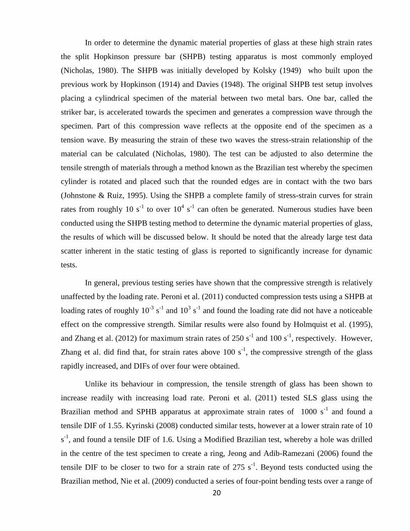
In order to determine the dynamic material properties of glass at these high strain rates

the split Hopkinson pressure bar (SHPB) testing apparatus is most commonly employed

(Nicholas, 1980). The SHPB was initially developed by Kolsky (1949) who built upon the

previous work by Hopkinson (1914) and Davies (1948). The original SHPB test setup involves

placing a cylindrical specimen of the material between two metal bars. One bar, called the

striker bar, is accelerated towards the specimen and generates a compression wave through the

specimen. Part of this compression wave reflects at the opposite end of the specimen as a

tension wave. By measuring the strain of these two waves the stress-strain relationship of the

material can be calculated (Nicholas, 1980). The test can be adjusted to also determine the

tensile strength of materials through a method known as the Brazilian test whereby the specimen

cylinder is rotated and placed such that the rounded edges are in contact with the two bars

(Johnstone & Ruiz, 1995). Using the SHPB a complete family of stress-strain curves for strain

rates from roughly 10 s-1

to over 104 s

-1 can often be generated. Numerous studies have been

conducted using the SHPB testing method to determine the dynamic material properties of glass,

the results of which will be discussed below. It should be noted that the already large test data

scatter inherent in the static testing of glass is reported to significantly increase for dynamic

tests.

In general, previous testing series have shown that the compressive strength is relatively

unaffected by the loading rate. Peroni et al. (2011) conducted compression tests using a SHPB at

loading rates of roughly 10-3

s-1

and 103 s

-1 and found the loading rate did not have a noticeable

effect on the compressive strength. Similar results were also found by Holmquist et al. (1995),

and Zhang et al. (2012) for maximum strain rates of 250 s-1

and 100 s-1

, respectively. However,

Zhang et al. did find that, for strain rates above 100 s-1

, the compressive strength of the glass

rapidly increased, and DIFs of over four were obtained.

Unlike its behaviour in compression, the tensile strength of glass has been shown to

increase readily with increasing load rate. Peroni et al. (2011) tested SLS glass using the

Brazilian method and SPHB apparatus at approximate strain rates of 1000 s-1

and found a

tensile DIF of 1.55. Kyrinski (2008) conducted similar tests, however at a lower strain rate of 10

s-1

, and found a tensile DIF of 1.6. Using a Modified Brazilian test, whereby a hole was drilled

in the centre of the test specimen to create a ring, Jeong and Adib-Ramezani (2006) found the

tensile DIF to be closer to two for a strain rate of 275 s-1

. Beyond tests conducted using the

Brazilian method, Nie et al. (2009) conducted a series of four-point bending tests over a range of

21

strain rates. Their results indicated that the tensile strength of glass increased at higher strain

rates and that this effect was more pronounced in specimens with fewer or smaller surface flaws.

Finally, Zhang et al. (2012) most recently conducted a series of both static and SHPB tests with

strain rates between 58 s-1

and 696 s-1

. From their results they concluded that the tensile strength

of glass initially increases slowly with increasing strain rate until a strain rate of approximately

350 s-1

, at which point the strength rapidly increases. This bilinear relationship is described

using the formulae as follows (Zhang et al., 2012):

μ = 1.137 + 0.015 log(ε) for 1.0−5 ≤ ε ≤ 350 s−1 (2.7)

μ = −2.911 + 1.608 log(ε) for 350 s−1 ≤ ε (2.8)

2.3 Glass Failure Criteria

2.3.1 Introduction

One of the most difficult aspects in assessing the response of glass under loading is

predicting the failure load. As discussed in previous sections, the failure of glass is governed by

the interaction of surface flaws with applied tensile stresses. Therefore, in order to accurately

predict the tensile strength of a glass element a model must be able to account for the size of the

applied load, duration of the loading, area of the element surface placed in tensile stress, and the

size and orientation of the surface flaws. The various methods and models which have been

developed for this purpose are hence overviewed herein.

2.3.2 Deterministic Method

The oldest failure criterion for glass is the deterministic approach which may be referred

to as the maximum principal stress (MPS) method. Essentially, the method states that if the peak

calculated tensile stress exceeds a certain value then failure occurs. This method has been

favoured in the past as it is easy to implement and use. For a monolithic glass pane, the peak

stress may be determined through plate theory calculations and is based upon the geometry of

the plate and the boundary conditions. However, the ultimate strength can only be determined

through experimental testing of the glass material, which often must be conducted under a range

of environmental conditions and load durations in order to account for the effect that these

parameters have on glass strength. Another difficulty in determining the ultimate strength is the

22

fact that the surface flaws, which govern glass failure, are randomly distributed across the

element surface. Therefore, the location of the critical flaw which causes failure often does not

always correspond with the location of maximum principal tensile stress. Further, even after a

statistical value for the acceptable ultimate strength that will result in a low probability of failure

is determined, a factor of safety is routinely required to ensure the safety of this method for

design (Khorasani, 2004).

Despite its shortcomings, the ease of use allowed by the MPS method has allowed it to

become the basis of several standards including prEN 13474-1 (CEN, 1999). For the case of

prEN 13474-1 a basic limiting strength of 45 MPa for soda lime glass is suggested, which is

then modified based upon usage, loading and environmental facts. Ultimately, this method is

directed more towards easing the design burden of engineers and is less effective for evaluation

or analysis of the behaviour of glass.

2.3.3 Stochastic Methods

2.3.3.1 Flaw Statistics

Given that the failure of glass is dependent upon both the presence of a flaw of sufficient

size and a stress of sufficient magnitude, as well as other environmental and load parameters, it

is not surprising that a set of identical specimens may fail at very different loads. Since no single

calculation or empirical measure can accurately represent the failure of glass, statistical methods

are often the best method for predicting glass failure (Shelby, 2005). The Weibull function,

originally devised by Weibull (1939), is commonly thought to be the best representation for the

failure of brittle materials (Overend et al., 2007). The Weibull function represents the

cumulative probability of failure with:

Pf = 1 − exp [−B] (2.9)

where Pf is the probability of failure and B is a risk function. For glass, B is represented by:

B = kAσm (2.10)

where σ is an applied tensile stress over an area A, and k and m represent the surface flaw

characteristics within that area (Beason & Morgan, 1984). The surface flaw parameters m and k

describe the absolute size and density of flaws and the range of flaw sizes respectively. By using

23

Equation (2.10) as the risk function, Equation (2.9) becomes the probability that the area A

contains at least one flaw of a critical size to cause failure, as determined using the fracture

mechanics approach previously described (Fischer-Cripps & Collins, 1995).

The main difficulty in using the Weibull function is that the parameters m and k can only

be determined through an extensive experimental testing series involving locating the critical

flaw through visual inspection and converting the failure load to an equivalent 60 second

duration in order to obtain a stress-time relationship. An iterative statistical process is then

required to determine m and k from the obtained data (Beason & Morgan, 1984). The results of

several testing studies conducted on glass panes to determine m and k are presented in Table

2.1.

24

Table 2.1: Experimental and design values for surface flaw parameters m and k

As-Received Glass (New) Weathered Glass

Study m k m k

Brown (1972) 7.3 5.1 x 10-57

m-2

Pa-7.3

Beason (1980) 6.0 7.19 x 10-45

m-2

Pa-6

Beason & Morgan (1984) 9.0 1.32 x 10-69

m-2

Pa-9

Norville & Minor (1985)

8.0 2.96 x 10-61

m-2

Pa-8

8.8 2.25 x 10-68

m-2

Pa-8.8

9.7 2.25 x 10-68

m-2

Pa-9.7

9.9 6.97 x 10-77

m-2

Pa-9.9

4.0 2.25 x 10-31

m-2

Pa-4

4.1 2.79 x 10-32

m-2

Pa-4.1

4.3 1.89 x 10-32

m-2

Pa-4.3

4.4 6.93 x 10-34

m-2

Pa-4.4

5.5 7.73 x 10-42

m-2

Pa-5.5

6.0 7.3 x 10-45

m-2

Pa-6

6.0 4.54 x 10-44

m-2

Pa-6

6.3 9.64 x 10-48

m-2

Pa-6.3

ASTM E1300 (2009), CGSB (1989) 7 2.86 x 10-53

m-2

Pa-7

Sedlacek et al. (1995), prEN 13474-1 (1999) 25 2.35 x 10-188

m-2

Pa-25

2.3.3.2 Glass Failure Prediction Model

The Glass Failure Prediction Model (GFPM) was developed in the early 1980s by

Beason and Morgan and predicts the probability of a pane of glass failing by relating the surface

25

flaw parameters m and k of the Weibull function to the magnitude and distribution of tensile

stresses in the plate. The model seeks to account for all pertinent parameters which affect glass

strength including the pane geometry, surface area exposed to tensile stress, and load duration.

Specifically, the load duration is accounted for by converting the actual applied stress and its

duration into an equivalent constant load, acting over some duration, which would have the

same effect on an arbitrary surface flaw. This is accomplished using the formulation (Beason &

Morgan, 1984):

where σ(t) is the original stress function, n is a constant commonly taken as 16 for soda lime

glass (Beason & Morgan, 1984), td is the new equivalent duration (typically taken as 60

seconds), and σtd is the new equivalent stress commonly called the “60-sec equivalent stress”.

Equation (2.11) was derived from work conducted by Brown (1974) which related the applied

stress and the resistance of a surface flaw to failure, while exposed to a tensile stress and water

vapour. The model also accounts for the effect of flaw orientation within the tensile stress field,

as well as the possibility of unequal principal stresses through the introduction of a biaxial stress

correction factor, c, in the risk function.

For the case of a thin glass plate, such as a pane of window glass, the surface tensile

stresses will vary with location, load, and time, and thus the Weibull risk function from

Equation (2.10) can be rewritten as (Beason & Morgan, 1984):

B = k ∫ [c(x, y)σmax(q, x, y)]mdAAREA

(2.12)

where c(x, y) and σmax(q, x, y) are the biaxial stress correction factors and the maximum

equivalent principal stress as a function of the uniformly applied lateral load, q, and the location

on the pane (x,y), respectively. The presented risk function can be calculated using either an

analytical or numerical approach and allows the probability of failure to be evaluated for a given

load so long as the surface flaw parameters are known.

σtd = [∫ σ(t)ndt

td

0

td]

1n

(2.11)

26

A criticism of the GFPM is the requirement to rely upon experimental results in order to

determine the surface flaw parameters m and k, which vary widely, and it is therefore at least in

part an empirical model. Further, some researchers have found that the Weibull distribution is

not always the best statistical distribution to describe the failure of glass (Nurhuda et al., 2010).

Despite these criticisms the GFPM does take into account all major known factors which affect

glass strength including plate geometry, surface area in tension, load duration, environmental

factors and the magnitude of the lateral force. As such it has come to be the basis of both

Canadian and American design standards in the forms of CAN/CGSB-12.20-M89 (CGSB,

1989) and ASTM E1300 (ASTM, 2009).

2.3.3.3 Other Models

The first failure model based upon fracture mechanics was developed by Brown (1974)

in the early 1970s. Similar to what Beason and Morgan would later do, Brown combined

Weibull statistics with the load duration equations developed by Charles (1958) and the effects

of relative humidity derived by Wiederhorn (1967) to develop the “Load Duration Theory” for

predicting glass failure. While the full method for calculating the probability of failure using the

Load Duration Theory is beyond the scope of this work, one key difference to be noted between

the GFPM and the Load Duration Theory is in how the arbitrary lateral load is expressed. In the

GFPM the load is changed to an equivalent 60-sec load and any crack growth that may have

occurred in those 60 seconds is ignored. The Load Duration Theory instead makes use of a very

fast applied load to obtain an equivalent instantaneous stress. This results in the Load Duration

Theory calculating higher stresses and thus significantly higher probabilities of failure as

compared to the GFPM (Fischer-Cripps & Collins, 1995).

Weibull statistics were also employed in a model developed by Moore (1980) for

determining the required thickness of glass plates in solar collection panels. Using finite element

models of panels of various aspect sizes and uniform load intensities, Moore devised

dimensionless parameters to describe the bending stresses acting in a pane of glass. These

parameters were used in conjunction with the actual plate geometry and applied loads of a

specific case, and an assumed pane thickness, to arrive at an applied stress value. An ultimate

stress limit was determined using a series of curves which related the probability of failure to a

dimensionless stress value. These curves were derived from a Weibull analysis of experimental

fracture data of glass panes. The applied stress value was compared to the ultimate stress limit to

27

determine if the previously assumed glass thickness was acceptable. A notable limitation of

Moore’s method is that it is only applicable to simply supported rectangular panes (Moore,

1980).

Another group of models, collectively referred to as the “Crack Growth Models”

(CGMs), also employ Weibull statistics in a similar fashion to the GFPM. This group of models

includes the Crack Growth Model and Modified Crack Growth Model (MCGM) as proposed by

Fischer-Cripps and Collins (1995) and the General Crack Growth Model later developed by

Overend et al. (2007). The crack growth models also employ the Weibull function and the same

surface flaw parameters as the GFPM. However, the CGMs differ from the GFPM in how they

determine the critical flaw size. Rather than calculating the probability that an area of glass

contains a flaw that will fail under an equivalent 60-sec load, as in the GFPM, the various

CGMs apply fracture mechanics to determine the minimum flaw size that will grow to a critical

size within the given load duration and the probability that the surface area in tension contains

such a flaw.

A fourth alternative statistics-based method for predicting if a pane of glass will fail

under a given load is to establish the surface flaw parameters, including the size, shape and

locations, and then run Monte Carlo simulations, varying these parameters, to establish a failure

probability curve. Two such models have been developed, the first by Nurhuda et al. (2010)

and the second by Yankelevsky (2014). Both models generate a random flaw map, defining the

flaw location and size and then calculate the failure load based upon whichever flaw will exceed

the critical stress level first. A main difference between these models is how the number, size

and shape of flaws are modelled. Nurhuda’s model uses a Poisson distribution to determine the

number of flaws, one of four probabilistic distributions to select the flaw size, and assumes a

half penny shape for each flaw. Alternatively, Yankelevsky’s model assumes a constant flaw

density of two flaws/cm2, bases the flaw size on Mott’s law and assumes a general crack shape.

In order to generate a failure probability curve, both models run in the order of 5000 trials.

Interestingly, in contrast to previous studies both authors found their results matched statistical

distributions other than the Weibull distribution best. A potential fault of these models is that

neither one accounts for flaw orientation or the effect of non-uniform principal stresses.

28

2.4 Blast Effects on Glazing

2.4.1 Architectural Glazing

As a general term, glazing refers to the set of components which absorbs and transfers

lateral loads to the primary members of a structure and may include glass panes and framing

systems comprised of window frames, mullions and other connecting elements. The present

research is concerned with the basic case of dry-glazed monolithic glass panes, meaning a single

glass pane contained in a frame using rubber gaskets which provide a near simple support

boundary condition. Beyond monolithic glass panes, glazing also encompasses a variety of other

systems including insulated glazing units, curtain wall systems, and structurally glazed systems

where the glass panes are held in place using structural silicon as opposed to rubber gaskets.

Extensive information on these more advanced glazing systems is available in the literature

(Amstock, 1997).

2.4.2 Response of Glazing to Blast Loads

The failure of glazing elements has two serious repercussions in terms of occupant safety

and structural damage. First, upon failure glass will fracture into numerous pieces of various

size and shape depending upon the type of glass. As an example, annealed glass, the focus of

this research, breaks into hazardous dagger-like fragments which are accelerated by the blast

wave and thrust into the structure’s interior at high speed, resulting in contusions and

lacerations. Secondly, the failure of a building’s glazing allows the blast wave to propagate into

the structure potentially resulting in injuries or casualties due to lung and ear damage or by

violently propelling building occupants into walls or other objects (Hadden, 2005; Norville &

Conrath, 2001). Also, upon entering a structure, the blast wave may cause damage to interior

primary structural elements, potentially compromising the structural integrity of the building.

(Norville & Conrath, 2001).

A final point to note is that the response of glazing panels to blast loads is known to be

influenced by the negative phase of a blast wave. In general, the response of any element is

dependent upon the ratio of the blast wave duration to the element’s natural period (td/T) (Pan &

Watson, 1998). For glass panes, testing has shown that, for various scaled distances, this ratio is

such that they experience significant deflections during the negative phase of the blast load and

may be susceptible to failure during rebound, even if the initial positive pressure was resisted

29

(Krauthammer & Altenberg, 2000). Additionally, the vacuum formed during the negative phase

may suck fragments of a broken pane out of the fenestration and into the nearby area, potentially

causing even further damage or injuries.

Experience has shown that the failure of glazing and the resulting projectiles lead to the

majority, upwards of 70%, of all injuries sustained during a typical blast event (Norville, 1999).

It is because of this great potential for human harm and property damage that the response of

glass to blast loads must be understood.

2.4.3 Blast-Resistant Glazing Design

While the scope for the present research is limited to the behaviour of annealed,

monolithic glass panes it should be noted that several glazing technologies are commonly

employed when designing glazing specifically for blast loads. The most common method of

improving a glazing panel’s performance for blast load conditions is to use laminated panes as

opposed to monolithic panes. Laminated panes consist of two or more plies of monolithic glass

bonded together using an elastomeric interlayer, most commonly polyvinyl butyral (PVB)

(Norville & Conrath, 2001). Upon failure, the majority of glass fragments will remain adhered

to the interlayer, thus minimizing the volume of glass which enters the building. Additionally, if

properly designed the interlayer will not tear under the applied load and thus the blast wave will

not propagate into the enclosed space. If absolutely no glass fragments are permitted to enter the

enclosed space, a thin anti-shatter film may be applied to the surface of the inner glass layer.

Either tempered or heat-strengthened panes may also be used instead of typical annealed glass

as a more resistant option. In addition to strengthening the glazing panels, other technologies

such as bomb blast net curtains may be employed to contain the broken pieces of glass produced

by glazing failure (Claber, 1998). Further information on all of these measures designed to

improve the performance of glazing subjected to blast loads may be found in the literature

(Claber, 1998; Norville & Conrath, 2001; Norville & Conrath, 2006).

2.4.4 Testing of Glazing Subject to Blast Loads

The easiest and most reliable method for assessing the resistance of a glazing system to

blast loads is through experimental testing. Such experiments are conducted either through the

detonation of an explosive charge in what is commonly referred to as an “arena test”, or by

using a system known as a “shock tube”. Arena testing of glazing involves mounting the

30

specimen to be tested in a reaction structure, frequently called a “cubicle” or “target”. An

explosive charge of set weight is then placed at a specific standoff distance away from the

cubicle. Using the scaling law as described in section 2.1.3 the charge size and standoff

distance may be altered to change the intensity of the blast load. The other option, of shock tube

testing, simulates the desired blast wave by a burst of compressed air. Regardless of the testing

method, a range of instrumentation is employed to measure both the pressure-time history of the

blast wave and the displacements of the pane being tested. Additionally, a mat or sheet called a

“witness panel” is often mounted behind the glazing panel to collect any broken glass

fragments. Data from the location or trajectory of any glass projectiles may be used to assess the

hazard rating of the test.

Each of the described testing methods possesses its own unique advantages. Shock tube

tests are less expensive, require less set-up and generally allow for more consistent pressure

waves to be generated. On the other hand arena tests mimic actual blast conditions much more

closely. It should also be mentioned that both shock tube and arena tests share some common

limitations. As previously discussed, the results of glass strength tests typically demonstrate a

large scatter and this issue is the same, if not worse, for blast loading. Additionally, blast waves

themselves are highly variable and it is difficult to achieve repeatable loading conditions.

Therefore, it is necessary for a large number of tests to be conducted with either method in order

to obtain trustworthy results.

In spite of any shortcomings of these test procedures each has been adopted by

government agencies in North America and Europe and incorporated into testing standards for

blast-resistant glazing. The shock tube test procedure is outlined in standards BS EN13123-1

(BSI, 2001) and ISO 16934 (ISO, 2007a), while standards ASTM F1642 (ASTM, 2004), GSA

TS01 (GSA, 2003), ISO 16933 (ISO, 2007b) and BS EN 13123-2 (BSI, 2004) describe arena

tests. Each of these standards lays out the charge size and standoff to be used as well as any

requirements for the specimen being tested, the method of mounting the specimen and any

requirements of the testing cubicle in the case of an arena test. In addition, the standards specify

the required instrumentation for each test and the data that is to be collected. This will generally

be a mix of both quantitative and qualitative values including ambient conditions of the test,

pressure-time histories of the blast waves, distance flown of any glass fragments, and

31

description of the glazing and framing system post-testing. A comparison of these testing

standards has been conducted by Walker et al. (2012).

The ultimate goal of these test methods is to provide a quantitative evaluation of the

ability of the glazing arrangement being tested to resist specific blasts. However, even the most

stringently controlled blast tests on glazing will be highly variable in both the loading pattern

and response of the target, making it very difficult to directly compare test results of the glazing

itself. Therefore, how far fragments of broken glass are projected into a standard-sized test

cubicle, as a result of the blast, is generally used as a benchmark to assess the protective ability

of the glazing. The performance specification laid out by the General Services Administration in

TS01 (GSA, 2003) is the most prevalent standard for assessing this result. Essentially, a

standard cubicle, as shown in Figure 2.7, is divided into various regions, each of which is

assigned a hazard rating as listed in Table 2.2. After testing, the floor of the cubicle and the

witness sheet attached to the rear wall are inspected to determine the maximum hazard rating

achieved by the test, as outlined in the standard. Various other standards including ASTM

F1642 (ASTM, 2004), ISO 16933 (ASTM, 2004), and BS EN 13123-2 (BSI, 2004) all also

specify similar testing procedures and performance criteria which will not be included herein.

Table 2.2: GSA performance criteria for blast-resistant glazing

Performance

Condition

Protection

Level

Hazard

Level Description of Window Glazing Response

1 Safe None Glazing does not break. No visible damage to glazing or frame.

2 Very High None Glazing cracks but is retained by the frame. Dusting or very small

fragments near sill or on floor acceptable.

3a High Very Low Glazing cracks. Fragments enter space and land on floor no

furthur than 3.3 ft. from the window.

3b High Low Glazing cracks. Fragments enter space and land on floor no

furthur than 10 ft. from the window.

4 Medium Medium

Glazing cracks. Fragments enter space and land on floor and

impact a vertical witness panel at a distance of no more than 10

ft. from the window at a height no greater than 2 ft. above the

floor

5 Low High

Glazing cracks. Window system fails catastrophically. Fragments

enter space impacting a vertical witness panel at a distance of no

more than 10 ft. from the window at a height greater than 2 ft.

above the ground

32

Figure 2.7: GSA standard test cubicle (adapted from GSA, 2003)

2.5 Numerical Modelling

2.5.1 Introduction

This section reviews the numerical methods by which the behaviour of glazing subjected

to blast loads may be predicted. The typical behaviour of plates under out-of-plane loading is

discussed, followed by the various procedures that can be employed to predict this behaviour.

The most common methods for modelling plates under blast loads are then presented.

2.5.2 Behaviour of Glazing under Out-of-Plane Load

The response of glass panes to out-of-plane loads is often described using thin-plate

theory, since the thickness of the plate is generally much smaller than its other dimensions.

Traditionally, this thin-plate theory is described using Kirchhoff’s classical theory of thin plates

which makes several key assumptions including that the out-of-plane shear stresses are

negligible and that the middle layer of the plate remains essentially unstrained during bending.

Thus, the only stress components under consideration are the in-plane shear and normal stresses

(Szilard, 2004). As an alternative to Kirchoff’s theory, the Midlin thick-plate theory has been

shown to accurately model thin plates (Zienkiewicz & Taylor, 2005). Midlin plate theory

accounts for traverse shear stresses regardless of size. Additionally, the Kirchoff assumption of

an unstrained mid-plane only holds true for small deflections, up to approximately the plate

thickness. However, experience has shown that glass panes routinely deflect several times their

thickness under sudden load such as a blast wave. At these larger plate deflections the mid-plane

becomes stretched producing significant membrane forces which add considerably to the plate’s

33

load resistance (Ugural, 2009). Research has shown that the large-deflection or “Von Karman”

plate theory, which calculates the membrane stresses and superimposes these with the in-plane

bending stresses, may be used in this circumstance to calculate accurate plate stresses and

deflections (Vallabhan et al. 1990). Further, these membrane forces will cause the force-

displacement relationship of the plate to become non-linear due to “geometric nonlinearities”.

Therefore, a geometrically non-linear solution is generally required to accurately describe glass

pane behaviour.

Several methods for solving the differential equations for plate deflections and stresses

involved with the discussed theories are available in the literature. For certain cases of specific

boundary and loading conditions, such as a rectangular, simply-supported plate subject to a

uniform load, closed-form solutions for the plate deflections and stresses may be obtained

(Szilard, 2004; Timoshenko & Woinowsky-Krieger, 1959). However, typically an iterative

process is required to directly solve the differential equations. In order to reduce the

computation effort required with an iterative process, more often one of several numerical

methods is employed.

2.5.3 Numerical Modelling of Plates Subject to Blast Loads

In order to predict the behaviour of glass panes subject to a blast load the equations for

plate deflections and stresses, as mentioned in the previous section, must be solved. Due to the

transient nature of blast loads, a dynamic analysis which takes into account the time variable

must be performed. For modern applications the single degree-of-freedom (SDOF) method and

the finite element method (FEM) method are by far the most popular options.

2.5.3.1 Single Degree of Freedom (SDOF)

The SDOF method is one of the most common approaches for determining the dynamic

behaviour of a structure. By this method, the structure to be analyzed is restricted to only a

single type of motion and is replaced with a system of springs, masses and dampers. Damping is

routinely ignored in blast analysis, as it has little effect on the first peak displacement (USACE,

2008). Therefore, the case of a glazing pane subject to blast loads could be modelled using the

SDOF method with the equation of motion:

KMmy + KLky = KLF(t) (2.13)

34

where F(t), m, and k are the actual applied force, system mass, and stiffness respectively. KM

and KL are the equivalent mass and load factors, respectively, which may be obtained either

through analytical evaluation of the plate deflection equations or using tabulated values such as

those found in Biggs (1964). Also y and ӱ are the central out-of-plane displacement and

acceleration, respectively. Using the KL factor, a static resistance function may then be

constructed. For blast loading cases, s resistance function is an approximation of a structural

elements response against the dynamic blast load in terms of force versus deflection. If the

system bending stiffness is non-linear it may become necessary to use a static resistance

function obtained from experimental testing. Using either a linear spring value or a resistance

function, the support conditions and frame stiffness are directly accounted for in the model

(Biggs, 1964). Equation (2.13) may be solved for a dynamic load using one of a number of

techniques, the most popular being the constant-velocity method.

When applied to the flexural analysis of plates subject to blast loading the SDOF method

allows the time-history of the pane central displacement to be easily calculated. However, this

method is limited in several respects. A shape function must be known or assumed in order to

obtain a complete displacement profile of the plate. Also, the SDOF method assumes a deflected

plate shape based only upon the first mode of vibration, even though it is known that blast loads

excite higher modes of vibration and thus produce a different stress distribution (Norville et al.,

1998). Finally, it is difficult to model complex support conditions using the SDOF method and

research has shown that this method gives overly large deflection values for complex glazing

systems (Cussen & Van Eepoel, 2008).

Despite its shortcomings, the SDOF method has been frequently employed in prior

research for modelling the response of glass panes to blast loads, such as the model developed

by Krauthammer and Altenberg (2000) when investigating the impact of the negative phase of a

blast load on glass panes. Their SDOF model provided similar results to another analytical

model but the authors concluded that there was need for further refinement. Specifically, there

are two main limitations to the SDOF implementation by Kruathammer and Altenberg. First, the

values used to calculate the equivalent system stiffness have been shown to be highly inaccurate

in a number of cases (Morison, 2006). Unless a non-linear static resistance function is

formulated the membrane stresses which develop at large plate deflections will not be accounted

for, and therefore inaccurate displacements will be obtained. Also, while the gross plate

35

behaviour of the plate may be well-modelled using a SDOF approach, much finer discretization

of the plate area, each with its own stress values, is required in order to obtain accurate failure

probabilities (Beason & Morgan, 1984). A more refined SDOF model was developed by

Wedding (2010) with the intention of characterizing a window’s edge reaction forces during a

blast loading scenario. Wedding’s model is much the same as Kruathammer and Altenberg’s,

however it incorporated a non-linear static resistance function. Wedding concluded from his

predictions, which showed exceptionally close agreement with collected experimental data, that

the SDOF method can accurately predict the gross displacement behaviour of a pane of glass

under blast loading (Wedding, 2010).

In addition to the above research investigations the SDOF method has formed the basis

of several design guides and military manuals dealing with the effects of blast loads on

structures (DoD, 2008). Furthermore, SDOF is employed by several major computer analysis

programs including Single degree of freedom Blast Effects Design Spreadsheet (SBEDS)

(USACE, 2009) and Window Glazing Analysis Response and Design (WINGARD) (ARA,

2010). These software programs are discussed in greater detail in Section 2.6.

2.5.3.2 Finite Element Method (FEM)

One of the main reasons for the popularity of the FEM is the ease by which this method

can be applied. Engineers often find the modelling and discretization process to be intuitive and

easy to visualize, thus further easing its implementation (Szilard, 2004). The FEM also

possesses several advantages over the SDOF method in that it can easily account for complex

support conditions, nonlinear material behaviour, and takes into consideration higher modes of

vibration for dynamic analysis. Therefore is it thought that, especially for more advanced

glazing systems subject to blast loads, the FEM will produce more accurate results compared to

the SDOF method (Cussen & Van Eepoel, 2008). A major criticism of the FEM is that it is often

too involved to be used for routine design work or where many iterations may be required.

Frequently the FEM is applied to a specific problem through the use of a commercial

finite element software package such as ANSYS, ABAQUS or LS-DYNA. These programs will

calculate the deflections and stresses of the modelled object, with the designer being responsible

for specifying all relevant material properties, geometry, discretization, boundary conditions, a

suitable loading function and the failure criterion.

36

Apart from the use of general-purpose finite element programs several FEM software

packages have been developed specifically for the design of glazing. The in-development

Curtain Wall Blast (CWBlast) is specifically intended for the analysis of glazing subject to blast

loads and can determine failure using either the MPS method or the GFPM (Seica et al. 2011).

CWBlast is discussed in depth in section 2.6.4.

2.6 Software Packages for the Design of Glass under Blast Loading

2.6.1 Introduction

Currently, several different software products, which can be used for the analysis of

glass panes subject to blast loads, are available. Major topics of focus in this section are: (i) the

method employed for calculating plate displacements and stresses; (ii) which of the previously

covered criteria is used for predicting if and when a glass pane will fail.

2.6.2 SBEDS

The Single-Degree-of-Freedom Blast Effects Design Spreadsheet, or SBEDS, is an

Excel-based tool developed by Baker Engineering and Risk Consultants for the U.S. Army Corp

of Engineers Protective Design Center (USACE, 2009). The program was designed to be in

accordance with the US Department of Defence’s antiterrorism standards, as described in UFC

4-010-01 “DoD Minimum Antiterrorism Standards for Buildings” and UFC 3-340-01 “Design

and Analysis of Hardened Structures to Conventional Weapons”. However, it is regularly

applied for more general analysis of any structure subject to blast loads as described in UFC 3-

340-02 (Polcyn & Myers, 2010).

As its name implies, the program employs the SDOF methodology for the design of one

of 10 predefined structural components subject to dynamic loading. After selecting a predefined

component the user is able to define all aspects of its geometry and material properties. The

boundary conditions can be set as either fixed or simply supported. The member response type

can also be defined to include membrane action along with the flexural response based upon a

selected support capacity. SBEDS also allows the user to define the percent of critical damping

to be used in the analysis. Finally, the target size and incidence angle may be input in order for

potential clearing and reflection effects to be fully accounted for. The blast load may be input

37

using one of three methods: (i) a file generated from another program may be read into the

spreadsheet; (ii) a blast curve may be defined using up to eight pressure-time pairs; (iii) the

program can calculate positive and negative phase pressure curves based upon an entered charge

weight and standoff distance.

In general, SBEDS uses the SDOF equivalency factors as described in section 2.5.3.1

and as listed in Biggs (1964). However, for two-way spanning members, including plates,

recommendations from Morison (2006) have been adopted (Polcyn & Myers, 2010). Using the

determined load equivalency factor, a static resistance function is composed for each phase of

the component response (up to five segments for each of the initial response and rebound)

(USACE, 2008). The response of the entered component for the described blast load is then

obtained using the constant velocity method (USACE, 2008). Once the analysis is complete,

SBEDS outputs results for the system displacement, velocity and acceleration in both graphical

and tabular format. Information on the system stiffness and resistance histories is also available.

The dynamic reactions at each supporting edge are also reported and can be exported for

analysis of other members.

It must be mentioned that the version of SBEDS (version 4.1) utilized for this research

does not include a glazing analysis option and is therefore limited in its capabilities in this area.

The new program, SBEDS-W has been developed for the purpose of the analysis of glazing to

blast loads; however its distribution is restricted and hence unavailable for use herein. Since

SBEDS does not have a built-in method for predicting the failure of a glass pane, it is incapable

of providing an estimate of the time of pane failure or the corresponding fragment velocities and

the hazard rating of the failure. Instead, in order to analyze window arrangements the prebuilt

metal plate option may be selected and one may assume that glass plate failure would occur the

instant SBEDS predicts that the simulated metal plate would first yield. This process is

essentially equivalent to employing the MPS method for predicting failure. Further calculations

are then required to estimate a hazard rating for the test. Needless to say, SBEDS is incapable of

analysis of more complex glazing systems such as multi-plate systems. Laminated systems may

be modelled, however a custom resistance function would need to be defined by the user. This

method of window analysis was utilized in the research presented herein; a full description of its

implementation is provided in section 6.

38

2.6.3 WINGARD

Window Glazing Analysis Response and Design (WINGARD) (ARA, 2010) is a

software program developed for the express purpose of analyzing windows and other glazing

setups for blast loading. Currently, WINGARD is available for purchase from Applied Research

Associates for commercial use. Similar to SBEDS, WINGARD employs the SDOF method for

dynamic analysis. However, it has incorporated several features that are uniquely beneficial for

the analysis of glazing systems.

A four step process is followed to analyze a glazing system using WINGARD. First, all

of the materials used in the glazing arrangement are defined. WINGARD includes libraries with

common material properties for various types of glass, explosives, and interlayers but user-

specified materials can be added. Next, a custom pressure wave may be input either using

pressure-time pairs, which can be entered manually or from a file, or by defining a triangular

linear-equivalent load calculated from an entered peak positive pressure and duration. In the

third step a glazing setup is defined whereby glass, laminate, film and air gap layers in various

standard thicknesses can be combined to model the cross section of the window design to be

tested. Finally, in the fourth step the dimensions and boundary conditions of the window are

defined to form a window system. Uniquely, WINGARD allows for the bite of the window to be

specified, as well as incorporating an option for structural silicone to be used along any of the

edges. If a load was not previously defined, the user may enter a charge weight, standoff and

angle of incidence and let the program calculate the blast wave either as a linear function or

using the Friedlander equation.

The full analysis process employed by WINGARD is not well documented. However,

Morison (2007) has listed some of the fundamental assumptions of the program. The most

relevant of these assumptions for the current work include WINGARD’s use of: Biggs SDOF

equivalency factors (Biggs, 1964); glass failure prediction by Moore’s method as described in

section 2.3.3.3; and damping being defined based upon a percentage of critical damping with a

default value of 2%.

Since WINGARD was developed specifically for the analysis of windows it outputs all

relevant values for evaluating the performance of a glazing system under blast loading. Included

in WINGARD’s output are graphical representations of the window pane’s central

39

displacement, velocity, and acceleration. The program also calculates the dynamic support

reactions along all edges of the window. Additionally, WINGARD will predict the time of

failure of each layer of a glazing setup and output all corresponding values at this time. Based

upon the time of pane failure, WINGARD will predict the flight path of the glass fragments and

calculate the GSA hazard rating of the explosion. Finally, WINGARD will uniquely determine

if and when a glazing pane may “fall out” of its support, based upon the pane deflection and the

bite of the frame.

2.6.4 CWBLAST

Curtain Wall Blast (CWBlast) is a fast-running explicit finite element program designed

for the analysis of various glazing arrangements subject to blast loading (Seica et al., 2011).

This program was developed at the University of Toronto and aims to provide a user-friendly

interface for the application of the FEM for solving glass pane deflections and stresses (Krynski,

2008). The program is not commercially available, but it has undergone some validation by

comparison with static tests and against the dynamic output of another study with good results

(Seica et al., 2011).

CWBlast allows the user to fully describe the window system to be tested. Both window

geometry and height above the floor are first entered. Then the cross section of the window is

described with allowance for up to two separate glazing plates, separated by an air gap, which

may be comprised of glass and laminate layers. The thickness of each layer as well as the

material properties, including any glass prestress values, may be defined or default values are

provided. CWBlast provides extensive freedom for describing the window support conditions,

allowing the user to select one of the eight options shown in Figure 2.8 for each edge of the

window. Once the window system has been defined a blast load may be entered either by means

of charge weight and standoff or by inputting a peak desired positive pressure and impulse. Both

of these methods result in the creation of an equivalent triangular load for the positive phase.

The negative phase is not calculated. As a third option the blast load may be entered manually

using pressure-time pairs. CWBlast uniquely provides the option to load only part of the

window with the load in order to represent scenarios where there may be a partially blocked line

of sight to the window.

40

Figure 2.8: CWBlast support types

Analysis of the window system for the entered blast load is carried out using the explicit

FEM. The finite elements are formulated using a bilinear Lagrangian shape function in

combination with a 2 x 2 numerical integration. Displacements caused by the transient load are

solved using the Newmark-Beta method while stresses are calculated via Mindlin thick-plate

theory. Damping is not considered in the model as it is assumed to have little effect on the peak

response. The user can choose to determine plate failure using either the MPS method or the

GFPM for which the coefficients m and k may be selected. Post failure of the glass elements

CWBlast will calculate the flight paths of the fragments taking into consideration the presence

of the remaining blast load (Seica et al., 2011).

CWBlast outputs most relevant parameters for the evaluation of the performance of a

window under an applied blast load. The displacement at the centre of each pane is available, in

both tabular and graphical format while the corresponding velocity and acceleration values are

provided in only tabular form. CWBLAST also reports the maximum principal tensile stress at

the centre of each pane as well as the highest tensile stress occurring anywhere on the pane. This

is useful as the tensile stress levels at the pane edges or corners may exceed those in the middle

due to plate bending action. The program will also output the time of glass pane failure and the

corresponding deflection and velocity. CWBlast is also capable of outputting the pressure-time

history of the air gap for multi-plate systems. Finally, CWBlast will provide an estimate for the

GSA hazard rating of the window. The only potentially useful output which is not provided by

CWBlast is the dynamic reaction force at the supports.

41

3 Blast Field Testing

3.1 Introduction

Full-scale blast tests were conducted in order to collect experimental data on the

behaviour of monolithic annealed glass panes subjected to blast loads. Testing was first

conducted in 2012 with another testing series occurring the following year. Each testing series

consisted of several monolithic annealed glass panes being tested using the arena blast testing

procedure outlined in Section 2.4.4. The glass specimens were tested under a range of scaled

distances produced through the detonation of ammonium nitrate fuel oil (ANFO) charges. All

tests were accomplished with the assistance of the Explora Foundation.

3.2 Reaction Structures and Test Specimens

The glass component of the test specimens for both series consisted of a monolithic

annealed glass pane, measuring 1 m x 1 m x 12 mm thick. During the 2012 testing series the

bare glass pane was tested, while during the 2013 series the panes were mounted in aluminium

frames using neoprene gaskets to form a dry-glazed window system. The bite of the aluminium

framing was 25 mm, and the resultant exposed glass area of the window was 894 mm x 894

mm.

Reinforced concrete reaction structures were used to hold the glass test specimens for

both testing series. The reaction structures were concrete boxes of various sizes with a varying

number of openings in one face. These openings were framed with steel HSS and angle sections

to facilitate the mounting of the glass specimens. The edges of the openings were located at least

1 m from the edges of the reaction structure to minimize any clearing effects. During the 2012

testing series, a single reaction structure, called Target 1, which held three specimens as shown

in Figure 3.1, was employed. Target 2 and Target 3, shown in Figure 3.2, were added for the

2013 testing series. The bare panes tested in 2012 were secured within the reaction structure

openings using structural silicon along all four edges of the pane resulting in a near wet-glazed

support condition. The windows tested in 2013 were simply fitted within the reaction structure

openings and held in place loosely and therefore exhibited a simply supported edge condition.

42

Figure 3.1: Target 1

Figure 3.2: Targets 2 and 3

3.3 Testing Methodology

Annealed glass specimens were tested at multiple scaled distances over the course of the

2012 and 2013 testing series. In order to mitigate the scatter inherent in glass testing, and

improve the statistical significance of the results, multiple specimens or tests were conducted for

each standoff distance and charge weight combination. For the 2012 testing series, Target 1 was

used to test six specimens over the course of two firings. In 2012 the glass target was tested in

conjunction with several other targets for each firing. Since a large charge size was employed

for these tests a large standoff was also required to obtain a reasonable blast load. During the

2013 blast arena tests, with the addition of Targets 2 and 3, seven specimens were tested during

each of four firings for a total of 28 additional test results. The 2013 glass tests were conducted

- Pressure Gauge

- Pressure Gauge

Pane 1 Pane 2 Pane 3

Pane 1

Pane 2

Pane 1

Pane 2

43

as a stand-alone testing series and much smaller charge sizes and standoffs were employed,

although the scaled distances of the tests were decreased as well. A complete summary of load

parameters for each firing is presented in Table 3.1.

Table 3.1: Blast arena test setups

Year Test Target Standoff (m) Charge Size

(kg, TNT equivalent) Scaled Distance (m/kg

1/3)

2012 1 1 75 410 10.1

2 1 65 410 8.7

2013

1 - 3 1 20 51.25 5.4

2 & 3 17.35 51.25 4.7

4 1 20 41 5.8

2 & 3 17.35 41 5.0

During both testing series, an extensive array of instrumentation was employed to

capture various parameters of the blast load and of the glass response. For all tests, the exact

load produced on the targets was recorded using reflected pressure gauges, which were mounted

flush with the front face of each reaction structure at the mid-height of the windows, as shown in

Figures 3.1 and 3.3 for Target 1. Two reflected pressure gauges were mounted in Target 1 and

one gauge was mounted in each of Targets 2 and 3 (see Figure 3.2). Further data on the blast

waves was collected using free-field gauges mounted on movable support poles. The out-of-

plane displacement of each specimen was captured through the use of LVDT displacement

gauges, which were attached to the centre of the interior face of each pane. In 2013, electrically

conductive paint was used to paint a simple pattern on each pane as shown in Figure 3.4. The

time of pane failure was determined by monitoring the voltage across this painted circuit, as

upon glass fracture the circuit is broken, resulting in an immediate change in the voltage. All

electronic data was recorded using a Hi-Techniques meDAQ data acquisition system with a

sampling rate of 2000 kHz which started recording in time with the charge detonation and

recorded data for the following 1000 msec. In addition to the computer data collection, during

the 2013 testing series tin foil witness sheets were attached to the interior rear wall of each

target and were used to determine the GSA hazard rating for each pane. Also, three high-speed

Phantom video cameras were employed for each test. These cameras were mounted in cases

attached to the rear of Target 1 and were used to capture the time of pane failure and the glass

fracture pattern. The cameras recorded each test at varying speeds ranging from 16,000 fps to

approximately 23,000 fps.

44

Figure 3.3: Target 1 instrumentation

Figure 3.4: Painted break-circuit

3.4 Data Processing

Due to the high data acquisition rate employed during the field tests, the raw data was

inherently noisy and required some processing prior to presentation and analysis. The

proprietary software DPlot (HydeSoft Computing, 2014) was used for this task. Any processing

was kept to a minimum as much as possible to preserve key features of the original data. In

general the same set of modifications was made to each set of data including: (i) setting the data

45

baseline equal to zero for the time period between the charge detonation and the arrival of the

blast wave at the target; (ii) removing any large, obviously erroneous spikes in the data; (iii)

applying a smoothing function to remove any residual noise. The smoothing window was kept

to a minimum in all cases in order to preserve peak values. A representative plot showing a

pressure-time curve before and after this process is shown in Figure 3.5. DPlot was also

employed to produce several other graphs including integrating the pressure-time curves to

produce the impulse-time history of the blast wave and to transform the displacement-time

curve into an approximation of the centre tensile strain versus time plot. Finally, DPlot was used

to create average pressure-time histories using the multiple reflected pressure readings recorded

for Target 1.

Figure 3.5: Raw vs processed blast arena test data

As stated above, part of processing the displacement-time plots was truncating the data

at the measured time of pane failure. In 2012 the time of pane failure was obtained using the

high-speed camera footage of each specimen. During the 2013 tests the novel method of the

painted break-circuit was introduced into the testing series in order to obtain a reliable method

for determining the time of pane failure if no camera footage was available. The failure times

obtained from the new break-circuit method were validated by comparison with the times

indicated by the high-speed video, for those tests where video data was available. The maximum

discrepancy between the two times of pane failure was found to be 0.136 msec, an acceptably

low value, most likely due to the time required for a crack to propagate from its origin through

46

the nearest painted circuit line. Thus, the time of pane failure, as indicated by the break-circuits,

was used to truncate the displacement-time histories of the 2013 tests. A full comparison

between camera and break-circuit failure times is presented in Table A.1 in Appendix A, while

Table A.2 shows the recorded times of failure for the 2013 panes.

3.5 Blast Waves

In general, good readings were obtained for both the free field and reflected pressure-

time histories of each test. Specifically, good agreement between measured free field pressure-

time histories and predictions made using UFC 3-340-02 values for an equivalent hemispherical

TNT charge (DoD, 2008), as implemented in computer program SBEDS, indicate the

detonations occurred as planned. Table 3.2 presents the peak loading values recorded during

each test and a sample reflected pressure-time history is shown in Figure 3.6. All pressure-time

plots are provided in Appendix A, Figures A.1– A.17.

Table 3.2: Blast wave peak positive reflected pressure and impulse values

Figure 3.6: Reflected pressure and impulse (2013, test 1, Target 1)

Target 2 Target 3 Free Field Target 2 Target 3 Free Field

Year Test RP1 RP2 RP3 RP4 FF1 RP1 RP2 RP3 RP4 FF1

1 25.2 27.0 - - - 202 214 - - -

2 36.0 37.0 - - - 241 256 - - -

1 85.0 91.8 135.5 134.2 54.4 345 332 418 472 208

2 79.7 74.0 87.0 108.2 52.3 294 300 318 395 199

3 80.5 85.2 97.3 99.6 50.2 296 300 341 404 203

4 60.0 63.0 82.1 88.1 36.7 246 194 293 344 161

Target 1 Target 1

2012

2013

Peak Positive Pressure (kPa) Peak Positive Impulse (kPa-ms)

47

Referring to Figure 3.6, it can be seen that the reflected pressure readings are also in

good agreement with the SBEDS predictions. However, as was typical for all of the measured

blast profiles, after initially matching the predicted values closely, the measured reflected

pressure begins to dissipate faster than the predictions, resulting in lower than expected

measured impulse. In Figure 3.6 this deviation occurs at approximately 5 ms after the blast wave

arrival. The sudden drop in over-pressure may be attributable to the sudden venting into the

structure, allowed by the failure of the glass panes, as well as by clearing around the reaction

structure. Regardless, from the point of view of the glass behaviour, this discrepancy is not of

significant concern because it occurs after the time when the pane fails, which typically

occurred between 3 to 4 ms following the arrival of the blast wave.

3.6 Displacement-Time Histories

Of the six panes tested in 2012, only a single pane failed during the first test, and no

panes failed during the second test. The fact that no panes failed after decreasing the scaled

distance of the test speaks to the inherent variability present in glass strength. In terms of

displacement measurements, no data was gathered on pane displacements at time of failure.

However, the LVDTs did capture the oscillations of the panes under the applied blast loads, as

shown in Figure 3.7. The remainder of the displacement-time plots from both testing series are

presented in Figures A.18 – A.25 in Appendix A.

Figure 3.7: Measured pane central displacements (2012, test 2)

48

The collected displacement data from the 2012 tests was used to estimate the natural

period of the glass panes and calculate the approximate damping of the system using the log

decrement method. On average, the system’s natural period was found to be 15.5 ms and the

system damping is estimated to be 1.98% with coefficients of variation of 0.04 and 0.25,

respectively. The data used to calculate the natural frequency and damping are presented in

Table A.3 and Table A.4 of Appendix A, respectively. As a point to note, when calculating the

natural period and damping, displacement values were read starting at the second peak to ensure

the system was undergoing free vibration. Figure 3.8 shows the amplitude bounds calculated for

the second test of Pane 3.

Figure 3.8: Pane central displacement and damping boundary (2012, test 2, Pane 3)

Having significantly increased the intensity of the blast loads for the 2013 tests, it was

not unexpected that all 28 tested windows failed. Using the times of failure, as determined from

the break-circuits, the displacement at the point of fracture could be determined and thus offer

insight into the failure behaviour of the glass. A sample displacement-time plot, with the data

truncated at each pane’s time of failure, is shown in Figure 3.9. The average displacement at

failure was found to be 15.6 mm with a coefficient of variation of 0.19. The measured

displacement at failure of each pane is shown in Table A.5 of Appendix A.

49

Figure 3.9: Measured pane central displacements (2013, test 2, Target 1)

The collected displacement data was used to estimate the strain rate experienced at the

centre of each glass pane during the field tests. By assuming a constant elastic curvature across

the width of the pane, the strain at the centre of the pane was estimated based upon elastic plate

theory. DPlot was then used to differentiate the strain with respect to time to determine the

strain rate history of the test, a typical example of which is shown in Figure 3.10. Using this

method the maximum strain rates developed during the arena blast experimentation were found

to be between 0.4 s-1

and 0.8 s-1

for the 2013 test series, and 0.2 s-1

to 0.3 s-1

during the 2012 test

series. These strain rates are much lower than values in the order of 100 s-1

from “typical” blast

tests (Ngo et al., 2007). However, since there was no intended testing rate this difference is

insignificant for future use of the data.

50

Figure 3.10: Measured strain rates (2013, test 2, Target 1)

3.7 Hazard Ratings

After each firing during the 2013 test series, the tin foil witness sheet on the rear interior

wall of each target was inspected and measurements taken of the most critical fragment impact

locations. Using these measurements the GSA hazard rating of the test was determined. Since

the internal dimensions of each of the targets were different to the standard GSA testing cubicle,

the regions as outlined in TS01were adjusted to an equivalent region for each target. The

estimated hazard rating of each test is presented in Table 3.3 and can be related to Table 2.2 for

interpretation.

Table 3.3: Blast arena test GSA hazard ratings, 2013

Target Pane GSA Hazard Rating

Test 1 Test 2 Test 3 Test 4

1

1 5 5 5 OS/4

2 5 5 5 3B

3 5 5 5 3B

2 1 5 5 5 5

3 1 5 5 5 5

The fourth test of Pane 1, Target 1 was assigned a hazard rating of OS, indicating the

failure of the pane was predominately to the outside (OS) of the reaction structure, in addition to

the calculated hazard rating of 4, based upon visual evidence and the displacement-time history

51

of the pane. As seen in Figure 3.11, the majority of glass fragments for this pane were sucked to

the exterior of the structure.

Figure 3.11: Pane failure to outside of reaction structure

3.8 Limitations and Sources of Error

As can be expected, the targets and instrumentation employed during a high-energy blast

test are placed under a significant amount of stress, therefore, accurate data recording is a

challenge. The LVDT displacement gauges were particularly prone to failure. Over the course

of the 2013 testing series, six of the seven displacement gauges failed at various times resulting

in erroneous readings. Apart from failure of the gauges themselves, on at least one occasion the

LVDT-to-glass attachment failed. However, while these problems with the gauges limited the

data collected, the incorrect readings were easy to identify and exclude from analysis of the

data. A more significant potential error in the displacement readings results from the fact that

any settlement of the pane at its supports, from compression of the neoprene gaskets, was not

measured. Therefore, the measured displacement readings may be slightly exaggerated.

The testing environment itself also proved to be a challenge. In particular, during both

testing series the extreme heat of the test site (typically above 40º C) resulted in the high-speed

cameras failing to operate as expected. Even after various heat-relief measures were employed,

several cameras did not trigger properly during the tests. Other difficulties with the site,

52

including limited interior lighting of the targets and excess dust raised by the blasts, resulted in

reduced video quality.

Apart from the difficulties imposed by the nature of the tests themselves, error in the

analysis may be attributed to violation of any of the assumptions made. In particular, the

calculated strain rates are dependent upon the assumed deformed shape of an arc of constant

curvature across the mid-span of the plate. Further, the strain rates are only calculated for an

estimated tensile strain in line with a single major axis, and not for a potentially larger

maximum principal strain. These issues are thought to be of little consequence, however, as the

strain rates were still well below the 350 s-1

threshold indicated by Zhang et al. (2012), or the 10

s-1

value indicated by others (Krynski, 2008), at which the glass strength would be greatly

influenced by a Dynamic Increase Factor.

The calculated hazard ratings may also contain some error as the adjusted hazard regions

used for each target were calculated from the GSA standard using straight line projections, and

did not take into account the arc in a flying fragment’s flight path, as is done in TS01 (GSA,

2003). Therefore, the presented calculated test hazard ratings may be slightly higher than what

would be indicated if a standard-sized cubicle had been employed. Based upon the test results,

this difference would only potentially affect the hazard ratings estimated for the fourth test, as

for all of the other tests the data indicated the panes exceeded hazard rating 5 by a significant

margin.

3.9 Discussion

The blast arena field tests were deemed successful for the purpose of collecting

experimental data on the behaviour of monolithic annealed glass panes under blast loading.

While the 2012 testing series did not provide data on the failure behaviour of the glass panes,

they did provide insight into other aspects of the glass including the natural frequency and

damping of the test set-up. With the decrease in the test scaled distances, and successful addition

of the break-circuits and witness sheets, the 2013 tests provided valuable information on the

failure of glass panes under blast loads including the displacement at failure, and the resulting

hazard rating for each applied load. While instrumentation failure did somewhat limit the data

collected, enough information was gathered from tests to compare against the output of

predictive models and provide insight into their usefulness.

53

For future tests, it is highly recommended that precautions be taken to ensure the

accurate collection of all intended data. Spare replacement LVDTs should be available in case

of any gauge failures. High-speed video cameras should be properly cooled, lenses cleaned and

tested to ensure that the cameras function as intended. Additionally, if possible, targets should

be sized to conform to the specifications of TS01 or another similar standard to ensure that the

collected hazard ratings are correct.

4 Small-Scale Laboratory Testing Program

4.1 Introduction

In order to determine accurate material properties of the glass material tested during the

full-scale field tests, a series of laboratory tests was conducted. Four-point bending tests were

carried out on small beams cut from larger panes of the same material tested in both the 2012

and 2013 blast testing series. From these tests, values for the tensile strength and the modulus of

elasticity of the glass were determined. Prior to conducting the majority of these tests, the effect

of various edge conditions and glass processing procedures on the material response was

reviewed. A three-point bending test series was also conducted in order to compare the obtained

glass strength with the four-point bending response. All bending tests were conducted in the

University of Toronto Structural Testing Facility. Post-testing, the size of the flaw leading to

failure of each of the test specimens was measured and the flaw size distribution of the glass

determined. Details of the investigation and the results from it are presented below.

4.2 Description of Specimens

Initially, four testing standards for the determination of the rupture modulus of glass, as

listed in section 2.2.7, were reviewed. Due to limiting factors, including the specimen

dimensions required for each test and the size of the available glass panes, ASTM C158-12

(ASTM, 2002) was selected for the research herein. This standard prescribes a four-point

bending test conducted on beam specimens approximately 250 mm x 38 mm in size. Since the

same material as used during the blast tests was tested, the specimens were approximately 12

mm thick. The exact specimen dimensions and cross-sectional properties were determined

before testing.

54

All specimens were cut from larger panes of the same batch of material that was used in

the field tests, using the score-and-break technique. As specified in ASTM C158, specimens

were cut such that none of the original edges of the larger glass pane were used as a longitudinal

edge of a specimen. Additionally, half of all specimens were cut orthogonally to the other half

and specimens for each testing series were taken equally from two different panes. All glass

cutting and processing was conducted by Cascade Crystal in Toronto.

4.2.1 Specimen Edge Processing

During production of the test specimens, it was found that the score-and-break method

sometimes resulted in specimens with irregular cross sections along their length. Therefore,

before conducting the tests to determine the glass material properties a smaller set of tests was

conducted to determine if the specimen geometry could be made more regular without affecting

the strength of the glass. Four specimen types were investigated with various combinations of

grinding, corner chamfering and polishing procedures applied after cutting, as follows: type 1,

no additional processing; type 2, grinding and polishing the longitudinal edges; type 3,

chamfering the longitudinal edges; type 4, grinding, chamfering and polishing the longitudinal

edges. Examples showing the cross section of type 1 and type 4 specimens are shown in Figure

4.1 and Figure 4.2, respectively. Any post-cut processing was completed following a six-step

process whereby progressively finer polishing materials were used. The final finish was

obtained using a cerium oxide polish.

Figure 4.1: Type 1, no additional processing (end

view)

Figure 4.2: Type 2, corners chamfered and edges

polished (end view)

Three specimens of each of the four listed types were produced and tested in four-point

bending following the procedure described in section 4.3. The results from these preliminary

tests are presented in Table B.1 of Appendix B. Two points were noted from these preliminary

test results. First, the average strength of the specimen types which had been processed post-

cutting was lower than the specimens which were not processed. Secondly, the specimens that

55

had their longitudinal edges ground down to make them more uniform, consistently failed due to

flaws which originated on a longitudinal edge. This was opposite to the specimens which did not

have their edges ground, which only failed due to failures originating on the face of the beam

surface. It was concluded that while any post-cutting processes did improve the consistency of

the specimen geometry, they also caused damage to the specimen resulting in reduced strength.

This conclusion was supported by a microscope inspection of the specimens as the surfaces

which had been polished showed clear signs of damage while the untouched glass surface did

not. These findings are consistent with previous work which has shown that various cutting and

finishing processes often result in larger flaws along the longitudinal edges of the specimen as

compared to the flat face. These larger edge flaws then typically govern the failure of the

specimen, resulting in a lower recorded failure stress (Corti et al., 2005). Therefore, in order to

ensure that the modulus of rupture of the in-pane glass material was measured accurately, type 1

specimens, with no additional post-cutting processing applied, were used for the testing series

described below.


As stated, specimens were initially tested in four-point bending with a subsequent testing

series conducted using a three-point bending set-up. Conforming to the requirements of ASTM

C158, a span of 200 mm was used with the loading points 100 mm apart (see Figure 4.4). The

load was applied at midspan for the three-point bending tests. The four-point bending test

apparatus is shown in Figure 4.3. For safety reasons, and to facilitate the collection of the

broken glass fragments, an enclosure was placed around the specimen to contain the glass upon

failure.

Figure 4.3: Four-point bending test apparatus

56

The beam specimens were loaded using a servo hydraulic MTS testing machine. The

tests were displacement controlled and a loading of 0.012 mm/s was employed to achieve the

requisite stress rate of approximately 1.1 MPa/s as listed in ASTM C158. In addition to load

measurements, an LVDT was used to measure the midspan deflection of all specimens. Strain

gauges were attached at midspan on both the compression and tensile faces of approximately

one-third of all specimens. A high-speed camera was used to record each test at rates from 6,000

fps to 18,000 fps. Due to the expected high scatter in the data, a minimum of 40 specimens were

tested in each of testing. Upon completion of the tests, the results were used to determine the

glass tensile strength and the elastic modulus of the material, which was calculated from both

the collected strain and mid-span deflection data. The results were also evaluated using a

Weibull distribution which, as mentioned before, is a common statistical method of representing

glass failure strengths.

Following the failure of each specimen, the glass fragments were collected and re-

assembled such that the location of the origin of fracture could be determined. The fracture

origin location was identified both in terms of its position along the length of the beam and

whether it was located along a longitudinal edge of the beam, called an “edge failure”, or on the

surface of the glass called a “face failure”. The failure type was determined by inspection of the

specimen’s failure cross section to identify the location of the pattern described in section

2.2.5.1. Figure 4.4 shows diagrammatically the loading arrangement on a beam and typical face

and edge failure surfaces are shown in Figures 4.5 and 4.6, respectively. Strength results of

specimens which failed from an edge flaw were excluded from calculations of the glass

strength.

Figure 4.4: Loading arrangement for glass beam tests

57

Figure 4.5: Section A-A, typical face failure

Figure 4.6: Section A-A, typical edge failure

Using a microscope, the area surrounding the critical flaw on each specimen was

examined and photographs taken, an example of which is shown in Figure 4.7. From these

images, the mirror radius of each critical flaw was measured. Using the relationships described

in 2.2.5.1, these measurements were used to approximate the flaw length and establish a flaw

size profile for the glass.

Figure 4.7: Close-up of face failure critical flaw origin

4.4 Four-Point Bending Tests

A total of 110 specimens were tested in four-point bending of which 46 were cut from

the same glass used during the 2012 blast arena tests and 64 were cut from panes of the 2013

field test glass. Further, this total includes 89 type 1 (just cut from larger pane) specimens and

21 specimens which received some level of post-cutting processing as described above. Only

specimens which received no additional processing, and failed from a face failure, were used in

58

calculating the glass strength. All test results were used to calculate the elastic modulus of the

material. In relation to this, 28 of the 2012 glass specimens failed from face flaws while the

remainder failed due to flaws originating from a longitudinal edge. Similarly, of the 43 type 1

2013 glass specimens tested in four-point bending, 30 resulted in face failures.

Analysis of the results yielded the material properties shown in Table 4.1 and Table 4.2

for the 2012 and 2013 glass, respectively. The maximum stress was calculated using elastic

beam principles. The elastic modulus (Young’s modulus) was calculated using both the

measured mid-span deflection and mid-span strain data, applying appropriate elastic beam

principles as appropriate. However, only the value calculated from the strain data is shown as it

was decided that the values obtained from the strain measurements were more accurate. This

decision was based upon the variability in the beam cross section along its length, which would

influence its overall deflection behaviour, plus the potential for settlement of the supports

(which was not recorded) which would also affect the deflection readings. Full test results may

be found in Table B.3 and Table B.4 of Appendix B.

Table 4.1: Four-point bending test results, 2012 glass

Failure Load (kN) Tensile Strength (MPa) Elastic Modulus (MPa)

Mean 3.10 85.1 74,600

Median 3.01 82.2 74,900

Standard Deviation 0.654 18.5 3,200

CoV 0.211 0.217 0.043

Table 4.2: Four-point bending test results, 2013 glass

Failure Load (kN) Tensile Strength (MPa) Elastic Modulus (MPa)

Mean 2.99 80.3 75,300

Median 2.96 80.7 75,400

Standard Deviation 0.494 13 2,410

CoV 0.165 0.162 0.032

The reported tensile strength of annealed SLS glass varies in the literature but is

generally less than 100 MPa (Overend & Zammit, 2012) with typical values reported between

40 – 80 MPa. The obtained strengths of 85.1 MPa and 80.3 MPa for the 2012 and 2013 glass,

respectively, are close to this range. The somewhat higher strength values could be due to the

effects of small specimen size. The measured elastic moduli of 74,600 MPa and 75,300 MPa are

very close to the value listed by Menčík (1992) of 74,000 MPa. Therefore, it is thought that the

material properties obtained from the four-point bending test are valid.

59

In addition to the total testing series averages, the average strength value for each group

of specimens cut from a single large pane and sharing a cut direction were also calculated, the

results of which are shown in Table B.2 of Appendix B. As has been mentioned, the surface of a

pane of glass can become damaged in a variety of ways, resulting in lower strength. Even the act

of rolling the glass during production can potentially result in directional flaws and

corresponding lower strength in one direction. Reviewing the average strengths for the group of

specimens that was taken from each pane and orthogonal cut direction, no particular trend could

be determined.

A characteristic trait of glass is the large scatter in data obtained from tests conducted on

seemingly identical specimens under the same conditions. As stated in section 2.3.3 this scatter

is most often described using the two-parameter Weibull distribution listed here as it is applied

to glass panes (Beason, 1980):

Pf = 1 − exp [Akσm] (4.1)

where the m and k are the governing parameters. The latter represents the normalized strength

and m is known as the “Weibull modulus”. Low values of m represent a high level of scatter in

the data while higher values indicate more consistency. Rank regression of the density function

may be employed to determine the Weibull modulus using (Jeong & Adib-Ramezani, 2006):

ln [ln (1

1 − Pr)] = m ln σ + m ln (

1

m)

(4.2)

where:

Pr =i

n + 1

(4.3)

where i is the rank of the specimen from lowest to highest and n is the total number of strength

results. Plotting the left-hand side of Equation (2.9) against its right-hand side, m can be

determined as the slope of the resulting line, where σ, i and n are known. These plots for the

four-point bending strength results are shown in Figure 4.8 and Figure 4.9. For clarity, the m

value obtained from equation 4.2 is not equivalent to the values presented in Table 2.1 for use

with the GFPM, which were obtained using a different statistical analysis method.

60

By the described process a Weibull modulus, m, of 5.28 was obtained for the 2012 glass

while an m of 6.92 was found for the 2013 glass. These values are similar to the reported value

of 5 for glass (Jeong & Adib-Ramezani, 2006). Therefore, the static strength results are also

considered valid in terms of their demonstrated level of scatter.

Figure 4.8: Rank regression of four-point bending strength data, 2012 glass

Figure 4.9: Rank regression of four-point bending strength data, 2013 glass

61

4.5 Three-Point Bending Tests

Fifty six type 1 specimens of the 2013 field blast testing glass were tested in three-point

bending. Forty one of the specimens failed due to a face flaw. Since the sole purpose of these

tests was to determine if the change in testing method would affect the calculated average

tensile strength of the material, only this material property was determined from the results, as

shown in Table 4.3. The full test results are provided in Table B.5 of Appendix B.

Table 4.3: Three-point bending test results

Failure Load (kN) Tensile Strength (MPa)

Mean 1.73 80.9

Median 1.75 82.0

Standard Deviation 0.41 20.1

CoV 0.237 0.249

Generally, four-point bending or ring-on-ring tests are chosen for the testing of glass as

they expose a large portion of the tested specimen to a uniform tensile stress (Shelby, 2005). It

was hypothesized that the average tensile failure stress obtained from three-point bending tests

might be a little higher than from the four-point bending test series. This is because the non-

uniform moment applied in a three-point bending test may cause a specimen to fail not due to

the most critical flaw present, but from a less severe flaw located in a zone of higher applied

stress. The average tensile strength of 80.9 MPa obtained from the three-point bending tests is

only slightly higher than the average value obtained from the four-point bending test series, of

80.3 MPa, for the same glass. This result indicates that, for at least this size of specimen, and the

number of specimens examined, the loading method has little effect on the measured failure

stress of the specimen.

4.6 Flaw Sizes

Post-testing, the fracture surface of each of the beam specimens was inspected under a

microscope to locate the origin of fracture. From this inspection, a total of 89 mirror radii were

located and measured (see Figure 2.6). The half-length (b) of each critical flaw was estimated as

one tenth the mirror radius, as described in section 2.2.5.1. The flaw size distribution is shown

in Figure 4.10. The average flaw length (2b) was found to be 0.153 mm with a standard

deviation of 0.077 mm and CoV of 0.506. Table B.6 in Appendix B presents all data relating to

the measured mirror radii and flaw sizes.

62

Figure 4.10: Critical flaw size distribution

The measured mirror radii were also used to calculate the constant A, as described in

Equation 2.5. After computing A for each test, an average value of 2.05 MPa-m1/2

was found for

this constant. The calculated standard deviation was 0.128 MPa-m1/2

giving a very low CoV of

0.062.

The majority of measured critical flaw lengths ranged between 0.1 mm and 0.3 mm. This

result matches well with previous investigations and with the notion that glass is manufactured

to contain no flaws typically larger than around 0.3 mm (Yankelevsky, 2014). Further, the value

calculated for A of 2.05 MPa-m1/2

is very close to previously reported values of 1.92 MPa-m1/2

(Mecholsky et al., 1974) and 1.82 MPa-m1/2

(Marshall et al., 1980).


As discussed, the score-and-break technique of cutting glass may result in specimens

with non-uniform cross-sectional geometry along their length. Additionally, any specimen

dimensions prior to testing must be limited to the end sections of the beam where it will not be

stressed during testing, as the use of metal measuring tools can damage the glass. Thus, it is

quite challenging to determine the precise geometry at the location of fracture for an individual

specimen. For the presented research, the geometry at each end of the beam specimens was

determined from high resolution scans of the cross section. The dimensions at the location of

fracture were then estimated by interpolating the values at either end of the beam to the point of

63

failure. While it is believed this process provided very close values to the actual dimensions at

the location of fracture, they may not be exact and hence the calculated material properties may

also be slightly in error.

Another factor that may have affected the measured glass strength is any residual stress

present in the glass. Prior to testing, several specimens were examined by a professional using a

polariscope and deemed to be essentially stress free.

4.8 Discussion

Values for both the modulus of rupture and elastic modulus of the glass used during both

of the field test series were successfully determined from four-point bending tests. These

experimentally determined material properties will be used to model the arena tests in each of

the software programs that are to be examined in section 6. The measured glass strengths also

conformed to a Weibull distribution very well, as seen by the R2 values shown in Figure 4.7 and

Figure 4.8 of 0.950 and 0.977, respectively. This close agreement indicates that the Weibull

distribution is appropriate for glass strength results and suggests that models which are based

upon this distribution, such as the GFPM, have a sound statistical basis. Additionally, the

investigation of the fracture patterns yielded a fairly well-populated critical flaw size

distribution. This distribution may prove useful for future modelling endeavours. In particular,

any models which rely on Monte Carlo simulations to predict glass failure may improve the

accuracy of their flaw size distributions based upon the collected data.

Based upon the number of specimens which failed due to edge flaws, it is recommended

for future tests that a minimum of 50 specimens be prepared and tested. (For the 2013 glass, 30

valid “face failures” were obtained from 43 specimens). This will ensure that an adequate

number of face failures are obtained in order to reduce the effect of data scatter when calculating

the tensile strength of the glass.

5 Large-Scale Laboratory Testing Program

5.1 Introduction

Two window systems, identical to the specimens tested during the 2013 field tests, were

tested to failure using a uniformly applied pressure. The first window was tested under static

64

load conditions while the second pane was tested dynamically. The response of the window

systems was used to develop resistance functions for the system as well as to investigate the

boundary conditions provided by the dry-glazed supports. Further, the two tests offered some

insight into the effect of specimen size on glass strength, by comparison with the small-scale test

results. The change in response between the static and dynamic tests was also reviewed. Prior to

testing the second window to failure, the natural frequency and damping of the system were

measured by striking the pane and measuring the resulting out-of-plane vibrations. All testing

was carried out in the University of Toronto Structural Testing Facility. Specifics of the testing

procedure and results are presented herein.

5.2 Description of Specimens

As stated, the window test specimens were identical to those tested during the 2013 field

blast tests. To re-iterate, each window consisted of a 1 m x 1 m x 12 mm thick monolithic

annealed glass pane, dry-glazed in an aluminium frame using neoprene rubber gaskets. The

frame had a bite of roughly 25 mm and the resulting exposed surface area of the glass pane

measured 894 mm x 894 mm.


As discussed in section 2.2.7, the usual method for testing glass panes under a uniformly

applied load is to construct an air-tight box, incorporating the pane as one side and then to

evacuate the air from within the box, using vacuum pressure to apply load. The chosen testing

method herein was to use a water-filled bladder to distribute an applied concentrated load

uniformly over the surface of the glass. For this purpose a custom bladder, made of PVC coated

28 oz. polyester fabric, of approximate size 894 mm x 894 mm x 150 mm, was ordered from

SEI Industries. A cross-sectional view of the test setup is shown in Figure 5.1. As shown, the

pane to be tested was supported horizontally on top of an HSS frame (which was supported on

three load cells). The bladder was placed on top of the glass and confined on its four vertical

sides by a square wall constructed from channel segments which sat on the window’s aluminium

frame. A steel plate, sized to snugly fit within the channel section wall, was attached to an MTS

machine via an HSS extension. By lowering and subsequently pushing on this plate, pressure

was exerted on the bladder which then exerted an equal, uniformly distributed, out-of-plane

pressure over the entire exposed glass area of the window. Figure 5.2 shows this apparatus setup

65

for the second test. Plastic sheeting and wooden walls were erected surrounding the apparatus as

a safety precaution.

Figure 5.1: Full-scale testing apparatus cross section

Figure 5.2: Full-scale testing apparatus, test 2

A question raised by the chosen testing method was whether the bladder, once filled,

would conform to the surface of the glass uniformly, particularly near the edges of the pane.

Visual inspection of the filled bladder from the opposite side of the glass pane showed that, in

general, the bladder conformed to the glass surface very well, as seen in Figure 5.3.

66

Figure 5.3: Bladder conforming to glass surface, pretesting trial

During each test, the applied load, pane displacement and planar strains were recorded.

The HSS base frame of the testing apparatus rested on three load cell “legs”. The magnitude of

the uniformly distributed load was determined by summing the load cell forces and dividing it

by the area of the pane. Five displacement gauges were used to determine the displacement of

the glass pane. One gauge was placed at the centre of the pane and one was placed at midspan,

along each edge of the pane (see Figure 5.4) to measure the displacement caused by settlement

of the neoprene gaskets and the test frame. Finally, a total of 46 linear strain gauges were

adhered to each pane to measure strains at various locations. Three gauges were placed to form

strain rosettes in each corner and at the centre of the pane. Additionally, two strain gauges were

placed at midspan of each of the pane edges, one parallel to the edge and the second placed

perpendicular to it. At all locations, gauges were adhered to both the tensile and compressive

faces of the pane, opposite each other. Referring to Figure 5.4, thin neoprene strips were used to

separate the aluminium frame from the confinement wall, preventing the strain gauge wires

from being pinched at this location.

67

Figure 5.4: Displacement gauge locations for full-scale laboratory tests

Each test followed a specific loading sequence. First, the window system and channel

section confinement wall were positioned and stacked according to Figure 5.1. At this point the

load cells were zeroed, and thus all loading resulting from the bladder was subsequently

measured. Next, the bladder was positioned within the confinement wall and filled with water.

Once the bladder was filled the loading plate was lowered, and the bladder compressed slightly

while its valve remained open allowing any residual air to be expelled. From this point on the

two panes were tested at different loading rates. For the first test a quasi-static loading case was

desired. To achieve this, the loading plate was lowered at a rate of 0.075 mm/s. A dynamic

loading rate was achieved for the second test by lowering the plate at an approximate rate of 60

mm/s. As stated, prior to testing the second window, the natural frequency and damping of the

system was investigated by striking the glass pane with a rubber mallet to excite the system. The

resulting pane oscillations were recorded using the centre displacement gauge.

5.4 Large-Scale Laboratory Test Results

To determine the natural frequency and damping of the dry-glazed window system, the

second of the two tested panes was excited a total of 26 times, and the resulting vibrations

measured, prior to its testing to failure. From these tests the average natural period was found to

- Displacement Gauge

68

be 21.8 ms with a standard deviation of 0.78 ms and a corresponding CoV of 0.036. The average

damping of the system was found using the log decrement method, and was calculated as 4.09%

with a standard deviation and CoV of 0.81% and 0.197, respectively. Both of these values are

higher than those obtained for the wet-glazed test setup used during the 2012 field tests, for

which a natural period of 15.5 ms and a system damping of 1.98% were found. The data used to

calculate the natural frequency and damping is provided in Table C.1 and Table C.2 of

Appendix C. A sample graph showing the pane oscillations as well as the calculated damping

boundary is shown in Figure 5.5.

Figure 5.5: Pane central displacement and damping boundary (test 3)

The first window, which was tested statically, failed at a total applied load of 24.4 kN,

equivalent to a uniformly applied load of 30.5 kPa. By visual inspection of the shattered pane,

the fracture origin was located at co-ordinates of (340, 265) mm from the pane corner. Using the

method previously discussed in section 4.6, the critical flaw length was measured as 0.386 mm

long. By substituting the previously calculated value of 2.05 MPa-m1/2

for A in equation 2.5, the

failure stress for this test was found to be approximately 46.7 MPa. It is understandable that this

failure value is significantly lower than the average tensile strength obtained from the small-

scale bending tests of 80.3 MPa, as a much larger area of glass was exposed to a tensile stress

field for the full-scale pane test. As expected, the second test, which was tested at a much faster

rate, failed at the much higher load of 56.2 kN, equivalent to a uniform pressure of 70.3 kPa. For

this test the critical flaw was located at (587, 329) mm and was found to be approximately 0.100

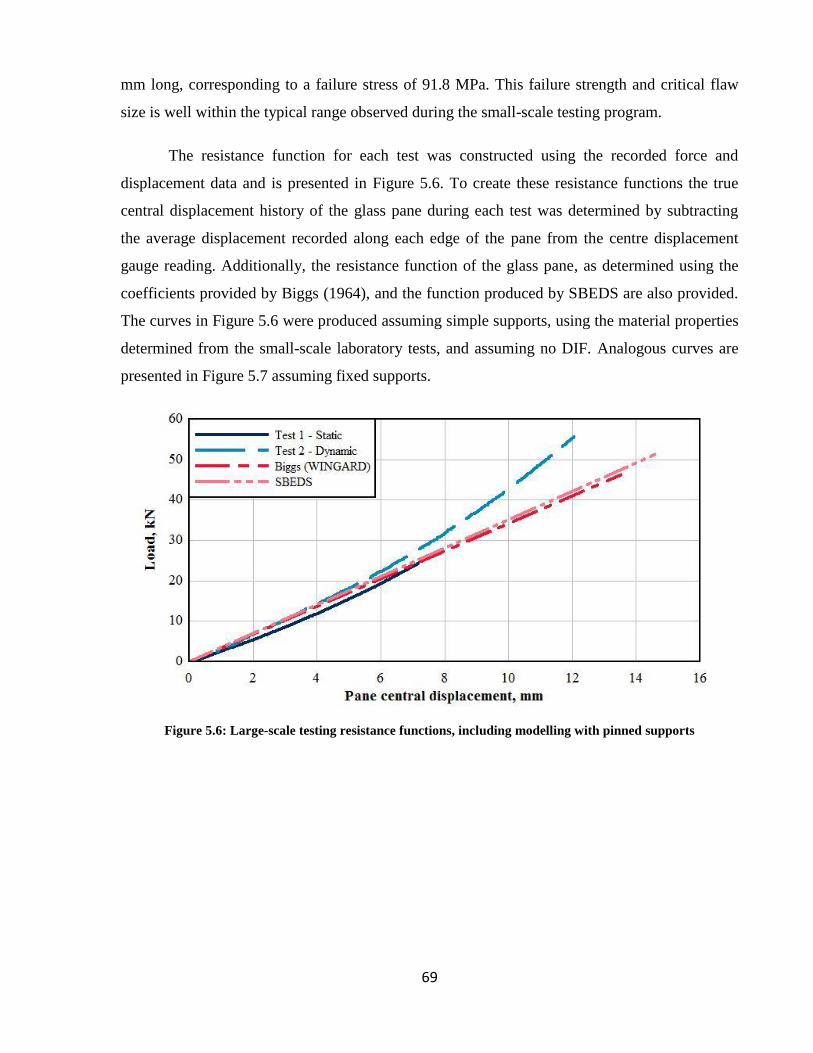
69

mm long, corresponding to a failure stress of 91.8 MPa. This failure strength and critical flaw

size is well within the typical range observed during the small-scale testing program.

The resistance function for each test was constructed using the recorded force and

displacement data and is presented in Figure 5.6. To create these resistance functions the true

central displacement history of the glass pane during each test was determined by subtracting

the average displacement recorded along each edge of the pane from the centre displacement

gauge reading. Additionally, the resistance function of the glass pane, as determined using the

coefficients provided by Biggs (1964), and the function produced by SBEDS are also provided.

The curves in Figure 5.6 were produced assuming simple supports, using the material properties

determined from the small-scale laboratory tests, and assuming no DIF. Analogous curves are

presented in Figure 5.7 assuming fixed supports.

Figure 5.6: Large-scale testing resistance functions, including modelling with pinned supports

70

Figure 5.7: Large-scale testing resistance functions, including modelling with fixed supports

Comparing Figures 5.6 and 5.7, it is shown that the experimentally obtained resistance

functions match the curves calculated assuming simple supports much more closely than the

curves assuming fixed supports, suggesting that the rubber gasket supports of the aluminium

frames offer little rotational resistance. Beyond a visual comparison of the resistance function

curves, calculated values for the Young’s Modulus of the glass panes also support the

conclusion that the aluminium frames mostly closely behave as simple supports. Assuming

simple support conditions, Navier’s method (Timoshenko & Woinowsky-Krieger, 1959) for

calculating plate deflections was employed to determine the Young’s Modulus of the glass

material during the linear period of each experimental resistance function (taken as displacement

less than 4 mm). Similarly, Lévy’s method (Timoshenko & Woinowsky-Krieger, 1959) was

used to determine the glass elastic modulus assuming fixed supports. For the simply supported

case, Young’s Moduli of 63,700 MPa and 75,900 MPa were calculated from statically and

dynamically determined resistance functions, respectively. Assuming fixed supports an E for the

glass of 19,800 MPa was found from the static laboratory test while the dynamic test yielded a

value of 23,500 MPa. Recalling that the Young’s Modulus of the glass was determined to be

75,300 MPa from the small-scale tests (Section 4.4), clearly the assumption of simple supports

results in much more accurate models of the window system.

Focussing on Figure 5.6, the response of the window system during both tests initially

closely follows the predicted responses provided by SBEDS and Biggs. However, the second

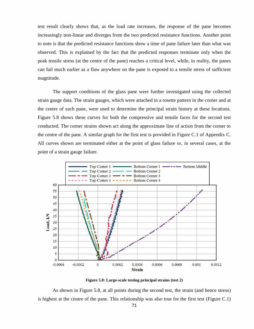
71

test result clearly shows that, as the load rate increases, the response of the pane becomes

increasingly non-linear and diverges from the two predicted resistance functions. Another point

to note is that the predicted resistance functions show a time of pane failure later than what was

observed. This is explained by the fact that the predicted responses terminate only when the

peak tensile stress (at the centre of the pane) reaches a critical level, while, in reality, the panes

can fail much earlier as a flaw anywhere on the pane is exposed to a tensile stress of sufficient

magnitude.

The support conditions of the glass pane were further investigated using the collected

strain gauge data. The strain gauges, which were attached in a rosette pattern in the corner and at

the centre of each pane, were used to determine the principal strain history at these locations.

Figure 5.8 shows these curves for both the compressive and tensile faces for the second test

conducted. The corner strains shown act along the approximate line of action from the corner to

the centre of the pane. A similar graph for the first test is provided in Figure C.1 of Appendix C.

All curves shown are terminated either at the point of glass failure or, in several cases, at the

point of a strain gauge failure.

Figure 5.8: Large-scale testing principal strains (test 2)

As shown in Figure 5.8, at all points during the second test, the strain (and hence stress)

is highest at the centre of the pane. This relationship was also true for the first test (Figure C.1)

72

and is indicative that the pane boundaries are closer to simple supports, as opposed to fixed. The

strain readings from gauges above and below each other at the pane corners, where the tensile

and compressive strains are approximately equal, are also significant (Figure 5.8). The corner

strain readings indicate tensile strain in the top surface of the pane and compression in the

bottom face, which would be the case for a plate simply supported along all four edges

(Timoshenko & Woinowsky-Krieger, 1959).

Further analysis of the collected strain data supports the conclusion that the window

frames act in mostly a pinned fashion. Table 5.1 presents a comparison of measured pane central

strains at the peak load of each test with the strains predicted for the same location calculated by

plate theory, assuming either simple or fixed edge conditions. For the static test, the simple-

support predictions are almost identical to the measured strains from the tests. For the dynamic

test the bottom face readings fall between the two predicted values while the top face readings

match best with the fixed-support model. However, it is felt that the top face strain gauge for the

second test may have been in error as it does not align well with the other collected data.

Additionally, since the strains on the top and bottom faces at the centre of the pane are of

roughly the same absolute magnitude for the first test, it appears that no significant tensile

membrane action formed due to lateral restraint at the supports. A similar comparison of

measured versus predicted strains is presented in Table 5.2 for the collected bottom face strains

at the middle of each edge. For this location the simple-support predictions match the measured

values much more closely than the fixed-support case, for both the static and dynamic tests.

Overall, the measured strain data provides strong evidence that the windows are best modelled

with simple-support edge conditions. Plots of the measured pane central and edge strains are

presented in Figures C.2, C.3, C.4 and C.5.

Table 5.1: Measured and predicted pane central strains

Average Strain (x 10

-6)

Measured Simple Supports Fixed Supports

Test 1 Top Face -581 -607 -312

Bottom Face 591 607 312

Test 2 Top Face -554 -1400 -718

Bottom Face 994 1400 718

73

Table 5.2: Measured and predicted pane edge strains

Average Bottom Face Strain (x 10

-6)

Measured Simple Supports Fixed Supports

Test 1 94 84 -692

Test 2 268 194 -1595

The principal strain at the centre of the pane was also used to calculate the strain rate for

each test. A strain rate of approximately 2.5 x 10-6

s-1

was found for the first test and a strain rate

of 2.45 x 10-3

s-1

was found for the second test. As such, the first test was clearly conducted

within the static regime while the second test may only have reached an intermediate or

quasistatic testing rate. It is therefore unlikely that the strain rate of the second test had a

significant effect on the strength of the glass.


The largest limitation of the large-scale laboratory testing program is the limited number

of specimens tested. As seen during the small-scale testing, the results of glass testing are

inherently highly variable. Since only two specimens were tested, at different loading rates,

limited conclusions may be drawn from the test data. Specifically, it is uncertain whether the

demonstrated failure stresses are typical or outlying values. Also, the limited data prevents any

comparison between the results of the two tests to determine the exact effect of the change in

loading rate on the glass response.

The second major challenge encountered during the large-scale pane testing was failure

of the strain gauges. Despite efforts to minimize the crushing effects, several strain gauges

adhered to the compression face of the glass failed throughout both tests. The failure of gauges

in these locations is likely due to the wires being crushed underneath the bladder. Most

significantly, all of the gauges attached at the midspan of each edge on the top surface failed

during each test, preventing the measurement of any tensile membrane strains there.

5.6 Discussion

The large-scale laboratory testing provided useful insight into the behaviour of the tested

windows and will assist with future modelling of this system. The experimentally determined

resistance functions are of particular significance. As shown by the experiments, the resistance

74

function of the windows is not a linear function, as is typically employed by software programs,

but has at least a slight degree of non-linearity, especially for higher applied loads. As such, the

accuracy of software predictions may be improved through the use of the experimental

resistance function. Additionally, the result of the first test shows that glass is susceptible to

failure earlier than would be determined using the MPS failure criterion, if a significantly large

flaw is present. Thus, some doubt is cast upon whether a program which relies upon the MPS

method can safely be relied upon to predict glass failure. This topic will be explored further in

section 6.

Beyond the resistance functions, the large-scale tests also clarified the nature of the

support conditions. In general, the resistance functions (Figure 5.6) and strains (Table 5.1 and

Table 5.2) predicted assuming simple supports matched the measured data much closer than if

fixed supports were assumed. Also, estimating the Young’s Modulus of the glass from the

collected data assuming pin supports yielded values much closer to the previously established

value obtained from the small-scale testing than similar estimates using fixed supports.

Ultimately, the aluminium frames and rubber gaskets appear to act as simple supports most

closely and will therefore be modelled as such in section 6.

Finally, the large-scale tests also allowed the natural period and damping of the window

system to be measured. Since all of the windows tested during the 2013 testing series failed

under the applied blast load, these values could not be determined in the same manner as they

were for the wet-glazed panes tested in 2012. In addition to potentially improving some of the

software models, these values can be used for comparison purposes with the software

predictions to evaluate their accuracy.

Future tests of a similar nature could be improved in several ways. It is highly

recommended that a larger number of panes be tested, such that statistically significant averages

for key parameters, such as the failure load, may be determined. Any strain gauges to be placed

on the compressive face should be mounted to minimize the length of wire placed under the

bladder and wires should be run in flat straight lines as much as possible. Finally, it may be

beneficial to apply a lubricant to the inside surfaces of the confinement wall to reduce possible

frictional effects between the bladder and this surface.

75

6 Blast Modelling with Software

6.1 Introduction

This chapter compares the collected experimental data from the 2012 and 2013 blast

arena tests with the output of three computer programs: WINGARD PE (ARA, 2010), SBEDS

(USACE, 2009), and CWBlast (Seica et al., 2011). The glazing systems tested during each of

the field tests were modelled in each of the software packages and the recorded pressure-time

histories were used for the load input. Data gathered from both the small and large-scale

laboratory tests was used to improve the accuracy of the input to the software models. The

precision of the glass pane response predicted by each of the programs is compared against the

collected experimental data based upon several parameters. Of particular interest is the accuracy

of the predicted displacement-time histories, including the calculated times of pane failure, and

the ability of the programs to estimate the hazard level for each of the tests. Based upon the

results of these comparisons the reliability of each computer program and the methods it

employs are evaluated. Further, the applicability of the GFPM for blast loading scenarios is

reviewed.

6.2 Modelling Methodology

A brief overview of each of the software packages employed has been previously

provided in section 2.6. In general, the procedure for modelling the field tests was similar for

each program. In each case, the glazing system was modelled as a simply supported plate, and

the loading was entered using the recorded pressure-time histories of the field tests. Common

features across all of the models include: simple supports for the boundary conditions, the glass

pane dimension, the geometry of each target, and material properties (for which the values

obtained from the small-scale laboratory tests were used). However, the various analysis

methods of the programs, the unique way in which each one predicts pane failure, and each

program’s ability to estimate the GSA hazard ratings, necessitated several key differences in the

use of each software package, which are discussed herein.

6.2.1 SBEDS Modelling

As previously mentioned, SBEDS is not specifically designed for the analysis of glazing.

However, two possibilities are available for the analysis of glass panes using this program. The

76

first option is to model the glazing using SBEDS’s “metal plate” template which will generate a

resistance function based upon the user-entered geometry and material properties. Alternatively,

SBEDS’s general SDOF template can be developed to model a plate similar to the metal plate

template, except the user can enter a more customized resistance function. Ultimately, the

difference between these methods amounts to selecting which resistance function best represents

the glazing being analyzed. Whichever option is selected, the user must determine failure by

assuming the pane fails upon reaching a certain “yield” load, defined as the system reaching the

peak of the defined resistance function. This method for predicting pane failure is equivalent to

employing the MPS failure criterion. Sample input sheets for both methods are shown in Figures

D.1 and D.2 of Appendix D.

Both methods of modelling the tested glass panes in SBEDS were employed. The

resistance functions determined from the large-scale laboratory testing, both static and dynamic,

(see section 5.4) were used with the general SDOF template. Since SBEDS limits the entry of

custom resistance functions to five linear segments, it required that the non-linear resistance

functions obtained from the laboratory tests be converted to a series of linear segments. Further,

a DIF of 1.129 for the 2012 tests and 1.136 for the 2013 tests, as calculated using equation 2.7,

was used with SBEDS’s “metal plate” template, while no DIF was applied to the measured

resistance functions used with the general SDOF template. A sample graph, showing the

displacement-time history predicted using each method for a single test is shown in Figure 6.1.

Each curve has been terminated at the predicted point of pane failure.

77

Figure 6.1: SBEDS-predicted pane central displacements (2013, Target 1, test 1, pane 2)

Two points are clearly shown by Figure 6.1. First, the small differences in pane stiffness

amongst the three employed resistance functions have little effect on the shape of the

displacement curve, as the three predicted curves overlap. Secondly, the choice of resistance

function includes the point of pane failure based on the experimental results of Figure 5.6,

which are likely very dependent on flaws in the glass. The two predictions based upon the

experimentally determined resistance functions (rather than small-scale material properties)

should more accurately reflect the true pane behaviour, as predicted using SBEDS SDOF

implementation. Further, while only two full-sized panes were tested in the laboratory, and

therefore no average resistance function is available, it may be assumed that the average

response of the pane would fall between the results of the two conducted tests. This assumption

is based upon the measured critical flaw size of each of the full-scale tests, 0.386 mm for the

static test and 0.100 mm for the dynamic test, and the average flaw size obtained from the small

scale testing of 0.154 mm, which suggests that the response of the two tests fell on either side of

an assumed average response.

Another previously discussed issue with modelling the response of the glass panes in

SBEDS is the fact that the program cannot predict GSA hazard ratings. As the hazard rating is a

crucial design criterion for glass under blast loading, and hence a key area of comparison

78

between the predictive models and the experimental data, one has to resort to estimating the test

hazard rating based upon SBEDS’s output. A method to accomplish this is to take the predicted

pane central velocity at the time of failure and increase it based upon the maximum remaining

impulse that may be transferred to the pane from the blast load, to obtain a conservative velocity

for the glass fragments. Using this velocity the flight path of the glass fragments may be

calculated using elementary physics equations and a hazard rating may then be estimated.

6.2.2 WINGARD Modelling

The use of WINGARD to model the experimental tests was a relatively straightforward

process, following the steps outline in section 2.6.2. One unique aspect of the WINGARD

models are the boundary conditions. For the 2012 tests the WINGARD wet-glazing option was

enabled to more accurately model the field conditions. Default values for the silicon strength

and bead size were used. Furthermore, for all tests the glazing bite was specified as 25 mm. The

WINGARD models were also adjusted to incorporate the DIF calculated using equation 2.7

rather than the program’s default values. This amounted to relatively small changes in the

dynamic strength of the glass material properties from 94.3 MPa to 96.1 MPa (DIF of 1.108 to

1.129) for the 2012 glass and from 91.7 MPa to 91.2 MPa (DIF of 1.142 to 1.136) for the 2013

glass. Finally, WINGARD requires the use of predefined thickness when developing glazing

layups, therefore the glass thickness was modelled using the closest available option of 11.9

mm. This thickness does fall within the range of values measured from the small scale beam

specimens which varied in thickness between 11.83 mm and 12.17 mm. Figures D.3 through

D.5 show sample values for key WINGARD parameters.

6.2.3 CWBLAST Modelling

Similar to SBEDS, there are several options for modelling glazing panes in CWBlast in

terms of the failure criterion employed, as both the MPS method and an implementation of the

GFPM model are available. Further, as shown in Table 2.1, there is a great deal of variability in

the values that can be entered for the Weibull parameters m and k. For the presented work, the

field tests were modelled using both failure criteria. Figure 6.2 demonstrates how the pane

response varies depending on which failure criterion is selected, and which values are taken for

the Weibull parameters. Since the panes test in the field were considered to be new glass the

range of Weibull parameters examined was limited to the range of the as-received column of

79

Table 2.1 (excluding Sedlacek et al.). The Weibull parameters given in ASTM E1300 were also

employed. All GFPM models were run until the probability of failure reached 50%, to simulate

the average response. Example CWBlast input is presented in Figures D.6 to D.10 of Appendix

D.

Figure 6.2: CWBlast-predicted pane central displacements (2013, Target 1, test 1, pane 2)

Reviewing Figure 6.2, it is clear that while the failure prediction method and the Weibull

parameters have no impact on the shape of the displacement curve (all plots overlay each other),

they do have a significant influence on CWBlast’s predicted time of pane failure. In general, the

use of the GFPM results in later predicted failure times and hence higher final displacements

compared with the MPS method. Of particular note is the non-uniform way in which the

predicted time of pane failure changes, based upon which m (and corresponding k value) is

employed for use with the GFPM failure criterion. As one would expect, increasing m from 7.0

to 8.0 results in a later time of pane failure. However, for m values of 7.3, 8.8 and 9.9 the

predicted times of pane failure are almost identical, and much later than for an m of 8. Further,

for an m value of 9.7 the pane is predicted to fail shortly after the blast wave’s arrival. With

these results in mind, when comparing the predictions of CWBlast with the experimental data,

the results obtained using m values of 8.0 and 8.8 were used to show the approximate range of

response the GFPM may predict for new glass. In addition the CWBlast predictions obtained

using the Weibull parameters of m = 7 and k = 2.86 x 10-53

m-2

-Pa-7

, as employed by ASTM

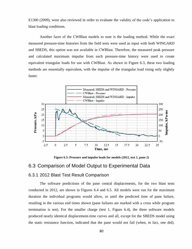
80

E1300 (2009), were also reviewed in order to evaluate the validity of the code’s application to

blast loading conditions.

Another facet of the CWBlast models to note is the loading method. While the exact

measured pressure-time histories from the field tests were used as input with both WINGARD

and SBEDS, this option was not available in CWBlast. Therefore, the measured peak pressure

and calculated maximum impulse from each pressure-time history were used to create

equivalent triangular loads for use with CWBlast. As shown in Figure 6.3, these two loading

methods are essentially equivalent, with the impulse of the triangular load rising only slightly

faster.

Figure 6.3: Pressure and impulse loads for models (2012, test 1, pane 2)

6.3 Comparison of Model Output to Experimental Data

6.3.1 2012 Blast Test Result Comparison

The software predictions of the pane central displacements, for the two blast tests

conducted in 2012, are shown in Figures 6.4 and 6.5. All models were run for the maximum

duration the individual programs would allow, or until the predicted time of pane failure,

resulting in the various end times shown (pane failures are marked with a cross while program

termination is not). For the smaller charge (test 1, Figure 6.4), the three software models

produced nearly identical displacement-time curves and all, except for the SBEDS model using

the static resistance function, indicated that the pane would not fail (when, in fact, one did).

81

Under the larger applied load (test 2, Figure 6.5), three of the models including the static

resistance SBEDS model and two CWBlast models, indicated that the panes would fail at the

time and displacements shown. The majority of the models still show the window to not fail

(and, in fact, no panes failed). The differences between the observed and predicted times of pane

failure are a reflection of the failure criteria in the software versus the cause of failure in the test

panes, the latter being flaw-size dependant.

Figure 6.4: Measured and predicted pane central displacements (2012, test 1)

82

Figure 6.5: Measured and predicted pane central displacements (2012, test 2)

Comparing the model results to the collected experimental data, there are clear

discrepancies in terms of the peak predicted displacements, in both the positive and negative

directions. Also, the model-predicted periods of vibration, as shown in Table 6.1, are all slightly

shorter compared to the field test data. A potential explanation for the period discrepancies is

that, despite best efforts to be accurate, the software models are still stiffer than the actual

glazing set up.

Table 6.1: 2012 Measured and predicted periods of vibration

Period of Vibration (ms)

Measured CWBlast SBEDS WINGARD

Test 1 Test 2

Pane 1 - 14.7

13.7 13.4 13.8 Pane 2 14.7 15.6

Pane 3 14.2 15.0

6.3.2 2013 Blast Test Result Comparison

During the 2013 blast tests, the recorded pane behaviour, including displacement at

failure and failure times, varied between each test and amongst the three targets. However, the

83

trends observed when comparing the recorded displacement-time histories with the model

predictions are well-represented by the sample plots shown in Figures 6.6 and 6.7. Again, the

point of pane failure, either as measured or predicted, is marked with a cross for each line.

Additional plots from the 2013 tests are shown in Figures D.1 to D.2 of Appendix D.

For the first three tests, when a larger charge size was used, all of the models indicated

pane failure. As can be seen though (Figure 6.6), there are significant differences between the

models and the experimental data in terms of the predicted time of pane failure and the peak

central displacement. In general, the “metal plate” resistance function SBEDS model and the

GFPM employing an m value of 8.8 over-predicted the time and final displacement of the panes.

On the other hand the static resistance function SBEDS model and CWBlast MPS model both

predicted pane failure much earlier than observed during the field tests. The other four models

all produced fairly close results in terms of the average displacement at failure, although they

generally also predicted failure sooner than recorded. For a few cases the pane displacements

were most closely in line with the higher displacement predictions made by the “metal plate”

SBEDS model and the m = 8.8 GFPM model. However, these recordings may have been a result

of stronger than average glass panes.

Only a single displacement record was obtained from the fourth test in 2013 (Figure 6.7).

This displacement-history is from the pane which ultimately failed to the exterior of the reaction

structure, discussed in section 3.7. Comparing it to the model predictions one can see that the

software packages greatly under-predict the maximum displacement of the pane. Other points to

note are that the SBEDS model using the “metal plate” template predicted that the pane would

not fail at all, and that the GFPM employing an m of 8.8 was the only model to predict pane

post-peak displacement.

84

Figure 6.6: Measured and predicted pane central displacements (2013, test 2, Target 1)

Figure 6.7: Measured and predicted pane central displacements (2013, test 4, Target 1)

85

Another area of comparison between the experimental data and model predictions is the

central pane velocity. As shown by the sample graph in Figure 6.8, all three programs show

deviation from the recorded pane velocities. Of particular note is that almost all of the model

predictions reach a peak velocity, and then begin to decelerate before the estimated times of

failure, whereas the measured pane velocities generally increase at a fairly constant rate up to

the time of pane failure. Ultimately, this results in the models significantly under-predicting the

pane velocity at failure as compared to the field observations, which may affect their estimated

hazard ratings.

Figure 6.8: Measured and predicted pane central velocities (2013, test 2, Target 1)

The final key area of comparison between the collected field data and the software

predictions is the GSA hazard rating. Table 6.2 shows the various GSA hazard ratings predicted

by SBEDS and WINGARD while Table 6.3 presents CWBlast’s predictions in comparison with

the experimental data. For the first three blast tests all of the models and measured results were

in agreement; differences only arise in the results for target 1, test 4, when the charge size was

reduced. During the arena tests all three panes failed but, depending on which pressure-time

history was used for analysis, the SDOF programs (SBEDS and WINGARD) predicted that one

or more of the panes would withstand the blast with a hazard rating of 1. The predictions of

86

CWBlast were closer to observations with the exception of the GFPM model with an m of 8.8

which again predicted some panes would resist the blast load without failing.

Table 6.2: Measured, SBEDS and WINGARD predicted GSA hazard ratings

GSA Hazard Rating

Measured

SBEDS WINGARD

Metal Plate RF Static RF Dynamic RF

Target Pane Tests

1-3 Test 4

Tests

1-3 Test 4

Tests

1-3 Test 4

Tests

1-3 Test 4

Tests

1-3 Test 4

1

1 5 4/OS1 5 1 5 5 5 4 5 OS

1

2 5 3B 5 1 5 5 5 1

5 1

3 5 3B 5 1 5 5 5 1 5 1

2 2 5 5 5 5 5 5 5 5 5 5

3 2 5 5 5 5 5 5 5 5 5 5

1Indicates the failure of the pane was predominately to the outside (OS) of the reaction structure.

Table 6.3: Measured and CWBlast predicted GSA hazard ratings

GSA Hazard Rating

Measured

CWBlast

GFPM – m = 7 GFPM – m = 8 GFPM – m = 8.8 MPS

Target Pane Tests

1-3 Test 4

Tests

1-3 Test 4

Tests

1-3 Test 4

Tests

1-3 Test 4

Tests

1-3 Test 4

1

1 5 4/OS1 5 4 5 4 5 OS

1 5 5

2 5 3B 5 3B 5 3B 5 1

5 5

3 5 3B 5 3B 5 3B 5 1 5 4

2 2 5 5 5 5 5 5 5 5 5 5

3 2 5 5 5 5 5 5 5 5 5 5

1Indicates the failure of the pane was predominately to the outside (OS) of the reaction structure.


One of the most significant limitations to the presented analysis is the limited amount of

experimental data gathered for key parameters, such as the pane central displacement. As

discussed in section 3, due to instrumentation failure data was not obtained from all of the

windows tested in the field. Taking into account the inherent variability of glass strength, and

blast testing, the validity of any conclusions drawn from the comparison of the model

predictions with the modest number of experimental data points is somewhat limited. However,

87

it is still believed that the comparisons are valuable for assessing the overall accuracy of the

software packages reviewed.

As was observed during the full-scale laboratory tests, the glass panes undergo rigid

body displacement as the rubber gasket supports crush under the applied load. During the field

tests this potential source of pane displacement was not measured and it is unknown to what

extent this effect would apply at the high speeds at which the field tests occurred. Therefore, it is

possible that the reported displacement readings are exaggerated in comparison to the model

predictions which would not include any displacement due to support settlement.

6.5 Discussion

Comparing the experimental data from the field blast tests with the various software

predictions, several key points are raised in regards to the accuracy of each program and the use

of the various failure criteria they employ. Starting with SBEDS, typically the predictions made

using the model constructed with the experimentally determined dynamic resistance function

were the most in line with the experimental data (Figure 6.6). Use of the standard “metal plate”

template generally produced results that exceeded the observed values in terms of peak failure

times and corresponding displacements (Figure 6.6). Alternatively, as seen in Figures 6.4, 6.5,

6.6 and 6.7, use of the static resistance function always resulted in much earlier failure times and

much lower peak displacements. However, as discussed previously, the average pane response

most likely would fall between the predictions of the static and dynamic test resistance

functions. Such average values would consistently under-predict the actual behaviour of the

pane. The inaccuracies of SBEDS are most likely due to its use of the MPS method to predict

failure and its inability to accurately reflect glass behaviour. Therefore, while SBEDS predicts

the shape of the displacement curves for glass windows fairly accurately, the program’s ability

to accurately predict the time of glass failure and corresponding peak pane displacements is

variable and dependent upon whether an appropriate resistance function is input. In terms of

hazard ratings predicted, SBEDS generally produced reliable results. However SBEDS

occasionally under-predicted the hazard rating compared to field observations for smaller

charges (Table 6.2).

The predictions of the WINGARD software package were generally fairly close to the

experimental data. In particular, WINGARD’s predicted displacement at pane failure correlates

88

well with the average observed response of the test specimens (Figure 6.6). However, similar to

SBEDS the WINGARD models under-predicted the GSA hazard rating of some of the tests

(Table 6.1), although the observed differences may be due to the field-tested panes being weaker

than average.

CWBlast’s predictions varied greatly in comparison with the gathered experimental data

depending on which failure criterion was selected. First, as seen with the SBEDS models,

predictions made with CWBlast using the MPS method to predict failure did not match well

with observations (Figure 6.6 and Figure 6.7). In all cases, the MPS method resulted in CWBlast

under-predicting the time and corresponding pane displacement at failure and sometimes

produced hazard ratings which significantly exceeded the measured values (Table 6.2). Use of

the GFPM to estimate the time of glass failure produced more accurate results, although the

selection values to use for the Weibull parameters resulted in significant variability. As seen in

Figure 6.6 and Figure 6.7, if 8 was taken for m, and k = 2.25 x 10-68

m-2

-Pa-8.8

, CWBlast

produces results similar to those of the “metal plate” template SBEDS model, generally over-

predicting the time of pane failure and the central pane displacement as well as under-predicting

the hazard rating of some tests. Use of either m = 7 or 8 resulted in predictions which correlated

very well with observations (Figure 6.6).

7 Conclusions and Recommendations

Experimental data on the behaviour of monolithic annealed glass panes subject to blast

loading was gathered from two field arena blast test series. This data was compared with the

output of three predictive software packages, including SBEDS, WINGARD and CWBlast.

Small- and large-scale laboratory tests were conducted to determine accurate material properties

for the field-tested glass as well as to investigate the boundary conditions of the employed

window frames. The results of the laboratory tests were used to refine the accuracy of the

software package predictions. The three main areas of comparison between the experimental

data and the software output were: displacement-time history, estimated time of glass pane

failure, and the GSA hazard rating of each window.

In general, each program was able to accurately model the overall shape of the

displacement-time curve for each test. Significant differences arose between the measured

times of pane failure and the times predicted by the software packages depending on which

89

failure prediction method they employed. Specifically, the MPS method for predicting failure,

as incorporated by SBEDS and CWBlast, generally resulted in inaccurate failure times; either

much earlier or later than observed. It was found that the accuracy of SBEDS could be improved

if an appropriate resistance function was input. Overall, the probabilistic failure methods

employed by WINGARD (Moore’s method) and by CWBlast (GFPM) reported very accurate

times of pane failure, although the GFPM was only accurate if appropriate values for the

Weibull parameters m and k were selected. The conducted research indicates that the use of m

values of 7 or 8, with corresponding k values of 2.86 x 10-53

m-2

-Pa-7

and 2.96 x 10-68

m-2

-Pa-8

,

respectively, resulted in accurate failure times. For larger charge sizes all of the software

packages reported GSA hazard ratings identical to those observed in the field tests. However,

for smaller blasts, the failure criterion again affected the software accuracy. Overall, CWBlast

predicted hazard ratings that were the most consistent with the field measurements if the GFPM

with appropriate Weibull parameters was employed. WINGARD under-predicted the hazard

ratings of some tests while use of the MPS method resulted in both over- and under-predicted

values compared with the experimental data.

Based upon the described outcome of the comparison between the software package

predictions and the experimental data, recommendations can now be provided for the

appropriate use of each program. If the material properties, edge conditions, and accurate

resistance functions for the window setups being analyzed are well-defined, as in a research

situation, any of the three analyzed software packages could be employed effectively. However,

in order to ensure the accuracy of SBEDS a very well-defined resistance function would be

required, which would necessitate numerous dynamic full-scale tests of each glazing system

being investigated. Therefore, SBEDS is not an appropriate analysis tool for most research cases

due to this larger experimental requirement. Another caveat to note is that CWBlast is only

accurate if the GFPM failure criterion is selected and appropriate m and k values entered. For

design cases, either WINGARD or CWBlast may be relied upon to give fairly accurate answers.

However, depending on the design requirements, CWBlast may be the more appropriate

selection as it predicted more accurate GSA hazard ratings when a lower charge size was tested.

From the research described herein it is also concluded that the GFPM can be applied to

blast loading cases. Further, the m and k values as incorporated in ASTM E1300, of m = 7 and k

= 2.86 x 10-53

m-2

-Pa-7

, have been shown to produce accurate predictions for the time of glass

90

failure for blast loading cases. However, these Weibull parameters are listed for use with

weathered glass windows but have been shown to be accurate for new glass. If these values are

to be accurate for weathered glass design they should underestimate the strength of new glass,

rather than necessarily predict it accurately. Therefore, to ensure safety it is recommended that

this m and k pair be adjusted for blast design.

Several recommendations are provided for future research. Further experimental testing

should be conducted to further validate the findings of this report. Field tests of different glazing

types, specifically laminated panes, should be conducted in order to further validate the software

packages.

Lastly, several default values for k values in CWBlast have been found to be erroneous

in comparison with the values reported in the literature and require correcting. Thus, when using

CWBlast, at present, one should use the option of manually inputting k values and not using the

defaults values.

91

8 References

Amstock, J. S. (1997). Handbook of Glass in Construction. New York, USA: McGraw Hill.

ARA. (2010). WINGARD PE (Version 6.0). Albuquerque, USA: Applied Research Associates,

Inc.

ASTM. (2002). ASTM C158-02 Standard Test Methods for Strength of Glass by Flexure

(Determination of Modulus of Rupture). West Conshohocken, USA: ASTM International.

ASTM. (2004). ASTM F1642 - 04 Standard Test Method for Glazing and Glazing Systems

Subject to Airblast Loading. West Conshohocken, USA: ASTM International.

ASTM. (2009). ASTM E1300-09a Determining Load Resistance of Glass in Buildings. West

Conshohocken, USA: ASTM International.

ASTM. (2014). E330/E330M-14 Standard Test Method for Structural Performance of Exterior

Windows, Doors, Skylights and Curtain Walls by Uniform Static Air Pressure Differenc. West

Conshohocken, USA: ASTM International.

Baker, W. E. (1975). Explosions in Air. Austin, USA: University of Texas Press.

Beason, W. L. (1980). A Failure Prediction Model for Window Glass. Lubbock, USA: Institute

for Disaster Research, Texas Tech University.

Beason, W. L., & Lingnell, A. W. (2000). Ed. Lopez-Anindo, A. L. & Naik, T. R. “Emerging

Uses for Window Glass.” Emerging Materials for Civil Infrastructure. Reston, USA: Emerging

Material Committee of the Materials Division of ASCE. 190-216.

Beason, W. L., & Morgan, J. R. (1984). Glass Failure Prediction Model. Journal of Structural

Engineering, 110(2), 197-212.

Biggs, J. M. (1964). Introduction to Structural Dynamics. New York, USA: McGraw-Hill.

Brown, W. G. (1972). A Load Duration Theory for Glass Design. Ottawa, Canada: National

Research Council of Canada, Division of Building Research.

92

Brown, W. G. (1974). A Practicable Formulation for the Strength of Glass and its Special

Application to Large Plates. Ottawa, Canada: National Research Council of Canada, Division of

Building Research.

BSI. (2001). BS EN 13123-2:2001 Windows, Doors and Shutters. Explosion Resistance.

Requirements and Clasification. Part 1: Shock Tube. London, UK: BSI British Standards.

BSI. (2004). BS EN 13123-2:2004 Windows, Doors, and Shutters. Explosion Resistance.

Requirements and Classification. Part 2: Range Test. London, UK: BSI British Standards.

CEN. (1999). prEN 13474-1 Glass in Building - Design of Glass Panes - Part 1: General Basis

of Design. Brussels, Belgium: CEN European Committee for Standardization.

CEN. (2000a). EN 1288-3 Glass in Building - Determination of the Bending Strength of Glass -

Part 3: Test with Specimen Supported at Two Points (Four Point Bending). Brussels, Belgium:

CEN European Committee for Standardization.

CEN. (2000b). EN 1288-2 Glass in Building - Determination of the Bending Strength of Glass -

Part 2: Coaxial Ring Tests on Flat Specimens with Large Surface Areas. Brussels, Belgium:


CEN. (2000c). EN 1288-5 Glass in Building - Determination of the Bending Strength of Glass -

Part 5: Coaxial Ring Tests on Flat Specimens with Small Surface Areas. Brussels, Belgium:


CGSB. (1989). CAN/CGSB-12.20-M89 Structural Design of Glass for Buildings. Ottawa,

Canada: Canadian General Standards Board.

Charles, R. J. (1958). Static Fatigue of Glass I & II. Journal of Applied Physics, 29(11), 1549-

1560.

Claber, K. (1998). Designing Window Glazing for Explosive Loading. 32nd

Annual

International Carnahan Conference on Security Technology (pp. 65-72). London, UK: Special

Services Group (SSG), Security Facilities Division.

93

Corti, R., Kaonpää, A., & Nikkilä, A.-P. (2005). Effect of Different Edge Treatments on the 4-

Point Bending Strength of Normal and Tempered Glass. Glass Processing Days 2005. Tampere,

Finland.

Cussen, R., & Van Eepoel, P. (2008). Inelastic Dynamic Finite-Element Design of Glazed

Facade Systems for Blast Loading. Structures Congress 2008: Crossing Borders. Vancouver,

Canada: ASCE.

Dalgliesh, W. A., & Taylor, D. A. (1990). The Strength and Testing of Window Glass. Canadian

Journal of Civil Engineering, 17(5), 752-762.

Davies, R. (1948). A Critical Study of the Hopkinson Pressure Bar. Philosophical Transactions

of the Royal Society of London, 240, 375-457.

DoD. (2008). Structures to Resist the Effects of Accidental Explosions. UFC 3-340-02.

Washington, USA: Department of Defense.

Fischer-Cripps, A. C., & Collins, R. E. (1995). Architectural Glazings: Design Standards and

Failure Models. Building and Environment, 30(1), 29-40.

Goel, M. D., & Matsagar, V. A. (2014). Blast-Resistant Design of Structures. Practice Periodical

on Structural Design and Construction, 19(2). doi:10.1061/(ASCE)SC.1943-5576.0000188

Griffith, A. A. (1921). The Phenomena of Rupture and Flow in Solids. Philosophical

Transactions of the Royal Society of London, 221, 163-198.

GSA. (2003). TS01 - 2003 Standard Test Method for Glazing and Window Systems Subject to

Dynamic Overpressure Loadings. Washington, USA: General Services Administration.

Hadden, D. (2005). The Role of Building Facades – Protection Against Impacts and Terrorism.

Glass Performance Days 2005. Shanghai, China.

Holmquist, T. J., Johnson, G. R., Lopatin, C., Grady, D., & Hertel Jr, E. S. (1995). High Strain

Rate Properties and Consitituitive Modeling of Glass. 15th

International Symposium on

Ballistics. Jerusalem, Israel.

94

Hopkinson, B. (1914). A Method of Measuring the Pressure Produced in the Detonation of High

Explosives or By the Impact of Bullets. Philosophical Transactions of the Royal Society of

London, 89, 437-456.

HydeSoft Computing. (2014). DPlot (Version 2.3.3.8). Vicksburg, USA: HydeSoft Computing.

Irwin, G. R. (1957). Analysis of Stresses and Strains Near the End of a Crack Traversing a Plate.

Journal of Applied Mechanics, 24(1), 361-364.

Irwin, G. R. (1962). Crack-Extension Force for a Part-Through Crack in a Plate. Journal of

Applied Mechanics, 29(4), 651-654.

ISO. (2007a). 16934:2007 Glass in Building – Explosion-Resistant Security Glazing – Test and

Classification by Shock-Tube Loading. Geneva, Switzerland: International Organization for

Standardization.

ISO. (2007b). 16933:2007 Glass in Building – Explosion-Resistant Security Glazing – Test and

Classification for Arena Air-Blast Loading. Geneva, Switzerland: International Organization for

Standardization.

Jeong, J., & Adib-Ramezani, H. (2006). Effect of Specimen Shape on the Behaviour of Brittle

Materials Using Probabilistic and Deterministic Methods. Journal of the European Ceramic

Society, 26(16), 3621-3629.

Johnstone, C., & Ruiz, C. (1995). Dynamic Testing of Ceramics Under Tensile Stress.

International Journal of Solids and Structures, 26(17/18), 2647-2656.

Kanabolo, D. C. (1984). The Strength of New Window Glass Using Surface Characteristics

(M.Sc. Thesis). Lubbock, TX, USA: Texas Tech University.

Khorasani, N. (2004). Design Principals for Glass Used Structurally. Rapport TABK-04/1025.

Lunds, Sweden: Lunds University Department of Building Science.

Kinney, G. F. (1962). Explosive Shocks in Air. Monterey, USA: The Macmillan Company.

Kolsky, H. (1949). An Investigation of the Mechanical Properties of Materials at Very High

Rates of Loading. Proceedings of the Physical Society, 676-700.

95

Krauthammer, T., & Altenberg, A. (2000). Negative Phase Blast Effests on Glass Panels.

International Journal of Impact Engineering, 24, 1-17.

Krynski, M. (2008). Dynamic Response of Architectural Glazing Subject to Blast Loading

(MASc Thesis). Toronto, Canada: University of Toronto.

Marshall, D. B., Lawn, B. R., Mecholsky, J. J. (1980). Effect of Residual Contact Stresses on

Mirror/Flaw-Size Relations. Journal of American Ceramic Society, 63(5-6), 358-360.

Mecholsky, J. J., Rice, R. W., & Freiman, S. W. (1974). Prediction of Fracture Energy and Flaw

Size in Glasses from Measurements of Mirror Size. Journal of American Ceramic Society,

57(10), 440-443.

Menčík, J. (1992). Strength and Fracture of Glass and Ceramics. New York, USA: Elsevier

Science Publishing Company.

Moore, D. M. (1980). Proposed Method for Determing the Glass Thickness of Rectangular

Glass Solar Collector Panels Subjected to Uniform Normal Pressure Loads. Pasadena, USA: Jet

Propulsion Laboratory.

Morison, C. (2007). The Resistance of Laminated Glass to Blast Pressure Loading and the

Coefficients for Single Degree Of Freedom Analysis of Laminated Glass (PhD Thesis).

Cranfield, UK: Cranfield University.

Morison, C. M. (2006). Dynamic Response of Walls and Slabs by Single-Degree-of-Freedom

Analysis – A Critical Review and Revision. International Journal of Impact Engineering, 32,

1214-1247.

Needham, C. E. (2010). Blast Waves. New York, USA: Springer.

Ngo, T., Mendis, P., Gupta, A., & Ramsay, J. (2007). Blast Loading and Blast Effects on

Structures – An Overview. Electronic Journal of Structural Engineering (Special Issue: Loading

on Structures), 76-91.

Nicholas, T. (1980). Tensile Testing of Materials at High Rates of Strain. Experimental

Mechanics, 177-185.

96

Nie, X., Chen, W. W., Wereszczak, A. A., & Templeton, D. W. (2009). Effect of Loading Rate

and Surface Conditions on the Flexural Strength of Borosilicate Glass. Journal of American

Ceramic Society, 92(6), 1287-1295.

Norville, H. S. (1999). Injuries Caused by Window Glass in the Oklahoma City Bombing. Glass

Processing Days 2005. Tampere, Finland.

Norville, H. S., & Conrath, E. J. (2001). Considerations for Blast-Resistant Glazing Design.

Journal of Architectural Engineering, 7(3), 80-86.

Norville, H. S., & Conrath, E. J. (2006). Blast-Resistant Glazing Design. Journal of

Architectural Engineering, 12(3), 129-136.

Norville, H. S., & Minor, J. E. (1985). Strength of Weathered Window Glass. American

Ceramic Society Bulletin, 64(11), 1467-70.

Norville, H. S., King, K., & Swofford, J. (1998). Behaviour and Strength of Laminated Glass.

Journal of Engineering Mechanics, 124(1), 46-53.

Nurhuda, I., Lam, N. T., Gad, E. F., & Calderone, I. (2010). Estimation of Strengths in Large

Annealed Glass Panels. International Journal of Solids and Structures, 47, 2591-2599.

Overend, M., Parke, G., & Buhagiar, D. (2007). Predicting Failure In Glass – A General Crack

Growth Model. Journal of Structural Engineering, 133(8), 1146-1155.

Overend, M., & Zammit, K. (2012). A Computer Algorithm for Determining the Tensile

Strength of Float Glass. Engineering Structures, 45, 68-77.

Pan, Y., & Watson, A. (1998). Effect of Panel Stiffness on Resistance of Cladding to Blast

Loading. Journal of Engineering Mechanics, 124(4), 414-421.

Peroni, M., Solomos, G., Pizzinato, V., & Larcher, M. (2011). Experimental Investigation of

High Strain-Rate Behaviour of Glass. Applied Mechanics and Materials, 82, 63-68.

Polcyn, M. A., & Myers, K. D. (2010). Use of SBEDS for Blast Resistant Design in Accordance

with UFC 3-340-02. San Antonio, USA: Baker Engineering and Risk Consultants.

97

Scholze, H. (1991). Glass Nature, Structure, and Properties. New York, USA: Springer -Verlag.

Sedlacek, I. G., Blank, K., & Gusgen, J. (1995). Glass in Structural Engineering. The Structural

Engineer, 17(2), 17-22.

Seica, M. V., Krynski, M., Walker, M., & Packer, J. A. (2011). Analysis of Dynamic Response

of Architectural Glazing Subject to Blast Loading. Journal of Architectural Engineering, 17(2),

59-74.

Shand, E. B. (1931). Fracture Velocity and Fracture Energy of Glass in the Fatigue Range.

Journal of the American Ceramic Society, 44, 21-26.

Shelby, J. E. (2005). Introduction to Glass Science and Technology. Cambridge, UK: The Royal

Society of Chemistry.

Stull, D. R. (1977). Fundamentals of Fire and Explosion. New York, USA: American Institue of

Chemical Engineers.

Szilard, R. (2004). Theories and Application of Plate Analysis. Hoboken, USA: John Wiley &

Sons.

Taylor, J. (1952). Detonation in Condensed Explosives. Oxford, UK: Clarendon Press.

Timoshenko, S., & Woinowsky-Krieger, S. (1959). Theory of Plates and Shells. New York,

USA: McGraw-Hill.

Ugural, A. C. (2009). Stresses in Beams, Plates, and Shells. Boca Raton, USA: Taylor and

Francis Group.

USACE. (2008). Methodology Manual for the Single-Degree-of-Freedom Blast Effects Design

Spreadsheet (SBEDS). U.S. Army Corps of Engineers.

USACE. (2009). Single-Degree-of-Freedom Blast Effects Design Spreadsheet (SBEDS)

(Version 4.1). U.S. Army Corps of Engineers.

Vallabhan, C. V., Das, Y. C., & Kamineri, S. (1990). Nonlinear Dynamic Response of Window

Glass Units. Journal of Wind Engineering and Industrial Aerodynamics, 36, 1155-1162.

98

Veer, F. A., & Rodichev, Y. M. (2011). The Structural Strength of Glass: Hidden Damage.

Strength of Materials, 43(3), 302-315.

Walker, M., Seica, M., Eytan, A., & Packer, J. A. (2012). Standards and Strategies for Blast

Testing of Structures and Devices. 22nd

International Symposium on Military Aspects of Blast

and Shock (MABS 22). Bourges, France.

Wedding, W. C. (2010). Experimental Study of Blast Resistant Glazing System Response to

Explosive Loading (MASc Thesis). Lexington, USA: University of Kentucky.

Weibull, W. (1939). A Statistical Theory of the Strength of Materials. Stockholm, Sweden:

Ingeniorsvetrnskapsakademiens.

Wiederhorn, S. M. (1967). Influence of Water Vapour on Crack Propogation in Soda-Lime

Glass. Journal of American Ceramic Society, 50(8), 407-414.

Wiederhorn, S. M. (1977). Dependence of Lifetime Predictions on the Form of the Crack

Propagation Equation. Fracture, 3, 893-901.

Yankelevsky, D. Z. (2014). Strength Prediction of Annealed Glass Plates – A New Model.

Engineering Structures, 79, 244-255.

Zhang, X., Zou, Y., Hao, H., Li, X., Ma, G., & Liu, K. (2012). Laboratory Test on Dynamic

Material Properties of Annealed Float Glass. International Journal of Protective Structures, 407-

430.

Zienkiewicz, O. C., & Taylor, R. L. (2005). The Finite Element Method for Solid and Structural

Mechanics (Sixth Edition). Oxford, UK: Elsevier.

99

Appendix A: Field Blast Test Data

Table A.1: Comparison of break-circuit and camera footage pane failure times

Table A.2: Measured times of pane failure (2013)

Time of Failure (ms)

Specimen Test 1 Test 2 Test 3 Test 4

Target 1

Pane 1 36.9 33.8 33.5 39.8

Pane 2 36.6 33.7 32.4 35.7

Pane 3 - 34.0 31.9 35.5

Target 2 Pane 1 27.6 32.2 31.0 31.7

Pane 2 27.7 32.2 30.5 32.0

Target 3 Pane 1 29.5 30.4 32.2 32.7

Pane 2 27.2 30.1 30.3 31.6

Figure A.1: Free-field pressure and impulse readings (2012, test 1, 35 m Standoff)

Specimen Test 1 Test 2 Test 3 Test 4 Test 1 Test 2 Test 3 Test 4 Test 1 Test 2 Test 3 Test 4

Pane 1 36.9 33.8 33.5 39.8 - - - - - - - -

Pane 2 36.6 33.7 32.4 35.7 36.5 - 32.4 - 0.136 - 0.041 -

Pane 3 - 34.0 31.9 35.5 35.7 - 31.9 35.4 - - -0.018 0.083

Time of Failure - Camera (ms)Time Difference Between Break

Circuit and Camera (ms)

Time of Failure - Break Circuit

(ms)

100

Figure A.2: Free-field pressure and impulse readings (2012, test 1, 37 m standoff)

Figure A.3: Reflected pressure and impulse readings (2012, test 1)

Figure A.4: Free-field pressure and impulse readings (2012, test 2, 24 m standoff)

101

Figure A.5: Reflected pressure and impulse readings (2012, test 2)

Figure A.6: Free-field pressure and impulse readings (2013, test 1)

Figure A.7: Reflected pressure and impulse readings (2013, test 1, Target 1)

102

Figure A.8: Reflected pressure and impulse readings (2013, test 1, Targets 2&3)



103




104




105


Figure A.18: Pane central displacements (2012, test 1)

Figure A.19: Pane central displacements (2012, test 2)

106

Figure A.20: Pane central displacements (2013, test 1, Target 1)



107




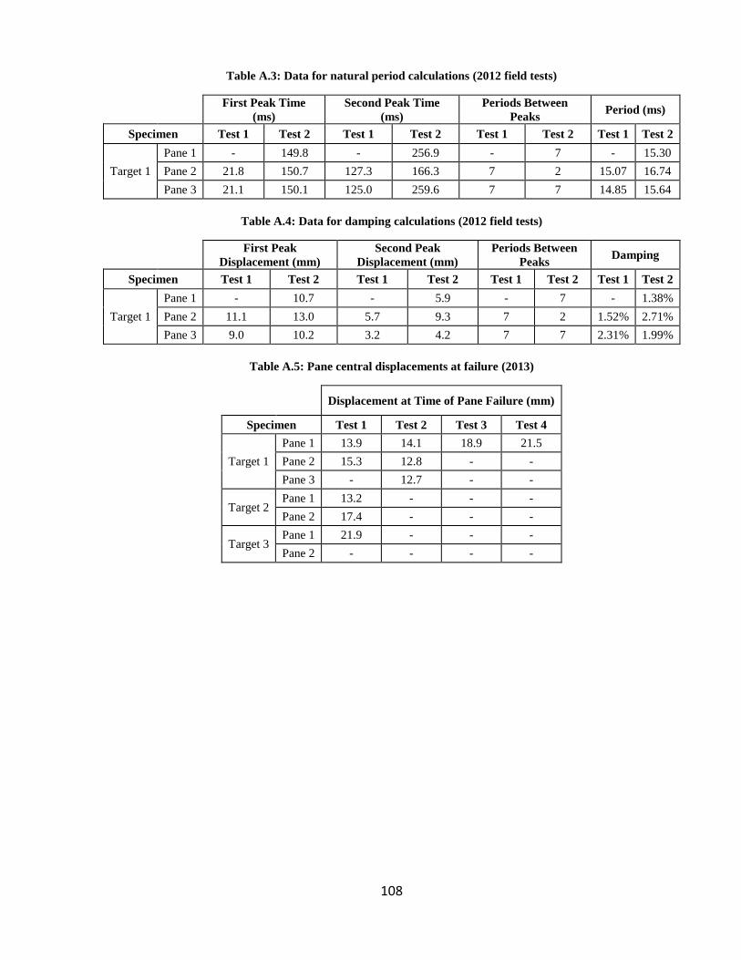
108

Table A.3: Data for natural period calculations (2012 field tests)

First Peak Time

(ms)

Second Peak Time

(ms)

Periods Between

Peaks Period (ms)

Specimen Test 1 Test 2 Test 1 Test 2 Test 1 Test 2 Test 1 Test 2

Target 1

Pane 1 - 149.8 - 256.9 - 7 - 15.30

Pane 2 21.8 150.7 127.3 166.3 7 2 15.07 16.74

Pane 3 21.1 150.1 125.0 259.6 7 7 14.85 15.64

Table A.4: Data for damping calculations (2012 field tests)

First Peak

Displacement (mm)

Second Peak

Displacement (mm)

Periods Between

Peaks Damping

Specimen Test 1 Test 2 Test 1 Test 2 Test 1 Test 2 Test 1 Test 2

Target 1

Pane 1 - 10.7 - 5.9 - 7 - 1.38%

Pane 2 11.1 13.0 5.7 9.3 7 2 1.52% 2.71%

Pane 3 9.0 10.2 3.2 4.2 7 7 2.31% 1.99%

Table A.5: Pane central displacements at failure (2013)

Displacement at Time of Pane Failure (mm)

Specimen Test 1 Test 2 Test 3 Test 4

Target 1

Pane 1 13.9 14.1 18.9 21.5

Pane 2 15.3 12.8 - -

Pane 3 - 12.7 - -

Target 2 Pane 1 13.2 - - -

Pane 2 17.4 - - -

Target 3 Pane 1 21.9 - - -

Pane 2 - - - -

109

Appendix B: Small-Scale Testing Data

Table B.1: Beam specimen type testing results

Specimen Type Specimen

Failure

Load

(kN)

Failure Stress

(MPa)

Average Failure

Stress (MPa)

Location of

Critical Flaw

1

No processing

1-1 3.84 109.4

97.0

Middle

1-2 3.05 82.5 Middle

1-3 3.49 98.9 Middle

2

Edges ground

and polished

2-1 2.31 65.0

57.3

Edge

2-2 1.92 54.1 Edge

2-3 1.89 52.7 Edge

3

Corners chamfered

3-1 2.79 55.3

64.8

Middle

3-2 2.60 70.3 Middle

3-3 2.47 68.9 Middle

4

Edges ground

and polished,

corners chamfered

4-1 2.82 79.4

72.8

Edge

4-2 2.36 64.2 Edge

4-3 2.68 74.9 Edge

Table B.2: Average four-point bending failure stress for each pane and cut direction

Average Failure Stress (MPa)

Cut Direction Pane 1 Pane 2 Pane 3 Pane 4

1 77.4 75.3 98.4 84.1

2 80.6 83.3 76.3 82.7

110

Table B.3: Full four-point bending results, 2012 glass

PaneCut

DirectionSpecimen

Failure

Load

(kN)

Failure

Stress

(MPa)

Central

Deflection

(mm)

Tensile Strain

(10-3

)

Compressive

Strain (10-3

)

E, Deflection

(MPa)

E, Strain

(MPa)

Load

Rate

(MPa/s)

Fracture

Location

(mm from

end 1)

Failure

Type

3 1 31 1-1 4.54 131.4 -1.40 1.78 - 72100 73300 1.29 93 Edge

3 1 31 1-2 4.43 124.6 -1.33 2.09 -0.72 72100 75000 1.28 141 Edge

3 1 31 1-3 2.98 82.0 -0.87 1.10 -1.10 70900 73600 1.22 122 Face

3 1 31 1-4 4.43 126.5 -1.37 1.71 -1.72 71400 74200 1.29 89 Edge

3 1 31 1-5 2.82 82.0 -0.87 1.07 -1.06 73100 76300 1.21 152 Edge

3 1 31 1-6 2.73 74.9 -0.79 0.98 -0.97 73100 76200 1.21 121 Face

3 1 31 1-7 4.59 129.2 -1.57 - - 63800 - 1.11 122 Face

3 1 31 1-8 3.87 109.7 -1.24 - - 70000 - 1.19 168 Face

3 1 31 1-9 4.63 129.1 -1.41 - - 70100 - 1.26 96 Edge

3 1 31 1-10 4.02 99.4 -1.27 - - 67900 - 1.06 180 Face

3 1 31 1-11 3.43 95.2 -1.03 - - 71800 - 1.22 110 Face

3 1 31 1-12 4.09 71.4 -1.29 - - 71500 - 0.68 195 Edge

3 2 32 1-1 2.35 67.7 -0.72 0.89 -0.89 72100 76000 1.19 174 Face

3 2 32 1-2 2.64 72.4 -0.79 0.98 -0.97 70500 73900 1.17 90 Face

3 2 32 1-3 2.05 57.1 -0.61 0.75 -0.75 71900 75500 1.09 121 Face

3 2 32 1-4 2.53 70.7 -0.80 -0.96 0.97 67600 72800 1.12 104 Face

3 2 32 1-5 2.75 77.4 -0.85 1.05 -1.05 70500 73200 1.16 74 Face

3 2 32 1-6 2.82 78.9 -0.85 1.14 -1.04 72100 72400 1.18 173 Edge

3 2 32 1-7 3.86 112.2 -1.23 - - 70500 - 1.22 157 Face

3 2 32 1-8 2.88 78.7 -0.91 - - 67300 - 1.08 103 Edge

3 2 32 1-9 3.78 86.0 -1.19 - - 67700 - 0.95 184 Edge

3 2 32 1-10 2.72 75.8 -0.83 - - 68600 - 1.11 90 Edge

3 2 32 1-11 3.38 96.7 -0.99 - - 74600 - 1.24 117 Edge

4 1 41 1-1 3.95 109.9 -1.17 - - 71800 - 1.26 93 Face

4 1 41 1-2 2.68 73.7 -0.77 0.95 -0.95 72300 76900 1.20 140 Face

4 1 41 1-3 3.13 83.8 -0.91 1.13 -1.10 69600 75600 1.20 173 Face

4 1 41 1-5 2.92 79.1 -0.88 1.11 -1.07 68300 72300 1.15 175 Face

4 1 41 1-6 2.84 79.0 -0.86 1.05 - 69400 74500 1.20 85 Face

4 1 41 1-7 1.96 53.5 -0.64 - - 72100 - 1.13 168 Face

4 1 41 1-8 3.13 84.7 -0.95 - - 73300 - 1.24 101 Edge

4 1 41 1-9 3.27 85.9 -0.94 - - 72600 - 1.22 73 Face

4 1 41 1-10 2.83 76.0 -0.81 - - 70500 - 1.20 79 Edge

4 1 41 1-11 3.96 109.4 -1.12 - - 73100 - 1.32 82 Face

4 1 41 1-12 3.03 82.5 -0.87 - - 71400 - 1.26 123 Face

4 2 42 1-1 3.14 85.9 -0.95 1.04 -1.10 69100 79600 1.16 90 Face

4 2 42 1-2 3.73 106.0 -1.15 1.36 -1.39 71700 76800 1.25 130 Face

4 2 42 1-3 3.23 90.2 -0.99 1.20 - 70000 74800 1.18 91 Edge

4 2 42 1-4 3.07 82.3 -0.89 1.09 -0.98 70400 78100 1.17 167 Edge

4 2 42 1-5 2.92 68.5 -0.88 1.11 -1.07 71400 62500 0.99 183 Face

4 2 42 1-6 3.52 98.0 -1.03 1.27 - 72700 76700 1.26 157 Face

4 2 42 1-7 3.17 87.9 -0.93 - - 71100 - 1.26 76 Face

4 2 42 1-8 2.88 79.3 -0.85 - - 70600 - 1.22 131 Face

4 2 42 1-9 4.16 113.6 -1.20 - - 71300 - 1.31 133 Edge

4 2 42 1-10 1.91 53.0 -0.59 - - 69000 - 1.10 77 Face

4 2 42 1-11 2.77 70.6 -0.85 - - 67600 - 1.15 71 Edge

111

Table B.4: Full four-point bending results, 2013 glass

Sample

TypePane

Cut

DirectionSpecimen

Failure

Load

(kN)

Failure

Stress

(MPa)

Central

Deflection

(mm)

Tensile Strain

(10-3)

Compressive

Strain (10-3)

E, Deflection

(MPa)

E, Strain

(MPa)

Load

Rate

(MPa/s)

Fracture

Location

(mm from

end 1)

Failure

Type

X 1 1-1 3.84 100.7 1.14 1.44 -1.43 72900 70100 0.31 179 Face

X 1 1-2 3.05 82.5 0.88 -1.10 1.13 69900 -73500 0.31 95 Face

X 1 1-3 3.49 98.9 0.99 - - - - 0.33 143 Face

1 1 11 1-1 3.02 84.2 0.90 - - 71100 - 1.25 133 Edge

1 1 11 1-2 3.59 89.3 1.05 - - 71500 - 0.99 179 Face

1 1 11 1-3 2.65 71.4 0.82 - - 68800 - 1.07 147 Face

1 1 11 1-4 2.24 59.8 0.66 - - 69800 - 1.05 122 Edge

1 1 11 1-5 2.07 57.0 0.62 - - 70500 - 1.13 137 Face

1 1 11 1-6 3.09 85.3 0.89 - - 71700 - 1.35 102 Face

1 1 11 1-7 2.37 63.1 0.68 - - 72000 - 1.11 80 Edge

1 1 11 1-8 2.90 78.1 0.82 1.03 -1.02 72100 75700 1.17 94 Face

1 1 11 1-9 3.13 83.6 0.89 1.06 -0.52 73500 120100 1.18 176 Face

1 1 11 1-10 2.91 77.2 0.81 - - 71200 - 1.17 170 Face

1 2 12 1-2 3.30 88.6 0.98 - - 70000 - 1.17 125 Face

1 2 12 1-3 3.57 95.9 0.99 - - 73400 - 1.24 168 Face

1 2 12 1-4 3.59 94.3 1.01 - - 69900 - 1.24 141 Face

1 2 12 1-5 2.95 81.4 0.84 - - 74200 - 1.22 94 Face

1 2 12 1-8 2.52 67.2 0.54 0.89 -0.88 93500 76300 1.15 141 Face

1 2 12 1-9 3.00 80.4 -0.84 0.02 - 72400 - 1.18 107 Edge

1 2 12 1-10 2.19 56.1 -0.63 0.80 -0.77 70000 74000 1.03 177 Face

2 1 21 1-1 3.45 92.6 1.02 - - 69200 - 1.18 113 Face

2 1 21 1-2 3.53 94.1 1.01 - - 71100 - 1.22 134 Face

2 1 21 1-3 3.34 90.4 1.00 - - 69000 - 1.04 85 Face

2 1 21 1-4 2.62 69.5 0.77 - - 68800 - 1.15 160 Face

2 1 21 1-5 2.30 62.8 0.67 - - 72600 - 1.10 127 Face

2 1 21 1-6 3.29 88.9 0.85 - - 78700 - 1.22 88 Edge

2 1 21 1-7 2.34 64.5 0.71 - - 69900 - 1.17 89 Face

2 1 21 1-8 2.20 59.4 -0.64 0.78 -0.76 69900 76500 1.09 88 Face

2 1 21 1-9 2.54 69.3 -0.75 0.93 -0.89 69700 75600 1.12 117 Face

2 1 21 1-10 2.44 66.7 -0.71 -0.08 -0.86 72500 69000 1.09 115 Edge

2 2 22 1-1 2.95 79.9 0.69 - - 74200 - 1.21 103 Face

2 2 22 1-2 3.23 87.9 0.73 - - 78300 - 1.23 128 Face

2 2 22 1-3 3.90 113.9 1.00 - - 84500 - 1.40 174 Edge

2 2 22 1-5 3.81 102.6 1.09 - - 71000 - 1.23 135 Face

2 2 22 1-6 2.29 62.1 0.66 - - 71400 - 1.20 110 Edge

2 2 22 1-7 2.98 78.8 0.85 - - 68900 - 1.20 114 Face

2 2 22 1-8 2.79 74.4 -0.81 0.99 -0.99 69500 74800 1.14 113 Face

2 2 22 1-9 2.82 78.2 -0.81 0.01 -0.99 72900 194000 1.19 93 Edge

2 2 22 1-10 2.81 76.3 -0.81 1.01 -0.75 70800 88200 1.16 117 Face

X 1 2-1 2.31 65.0 0.68 0.29 -0.85 70900 144900 1.24 122 Edge

X 1 2-2 1.92 54.1 0.55 0.69 -0.68 73900 78000 1.20 172 Edge

X 1 2-3 1.89 52.7 0.53 0.67 -0.64 73600 78700 1.32 81 Edge

X 1 3-1 2.79 55.3 0.83 1.03 -1.02 53200 75900 1.39 148 Face

X 1 3-2 2.60 70.3 0.75 0.93 -0.93 70000 73600 1.29 140 Face

X 1 3-3 2.47 68.9 0.75 0.94 -0.86 69600 75300 1.28 89 Face

X 1 4-1 2.82 76.4 0.82 1.03 -1.02 72300 73000 1.30 177 Edge

X 1 4-2 2.36 64.2 0.67 0.78 -0.83 70900 77600 1.30 155 Edge

X 1 4-3 2.68 75.6 0.79 0.99 -0.97 71800 75300 1.34 81 Edge

1 1 11 4-1 2.71 73.4 - - - - - 1.21 137 Edge

1 1 11 4-2 2.28 63.9 0.66 - - 73800 - 1.18 102 Face

1 1 11 4-3 2.14 56.5 0.59 - - 71600 - 1.13 80 Face

1 2 12 4-1 2.28 64.8 0.66 - - 74800 - 1.19 151 Edge

1 2 12 4-2 3.07 84.4 0.87 - - 73400 - 1.26 75 Edge

1 2 12 4-3 3.20 86.6 0.90 - - 72800 - 1.28 90 Edge

2 1 21 4-1 3.13 86.8 0.91 - - 72500 - 1.25 87 Face

2 1 21 4-2 3.07 85.6 0.87 - - 74500 - 1.27 133 Face

2 1 21 4-3 3.20 89.1 0.90 - - 75200 - 1.32 100 Face

2 2 22 4-2 2.95 85.0 0.89 - - 71600 - 1.28 174 Face

2 2 22 4-3 2.88 79.7 0.83 - - 72200 - 1.22 128 Edge

1

2

3

4

112

Table B.5: Full three-point bending results, 2013 glass

PaneCut

DirectionSpecimen

Failure

Load

(kN)

Failure

Stress

(MPa)

Central

Deflection

(mm)

E, Deflection

(MPa)

Load

Rate

(MPa/s)

Fracture

Location

(mm from

end 1)

Failure

Type

5 1 51 1-1 1.79 86.2 -0.750 71000 0.781 135 Face

5 1 51 1-2 1.87 89.4 -0.773 70300 0.767 135 Face

5 1 51 1-3 0.98 50.7 -0.391 70300 1.058 128 Face

5 1 51 1-4 1.63 84.0 -0.701 69600 1.005 132 Face

5 1 51 1-5 1.71 87.3 -0.699 71500 1.063 130 Edge

5 1 51 1-6 2.34 119.2 -0.953 72100 1.074 119 Edge

5 1 51 1-7 1.34 65.2 -0.562 71800 0.957 137 Face

5 1 51 1-8 1.61 81.8 -0.679 70900 1.008 132 Edge

5 1 51 1-9 1.85 82.5 -0.770 70700 0.894 142 Face

5 1 51 1-10 0.85 44.8 -0.354 70700 1.048 127 Face

5 1 51 1-11 1.32 69.0 -0.542 71800 1.059 129 Edge

5 1 51 1-12 1.87 99.4 -0.779 70000 1.084 125 Face

5 1 51 1-13 1.75 69.1 -0.724 71300 0.805 152 Edge

5 1 51 1-14 1.38 58.6 -0.576 73500 0.849 102 Face

5 2 52 1-1 2.16 94.7 -0.898 71300 0.904 144 Face

5 2 52 1-2 1.59 70.8 -0.693 72100 0.865 103 Edge

5 2 52 1-3 1.52 73.5 -0.647 69900 0.946 135 Edge

5 2 52 1-4 1.17 59.1 -0.481 71300 1.021 131 Face

5 2 52 1-5 2.81 138.7 -1.173 70800 1.028 134 Face

5 2 52 1-6 2.15 112.9 -0.902 70800 1.069 128 Face

5 2 52 1-7 2.32 67.2 -0.964 71300 0.599 171 Face

5 2 52 1-8 2.02 69.0 -0.849 70500 0.693 162 Face

5 2 52 1-9 1.64 82.8 -0.671 70400 1.019 130 Face

5 2 52 1-10 1.90 63.7 -0.784 70400 0.683 162 Face

5 2 52 1-11 1.83 62.8 -0.762 70000 0.700 160 Face

5 2 52 1-12 1.58 78.5 -0.646 73200 1.014 133 Face

5 2 52 1-13 1.51 67.8 -0.649 71300 0.865 144 Face

5 2 52 1-14 2.10 93.7 -0.780 69800 1.032 131 Edge

6 1 61 1-1 1.82 92.9 -0.752 70600 1.039 119 Edge

6 1 61 1-2 2.00 81.4 -0.845 71200 0.867 149 Face

6 1 61 1-3 1.63 82.0 -0.686 70600 1.032 118 Face

6 1 61 1-4 1.25 58.8 -0.513 71800 0.959 138 Face

6 1 61 1-5 1.48 67.4 -0.610 71400 0.954 141 Edge

6 1 61 1-6 2.23 100.4 -0.928 71100 0.935 142 Face

6 1 61 1-7 1.96 69.5 -0.814 70600 0.750 91 Edge

6 1 61 1-8 1.89 94.2 -0.764 71500 1.062 133 Edge

6 1 61 1-9 1.75 89.9 -0.723 70000 1.086 122 Face

6 1 61 1-10 1.26 65.8 -0.504 71900 1.073 127 Face

6 1 61 1-11 1.62 69.8 -0.684 68000 0.887 107 Face

6 1 61 1-12 1.35 66.4 -0.523 73100 1.040 116 Edge

6 1 61 1-13 1.11 59.7 -0.426 77100 1.134 128 Face

6 1 61 1-14 1.10 52.4 -0.431 62700 0.973 125 Face

6 2 62 1-1 1.63 77.7 -0.676 71400 0.992 113 Face

6 2 62 1-2 2.01 107.0 -0.818 71600 1.134 123 Face

6 2 62 1-3 2.31 82.5 -0.984 69200 0.735 160 Face

6 2 62 1-4 1.33 65.4 -0.542 71300 1.027 117 Face

6 2 62 1-5 1.73 93.4 -0.742 71800 1.100 122 Face

6 2 62 1-6 1.88 86.7 -0.773 71300 0.976 139 Face

6 2 62 1-7 1.24 65.6 -0.503 71100 1.076 122 Edge

6 2 62 1-8 1.03 47.7 -0.403 71900 0.968 138 Edge

6 2 62 1-9 1.63 85.5 -0.687 71900 1.075 130 Face

6 2 62 1-10 2.37 127.3 -1.012 69800 1.124 123 Face

6 2 62 1-11 2.13 109.6 -0.897 70200 1.076 120 Face

6 2 62 1-12 1.82 77.7 -0.759 71400 0.880 148 Face

6 2 62 1-13 1.89 96.0 -0.778 71000 1.074 120 Face

6 2 62 1-14 1.66 88.8 -0.673 71800 1.138 125 Face

113

Table B.6: Flaw size data

Specimen

Mirror Radius

(mm)

(rM)

Crack Half Length

(mm)

(b)

Crack Length

(mm)

(2b)

Failure Stress

(MPa)

(σ)

A

(MPa-m1/2

)

11 1-2 0.594 0.0594 0.119 89.3 2.177

11 1-3 0.655 0.0655 0.131 71.4 1.828

11 1-4 0.902 0.0902 0.180 59.8 1.795

11 1-5 1.122 0.1122 0.224 57.0 1.908

11 1-6 0.579 0.0579 0.116 85.3 2.052

11 1-8 0.637 0.0637 0.127 78.1 1.971

11 1-10 0.681 0.0681 0.136 77.2 2.014

12 1-2 0.551 0.0551 0.110 88.6 2.080

12 1-3 0.449 0.0449 0.090 95.9 2.032

12 1-4 0.474 0.0474 0.095 94.3 2.054

12 1-5 0.738 0.0738 0.148 81.4 2.212

12 1-8 0.990 0.0990 0.198 67.2 2.115

21 1-1 0.425 0.0425 0.085 92.6 1.910

21 1-3 0.390 0.0390 0.078 90.4 1.785

21 1-7 1.299 0.1299 0.260 64.5 2.325

21 1-8 1.294 0.1294 0.259 59.4 2.138

21 1-9 0.894 0.0894 0.179 69.3 2.071

22 1-1 0.720 0.0720 0.144 79.9 2.144

22 1-2 0.607 0.0607 0.121 87.9 2.165

22 1-5 0.390 0.0390 0.078 102.6 2.028

22 1-7 0.639 0.0639 0.128 78.8 1.993

22 1-8 0.772 0.0772 0.154 74.4 2.068

22 1-9 0.709 0.0709 0.142 78.2 2.081

22 1-10 0.796 0.0796 0.159 76.3 2.153

31 1-3 0.605 0.0605 0.121 82.0 2.016

31 1-6 0.787 0.0787 0.157 74.9 2.102

31 1-7 0.232 0.0232 0.046 129.2 1.967

31 1-8 0.388 0.0388 0.078 109.7 2.160

31 1-10 0.407 0.0407 0.081 99.4 2.005

31 1-11 0.443 0.04425 0.089 95.2 2.004

32 1-1 1.048 0.10484 0.210 67.7 2.192

32 1-2 0.711 0.07111 0.142 72.4 1.931

32 1-3 1.414 0.14135 0.283 57.1 2.148

32 1-4 0.760 0.076005 0.152 70.7 1.949

32 1-5 0.686 0.06857 0.137 77.4 2.027

32 1-7 0.351 0.035135 0.070 112.2 2.103

41 1-1 0.316 0.031645 0.063 109.9 1.955

41 1-2 0.881 0.08806 0.176 73.7 2.187

41 1-3 0.572 0.057205 0.114 83.8 2.005

41 1-7 1.516 0.15157 0.303 53.5 2.085

41 1-9 0.596 0.05957 0.119 85.9 2.096

41 1-12 0.617 0.061725 0.123 82.5 2.050

42 1-1 0.520 0.052025 0.104 85.9 1.959

42 1-7 0.534 0.053405 0.107 87.9 2.031

42 1-8 0.630 0.062995 0.126 79.3 1.990

114

42 1-10 1.784 0.178385 0.357 53.0 2.238

51 1-3 1.718 0.171785 0.344 50.7 2.100

51 1-4 0.528 0.05279 0.106 84.0 1.931

51 1-7 1.000 0.09998 0.200 65.2 2.062

51 1-9 0.566 0.05659 0.113 82.5 1.963

51 1-10 2.513 0.251275 0.503 44.8 2.244

51 1-12 0.419 0.04188 0.084 99.4 2.034

51 1-14 1.513 0.15126 0.303 58.6 2.279

52 1-1 0.452 0.045185 0.090 94.7 2.013

52 1-4 1.223 0.122305 0.245 59.1 2.067

52 1-6 0.321 0.032135 0.064 112.9 2.024

52 1-7 0.929 0.092945 0.186 67.2 2.050

52 1-8 0.993 0.099305 0.199 69.0 2.175

52 1-9 0.547 0.05471 0.109 82.8 1.936

52 1-10 1.046 0.10462 0.209 63.7 2.060

52 1-12 0.731 0.073125 0.146 78.5 2.124

52 1-13 0.804 0.08039 0.161 67.8 1.923

61 1-2 0.620 0.06201 0.124 81.4 2.028

61 1-3 0.612 0.06115 0.122 82.0 2.027

61 1-4 1.248 0.124825 0.250 58.8 2.076

61 1-6 0.388 0.03878 0.078 100.4 1.977

61 1-9 0.515 0.051515 0.103 89.9 2.040

61 1-10 1.041 0.10411 0.208 65.8 2.123

61 1-11 0.853 0.085345 0.171 69.8 2.038

61 1-13 1.532 0.1532 0.306 59.7 2.337

62 1-1 0.640 0.06402 0.128 77.7 1.966

62 1-2 0.330 0.032995 0.066 107.0 1.944

62 1-3 0.681 0.06808 0.136 82.5 2.154

62 1-5 0.488 0.048835 0.098 93.4 2.064

62 1-6 0.515 0.051535 0.103 86.7 1.968

62 1-9 0.571 0.057085 0.114 85.5 2.044

62 1-10 0.254 0.02543 0.051 127.3 2.030

62 1-13 0.442 0.04424 0.088 96.0 2.020

62 1-14 0.484 0.04843 0.097 88.8 1.953

1-2 0.523 0.05227 0.105 82.5 1.886

1-3 0.425 0.042545 0.085 98.9 2.041

3-1 0.733 0.07329 0.147 55.3 1.498

3-2 0.872 0.087185 0.174 70.3 2.075

3-3 0.820 0.082045 0.164 68.9 1.974

11 4-2 1.130 0.113 0.226 63.9 2.148

11 4-3 1.451 0.14513 0.290 56.5 2.151

21 4-1 0.590 0.05898 0.118 86.8 2.108

21 4-2 0.856 0.08562 0.171 85.6 2.505

22 4-3 1.007 0.100705 0.201 68.6 2.176

115

Appendix C: Large-Scale Testing Data

Table C.1: Data for natural period calculations (large-scale testing)

Test # First Peak Time (s) Second Peak Time (s) Number of Periods Between Peaks Period (ms)

1 - - - -

2 1.92 2.07 7 22.2

3 1.22 1.39 8 21.6

4 2.00 2.13 6 20.9

5 1.99 2.09 5 21.2

6 1.08 1.21 6 21.0

7 1.54 1.68 7 20.6

8 1.42 1.57 7 20.9

9 1.08 1.23 7 21.9

10 1.40 1.54 7 20.7

1 1.81 1.95 6 23.2

2 1.89 2.03 6 24.2

3 1.46 1.55 4 21.5

4 1.63 1.72 4 22.1

5 1.34 1.45 5 22.2

6 1.47 1.58 5 22.6

7 1.60 1.73 6 22.0

8 0.84 0.91 3 22.0

9 1.40 1.53 6 22.3

10 1.88 1.99 5 21.8

11 1.26 1.34 4 21.6

12 2.30 2.41 5 21.0

13 3.42 3.58 7 21.7

14 2.33 2.42 4 21.5

15 3.41 3.52 5 22.0

16 4.45 4.56 5 22.1

116

Table C.2: Data for damping calculations (large-scale testing)

Test First Amplitude Time

(mm)

Second Peak Amplitude

(mm)

Number of Periods Between

Peaks Damping

1 - - - -

2 0.235 0.036 7 4.24%

3 0.215 0.028 8 4.07%

4 0.126 0.031 6 3.75%

5 0.111 0.025 5 4.74%

6 0.131 0.032 6 3.75%

7 0.104 0.019 7 3.82%

8 0.125 0.023 7 3.88%

9 0.206 0.027 7 4.62%

10 0.128 0.035 7 2.96%

11 0.334 0.044 6 5.35%

12 0.443 0.046 6 6.04%

13 0.158 0.057 4 4.06%

14 0.223 0.065 4 4.92%

15 0.179 0.038 5 4.96%

16 0.196 0.059 5 3.79%

17 0.170 0.040 6 3.85%

18 0.194 0.080 3 4.67%

19 0.213 0.051 6 3.81%

20 0.201 0.044 5 4.82%

21 0.168 0.098 4 2.13%

22 0.141 0.039 5 4.10%

23 0.207 0.036 7 3.94%

24 0.147 0.072 4 2.84%

25 0.189 0.059 5 3.69%

26 0.193 0.064 5 3.49%

117

Figure C.1: Large-scale testing principal strains (test 1)

Figure C.2: Large-scale pane central strains (test 1)

118

Figure C.3: Large-scale pane central strains (test 2)

Figure C.4: Large-scale pane edge strains (test 1)

119

Figure C.5: Large-scale pane edge strains (test 2)

120

Appendix D: Blast Modelling Data

Figure D.1: SBEDS metal plate template input (2013, test 1, Target 1)

121

Figure D.2: SBEDS generic SDOF template input, dynamic resistance function (2013, test 1, Target 1)

Figure D.3: WINGARD material property input (2013, test 1, Target 1)

122

Figure D.4: WINGARD glass layup input (2013, test 1, Target 1)

Figure D.5: WINGARD window system input (2013, test 1, Target 1)

123

Figure D.6: CWBlast geometry input (2013, test 1, Target 1)

Figure D.7: CWBlast material property input (2013, test 1, Target 1)

124

Figure D.8: CWBlast support condition input (2013, test 1, Target 1)

Figure D.9: CWBlast load input (2013, test 1, Target 1)

125

Figure D.10: CWBlast failure criteria input (2013, test 1, Target 1)

126

Figure D.11: Measured and predicted pane central displacements (2013, test 1, Target 1)


127



Response of Annealed Glass Windows to Blast Loads · Table 3.2: Blast wave peak positive reflected...

Documents

Transcript of Response of Annealed Glass Windows to Blast Loads · Table 3.2: Blast wave peak positive reflected...