
Resource-saving operation and control of stainless steel ... · Resource-saving operation and...
31
Resource-saving operation and control of stainless steel refining in VOD and AOD Processes - EUR 25087 Mikael Ersson
Transcript of Resource-saving operation and control of stainless steel ... · Resource-saving operation and...

Resource-saving operation and control of stainless steel refining in VOD and AOD Processes - EUR 25087Mikael Ersson

Background
This RFCS project started in 2010, it was a collaboration between:
BFIKTHSMS MevacKobolde & PartnersAcroniOutokumpu Stainless

Background
KTH performed numerical modeling of the VOD at Acroni and of the AOD in Avesta.
BFI, SMS and Kobolde worked with dynamic process models of the VOD and AOD, as well as with data acquisition for those models.
This presentation will naturally focus on the numerical aspects of this project.
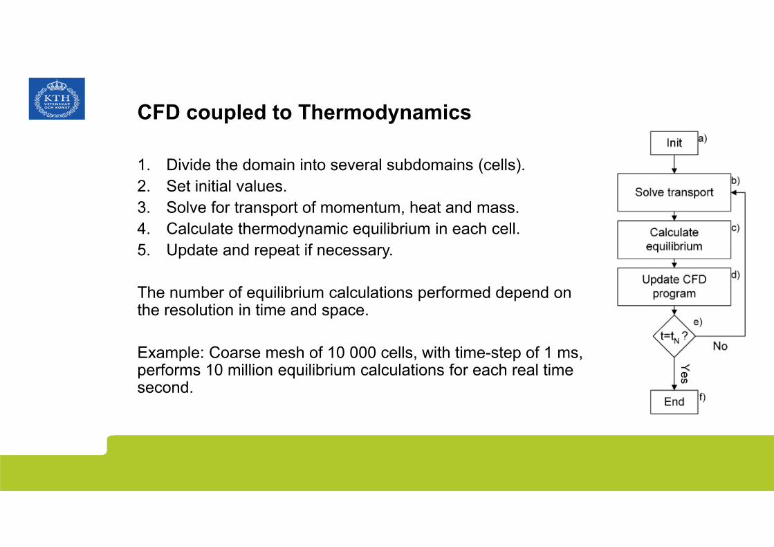
CFD coupled to Thermodynamics
1. Divide the domain into several subdomains (cells).2. Set initial values.3. Solve for transport of momentum, heat and mass.4. Calculate thermodynamic equilibrium in each cell.5. Update and repeat if necessary.
The number of equilibrium calculations performed depend on the resolution in time and space.
Example: Coarse mesh of 10 000 cells, with time-step of 1 ms, performs 10 million equilibrium calculations for each real time second.

The AOD numerical model
The converter in Avesta was modeled with the following assumptions:
3-D with symmetry along the center.
The free surface is flat and bubbles can leave through it freely.
The injection takes place through 3 nozzles and gas instantaneously takes the steel temperature.

The AOD numerical model
Furthermore:
Liquid temperature is taken from the TimeAOD2 model of Kobolde.
The slag phase is homogeneous and treated as liquid spherical droplets. The initial slag height is 6.3 cm.
5 Thermo-Calc database elements (Ar, C, Cr, Fe, O)
15 extra scalar transport equations (5 per phase)

Stirring pattern in the Avesta AOD
Snapshot of the velocity vectors, close to the symmetry plane.
The flow field is not stationary!

Results AOD modeling

CFD results, compared to the TimeAOD2 process model
Decarburization vs time for different bath temperatures
~72 kg/min
~96 kg/min

Results AOD modeling
How fast is the mixing in the AOD converter?
The oxygen is turned off and replaced with inert gas, keeping the total flow rate constant.
The concentration is thenhomogenized over time.

Results AOD modeling

Results AOD modeling
The coupled CFD-Thermodynamics solution gives decarburization results comparable to the TimeAOD process model.
Mixing phenomena can be extracted from the simulation. In particular, the mixing time, which for the AOD in Avesta is approximately 30 seconds.
Even with this fast mixing time there are clearly visible concentration gradientsin the converter during decarburization.

The VOD numerical model
2-D axisymmetrical model
9 Thermo-Calc database elements (Ar,C,Cr,Ca,Fe,N,Ni,O,S)
3 phases (Steel, Slag and Gas)
27 extra scalar transport equations (9 for each phase)
Time-step approximately 0.01 ms.
Millions of thermodynamic equilibrium calculations for 5 minutes of simulation.
Initial data

Results VOD modeling
Results VOD modeling
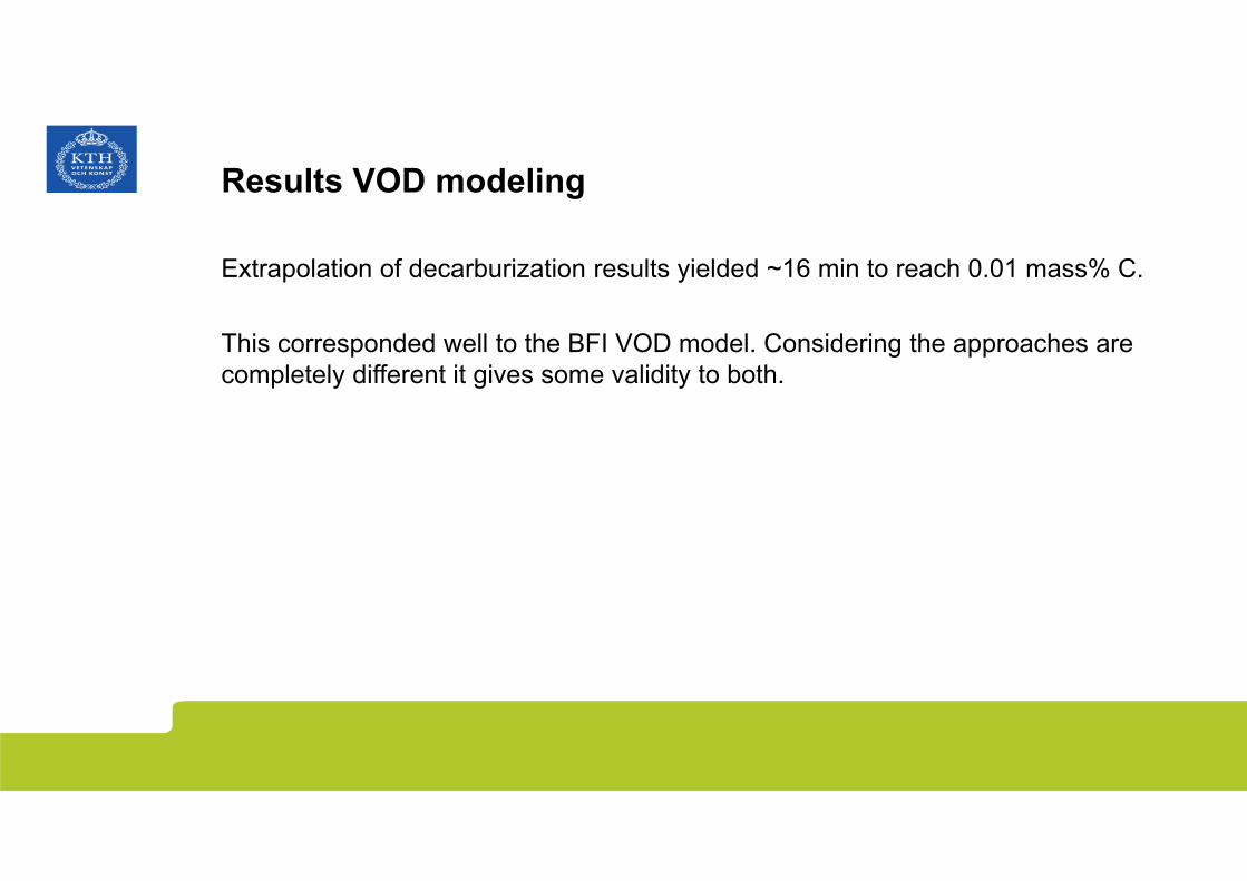
Extrapolation of decarburization results yielded ~16 min to reach 0.01 mass% C.
This corresponded well to the BFI VOD model. Considering the approaches are completely different it gives some validity to both.

Results VOD modeling

Results VOD modeling
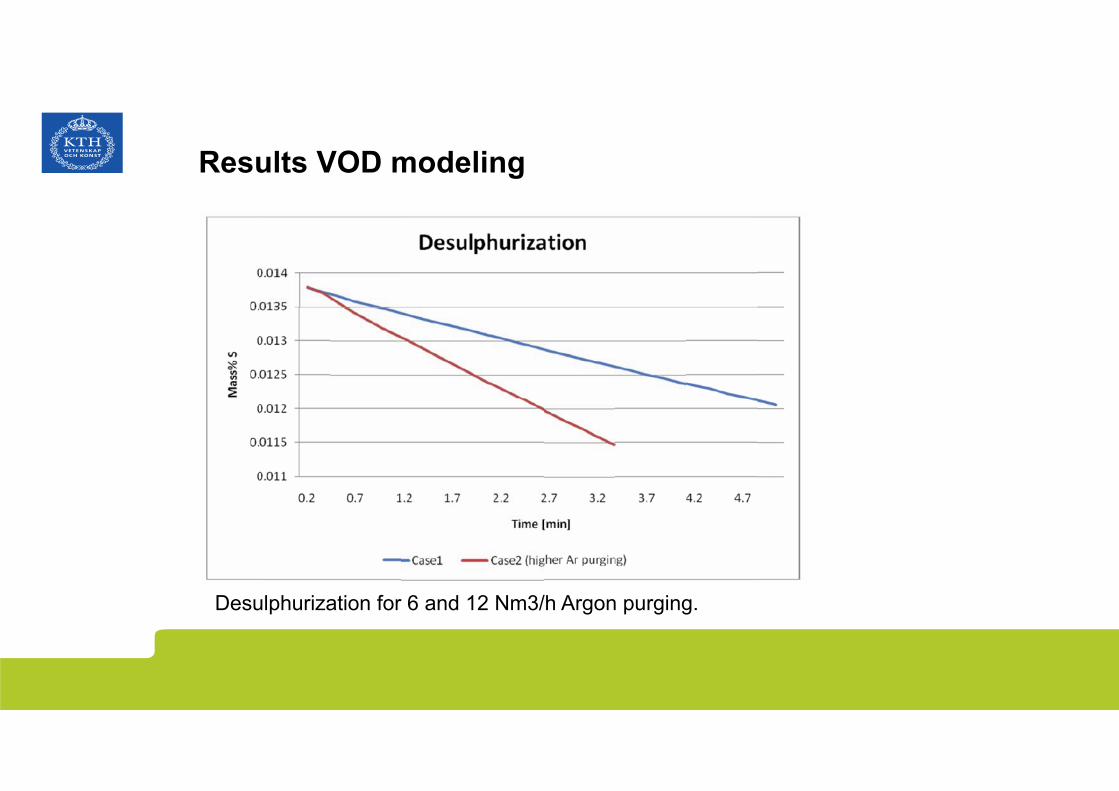
Desulphurization for 6 and 12 Nm3/h Argon purging.
Results VOD modeling
Desulphurization for 6 and 12 Nm3/h Argon purging.

Results VOD modeling – Vacuum pressure
Standard:110 mbar – 5mbar/min
High pressure:220 mbar – 10 mbar/min

Results VOD modeling – Vacuum pressure
Standard:110 mbar – 5mbar/min
High pressure:220 mbar – 10 mbar/min

Results VOD modeling – Vacuum pressure
Standard:110 mbar – 5mbar/min
High pressure:220 mbar – 10 mbar/min

Results VOD modeling – Vacuum pressure
Decarburization and Chromium oxidation is not largely affected by an increased vacuum pressure.
This is also confirmed by experimental measurements of SMS Mevac and Acroni at the Acroni plant, as well as by the dynamic VOD model of BFI.
In other words: it may be possible to save money by running vacuum pumps at lower power.

Results VOD modeling – nozzle configuration
Nozzle type A Nozzle type B
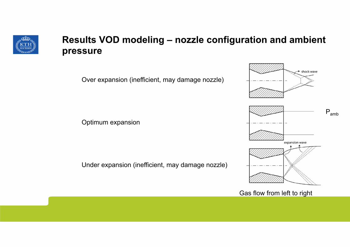
Results VOD modeling – nozzle configuration and ambient pressure
Over expansion (inefficient, may damage nozzle)
Optimum expansion
Under expansion (inefficient, may damage nozzle)
Gas flow from left to right
Pamb

Results VOD modeling – nozzle configuration, jet velocity

Results VOD modeling – nozzle configuration, jet velocity

Results VOD modeling – nozzle configuration, jet force
Ambient pressure has a large impact on the force.
Temperature has almost no impact!
Force evaluated at 1.3 m from the nozzle (initial position of bath surface)

Results VOD modeling – nozzle configuration, jet force
The jet force at 1.3 meters after the nozzle (initial position of bath surface)
Lower pressures favor Nozzle B and higher pressures favor Nozzle A.
Nozzle A is also cheaper to manufacture.

Summary
The CFD models were able to predict parts of the AOD and VOD processes.
The results were validated against process models which were trimmed to the specific plants.
The methodology of using CFD coupled to Thermodynamic databases show great promise as a fundamental tool to investigate high temperature phenomena in steel production.

Thank you!

Results VOD modeling – Nitrogen pick-up