Resource location based on precomputed partial random...
16
Computer Networks 103 (2016) 165–180 Contents lists available at ScienceDirect Computer Networks journal homepage: www.elsevier.com/locate/comnet Resource location based on precomputed partial random walks in dynamic networks Víctor M. López Millán a,∗ , Vicent Cholvi b,1 , Antonio Fernández Anta d,2 , Luis López c,3 a Universidad CEU San Pablo, Spain b Universitat Jaume I, Spain c Universidad Rey Juan Carlos, Spain d Institute IMDEA Networks, Spain a r t i c l e i n f o Article history: Received 23 November 2015 Revised 29 February 2016 Accepted 9 April 2016 Available online 13 April 2016 Keywords: Resource location Dynamic networks Random walks Complex networks a b s t r a c t The problem of finding a resource residing in a network node (the resource location problem) is a chal- lenge in complex networks due to aspects as network size, unknown network topology, and network dynamics. The problem is especially difficult if no requirements on the resource placement strategy or the network structure are to be imposed, assuming of course that keeping centralized resource informa- tion is not feasible or appropriate. Under these conditions, random algorithms are useful to search the network. A possible strategy for static networks, proposed in previous work, uses short random walks precomputed at each network node as partial walks to construct longer random walks with associated resource information. In this work, we adapt the previous mechanisms to dynamic networks, where re- source instances may appear in, and disappear from, network nodes, and the nodes themselves may leave and join the network, resembling realistic scenarios. We analyze the resulting resource location mecha- nisms, providing expressions that accurately predict average search lengths, which are validated using simulation experiments. Reduction of average search lengths compared to simple random walk searches are found to be very large, even in the face of high network volatility. We also study the cost of the mechanisms, focusing on the overhead implied by the periodic recomputation of partial walks to refresh the information on resources, concluding that the proposed mechanisms behave efficiently and robustly in dynamic networks. © 2016 Published by Elsevier B.V. 1. Introduction Random walks are network routing mechanisms which have been extensively studied and used in a wide range of applica- tions: physics, mathematics, population dynamics, bioinformatics, etc. [11,18,24]. Roughly speaking, they choose, at each point of the ∗ Corresponding author. Tel.: +34 91 3726424 (ext. 4911); fax: +34 91 3724049. E-mail address: [email protected] (V.M.L. Millán). 1 Supported in part by the Spanish Ministerio de Economía y Competitividad un- der grant TIN2011-28347-C02-01. 2 Supported in part by Ministerio de Economia y Competitividad grant TEC2014- 55713-R, Regional Government of Madrid (CM) grant Cloud4BigData (S2013/ICE- 2894, co-funded by FSE & FEDER), NSF of China grant 61520106005, and European Commission H2020 grants ReCred and NOTRE. 3 Supported in part by the European Commission under projects NUBOMEDIA (FP7-ICT GA 610576), FI-WARE (FP7-ICT GA 285248) and FI-CORE (FP7-ICT GA 632893). This work is also supported by the Spanish Ministerio de Economía y Competitividad under grant REACTIVEMEDIA (TIN2013-41819-R) and by Comunidad de Madrid under grant CLOUD4BIGDATA (P2013/ICE-2894) cofounded by FSE & FEDER. route, the next node uniformly at random among the neighbors of the current node. Among the advantages of random walks when applied to communication networks is the fact they need only local informa- tion, avoiding the bandwidth overhead necessary in other routing mechanisms to communicate with other nodes. This is especially useful when there is no knowledge on the structure of the whole network, or when the network structure changes frequently. For these reasons, random walks have been proposed as a base mechanism for multiple network applications, including network sampling [9,16], network resource location [1,10,28,33], network construction [5,15,19–21], and network characterization [8,29,32]. The emergence of the peer-to-peer (P2P) architecture model has been proven useful in many applications in recent years. While structured P2P systems (e.g., Chord [31], CAN [27] –Content- Addressable Network–, Kademlia [23], etc.) provide efficient search mechanisms, they introduce a significant management overhead. In turn, unstructured systems have little management overhead and, consequently, have been considered in several scenarios (e.g., Gnutella [5,20], CAP [14] –Cluster-based Architecture for P2P–, http://dx.doi.org/10.1016/j.comnet.2016.04.008 1389-1286/© 2016 Published by Elsevier B.V.
Transcript of Resource location based on precomputed partial random...

Computer Networks 103 (2016) 165–180
Contents lists available at ScienceDirect
Computer Networks
journal homepage: www.elsevier.com/locate/comnet
Resource location based on precomputed partial random walks in
dynamic networks
Víctor M. López Millán
a , ∗, Vicent Cholvi b , 1 , Antonio Fernández Anta
d , 2 , Luis López
c , 3
a Universidad CEU San Pablo, Spain b Universitat Jaume I, Spain c Universidad Rey Juan Carlos, Spain d Institute IMDEA Networks, Spain
a r t i c l e i n f o
Article history:
Received 23 November 2015
Revised 29 February 2016
Accepted 9 April 2016
Available online 13 April 2016
Keywords:
Resource location
Dynamic networks
Random walks
Complex networks
a b s t r a c t
The problem of finding a resource residing in a network node (the resource location problem ) is a chal-
lenge in complex networks due to aspects as network size, unknown network topology, and network
dynamics. The problem is especially difficult if no requirements on the resource placement strategy or
the network structure are to be imposed, assuming of course that keeping centralized resource informa-
tion is not feasible or appropriate. Under these conditions, random algorithms are useful to search the
network. A possible strategy for static networks, proposed in previous work, uses short random walks
precomputed at each network node as partial walks to construct longer random walks with associated
resource information. In this work, we adapt the previous mechanisms to dynamic networks, where re-
source instances may appear in, and disappear from, network nodes, and the nodes themselves may leave
and join the network, resembling realistic scenarios. We analyze the resulting resource location mecha-
nisms, providing expressions that accurately predict average search lengths, which are validated using
simulation experiments. Reduction of average search lengths compared to simple random walk searches
are found to be very large, even in the face of high network volatility. We also study the cost of the
mechanisms, focusing on the overhead implied by the periodic recomputation of partial walks to refresh
the information on resources, concluding that the proposed mechanisms behave efficiently and robustly
in dynamic networks.
© 2016 Published by Elsevier B.V.
1
b
t
e
d
5
2
C
(
6
C
d
F
r
t
c
t
m
h
1
. Introduction
Random walks are network routing mechanisms which have
een extensively studied and used in a wide range of applica-
ions: physics, mathematics, population dynamics, bioinformatics,
tc. [11,18,24] . Roughly speaking, they choose, at each point of the
∗ Corresponding author. Tel.: +34 91 3726424 (ext. 4911); fax: +34 91 3724049.
E-mail address: [email protected] (V.M.L. Millán). 1 Supported in part by the Spanish Ministerio de Economía y Competitividad un-
er grant TIN2011-28347-C02-01. 2 Supported in part by Ministerio de Economia y Competitividad grant TEC2014-
5713-R, Regional Government of Madrid (CM) grant Cloud4BigData (S2013/ICE-
894, co-funded by FSE & FEDER), NSF of China grant 61520106005, and European
ommission H2020 grants ReCred and NOTRE. 3 Supported in part by the European Commission under projects NUBOMEDIA
FP7-ICT GA 610576), FI-WARE (FP7-ICT GA 285248) and FI-CORE (FP7-ICT GA
32893). This work is also supported by the Spanish Ministerio de Economía y
ompetitividad under grant REACTIVEMEDIA (TIN2013-41819-R) and by Comunidad
e Madrid under grant CLOUD4BIGDATA (P2013/ICE-2894) cofounded by FSE &
EDER.
u
n
F
m
s
c
h
W
A
m
I
a
G
ttp://dx.doi.org/10.1016/j.comnet.2016.04.008
389-1286/© 2016 Published by Elsevier B.V.
oute, the next node uniformly at random among the neighbors of
he current node.
Among the advantages of random walks when applied to
ommunication networks is the fact they need only local informa-
ion, avoiding the bandwidth overhead necessary in other routing
echanisms to communicate with other nodes. This is especially
seful when there is no knowledge on the structure of the whole
etwork, or when the network structure changes frequently.
or these reasons, random walks have been proposed as a base
echanism for multiple network applications, including network
ampling [9,16] , network resource location [1,10,28,33] , network
onstruction [5,15,19–21] , and network characterization [8,29,32] .
The emergence of the peer-to-peer (P2P) architecture model
as been proven useful in many applications in recent years.
hile structured P2P systems (e.g., Chord [31] , CAN [27] –Content-
ddressable Network–, Kademlia [23] , etc.) provide efficient search
echanisms, they introduce a significant management overhead.
n turn, unstructured systems have little management overhead
nd, consequently, have been considered in several scenarios (e.g.,
nutella [5,20] , CAP [14] –Cluster-based Architecture for P2P–,

166 V.M.L. Millán et al. / Computer Networks 103 (2016) 165–180
1
a
u
[
a
(
(
n
h
S
S
t
r
t
w
t
s
i
S
a
1 A round is a unit of discrete time in which every node is allowed to send a
message to one of its neighbors. According to this definition, a simple random walk
of length � would then take � rounds to be computed.
etc.). For such systems, searching techniques based on flooding, su-
pernodes and random walks have been used. However, it is known
that flooding mechanisms do not scale well [13] , and supernode
systems are vulnerable to supernodes failures (technical problems,
attacks, censorship, etc.). Therefore, random walks have been used
to search for resources held in the nodes of a network (e.g., [5,22] ),
a problem usually known as resource location . The problem con-
sists of finding a node that holds a given resource, the target node ,
starting at some source node . The source node is checked for the
resource: if it is not found locally, the search hops to a random
neighbor, checking that node for the resource. The search proceeds
through the network in this way, until the target node is reached.
Nevertheless, by using random walks, some nodes may be (un-
necessarily) visited more than once, while other nodes may remain
unvisited for a long time. Avoiding this problem is the main objec-
tive of our study.
1.1. The Dynamic resource location problem
In this work, we are concerned with the resource location prob-
lem in networks with dynamic behavior regarding both resources
and nodes.
In particular, we consider scenarios in which resources are ran-
domly placed in the nodes across the network. Then, on the one
hand, we consider scenarios in which the instances of the re-
sources may appear and disappear from a time instant to another,
maybe at different nodes. On the other hand, we also consider sce-
narios in which the network nodes themselves may also leave and
join the network.
In these scenarios, all the nodes of the network may launch in-
dependent searches for different resources (e.g., files) at any time,
without the help of a centralized server, and we are interested in
measuring the average performance of searches between any pair
of nodes.
Our assumptions regarding dynamicity cover a wide range of
scenarios. For instance, in P2P networks nodes represent users,
which may leave and join the network quite often. Also, resources
represent the shared files, which may appear and disappear from
time to time.
1.2. Contributions
In this work, we use the technique of concatenating partial
random walks (PWs) to generalize the resource location mecha-
nisms introduced in [17] for static networks to the case of dy-
namic networks. In particular, this paper provides new analytical
models that predict the behavior of the resource location mecha-
nisms in scenarios with dynamic resources and in scenarios with
dynamic nodes, along with new simulation experiments to validate
the analytical results. In addition, a new analysis of the cost of the
mechanisms in these scenarios is provided. We consider the two
versions of the mechanisms proposed in [17] and adapt them to
operate in the dynamic scenarios. In the first version, which we
refer as choose-first PW-RW , the search mechanism first chooses
one of the PWs at random and then checks its associated infor-
mation for the desired resource. In the second version, which we
refer as check-first PW-RW , the search mechanism first checks the
associated resource information of all the PWs of the node, and
then randomly chooses among the PWs with a positive result. It is
clear that there are other choices regarding the search mechanisms
that seem reasonable. However, the ones considered in our study
follow very different approaches (one chooses first, and the other
checks first). Therefore, that will allow us to check the strength of
our approach in very different circumstances.
Then, we have studied their performance, considering the fol-
lowing aspects:
• Dynamic resources: We have developed an analytical mean-field
model for both mechanisms when resources are dynamic. Ex-
pressions are given for the corresponding expected search length
(i.e., the expected number of hops taken to find the resource,
averaged over all source nodes, target nodes, and network
topologies) of each mechanism. These expressions provide pre-
dictions as a function of several parameters of the model, such
as the network structure (size and degree distribution), the re-
source dynamics, and those of the mechanisms operation.
The predictions of the models are validated by simulation ex-
periments in three types of randomly built networks: regular,
Erd ̋os-Rényi, and scale-free. These experiments are also used to
compare the performance of both mechanisms, and to inves-
tigate the influence of the resource dynamics. We have com-
pared the performance of the proposed search mechanisms
with respect to random walk searches. For the choose-first PW-
RW mechanism we have found a reduction in the average
search length with respect to simple random walk ranging from
around 57% to 88%. For the check-first PW-RW mechanism such
a reduction is even bigger, achieving reductions above 90%.
• Dynamic nodes: We have also considered the case where net-
work nodes may leave and join the network, and have pro-
vided both analytical and experimental results. We have found
a reduction in the average search length with respect to simple
random walks above 94% (using the check-first PW-RW mecha-
nism).
• Cost: Finally, we have analyzed the cost of the PW-RW mecha-
nisms, defined as the number of messages, taking into account
the cost of searches themselves and the cost of precomputing
the PWs in each recomputation interval. We have provided an-
alytical expressions for the relation between the cost and the
length of the recomputation interval, as well as for the interval
length that minimizes this cost. We have found that the impact
of the precomputation of PWs on the cost is not significant in a
wide range of lengths of the precomputation interval depending
on the dynamic behavior of the network and on the dynamic
behavior of searches.
.3. Related work
Da Fontoura Costa and Travieso [6] study the network cover-
ge of three types of random walks: traditional, preferential to
ntracked edges, and preferential to unvisited nodes. Also, Yang
33] studies the search performance of five random walk vari-
tions: no-back (NB), no-triangle-loop (NTL), no-quadrangle-loop
NQL), self-avoiding (SA) and high-degree-preferential self-avoiding
PSA). Self-avoiding walks (SAW) are those that try not to visit
odes that have already been visited. Several variations of this idea
ave been studied, differing in the probability of revisiting a node.
ome examples are: strict SAW, true or myopic SAW, and weakly
AW [4,30] . In [7] , Das Sarma et al. propose a distributed algorithm
o obtain a random walk of a specified length � in a number of
ounds 1 proportional to √
� .
López Millán et al [17] propose a mechanism for resource loca-
ion based on building random walks connecting together partial
alks (PW) previously computed at each network node. However,
he mechanisms in [17] are only valid when both nodes and re-
ources have a static behavior, contrary to the approach we follow
n this paper.
The remainder of this paper is arranged as follows.
ection 2 and 3 respectively present the choose-first PW-RW
nd check-first PW-RW mechanisms in scenarios with dynamic

V.M.L. Millán et al. / Computer Networks 103 (2016) 165–180 167
r
w
e
p
2
l
s
N
l
s
t
f
s
a
f
t
g
i
r
t
n
s
t
m
i
L
r
a
T
w
s
t
a
i
a
p
u
a
r
l
o
p
i
b
T
n
fi
f
r
t
i
n
t
Fig. 1. Example of the dynamic behavior of resources. The network is shown at
t =0 (left hand side), when the PWs are precomputed, and at time t = T (right
hand side), the end of the PW recomputation interval. The resource instances have
changed during the interval.
esources. Section 4 adapts the previous mechanisms to scenarios
ith dynamic nodes. In Section 6 , the cost of the mechanisms is
valuated in dynamic scenarios. Finally, Section 7 concludes this
aper and provides some future work lines.
. Choose-first PW-RW with dynamic resources
Consider a communication network (e.g., the Internet, a wire-
ess ad-hoc network, etc.) that provides full connectivity to the end
ystem entities (e.g., computers, smartphones, etc.) connected to it.
ext, consider a subset of N end system entities which establish
ogical neighboring relations for some purpose (a P2P file sharing
ystem, a social network application, etc.). These end system en-
ities (as the nodes ) and their neighboring relations (as the links )
orm an overlay network on top of the underlying network . 2 The re-
ource location mechanisms described in this paper apply to such
n overlay network (referred to simply as the network ), and we will
ocus on searches for resources in the end system entities (referred
o as the nodes ).
Each of the N nodes holds a set of resources. We focus on a
iven resource of interest, of which initially there is a number of
nstances randomly placed in many distinct network nodes. Our
esource location problem is defined as finding one of the nodes
hat hold the resource (the one we encounter first, called the target
ode ), starting by a certain node (the source node ). We make no as-
umption on the underlying communication network, focusing on
he number of nodes of the overlay visited to find a resource, as a
easure of search performance.
In our analysis, for each search, we assume that the source node
s uniformly chosen at random among all nodes in the network.
ikewise, we consider that the instances of the resource have been
andomly distributed throughout the network. The probability that
given node holds an instance of the resource is denoted by p res .
he expected number of instances of the resource for a given net-
ork is denoted by R = N · p res .
Resources have a dynamic behavior. If we compared two snap-
hots of the network, one taken at time t =0 and another taken at
ime t =T , we would observe that some of the instances have dis-
ppeared while other new ones have appeared (at different nodes,
n general). More concretely, an instance present in a node dis-
ppears with probability d . Conversely, an instance not initially
resent in a node appears in that node with probability a . We will
se d as an input parameter to characterize resource dynamics. For
value of d , we will set a so that expectation of the number of
esources ( R ) remains unchanged. This way, our results will iso-
ate the impact of resource dynamics on the search mechanism due
nly to the deterioration of information, discarding the effect of a
ossible increase or decrease on the expected number of resource
nstances. Fig. 1 provides an illustrative example of the dynamic
ehavior of the resources.
he search mechanism. A search performs a walk from the source
ode to the target node according to the mechanism that is de-
ned below. The search mechanism proposed in this paper, re-
erred to as PW-RW, exploits the idea of efficiently building total
andom walks from partial random walks available at each node of
he network. It comprises two stages:
1. Partial random walks construction : In an initial stage at time
t =0 , every node i in the network precomputes a set W i of w
random walks before the searches take place, with the initial
2 Note that neighbors in the overlay are not in general neighbors in the underly-
ng network. Note also that the underlying communication network provides con-
ectivity between any pair of end system entities, even if they are not neighbors in
he overlay.
distribution of resource instances in the network. Each of these
partial walks (PW) has length s , starting at i and finishing at a
node reached after s hops. Using the PW-RW mechanisms, the
PWs computed in this stage are simple random walks (i.e., the
next node to be visited is chosen uniformly at random among
the neighbors of the current node).
During the computation of each PW in W i , node i registers the
resources held by the s first nodes in the PW (from i to the
one before the last node). The last node of the PW is excluded,
being included in the PWs departing from it. In particular, for
each PW computed by i , this node keeps the set of the identi-
fiers of the resources held by the nodes in that PW. In this set,
there is no indication of the particular node or nodes holding
the resource. The registered information will be used by the
searches in stage 2, to decide whether to traverse that PW (if
the resource looked for is found in the set of identifiers), or to
jump over it (if the resource is not found).
2. The searches : During the interval 0 < t ≤ T , after the PWs are
constructed, searches are performed in the network. We will
consider the system at t =T , in which, as stated above, the
dynamic behavior of resource instances is characterized by d .
Therefore, results obtained will reflect the performance of the
search mechanism in a worst case scenario, since searches exe-
cuted in t < T will see a probability that an instance disappears
less than or equal to d . There is no relation between the inter-
val T , measured in time units, and the hops of a search, other
than the assumption that T is much longer than the duration of
a typical search, as discussed later in this section in paragraph
Resource dynamics .
A search can be qualitatively described as a sequence of jumps
over PWs, interleaved with some occassional unsuccessful PW
traversals, and finished by the successful traversal of a PW un-
til the target node is visited. Unsuccessful PW traversals are
caused by outdated resource information associated to that PW,
i.e., the resource was in the PW at t = 0 but it has disappeared
at the time of the search. The last PW traversal will be incom-
plete in general, in the sense that its length will be less than or
equal to s , since the search stops when the resource is found.
We measure the length of searches in hops . Some of these hops
are jumps (over PWs), and other are steps (traversing PWs).
We distinguish between unnecessary steps (in unsuccessful PW
traversals), and final steps (in the last, successful, PW). The def-
inition of the search mechanism and the associated concepts
are illustrated by the example in Fig. 2 , in which PWs of length
s = 6 are used.
At this point, we emphasize the difference between the search
just defined and the total walk that supports it. Indeed, the
total walk consist of the concatenation of partial walks as de-
fined above. Searches are therefore shorter in length than their

168 V.M.L. Millán et al. / Computer Networks 103 (2016) 165–180
Fig. 2. An example search: total walk, partial walks, jumps and steps.
Table 1
Resource dynamics: query results.
Resource present in PW
case t = 0 t = T Query result
a) no no True Negative (TN)
b) yes yes True Positive (TP)
c) no yes False Negative (FN)
d) yes no False Positive (FP)
Fig. 3. Resource dynamics: examples of results when a PW precomputed at t =0 is
queried at t =T .
p
i
i
s
i
F
w
i
i
w
a
t
c
p
i
a
l
s
t
s
P
i
O
q
w
a
i
T
b
l
e
corresponding total walks because of the number of steps saved
in jumps over PWs in which we know that the resource is not
located, although these saving may be reduced by the unneces-
sary steps due to outdated information within PWs.
More formally, we describe how searches are performed as fol-
lows. Let a search start at a node A . A PW in W A is chosen uni-
formly at random. Its associated resource information collected
in stage 1 is then queried for (any instance of) the desired re-
source.
• If the query result is negative (i.e., the resource is not in
the set of identifiers associated with that PW), the search
jumps to node B , the last node of that PW. Note that the cur-
rent node and the node to which the search jumps are not
neighbors in the overlay network in general. Jumps there-
fore make use of the underlying communication network.
The process is then repeated at B and the search keeps
jumping in this way while the results of the queries are neg-
ative.
• If the query result is positive (i.e., the resource is in the set
of identifiers), the search traverses that PW looking for the
resource. It starts checking if the current node has the de-
sired resource. If it does not, the search takes a step to the
next node of the PW, checking again if it has the resource.
The search proceeds through the PW in this way until the
resource is found or the PW is finished.
– If the resource is found, the search stops.
– Otherwise (i.e., the search reaches the last node of the
PW without having found the resource in the previous
nodes), it means that the information collected in stage
1 for that PW and the resource of interest is no longer
valid. The search considers that the result is negative,
and the search process is repeated at the last node of
the PW.
Resource dynamics. Regarding resource dynamics, we realize that
searches are executed based on information collected at t =0 that
may be outdated during the interval 0 < t ≤ T , when the queries
are performed. The duration of the interval ( T ) is assumed to be
much longer than the duration of a typical search, since we are in-
terested in using the PWs computed at t = 0 for as many searches
as possible, with an acceptable degradation of information associ-
ated with those PWs. 3 Therefore, most of the searches take place
within the interval, and only a few start in one interval and finish
in the following interval. The part of those searches in the follow-
ing interval benefits from the newly computed PWs of this inter-
val. Our analysis will consider that all searches take place within
the interval, thus reflecting a worst case situation. Four cases arise
when the information associated with a PW is queried for the re-
source, as is shown in Table 1 and illustrated by Fig. 3 .
3 A discussion of the optimal duration of the interval is provided in Section 6 .
l
s
r
A True Negative or TN (case a) occurs when no instances were
resent in the PW at t =0 , and the same holds at t =T . A True Pos-
tive or TP (case b) occurs when one or more instances are present
n the PW at t =0 and one or more instances (not necessarily the
ame ones) are present at t =T . The impact of resource dynam-
cs on the performance of the search mechanism comes from the
alse Negatives (FN) and the False Positives (FP). A FN (case c) occurs
hen there were no instances in the PW at t =0 , but at least one
nstance is present at t =T . It makes the search jump over that PW,
gnoring the new instance(s). An FP (case d) occurs when there
ere one or more instances in that PW at t =0 but all of them
re gone at t =T and there are no new instances at t =T . It makes
he search traverse a whole PW fruitlessly, since no instances are
urrently in that PW. Note that the case when all instances disap-
ear from the PW, but some other instance(s) appears in that PW
s included in the TP case.
At this point, we note that the performance of the search mech-
nism can be affected by the degradation of the information col-
ected in the PWs. For instance, if all the instances of a given re-
ource disappear and new instances appear in nodes that happen
o be in PWs which did not have the resource at t = 0 , the re-
ource would not be found, since searches would jump over those
Ws due to the (false) negative result of the queries. Therefore,
n order to keep their accuracy, PWs may need to be “refreshed”.
nce the interval is finished, PWs are recomputed at t =T to ac-
uire fresh resource information, and searches from t =T to t =2 T
ill use the new PWs. In other words, stages 1 and 2 described
bove are repeated with a period T . In Section 6 , we assess the
mpact of this PW recomputation on the overall searches cost.
he search metrics. In this work, we are interested in the num-
er of hops to find a resource, which is defined as the search
ength . This search length is a random variable that takes differ-
nt values when independent searches are performed. The search
ength distribution is defined as the probability distribution of the
earch length random variable. So, the expected search length , de-
ived from the mentioned distribution, taken over all networks, all

V.M.L. Millán et al. / Computer Networks 103 (2016) 165–180 169
s
s
a
R
a
e
p
a
s
e
b
2
o
t
a
s
i
T
e
f
n
t
I
P
n
P
e
w
l
s
L
w
w
r
T
e
l
L
L
p
P
t
r
P
s
p
r
4 This probability p tp is not to be confused with P tp (note the different case), de-
fined above as the probability of choosing a PW which returns a TP out of the w
PWs of the current node.
ource nodes, and target nodes, is an interesting performance mea-
ure of the searching mechanism in a given network.
In the next section we provide an analytical model that gives
n estimation of the expected search length of the choose-first PW-
W mechanism. We use a mean-field model and analysis. In this
pproach, instead of computing the search length distribution for
ach network, source node and target node, and then taking ex-
ectations, the analysis itself handles average values. Whereas this
pproach may not accurately reflect some border cases (like some
pecific network topologies), it captures rather accurately the gen-
ral characteristics and metrics of the mechanisms. This fact has
een also confirmed by using simulations.
.1. Analysis
Since we have defined the expected search length for any pair
f source and target nodes, the expected length of the search from
he source node is the same as the expected search length from
ny subsequent node in the search. This allows us to write a recur-
ive expression for the expected search length. Consider the search
s at some node i , one of whose PWs is queried for the resource.
he expected search length from i can be written in terms of the
xpected search length from the next node j that will be queried
or the resource, plus the number of hops taken from node i to
ode j . If the result of the query at i was negative (either false or
rue), the search will jump from i to j , adding 1 hop to the search.
f the result was a false positive, the search will traverse the entire
W without finding the resource, adding s hops to the search. Fi-
ally, if the result was a true positive, the search will traverse the
W until the resource is found, adding a number of hops whose
xpected value we call F . These cases occur with probabilities that
e call, respectively: P n , P tp , and P fp . Denoting the expected search
ength using PWs of length s by L s , the resulting recursive expres-
ion is then:
s = ( L s + 1) · P n + ( L s + s ) · P fp + F · P tp , (1)
here P n , P tp , and P fp are the probabilities of choosing a partial
alk (out of the w PWs of the node) for which the query for the
esource returns a negative (either a TN or a FN, see Table 1 ), a
P, and an FP result, respectively, with P n + P tp + P fp = 1 . F is the
xpectation of the number of final steps taken when traversing the
ast PW, until an instance of the resource is found (TP). Solving for
s , we obtain:
s =
1
P tp · (P n + s · P fp ) + F . (2)
The probabilities in Eq. 2 are estimated with the following ex-
ressions:
P tp =
w ∑
i =1
w −i ∑
j=0
P (i, j) · i
w
,
fp =
w −1 ∑
i =0
w −i ∑
j=1
P (i, j) · j
w
,
P n =
w −1 ∑
i =0
w −i −1 ∑
j=0
P (i, j) · w − (i + j)
w
= 1 − P tp − P fp , (3)
where P ( i, j ) is the probability that, in the w PWs of a node,
here are i PWs whose queries return a TP result and j PWs that
eturn an FP result:
(i, j) = B (w, p tp , i ) · B (w − i, p fp , j) , (4)
where
• B ( m, q, n ) is the coefficient of the binomial distribution
B (m, q, n ) =
(m
n
)· q n · (1 − q ) (m −n ) , (5)
• p tp is the probability that a given PW at any node returns a TP
result, 4
• and p fp is the probability that a given PW at any node returns
an FP result, conditioned on the fact that it does not return
a TP.
Therefore, in order to evaluate the estimation of the expected
earch length given by Eq. 2 , we need to obtain the values of p tp ,
fp and F . Let us provide them:
1. The variable p tp has been defined as the probability that a given
PW at any node returns a TP result. This probability can be
easily estimated if we condition it on the fact that the PW (of
length s ) had exactly r instances of the resource at t =0 . Defin-
ing P pw
( r ) as the probability that a PW has r instances of the
resource, and recalling that R is the expectation of the number
of instances of the resource in the network, we can write:
p tp =
min { s, R } ∑
r=1
P pw
(r) · [(1 − d r ) + d r · (1 − (1 − a ) s −r )] , (6)
where the brackets contain the probability that not all the r in-
stances present at t =0 have disappeared (with probability d )
at t =T or, if they did disappear, at least one instance appeared
(with probability a ) in some of the s − r remaining nodes in
that interval.
An estimation for P pw
( r ) can be obtained using the random
properties of a random walk in networks built randomly. In par-
ticular, we consider that the next hop of a random RW can take
it to any of the endpoints in the network (except the endpoints
of the current node since we do not allow self-loops). Then we
estimate P pw
( r ) as B ( s, p rw
, r ), where p rw
is the probability that
the RW visits a node with an instance of the resource in the
next hop. In turn, we estimate this probability as:
p rw
=
R · k
S − k rw
· k rw
− 1
k rw
. (7)
The first fraction in Eq. 7 is the ratio of positive endpoints (the
ones connected to the R nodes that have an instance of the re-
source) and all endpoints in the network ( S =
∑
k k n k ) except
those of the current node. We use the average degree of the
network ( k =
∑
k k n k /N) as an estimation of the degree of a
node that holds the resource (which is assigned or not with
uniform probability p res across the network). Similarly, we use
the expectation of the degree of a node visited by a random
walk as an estimation of the degree of the current node:
k rw
=
∑
k
k · k · n k
S =
1
S ·∑
k
k 2 · n k . (8)
The second fraction in Eq. 7 corrects the previous ratio taking
into account that, when at a node of a given degree, the proba-
bility of not going backwards (and therefore having the chance
to find the resource) is the probability of selecting any of its
endpoints but the one that connects it with the node just vis-
ited by the walk. With this, the estimation of P pw
( r ) is:
P pw
(r) =
(s )
· (p rw
) r · (1 − p rw
) s −r . (9)
170 V.M.L. Millán et al. / Computer Networks 103 (2016) 165–180
t
0
20
40
60
80
100
120
140
0 50 100 150 200 250 300 350 400
expe
cted
sea
rch
leng
th (
hops
)
partial walks length (hops)
choose-first PW-RW
dynamic resources
scale-free network
d=0.7 (simul)(model)
d=0.5 (simul)(model)
d=0.3 (simul)(model)
d=0.1 (simul)(model)
d=0.0 (simul)(model)
Fig. 4. Choose-first PW-RW with dynamic resources: expected search length L s vs.
PW length s for several d in a scale-free network.
Table 2
Choose-first PW-RW with dynamic resources: reduction of the expected
search lengths relative to RW searches for several d .
Search length
d reduction (%)
0 .0 88 .28
0 .1 86 .37
0 .3 81 .23
0 .5 72 .94
0 .7 57 .26
c
f
d
t
2
w
b
o
s
t
a
a
h
S
P
l
d
t
2
m
(
l
5 The extreme case of having just one PW is to be avoided because it yields many
unfinished searches, since it is relatively easy to build walks that are loops that do
not cover the network. Indeed, if the last node of a PW is a node whose (only) PW
has been already used in that total walk, it will take the search to the same place
again, resulting in a never-ending loop.
2. We have defined p fp as the probability that a given PW at any
node returns an FP result, conditioned on the fact that it does
not return a TP. This conditioning comes from the second bino-
mial coefficient in this equation, which we restrict to the w − i
PWs which we know that do not return a TP, since the ones
that do are accounted for in the first binomial coefficient. In
other words, the second binomial coefficient includes the PWs
that return a TN, a FN or an FP result, and p fp is the probability
that it returns an FP conditioned on that. We can then easily
write an estimation of p fp as:
p fp =
1
1 − p tp ( 1 − P pw
(0) − p tp ) , (10)
where we are substracting P pw
(0) (the probability of cases TN
and FN in Table 1 ), and p tp (the probability of case TP).
3. An expression for F , the expectation of the number of final
steps taken when traversing the last PW until an instance of
the resource is found, is still needed to be finally able to es-
timate the average search length in Eq. 2 . For this we rely on
F (r) , the expectation of that variable conditioned on there be-
ing r instances of the resource in the PW. Then:
F =
1
1 − P pw
(0) ·
min { s, R } ∑
r=1
F (r) · P pw
(r) . (11)
Note that F is in fact conditioned on there being at least one
instance of the resource in the PW, since it corresponds to a TP
(see Eq. 1 ). This is the reason of the fraction multiplying the
summation in Eq. 11 .
Now we provide an expression for F (r) as the expectation of
the position of the first resource in the PW (conditioned on
there being r instances of the resource in the PW):
F (r) =
s −r ∑
i =0
[
i ·(
i −1 ∏
j=0
(1 − r
s − j
))
·(
r
s − i
)]
. (12)
Each factor in the product of Eq. 12 is the probability that there
is no instance in the jth position of the PW, conditioned on that
there is no instance in the previous position. The final factor
outside the product is the probability that there is an instance
in the i th position conditioned on there are no instances in the
previous positions.
2.2. Performance evaluation
In this section, we apply the model presented in the previ-
ous section to real networks, and we also validate its predictions
with data obtained from simulations. Three types of networks have
been chosen for the experiments: regular networks (constant node
degree), Erd ̋os-Rényi (ER) networks and scale-free networks (with
power law on the node degree). These topologies cover a wide va-
riety of real networks [3] , ranging from communication networks
[2] to Internet [26] and P2P networks [12] .
A network of each type and size N = 10 4 has been randomly
built with the method proposed by Newman et al. [25] for net-
works with arbitrary degree distribution, setting their average
node degree to k = 10 . Each network is constructed in three steps:
(1) a preliminary network is constructed according to its type; (2)
its degree distribution is extracted, and (3) the final network is ob-
tained feeding the referenced method with that degree distribu-
tion. For each experiment, 10 6 searches have been performed. In
every search, the source node has been chosen uniformly at ran-
dom, and every node in the network has been assigned an in-
stance of the resource looked for with probability p res = 10 −2 at
=0 . Therefore, the expected number of resource instances present
in the network at t =0 for all searches is R = N · p res = 100 .
We show the results for scale-free networks, which are espe-
ially interesting since this type of degree distribution is frequently
ound in real networks. Results for regular and ER networks, which
o not differ significantly from scale-free results, are included in
he Appendix for the interested reader.
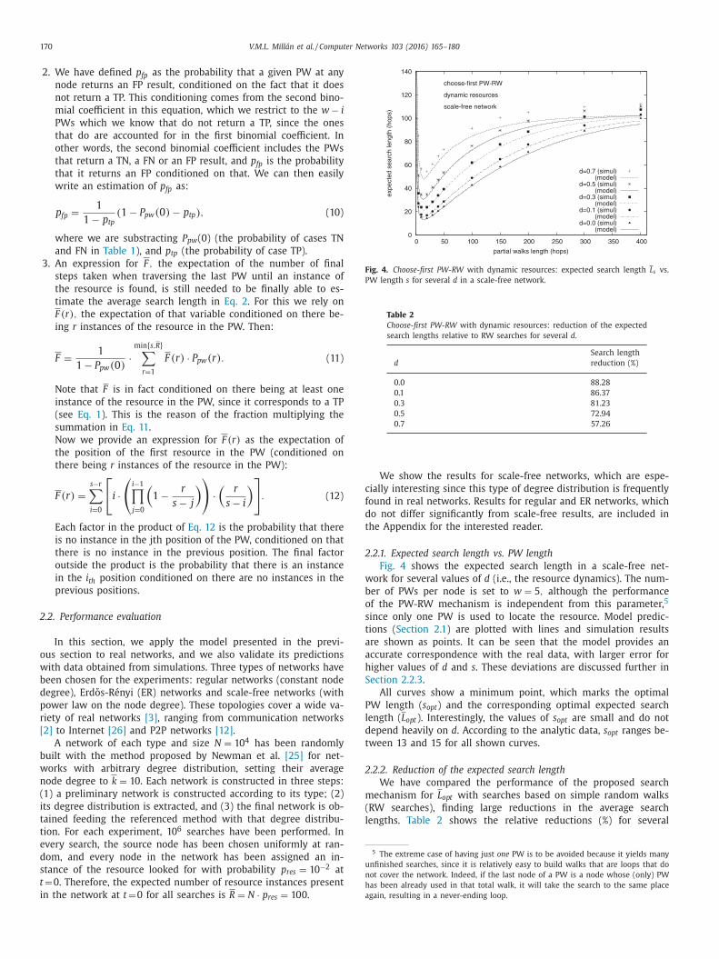
.2.1. Expected search length vs. PW length
Fig. 4 shows the expected search length in a scale-free net-
ork for several values of d (i.e., the resource dynamics). The num-
er of PWs per node is set to w = 5 , although the performance
f the PW-RW mechanism is independent from this parameter, 5
ince only one PW is used to locate the resource. Model predic-
ions ( Section 2.1 ) are plotted with lines and simulation results
re shown as points. It can be seen that the model provides an
ccurate correspondence with the real data, with larger error for
igher values of d and s . These deviations are discussed further in
ection 2.2.3 .
All curves show a minimum point, which marks the optimal
W length ( s opt ) and the corresponding optimal expected search
ength ( L opt ). Interestingly, the values of s opt are small and do not
epend heavily on d . According to the analytic data, s opt ranges be-
ween 13 and 15 for all shown curves.
.2.2. Reduction of the expected search length
We have compared the performance of the proposed search
echanism for L opt with searches based on simple random walks
RW searches), finding large reductions in the average search
engths. Table 2 shows the relative reductions (%) for several

V.M.L. Millán et al. / Computer Networks 103 (2016) 165–180 171
v
R
r
d
2
m
m
n
W
e
r
W
o
v
s
v
v
w
i
t
p
e
c
o
m
o
p
r
P
t
h
e
w
3
i
t
v
“
o
t
w
o
a
P
P
m
fi
s
r
r
t
fi
n
T
s
a
P
0
20
40
60
80
100
120
140
0 50 100 150 200 250 300 350 400
expe
cted
sea
rch
leng
th (
hops
)
partial walks length (hops)
check-first PW-RW
dynamic resources
scale-free network
w=5
d=0.7 (simul)(model)
d=0.5 (simul)(model)
d=0.3 (simul)(model)
d=0.1 (simul)(model)
d=0.0 (simul)(model)
Fig. 5. Check-first PW-RW ( w = 5 ) with dynamic resources: expected search length
L s vs. PW length s for several d in a scale-free network.
3
c
m
t
s
r
a
P
t
E
o
s
b
a
l
e
c
F
3
u
c
a
3
f
t
c
i
c
alues of d . We can see that the reductions that choose-first PW-
W achieves with respect to RW searches are lower for higher d ,
anging from around 88% in the case when d = 0 to 57% when
= 0.7.
.2.3. Deviations of the predictions of the analytical model
It can be concluded from Fig. 4 that the proposed analytical
odel succeeds in capturing the general behavior of the search
echanism observed in the simulations. There are, however, sig-
ificant deviations that deserve further evaluation and discussion.
e look first at the region of the graphic corresponding to inter-
sting practical scenarios, i.e., values of s close to s opt . For s = 20 ,
elative deviations range between 2.9% ( d = 0 . 0 ) and 7.9% ( d = 0 . 7 ).
e now look at the region for large s , to explore the dependency
f the deviation on the length of the PWs. For s = 300 , relative de-
iations are slightly larger, ranging between 3.6% and 8.2%.
These deviations may be explained by one aspect of the con-
truction of PWs that is not captured by our analytical model: re-
isits within a PW. That is, when constructing a PW, the next node
isited by the random walk can be one already in that PW. This
ill in general happen for several nodes of the PW, with increas-
ng probability for longer PWs (larger s ). Now consider a search
raversing a PW with revisited nodes. In the calculation of the
robability that a PW contains the resource, our analysis consid-
rs each node of the PW independent from the others, which is
learly not true for a revisited node (which appears more than
nce in the PW but is in fact the same node). This makes our
odel slightly optimistic because it overestimates the probability
f a PW containing the resource, and therefore underestimates the
robability of a query to that PW resulting in a false positive when
esources disappear. This means that there will actually be more
W traversals caused by false positives than expected, increasing
he average search length in simulations. This effect is larger for
igher d when more resources disappear and therefore more than
xpected PWs cause false positive queries, which is in accordance
ith Fig. 4 .
. Check-first PW-RW with dynamic resources
This section describes a variation of the mechanism presented
n Section 2 . Suppose the search is currently in a node and it needs
o pick one of the PWs in that node to decide whether to tra-
erse it or to jump over it. Recall from stage 2 under paragraph
The search mechanism” that the original mechanism first chooses
ne of the PWs at random, and then checks its associated informa-
ion for the desired resource, resembling the behavior of a random
alk. The proposed variation, on the other hand, reverses the order
f these tasks. It first checks the associated resource information of
ll the PWs of the node, and then randomly chooses among the
Ws with a positive result, if any (otherwise, it chooses among all
Ws of the node, as the original version). This check-first PW-RW
echanism improves the performance of the original (or choose-
rst PW-RW ) since the probability of choosing a PW with the re-
ource increases, with no extra storage space cost.
There is another, less important, difference between the algo-
ithms. In the original version, the nodes whose resources were
egistered in the information associated to the PW ranged between
he current node and the one before the last node. In the check-
rst version, the resource information is registered from the first
ode (the next to the current node) to the last node in the PW.
his change slightly improves the performance of the new version,
ince the probability of choosing a PW with the resource increases
lso in the cases where the resource is held by the last node of the
W. The rest of the operation of the mechanism remains the same.
.1. Analysis
Most of the analysis provided in Section 2.1 is still valid for
heck-first PW-RW . We present here the equations that need to be
odified to reflect the new behavior. That is the case of Eq. 3 for
he probabilities of choosing a PW with a TP, FP and negative re-
ult, respectively. Their counterparts follow. Remember that i and j
epresent the number of PWs of the node that return a TP result
nd an FP result, respectively:
P tp =
w ∑
i =1
w −i ∑
j=0
P (i, j) · i
i + j ,
fp =
w −1 ∑
i =0
w −i ∑
j=1
P (i, j) · j
i + j ,
P n = P (0 , 0) = 1 − P tp − P fp , (13)
The expression for the expectation of the number of final steps
aken when traversing the last PW until the resource is found (
q. 11 ) is still valid. It uses F (r) , the expectation of the position
f the first resource in the PW, conditioned on there being r in-
tances of the resource in the PW. Its expression ( Eq. 12 ) needs to
e modified, since the range of nodes whose resources are associ-
ted with the PW has changed from [0 , s − 1] to [1, s ]. The indexes
imits and their use in the expression have been updated as nec-
ssary in the new expression, which completes the analysis of the
heck-first PW-RW mechanism:
(r) =
s −r+1 ∑
i =1
[
i ·(
i −1 ∏
j=1
(1 − r
s − j + 1
))
·(
r
s − i + 1
)]
. (14)
.2. Performance evaluation
For the performance evaluation of the check-first PW-RW , we
se the same scenarios used in the performance evaluation of the
hoose-first PW-RW . As earlier, the corresponding figures for regular
nd ER networks can be found in the Appendix.
.2.1. Expected search length vs. PW length
Fig. 5 shows the expected search length in a scale-free network
or several values of d , and for w = 5 . The shape of the curves is
he same as that for the original mechanism ( Fig. 4 ), and the dis-
ussion on the observed deviations of the analytical results given
n Section 2.2.3 is also applicable to this case.
A substantial decrease in the optimal search length ( L opt ) for
heck-first PW-RW is observed. For example, for d = 0 . 3 , L opt is

172 V.M.L. Millán et al. / Computer Networks 103 (2016) 165–180
0
20
40
60
80
100
0 10 20 30 40 50 60
expe
cted
sea
rch
leng
th (
hops
)
partial walks length (hops)
choose-first / check-first PW-RW
dynamic resources
scale-free network
d=0.3
choose-first (simul)(model)
check-first, w=2 (simul)(model)
check-first, w=5 (simul)(model)
check-first, w=10 (simul)(model)
Fig. 6. PW-RW with dynamic resources: expected search length L s vs. PW length s
for choose-first PW-RW and check-first PW-RW ( w = 2 , 5 , 10 ) in a scale-free network
with d = 0 . 3 .
Table 3
Check-first PW-RW ( w = 5 ) with dynamic resources: reduc-
tion of the expected search lengths relative to RW searches
for several d .
Search length
d reduction (%)
0 .0 94 .29 %
0 .1 93 .44 %
0 .3 91 .04 %
0 .5 86 .91 %
0 .7 78 .68 %
4
s
w
n
a
o
t
p
a
(
P
s
b
l
n
i
n
p
s
i
m
W
W
e
t
t
t
i
4
d
n
L
E
t
v
i
w
8
a
o
r
F
w
t
t
F
b
F
6 New nodes with fresh resource instances will become useful from the searches
point of view when PWs are recomputed at t =T .
around 11, while it was about 21 for the choose-first PW-RW mech-
anism. The optimal PW length also diminishes, from about 14 to
6 in that case. The expected search length decrease is due to the
fact that the new mechanism checks all the PWs in the node for
the resource and then chooses one only among those with positive
result, increasing the probability of choosing a PW that currently
holds the resource. Following this reasoning, the more PWs in the
node, the higher this probability. It is therefore interesting to ex-
plore the dependency of L and s opt with w .
Fig. 6 shows the expected search length of the check-first PW-
RW mechanism, for w = 2 , 5 and 10 with d = 0 . 3 . To make the
comparison of performance between both mechanisms easier, a
curve corresponding to choose-first PW-RW has been added to the
graph. As explained above, the performance of the latter is inde-
pendent from w , but it plays a central role in the check-first PW-
RW . The range of the axes of this graph has been restricted to fo-
cus on the area around s opt . For higher s , the curves for the several
w converge. As expected, it is observed that higher w yields lower
L opt , with a value about 8 for w = 10 . Another interesting observa-
tion is that s opt also diminishes for higher w , falling to 4 in this
case.
These values mean a reduction of about 92% in the expected
search length of simple random walks, with 10 precomputed PWs
of just four nodes. Higher reductions can be achieved, at the ex-
pense of increasing the cost of the computation of the PWs, as an-
alyzed in Section 6 .
3.2.2. Reduction of the expected search length
Table 3 is provided as a reference, presenting the reduc-
tions achieved by check-first PW-RW with respect to random walk
searches for w = 5 and several d . We see that reductions range be-
tween 94% and 78%, while those of choose-first PW-RW ranged be-
tween 88% and 57%. That is an additional reduction of about 50%.
. Choose-first and check-first PW-RW with dynamic nodes
So far we have analyzed the performance of PW-RW when re-
ource instances dynamically appear in, and disappear from, net-
ork nodes. In this section, we explore the case where network
odes themselves leave and join the network. In our model, we
ssume that at time t =T , some nodes have left the network and
thers have joined it (recall that PWs were computed initially at
ime t =0 ). Nodes that have left the network have a double im-
act on PW-RW: (1) their resource instances are no longer avail-
ble, so the information on the resources in a PW is degraded, and
2) searches will not be able to visit them when following their
Ws. On the other hand, new nodes have no impact on PW-RW:
ince they are not in the previously computed PWs, they will not
e used by searches, even if they hold instances of the resource
ooked for. 6 Therefore, a single parameter l , the probability that a
ode present at t =0 has left at t =T , is enough to evaluate the
mpact on PW-RW performance at t =T . At this time, the expected
umber of resource instances is Np res (1 − l) , in a network with ex-
ected size N(1 − l) . This implies that the expected number of re-
ource instances per node is still p res , which allows a fair compar-
son with the baseline (static) case. The algorithm for the PW-RW
echanisms needs to be adapted for the dynamic nodes scenario.
e call nodes that remain in the network at t =T active nodes .
hen traversing a PW, the walk will visit the first active node at
ach hop. Similarly, when jumping over a PW, the walk will hop to
he last active node in the PW. If no active nodes remain in the PW,
he search will proceed visiting any active neighbor or will stop if
here are none (only searches that find the resource are included
n the performance evaluation results shown later).
.1. Analysis
The analytical models in Section 2 and 3 are modified for the
ynamic nodes scenario as follows. The expected length of a PW is
ow s (1 − l) . Therefore, Eq. 2 becomes:
s =
1
P tp · (P n + s (1 − l) · P fp ) + F . (15)
q. 3 for choose-first PW-RW are still valid, and so are their coun-
erpart Eq. 13 for check-first PW-RW . We need to provide a new
ersion of p tp in Eq. 4 , since the reason of information degradation
s now the dynamics of nodes:
p tp =
min { s, R } ∑
r=1
P pw
(r) · (1 − l r ) , (16)
ith P pw
( r ) given by the original Eq. 9 , which relied on Eqs. 7 and
. Eq. 10 for p fp can still be used, with the new definition of p tp
bove. Finally, a new expression for F is needed, since it depends
n the number of active nodes u in the last PW, which is now a
andom variable:
=
s ∑
u =1
F (u ) · P pw
(u ) , (17)
here F (u ) is the expected number of final steps conditioned on
here being u active nodes in the PW, and P pw
( u ) is the probability
hat the PW has u active nodes. To obtain the former we rely on
(u, r) , the expected number of final steps conditioned on there
eing r instances of the resource in a PW with u active nodes:
(u ) =
1
1 − P pw
(u, 0) ·
min { u, R } ∑
r=1
F (u, r) · P pw
(u, r) , (18)

V.M.L. Millán et al. / Computer Networks 103 (2016) 165–180 173
0
20
40
60
80
100
120
140
0 50 100 150 200 250 300 350 400
expe
cted
sea
rch
leng
th (
hops
)
partial walks length (hops)
choose-first PW-RW
dynamic nodes
scale-free network
l=0.7 (simul)(model)
l=0.5 (simul)(model)
l=0.3 (simul)(model)
l=0.1 (simul)(model)
l=0.0 (simul)(model)
Fig. 7. Choose-first PW-RW with dynamic nodes: expected search length L s vs. PW
length s for several l in a scale-free network.
w
i
b
F
T
P
w
i
L
P
w
4
n
d
u
4
w
n
t
s
S
r
i
(
a
c
s
P
o
f
t
Table 4
Choose-first PW-RW with dynamic nodes: reduction of the
expected search lengths relative to RW searches for several
l .
Search length
d reduction (%)
0 .0 88 .28 %
0 .1 87 .08 %
0 .3 84 .21 %
0 .5 80 .21 %
0 .7 73 .58 %
0
20
40
60
80
100
120
140
0 50 100 150 200 250 300 350 400ex
pect
ed s
earc
h le
ngth
(ho
ps)
partial walks length (hops)
check-first PW-RW
dynamic nodes
scale-free network
w=5
l=0.7 (simul)(model)
l=0.5 (simul)(model)
l=0.3 (simul)(model)
l=0.1 (simul)(model)
l=0.0 (simul)(model)
Fig. 8. Check-first PW-RW ( w = 5 ) with dynamic nodes: expected search length L s vs. PW length s for several l in a scale-free network.
0
20
40
60
80
100
0 10 20 30 40 50 60
expe
cted
sea
rch
leng
th (
hops
)
partial walks length (hops)
choose-first / check-first PW-RW
dynamic nodes
scale-free network
l=0.3
choose-first (simul)(model)
check-first, w=2 (simul)(model)
check-first, w=5 (simul)(model)
check-first, w=10 (simul)(model)
Fig. 9. PW-RW with dynamic nodes: expected search length L s vs. PW length s
for choose-first PW-RW and check-first PW-RW ( w = 2 , 5 , 10 ) in a scale-free network
with d = 0 . 3 .
a
f
c
7
t
l
t
i
r
t
a
fi
(
r
here P pw
( u, r ) is the probability of a PW with u active nodes hav-
ng r instances of the resource. Now, an estimation for F (u, r) can
e obtained reasoning as for Eq. 12 :
(u, r) =
u −r ∑
i =0
[
i ·(
i −1 ∏
j=0
(1 − r
u − j
))
·(
r
u − i
)]
. (19)
he expression for P pw
( u ) can be obtained as in Eq. 9 :
pw
(u ) =
(s u
)· (p rw,a )
u · (1 − p rw,a ) s −u , (20)
here p rw, a , the probability that a node visited by a RW is active,
s:
p rw,a =
N(1 − l) · k
S − k rw
. (21)
ikewise, the expression for P pw
( u, r ) is:
pw
(u, r) =
(u
r
)· (p rw
) r · (1 − p rw
) u −r , (22)
here p rw
is given by Eq. 7 .
.2. Performance evaluation
We look now at the performance of the PW-RW mechanisms in
etworks with dynamic nodes, that operate according to the model
escribed in the previous section. As earlier, the corresponding fig-
res for regular and ER networks can be found in the Appendix.
.2.1. Expected search length vs. PW length
Fig. 7 shows results for choose-first PW-RW in a scale-free net-
ork for several values of l , the probability of a node leaving the
etwork. Predictions of the analytical model in Section 4 , plot-
ed as lines, provide accurate estimations for experimental re-
ults, shown as points. The observed deviations are discussed in
ection 4.2.3 .
The effect of node dynamics is in general very similar to that of
esource dynamics (see Fig. 4 ). We note, however, that s opt slightly
ncreases with l in Fig. 7 , while it slightly decreased for larger d
the probability of a resource instance disappearing) in Fig. 4 . In
ddition, we see that L opt remains lower in the dynamic nodes
ase as l grows, compared to the dynamic resources case for the
ame values of d . Both effects have their origin in the fact that
Ws are effectively shorter in the dynamic nodes case, since some
f their nodes are no longer in the network when searches are per-
ormed. This contributes to shorten the searches, obtaining the op-
imal lengths with originally longer PWs.
Table 4 shows the reductions in expected search length
chieved by choose-first PW-RW relative to RW searches in scale-
ree networks with dynamic nodes. As for the dynamic resources
ase ( Table 2 ), reductions are similar, ranging in this case between
3% and 88%. Reductions for large l are significantly higher than
hose for large d in the dynamic resources case (about 73% for
= 0 . 7 vs. about 57% for d = 0 . 7 ). This is explained as above by
he effectively shorter PWs in the dynamic nodes case.
Fig. 8 shows the results for the check-first PW-RW mechanism
n a scale-free network with dynamic nodes. As in the dynamic
esources case (see Fig. 5 ), both s opt and L opt decrease with respect
o the choose-first mechanism, since the algorithm checks all PWs
vailable at the node for the resource, increasing the probability of
nding it. Fig. 9 shows that both L opt and s opt decrease for larger w
the number of PWs per node), as observed also for the dynamic
esources case (see Fig. 6 ).

174 V.M.L. Millán et al. / Computer Networks 103 (2016) 165–180
Table 5
Check-first PW-RW ( w = 5 ) with dynamic nodes: reduction
of the expected search lengths relative to RW searches for
several l .
Search length
d reduction (%)
0 .0 94 .29 %
0 .1 93 .76 %
0 .3 92 .48 %
0 .5 90 .68 %
0 .7 87 .73 %
0
20
40
60
80
100
120
0 0.5 1 1.5 2
expe
cted
sea
rch
leng
th (
hops
)
c (perturbation of pres)
dynamic resources (d = 0.3)
scale-free network
pres = c * (baseline pres)
baseline pres = 0.01
choose-first PW-RW (fixed s) (adaptive s)
check-first PW-RW (fixed s) (adaptive s)
Fig. 10. PW-RW with dynamic resources: expected search length L s vs. c , the per-
turbation of p res in a scale-free network with d = 0 . 3 .
u
P
p
l
l
s
i
t
s
R
m
a
n
a
a
a
i
a
v
b
6
s
P
t
t
s
i
v
t
P
T
a
i
l
o
a
c
m
f
a
n
4.2.2. Reduction of the expected search length
Finally, Table 5 shows the reductions in expected search length
of check-first PW-RW compared to RW searches. Reduction values
range between 87% and 94%. Again, reductions for high l are larger
than in the dynamic resources case for large d (around 87% for l =0 . 7 vs. 77% for d = 0 . 7 ). Reductions relative to choose-first PW-RW
are above 51%, slightly larger than for the dynamic resource case.
4.2.3. Deviations of the predictions of the analytical model
Figs. 7 and 8 show deviations of the proposed analytical model
with respect to simulation results. These deviations are very sim-
ilar to those for the dynamic resources scenario, discussed in
Section 2.2.3 . For example, deviations of the analytical model for
choose-first PW-RW with dynamic nodes range from 3.2% ( l = 0 . 0 )
to 9.4% ( l = 0 . 7 ) when s = 20 , and from 3.7% to 10.3% when s =300 . As for the dynamic resources case, these deviations may be
caused by revisits within PWs. Our analytical models do not take
this effect into account, resulting in optimistic predictions (see
Section 2.2.3 ).
5. Robustness of PW-RW to parameter perturbations
In this section, we assess the robustness of the proposed mech-
anisms to variations of some of the parameters, relative both to the
network and to the mechanisms themselves. For this, we use the
analytical models defined and validated against simulation results
in the previous sections. The PW-RW mechanisms have two pa-
rameters: the length of the PWs ( s ) and the number of PWs per
node ( w ). The impact of variations of s on the expected search
length has already been shown in Figs. 4 to 9 , revealing the exis-
tence of an optimal length for PWs ( s opt ), which achieves minimum
expected search length. As for w , it is only relevant for check-first
PW-RW , since all the PWs available in the node are checked for the
resource. Figs. 6 and 9 show that the minimum expected search
length (and also s opt ) decreases as w is increased, as expected.
Regarding network parameters, we have already studied the im-
pact of the dynamics of resources (through d , the probability that
a resource disappears from a node) and of the dynamics of nodes
(through l , the probability that a node leaves the network), observ-
ing that the minimum expected search lengths remain reasonably
low even for high volatility probabilities (see Figs. 4 to 9 ).
We now investigate the effect of p res , the probability that a
node has an instance of the resource looked for, which in turn
determines the average number of instances in the network. We
write p res as a function of a multiplicative perturbation factor c
for the chosen baseline value (0.01), i.e., p res = 0 . 01 · c. Then we
vary c in the range [0.1, 2] and observe the performance of the
mechamisms in a scale-free network with dynamic resources ( d =0 . 3 ). We have found that the value of s opt itself varies when p res is
perturbed, ranging from 44 to 10 for choose-first and from 19 to 4
for check-first . We are presented with two options here: calculate
the expected search lengths with s fixed to the s opt correspond-
ing to the baseline p res (14 for choose-first and 6 for check-first ), or
se the actual s opt for each value of p res (in a hypothetical adaptive
W-RW). Fig. 10 compares both cases for choose-first PW-RW (up-
er curves) and check-first PW-RW (lower curves). Expected search
engths grow for c < 1 (as the number of resources decreases be-
ow the baseline), and diminish for c > 1 (as the number of re-
ources increases over the baseline), as expected. More interest-
ng is the fact that the proposed mechanisms (with fixed s ) and
he hypothetical adaptive versions achieve very similar expected
earch lengths in a wide range of c . This suggests that the PW-
W mechanisms are robust to variations of p res , with little perfor-
ance degradation due to the suboptimality of s when p res varies
round a baseline value. Results are similar for networks with dy-
amic nodes, and are not shown here.
Finally, we have checked that the expected search lengths (and
lso s opt ) do not depend on the network size ( N ), as long as p res
nd the average degree of the network remain unchanged. This is
s expected, since fixing p res means that the number of resource
nstances is proportional to the network size, and fixing the aver-
ge degree means that the number of choices of a random walk to
isit any endpoint in the network (the expected number of neigh-
ors of the current node) remains the same.
. Cost of the PW-RW mechanisms
In our proposed searching mechanisms, we assumed that at
ome initial time all network nodes compute a number w of
Ws that are used for an interval of time of length T . After that,
he searches performed in this interval use these PWs, and thus
he cost of their computation must be added to the cost of the
earches themselves. In this section we show that such an increase
s not relevant in the average cost per search, regardless of the
alue of T .
First, we observe that since the information associated with
hose initial PWs is degraded due to the network dynamics, new
Ws are computed at t =T to capture the current network state.
hese new PWs are then used for another interval of length T ,
nd so on. The election of the length of the PW recomputation
nterval T influences the total cost with two opposite effects. For
onger intervals, more searches share the cost of the computation
f PWs, lowering the cost per search. However, the information
ssociated with the PWs gets more degraded for longer intervals,
ausing longer searches. This suggests the existence of some opti-
al T opt that minimizes the total cost per search.
To investigate this we use C t , the average total cost per search
or interval length T , as defined in [17] for the static network case,
s the goodness metric to optimize. This total cost, defined as the
umber of messages, takes into account the cost of the average

V.M.L. Millán et al. / Computer Networks 103 (2016) 165–180 175
0
10
20
30
40
50
60
0 5 10 15 20 25 30
incr
emen
t of e
xpec
ted
sear
ch le
ngth
(%
)
resources that disappear (%)
choose-first / check-first PW-RW
dynamic resources
scale-free network
choose-firstcheck-first
0 5 10 15 20 25 30
nodes that leave (%)
choose-first / check-first PW-RW
dynamic nodes
scale-free network
choose-firstcheck-first
Fig. 11. Choose-first and check-first PW-RW in dynamic networks: relative increment
of the expected search length L s vs. (left) the fraction d of resource instances d that
disappear, and (right) the fraction l of nodes that leave the network, in a scale-free
network.
s
o
p
p
C
i
a
t
t
o
T
C
g
n
n
p
a
F
a
s
t
c
i
p
fi
a
w
l
c
w
p
t
n
I
t
d
d
w
0
10
20
30
40
50
60
0 200 400 600 800 1000
aver
age
tota
l cos
t per
sea
rch
(num
ber
of m
essa
ges)
length of recomputation interval (s)
choose-first / check-first PW-RW
dynamic resources
scale-free network
Dots mark the minimumvalue of each curve.
choose-first: μ = 5.0, λ = 0.05μ = 15.0, λ = 0.05
μ = 5.0, λ = 0.15check-first: μ = 5.0, λ = 0.05
μ = 15.0, λ = 0.05μ = 5.0, λ = 0.15
Fig. 12. Choose-first and check-first PW-RW with dynamic resources: average total
cost per search C t vs. the length of the PW recomputation interval T , in a scale-free
network.
0
10
20
30
40
50
60
0 200 400 600 800 1000
aver
age
tota
l cos
t per
sea
rch
(num
ber
of m
essa
ges)
length of recomputation interval (s)
choose-first / check-first PW-RW
dynamic nodes
scale-free network
Dots mark the minimumvalue of each curve.
choose-first: μ = 5.0, λ = 0.05μ = 15.0, λ = 0.05
μ = 5.0, λ = 0.15check-first: μ = 5.0, λ = 0.05
μ = 15.0, λ = 0.05μ = 5.0, λ = 0.15
Fig. 13. Choose-first and check-first PW-RW with dynamic nodes: average total cost
per search C t vs. the length of the PW recomputation interval T , in a scale-free
network.
r
t
s
t
C
t
t
T
C
w
t
h
a
c
i
o
l
b
F
earch ( L s messages plus one to notify the source) and the cost
f the computation of each of the w PWs of a node ( s messages
lus one to notify the node), divided by the number of searches b
erformed per node in the interval:
t = ( L s + 1) +
w
b (s + 1) . (23)
In dynamic networks, however, L s varies with time during the
nterval as information progressively degrades, so it needs to be
veraged over T . In addition, since we intend to study the average
otal cost as a function of T , the number of searches per node in
he interval depends on T as b = λT , if we assume that the number
f searches per node per time unit is a constant that we denote λ.
he previous equation then becomes:
t (T ) =
1
T
∫ T
0
( L s (t) + 1) · dt +
w
λT (s + 1) . (24)
L s (t) is determined by the stochastic process of deaths that is
overned by μk , the rate of departures of resource instances or
odes when the system is in state k (the number of instances or
odes). A rigorous approach to this problem would require a com-
lete stochastic characterization of the behavior of a system with
large number of states, and is out of the scope of this work.
or our purpose, we will focus on intervals of length T in which
relatively small fraction of resources or nodes leave the system,
o that the expected search length does not overly increase. For
hese intervals, we will assume that μ remains constant. This is
learly just an approximation to the behavior of a real system, but
t greatly simplifies the analysis allowing us to draw interesting
ractical conclusions.
To obtain an estimation of L s (t) under these assumptions, we
rst seek L s (d) , the relation between the expected search length
nd the fraction d of resource instances that disappear. Similarly,
e need to find L s (l) for networks with dynamic nodes. The fol-
owing discussion focuses on the dynamic resources case for con-
iseness. To find L s (d) , which we note is independent from time,
e use the analysis of the PW-RW mechanisms presented in the
revious sections.
Fig. 11 shows the increments in the expected search length for
he choose-first and check-first PW-RW mechanisms in a scale-free
etwork with dynamic resources (left) and dynamic nodes (right).
ncrements are obtained relative to the expected search length for
he static case (e.g., ( L s (d) − L s (0)) / L s (0) ). We observe that these
ependencies are approximately linear, with a slope α ≈ 2 for
ynamic resources and α ≈ 1 for dynamic nodes. We can then
rite L s (t) ≈ L s (0)(1 + αd(t)) . Now, if μ is the departure rate of
esource instances (or nodes), and assuming it constant for the in-
ervals of interest, we obtain an estimation for the fraction of in-
tances that have disappeared at time t as d ( t ) ≈ μt / N . With all
he above we can rewrite Eq. 24 as:
t (T ) =
1
T
∫ T
0
(L s (0) · (1 + α
μ
N
t) + 1
)· dt +
w
λT (s + 1)
=
(L s (0) + 1
)+
L s (0) · αμ
2 N
T +
w (s + 1)
λ
1
T . (25)
A simple calculation on the previous equation allows us to ob-
ain an expression for the interval T opt that minimizes the average
otal cost per search:
opt =
√
2 Nw (s + 1)
L s (0) · αμλ. (26)
Figs. 12 and 13 show plots of the average total cost per search
t ( T ) for the choose-first and check-first PW-RW mechanisms in net-
orks with dynamic resources and with dynamic nodes, respec-
ively, for several values of μ and λ. All curves have a linear be-
avior for large T (where cost is dominated by longer searches),
nd a rapid increase for small T (where cost is dominated by PW
omputation). The minimum cost, marked with a dot, can be found
n the region in between. Interestingly, this intermediate region is
bserved to be quite flat, which allows to reduce the interval T be-
ow T opt with no relevant increase in the average cost per search,
ut with significant reductions in the expected search length (see
ig. 11 ). This also means that the PW-RW mechanisms are not very

176 V.M.L. Millán et al. / Computer Networks 103 (2016) 165–180
0
20
40
60
80
100
120
140
0 50 100 150 200 250 300 350 400ex
pect
ed s
earc
h le
ngth
(ho
ps)
partial walks length (hops)
choose-first PW-RW
dynamic resources
regular network
d=0.7 (simul)(model)
d=0.5 (simul)(model)
d=0.3 (simul)(model)
d=0.1 (simul)(model)
d=0.0 (simul)(model)
Fig. A.14. Choose-first PW-RW with dynamic resources: expected search length L s vs. PW length s for several d in a regular network.
0
20
40
60
80
100
120
140
0 50 100 150 200 250 300 350 400
expe
cted
sea
rch
leng
th (
hops
)
partial walks length (hops)
choose-first PW-RW
dynamic resources
ER network
d=0.7 (simul)(model)
d=0.5 (simul)(model)
d=0.3 (simul)(model)
d=0.1 (simul)(model)
d=0.0 (simul)(model)
Fig. A.15. Choose-first PW-RW with dynamic resources: expected search length L s vs. PW length s for several d in a ER network.
0
10000
20000
30000
40000
50000
60000
0 20 40 60 80 100 120
abso
lute
freq
uenc
y
search length (hops)
choose-first PW-RWdynamic resourcesregular network
PW-RW d=0.0PW-RW d=0.1PW-RW d=0.3PW-RW d=0.5PW-RW d=0.7
RW
Fig. A.16. Choose-first PW-RW with dynamic resources: search length distributions
for RW searches and for PW-RW searches, in a regular network with s = 10 and
several d .
sensitive to the election of the length T of the recomputation in-
terval, given that the system remains in the intermediate region.
Finally, the plots of C t ( T ) also show that the cost increases for
more volatile networks (higher μ) and decreases for more frequent
searches (higher λ), as it was expected.
7. Conclusions
We have proposed a mechanism to locate a desired resource
in randomly built networks with dynamic resource behavior (re-
source instances can appear and disappear) or dynamic node be-
havior (nodes can join and leave the network). The mechanism is
based on building a total walk with partial walks that are precom-
puted as random walks and available at each network node. When
precomputing each partial walk, information on the resources held
by its nodes is stored and associated to it. This information is used
by the searches, so that they can jump over partial walks in which
the desired resource is not located. Two versions of the mechanism
have been described. In the choose-first version, one of the partial
walks at the current node is randomly chosen, and then checked
for the desired resource. In the check-first version, all the partial
walks of the node are checked for the resource, and then one is
randomly chosen among those in which the resource was found.
We have presented an analytical model that predicts the expected
search length achieved by the two versions of the mechanism. Sim-
ulation experiments have been used to validate the model and to
assess the effect of resource and node dynamics. We have found
that the choose-first version achieves large reductions of the aver-
age search length in relation to searches based on simple random
walks. These reductions remain significant even in the face of high
volatility of resources or nodes. The check-first version produces
larger reductions as we increase the number of partial walks pre-
computed at each node (at the corresponding extra cost). Results
have been found to be very similar for networks with different
degree distributions ( k -regular, Erd ̋os-Rényi and scale-free). Finally,
we have analyzed the cost of the PW-RW mechanisms, concluding
that the choice of the length of the PW precomputation interval
does not have a significant impact on the cost in a wide range of
interval lengths.
An interesting future work line for this study is to measure the
improvement in the search length that can be obtained by using
different strategies to choose one of the partial walks available in
a node. Another possibility to shorten search lengths is to use more
intelligent (and more costly) variations of random walks instead of
simple random walks.
Appendix A. Choose-first PW-RW with dynamic resources
This Appendix contains results for regular and ER networks that
complement those given for scale-free networks in the main text,
as well as some additional results. Results for the three network
types are very similar in all cases.
Figs. A.14 and A.15 show experimental and analytical results
for the expected search length achieved by choose-first PW-RW in
regular and ER networks with dynamic resources, respectively, for
several values of p , the probability of a resource disappearing from
a node.
• Length distributions and dispersion:
The use of partial walks also affects the shape of the proba-
bilistic distribution of search lengths. Figs. A .16 and A .17 show
the distributions for simple random walks (RW) searches and
for PW-RW searches, for s = 10 and for several values of d ,
obtained from the experiments with regular and ER networks
with dynamic resources. Instead of the slowly decaying distri-
bution of RWs, the proposed mechanism exhibits search length
distributions that show a maximum frequency for a small
search length and then decay much faster than the random
walk distribution. We also note that the search length for the
maximum frequency (9 in this case) is independent from the
dynamic behaviour of resources ( d ). The search length distribu-
tions of PW-RW have therefore lower standard deviation than
random walk searches. For d = 0 . 3 , for instance, the standard
deviation in regular, ER and scale-free networks are, respec-
tively, 21.06, 21.34 and 21.58. Correspondingly, the mean search
lengths are 23.56, 23.72 and 23.81. As a reference for compari-
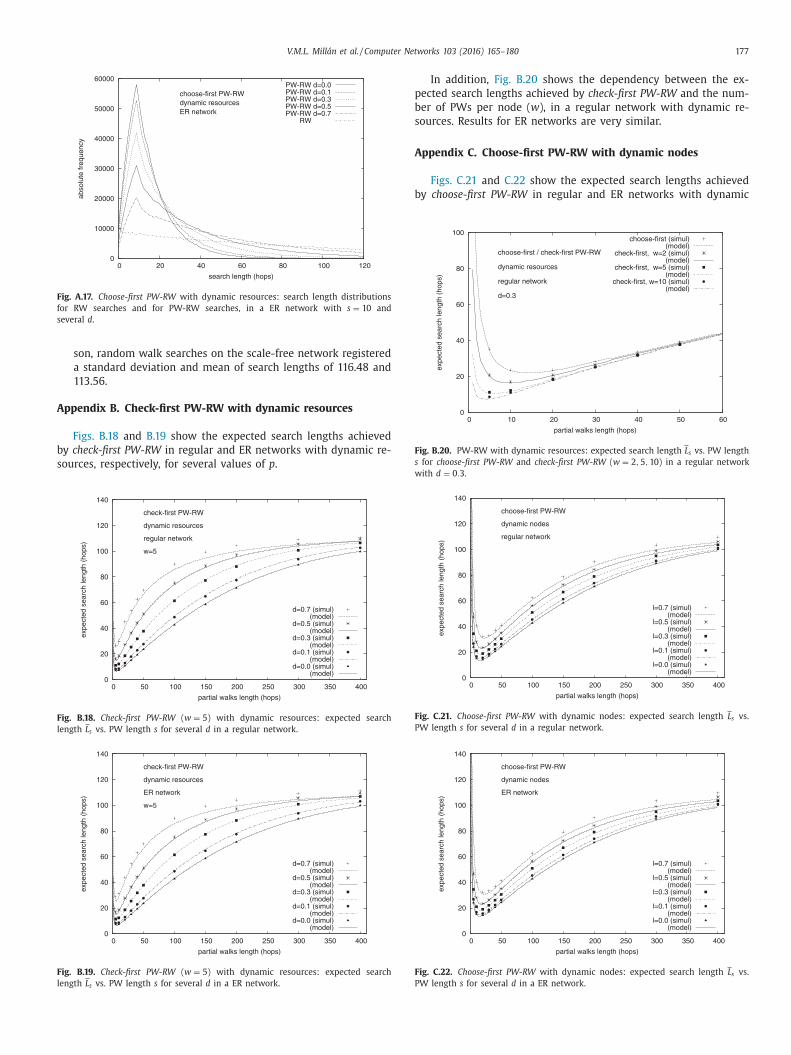
V.M.L. Millán et al. / Computer Networks 103 (2016) 165–180 177
0
10000
20000
30000
40000
50000
60000
0 20 40 60 80 100 120
abso
lute
freq
uenc
y
search length (hops)
choose-first PW-RWdynamic resourcesER network
PW-RW d=0.0PW-RW d=0.1PW-RW d=0.3PW-RW d=0.5PW-RW d=0.7
RW
Fig. A.17. Choose-first PW-RW with dynamic resources: search length distributions
for RW searches and for PW-RW searches, in a ER network with s = 10 and
several d .
A
b
s
F
l
F
l
p
b
s
A
b
0
20
40
60
80
100
0 10 20 30 40 50 60
expe
cted
sea
rch
leng
th (
hops
)partial walks length (hops)
choose-first / check-first PW-RW
dynamic resources
regular network
d=0.3
choose-first (simul)(model)
check-first, w=2 (simul)(model)
check-first, w=5 (simul)(model)
check-first, w=10 (simul)(model)
Fig. B.20. PW-RW with dynamic resources: expected search length L s vs. PW length
s for choose-first PW-RW and check-first PW-RW ( w = 2 , 5 , 10 ) in a regular network
son, random walk searches on the scale-free network registered
a standard deviation and mean of search lengths of 116.48 and
113.56.
ppendix B. Check-first PW-RW with dynamic resources
Figs. B.18 and B.19 show the expected search lengths achieved
y check-first PW-RW in regular and ER networks with dynamic re-
ources, respectively, for several values of p .
0
20
40
60
80
100
120
140
0 50 100 150 200 250 300 350 400
expe
cted
sea
rch
leng
th (
hops
)
partial walks length (hops)
check-first PW-RW
dynamic resources
regular network
w=5
d=0.7 (simul)(model)
d=0.5 (simul)(model)
d=0.3 (simul)(model)
d=0.1 (simul)(model)
d=0.0 (simul)(model)
ig. B.18. Check-first PW-RW ( w = 5 ) with dynamic resources: expected search
ength L s vs. PW length s for several d in a regular network.
0
20
40
60
80
100
120
140
0 50 100 150 200 250 300 350 400
expe
cted
sea
rch
leng
th (
hops
)
partial walks length (hops)
check-first PW-RW
dynamic resources
ER network
w=5
d=0.7 (simul)(model)
d=0.5 (simul)(model)
d=0.3 (simul)(model)
d=0.1 (simul)(model)
d=0.0 (simul)(model)
ig. B.19. Check-first PW-RW ( w = 5 ) with dynamic resources: expected search
ength L s vs. PW length s for several d in a ER network.
w
F
P
F
P
In addition, Fig. B.20 shows the dependency between the ex-
ected search lengths achieved by check-first PW-RW and the num-
er of PWs per node ( w ), in a regular network with dynamic re-
ources. Results for ER networks are very similar.
ppendix C. Choose-first PW-RW with dynamic nodes
Figs. C.21 and C.22 show the expected search lengths achieved
y choose-first PW-RW in regular and ER networks with dynamic
ith d = 0 . 3 .
0
20
40
60
80
100
120
140
0 50 100 150 200 250 300 350 400
expe
cted
sea
rch
leng
th (
hops
)
partial walks length (hops)
choose-first PW-RW
dynamic nodes
regular network
l=0.7 (simul)(model)
l=0.5 (simul)(model)
l=0.3 (simul)(model)
l=0.1 (simul)(model)
l=0.0 (simul)(model)
ig. C.21. Choose-first PW-RW with dynamic nodes: expected search length L s vs.
W length s for several d in a regular network.
0
20
40
60
80
100
120
140
0 50 100 150 200 250 300 350 400
expe
cted
sea
rch
leng
th (
hops
)
partial walks length (hops)
choose-first PW-RW
dynamic nodes
ER network
l=0.7 (simul)(model)
l=0.5 (simul)(model)
l=0.3 (simul)(model)
l=0.1 (simul)(model)
l=0.0 (simul)(model)
ig. C.22. Choose-first PW-RW with dynamic nodes: expected search length L s vs.
W length s for several d in a ER network.

178 V.M.L. Millán et al. / Computer Networks 103 (2016) 165–180
s
P
s
R
nodes, respectively, for several values of l , the probability of a node
leaving the network.
Appendix D. Check-first PW-RW with dynamic nodes
Figs. D.23 and D.24 show the expected search lengths achieved
by check-first PW-RW in regular and ER networks with dynamic
nodes, respectively, for several values of l .
0
20
40
60
80
100
120
140
0 50 100 150 200 250 300 350 400
expe
cted
sea
rch
leng
th (
hops
)
partial walks length (hops)
check-first PW-RW
dynamic nodes
regular network
w=5
l=0.7 (simul)(model)
l=0.5 (simul)(model)
l=0.3 (simul)(model)
l=0.1 (simul)(model)
l=0.0 (simul)(model)
Fig. D.23. Check-first PW-RW ( w = 5 ) with dynamic nodes: expected search length
L s vs. PW length s for several d in a regular network.
0
20
40
60
80
100
120
140
0 50 100 150 200 250 300 350 400
expe
cted
sea
rch
leng
th (
hops
)
partial walks length (hops)
check-first PW-RW
dynamic nodes
ER network
w=5
l=0.7 (simul)(model)
l=0.5 (simul)(model)
l=0.3 (simul)(model)
l=0.1 (simul)(model)
l=0.0 (simul)(model)
Fig. D.24. Check-first PW-RW ( w = 5 ) with dynamic nodes: expected search length
L s vs. PW length s for several d in a ER network.
0
20
40
60
80
100
0 10 20 30 40 50 60
expe
cted
sea
rch
leng
th (
hops
)
partial walks length (hops)
choose-first / check-first PW-RW
dynamic nodes
regular network
l=0.3
choose-first (simul)(model)
check-first, w=2 (simul)(model)
check-first, w=5 (simul)(model)
check-first, w=10 (simul)(model)
Fig. D.25. PW-RW with dynamic nodes: expected search length L s vs. PW length
s for choose-first PW-RW and check-first PW-RW ( w = 2 , 5 , 10 ) in a regular network
with d = 0 . 3 .
[
[
[
[
Finally, Fig. D.25 shows the dependency between the expected
earch lengths achieved by check-first PW-RW and the number of
Ws per node ( w ), in a regular network with dynamic nodes. Re-
ults for ER networks are very similar.
eferences
[1] L.A. Adamic , R.M. Lukose , A.R. Puniyani , B.A. Huberman , Search in power-lawnetworks, Phys. Rev. E. 64 (046135) (2001) .
[2] W. Aiello, F. Chung, L. Lu, A random graph model for massive graphs, in: Pro-ceedings of the Thirty-second Annual ACM Symposium on Theory of Comput-
ing, in: STOC ’00, ACM, New York, NY, USA, 20 0 0, pp. 171–180, doi: 10.1145/
335305.335326 . [3] R. Albert, A.-L. Barabási, Statistical mechanics of complex networks, Rev. Mod.
Phys. 74 (1) (2002) 47–97, doi: 10.1103/RevModPhys.74.47 . [4] D. Amit , G. Parisi , L. Peliti , Asymptotic behavior of the ‘true’ self-avoiding walk,
Phys. Rev. B. 27 (1983) 1635–1645 . [5] Y. Chawathe , S. Ratnasamy , N. Lanham , S. Shenker , Making gnutella-like
p2psystems scalable, in: Proceedings of the 2003 Conference on Applications,
Technologies, Architectures, and Protocols for Computer Communications (SIG-COMM)Karlsruhe, Germany, 2003, pp. 407–418 .
[6] L. da Fontoura Costa , G. Travieso , Exploring complex networks through randomwalks, Phys. Rev. E. 75 (016102) (2007) .
[7] A. Das Sarma, D. Nanongkai, G. Pandurangan, P. Tetali, Efficient distributed ran-dom walks with applications, in: Proceeding of the 29th ACM SIGACT-SIGOPS
symposium on Principles of distributed computing, in: PODC ’10, ACM, New
York, USA, 2010, pp. 201–210. http://doi.acm.org/10.1145/1835698.1835745 . [8] S. Dolev , E. Schiller , J.L. Welch , Random walk for self-stabilizing group commu-
nication in ad hoc networks, IEEE Trans. Mobile Comput. 5 (7) (2006) 893–905 .[9] S. Fortunato , A. Flammini , Random walks on directed networks: the case of
pagerank, e-print physics (0604203) (2006) . [10] C. Gkantsidis , M. Mihail , A. Saberi , Random-walks in peer-to-peer networks:
algorithms and evaluation, Perform. Eval. 63 (2006) 241–263 . [11] B.D. Hughes , Random walks and random environments, vol. 1, Clarendon Press,
Oxford, 1995 .
[12] M.A. Jovanovic , Modeling large-scale peer-to-peer networks and a case studyof gnutella, University of Cincinatti, Cincinatti, Ohio, 2001 Master’s thesis .
[13] M.A. Jovanovic , F.S. Annexstein , K.A. Berman , Scalability issues in large peer–to-peer networks - a case study of Gnutella, Technical Report, Technical report,
University of Cincinnati, 2001 . [14] B. Krishnamurthy, J. Wang, Y. Xie, Early measurements of a cluster-based archi-
tecture for p2p systems, in: Proceedings of the 1st ACM SIGCOMM Workshop
on Internet Measurement, in: IMW ’01, ACM, New York, USA, 2001, pp. 105–109, doi: 10.1145/505202.505216 .
[15] C. Law , K.-Y. Siu , Distributed construction of random expander networks, in:Proceedings of the Twenty-second Annual Joint Conference of the IEEE Com-
puter and Communications Societies (INFOCOM 2003), 3, 2003, pp. 2133–2143 .[16] S.H. Lee , P.-J. Kim , H. Jeong , Statistical properties of sampled networks, Phys.
Rev. E. 73 (016102) (2006) .
[17] V. López Millán, V. Cholvi, A. Fernández Anta, L. López, Improve resource loca-tion with locally precomputed partial random walks, Computing 97 (9) (2015)
871–891, doi: 10.10 07/s0 0607- 013- 0353- x . [18] L. Lovász , Random walks on graphs: a survey, in: Combinatorics, Paul Erd ̋os is
eighty, vol. 2, Keszthely, Hungary, 1993, pp. 1–46 . [19] Q. Lv, P. Cao, E. Cohen, K. Li, S. Shenker, Search and replication in unstruc-
tured peer-to-peer networks, in: ICS ’02: Proceedings of the 16th Interna-
tional Conference on Supercomputing, ACM, New York, USA, 2002, pp. 84–95.http://doi.acm.org/10.1145/514191.514206 .
[20] Q. Lv , S. Ratnasamy , S. Shenker , Can heterogeneity make gnutella scalable? in:Revised papers from the First International Workshop on Peer-to-Peer Systems,
Cambridge, United States, 2002, pp. 94–103 . [21] I. Mabrouki , X. Lagrange , G. Froc , Random walk based routing protocol for
wireless sensor networks, in: Proceedings of the Second International Con-
ference on Performance Evaluation Methodologies and Tooks (ValueTools ’07),ICST (Institute for Computer Sciences, Social-Informatics and Telecommunica-
tions Engineering), 2007, pp. 1–10 . 22] G.S. Manku, M. Naor, U. Wieder, Know thy neighbor’s neighbor: The power
of lookahead in randomized p2p networks, in: Proceedings of the Thirty-sixthAnnual ACM Symposium on Theory of Computing, in: STOC ’04, ACM, New
York, NY, USA, 2004, pp. 54–63, doi: 10.1145/1007352.1007368 .
23] P. Maymounkov , D. Mazières , Kademlia: A peer-to-peer information systembased on the xor metric, in: Revised Papers from the First International Work-
shop on Peer-to-Peer Systems, in: IPTPS ’01, Springer-Verlag, London, UK, 2002,pp. 53–65 .
[24] M.E.J. Newman , A.-L. Barabási , D.J. Watts , The Structure and Dynamics of Net-works, Princeton University Press, Princeton, New Jersey 08540, USA, 2006 .
25] M.E.J. Newman , S.H. Strogatz , D.J. Watts , Random graphs with arbitrary degreedistributions and their applications, Phys. Rev. E. 64 (026118) (2001) .
26] R. Pastor-Satorras , A. Vespignani , Evolution and structure of the internet: a
statistical physics approach, Cambridge University Press, New York, NY, USA,2004 .
[27] S. Ratnasamy, P. Francis, M. Handley, R. Karp, S. Shenker, A scalable content-addressable network, SIGCOMM Comput. Commun. Rev. 31 (4) (2001) 161–172,
doi: 10.1145/964723.383072 .

V.M.L. Millán et al. / Computer Networks 103 (2016) 165–180 179
[
[
[
[
[
28] L. Rodero-Merino , A. Fernández Anta , L. López , V. Cholvi , Performance of ran-dom walks in one-hop replication networks, Comput. Netw. 54 (5) (2010)
781–796 . 29] N. Sadagopan , B. Krishnamachari , A. Helmy , Active query forwarding in sensor
networks, Ad hoc Netw. 3 (2005) 91–113 . 30] G. Slade , The self-avoiding walk, in: Surveys in Stochastic Processes, Proceed-
ings of the 33rd SPA Conference, EMS Series of Congress Reports, 2009 . Inpreparation.
[31] I. Stoica , R. Morris , D. Karger , M.F. Kaashoek , H. Balakrishnan , Chord: A scal-able peer-to-peer lookup service for Internet applications, in: ACM SIGCOMM
Computer Communication Review, 31, ACM, 2001, pp. 149–160 . 32] B. Tadi ́c , Adaptive random walks on the class of web graphs, Eur. Phys. J. B. 23
(221) (2001) . 33] S.-J. Yang , Exploring complex networks by walking on them, Phys. Rev. E. 71
(016107) (2005) .

180 V.M.L. Millán et al. / Computer Networks 103 (2016) 165–180
ersidad CEU San Pablo in Spain. He graduated in Telecommunication Engineering from
S degree in Computer Science from University of Illinois at Urbana-Champaign in 1993 Carlos (Spain) in 2014. Before joining USP in 2004, he worked for several ICT companies
and Sema Group, as a software engineer, telecommunication systems engineer, project
computer networks and distributed algorithms, with an emphasis on complex networks.
de Valéncia (Spain) and received his doctorate in Computer Science in 1994 from the
oined the Jaume I University in Castelló (Spain) where he is currently a Professor. His
orks, Spain, since 2010. Previously, he was on the faculty of the Universidad Politécnica id. He graduated in Computer Science from the Universidad Politécnica de Madrid in 1991,
of Southwestern Louisiana in 1994. His research interests include data communications,
lgorithms, and discrete and applied mathematics.
ence at Universidad Rey Juan Carlos in 2003. He has a Telecommunications Engineering communications Engieering degree by the ENST - Télécom Paris , also in 1999. Before
panies including Texas Intruments Inc (working as Hardware Engineer) and Visual Tools rofessor at the DITTE deparment beloging to Universidad Rey Juan Carlos, where he co-
courses in Computer Science and Telecommunications Engineering. His current research
x Networks and Game Theory in the field of Computer Science in general, and IP net- earch publications in top scientific journals and conferences including Physica Review E,
.
Víctor M. López Millán is an Assistant Professor at Univ
Universidad Politécnica de Madrid in 1990, obtained his M(Fulbright Grant) , and his PhD from Universidad Rey Juan
including Telefónica Research and Development, Alcatel
leader and account manager. His research interests include
Vicent Cholvi graduated in Physics from the Universitat
Polytechnic University of Valencia (Spain). In 1995, he j
interests are in distributed and communication systems.
Antonio Fernández is a research professor at IMDEA Netwde Madrid and at the Universidad Rey Juan Carlos in Madr
and got a PhD in Computer Science from the University
computer networks, parallel and distributed processing, a
Luis López Fernández obtained his PhD in Computer Scidegree by the ETSIT-UPM , obtained in 1999, and a Tele
starting his academic career, he worked in several IT comS.A (working as Development Engineer). He is currently P
ordinates/collaborates in several undergradate and master
interests are concentrated on the applications of Compleworks in particular. Luis has coauthored more than 50 res
Theoretical Computer Science, IEEE Electronics Letters, etc