Resource Allocation on Networks: Nested Event Tree ... · performance for medium- and large-sized...
211
Resource Allocation on Networks: Nested Event Tree Optimization, Network Interdiction, and Game Theoretic Methods Brian J. Lunday Dissertation submitted to the Faculty of the Virginia Polytechnic Institute and State University in partial fulfillment of the requirements for the degree of Doctor of Philosophy in Industrial and Systems Engineering Hanif D. Sherali, Chair Douglas R. Bish C. Patrick Koelling Hesham A. Rakha March 18, 2010 Blacksburg, Virginia Keywords: Resource allocation; global optimization; factorable programs; network interdiction; minimax flow problems; synergy; inner-linearization; outer-approximation; network evasion; overt and covert strategies; dynamic formulation; fleet allocation; railcar management; marginal cost analysis; Shapley values Copyright 2010, Brian J. Lunday
Transcript of Resource Allocation on Networks: Nested Event Tree ... · performance for medium- and large-sized...
Resource Allocation on Networks: Nested Event Tree Optimization,Network Interdiction, and Game Theoretic Methods
Brian J. Lunday
Dissertation submitted to the Faculty of theVirginia Polytechnic Institute and State University
in partial fulfillment of the requirements for the degree of
Doctor of Philosophyin
Industrial and Systems Engineering
Hanif D. Sherali, ChairDouglas R. Bish
C. Patrick KoellingHesham A. Rakha
March 18, 2010Blacksburg, Virginia
Keywords: Resource allocation; global optimization; factorable programs; network interdiction;minimax flow problems; synergy; inner-linearization; outer-approximation; network evasion; overtand covert strategies; dynamic formulation; fleet allocation; railcar management; marginal cost
analysis; Shapley valuesCopyright 2010, Brian J. Lunday

Resource Allocation on Networks: Nested Event Tree Optimization,
Network Interdiction, and Game Theoretic Methods
Brian J. Lunday
(ABSTRACT)
This dissertation addresses five fundamental resource allocation problems on networks, allof which have applications to support Homeland Security or industry challenges. In the first ap-plication, we model and solve the strategic problem of minimizing the expected loss inflicted by ahostile terrorist organization. An appropriate allocation of certain capability-related, intent-related,vulnerability-related, and consequence-related resources is used to reduce the probabilities of suc-cess in the respective attack-related actions, and to ameliorate losses in case of a successful attack.Given the disparate nature of prioritizing capital and material investments by federal, state, local,and private agencies to combat terrorism, our model and accompanying solution procedure rep-resent an innovative, comprehensive, and quantitative approach to coordinate resource allocationsfrom various agencies across the breadth of domains that deal with preventing attacks and mitigat-ing their consequences. Adopting a nested event tree optimization framework, we present a novelformulation for the problem as a specially structured nonconvex factorable program, and developtwo branch-and-bound schemes based respectively on utilizing a convex nonlinear relaxation anda linear outer-approximation, both of which are proven to converge to a global optimal solution.We also investigate a fundamental special-case variant for each of these schemes, and design analternative direct mixed-integer programming model representation for this scenario. Several rangereduction, partitioning, and branching strategies are proposed, and extensive computational re-sults are presented to study the efficacy of different compositions of these algorithmic ingredients,including comparisons with the commercial software BARON. The developed set of algorithmicimplementation strategies and enhancements are shown to outperform BARON over a set of simu-lated test instances, where the best proposed methodology produces an average optimality gap of0.35% (compared to 4.29% for BARON) and reduces the required computational effort by a factorof 33. A sensitivity analysis is also conducted to explore the effect of certain key model parameters,whereupon we demonstrate that the prescribed algorithm can attain significantly tighter optimalitygaps with only a near-linear corresponding increase in computational effort. In addition to enablingeffective comprehensive resource allocations, this research permits coordinating agencies to conductquantitative what-if studies on the impact of alternative resourcing priorities.
The second application is motivated by the author’s experience with the U.S. Army duringa tour in Iraq, during which combined operations involving U.S. Army, Iraqi Army, and Iraqi Policeforces sought to interdict the transport of selected materials used for the manufacture of specializedtypes of Improvised Explosive Devices, as well as to interdict the distribution of assembled devices

to operatives in the field. In this application, we model and solve the problem of minimizing themaximum flow through a network from a given source node to a terminus node, integrating dif-ferent forms of superadditive synergy with respect to the effect of resources applied to the arcs inthe network. Herein, the superadditive synergy reflects the additional effectiveness of forces con-ducting combined operations, vis-a-vis unilateral efforts. We examine linear, concave, and generalnonconcave superadditive synergistic relationships between resources, and accordingly develop andtest effective solution procedures for the underlying nonlinear programs. For the linear case, weformulate an alternative model representation via Fourier-Motzkin elimination that reduces aver-age computational effort by over 40% on a set of randomly generated test instances. This testis followed by extensive analyses of instance parameters to determine their effect on the levels ofsynergy attained using different specified metrics. For the case of concave synergy relationships,which yields a convex program, we design an inner-linearization procedure that attains solutions onaverage within 3% of optimality with a reduction in computational effort by a factor of 18 in com-parison with the commercial codes SBB and BARON for small- and medium-sized problems; andoutperforms these softwares on large-sized problems, where both solvers failed to attain an optimalsolution (and often failed to detect a feasible solution) within 1800 CPU seconds. Examining ageneral nonlinear synergy relationship, we develop solution methods based on outer-linearizations,inner-linearizations, and mixed-integer approximations, and compare these against the commercialsoftware BARON. Considering increased granularities for the outer-linearization and mixed-integerapproximations, as well as different implementation variants for both these approaches, we con-duct extensive computational experiments to reveal that, whereas both these techniques performcomparably with respect to BARON on small-sized problems, they significantly improve upon theperformance for medium- and large-sized problems. Our superlative procedure reduces the compu-tational effort by a factor of 461 for the subset of test problems for which the commercial globaloptimization software BARON could identify a feasible solution, while also achieving solutions ofobjective value 0.20% better than BARON.
The third application is likewise motivated by the author’s military experience in Iraq, bothfrom several instances involving coalition forces attempting to interdict the transport of a kidnap-ping victim by a sectarian militia as well as, from the opposite perspective, instances involvingcoalition forces transporting detainees between interment facilities. For this application, we ex-amine the network interdiction problem of minimizing the maximum probability of evasion by anentity traversing a network from a given source to a designated terminus, while incorporating novelforms of superadditive synergy between resources applied to arcs in the network. Our formula-tions examine either linear or concave (nonlinear) synergy relationships. Conformant with militarystrategies that frequently involve a combination of overt and covert operations to achieve an opera-tional objective, we also propose an alternative model for sequential overt and covert deployment ofsubsets of interdiction resources, and conduct theoretical as well as empirical comparative analyses
iii
between models for purely overt (with or without synergy) and composite overt-covert strategies toprovide insights into absolute and relative threshold criteria for recommended resource utilization.
In contrast to existing static models, in a fourth application, we present a novel dynamicnetwork interdiction model that improves realism by accounting for interactions between an in-terdictor deploying resources on arcs in a digraph and an evader traversing the network from adesignated source to a known terminus, wherein the agents may modify strategies in selected sub-sequent periods according to respective decision and implementation cycles. We further enhancethe realism of our model by considering a multi-component objective function, wherein the inter-dictor seeks to minimize the maximum value of a regret function that consists of the evader’s netflow from the source to the terminus; the interdictor’s procurement, deployment, and redeploymentcosts; and penalties incurred by the evader for misperceptions as to the interdicted state of the net-work. For the resulting minimax model, we use duality to develop a reformulation that facilitatesa direct solution procedure using the commercial software BARON, and examine certain relatedstability and convergence issues. We demonstrate cases for convergence to a stable equilibriumof strategies for problem structures having a unique solution to minimize the maximum evaderflow, as well as convergence to a region of bounded oscillation for structures yielding alternativeinterdictor strategies that minimize the maximum evader flow. We also provide insights into thecomputational performance of BARON for these two problem structures, yielding useful guidelinesfor other research involving similar non-convex optimization problems.
For the fifth application, we examine the problem of apportioning railcars to car man-ufacturers and railroads participating in a pooling agreement for shipping automobiles, given adynamically determined total fleet size. This study is motivated by the existence of such a consor-tium of automobile manufacturers and railroads, for which the collaborative fleet sizing and effortsto equitably allocate railcars amongst the participants are currently orchestrated by the TTX Com-pany in Chicago, Illinois. In our study, we first demonstrate potential inequities in the industrystandard resulting either from failing to address disconnected transportation network componentsseparately, or from utilizing the current manufacturer allocation technique that is based on aver-age nodal empty transit time estimates. We next propose and illustrate four alternative schemesto apportion railcars to manufacturers, respectively based on total transit time that accounts forqueuing; two marginal cost-induced methods; and a Shapley value approach. We also provide agame-theoretic insight into the existing procedure for apportioning railcars to railroads, and developan alternative railroad allocation scheme based on capital plus operating costs. Extensive computa-tional results are presented for the ten combinations of current and proposed allocation techniquesfor automobile manufacturers and railroads, using realistic instances derived from representativedata of the current business environment. We conclude with recommendations for adopting anappropriate apportionment methodology for implementation by the industry.
iv

This work is partially supported by the National Science Foundation under Grant No. CMMI-0969169.
v

Dedication
To my brothers, Mark and Kevin, who blazed so many trails for me when we were younger andultimately inspired me to blaze my own.
vi

Acknowledgments
I would like to thank Dr. Hanif D. Sherali for his guidance, patience, and quiet professionalism.He has inspired and challenged me to excel with his example as an educator and a researcher. Iam proud to be the 40th doctoral candidate he has advised through graduation.
Thanks also to my committee members Dr. Doug Bish, Dr. C. Patrick Koelling, and Dr.Hesham Rakha for their insights and support that have helped move this endeavor to completion. Inaddition, I thank Dr. Ted Glickman of The George Washington University for collaboration on thenested event tree optimization research; Dr. Nick Sahinidis of the Sahinidis Optimization Groupat Carnegie Mellon University for permitting the use of the AlphaECP, BARON, CoinBonmin,DICOPT, and SBB commercial solvers in support of various testing in this dissertation; and theTTX Reload Group, and Moncef Sellami in particular, for their assistance with the discussionof their current operating practices and provision of selected representative parameters used toconstruct the realistic test instances examined in Chapter 7.
I owe my gratitude to the staff of the Grado Department of Industrial and Systems Engi-neering. The fact that I never had an administrative or computer-related obstacle in my studiesis a testament to their professionalism. I would also like to express my appreciation to the UnitedStates Army and the United States Military Academy Department of Mathematical Sciences foraffording me the opportunity to pursue this research. My appreciation is also due to the OmarNelson Bradley Foundation for two research fellowships that enable the dissemination of majorresults from this research at national professional conferences.
For their mutual support and camaraderie, thanks to my peers with whom I studied underDr. Sherali: Ahmed Ghoniem, Justin Hill, Ki-Hwan Bae, and Evrim Dalkiran. For providing mewith perspective and levity when I needed it most, I thank my friends Bill Sargent, Jake Moll, EdChamberlayne, and Kevin Romano.
Thanks finally to my beautiful wife and best friend Erin, and our boys, Luke and Sean. Thelate-night discussions with Erin helped me sort through research quandaries and set aside concerns,all while she worked on her own political science research. Meanwhile, Luke and Sean’s watchful
vii

eyes spurned me to provide the best example I could... as a father, a man, and a student. Thanks,guys, and keep up the good work in school!
viii
Contents
1 Introduction 1
1.1 Motivation . . . . . . . . . . . . . . . . . . . . . . . . . . . . . . . . . . . . . . . . . 1
1.1.1 Nested Event Tree Optimization . . . . . . . . . . . . . . . . . . . . . . . . . 1
1.1.2 Network Flow Interdiction with Synergy . . . . . . . . . . . . . . . . . . . . . 3
1.1.3 Interdicting Networks to Competitively Minimize Evasion with Synergy Be-tween Applied Resources . . . . . . . . . . . . . . . . . . . . . . . . . . . . . 5
1.1.4 A Dynamic Network Interdiction Problem . . . . . . . . . . . . . . . . . . . . 5
1.1.5 Capital Allocation - Equitable Apportionment of Railcars within a PoolingAgreement for Shipping Automobiles . . . . . . . . . . . . . . . . . . . . . . . 6
1.1.6 Overarching Principles . . . . . . . . . . . . . . . . . . . . . . . . . . . . . . . 8
1.2 Organization of the Dissertation . . . . . . . . . . . . . . . . . . . . . . . . . . . . . 9
2 Literature Review 11
2.1 Nested Event Tree Optimization . . . . . . . . . . . . . . . . . . . . . . . . . . . . . 11
2.2 Network Interdiction Studies . . . . . . . . . . . . . . . . . . . . . . . . . . . . . . . 13
2.3 Equitable Apportionment of Railcars within a Pooling Agreement for Shipping Au-tomobiles . . . . . . . . . . . . . . . . . . . . . . . . . . . . . . . . . . . . . . . . . . 15
3 Nested Event Tree Optimization 18
3.1 Introduction . . . . . . . . . . . . . . . . . . . . . . . . . . . . . . . . . . . . . . . . . 18
3.2 Model Formulation . . . . . . . . . . . . . . . . . . . . . . . . . . . . . . . . . . . . . 18
ix

3.3 Algorithmic Development . . . . . . . . . . . . . . . . . . . . . . . . . . . . . . . . . 26
3.3.1 Algorithm A1: Convex Relaxations . . . . . . . . . . . . . . . . . . . . . . . . 27
3.3.2 Algorithm A2: Linear Programming (LP) Relaxations . . . . . . . . . . . . . 35
3.3.3 Algorithm A3: Mixed-Integer Programming (MIP) Approach . . . . . . . . . 37
3.4 Algorithmic Enhancements . . . . . . . . . . . . . . . . . . . . . . . . . . . . . . . . 41
3.4.1 Alternative Variable Selection Methods for Branching . . . . . . . . . . . . . 41
3.4.2 Alternative Partitioning Strategies . . . . . . . . . . . . . . . . . . . . . . . . 41
3.4.3 Range Reduction . . . . . . . . . . . . . . . . . . . . . . . . . . . . . . . . . . 42
3.5 Computational Testing and Evaluation . . . . . . . . . . . . . . . . . . . . . . . . . . 42
3.5.1 Random Generation of Test Instances . . . . . . . . . . . . . . . . . . . . . . 42
3.5.2 Determining the Best Branching-and-Partitioning Strategy for AlgorithmsA1 and A2 . . . . . . . . . . . . . . . . . . . . . . . . . . . . . . . . . . . . . 44
3.5.3 Special Case: Algorithms A1S and A2S when P ≡ Rn . . . . . . . . . . . . . 47
3.5.4 Testing Algorithm A3 with Variable Granularity . . . . . . . . . . . . . . . . 49
3.5.5 Comparison with the Commercial Software BARON . . . . . . . . . . . . . . 50
3.5.6 Sensitivity Analyses . . . . . . . . . . . . . . . . . . . . . . . . . . . . . . . . 51
3.6 Summary, Conclusions, and Future Research . . . . . . . . . . . . . . . . . . . . . . 56
4 Network Flow Interdiction with Resource Synergy Considerations 59
4.1 Introduction . . . . . . . . . . . . . . . . . . . . . . . . . . . . . . . . . . . . . . . . . 59
4.2 Minimize the Maximum Flow: Multiple Resources with Linear Synergy . . . . . . . 60
4.2.1 Model Development . . . . . . . . . . . . . . . . . . . . . . . . . . . . . . . . 60
4.2.2 Solution Procedure for NIP-MRLS . . . . . . . . . . . . . . . . . . . . . . . . 63
4.2.3 Computational Tests . . . . . . . . . . . . . . . . . . . . . . . . . . . . . . . . 65
4.3 Minimize the Maximum Flow: Multiple Resources with Nonlinear Synergy . . . . . . 75
4.3.1 Nonlinear Synergy with Concave Synergy Function . . . . . . . . . . . . . . . 75
4.3.2 Nonlinear Synergy with a Convex-concave Synergy Function . . . . . . . . . 83
x
4.4 Conclusions and Recommendations . . . . . . . . . . . . . . . . . . . . . . . . . . . . 91
5 Interdicting Networks to Competitively Minimize Evasion with Synergy Be-
tween Applied Resources 93
5.1 Introduction . . . . . . . . . . . . . . . . . . . . . . . . . . . . . . . . . . . . . . . . . 93
5.2 Competitive Minimization of Evasion under Overt Strategies . . . . . . . . . . . . . 94
5.2.1 Maximizing the Probability of Evasion . . . . . . . . . . . . . . . . . . . . . . 94
5.2.2 Competitive Minimization of Evasion under Overt Strategies . . . . . . . . . 94
5.2.3 Competitive Evasion Models for Overt and Covert Resource Deployment . . 98
5.3 Computational Results . . . . . . . . . . . . . . . . . . . . . . . . . . . . . . . . . . . 110
5.3.1 Revealed Optimal Evader Path . . . . . . . . . . . . . . . . . . . . . . . . . . 111
5.3.2 Unrevealed Optimal Evader Path . . . . . . . . . . . . . . . . . . . . . . . . . 114
5.3.3 Computational Complexity and Potential Modifications for Implementation . 118
5.4 Conclusions and Recommendations . . . . . . . . . . . . . . . . . . . . . . . . . . . . 120
6 A Dynamic Network Interdiction Problem 122
6.1 Introduction . . . . . . . . . . . . . . . . . . . . . . . . . . . . . . . . . . . . . . . . . 122
6.2 Dynamic Network Interdiction Problem . . . . . . . . . . . . . . . . . . . . . . . . . 122
6.2.1 Modeling Assumptions . . . . . . . . . . . . . . . . . . . . . . . . . . . . . . . 123
6.2.2 Dynamic Network Interdiction - Model Formulation . . . . . . . . . . . . . . 125
6.3 Solution Procedure . . . . . . . . . . . . . . . . . . . . . . . . . . . . . . . . . . . . . 132
6.4 Illustration of Stability and Convergence Behavior . . . . . . . . . . . . . . . . . . . 135
6.5 Conclusions and Recommendations. . . . . . . . . . . . . . . . . . . . . . . . . . . . 141
7 Equitable Apportionment of Railcars within a Pooling Agreement for Shipping
Automobiles 142
7.1 Introduction . . . . . . . . . . . . . . . . . . . . . . . . . . . . . . . . . . . . . . . . . 142
7.2 Fleet Sizing and Present Allocation Scheme Used in the Industry . . . . . . . . . . . 143
xi
7.2.1 Model, Notation and Fleet Sizing Process . . . . . . . . . . . . . . . . . . . . 143
7.2.2 Present Allocation Scheme Used in the Industry . . . . . . . . . . . . . . . . 146
7.3 Network Connectivity Considerations in the Railcar Allocation Problem . . . . . . . 149
7.4 Alternative Approaches for Shipper Allocations . . . . . . . . . . . . . . . . . . . . . 150
7.4.1 Deficiencies of the Present Allocation Scheme and a Transit Plus QueuingTime-based Scheme . . . . . . . . . . . . . . . . . . . . . . . . . . . . . . . . 151
7.4.2 Marginal Cost Analysis-based Schemes . . . . . . . . . . . . . . . . . . . . . . 156
7.4.3 Shapley Value-based Scheme . . . . . . . . . . . . . . . . . . . . . . . . . . . 162
7.5 Alternative Approaches for Carrier Allocations . . . . . . . . . . . . . . . . . . . . . 167
7.5.1 Loaded Railcar-days of Business . . . . . . . . . . . . . . . . . . . . . . . . . 167
7.5.2 Total Capital Plus Operating Costs . . . . . . . . . . . . . . . . . . . . . . . 169
7.6 Computations and Comparisons . . . . . . . . . . . . . . . . . . . . . . . . . . . . . . 171
7.7 Conclusions and Recommendations . . . . . . . . . . . . . . . . . . . . . . . . . . . . 176
8 Conclusions and Directions for Future Research 179
Appendix A: NETO Supplemental Material 183
A.1 Coding Implementation . . . . . . . . . . . . . . . . . . . . . . . . . . . . . . . . . . 183
A.2 Illustrative Example . . . . . . . . . . . . . . . . . . . . . . . . . . . . . . . . . . . . 183
Bibliography 188
xii

List of Figures
3.1 Nested event tree displaying indices, resources, and probabilities. . . . . . . . . . . . 19
3.2 (q1, q2)-space representation along with contours of (q1 − q2), given q ∈ Φ. . . . . . . 34
3.3 Inner-linearization for q2 = ln(1− eq1) along with contours of q1 − q2. . . . . . . . . . 40
4.1 Optimal Solution with no Bottleneck-allocated Resources. . . . . . . . . . . . . . . . 62
4.2 Example topology of a 3 × 4 test network. . . . . . . . . . . . . . . . . . . . . . . . . 65
4.3 Limiting function for nonlinear synergy; exponential decay to a limit (g = 0.2). . . . 76
4.4 Equispaced and optimal 3-cut inner-linearization of (4.14). . . . . . . . . . . . . . . 80
4.5 Constraint (4.16) for nonlinear synergy with g′ = 1. . . . . . . . . . . . . . . . . . . . 84
4.6 Heuristics H3, H4, and H5 with m = 3 applied to Constraint (4.16), with g′ = 1. . . 85
5.1 Instance of P5 that violates Conjectures 5.1–5.3. . . . . . . . . . . . . . . . . . . . . 105
5.2 CPEP Instance. . . . . . . . . . . . . . . . . . . . . . . . . . . . . . . . . . . . . . . . 107
6.1 Two Structurally Different DNIP Instances. . . . . . . . . . . . . . . . . . . . . . . . 135
7.1 Empty Railcar Repositioning Problem for Example 7.1. . . . . . . . . . . . . . . . . 148
7.2 Illustration of the Graph G. . . . . . . . . . . . . . . . . . . . . . . . . . . . . . . . . 149
7.3 Alternative Optimal Solution to the Transportation Problem of Figure 7.1(a). . . . . 154
7.4 Empty Railcar Repositioning Problem for Example 7.3. . . . . . . . . . . . . . . . . 160
7.5 Empty Railcar Repositioning Problem with K = 3. . . . . . . . . . . . . . . . . . . . 164
xiii

A.1 Nested Event Tree Example with Sets of Indices. . . . . . . . . . . . . . . . . . . . . 184
xiv
List of Tables
3.1 Examples of entities indexed by i, n, and j. . . . . . . . . . . . . . . . . . . . . . . . 20
3.2 Parameter sets for randomly generated instances . . . . . . . . . . . . . . . . . . . . 43
3.3 Taxonomy of strategy codes for Algorithm Ai-Bj-Pk . . . . . . . . . . . . . . . . . . 44
3.4 Algorithm A1 strategies: optimality gap attained (%), nodes explored, CPU time(sec), with and without range reduction . . . . . . . . . . . . . . . . . . . . . . . . . 45
3.5 Algorithm A2 strategies: optimality gap attained (%), nodes explored, CPU time(sec), with and without range reduction . . . . . . . . . . . . . . . . . . . . . . . . . 46
3.6 A2-B2-P2 with range reduction and varying t′: optimality gap attained (%), nodesexplored, and CPU time (sec) . . . . . . . . . . . . . . . . . . . . . . . . . . . . . . . 47
3.7 Algorithms A1-B2-P2, A1S-B2-P2, A2-B2-P2, and A2S-B2-P2 with range reduction,t = 3, and t′ = 31: optimality gap attained (%), nodes explored, and CPU time (sec) 48
3.8 Algorithm A3 for varying T , with range reduction and t′ = 31: gapA2 (%), impliedoptimality gap (%), and CPU time (sec) . . . . . . . . . . . . . . . . . . . . . . . . . 49
3.9 Selected algorithmic strategies with range reduction: optimality gap attained (%),nodes explored, and CPU time (sec) . . . . . . . . . . . . . . . . . . . . . . . . . . . 51
3.10 Algorithm A3S with varying T and range reduction: optimality gap (%), and CPUtime (sec) . . . . . . . . . . . . . . . . . . . . . . . . . . . . . . . . . . . . . . . . . . 52
3.11 Algorithm A3S with varying t′ and range reduction: optimality gap (%), and CPUtime (sec) . . . . . . . . . . . . . . . . . . . . . . . . . . . . . . . . . . . . . . . . . . 53
3.12 Effect of varying ξs on the optimal solution value (%) . . . . . . . . . . . . . . . . . 54
3.13 Effect of varying ψr on the optimal solution value (%) . . . . . . . . . . . . . . . . . 54
xv

3.14 Effect of varying RRnode on Algorithm A2S-B2-P2: optimality gap attained (%),nodes explored, and CPU time (sec) . . . . . . . . . . . . . . . . . . . . . . . . . . . 56
4.1 Test problems for comparing Models P1 and P2. . . . . . . . . . . . . . . . . . . . . 67
4.2 Comparison of Models P1 and P2. . . . . . . . . . . . . . . . . . . . . . . . . . . . . 67
4.3 Correlation between functions of rcosts and synergy. . . . . . . . . . . . . . . . . . . 69
4.4 Correlation between rcosts and synergy over 15 test problem sizes. . . . . . . . . . . 70
4.5 Correlation between rcosts and synergy for f ∈ 0.05, 0.1, . . . , 0.5. . . . . . . . . . . 71
4.6 Correlation between rcosts and synergy for R1R2
with R2 = 250. . . . . . . . . . . . . 71
4.7 Correlation between rcosts and synergy for R1R2
with R1 +R2 = 500. . . . . . . . . . 72
4.8 Correlation between synergy measures and the optimal solution values, with fixeduij-parameters. . . . . . . . . . . . . . . . . . . . . . . . . . . . . . . . . . . . . . . . 73
4.9 Effect of considering synergy over 15 test problem sizes. . . . . . . . . . . . . . . . . 74
4.10 Effect of considering synergy for f ∈ 0.05, 0.1, . . . , 0.5. . . . . . . . . . . . . . . . . 75
4.11 Selected GAMS-compatible MINLP solvers. . . . . . . . . . . . . . . . . . . . . . . . 77
4.12 Average computation time (CPU sec) for selected MINLP Solvers, g = 0.2. . . . . . 77
4.13 Number of solver failures for (1 / 0.1 / 0.01 / 0.001 / 0.0001)% relative tolerancesover 30 instances of each problem, g = 0.2. . . . . . . . . . . . . . . . . . . . . . . . . 78
4.14 Heuristic #1 (equispaced cuts) average performance vs. GAMS/SBB, g = 0.2. . . . . 81
4.15 Heuristic #1 (optimized cuts) average performance vs. GAMS/SBB, g = 0.2. . . . . 81
4.16 Heuristic #2 average performance vs. GAMS/SBB, g = 0.2. . . . . . . . . . . . . . . 82
4.17 Average Solution Gap (%) from best reported values. . . . . . . . . . . . . . . . . . . 87
4.18 Worst-case Solution Gap (%) (from best reported values) over 30 instances. . . . . . 88
4.19 Number of Instances each Heuristic Obtained a Best Reported Value. . . . . . . . . 89
4.20 Average Solution Gap (%) for H4+, H4(L)+, and H5 from best reported values. . . 90
4.21 Average Relative Time (%) compared to GAMS/BARON with CPLEX/SNOPTsubproblem solvers. . . . . . . . . . . . . . . . . . . . . . . . . . . . . . . . . . . . . . 91
xvi
5.1 Conformity (%) of resource allocations to critical arcs, by type, in optimal solutionsfor Problem P5 . . . . . . . . . . . . . . . . . . . . . . . . . . . . . . . . . . . . . . . 105
5.2 Average Relative Gap (%) and Number of Instances (Out of 30) Which Result inν [CPEPK(PE)+PostCPEP1K′(PE)] ≤ ν[P] for Different Overt Problems P. . . . . . 112
5.3 Average Relative Gap (%) and Number of Instances (Out of 30) Which Result inν [CPEPK(PE-I)+PostCPEP1K′(PE-I)] ≤ ν[P] for Different Overt Problems P. . . . 113
5.4 Average Relative Gap (%) of ν [CPEPK(PE)+PostCPEPK′(PE)] from ν[P] for Dif-ferent Overt Problems P. . . . . . . . . . . . . . . . . . . . . . . . . . . . . . . . . . . 114
5.5 Correlation between rcosts and relative gaps (%) between ν [CPEPK∪K′(PE)] andν [CPEPK(PE)+Post-CPEPK′(PE)]. . . . . . . . . . . . . . . . . . . . . . . . . . . . 115
5.6 Average Relative Gap (%) of ν [CPEPK(PE)+PostCPEPK′(PE)] from ν[P] for Dif-ferent Overt Problems P. . . . . . . . . . . . . . . . . . . . . . . . . . . . . . . . . . . 116
5.7 Average Number of Paths for Covert Resource Deployment, Relative Gap (%) andNumber of Instances ν [CPEPK(PE-I)+PostCPEPK′(PE-I)] ≤ ν[P] for DifferentOvert Problems P. . . . . . . . . . . . . . . . . . . . . . . . . . . . . . . . . . . . . . 117
6.1 Dual variables for Reformulating Problem DNIP. . . . . . . . . . . . . . . . . . . . . 133
6.2 Optimal pγijk-values for the Instance of Figure 6.1(a) with (Γ, γI , γE) = (6, 3, 2) and
Bγ = 100, ∀ γ ∈ ∆γ , ...,Γ. . . . . . . . . . . . . . . . . . . . . . . . . . . . . . . . 137
6.3 Relative % Optimality Gaps Attained by BARON for the Instance of Figure 6.1(b),terminated at 18000 CPU seconds of effort. . . . . . . . . . . . . . . . . . . . . . . . 138
6.4 Reported Optimal Non-zero pγijk-values for the Instance of Figure 6.1(b) with (γI , γE) ∈
(2, 2), (2, 3), (3, 2), given Γ = 12, (wC , wP , wF ) = (0.3, 0.3, 106), and ε = 0.01, ter-minated at 18000 CPU seconds (i.e., 5 CPU hours) of effort. . . . . . . . . . . . . . . 139
7.1 Instance Data for Example 7.1. . . . . . . . . . . . . . . . . . . . . . . . . . . . . . . 147
7.2 Instance Data for Example 7.3. . . . . . . . . . . . . . . . . . . . . . . . . . . . . . . 160
7.3 Instance Data for Example 7.4. . . . . . . . . . . . . . . . . . . . . . . . . . . . . . . 164
7.4 Optimal Fleet Sizes for S ⊆ K. . . . . . . . . . . . . . . . . . . . . . . . . . . . . . . 166
7.5 Prescribed Shipper Railcar Allocations for the Instance Generated via Seed #1 . . . 174
7.6 Prescribed Carrier Railcar Allocations for the Instance Generated via Seed #1 . . . 174
xvii

7.7 Relative Changes (%) to Shipper Allocations for Alternative Methods. . . . . . . . . 175
7.8 Relative Changes (%) to Carrier Allocations for Alternative Shipper and CarrierAllocation Method Combinations. . . . . . . . . . . . . . . . . . . . . . . . . . . . . 175
7.9 Computational Effort (CPU Seconds) for Shipper and Carrier Allocation MethodCombinations. . . . . . . . . . . . . . . . . . . . . . . . . . . . . . . . . . . . . . . . 175
A.1 Unit Cost of Capability Countermeasure Resources (a) . . . . . . . . . . . . . . . . . 184
A.2 Unit Cost of Intent & Outcome Countermeasure Resources (b) . . . . . . . . . . . . 184
A.3 Unit Cost of Consequence Related Resources (c) . . . . . . . . . . . . . . . . . . . . 185
A.4 Logit Coefficients for pMi . . . . . . . . . . . . . . . . . . . . . . . . . . . . . . . . . . 185
A.5 Logit Coefficients for pA(in|i) . . . . . . . . . . . . . . . . . . . . . . . . . . . . . . . . 185
A.6 Logit Coefficients for pO(nj|in) . . . . . . . . . . . . . . . . . . . . . . . . . . . . . . . . 185
A.7 Logit Coefficients for pO(nj|in) . . . . . . . . . . . . . . . . . . . . . . . . . . . . . . . . 186
A.8 Optimal decision variable values . . . . . . . . . . . . . . . . . . . . . . . . . . . . . 186
A.9 Optimal intermediate variable values . . . . . . . . . . . . . . . . . . . . . . . . . . . 187
xviii

Chapter 1
Introduction
This dissertation is concerned with resource allocation on networks and, in particular, examinesfive specific applications in this context: nested event tree optimization, three forms of networkinterdiction, and a railcar capital allocation problem. Below, we first introduce each of these fiveproblems, then discuss certain issues related to the overarching framework that envelops theseproblems, and we conclude by describing the organization of the remainder of this dissertation.
1.1 Motivation
1.1.1 Nested Event Tree Optimization
The international community applies significant effort and resources to counter the effects of terror-ism. Unfortunately, niche agencies with different missions focus on disparate aspects of combatingterrorism, and a holistic approach is often lacking. Military and paramilitary agencies work topreemptively degrade terrorists’ abilities to mount attacks; intelligence agencies focus on detectingand preventing attacks; law enforcement agencies strive to interdict attacks; and emergency ser-vices work to mitigate the consequences of successful attacks. While these elements each providean important service, the proponent agencies are often based in different executive governmentaldepartments and levels. For example, the National Counterterrorism Center (NCTC) is chargedwith the mission of “Leading the US government in counterterrorism intelligence and strategicoperational planning in order to combat the terrorist threat to the US and its interests” (NCTC,2008). However, the NCTC falls within the purview of the Director of National Intelligence (DNI).Although it ostensibly has the power to recommend priorities for other federal agencies, as well aswithin the Intelligence Community, the NCTC lacks the ability or authority to extend its influence
1
Brian J. Lunday Chapter 1. Introduction 2
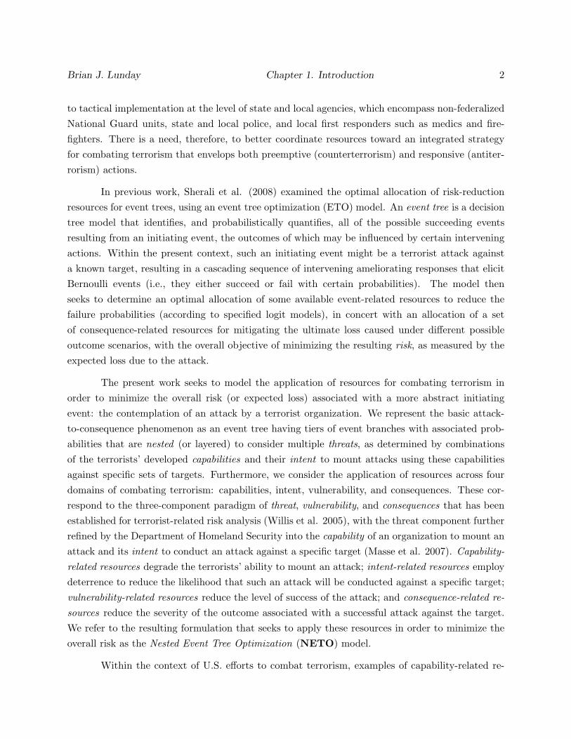
to tactical implementation at the level of state and local agencies, which encompass non-federalizedNational Guard units, state and local police, and local first responders such as medics and fire-fighters. There is a need, therefore, to better coordinate resources toward an integrated strategyfor combating terrorism that envelops both preemptive (counterterrorism) and responsive (antiter-rorism) actions.
In previous work, Sherali et al. (2008) examined the optimal allocation of risk-reductionresources for event trees, using an event tree optimization (ETO) model. An event tree is a decisiontree model that identifies, and probabilistically quantifies, all of the possible succeeding eventsresulting from an initiating event, the outcomes of which may be influenced by certain interveningactions. Within the present context, such an initiating event might be a terrorist attack againsta known target, resulting in a cascading sequence of intervening ameliorating responses that elicitBernoulli events (i.e., they either succeed or fail with certain probabilities). The model thenseeks to determine an optimal allocation of some available event-related resources to reduce thefailure probabilities (according to specified logit models), in concert with an allocation of a setof consequence-related resources for mitigating the ultimate loss caused under different possibleoutcome scenarios, with the overall objective of minimizing the resulting risk, as measured by theexpected loss due to the attack.
The present work seeks to model the application of resources for combating terrorism inorder to minimize the overall risk (or expected loss) associated with a more abstract initiatingevent: the contemplation of an attack by a terrorist organization. We represent the basic attack-to-consequence phenomenon as an event tree having tiers of event branches with associated prob-abilities that are nested (or layered) to consider multiple threats, as determined by combinationsof the terrorists’ developed capabilities and their intent to mount attacks using these capabilitiesagainst specific sets of targets. Furthermore, we consider the application of resources across fourdomains of combating terrorism: capabilities, intent, vulnerability, and consequences. These cor-respond to the three-component paradigm of threat, vulnerability, and consequences that has beenestablished for terrorist-related risk analysis (Willis et al. 2005), with the threat component furtherrefined by the Department of Homeland Security into the capability of an organization to mount anattack and its intent to conduct an attack against a specific target (Masse et al. 2007). Capability-related resources degrade the terrorists’ ability to mount an attack; intent-related resources employdeterrence to reduce the likelihood that such an attack will be conducted against a specific target;vulnerability-related resources reduce the level of success of the attack; and consequence-related re-sources reduce the severity of the outcome associated with a successful attack against the target.We refer to the resulting formulation that seeks to apply these resources in order to minimize theoverall risk as the Nested Event Tree Optimization (NETO) model.
Within the context of U.S. efforts to combat terrorism, examples of capability-related re-

Brian J. Lunday Chapter 1. Introduction 3
sources are military strikes and raids against terrorist training camps, international agency col-laborations to seize financial assets, and military or surrogate-military interdiction of chemical,biological, radiological, nuclear, or high-yield explosive (CBRNE) material during transport andprior to assembly for an attack. Examples of intent-related resources include overt employmentof intelligence assets to detect a planned attack, U.S. Customs inspections at national points ofentry, and visible local security measures such as surveillance, monitoring, and trained personnelto protect the target from attack. Vulnerability-related resources include safety measures for con-taining the damage, such as automated shut-down procedures for a nuclear plant, armored carsto protect political leaders during transport, and electronic devices installed on civilian aircraft todetonate anti-aircraft missiles prior to impact with the fuselage. Some resources have the potentialto affect more than one domain of terrorists’ ability to attack a target. For example, surveillanceresources provide a means of early detection that can be used to reduce capability, intent, or vul-nerability. Therefore, we will consider capability-related, intent-related, and vulnerability-relatedresources under one overall category: countermeasure resources. This contrasts with the remainingcategory of consequence-related resources. Resources belonging to the latter category might includetrained emergency responders, including medics and Weapons of Mass Destruction Civil SupportTeams (WMD-CSTs) to isolate and treat personnel exposed to CBRNE agents, and redundancyin computer networks to mitigate a successful electronic attack on a server.
The principal contributions of the NETO research are threefold. First, we present a novelnested event tree optimization modeling framework that comprehensively addresses capability, in-tent, vulnerability, and consequence issues in combating terrorism. Second, we design alternativereformulations along with effective specialized global optimization algorithms to solve the challeng-ing nonconvex programming problems that result. Third, we provide insights into the effectivenessof different algorithmic and modeling or reformulation strategies via extensive computational testresults, including comparisons with a contemporary commercial software product (BARON).
1.1.2 Network Flow Interdiction with Synergy
During a deployment to Iraq in 2006, the military unit of the author repeatedly encountered twophysical network interdiction problems that share a common structural framework with applica-tions in other areas as well. The first problem was to interdict the flow of material related toExplosively Formed Penetrators (EFPs) and Improvised Explosive Devices (IEDs) into the area ofmilitary operations to prevent assembly and distribution. The second problem was to interdict thedistribution of constructed EFPs and IEDs to various neighborhoods for emplacement. Commonto all these interdiction problems that seek to curtail the accessibility of vertices and arcs withinthe network is the existence of combined multi-tiered resource capabilities. In Iraq, it involved the
Brian J. Lunday Chapter 1. Introduction 4
combination of Iraqi Police, the Iraqi Army, and U.S. Army forces. These agencies had differinginterdiction capabilities, depending on the particular situation. In many cases, the local policeand military were much more effective because they had no language or cultural barriers to impedetheir understanding of the situation and could readily detect ‘out of the ordinary’ circumstances. Inother instances, the U.S. forces were more effective because the indigenous forces were sympatheticto, indifferent to, or possibly even threatened by, the elements trying to evade interdiction. TheU.S. forces had other advantages when serving as interdicting agents, such as having air support,relatively secure communication, and access to various intelligence platforms.
Similar extensions to other interdiction problems occur on various provincial, national, andinternational levels. Within a province or country, law enforcement elements from different echelonsmust cooperate and coordinate efforts. Within the U.S., counter-drug trafficking incorporateselements from the U.S. Coast Guard, U.S. Customs Agency, U.S. Border Patrol, ATF, FBI, StatePolice, and local police. In Saudi Arabia, several divisions from the Ministry of the Interior andMinistry of Defense must coordinate efforts to prevent infiltration of anti-regime elements to theGrand Mosque during the Hajj. Internationally, allied and coalition efforts at network interdictioninvolve law enforcement organizations, militaries, and intelligence agencies of varying capabilitiesand interests, whether they seek to interdict weapons, narcotics, illegal immigrants, or even thespread of information via social networks.
The network interdiction problem has been examined for several decades within the contextof a variety of modeling approaches, optimization objectives, and solution techniques. Pertinent toour effort is the previous research on network interdiction to minimize an adversary’s maximum flowthrough a network, as well as to maximize an adversary’s minimum probability of detection. Ourresearch is further supported by work on the related concept of superadditive synergy, an aspect ofinterpersonal and intergroup dynamics and effectiveness, which has been examined to some extentin the behavioral and social sciences, and has also been only sparingly applied within the field ofoperations research, but not at all within the context of network interdiction.
The principal contributions of the research on network flow interdiction with synergy aretwofold. First, we present novel model formulations for network interdiction that incorporatevarious forms of linear, concave and nonlinear, and general nonlinear synergy relationships betweenresource types. Second, we develop robust solution procedures for each of these cases and conductextensive computational testing to demonstrate that our proposed methods outperform commercialsoftware, particularly on large-sized nonlinear problems.
Brian J. Lunday Chapter 1. Introduction 5
1.1.3 Interdicting Networks to Competitively Minimize Evasion with Synergy
Between Applied Resources
During the aforementioned deployment to Iraq, the military unit of the author encountered twophysical network interdiction problems that motivate this study. The first problem was to interdictthe transport of a kidnapped victim from an assumed origin to a suspected destination. From theopposite perspective, the second problem sought to transport a detainee from a known temporarydetention facility to a long-term internment facility without being detected (and ambushed). Eachof these problems is suitably modeled by a flow occurring from a source to a terminus node overa general network, in which the interdictor attempts to minimize the likelihood of evasion byan agent traversing the network. For the first application, within the context of operations inIraq, interdiction involved the combination of Iraqi Police, the Iraqi Army, and U.S. Army forces.The latter application involved the presence of militias (e.g., 1920 Revolutionary Brigade), terroristorganizations (e.g., Al Qaeda in Iraq), and sympathetically aligned local nationals. In each case, theinterdicting organizations vary in their effectiveness and capabilities and, when deployed together,likely result in a greater (superadditive) level of effectiveness.
Similar network flow interdiction scenarios occur on provincial, national, and internationallevels. For example, within the U.S., counterterrorist efforts to interdict the infiltration of specificpersonnel or weapons-of-mass-destruction incorporate elements from the various echelons of theintelligence and law enforcement communities, and international efforts to enforce non-proliferationtreaties follow the same paradigm, whether they seek to interdict specific personnel, equipment, oreven particular technical knowledge being transmitted over a theoretical network.
The principal contributions of the competitive probability of evasion research are the devel-opment and testing of a framework for alternative resource deployment strategies concerned withminimizing the maximum probability of an adversary evading detection when traversing a network,while incorporating superadditive synergy effects between resources. We also present models thataddress a novel scheme of sequentially deploying subsets of resources overtly and covertly, andconduct comparative analyses with an overt utilization of all resources, with or without synergy.Both theoretical and empirical results are presented to provide insights into threshold criteria foradopting purely overt (with or without synergy) versus composite overt-covert resource utilizationstrategies.
1.1.4 A Dynamic Network Interdiction Problem
The act of interdicting flow through a network is most often modeled in the form of a static two-player, two-stage, sequential game with perfect information (i.e., a Stackelberg game), in which an

Brian J. Lunday Chapter 1. Introduction 6
interdictor allocates resources, followed by the subsequent decisions made by an evader to direct flowthrough the network from a source to a terminus. As with most models, this is a simplification ofreality. Accordingly, in this work we seek to enhance the foregoing modeling approach by consideringthe dynamic interaction between agents within the context of such a network interdiction problem,wherein opponent strategies are not static. A motivation for our model is to provide an applicationframework to examine, and possibly validate, the observe-orient-decide-act cycle (a.k.a., OODAloop), a theory developed by Boyd (1986), which serves as the foundation for military operationalplanning cycles as motivated by his following maxim for successful operations:
“Observe-orient-decide-act more inconspicuously, more quickly, and with more irreg-ularity as basis to keep or gain initiative as well as shape and shift main effort: to re-peatedly and unexpectedly penetrate vulnerabilities and weaknesses exposed by that effortor other effort(s) that tie-up, divert, or drain-away adversary attention (and strength)elsewhere.”
To this end, we extend over the temporal domain the problem of minimizing the maximum flowpertaining to an evader from a single source to a known terminus, considering the simultaneousallocation of multiple resource types to achieve (partial) arc interdictions, but with additionalobjective function penalties as well as an allowance for different durations for the interdictor andevader OODA loops. We then reformulate the model to facilitate a direct solution as a mixed-integer nonlinear program, and we examine stability issues under three conditions for relative looplengths and for two categories of problem structure.
The principal contributions of the dynamic network interdiction research are a novel ex-tension to the existing network interdiction literature that addresses a multi-objective dynamicnetwork interdiction problem, and the examination of related stability, convergence, and computa-tional issues.
1.1.5 Capital Allocation - Equitable Apportionment of Railcars within a Pool-
ing Agreement for Shipping Automobiles
Although the shipment of railcars to transport automobiles from origins to destinations within theU.S. rail network is reliably driven by forecasted consumer demands, the subsequent problem ofrelocating the empty railcars provides great opportunity for improved efficiency. In the absenceof centralized planning, a myopic approach may be to utilize reverse routing, wherein all emptyrailcars are returned to their shipping points-of-origin, resulting in an overestimation of the requiredfleet size and a low utilization rate. Instead, an automobile manufacturer (shipper) and a railroadcompany (carrier) may improve efficiency by meeting the net demands for railcars over the set of
Brian J. Lunday Chapter 1. Introduction 7
shipping origin-destination pairs with the objective of optimizing operating costs, utilization rates,or some multiobjective function. While such approaches may improve efficiency over reverse routingfor one shipper-carrier combination, even greater improvement is possible when the problem isconsolidated over multiple shippers and carriers through a regulated collaborative process, whereinempty railcars are pooled as a common resource with equitable maintenance and replacement costsdistributed among the participants.
Due to inefficiencies created by previous antitrust legislation and an economy that hadevolved to threaten the automobile industry’s competitiveness, the U.S. Government enacted theMotor Carrier Act of 1980 (Public Law 96-296) and the Railroad Transportation Policy Act of1979 (Public Law 96-448), thereby significantly deregulating the trucking and rail industries, re-spectively. The ensuing opportunities, combined with previous recognition of the aforementionedinefficiencies, enabled several companies within the railroad industry to enact a pooling agreementin 1982 and consolidate railcars for shipping automobiles (Sherali and Suharko, 1998). The poolingof railcars requires three recurrent decisions. At the strategic level, a consortium must determinethe optimal fleet size, considering the fluctuations in demands over all origin-destination pairs inthe network. This decision must balance the nature of deliveries, and whether on-time delivery isa hard constraint based on a peak demand forecast or, alternatively, lateness is allowed at a costand within specified tolerances, thereby resulting in a higher overall utilization rate. At the tacticallevel, the ascertained fleet must first be allocated to shippers’ needs and subsequently apportionedamong carriers. The allocation of fleet resources to shippers seeks to balance the objectives of equi-tably allocating railcars and prioritizing the shipper-origin-destination tuples, while incorporatingshippers’ internal priorities in an equitable manner. As a second step at the tactical level, eachshipper’s origin-destination allocations are further allocated to carriers, usually based in proportionto their loaded railcar-days of business with the shipper. Such group decisions need to be enactedby a central agency, and consequently, the shippers established RELOAD R©, a subsidiary of theAssociation of American Railroads (Sherali and Tuncbilek, 1997), to accomplish this task. Since1982, RELOAD R© has become a subsidiary of the TTX Company, and the TTX Reload Group cur-rently coordinates the operations for a fleet of 59,000 automobile railcars provided by nine carriersthat service 17 shippers, with a current savings of over one billion miles per year of empty railcartravel over a reverse routing approach (TTX Company, 2009).
The principal contributions of the capital allocation research in this dissertation are three-fold. First, we improve upon the current industry practice by recognizing its shortcomings withrespect to equity in railcar allocations due to disaggregated problem instances based on graphconnectivity, as well as due to possible alternative optimal flow solutions to the static fleet sizingproblem. Second, we propose four enhanced alternative schemes for allocating railcars to shippersbased respectively on incorporating queuing times in transit to compute proportionality factors for
Brian J. Lunday Chapter 1. Introduction 8
loaded railcar-days (which is demonstrated to yield more equitable solutions); two different tech-niques that utilize a marginal cost analysis; and a game-theoretic approach that employs Shapleyvalue allocations. Third, we provide an insight into a game-theoretic interpretation of the currentrailroad allocation scheme based on Shapley values, and we propose an alternative scheme thatconducts carrier allocations while considering the total capital plus operating costs, rather thansimply capital costs, to derive proportionality factors. For each combination of current and pro-posed shipper and carrier allocation schemes, we test its relative benefit over the current industrystandard with respect to selected metrics using a set of realistic problem instances derived fromdata provided by TTX Company.
1.1.6 Overarching Principles
In order to effectively address resource allocation problems as network programs, we need to adhereto three precepts to avoid the oversimplification of models. First, we must ensure that the scopeof the model is sufficiently broad to account for the interrelated factors that affect the problemat a strategic level. For example, we examine herein the problem of combating terrorism, whereit is insufficient to address only disruption or deterrence of terrorist organizations, interdictionof attacks, or crisis response in isolation. Although funding and deployment priorities for suchoperations are often allocated to different governmental and private agencies, their actions are notindependent. This need for greater coordination of resources, along with a model to account for it,motivates our development of the Nested Event Tree Optimization (NETO) model as well as thecustomized algorithms to robustly solve a breadth of challenging instances.
Second, the models must be sufficiently detailed to account for interactive effects of resourcesat the tactical deployment level. Resources may be co-located, but it would be a folly to expectthis to occur without some impact on their relative effectiveness. Although co-location of resourcesmay induce a positive or negative effect, a negative effect only dissuades their co-location and isless interesting. As such, we consider the effect of superadditive synergistic resource interactionsin the context of the network interdiction problem. We examine such synergy between co-locatedresources on a network for two problem types, wherein an interdictor seeks either to minimize themaximum flow of an evader through a network, or to minimize the maximum probability of evasionby an evader while traversing the network. As an extension, we expand the former model to thetemporal domain to incorporate the dynamic nature of opponent decision cycles, albeit withoutsynergy for our current research, and we examine the stability of strategies under such conditions.
Finally, the solutions to network models must be suitable for implementation. When con-sidering a coalition of decision makers, the suitability of a solution often eludes characterization bya single measure. To elaborate and explore this point, we consider a pooling agreement between
Brian J. Lunday Chapter 1. Introduction 9
automobile shippers and railroads for the fleet sizing and allocation of railcars. Within this con-text, we demonstrate certain inadequacies in the current industry standard and propose alternativeschemes, each characterized by a different metric, and we conduct comparative tests using realisticproblem instances to provide insights and recommendations for industrial implementation.
1.2 Organization of the Dissertation
The remainder of this dissertation is organized as follows. Chapter 2 presents a brief overview ofthe literature pertaining to the nested event tree optimization, network interdiction, and capitalallocation problems.
In Chapter 3, we address the Nested Event Tree Optimization Problem, and we formulate anovel model for applying countermeasure and consequence-management resources to minimize thenet loss due to a terrorist organization and its targeted attacks. For the resulting nonconvex fac-torable program, we design two relaxation-based branch-and-bound algorithms, and also propose apiecewise linear approximation approach that results in a linear, mixed-integer programming modelrepresentation. We further analyze an important fundamental special case of the formulated mod-els, and construct alternative effective relaxations within each of the developed branch-and-boundprocedures for this case. We then design a series of branching and partitioning strategies, as well ascertain range reduction techniques, to enhance algorithmic performance. Extensive computationalresults are presented to test the different outer-approximation mechanisms, in concert with thealternative branching-and-partitioning rule combinations and the range reduction techniques, andto compare this performance to that of the direct mixed-integer formulation approach, as well asto the performance of the commercial package BARON (version 8.1.5). We also conduct a series ofsensitivity analyses to provide insights into algorithmic performance and the effect of various keymodeling parameters on the nature of the solutions produced.
Chapter 4 describes our initial network interdiction research, wherein we present a step-wiseformulation of a model to minimize the maximum flow of an adversary over a network, while ap-plying multiple constrained resources and allowing for partial arc interdiction, and also consideringsuperadditive synergy between resources on each arc. We examine linear, concave and nonlinear,and convex-concave nonlinear synergy relationships to describe the percentage by which an arcis interdicted due to the combined effect of all resource types. For linear synergy relationships,we conduct extensive computational tests to study the sensitivity of various measures of synergyattained at optimality with respect to different problem parameters. For concave nonlinear rela-tionships, which yield convex programs, we develop variants of an inner-linearization procedure andcompare these to the performance of a commercial solver (SBB) designed for convex programs, us-
Brian J. Lunday Chapter 1. Introduction 10
ing a range of specified termination criteria. For convex-concave synergy relationships, we explorevarious approximation granularities and construction techniques for inner-linearizations, piecewiseapproximations, and outer-approximations, and then compare these against the performance ofcommercial solvers designed for convex (SBB) as well as nonconvex (BARON) problems.
In Chapter 5, for the second network interdiction problem, we examine two models thatconsider alternative deployment of resources to maximize the minimum probability of interdictingan adversary traversing a network. The first alternative utilizes all resources overtly, resulting in anonlinear program with constraints that are either linear, concave and nonlinear, or nonconcave andnonlinear, depending on the form of the synergy relationship between resources. We then discussa second alternative, in which resources are echeloned for overt and subsequent covert deployment,thus forgoing synergy in return for the opportunity to deceive the adversary. These formulations aretested to determine the comparative values of the corresponding resource deployment techniques.
We further examine a third network interdiction problem in Chapter 6, in which we proposeand formulate a dynamic network interdiction model that seeks to minimize the maximum value ofa regret function that is comprised of a weighted combination of the interdictor’s costs, the evader’smaximum flow, and the evader’s penalties due to interdiction, and we study stability, convergence,and computational issues related to the players’ strategies.
Chapter 7 addresses the problem of equitably allocating a dynamically-sized fleet of rail-cars to automobile shippers and carriers participating in a pooling agreement. After detailingthe existing fleet sizing and allocation models, we demonstrate the effect of graph connectivityon inequitable decisions made using the current industrial practice, and accordingly, we advocateinstance disaggregation when the underlying network has multiple components. We illustrate an-other inequity-related shortcoming of the present allocation scheme and propose four alternativemechanisms to effectively determine shipper allocations, and another accompanying alternative forcomputing carrier allocations. We then compute and compare shipper and carrier allocations fordifferent combinations of both current and proposed techniques using realistic test problems basedon data obtained from the TTX Company, and we conclude this topic with recommendations forimplementation by the automobile and railroad industries.
Finally, Chapter 8 provides a summary and conclusions of our research contributions, alongwith recommendations for related future research.

Chapter 2
Literature Review
In this chapter, we provide a brief overview of the literature pertaining to the problems investigatedin this dissertation, as well as to the predominant solution methodologies that are adopted in thepresent work.
2.1 Nested Event Tree Optimization
Although we have not encountered previous work that incorporates the breadth of strategic re-source allocations as considered in our Nested Event Tree Optimization approach, several relateddiscussions in the literature have addressed a single tier in this strategic problem. For example,Albores and Shaw (2007) proposed a consequence management model, restricting consideration tothe application of constrained resources to respond to a catastrophic incident (or incidents), andapplied a discrete event simulation approach to study the effect of resource-usage scenarios. Incontrast, Golany et al. (2009) examined an event-focused model within the context of three differ-ent objectives, wherein resource application influences the likelihood of successful terrorist attacksagainst a set of targets via linear relationships, and for which the consequences of a successful attackagainst a given target are fixed. Another notable event-focused model is proposed by Scaparra andChurch (2008), where the authors considered the application of constrained resources to protectcritical infrastructure in the context of a game-theoretic approach, which results in a bilevel integerprogram. Within a game-theoretic context for defending targets from attacks, Zhuang and Bier(2009) developed closed-form solutions for optimal opponent strategies and equilibria for simulta-neous and sequential games for a single target, and extended this investigation to multiple targetgames.
Considering resource applications to influence both event probabilities and consequences
11
Brian J. Lunday Chapter 2. Literature Review 12
of a successful event in a space exploration system, Mehr and Tumer (2006) proposed a multi-objective model to minimize the expected risk as well as its variance, but restrict their model toconsider linear probability-resource relationships. Stranlund and Field (2006) formulated nonlinearmodels to apply constrained event- and consequence-related resources, and studied the effect ofuncertainty on the expected loss. Sherali et al. (2008, 2009) examined the application of event- andconsequence-related resources to reduce the probabilities and outcome costs in order to minimizethe overall risk (expected loss) with a Bernoulli event tree that represents a cascading sequence ofoccurrences following an initiating hazardous event. The authors employed nonlinear logit modelsfor the probability-resource relationships and a linear model for the outcome-resource relationshipsto formulate a nonconvex model, which was solved to global optimality by adopting suitable outer-approximating linear programming relaxations. Developed in 1838 by Verhulst (Pastijn 2006) andadvanced by Berkson (1944), the logit model is useful as a sygmoid function with asymptoticbehavior at both extremes of resource application. Sherali et al. (2008) exploited the logit model’sease of manipulation to solve the formulated nonconvex model to global optimality by adoptinglinear programming relaxations that are constructed via suitable outer-approximations. In anearlier work, Beim and Hobbs (1995) also applied an event tree with conditional probabilities toexamine the net risk, but without the context of strategic planning for resource allocation, so thatthe probabilities in their model are subjectively determined and are fixed.
Dillon and Pate-Cornell (2005) explored the application of suitable resources to minimizethe expected risk in an information system over three distinct tiers — initial failures, intermediatefailures, and total failures — along with the associated cost of failures. While the form of theirobjective function and the use of conditional probabilities most closely align with our approach,they considered a limited set of resource allocation decisions with a discrete probability distribution,resulting in a finitely countable set of feasible solutions that can be explicitly enumerated forobjective value comparison.
Our model formulation in Section 3.2 is a nonlinear, nonconvex program that can be re-cast as a factorable programming problem. Sherali and Wang (2001) have developed a globaloptimization procedure for this general class of problems using Chebyshev interpolating polynomi-als in concert with the Reformulation-Linearization Technique (RLT). Tawarmalani and Sahinidis(2004) have codified a broader taxonomy for applying relaxation-based branch-and-bound proce-dures to solve nonconvex factorable programs, outlining general techniques to convexify nonlinearcomponents that are univariate, bivariate, fractional, multivariate, or composite functions. Ouralgorithmic approach is more closely aligned to the work of Sherali et al. (2008, 2009), in which theauthors reformulate the original problem as per Sherali and Wang (2001), and manipulate the for-mulation so that the inherent nonlinearities are manifested as univariate, monotone (logarithmic)functions. While similar in concept, our solution methodology exploits the particular structure of

Brian J. Lunday Chapter 2. Literature Review 13
our problem, and we also design different tailored procedures to solve a fundamental special caseof our model. In addition, to improve the efficacy of our algorithms, we also incorporate bothfeasibility- and optimality-based range reduction techniques, as recommended in different contextsby Ryoo and Sahinidis (1996), and Sherali and Tuncbilek (1997).
2.2 Network Interdiction Studies
The network interdiction problem has been examined for several decades within the context ofa variety of modeling approaches, optimization objectives, and solution techniques. Pertinentto our efforts in Chapters 4 and 6 is the previous research on network interdiction to minimizean adversary’s maximum flow through a network, and the previous literature on maximizing anadversary’s minimum probability of detection supports our research in Chapter 5. Our researchin both Chapters 4 and 5 is further supported by work on the related concept of superadditivesynergy, an aspect of interpersonal and intergroup dynamics and effectiveness, which has beenexamined to some extent in the behavioral and social sciences, and has also been applied (althoughonly sparingly) within the field of operations research, but not at all within the context of networkinterdiction.
The initial and final phases of our network interdiction research, presented in Chapters 4and 6, respectively, focus on minimizing an adversary’s maximum flow through a network. Wollmer(1964) examined this problem on a planar graph under the assumption of no (or uniform) inter-diction costs, and developed a dynamic programming approach to optimally identify a prescribednumber of arcs for removal (i.e., discrete or binary interdiction). Wollmer (1969), as well as Mc-Masters and Mustin (1970), examined a variant of this work to consider an adversary seeking tominimize a prescribed flow cost through a network, wherein flow costs are linearly proportional tothe arc capacities. Ghare et al. (1971) examined a similar problem, but without the assumptionof a planar graph, and developed an exact branch-and-bound algorithm. This problem was alsoaddressed by Phillips (1993), where it was referred to as the Network Inhibition Problem. Severalvariants were formulated that allow for partial interdiction of arcs, all of which were proven to beNP-Hard. In 1993, Wood published a seminal work for network interdiction modeling, incorporatingexisting graph theory techniques and introducing some new variations to expand the applicabilityof the models. Of particular note, Wood proposed different deterministic network interdiction for-mulations to account for partial arc interdiction, multiple sources and sinks, undirected networks,multiple resources, and multiple commodities, and designed effective solution techniques. Althoughrelated, our models differ sufficiently in concept and structure so as to require the development ofalternative specialized solution methods.
Brian J. Lunday Chapter 2. Literature Review 14
The problem we examine in Chapter 5 concerns maximizing the minimum probability ofdetection, given that an adversary will select a path to traverse from a source node to a terminusnode within a network. Washburn and Wood (1995) studied this problem, which involved applyinga single constrained resource to arcs in a directed network. The authors formulated this instanceas a maximum flow problem by enumerating all the potential paths through the network. Withinthis framework, the authors demonstrated that the optimal interdiction strategy entails placingdetection resources on the arcs belonging to the minimum capacity cut. They also extended theirformulation to consider undirected networks, multiple sources and terminal nodes, multiple evaders,and multiple detection resources, exhibiting for each case the dominance of the strategy that relieson determining the minimum capacity cut(s) for the network. Pan et al. (2003) explored thisproblem assuming a stochastic realization of the adversary’s source and terminal nodes. We alsoadopt a sequential bilevel framework for the detection problem, although we remove the assumptionof omniscience from the adversary’s decisions. In a related problem of detecting an evader locatedwithin a search area (as opposed to traversing a network), Koopman (1979) examines the optimalallocation of constrained search effort, given a probability distribution of the evader’s location andan exponential probability-resource relationship, based on “entirely passive observation” by theinterdictor. Brown (1979) examines a similar spatial search problem, but with the considerationof temporal considerations, both in the probability distribution of the evader’s location and thedetermination of the interdictor’s resource allocations.
Explorations of network interdiction within trilevel optimization frameworks by Brown etal. (2006) and, more recently, Lim and Smith (2008), motivate the final phase of our research inChapter 6. These recent trends account for an increasing number of interactions between opponentsin the interdiction problem and reflect a greater need to shift towards dynamic model formulations.Our dynamic network interdiction model also builds upon the general multi-objective approach ofothers (Royset and Wood, 2007), applying preemptive weights within a nonpreemptive formulation(Sherali and Soyster, 1983).
Other interesting interdiction problems of related interest that are addressed in the literatureinclude stochastic network interdiction (Cormican et al., 1998), multiple commodity interdiction(Lim and Smith, 2007), and shortest path network interdiction (Israeli and Wood, 2002), in whichthe authors have examined variants for the problem of maximizing the shortest path through anetwork by either destroying arcs or increasing their length. The last of these problems is alsostudied by Hemmecke et al. (2003), Held et al. (2005), and Bailey et al. (2006) within a stochasticprogramming context using discrete outcome distributions. Also of note, Brown et al. (2009)examine the interdiction of nuclear weapons in the context of maximizing the length of the criticalpath for their development, rather than in the contexts of our models in Chapters 4–6, where werepresent the interdiction of net flow (e.g., nuclear weapons or their components) during transport
Brian J. Lunday Chapter 2. Literature Review 15
between a given source and terminus.
Our models in Chapters 4 and 5 specifically incorporate synergy between the applied, alignedresources. In a rare quantitative study, von Eye et al. (1998) examined different types of synergyand suggested log-linear models to represent their effects. The authors defined and discussedadditive synergy, conditional additive synergy, and nonadditive synergy, the lattermost of whichincludes superadditive, subadditive, and isolated synergy categories. Additive synergy assumes themere sum of individual effects, which conforms with the types of interactions previously exploredin the literature concerning network interdiction using multiple resources. Moreover, conditionaladditive synergy requires the presence of all agents in order to sum their effects. Within the contextof network interdiction, the resultant interdiction under this type of synergy would be determinedby the scarcest resource, assuming proportional relations between resource availabilities and arcinterdiction costs. Superadditive synergy reflects situations where the total effect is greater thanthe sum of individual parts, and is fundamental to our research. In contrast, subadditive synergyresults in the total effect being less than the sum of individual parts. This concept is not of readilyidentifiable value within the study of network interdiction, nor is isolated synergy, which results inadditional effects due to the presence of multiple agents, but independent of (and separate from) theagents’ individual involvements. Furthermore, the work of Napier and Gershenfeld (1993), whichportends the existence of superadditive synergistic interactions in the presence of no more than fivedifferent resource types, is limited in scope relative to our study in Chapters 4 and 5 because it doesnot examine any specific functional forms to represent synergy, though it does imply a maximumset of resources for which synergy may be attained.
2.3 Equitable Apportionment of Railcars within a Pooling Agree-
ment for Shipping Automobiles
A significant amount of effort has been devoted to the study of transportation problems priorto the pooling agreement, as extensively surveyed in general by Assad (1980) and specifically forempty vehicle fleet management by Dejax and Crainic (1987). Since 1982, additional research hassought to improve the operations within the context of a pooling agreement. In 1985, Glickmanand Sherali employed deterministic models to address three of the unique characteristics of theseproblems. As an enduring principle for future research, they formulated equity-based models tooptimize the sharing of financial benefits from pooling among the individual companies, rather thanstrictly minimizing the aggregated cost of pooled operations. The authors employed decompositionmethods to solve the large-scale models, while providing the ability to exchange different typesof railcars based on requirements and availabilities, and recognizing the additional time and costinvolved to reconfigure between loads. However, exchanges between railcar types such as bilevels

Brian J. Lunday Chapter 2. Literature Review 16
and trilevels are sufficiently infrequent, so that most subsequent research has addressed the problemsof fleet sizing and allocation of each railcar type separately (Sherali and Suharko, 1998). From abroader context involving a cooperative game-theoretic framework for pooled production resources,Sherali and Rajan (1986) used several alternative characteristic functions along with Shapley-valueallocations among participants to examine the propensity for stable coalitions to emerge. Focusingon the fleet-sizing problem, Turnquist and Jordan (1986) formulated models with stochastic traveltimes and examined the trade-offs between fleet size and the probability of short-term shortagesat nodal locations within the network. Beaujon and Turnquist (1991) expanded this work bydeveloping a model to simultaneously determine fleet sizes and vehicle allocations, given stochastictravel times, and designed and tested a heuristic solution procedure.
In the models prior to 1993, the empty railcar demands were assumed to be static, basedon the peak-month forecasts within the horizon considered for fleet sizing in order to preventa stock-out of automobile supplies at dealers (Sherali and Maguire, 2000). As such, the lowerutilization rates during non-peak demand periods required allocation models to provide extensiveanalyses of storage decisions, as in Kikuchi (1985). In contrast, Sherali and Tuncbilek (1997)addressed both the fleet sizing and allocation problems in a deterministic model, but with a dynamicrepresentation of demands and an accounting for stock-out costs, in addition to the costs for idlevehicle storage. Their proposed models reduced overall costs and improved vehicle utilizationrates, based on a decrease in the proposed fleet size by 12-18% over fleet sizes determined by staticmodels. Recognizing the greater level of resolution required to assure shippers and carriers ofsolution viability and equity, Sherali and Suharko (1998) developed detailed multi-objective railcarallocation models that incorporate more specific cost data for late deliveries; discrete stochasticdistributions for travel times; and consideration of equitably scaled dealer priorities by locationfor on-time demand satisfaction. In a more extensive model variant, the authors incorporatedthe industry practice of blocking, which constitutes the consolidation of railcars at an origin formovement to a subset of available destinations.
Despite such progress, the current industry standards exhibit the potential for further im-provement. Our research in Chapter 7 addresses the next step following the strategic planningprocess of determining the total fleet size as per the methodology presented in Sherali and Tunc-bilek (1997) and Sherali and Maguire (2000). This is annotated in the following problem statement:
Given: The total fleet size to be jointly utilized over the next year by the consortium of automobilemanufacturers and railroads participating in the pooling agreement, as determined by theaforementioned strategic planning process (Section 7.2.1 provides further details).
Find: An equitable allocation of railcars to each automobile manufacturer (shipper) from the giventotal fleet size, with a subsequent equitable allocation of railcar acquisition responsibility for

Brian J. Lunday Chapter 2. Literature Review 17
each railroad.
To this end, we consider alternative equity metrics to prescribe railcar allocation mechanismsfor both shippers and carriers, and conduct extensive tests and comparisons using realistic dataacquired from TTX Company in Chicago, Illinois.
Chapter 3
Nested Event Tree Optimization
3.1 Introduction
In this chapter, we present our research on the Nested Event Tree Optimization problem, as in-troduced in Section 1.1.1 and outlined in Section 1.2. In Section 3.2, we formulate the proposedNETO model. In Section 3.3, we design two relaxation-based branch-and-bound algorithms, andalso propose a piecewise linear approximation approach that results in a linear, mixed-integer pro-gramming model representation. We further analyze an important fundamental special case ofthe formulated models, and construct alternative effective relaxations within each of the devel-oped branch-and-bound procedures for this case. In Section 3.4, we propose a series of branchingand partitioning strategies, as well as certain range reduction techniques, to enhance algorith-mic performance. In Section 3.5, we present extensive computational results to test the differentouter-approximation mechanisms in concert with the alternative branching-and-partitioning rulecombinations as well as range reduction techniques, and compare this performance, along with theperformance of the direct mixed-integer formulation approaches, to the performance of the com-mercial package BARON (version 8.1.5). We also conduct a series of sensitivity analyses to provideinsights into algorithmic performance and the effect of various key modeling parameters on thenature of the solutions produced. We conclude this topic in Section 3.6 with a summary, furtherdiscussion, and recommendations for future research.
3.2 Model Formulation
To facilitate our model formulation, we begin by introducing notation for the sets of attack capabil-ities, targets, and outcomes, and for the influencing resource sets that affect related probabilities.
18

Brian J. Lunday Chapter 3. Nested Event Tree Optimization 19
Figure 3.1 depicts the relationship between the defined indices and the associated sets and resourceapplications. Also displayed are the probabilities associated with the tiers of the nested event tree,as defined later in this section, which are affected by the application of countermeasure resourcesand consequence-related resources.
M
ip
A
iinp |
O
innjp |
M
iSs A
nSs O
nSs Rr
injCLoss
…
…
…
n
I nIiNn : nJj
…
i
j
Index sets
Influencing resources
Figure 3.1: Nested event tree displaying indices, resources, and probabilities.
The notation used is defined as follows:
• n ∈ N : set of possible targets.
• i ∈ I: set of possible types of terrorist capabilities for attacks, where:
In = i ∈ I: terrorist capability i could be used against a target n, n ∈ N .
• j ∈ J : set of possible outcomes of the attacks, where:
Jn = j ∈ J : outcome j is a possible occurrence at target n due to some form of attack,n ∈ N .
• S ≡ set of countermeasure resources, where:

Brian J. Lunday Chapter 3. Nested Event Tree Optimization 20
SMi = s ∈ S: resource s can influence the terrorists’ ability to mount an attack using
capability type i, i ∈ I.
SAn = s ∈ S: resource s can influence the terrorists’ intent to attack target n, n ∈ N .
SOn = s ∈ S: resource s can influence the vulnerability of target n with respect to the
possible outcomes at that target, n ∈ N .
Notes:
– STn ≡ SA
n ∪ SOn represents the set of all resources that can be applied to counter
terrorist attacks against a specific target n. This set will be convenient in definingthe decision variables and formulating our proposed model.
– Whenever s ∈ SAn ∩ SO
n , then the effects on the related intent and vulnerabilityprobabilities of the allocation of resource s to target n are suitably determined bycertain logit model coefficients as described later, based on the manner in whichresource s is applied to protect target n.
• R ≡ set of consequence-related resources.
For reference, examples of type types of capabilities, targets, and attack outcomes indexed by i, n,and j are listed in Table 3.1.
Table 3.1: Examples of entities indexed by i, n, and j.Capability Types (i) Target Types (n) Attack Outcomes (j)
Assassination Military base Serious injuriesDirty bombs Political leader FatalitiesKidnapping High population density area Property damages
Chemical attack Water treatment plant Water supply contaminationBiological agents Nuclear power plant Infectious disease propagationNuclear weapons Economic center Economic impact
Remark 3.1. It is possible to further categorize the outcome of a successful attack into the typeof loss and its severity, e.g., dollar value of property damage or number of casualties. However, fornotational convenience, we avoid an additional index to represent different possible levels of severityfor each type of loss by directly defining each attack outcome, j, to be a suitable combination ofsome type and severity of loss. On the other hand, we find merit in differentiating between theterrorists’ ability to develop a capability and the intent to use that capability against a specifictarget. The development of a capability and a defender’s action to deter such a capability couldbe independent of the likelihood of its use against a target. For example, the development of aCBRNE weapon or a nuclear capability might be oriented principally toward inducing terror bythe potential threat of its use without a realized intent to employ it. Assuming that the terrorist

Brian J. Lunday Chapter 3. Nested Event Tree Optimization 21
group acts rationally, it might merely seek to exploit the threatening existence of such a weapon,rather than utilize it based on the developed capability. In effect, the likelihood of its use would beimpacted more by the terrorists’ perceived benefit-cost analysis, namely, that the advancement oftheir cause, as promoted by the actual damage inflicted upon their enemy, outweighs the loss dueto retaliatory response or public outcry and isolation, and future loss of safe bases of operations inneutral-to-supportive regions.
As illustrated in Figure 3.1, the proposed model formulates the problem of combating ter-rorism using the framework of a nested event tree and assuming discrete probability distributions.Our focus is to apply a set of available countermeasure resources (s ∈ S) under a budgetary restric-tion to safeguard a potential set of targets against a known terrorist group, and to mitigate theresulting damage by applying consequence-related resources, thereby minimizing the overall risk,as measured by the total expected loss due to attacks.
Principal Decision Variables:
• (x, y) ≡ overall decision vector, defined as follows:
• x =(xM , xT
), for which
xM ≡(xM
si , s ∈ SMi , i ∈ I
)∈ R
∑i∈I |SM
i |, where each component xMsi represents the amount
of resource type s applied to prevent the terrorists from being able to mount an attackof capability type i.
xT ≡(xT
sn, s ∈ STn , n ∈ N
)∈ R
∑n∈N |ST
n |, where each component xTsn represents the total
amount of resource type s applied at target n to ameliorate the potential intent and/orvulnerability with respect to terrorist attacks.
• y ≡ (yrj , r ∈ R, j ∈ J) ∈ R|R||J |, where yrj represents the amount of consequence-relatedresource r applied to mitigate the loss due to an inflicted attack that produces outcome j.
Intermediate Variables (influenced by (x, y)):
• p =(pM , pA, pO
)a vector of probabilities, defined as follows (see Figure 3.1):
pM ≡(pM
i , i ∈ I), where pM
i represents the probability that the terrorist group can mountan attack using capability type i.
pA ≡(pA(in|i), i ∈ In, n ∈ N
), where pA
(in|i) represents the conditional probability that theterrorist group conducts an attack using capability type i against a potential target n,given that such an attack can be mounted.

Brian J. Lunday Chapter 3. Nested Event Tree Optimization 22
pO ≡(pO(nj|in), i ∈ In, j ∈ Jn, n ∈ N
), where pO
(nj|in) represents the conditional probabilitythat an attack at target n results in outcome j, given that a capability type i attack hasbeen conducted against that target.
• Cinj ≡ loss (cost) incurred when a capability type i attack has been conducted against targetn, resulting in outcome j.
Remark 3.2. As indicated in Remark 3.1, our model differentiates between the probability of theterrorist developing the ability to mount an attack using capability type i (pM
i ), and the probabilitythat an attack is successfully conducted against a particular target n, given this capability (pA
(in|i)).Our motivation here is that these probabilities are not necessarily positively correlated, and more-over, the various aforementioned types of resources can be used to manipulate these probabilities asdelineated below. Note that the product pM
i pA(in|i) represents the probability that an attack using
capability type i is successfully inflicted on target n, and pinj ≡ pMi p
A(in|i)p
O(nj|in) represents the
probability that, further, this successful attack results in outcome j. Furthermore, we utilize theobjective function of minimizing the overall risk, as detailed below. This assumes that all types oflosses can be represented in terms of dollar costs. Otherwise, the model and approach proposedhere would need to be extended to a multi-objective framework.
Remark 3.3. The taxonomy of decision variables is precedented by existing national policies. Forexample, the U.S. National Strategy for Combating Terrorism (NSCT) prescribes three principalactions in order to prevent attacks by terrorist networks. First, it specifies the need to “attackterrorists and their capacity to operate”. This effort is reflected in our model by the applicationof capability-related resources (xM ) that affect the terrorists’ capability to mount attacks across aspectrum of severity levels (with corresponding probabilities pM ). Second, the policy establishesthe priority to “deny terrorists entry to the United States and disrupt their travel internationally”.Within our work, this component is incorporated through the application of intent-related resources(⊆ xT ) that affect the terrorists’ will to attack sets of targets using their developed capabilities(with corresponding probabilities pA). Finally, the NSCT prescribes the defense of potential tar-gets of attack, an effort paralleled by the incorporation of vulnerability-related resources (⊆ xT )that mitigate the effects of successful attacks (with corresponding probabilities pO). The final re-source application in our model is exemplified in the U.S. National Strategy for Homeland Security(NSHS). As a complimentary policy to the NSCT, the NSHS establishes priorities for action withinnational boundaries. In addition to conceptually supporting the domestic application of intent-and vulnerability-related resources (xT ) that reduce the terrorists’ ability to conduct an attack andsuccessfully execute it (with corresponding probabilities pA and pO), the NSHS also directs the useof consequence-management related resources to ”respond to and recover from incidents”. Thispolicy tenet is incorporated within our model via the allocation of consequence-related resources(y) that reduce the costs associated with successful attacks against the given set of targets using

Brian J. Lunday Chapter 3. Nested Event Tree Optimization 23
the developed capabilities (Cinj).
Parameters:
• ξs ≡ amount of countermeasure resource s available, s ∈ S.
• ψr ≡ amount of consequence-related resource r available, r ∈ R.
• a ≡(asi, s ∈ SM
i , i ∈ I), where asi represents the per-unit cost of applying countermeasure
resource s to reduce the ability of the terrorist group to mount a capability type i attack.
• b ≡(bsn, s ∈ ST
n , n ∈ N), where bsn represents the per-unit cost of applying countermeasure
resource s at target n to ameliorate the potential intent and/or vulnerability with respect toterrorist attacks.
• c ≡ (crj , r ∈ R, j ∈ J), where crj represents the per-unit cost of applying consequence-relatedresource r to mitigate the effects of outcome j due to an inflicted attack.
• B ≡ total amount of budget available.
• α ≡(αsi, s ∈ SM
i , i ∈ I): vector of nonnegative constants for defining the logit choice models
for the probabilities pMi (Equation (3.5) below). Moreover, we have:
α0 ≡(α0
i , i ∈ I), where α0
i provides an upper bound on pMi through the logit choice model.
• β ≡(βi
sn, s ∈ SAn , i ∈ In, n ∈ N
): vector of nonnegative constants for defining the logit choice
models for the probabilities pA(in|i) (Equation (3.6) below). Moreover, we have:
β0 ≡(β0i
n , i ∈ In, n ∈ N), where β0i
n provides an upper bound on pA(in|i) through the logit
choice model.
• χ ≡(χin
sj , s ∈ SOn , i ∈ In, j ∈ Jn, n ∈ N
): vector of nonnegative constants for defining the
logit choice models for the probabilities pO(nj|in) (Equation (3.7) below). Moreover, we have:
χ0 ≡(χ0in
j , i ∈ In, j ∈ Jn, n ∈ N), where χ0in
j provides an upper bound on pO(nj|in) through
the logit choice model.
• pMli > 0 and pMu
i < 1 ≡ lower and upper bounds, respectively, for pMi . Considering the case
for the logit choice model (Equation (3.5) below) in which no countermeasure resources are
applied, we have pMui ≤ eα0
i
1+eα0i, ∀ i ∈ I.
• pAl(in|i) > 0 and pAu
(in|i) < 1 ≡ lower and upper bounds, respectively, for pA(in|i). Considering the
case for the logit choice model (Equation (3.6) below) in which no countermeasure resourcesare applied, we have pAu
(in|i) ≤eβ0i
n
1+eβ0in, ∀ (i ∈ In, n ∈ N).
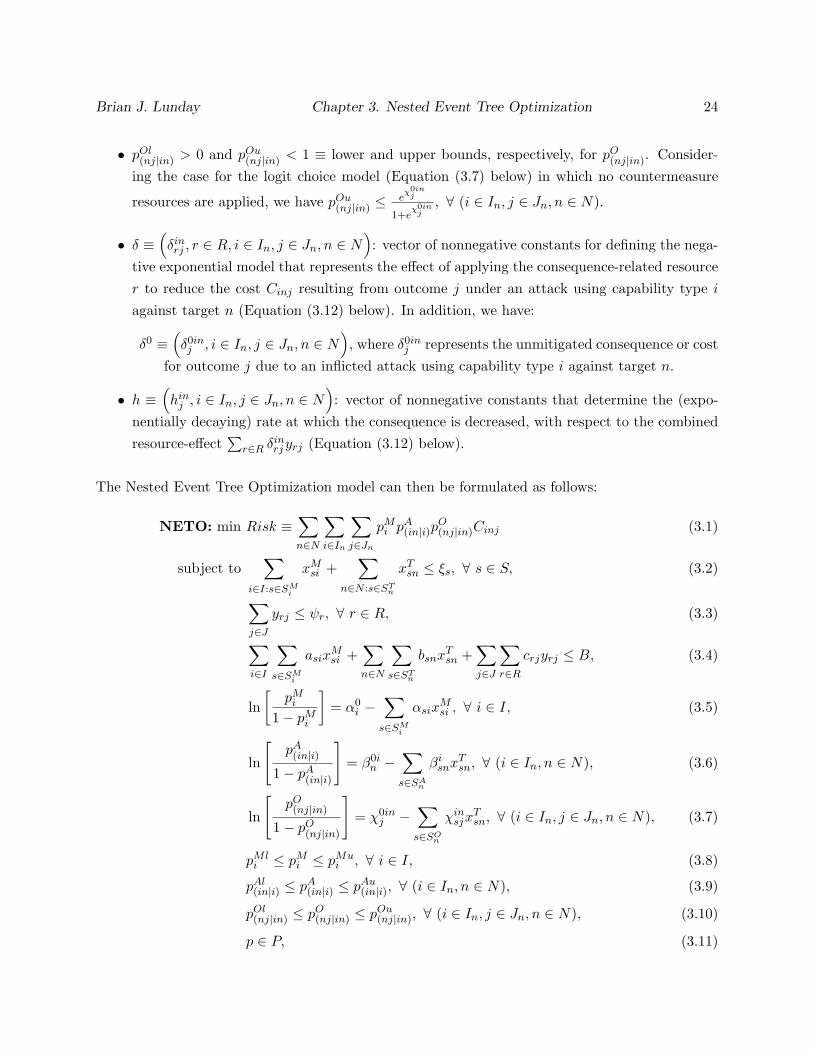
Brian J. Lunday Chapter 3. Nested Event Tree Optimization 24
• pOl(nj|in) > 0 and pOu
(nj|in) < 1 ≡ lower and upper bounds, respectively, for pO(nj|in). Consider-
ing the case for the logit choice model (Equation (3.7) below) in which no countermeasure
resources are applied, we have pOu(nj|in) ≤
eχ0in
j
1+eχ0in
j, ∀ (i ∈ In, j ∈ Jn, n ∈ N).
• δ ≡(δinrj , r ∈ R, i ∈ In, j ∈ Jn, n ∈ N
): vector of nonnegative constants for defining the nega-
tive exponential model that represents the effect of applying the consequence-related resourcer to reduce the cost Cinj resulting from outcome j under an attack using capability type iagainst target n (Equation (3.12) below). In addition, we have:
δ0 ≡(δ0inj , i ∈ In, j ∈ Jn, n ∈ N
), where δ0in
j represents the unmitigated consequence or costfor outcome j due to an inflicted attack using capability type i against target n.
• h ≡(hin
j , i ∈ In, j ∈ Jn, n ∈ N): vector of nonnegative constants that determine the (expo-
nentially decaying) rate at which the consequence is decreased, with respect to the combinedresource-effect
∑r∈R δ
inrjyrj (Equation (3.12) below).
The Nested Event Tree Optimization model can then be formulated as follows:
NETO: min Risk ≡∑n∈N
∑i∈In
∑j∈Jn
pMi p
A(in|i)p
O(nj|in)Cinj (3.1)
subject to∑
i∈I:s∈SMi
xMsi +
∑n∈N :s∈ST
n
xTsn ≤ ξs, ∀ s ∈ S, (3.2)
∑j∈J
yrj ≤ ψr, ∀ r ∈ R, (3.3)
∑i∈I
∑s∈SM
i
asixMsi +
∑n∈N
∑s∈ST
n
bsnxTsn +
∑j∈J
∑r∈R
crjyrj ≤ B, (3.4)
ln[
pMi
1− pMi
]= α0
i −∑
s∈SMi
αsixMsi , ∀ i ∈ I, (3.5)
ln
[pA(in|i)
1− pA(in|i)
]= β0i
n −∑
s∈SAn
βisnx
Tsn, ∀ (i ∈ In, n ∈ N), (3.6)
ln
[pO(nj|in)
1− pO(nj|in)
]= χ0in
j −∑
s∈SOn
χinsjx
Tsn, ∀ (i ∈ In, j ∈ Jn, n ∈ N), (3.7)
pMli ≤ pM
i ≤ pMui , ∀ i ∈ I, (3.8)
pAl(in|i) ≤ p
A(in|i) ≤ p
Au(in|i), ∀ (i ∈ In, n ∈ N), (3.9)
pOl(nj|in) ≤ p
O(nj|in) ≤ p
Ou(nj|in), ∀ (i ∈ In, j ∈ Jn, n ∈ N), (3.10)
p ∈ P, (3.11)
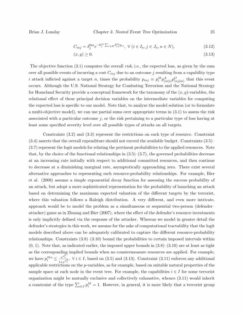
Brian J. Lunday Chapter 3. Nested Event Tree Optimization 25
Cinj = δ0inj e−hin
j
∑r∈R δin
rj yrj , ∀ (i ∈ In, j ∈ Jn, n ∈ N), (3.12)
(x, y) ≥ 0. (3.13)
The objective function (3.1) computes the overall risk, i.e., the expected loss, as given by the sumover all possible events of incurring a cost Cinj due to an outcome j resulting from a capability typei attack inflicted against a target n, times the probability pinj ≡ pM
i pA(in|i)p
O(nj|in) that this event
occurs. Although the U.S. National Strategy for Combating Terrorism and the National Strategyfor Homeland Security provide a conceptual framework for the taxonomy of the (x, y)-variables, therelational effect of these principal decision variables on the intermediate variables for computingthe expected loss is specific to our model. Note that, to analyze the model solution (or to formulatea multi-objective model), we can use partial sums over appropriate terms in (3.1) to assess the riskassociated with a particular outcome j, or the risk pertaining to a particular type of loss having atleast some specified severity level over all possible types of attacks on all targets.
Constraints (3.2) and (3.3) represent the restrictions on each type of resource. Constraint(3.4) asserts that the overall expenditure should not exceed the available budget. Constraints (3.5)–(3.7) represent the logit models for relating the pertinent probabilities to the applied resources. Notethat, by the choice of the functional relationships in (3.5)–(3.7), the governed probabilities decreaseat an increasing rate initially with respect to additional committed resources, and then continueto decrease at a diminishing marginal rate, asymptotically approaching zero. There exist severalalternative approaches to representing such resource-probability relationships. For example, Bieret al. (2008) assume a simple exponential decay function for assessing the success probability ofan attack, but adopt a more sophisticated representation for the probability of launching an attackbased on determining the maximum expected valuation of the different targets by the terrorist,where this valuation follows a Raleigh distribution. A very different, and even more intricate,approach would be to model the problem as a simultaneous or sequential two-person (defender–attacker) game as in Zhuang and Bier (2007), where the effect of the defender’s resource investmentsis only implicitly defined via the response of the attacker. Whereas we model in greater detail thedefender’s strategies in this work, we assume for the sake of computational tractability that the logitmodels described above can be adequately calibrated to capture the different resource-probabilityrelationships. Constraints (3.8)–(3.10) bound the probabilities to certain imposed intervals within(0, 1). Note that, as indicated earlier, the imposed upper bounds in (3.8)–(3.10) are at least as tightas the corresponding implied bounds when no countermeasure resources are applied. For example,we have pMu
i ≤ eα0i
1+eα0i, ∀ i ∈ I, based on (3.5) and (3.13). Constraint (3.11) enforces any additional
applicable restrictions on the p-variables, as for example, based on suitable natural properties of thesample space at each node in the event tree. For example, the capabilities i ∈ I for some terroristorganization might be mutually exclusive and collectively exhaustive, whence (3.11) would inherita constraint of the type
∑i∈I p
Mi = 1. However, in general, it is more likely that a terrorist group

Brian J. Lunday Chapter 3. Nested Event Tree Optimization 26
will develop multiple capabilities at different levels simultaneously. Another special circumstanceoccurs when the outcomes are defined in a manner such that J represents mutually exclusive andcollectively exhaustive levels of intensity or outcome severity, or more generally, when J is indexedover the set of all possible outcome combinations rather than particular outcome events. In suchcases, we can accommodate the appropriate additional sample space-based constraints within (3.11).Constraint (3.12) computes the consequences based on the resources applied to mitigate the effectof the inflicted attacks, and Constraint (3.13) requires nonnegative resource allocations. Note thatsome of the decision variables (x, y) may also be logically restricted to integer values, as for example,when representing trained personnel allocations. However, we shall assume in such cases that anappropriate rounding of such variable values based on an optimal solution derived for ProblemNETO provides an acceptable strategy. Assuming that the specified logit parameters are such thatwe satisfy Constraint (3.11) by substituting x = 0 in Constraints (3.5)–(3.7), the application of noresources yields a feasible solution for Problem NETO, producing an upper bound as given by:
UB0 =∑n∈N
∑i∈In
∑j∈Jn
pMui pAu
(in|i)pOu(nj|in)δ
0inj . (3.14)
We can also derive a lower bound given by:
LB0 =∑n∈N
∑i∈In
∑j∈Jn
pMli pAl
(in|i)pOl(nj|in)C
linj ,
where C linj is a lower bound on each cost, determined by solving:
min Cinj ≡ δ0inj e−hin
j
∑r∈R δin
rj yrj (3.15)
subject to∑r∈R
crjyrj ≤ B,
0 ≤ yrj ≤ ψr, ∀ r ∈ R.
This nonlinear program is equivalent to minimizing the logarithm of Cinj , which yields a linearbounded-variable knapsack problem. The following section discusses a mechanism for comput-ing tighter lower and upper bounds on Problem NETO to design an effective branch-and-boundalgorithm.
3.3 Algorithmic Development
In this section, we propose three reformulations and algorithmic approaches for determining aglobal optimal solution to Problem NETO, including the analysis of a special fundamental case of

Brian J. Lunday Chapter 3. Nested Event Tree Optimization 27
the model in which the generic side-constraint (3.11) is absent, i.e., P ≡ Rn, where n is the numberof p-variables.
3.3.1 Algorithm A1: Convex Relaxations
We begin by reformulating NETO to isolate the inherent nonlinearities into a set of two speciallystructured nonconvex constraint sets having common form, while identifying a hyperrectangle tobound the auxiliary decision variables that are used to define these nonlinear constraint sets. Whilesimilar in concept to Sherali et al. (2008, 2009), in which the authors reformulate the originalproblem as per Sherali and Wang (2001), our solution methodology exploits the particular structureof the NETO Problem, and we also design different tailored procedures to solve a fundamentalspecial case of our model. We then construct a polyhedral outer-approximation to these isolatednonconvex sets and embed this in a branch-and-bound algorithm, which ensures that a sequence ofconvex programs solved over recursively-partitioned hyperrectangles will yield an optimal solutionto NETO (within any prescribed ε-optimality tolerance).
3.3.1.1 Reformulation
Consider the following transformations to simplify the nonlinearities in Problem NETO:
qM1i = ln
(pM
i
), ∀ i ∈ I, (3.16)
qM2i = ln
(1− pM
i
), ∀ i ∈ I, (3.17)
qA1(in|i) = ln
(pA(in|i)
), ∀ (i ∈ In, n ∈ N), (3.18)
qA2(in|i) = ln
(1− pA
(in|i)
), ∀ (i ∈ In, n ∈ N), (3.19)
qO1(nj|in) = ln
(pO(nj|in)
), ∀ (i ∈ In, j ∈ Jn, n ∈ N), (3.20)
qO2(nj|in) = ln
(1− pO
(nj|in)
), ∀ (i ∈ In, j ∈ Jn, n ∈ N). (3.21)
We reference the above original and auxiliary variables in generic terms as pLk and qL
vk, whereL ∈ M,A,O; v ∈ 1, 2; and k ∈ i, (in|i), (nj|in), with these latter indices correspondingrespectively to M,A,O and comprising the sets KL, L ∈ M,A,O. Based on the upper andlower bounds for each intermediate variable, pL
k , we will inherit upper and lower bounds for thecorresponding auxiliary variable, qL
vk, over the appropriately indexed sets, resulting in:
qLlvk ≤ qL
vk ≤ qLuvk < 0, ∀ L, v, (k ∈ KL) ,
Brian J. Lunday Chapter 3. Nested Event Tree Optimization 28
where
qLl1k = ln
(pLl
k
), qLu
1k = ln(pLu
k
), qLl
2k = ln(1− pLu
k
), and qLu
2k = ln(1− pLl
k
), ∀ L, (k ∈ KL) .
(3.22)In order to transform the costs, Cinj , we define
θinj = ln (Cinj) = ln δ0inj − hin
j
∑r∈R
δinrjyrj , ∀ (i ∈ In, j ∈ Jn, n ∈ N). (3.23)
Next, to convexify the objective function, we define
pMi p
A(in|i)p
O(nj|in)Cinj = ezinj , ∀ (i ∈ In, j ∈ Jn, n ∈ N),
which, upon taking the natural logarithm of both sides and using (3.16), (3.18), (3.20), and (3.23),can be equivalently stated as:
zinj = qM1i + qA
1(in|i) + qO1(nj|in) + θinj , ∀ (i ∈ In, j ∈ Jn, n ∈ N). (3.24)
In addition, we bound zinj as follows:zlinj ≤ zinj ≤ zu
inj
where zlinj = ln
(pMl
i pAl(in|i)p
Ol(nj|in)C
linj
)and zu
inj = ln(pMu
i pAu(in|i)p
Ou(nj|in)δ
0inj
) , ∀ (i ∈ In, j ∈ Jn, n ∈ N). (3.25)
Accordingly, we now have a hyperrectangle (Ω) that bounds the intermediate variables as:
Ω =pLl
k ≤ pLk ≤ pLu
k , ∀ L, (k ∈ KL), (3.26)
with an induced hyperrectangle (Φ) that bounds the corresponding auxiliary variables as given by:
Φ =
qLl1k ≤ qL
1k ≤ qLu1k , ∀ L, (k ∈ KL)
qLl2k ≤ qL
2k ≤ qLu2k , ∀ L, (k ∈ KL)
zlinj ≤ zinj ≤ zu
inj , ∀ (i ∈ In, j ∈ Jn, n ∈ N)
. (3.27)
We also define the vectors q ≡(qLvk, ∀ L, v, (k ∈ KL)
)and z ≡ (zinj , ∀ (i ∈ In, j ∈ Jn, n ∈ N)),
and accordingly, we shall refer to (3.27) as (q, z) ∈ Φ. (We similarly refer to (3.26) as p ∈ Ω). Thisresults in the following equivalent reformulation, NETO(Ω), of Problem NETO:
NETO(Ω): min∑n∈N
∑i∈In
∑j∈Jn
ezinj , (3.28)

Brian J. Lunday Chapter 3. Nested Event Tree Optimization 29
subject to∑
i∈I:s∈SMi
xMsi +
∑n∈N :s∈ST
n
xTsn ≤ ξs, ∀ s ∈ S, (3.29)
∑j∈J
yrj ≤ ψr, ∀ r ∈ R, (3.30)
∑i∈I
∑s∈SM
i
asixMsi +
∑n∈N
∑s∈ST
n
bsnxTsn +
∑j∈J
∑r∈R
crjyrj ≤ B, (3.31)
qM1i − qM
2i = α0i −
∑s∈SM
i
αsixMsi , ∀ i ∈ I, (3.32)
qA1(in|i) − q
A2(in|i) = β0i
n −∑
s∈SAn
βisnx
Tsn, ∀ (i ∈ In, n ∈ N), (3.33)
qO1(nj|in) − q
O2(nj|in) = χ0in
j −∑
s∈SOn
χinsjx
Tsn, ∀ (i ∈ In, j ∈ Jn, n ∈ N), (3.34)
zinj = qM1i + qA
1(in|i) + qO1(nj|in) + θinj , ∀ (i ∈ In, j ∈ Jn, n ∈ N), (3.35)
θinj = ln δ0inj − hin
j
∑r∈R
δinrjyrj , ∀ (i ∈ In, j ∈ Jn, n ∈ N). (3.36)
qL1k = ln
(pL
k
), ∀ L, (k ∈ KL) , (3.37)
qL2k = ln
(1− pL
k
), ∀ L, (k ∈ KL) , (3.38)
p ∈ Ω ∩ P, (q, z) ∈ Φ, (x, y) ≥ 0. (3.39)
Note that the formulation NETO(Ω) is linear except for the objective (3.28), which is nonethelessconvex, and the Constraints (3.37)–(3.38), which are, however, nonconvex. We next discuss how tohandle the latter nonconvexity in this reformulated problem.
3.3.1.2 Convex Outer-approximation
To address the nonconvexity within NETO(Ω), we begin by developing a polyhedral outer-approximationfor each of the constraints in Equations (3.37)–(3.38) in order to construct a linearly-constrainedconvex programming relaxation of NETO(Ω), which we will subsequently embed within a branch-and-bound algorithm. The form of Constraints (3.37)–(3.38) can be represented generically asfollows:
τ = ln (σ) , where 0 < σl ≤ σ ≤ σu < 1. (3.40)
The lower bounding affine convex envelope of τ over σ ∈[σl, σu
]is given by:
τ ≥ ln(σl) +ln(σu)− ln(σl)
σu − σl
(σ − σl
), (3.41)

Brian J. Lunday Chapter 3. Nested Event Tree Optimization 30
which is used together with four upper bounding tangential supports to construct the desired outer-approximation, where the points of tangency include the interval endpoints and are equispaced alongthe τ -axis in order to better control the approximation error:
τ ≤ ln(σt) +σ − σt
σt, where σt = e[ln(σl)+
t3(ln(σu)−ln(σl))], t = 0, 1, 2, 3. (3.42)
When Constraints (3.37)–(3.38) are replaced with outer-approximations of the form (3.41)–(3.42),a convex program CP(Ω) results. The following properties readily hold for NETO(Ω) (referredto as Relaxation Properties RP1-RP4 ), given any (possibly further restricted) hyperrectangle Ω,where ν(P) denotes the optimal value for any optimization problem P.
(RP1). By construction, ν [CP(Ω)] is a lower bound on ν [NETO(Ω)].
(RP2). Given (x, y) as part of an optimal solution to CP(Ω), let p and C be computed using theoriginal NETO Constraints (3.5)-(3.7) and (3.12), respectively, as follows:
pMi =
gi
1 + gi, ∀ i ∈ I, where gi = e
α0i−∑
s∈SMi
(αsixMsi ), (3.43)
pA(in|i) =
g(in|i)
1 + g(in|i), ∀ (i ∈ In, n ∈ N), where g(in|i) = e
β0in −
∑s∈SA
n(βi
snxTsn), (3.44)
pO(nj|in) =
g(nj|in)
1 + g(nj|in), ∀ (i ∈ In, j ∈ Jn, n ∈ N), where g(nj|in) = e
χ0inj −
∑s∈SO
n(χin
sj xTsn),
(3.45)
Cinj = δ0inj e−hin
j
∑r∈R(δin
rj yrj), ∀ (i ∈ In, j ∈ Jn, n ∈ N). (3.46)
Then it can be verified that p ∈ Ω (see Sherali et al. (2008) for a similar construction), andso, if p ∈ P , we have that (x, y, p, C) is feasible to NETO, and its objective value in (3.1)yields an upper bound on the optimal values for both Problems NETO and NETO(Ω).
(RP3). If an optimal solution to CP(Ω) satisfies Constraints (3.37)–(3.38), then it is also optimalto NETO(Ω) with the same objective value.
(RP4). Given an optimal solution to CP(Ω), if each of the pLk -variables equals one of its bounds in
the hyperrectangle, Ω, then the solution automatically satisfies Constraints (3.37)–(3.38),and so by RP3, this solution is also optimal to NETO(Ω) with the same objective value.
The cases enumerated in RP3 and RP4 indicate situations when the lower bound (LB) equals theupper bound (UB) computed using RP1 and RP2, respectively. In general, whenever we haveUB− LB ≤ ε, for some tolerance ε ≥ 0, then (x, y, p, C) is ε-optimal to NETO(Ω).

Brian J. Lunday Chapter 3. Nested Event Tree Optimization 31
3.3.1.3 Branch-and-bound Algorithm A1
Consider the following notation:
• a ≡ index for node number in the branch-and-bound tree, where the node has the followingcharacteristics:
Ωa ≡ the hyperrectangle for node a;
wa = (xa, ya, pa, qa, θa, za) ≡ the solution to CP(Ωa);
LBa = ν [CP(Ωa)] ≡ the lower bound on NETO(Ωa) based on wa;
(La,∆a) ≡ the two-tuple (with La ∈ M,A,O and ∆a ∈ KLa) that achieves the maximumabsolute violation in the logarithmic identity (Constraints (3.37)–(3.38)), as determinedby:
(La,∆a) ∈ argmax∣∣∣(qL
1k
)a − ln(pL
k
)a∣∣∣ , ∣∣∣(qL2k
)a − ln(1−
(pL
k
)a)∣∣∣ ,∀ L, (k ∈ KL)
;(3.47)(
pLa∆a
)a≡ the value of the intermediate variable pLa
∆ain the solution wa, indexed by ∆a ∈
KLa , where La ∈ M,A,O, which is used to partition the hyperrectangle at node ainto two hyperrectangles. Specifically,
(pLa∆a
)awill replace the upper bound on pLa
∆ain
one hyperrectangle, and the lower bound in the other;
ζa = (xa, ya, pa, Ca) ≡ the corresponding feasible solution to NETO, given that pa ∈ P ,where:
pa is calculated using xa and Equations (3.43)–(3.45);
Ca is calculated using ya and Equation (3.46);
UBa ≡ an upper bound on NETO computed using Equation (3.1), based on (pa, Ca), giventhat pa ∈ P .
• s ≡ the stage of the branch-and-bound procedure.
• As ≡ the set of active (non-fathomed) nodes in stage s.
• LB(s) ≡ the least lower bound for all active nodes, a ∈ As, i.e., LB(s) ≡ mina∈As
LBa.
• a(s) ≡ the node selected for branching at stage s. This is a node that yields the least lowerbound among the active nodes, i.e., a(s) ∈ argmin
a∈As
LBa.
• ν∗ ≡ the incumbent objective value for NETO with corresponding solution ζ∗.
• ε ≡ the relative % optimality tolerance for terminating the branch-and-bound procedure.

Brian J. Lunday Chapter 3. Nested Event Tree Optimization 32
Step 0. Initialization. Let the incumbent solution ζ∗ correspond to setting x = 0 and y = 0 inProblem NETO, and let ν∗ be the corresponding objective function value as in Equation (3.14).Set s = 0, a = 0, As = 0, and let Ω0 be given by (3.26). Solve CP(Ω0) to find w0 and LB0.Determine ζ0, p0, C0, and UB0. If p0 ∈ P and UB0 < ν∗, then set ν∗ = UB0 and ζ∗ = ζ0. IfLB0 ≥ ν∗(1− ε), then terminate the algorithm and accept the incumbent solution as ε-optimal toNETO. Otherwise, determine (L0,∆0) and proceed to Step 1.
Step 1. Node Selection and Branching Step. Select a node for branching based on theleast lower bound of active nodes, i.e., a(s) ∈ argmin
a∈As
LBa. Branch on the selected node a(s) by
creating two sub-nodes, indexed by a+1 and a+2 and update As+1 = As∪a+ 1, a+ 2−a(s).Define Ωa+1 and Ωa+2 to represent a partitioning of Ωa by replacing pLau
∆a←(pLa∆a
)afor Ωa+1, and
pLal∆a←(pLa∆a
)afor Ωa+2.
Step 2. Bounding Step. For nodes h = a + 1, a + 2 do the following: (a) solve CP(Ωh) todetermine wh and LBh; (b) if LBh < ν∗(1− ε), then determine (Lh,∆h); (c) compute ζh and UBh;and (d) if UBh < ν∗, then let ν∗ = UBh and ζ∗ = ζh. Replace a← a+ 2 and s← s+ 1.
Step 3. Fathoming and Termination Check. For all nodes a ∈ As, if LBa ≥ ν∗(1 − ε), thenupdate As ← As − a. If As = ∅, then terminate the algorithm and accept the incumbent asε-optimal for NETO. Otherwise, return to Step 1.
Proposition 3.1. The proposed branch-and-bound algorithm A1, with ε = 0, either terminatesfinitely with the incumbent solution for Problem CP(Ω) being optimal to Problem NETO, or else aninfinite sequence of stages is generated such that, along any infinite branch of the branch-and-boundtree, any accumulation point of the (x, y, p, C)-variable part of the convex programming relaxationsolutions generated for the corresponding node subproblems solves Problem NETO.
Proof. By the validity of the lower and upper bounds computed by the algorithm, the case of finitetermination is clear. Hence, suppose that an infinite sequence of stages is generated. Consider anyinfinite branch of the branch-and-bound tree generated via the sequence of nested hyperrectanglesΩa(s) that correspond to a set of stages s in some index set S. Thus, we have
LB(s) = LBa(s) = ν[CP(Ωa(s))
], ∀ s ∈ S. (3.48)
For each node a(s), s ∈ S, let wa(s) be the solution to CP(Ω). By taking any convergent subse-quence, if necessary, using the compactness of the feasible region, assume without loss of generality,that
wa(s),Ωa(s)
S→ (w∗,Ω∗). We must show that the solution (x∗, y∗, p∗, C∗), which is a part
of w∗, solves Problem NETO.

Brian J. Lunday Chapter 3. Nested Event Tree Optimization 33
Because LBa(s) is the least lower bound at stage s, we have:
V ∗ ≡ lims→∞,s∈S
LBa(s) ≤ ν [NETO] .
Furthermore, along this infinite branch of the enumeration tree, some pLk -variable, say pL
k, is par-
titioned infinitely over a subset S1 of the nodes S (so that(La(s),∆a(s)
)=(L, k
), ∀ s ∈ S1).
By virtue of the partitioning scheme, it is evident that in the limit, we have either(pL
k
)∗= pLl
k
or(pL
k
)∗= pLu
k. From the construction of the polyhedral outer-approximation (3.41)–(3.42), we
observe that when σ = σl or σ = σu, we have that τ = ln(σ). Hence, in the limit as s→∞, s ∈ S,we get (
qL1k
)∗= ln
[(pL
k
)∗]and
(qL2k
)∗= ln
[1−
(pL
k
)∗]. (3.49)
But for all s ∈ S1, we have from (3.47) that
max∣∣∣(qL
1k
)a(s) − ln(pL
k
)a(s)∣∣∣ , ∣∣∣(qL
2k
)a(s) − ln(1−
(pL
k
)a(s))∣∣∣ ≤
max∣∣∣∣(qL
1k
)a(s)− ln
(pL
k
)a(s)∣∣∣∣ , ∣∣∣∣(qL
2k
)a(s)− ln
(1−
(pL
k
)a(s))∣∣∣∣ , ∀ L, (k ∈ KL) .
(3.50)
Taking limits as s→∞, s ∈ S1, in (3.50), and using (3.49) along withwa(s),Ωa(s)
S→ (w∗,Ω∗),
it follows that w∗ satisfies Equations (3.37)–(3.38). Hence, (x∗, y∗, p∗, C∗) is a feasible solution toProblem NETO with the same objective value V ∗ as for NETO(Ω∗) by RP4. Therefore, we alsohave ν [NETO] ≤ V ∗. Combined with (3.48), we obtain V ∗ = ν [NETO], whereby (x∗, y∗, p∗, C∗)solves Problem NETO.
Corollary 3.1. For ε > 0, the proposed algorithm applied to Problem CP(Ω) will converge to anε-optimal solution for Problem NETO within a finite number of iterations.
Proof. Follows directly from Proposition 3.1.
3.3.1.4 Algorithm A1S: Special Case when P ≡ Rn
We now analyze a fundamental special case of Problem NETO(Ω) given by (3.28)–(3.39) whenP ≡ Rn. In this case, NETO(Ω) is equivalent to relaxing Constraints (3.37)–(3.38), maintainingonly (q, z) ∈ Φ and (x, y) ≥ 0 from (3.39), and adding the relationship:
qL2k = ln (1− eqL
1k), ∀ L, (k ∈ KL) . (3.51)
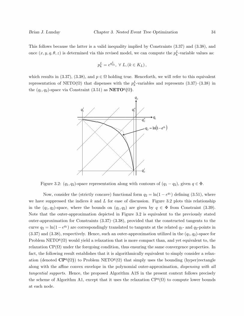
Brian J. Lunday Chapter 3. Nested Event Tree Optimization 34
This follows because the latter is a valid inequality implied by Constraints (3.37) and (3.38), andonce (x, y, q, θ, z) is determined via this revised model, we can compute the pL
k -variable values as:
pLk = eq
L1k , ∀ L, (k ∈ KL) ,
which results in (3.37), (3.38), and p ∈ Ω holding true. Henceforth, we will refer to this equivalentrepresentation of NETO(Ω) that dispenses with the pL
k -variables and represents (3.37)–(3.38) inthe (q1, q2)-space via Constraint (3.51) as NETOq(Ω).
1q
2q
uq2
lq2
uq1
lq1
Vqq 21 of countours
11ln2
qeq
Figure 3.2: (q1, q2)-space representation along with contours of (q1 − q2), given q ∈ Φ.
Now, consider the (strictly concave) functional form q2 = ln(1− eq1) defining (3.51), wherewe have suppressed the indices k and L for ease of discussion. Figure 3.2 plots this relationshipin the (q1, q2)-space, where the bounds on (q1, q2) are given by q ∈ Φ from Constraint (3.39).Note that the outer-approximation depicted in Figure 3.2 is equivalent to the previously statedouter-approximation for Constraints (3.37)–(3.38), provided that the constructed tangents to thecurve q2 = ln(1− eq1) are correspondingly translated to tangents at the related q1- and q2-points in(3.37) and (3.38), respectively. Hence, such an outer-approximation utilized in the (q1, q2)-space forProblem NETOq(Ω) would yield a relaxation that is more compact than, and yet equivalent to, therelaxation CP(Ω) under the foregoing condition, thus ensuring the same convergence properties. Infact, the following result establishes that it is algorithmically equivalent to simply consider a relax-ation (denoted CPq(Ω)) to Problem NETOq(Ω) that simply uses the bounding (hyper)rectanglealong with the affine convex envelope in the polynomial outer-approximation, dispensing with alltangential supports. Hence, the proposed Algorithm A1S in the present context follows preciselythe scheme of Algorithm A1, except that it uses the relaxation CPq(Ω) to compute lower boundsat each node.
Brian J. Lunday Chapter 3. Nested Event Tree Optimization 35
Proposition 3.2. Let CPq(Ω) be as defined above, and let CPq+(Ω) be a relaxation to NETOq(Ω)that augments CPq(Ω) with an arbitrary number of tangential supports to Constraint (3.51), ∀ L, (k ∈ KL).Then ν[CPq(Ω)] = ν[CPq+(Ω)].
Proof. Since CPq(Ω) is a relaxation of CPq+(Ω), it is sufficient to show that an optimal solutionto CPq(Ω) is feasible to CPq+(Ω). Hence, let (x∗, y∗, q∗, θ∗, z∗) solve CPq(Ω). For any generic pair(q1, q2), note that we must have the affine convex envelope in the corresponding outer-approximationactive at this solution, because otherwise, noting Constraints (3.32)–(3.34) and (3.39), we canmaintain feasibility to CPq(Ω) by simultaneously decreasing both q∗1 and q∗2 while keeping q∗1 − q∗2constant (see Figure 3.2), thus reducing the associated z-variable value in (3.35) relative to z∗, andthereby improving the objective function value in (3.28). Hence, (x∗, y∗, q∗, θ∗, z∗) is feasible toCPq+(Ω).
3.3.2 Algorithm A2: Linear Programming (LP) Relaxations
For the second algorithm, we reformulate NETO(Ω) to replace the convex objective function by alower bounding piecewise linear convex supporting function, and combine this with the polyhedralouter-approximation of the nonlinear Constraints (3.37)–(3.38) as previously developed to derivean LP relaxation. Following this, we apply a modification to the recursive partitioning of hyper-rectangles in a branch-and-bound framework to ensure a global optimal solution to NETO (withinany prescribed ε-optimality tolerance).
3.3.2.1 Reformulation of NETO(Ω)
We reformulate NETO(Ω) by rewriting the objective function as:
min∑n∈N
∑i∈In
∑j∈Jn
Zinj , (3.52)
where we incorporate within the constraint set the convex constraints:
Zinj ≥ ezinj , ∀ (i ∈ In, j ∈ Jn, n ∈ N). (3.53)

Brian J. Lunday Chapter 3. Nested Event Tree Optimization 36
3.3.2.2 Outer-approximation to a Linear Program
We now relax NETO(Ω) by replacing (3.53) with four equispaced, lower bounding tangential sup-ports, including those at the two interval end-points:
Zinj ≥ ezt′inj (1 + zinj − zt′
inj), where zt′inj = zl
inj +t′
3
(zuinj − zl
inj
), t′ = 0, 1, 2, 3. (3.54)
When Constraints (3.37)–(3.38) are replaced with outer-approximations of the form (3.41)–(3.42),and furthermore, (3.53) is replaced with a lower-bounding support as in (3.54), a linear programLP(Ω) results. The following Relaxation Properties RP1’-RP4’ hold for LP(Ω):
(RP1’). By construction, ν [LP(Ω)] is a lower bound on ν [NETO(Ω)].
(RP2’). Given (x, y) as part of an optimal solution to LP(Ω), compute p and C using Equations(3.43)–(3.46). If p ∈ P , then (x, y, p, C) is feasible to NETO, and hence yields an upperbound on the optimal values for both Problems NETO and NETO(Ω).
(RP3’). If an optimal solution to LP(Ω) satisfies Constraints (3.37)–(3.38), and zinj = zt′inj for
some t′ ∈ 0, . . . , 3 in (3.54) for each (i ∈ In, j ∈ Jn, n ∈ N), then it is also optimal toNETO(Ω) with the same objective value.
(RP4’). Given an optimal solution to LP(Ω), if each of the pLk -variables equals one of its bounds
in the hyperrectangle, Ω, and if zinj = zt′inj for some t′ ∈ 0, . . . , 3 in (3.54) for each
(i ∈ In, j ∈ Jn, n ∈ N), then this solution is also optimal to NETO(Ω) with the sameobjective value.
Again for LP(Ω), whenever the lower bound (LB) and the upper bound (UB) (computed using RP1’and RP2’, respectively) satisfy UB− LB ≤ ε, then (x, y, p, C) is ε-optimal to Problem NETO(Ω).
3.3.2.3 Branch-and-bound Algorithm A2
We maintain the same notation as before, with the following exceptions:
• wa = (xa, ya, pa, qa, θa, za, Za) ≡ the solution to LP(Ωa).
• LBa = ν [LP(Ωa)] ≡ the lower bound on NETO(Ω) based on wa.
The branch-and-bound algorithmic statement follows that for Algorithm A1, except that the linearprogram LP(Ωa) is solved at each node a in lieu of the nonlinear convex program CP(Ωa) to derivea lower bound. To state the main convergence result for this problem, define Problem NETO’(Ω)
Brian J. Lunday Chapter 3. Nested Event Tree Optimization 37
as the approximation of, or relaxation to, Problem NETO(Ω) in which the objective function(3.28) is replaced with (3.52) along with the supporting Constraint (3.54). Then Problem LP(Ω)is the linearized relaxation of Problem NETO’(Ω) obtained by imposing the polyhedral outer-approximations (3.41)–(3.42) to Constraints (3.37)–(3.38). Furthermore, observe that given anyε′ > 0, by increasing the number of equispaced supports in (3.54) as necessary (to t′(ε′), say), wecan assure that the maximum error between the objective function of NETO(Ω) and its piecewiselinear representation in NETO’(Ω) is no more than ε′. Consequently, the following result holdstrue:
Proposition 3.3. Given any ε > 0, let NETO’(Ω) be defined using t′(ε′) equispaced supports in(3.54), where 0 < ε′ < ε. Then the proposed branch-and-bound algorithm A2, executed with anoptimality tolerance (ε− ε′), will converge to an ε-optimal solution for Problem NETO within afinite number of iterations.
Proof. Similar to the proof of Proposition 3.1 and its corollary, we know that, given (ε− ε′) > 0, theproposed algorithm A2 will converge to an (ε− ε′)-optimal solution for Problem NETO’(Ω) withina finite number of iterations. But the (x, y, p, C)-part of the solution produced for NETO’(Ω) isalso feasible for Problem NETO, with the difference in objective values being bounded above byε′. Hence, by RP1’, the resulting solution is within (ε− ε′) + ε′ = ε of optimality to ProblemNETO.
3.3.2.4 Algorithm A2S: Special Case when P ≡ Rn
Similar to Section 3.3.1.4, when P ≡ Rn, we can apply Algorithm A2 to NETOq(Ω), wherein weutilize the lower bounding relaxation LPq(Ω) as the linearization of CPq(Ω) obtained by replacingthe objective (3.28) with (3.52) along with the supports (3.54). Propositions 2 and 3 (with respectto using the LP relaxation LPq(Ω) in lieu of CPq(Ω)) continue to hold for this special case as well.We henceforth refer to this approach as Algorithm A2S.
3.3.3 Algorithm A3: Mixed-Integer Programming (MIP) Approach
For a third proposed approach, we utilize the linear approximation of the objective function fromNETO’(Ω), but apply a piecewise linear MIP approximation to the nonlinear relationships (3.37)and (3.38) in order to derive a linear mixed-integer program, MIP(Ω), which can then be solveddirectly using standard software. Considering Equations (3.37) and (3.38) stated generically asin Equation (3.40), Proposition 3.4 below motivates the equispacing of approximating segmentbreakpoints along the τ -axis in order to maintain a fixed maximum error over the different segments,which can then be bounded by manipulating the number of segments, T .

Brian J. Lunday Chapter 3. Nested Event Tree Optimization 38
Proposition 3.4. Given a segment of a piecewise linear approximation of the function τ = ln(σ),constructed on σ ∈ [σ1, σ2], where 0 < σl ≤ σ1 < σ2 ≤ σu < 1, define w ≡ ln(σ2) − ln(σ1). Thenthe maximum approximating error, E∗, over [σ1, σ2] depends only on the width w along the ordinalaxis and is given by
E∗ = ln[ew − 1w
]+
w
(ew − 1)− 1. (3.55)
Proof. Define E = τ − τ , where τ is the approximating segment over [σ1, σ2]. Hence, we have:
E = ln(σ)−[(
ln(σ2)− ln(σ1)σ2 − σ1
)(σ − σ1) + ln(σ1)
]. (3.56)
Maximizing the strictly concave function (3.56) using calculus yields
E∗ = ln[
σ2 − σ1
ln(σ2)− ln(σ1)
]− 1 +
σ1 [ln(σ2)− ln(σ1)]
σ2 − σ1
− ln(σ1).
Substituting ln(σ2)− ln(σ1) = w above, along with σ2/σ1 = ew and simplifying, yields (3.55).
Because the segments are equispaced on the τ -axis, Proposition 3.4 asserts that we cancontrol the maximum approximation error simply by adjusting the ordinal segment width, w. Forany specified error tolerance ε > 0, letting wε be the value of w that yields E∗ = ε in (3.55), wecan therefore select the number of segments, T , according to
T =⌈
ln(σu)− ln(σl)wε
⌉. (3.57)
Remark 3.4. For illustration, when [σl, σu] = [0.0001, 0.9999], we get T = 2 in (3.57) forε ∈ [0.0001, 0.10]; and when [σl, σu] = [10−7, 1 − 10−7], Equation (3.57) yields T = 3 for ε ∈[0.0001, 0.07], and T = 2 for ε ∈ [0.08, 0.10].
Considering Equations (3.37) and (3.38) stated generically as in Equation (3.40), a corre-sponding strong linearized MIP approximation of these constraints that yields a partial convex hullrepresentation takes the form (Sherali 2001):
τ =T∑
t=1
[τ t−1λt1 + τ tλt2
]and σ =
T∑t=1
[eτ
t−1λt1 + eτ
tλt2],
where τ t = τ l +t
T
(τu − τ l
), for t = 0, ..., T,
λt1 + λt2 = µt, for t = 1, ..., T, (3.58)

Brian J. Lunday Chapter 3. Nested Event Tree Optimization 39
T∑t=1
µt = 1, (3.59)
(λt1, λt2) ≥ 0 and µt ∈ 0, 1 , ∀ t = 1, ..., T. (3.60)
We found the foregoing MIP approximation representation to suffice in the present contextsince T is typically small (≈ 4); however, Vielma et al. (2009) describe alternative representationsthat might be more suitable for contexts involving a relatively large number of piecewise linearsegments. Hence, we can solve MIP(Ω) directly to obtain a near-optimal solution to ProblemNETO(Ω), wherein the degree of optimality can be controlled via the granularity of the piecewiselinear approximations to (3.37)–(3.38) and the objective function, as governed by T and t′, respec-tively. Note that, given an optimal solution to this MIP, we can derive a corresponding near-optimalsolution to NETO by using Equations (3.43)–(3.46) in a manner similar to applying (RP2)’, where(exact) feasibility is attained provided that the solution satisfies p ∈ P . We henceforth refer to theapplication of this technique as Algorithm A3.
Observe that Algorithm A3 simply provides an approximating near-optimal solution toProblem NETO; determining a precise optimality gap for the resulting solution (provided it isfeasible) via this approach itself is elusive. However, as demonstrated next, for the special casewhen P ≡ Rn, this approach can indeed derive a near-optimal feasible solution along with anoptimality gap assurance.
3.3.3.1 Algorithm A3S: Special Case when P ≡ Rn
For the special case NETOq(Ω) of NETO(Ω) under the condition P ≡ Rn, similar to the approachof Algorithm A3, we construct a linear mixed-integer program MIPq(Ω) by utilizing the tangen-tial approximations (3.52) and (3.54) to the objective function, and by replacing (3.51) with thefollowing MIP approximation, as stated for the generic functional form q2 = ln(1− eq1):
q1 =T∑
t=1
[qt−11 λt1 + qt
1λt2]
and q2 =T∑
t=1
[ln(1− eq
t−11 )λt1 + ln(1− eqt
1)λt2], (3.61)
where qt1 = ql
1 +t
T
(qu1 − ql
1
), for t = 0, ..., T, (3.62)
along with Equations (3.58)–(3.60). (3.63)
Proposition 3.5. ν[MIPq(Ω)] provides a lower bound on ν[NETO].
Proof. Let (x∗, y∗, p∗, C∗) be an optimal solution to NETO, and let us construct a corresponding
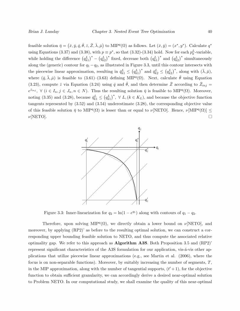
Brian J. Lunday Chapter 3. Nested Event Tree Optimization 40
feasible solution η =(x, y, q, θ, z, Z, λ, µ
)to MIPq(Ω) as follows. Let (x, y) = (x∗, y∗). Calculate q∗
using Equations (3.37) and (3.38), with p ≡ p∗, so that (3.32)-(3.34) hold. Now for each pLk -variable,
while holding the difference(qLk1
)∗ − (qLk2
)∗ fixed, decrease both(qLk1
)∗ and(qLk2
)∗ simultaneouslyalong the (generic) contour for q1−q2, as illustrated in Figure 3.3, until this contour intersects withthe piecewise linear approximation, resulting in qL
k1 ≤(qLk1
)∗ and qLk2 ≤
(qLk2
)∗, along with (λ, µ),where (q, λ, µ) is feasible to (3.61)–(3.63) defining MIPq(Ω). Next, calculate θ using Equation(3.23), compute z via Equation (3.24) using q and θ, and then determine Z according to Zinj =ezinj , ∀ (i ∈ In, j ∈ Jn, n ∈ N). Thus the resulting solution η is feasible to MIPq(Ω). Moreover,noting (3.35) and (3.28), because qL
k1 ≤(qLk1
)∗, ∀ L, (k ∈ KL), and because the objective function
tangents represented by (3.52) and (3.54) underestimate (3.28), the corresponding objective valueof this feasible solution η to MIPq(Ω) is lesser than or equal to ν[NETO]. Hence, ν[MIPq(Ω)] ≤ν[NETO].
1q
2q
uq2
lq2
uq1
lq1
Figure 3.3: Inner-linearization for q2 = ln(1− eq1) along with contours of q1 − q2.
Therefore, upon solving MIPq(Ω), we directly obtain a lower bound on ν[NETO], andmoreover, by applying (RP2)’ as before to the resulting optimal solution, we can construct a cor-responding upper bounding feasible solution to NETO, and thus compute the associated relativeoptimality gap. We refer to this approach as Algorithm A3S. Both Proposition 3.5 and (RP2)’represent significant characteristics of the A3S formulation for our application, vis-a-vis other ap-plications that utilize piecewise linear approximations (e.g., see Martin et al. (2006), where thefocus is on non-separable functions). Moreover, by suitably increasing the number of segments, T ,in the MIP approximation, along with the number of tangential supports, (t′+1), for the objectivefunction to obtain sufficient granularity, we can accordingly derive a desired near-optimal solutionto Problem NETO. In our computational study, we shall examine the quality of this near-optimal
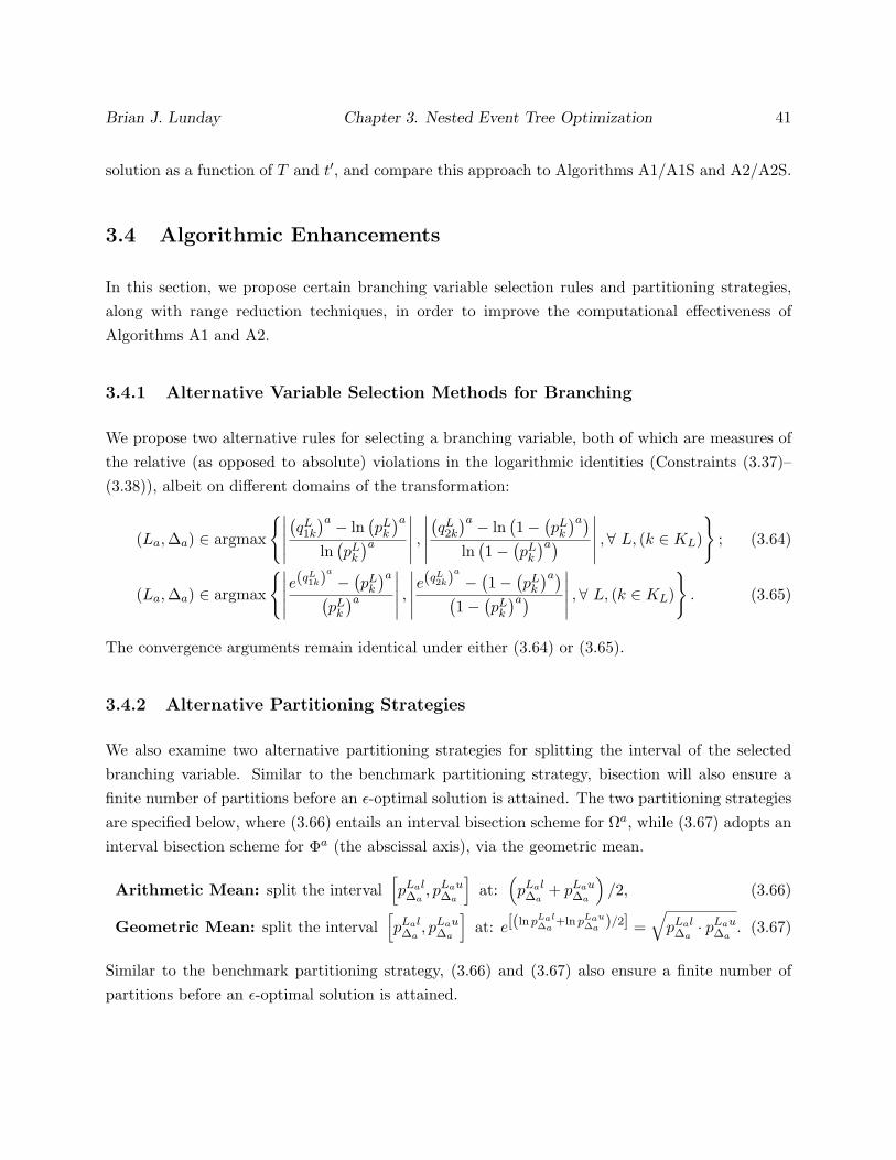
Brian J. Lunday Chapter 3. Nested Event Tree Optimization 41
solution as a function of T and t′, and compare this approach to Algorithms A1/A1S and A2/A2S.
3.4 Algorithmic Enhancements
In this section, we propose certain branching variable selection rules and partitioning strategies,along with range reduction techniques, in order to improve the computational effectiveness ofAlgorithms A1 and A2.
3.4.1 Alternative Variable Selection Methods for Branching
We propose two alternative rules for selecting a branching variable, both of which are measures ofthe relative (as opposed to absolute) violations in the logarithmic identities (Constraints (3.37)–(3.38)), albeit on different domains of the transformation:
(La,∆a) ∈ argmax
∣∣∣∣∣(qL1k
)a − ln(pL
k
)aln(pL
k
)a∣∣∣∣∣ ,∣∣∣∣∣(qL2k
)a − ln(1−
(pL
k
)a)ln(1−
(pL
k
)a)∣∣∣∣∣ ,∀ L, (k ∈ KL)
; (3.64)
(La,∆a) ∈ argmax
∣∣∣∣∣e(qL1k)
a
−(pL
k
)a(pL
k
)a∣∣∣∣∣ ,∣∣∣∣∣e(qL
2k)a
−(1−
(pL
k
)a)(1−
(pL
k
)a)∣∣∣∣∣ ,∀ L, (k ∈ KL)
. (3.65)
The convergence arguments remain identical under either (3.64) or (3.65).
3.4.2 Alternative Partitioning Strategies
We also examine two alternative partitioning strategies for splitting the interval of the selectedbranching variable. Similar to the benchmark partitioning strategy, bisection will also ensure afinite number of partitions before an ε-optimal solution is attained. The two partitioning strategiesare specified below, where (3.66) entails an interval bisection scheme for Ωa, while (3.67) adopts aninterval bisection scheme for Φa (the abscissal axis), via the geometric mean.
Arithmetic Mean: split the interval[pLal∆a, pLau
∆a
]at:
(pLal∆a
+ pLau∆a
)/2, (3.66)
Geometric Mean: split the interval[pLal∆a, pLau
∆a
]at: e[(ln pLal
∆a+ln pLau
∆a)/2] =
√pLal∆a· pLau
∆a. (3.67)
Similar to the benchmark partitioning strategy, (3.66) and (3.67) also ensure a finite number ofpartitions before an ε-optimal solution is attained.

Brian J. Lunday Chapter 3. Nested Event Tree Optimization 42
3.4.3 Range Reduction
We also implement range reduction strategies within our Algorithms A1–A2 as recommended indifferent contexts by Ryoo and Sahinidis (1996), and Sherali and Tuncbilek (1997), which serveto strengthen the underlying relaxations by tightening the bounds defining Ω. (For AlgorithmA3, we apply the range reduction process for Algorithm A2 and then formulate the MIP basedon the resulting tightened intervals.) Specifically, as a pre-processing step at any node a, theimposed interval for each pL
k -variable is updated by solving two linear programs that minimizeand maximize pL
k in turn over the feasible region. Any new bounds for a pLk -variable will induce
corresponding new bounds on the qL1k- and qL
2k-variables by (3.22), as well as on the z-variablesby (3.25). Upon completion of the range reduction process, the polyhedral approximations areupdated as per (3.41)–(3.42). In the case of LP(Ωa), we further impose the objective functionconstraint
∑n∈N
∑i∈In
∑j∈Jn
Zinj ≤ ν∗, where ν∗ is the incumbent objective value, within eachof the range reduction subproblems, and we also update the tangential supports determined by(3.54) based on the revised bounds on the z-variables. This range reduction process is continued ateach new node so long as a sufficient incremental tightening of the bounds results, or until a fixednumber of iterations is reached.
3.5 Computational Testing and Evaluation
We coded Algorithm A1 using C++ and SNOPT 7.2, and Algorithms A2 and A3 using C++ andILOG CPLEX 11.1, and also compared their performance against BARON 8.1.5 using CPLEX forLP subproblems and SNOPT for NLP subproblems. All runs were executed on a computer withan Intel 2.40 GHz Xeon Processor and 1.5 GB of RAM.
3.5.1 Random Generation of Test Instances
We first tested our models over the network structure depicted in Figure 3.1, using 10 randomlygenerated instances having the generic network attributes displayed in Table 3.2, which are listedin increasing order of the number of probability factors considered, and with instance parametersgenerated as follows:
• |I|: integer-valued parameter, generated from a discrete uniform distribution on [2, 4];
• |N |: integer-valued parameter, generated from a discrete uniform distribution on [4, 6], withi ∈ In determined as a Bernoulli outcome with probability 0.75;

Brian J. Lunday Chapter 3. Nested Event Tree Optimization 43
• |J |: integer-valued parameter, generated from a discrete uniform distribution on [4, 6], withj ∈ Jn determined as a Bernoulli outcome with probability 0.75;
• |SM |, |SA|, |SO|, |R|: integer-valued, generated from a uniform distribution on [2, 4];
• |SA ∩ SO|: integer-valued, generated from a uniform distribution on [1, 2];
• ξs = |I|;
• ψr = |J |;
• B = 10 [|I|+∑
n(|In|+ |Jn|)];
• asi, bsn, crj : integer-valued, generated from a uniform distribution on [25, 40];
• αsi, βisn, χ
insj : decimal-valued to the nearest hundredth, generated from a uniform distribution
on [0.50, 1.00];
• α0i , β
0in , χ
0inj : decimal-valued to the nearest hundredth, generated from a uniform distribution
on [−0.05, 0.05];
• pLlk = 0.0001 and pMu
k = min0.9999,no-resource induced upper bound, ∀ L, (k ∈ KL);
• δinrj : decimal-valued to the nearest hundredth, generated from a uniform distribution on
[0.10, 0.50];
• δ0inj : integer-valued, generated from a uniform distribution on [10000, 20000];
• hinj : decimal-valued to the nearest hundredth, generated from a uniform distribution on
[0.90, 1.10].
Table 3.2: Parameter sets for randomly generated instancesInstance |I|
∑n(|In|)
∑n(|Jn|) |SM | |SA| |SA ∩ SO| |SO| |R| Seed*
1 2 6 17 2 4 2 4 3 32 2 8 24 2 4 2 2 2 23 2 9 28 2 2 1 2 3 44 2 9 29 3 3 1 2 4 55 3 10 43 3 3 1 4 2 86 4 12 48 4 2 1 2 4 97 3 12 50 3 3 1 4 4 78 3 12 57 2 4 1 3 3 69 4 13 58 3 4 1 3 3 1010 4 18 75 2 2 2 3 2 1
* The random seed used to generate the instance in C++.
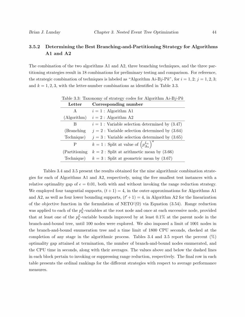
Brian J. Lunday Chapter 3. Nested Event Tree Optimization 44
3.5.2 Determining the Best Branching-and-Partitioning Strategy for Algorithms
A1 and A2
The combination of the two algorithms A1 and A2, three branching techniques, and the three par-titioning strategies result in 18 combinations for preliminary testing and comparison. For reference,the strategic combination of techniques is labeled as “Algorithm Ai-Bj-Pk”, for i = 1, 2; j = 1, 2, 3;and k = 1, 2, 3, with the letter-number combinations as identified in Table 3.3.
Table 3.3: Taxonomy of strategy codes for Algorithm Ai-Bj-PkLetter Corresponding number
A i = 1 : Algorithm A1(Algorithm) i = 2 : Algorithm A2
B i = 1 : Variable selection determined by (3.47)(Branching j = 2 : Variable selection determined by (3.64)Technique) j = 3 : Variable selection determined by (3.65)
P k = 1 : Split at value of(pLa∆a
)a
(Partitioning k = 2 : Split at arithmetic mean by (3.66)Technique) k = 3 : Split at geometric mean by (3.67)
Tables 3.4 and 3.5 present the results obtained for the nine algorithmic combination strate-gies for each of Algorithms A1 and A2, respectively, using the five smallest test instances with arelative optimality gap of ε = 0.01, both with and without invoking the range reduction strategy.We employed four tangential supports, (t+ 1) = 4, in the outer-approximations for Algorithms A1and A2, as well as four lower bounding supports, (t′+1) = 4, in Algorithm A2 for the linearizationof the objective function in the formulation of NETO’(Ω) via Equation (3.54). Range reductionwas applied to each of the pL
k -variables at the root node and once at each successive node, providedthat at least one of the pL
k -variable bounds improved by at least 0.1% at the parent node in thebranch-and-bound tree, until 100 nodes were explored. We also imposed a limit of 1001 nodes inthe branch-and-bound enumeration tree and a time limit of 1800 CPU seconds, checked at thecompletion of any stage in the algorithmic process. Tables 3.4 and 3.5 report the percent (%)optimality gap attained at termination, the number of branch-and-bound nodes enumerated, andthe CPU time in seconds, along with their averages. The values above and below the dashed linesin each block pertain to invoking or suppressing range reduction, respectively. The final row in eachtable presents the ordinal rankings for the different strategies with respect to average performancemeasures.
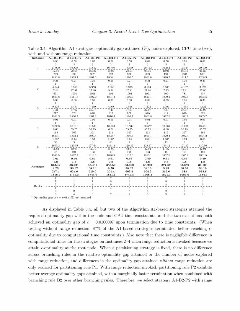
Brian J. Lunday Chapter 3. Nested Event Tree Optimization 45
Table 3.4: Algorithm A1 strategies: optimality gap attained (%), nodes explored, CPU time (sec),with and without range reduction
Instance A1-B1-P1 A1-B1-P2 A1-B1-P3 A1-B2-P1 A1-B2-P2 A1-B2-P3 A1-B3-P1 A1-B3-P2 A1-B3-P3
1
0.56 0.58 0.62 0.56 0.58 0.62 0.56 0.58 0.623 3 3 3 3 3 3 3 3
21.000 16.828 19.812 16.750 16.688 20.172 16.484 17.344 20.10912.91 28.64 26.36 13.07 28.64 26.36 12.91 28.64 26.36229 993 967 227 907 889 197 1001 1001
1813.8 1803.4 1801.3 1808.1 1800.5 1802.0 1810.7 1211.5 1208.9
2
0.21 0.21 0.21 0.21 0.21 0.21 0.21 0.21 0.211 1 1 1 1 1 1 1 1
4.844 3.953 3.953 3.953 3.938 3.984 3.906 4.187 3.9227.43 27.81 27.80 9.26 27.81 27.80 7.43 27.81 27.80631 1001 1001 403 1001 1001 509 781 737
1803.8 1511.7 1507.0 1801.4 1505.5 1623.1 1800.2 1802.0 1803.5
3
0.38 0.38 0.38 0.38 0.38 0.38 0.38 0.38 0.381 1 1 1 1 1 1 1 1
9.125 7.484 7.469 7.468 7.516 7.422 7.797 7.563 7.4227.31 37.97 37.97 7.43 37.97 37.97 7.31 37.97 37.97217 573 573 217 571 575 217 575 575
1808.3 1800.7 1801.2 1816.3 1801.7 1803.8 1812.0 1806.1 1803.2
4
0.91 0.91 0.91 0.91 0.91 0.91 0.91 0.91 0.911 1 1 1 1 1 1 1 1
22.938 18.610 18.531 18.563 18.532 20.657 18.969 19.031 18.5316.66 55.75 55.75 6.76 55.75 55.75 6.66 55.75 55.75115 365 361 111 367 363 115 367 365
1810.1 1803.1 1800.4 1802.7 1807.3 1800.1 1820.4 1802.4 1804.2
5
1.00* 0.74 0.83 1.00* 0.74 0.83 1.00* 0.74 0.8333 3 3 43 3 3 43 3 3
1809.2 120.58 127.64 1871.2 120.32 128.77 1841.2 121.17 130.5611.82 42.94 42.94 11.99 42.94 42.94 11.82 42.94 42.9445 191 193 49 191 193 45 191 191
1856.5 1807.7 1813.2 1826.9 1812.6 1813.1 1862.0 1805.9 1801.5
Averages
0.61 0.56 0.59 0.61 0.56 0.59 0.61 0.56 0.597.8 1.8 1.8 9.8 1.8 1.8 9.8 1.8 1.8
373.42 33.491 35.481 383.59 33.399 36.201 377.67 33.859 36.1099.23 38.62 38.16 9.70 38.62 38.16 9.23 38.62 38.16247.4 624.6 619.0 201.4 607.4 604.2 216.6 583 573.81818.5 1745.3 1744.6 1811.1 1745.5 1768.4 1821.1 1685.6 1684.3
Ranks
7 1 4 7 1 4 7 1 47 1 1 8 1 1 8 1 17 2 4 9 1 6 8 3 51 7 4 3 7 4 1 7 43 9 8 1 7 6 2 5 48 4 3 7 5 6 9 2 1
* Optimality gap of ε = 0.01 (1%) not attained
As displayed in Table 3.4, all but two of the Algorithm A1-based strategies attained therequired optimality gap within the node and CPU time constraints, and the two exceptions bothachieved an optimality gap of ε = 0.0100097 upon termination due to time constraints. (Whentesting without range reduction, 87% of the A1-based strategies terminated before reaching ε-optimality due to computational time constraints.) Also note that there is negligible difference incomputational times for the strategies on Instances 2–4 when range reduction is invoked because weattain ε-optimality at the root node. When a partitioning strategy is fixed, there is no differenceacross branching rules in the relative optimality gap attained or the number of nodes exploredwith range reduction, and differences in the optimality gap attained without range reduction areonly realized for partitioning rule P1. With range reduction invoked, partitioning rule P2 exhibitsbetter average optimality gaps attained, with a marginally faster termination when combined withbranching rule B2 over other branching rules. Therefore, we select strategy A1-B2-P2 with range
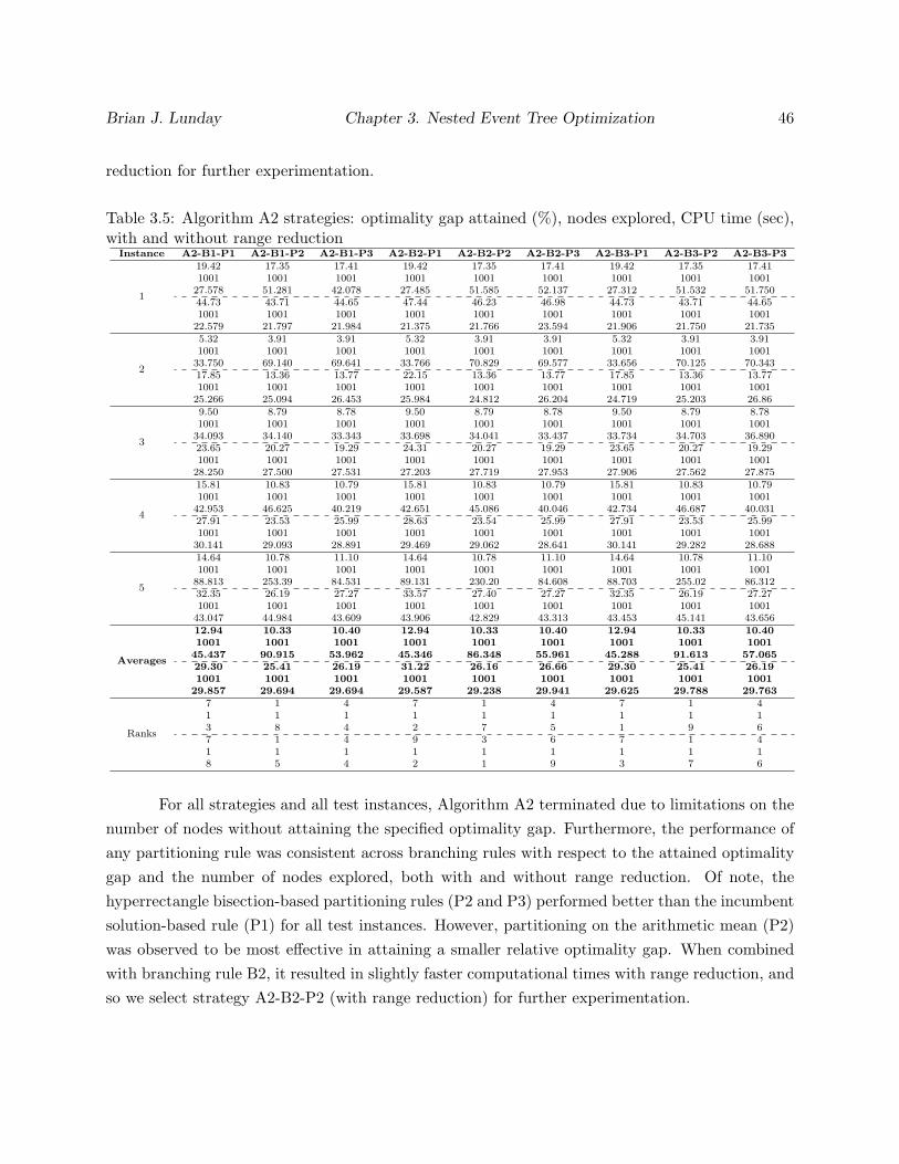
Brian J. Lunday Chapter 3. Nested Event Tree Optimization 46
reduction for further experimentation.
Table 3.5: Algorithm A2 strategies: optimality gap attained (%), nodes explored, CPU time (sec),with and without range reduction
Instance A2-B1-P1 A2-B1-P2 A2-B1-P3 A2-B2-P1 A2-B2-P2 A2-B2-P3 A2-B3-P1 A2-B3-P2 A2-B3-P3
1
19.42 17.35 17.41 19.42 17.35 17.41 19.42 17.35 17.411001 1001 1001 1001 1001 1001 1001 1001 1001
27.578 51.281 42.078 27.485 51.585 52.137 27.312 51.532 51.75044.73 43.71 44.65 47.44 46.23 46.98 44.73 43.71 44.651001 1001 1001 1001 1001 1001 1001 1001 1001
22.579 21.797 21.984 21.375 21.766 23.594 21.906 21.750 21.735
2
5.32 3.91 3.91 5.32 3.91 3.91 5.32 3.91 3.911001 1001 1001 1001 1001 1001 1001 1001 1001
33.750 69.140 69.641 33.766 70.829 69.577 33.656 70.125 70.34317.85 13.36 13.77 22.15 13.36 13.77 17.85 13.36 13.771001 1001 1001 1001 1001 1001 1001 1001 1001
25.266 25.094 26.453 25.984 24.812 26.204 24.719 25.203 26.86
3
9.50 8.79 8.78 9.50 8.79 8.78 9.50 8.79 8.781001 1001 1001 1001 1001 1001 1001 1001 1001
34.093 34.140 33.343 33.698 34.041 33.437 33.734 34.703 36.89023.65 20.27 19.29 24.31 20.27 19.29 23.65 20.27 19.291001 1001 1001 1001 1001 1001 1001 1001 1001
28.250 27.500 27.531 27.203 27.719 27.953 27.906 27.562 27.875
4
15.81 10.83 10.79 15.81 10.83 10.79 15.81 10.83 10.791001 1001 1001 1001 1001 1001 1001 1001 1001
42.953 46.625 40.219 42.651 45.086 40.046 42.734 46.687 40.03127.91 23.53 25.99 28.63 23.54 25.99 27.91 23.53 25.991001 1001 1001 1001 1001 1001 1001 1001 1001
30.141 29.093 28.891 29.469 29.062 28.641 30.141 29.282 28.688
5
14.64 10.78 11.10 14.64 10.78 11.10 14.64 10.78 11.101001 1001 1001 1001 1001 1001 1001 1001 1001
88.813 253.39 84.531 89.131 230.20 84.608 88.703 255.02 86.31232.35 26.19 27.27 33.57 27.40 27.27 32.35 26.19 27.271001 1001 1001 1001 1001 1001 1001 1001 1001
43.047 44.984 43.609 43.906 42.829 43.313 43.453 45.141 43.656
Averages
12.94 10.33 10.40 12.94 10.33 10.40 12.94 10.33 10.401001 1001 1001 1001 1001 1001 1001 1001 1001
45.437 90.915 53.962 45.346 86.348 55.961 45.288 91.613 57.06529.30 25.41 26.19 31.22 26.16 26.66 29.30 25.41 26.191001 1001 1001 1001 1001 1001 1001 1001 1001
29.857 29.694 29.694 29.587 29.238 29.941 29.625 29.788 29.763
Ranks
7 1 4 7 1 4 7 1 41 1 1 1 1 1 1 1 13 8 4 2 7 5 1 9 67 1 4 9 3 6 7 1 41 1 1 1 1 1 1 1 18 5 4 2 1 9 3 7 6
For all strategies and all test instances, Algorithm A2 terminated due to limitations on thenumber of nodes without attaining the specified optimality gap. Furthermore, the performance ofany partitioning rule was consistent across branching rules with respect to the attained optimalitygap and the number of nodes explored, both with and without range reduction. Of note, thehyperrectangle bisection-based partitioning rules (P2 and P3) performed better than the incumbentsolution-based rule (P1) for all test instances. However, partitioning on the arithmetic mean (P2)was observed to be most effective in attaining a smaller relative optimality gap. When combinedwith branching rule B2, it resulted in slightly faster computational times with range reduction, andso we select strategy A2-B2-P2 (with range reduction) for further experimentation.
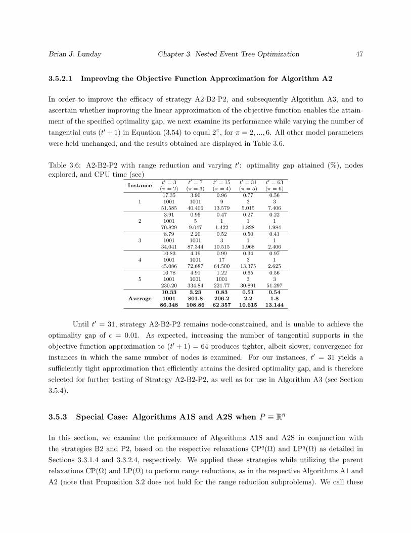
Brian J. Lunday Chapter 3. Nested Event Tree Optimization 47
3.5.2.1 Improving the Objective Function Approximation for Algorithm A2
In order to improve the efficacy of strategy A2-B2-P2, and subsequently Algorithm A3, and toascertain whether improving the linear approximation of the objective function enables the attain-ment of the specified optimality gap, we next examine its performance while varying the number oftangential cuts (t′ + 1) in Equation (3.54) to equal 2π, for π = 2, ..., 6. All other model parameterswere held unchanged, and the results obtained are displayed in Table 3.6.
Table 3.6: A2-B2-P2 with range reduction and varying t′: optimality gap attained (%), nodesexplored, and CPU time (sec)
Instancet′ = 3 t′ = 7 t′ = 15 t′ = 31 t′ = 63
(π = 2) (π = 3) (π = 4) (π = 5) (π = 6)
117.35 3.90 0.96 0.77 0.561001 1001 9 3 3
51.585 40.406 13.579 5.015 7.406
23.91 0.95 0.47 0.27 0.221001 5 1 1 1
70.829 9.047 1.422 1.828 1.984
38.79 2.20 0.52 0.50 0.411001 1001 3 1 1
34.041 87.344 10.515 1.968 2.406
410.83 4.19 0.99 0.34 0.971001 1001 17 3 1
45.086 72.687 64.500 13.375 2.625
510.78 4.91 1.22 0.65 0.561001 1001 1001 3 3
230.20 334.84 221.77 30.891 51.297
Average10.33 3.23 0.83 0.51 0.541001 801.8 206.2 2.2 1.8
86.348 108.86 62.357 10.615 13.144
Until t′ = 31, strategy A2-B2-P2 remains node-constrained, and is unable to achieve theoptimality gap of ε = 0.01. As expected, increasing the number of tangential supports in theobjective function approximation to (t′ + 1) = 64 produces tighter, albeit slower, convergence forinstances in which the same number of nodes is examined. For our instances, t′ = 31 yields asufficiently tight approximation that efficiently attains the desired optimality gap, and is thereforeselected for further testing of Strategy A2-B2-P2, as well as for use in Algorithm A3 (see Section3.5.4).
3.5.3 Special Case: Algorithms A1S and A2S when P ≡ Rn
In this section, we examine the performance of Algorithms A1S and A2S in conjunction withthe strategies B2 and P2, based on the respective relaxations CPq(Ω) and LPq(Ω) as detailed inSections 3.3.1.4 and 3.3.2.4, respectively. We applied these strategies while utilizing the parentrelaxations CP(Ω) and LP(Ω) to perform range reductions, as in the respective Algorithms A1 andA2 (note that Proposition 3.2 does not hold for the range reduction subproblems). We call these
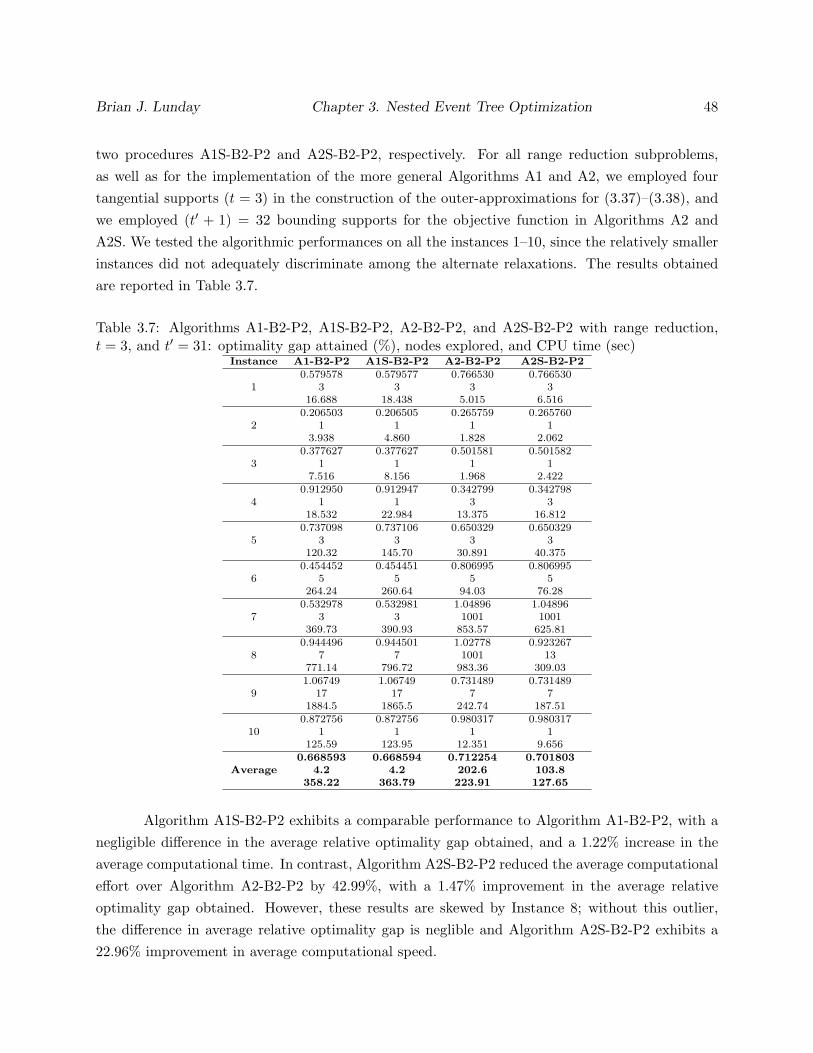
Brian J. Lunday Chapter 3. Nested Event Tree Optimization 48
two procedures A1S-B2-P2 and A2S-B2-P2, respectively. For all range reduction subproblems,as well as for the implementation of the more general Algorithms A1 and A2, we employed fourtangential supports (t = 3) in the construction of the outer-approximations for (3.37)–(3.38), andwe employed (t′ + 1) = 32 bounding supports for the objective function in Algorithms A2 andA2S. We tested the algorithmic performances on all the instances 1–10, since the relatively smallerinstances did not adequately discriminate among the alternate relaxations. The results obtainedare reported in Table 3.7.
Table 3.7: Algorithms A1-B2-P2, A1S-B2-P2, A2-B2-P2, and A2S-B2-P2 with range reduction,t = 3, and t′ = 31: optimality gap attained (%), nodes explored, and CPU time (sec)
Instance A1-B2-P2 A1S-B2-P2 A2-B2-P2 A2S-B2-P2
10.579578 0.579577 0.766530 0.766530
3 3 3 316.688 18.438 5.015 6.516
20.206503 0.206505 0.265759 0.265760
1 1 1 13.938 4.860 1.828 2.062
30.377627 0.377627 0.501581 0.501582
1 1 1 17.516 8.156 1.968 2.422
40.912950 0.912947 0.342799 0.342798
1 1 3 318.532 22.984 13.375 16.812
50.737098 0.737106 0.650329 0.650329
3 3 3 3120.32 145.70 30.891 40.375
60.454452 0.454451 0.806995 0.806995
5 5 5 5264.24 260.64 94.03 76.28
70.532978 0.532981 1.04896 1.04896
3 3 1001 1001369.73 390.93 853.57 625.81
80.944496 0.944501 1.02778 0.923267
7 7 1001 13771.14 796.72 983.36 309.03
91.06749 1.06749 0.731489 0.731489
17 17 7 71884.5 1865.5 242.74 187.51
100.872756 0.872756 0.980317 0.980317
1 1 1 1125.59 123.95 12.351 9.656
Average0.668593 0.668594 0.712254 0.701803
4.2 4.2 202.6 103.8358.22 363.79 223.91 127.65
Algorithm A1S-B2-P2 exhibits a comparable performance to Algorithm A1-B2-P2, with anegligible difference in the average relative optimality gap obtained, and a 1.22% increase in theaverage computational time. In contrast, Algorithm A2S-B2-P2 reduced the average computationaleffort over Algorithm A2-B2-P2 by 42.99%, with a 1.47% improvement in the average relativeoptimality gap obtained. However, these results are skewed by Instance 8; without this outlier,the difference in average relative optimality gap is neglible and Algorithm A2S-B2-P2 exhibits a22.96% improvement in average computational speed.
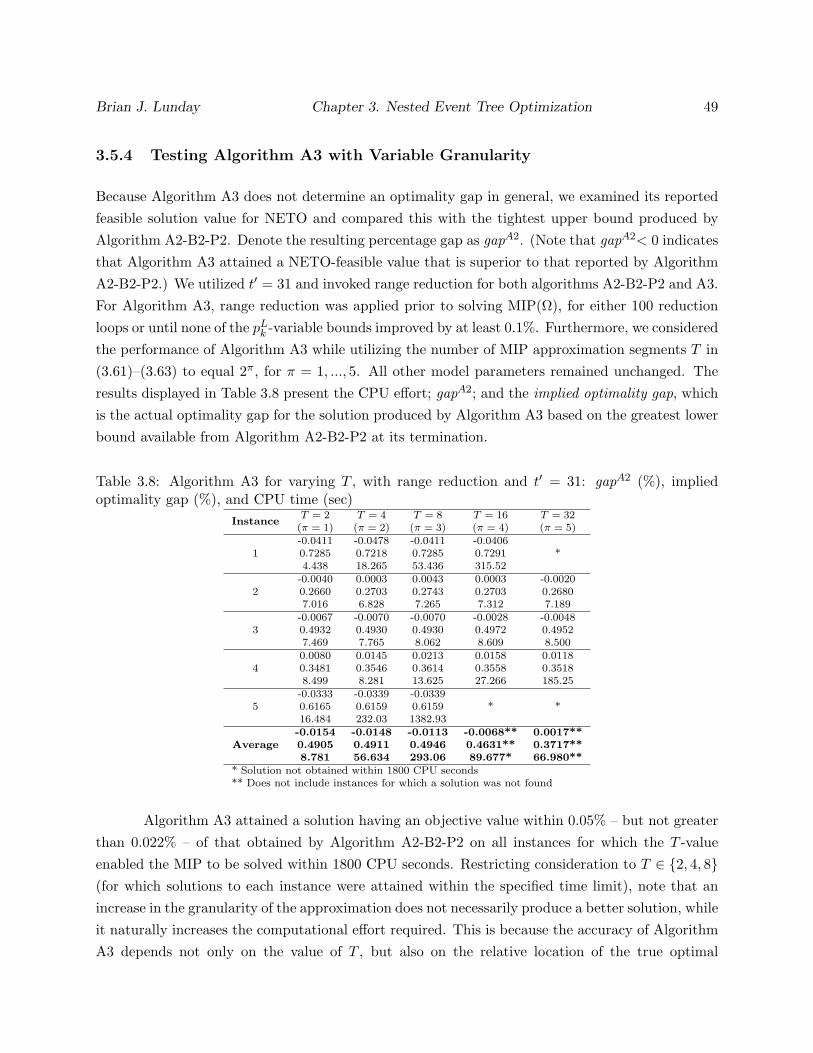
Brian J. Lunday Chapter 3. Nested Event Tree Optimization 49
3.5.4 Testing Algorithm A3 with Variable Granularity
Because Algorithm A3 does not determine an optimality gap in general, we examined its reportedfeasible solution value for NETO and compared this with the tightest upper bound produced byAlgorithm A2-B2-P2. Denote the resulting percentage gap as gapA2. (Note that gapA2< 0 indicatesthat Algorithm A3 attained a NETO-feasible value that is superior to that reported by AlgorithmA2-B2-P2.) We utilized t′ = 31 and invoked range reduction for both algorithms A2-B2-P2 and A3.For Algorithm A3, range reduction was applied prior to solving MIP(Ω), for either 100 reductionloops or until none of the pL
k -variable bounds improved by at least 0.1%. Furthermore, we consideredthe performance of Algorithm A3 while utilizing the number of MIP approximation segments T in(3.61)–(3.63) to equal 2π, for π = 1, ..., 5. All other model parameters remained unchanged. Theresults displayed in Table 3.8 present the CPU effort; gapA2; and the implied optimality gap, whichis the actual optimality gap for the solution produced by Algorithm A3 based on the greatest lowerbound available from Algorithm A2-B2-P2 at its termination.
Table 3.8: Algorithm A3 for varying T , with range reduction and t′ = 31: gapA2 (%), impliedoptimality gap (%), and CPU time (sec)
InstanceT = 2 T = 4 T = 8 T = 16 T = 32(π = 1) (π = 2) (π = 3) (π = 4) (π = 5)
1-0.0411 -0.0478 -0.0411 -0.04060.7285 0.7218 0.7285 0.7291 *4.438 18.265 53.436 315.52
2-0.0040 0.0003 0.0043 0.0003 -0.00200.2660 0.2703 0.2743 0.2703 0.26807.016 6.828 7.265 7.312 7.189
3-0.0067 -0.0070 -0.0070 -0.0028 -0.00480.4932 0.4930 0.4930 0.4972 0.49527.469 7.765 8.062 8.609 8.500
40.0080 0.0145 0.0213 0.0158 0.01180.3481 0.3546 0.3614 0.3558 0.35188.499 8.281 13.625 27.266 185.25
5-0.0333 -0.0339 -0.03390.6165 0.6159 0.6159 * *16.484 232.03 1382.93
Average-0.0154 -0.0148 -0.0113 -0.0068** 0.0017**0.4905 0.4911 0.4946 0.4631** 0.3717**8.781 56.634 293.06 89.677* 66.980**
* Solution not obtained within 1800 CPU seconds** Does not include instances for which a solution was not found
Algorithm A3 attained a solution having an objective value within 0.05% – but not greaterthan 0.022% – of that obtained by Algorithm A2-B2-P2 on all instances for which the T -valueenabled the MIP to be solved within 1800 CPU seconds. Restricting consideration to T ∈ 2, 4, 8(for which solutions to each instance were attained within the specified time limit), note that anincrease in the granularity of the approximation does not necessarily produce a better solution, whileit naturally increases the computational effort required. This is because the accuracy of AlgorithmA3 depends not only on the value of T , but also on the relative location of the true optimal
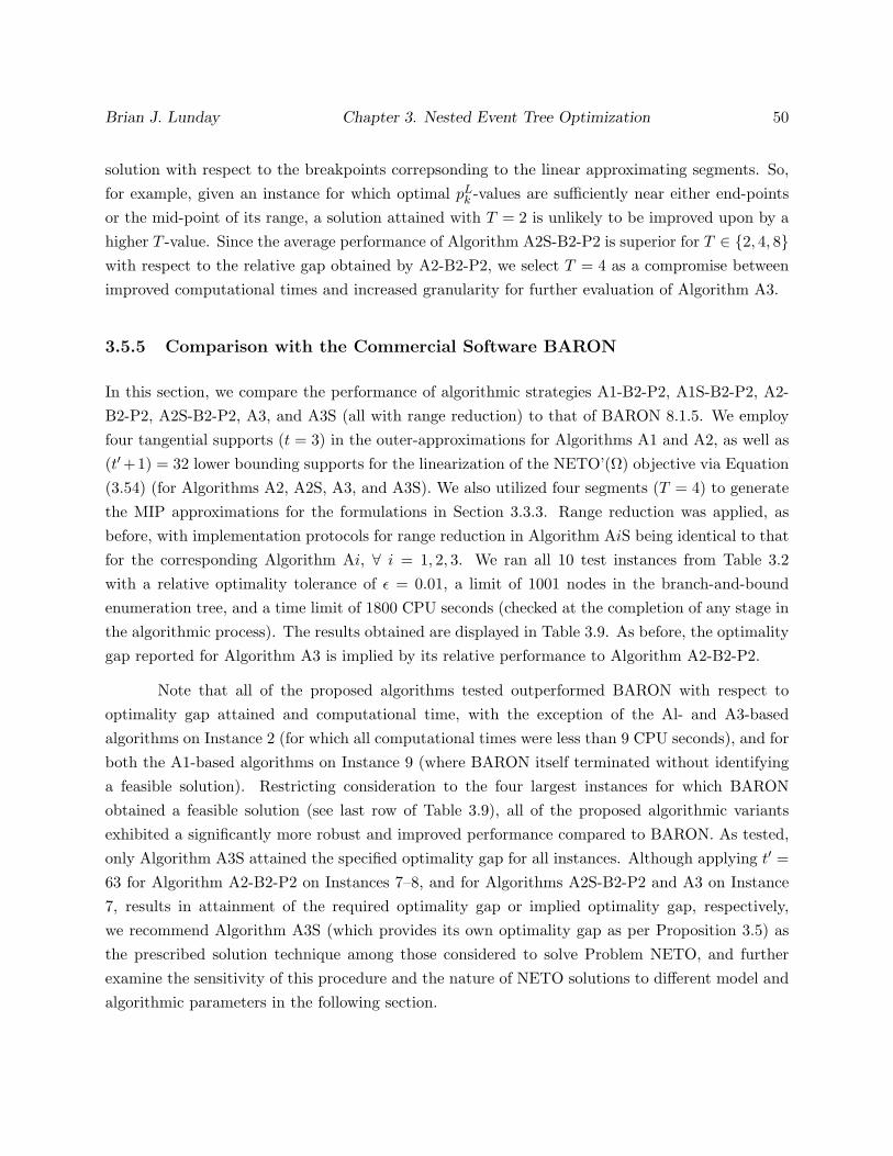
Brian J. Lunday Chapter 3. Nested Event Tree Optimization 50
solution with respect to the breakpoints correpsonding to the linear approximating segments. So,for example, given an instance for which optimal pL
k -values are sufficiently near either end-pointsor the mid-point of its range, a solution attained with T = 2 is unlikely to be improved upon by ahigher T -value. Since the average performance of Algorithm A2S-B2-P2 is superior for T ∈ 2, 4, 8with respect to the relative gap obtained by A2-B2-P2, we select T = 4 as a compromise betweenimproved computational times and increased granularity for further evaluation of Algorithm A3.
3.5.5 Comparison with the Commercial Software BARON
In this section, we compare the performance of algorithmic strategies A1-B2-P2, A1S-B2-P2, A2-B2-P2, A2S-B2-P2, A3, and A3S (all with range reduction) to that of BARON 8.1.5. We employfour tangential supports (t = 3) in the outer-approximations for Algorithms A1 and A2, as well as(t′+1) = 32 lower bounding supports for the linearization of the NETO’(Ω) objective via Equation(3.54) (for Algorithms A2, A2S, A3, and A3S). We also utilized four segments (T = 4) to generatethe MIP approximations for the formulations in Section 3.3.3. Range reduction was applied, asbefore, with implementation protocols for range reduction in Algorithm AiS being identical to thatfor the corresponding Algorithm Ai, ∀ i = 1, 2, 3. We ran all 10 test instances from Table 3.2with a relative optimality tolerance of ε = 0.01, a limit of 1001 nodes in the branch-and-boundenumeration tree, and a time limit of 1800 CPU seconds (checked at the completion of any stage inthe algorithmic process). The results obtained are displayed in Table 3.9. As before, the optimalitygap reported for Algorithm A3 is implied by its relative performance to Algorithm A2-B2-P2.
Note that all of the proposed algorithms tested outperformed BARON with respect tooptimality gap attained and computational time, with the exception of the Al- and A3-basedalgorithms on Instance 2 (for which all computational times were less than 9 CPU seconds), and forboth the A1-based algorithms on Instance 9 (where BARON itself terminated without identifyinga feasible solution). Restricting consideration to the four largest instances for which BARONobtained a feasible solution (see last row of Table 3.9), all of the proposed algorithmic variantsexhibited a significantly more robust and improved performance compared to BARON. As tested,only Algorithm A3S attained the specified optimality gap for all instances. Although applying t′ =63 for Algorithm A2-B2-P2 on Instances 7–8, and for Algorithms A2S-B2-P2 and A3 on Instance7, results in attainment of the required optimality gap or implied optimality gap, respectively,we recommend Algorithm A3S (which provides its own optimality gap as per Proposition 3.5) asthe prescribed solution technique among those considered to solve Problem NETO, and furtherexamine the sensitivity of this procedure and the nature of NETO solutions to different model andalgorithmic parameters in the following section.
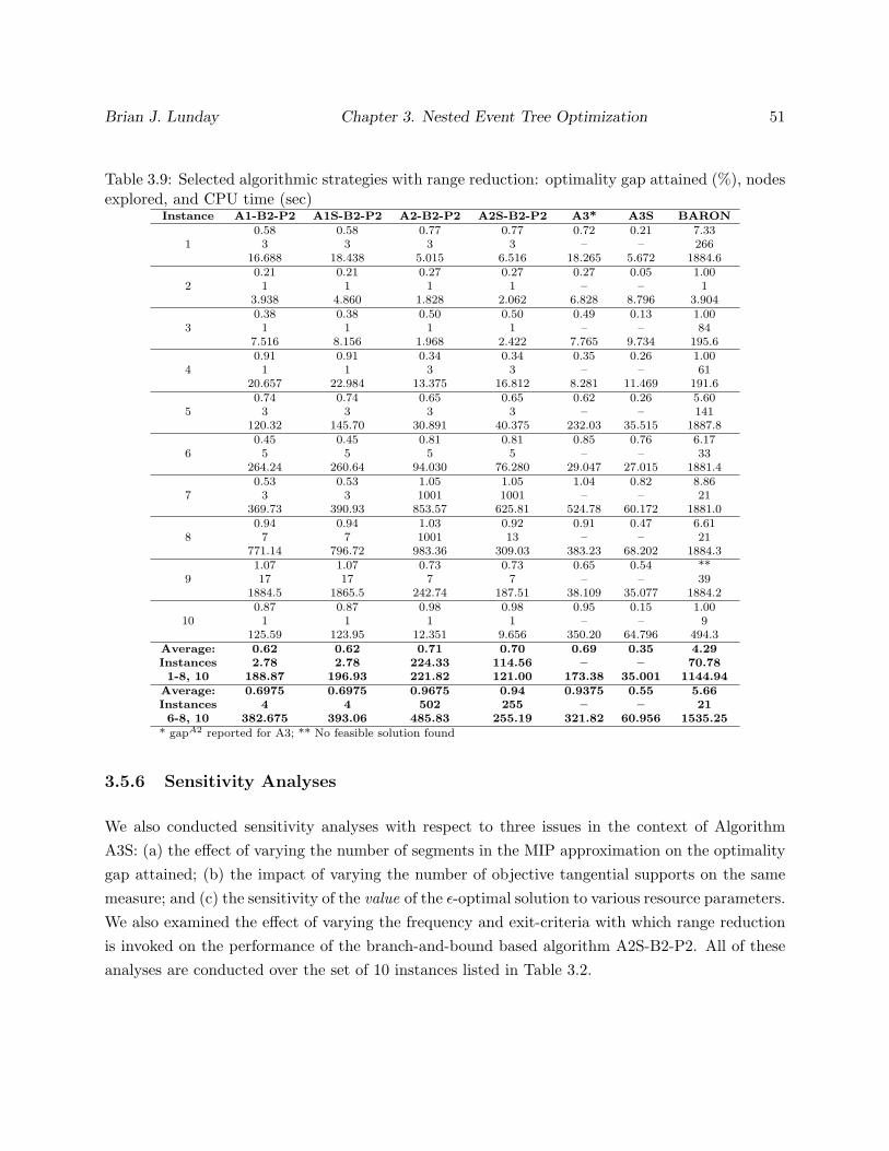
Brian J. Lunday Chapter 3. Nested Event Tree Optimization 51
Table 3.9: Selected algorithmic strategies with range reduction: optimality gap attained (%), nodesexplored, and CPU time (sec)
Instance A1-B2-P2 A1S-B2-P2 A2-B2-P2 A2S-B2-P2 A3* A3S BARON
10.58 0.58 0.77 0.77 0.72 0.21 7.333 3 3 3 – – 266
16.688 18.438 5.015 6.516 18.265 5.672 1884.6
20.21 0.21 0.27 0.27 0.27 0.05 1.001 1 1 1 – – 1
3.938 4.860 1.828 2.062 6.828 8.796 3.904
30.38 0.38 0.50 0.50 0.49 0.13 1.001 1 1 1 – – 84
7.516 8.156 1.968 2.422 7.765 9.734 195.6
40.91 0.91 0.34 0.34 0.35 0.26 1.001 1 3 3 – – 61
20.657 22.984 13.375 16.812 8.281 11.469 191.6
50.74 0.74 0.65 0.65 0.62 0.26 5.603 3 3 3 – – 141
120.32 145.70 30.891 40.375 232.03 35.515 1887.8
60.45 0.45 0.81 0.81 0.85 0.76 6.175 5 5 5 – – 33
264.24 260.64 94.030 76.280 29.047 27.015 1881.4
70.53 0.53 1.05 1.05 1.04 0.82 8.863 3 1001 1001 – – 21
369.73 390.93 853.57 625.81 524.78 60.172 1881.0
80.94 0.94 1.03 0.92 0.91 0.47 6.617 7 1001 13 – – 21
771.14 796.72 983.36 309.03 383.23 68.202 1884.3
91.07 1.07 0.73 0.73 0.65 0.54 **17 17 7 7 – – 39
1884.5 1865.5 242.74 187.51 38.109 35.077 1884.2
100.87 0.87 0.98 0.98 0.95 0.15 1.001 1 1 1 – – 9
125.59 123.95 12.351 9.656 350.20 64.796 494.3Average: 0.62 0.62 0.71 0.70 0.69 0.35 4.29Instances 2.78 2.78 224.33 114.56 – – 70.781-8, 10 188.87 196.93 221.82 121.00 173.38 35.001 1144.94
Average: 0.6975 0.6975 0.9675 0.94 0.9375 0.55 5.66Instances 4 4 502 255 – – 216-8, 10 382.675 393.06 485.83 255.19 321.82 60.956 1535.25
* gapA2 reported for A3; ** No feasible solution found
3.5.6 Sensitivity Analyses
We also conducted sensitivity analyses with respect to three issues in the context of AlgorithmA3S: (a) the effect of varying the number of segments in the MIP approximation on the optimalitygap attained; (b) the impact of varying the number of objective tangential supports on the samemeasure; and (c) the sensitivity of the value of the ε-optimal solution to various resource parameters.We also examined the effect of varying the frequency and exit-criteria with which range reductionis invoked on the performance of the branch-and-bound based algorithm A2S-B2-P2. All of theseanalyses are conducted over the set of 10 instances listed in Table 3.2.
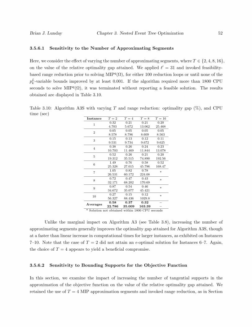
Brian J. Lunday Chapter 3. Nested Event Tree Optimization 52
3.5.6.1 Sensitivity to the Number of Approximating Segments
Here, we consider the effect of varying the number of approximating segments, where T ∈ 2, 4, 8, 16,on the value of the relative optimality gap attained. We applied t′ = 31 and invoked feasibility-based range reduction prior to solving MIPq(Ω), for either 100 reduction loops or until none of thepL
k -variable bounds improved by at least 0.001. If the algorithm required more than 1800 CPUseconds to solve MIPq(Ω), it was terminated without reporting a feasible solution. The resultsobtained are displayed in Table 3.10.
Table 3.10: Algorithm A3S with varying T and range reduction: optimality gap (%), and CPUtime (sec)
Instance T = 2 T = 4 T = 8 T = 16
10.32 0.21 0.21 0.204.703 5.672 13.062 25.468
20.05 0.05 0.05 0.058.578 8.796 8.609 8.563
30.15 0.13 0.12 0.119.531 9.734 9.672 9.625
40.38 0.26 0.24 0.23
10.703 11.469 11.844 13.078
50.52 0.26 0.21 0.20
19.312 35.515 74.890 192.56
61.49 0.76 0.58 0.52
25.328 27.015 45.796 168.47
71.05 0.82 0.78
*26.531 60.172 224.08
80.72 0.47 0.43
*32.171 68.202 170.69
90.87 0.54 0.46
*34.672 35.077 45.421
100.27 0.15 0.12
*56.327 88.436 1029.8
Averages0.58 0.37 0.32 –
22.786 35.009 163.39 –* Solution not obtained within 1800 CPU seconds
Unlike the marginal impact on Algorithm A3 (see Table 3.8), increasing the number ofapproximating segments generally improves the optimality gap attained for Algorithm A3S, thoughat a faster than linear increase in computational times for larger instances, as exhibited on Instances7–10. Note that the case of T = 2 did not attain an ε-optimal solution for Instances 6–7. Again,the choice of T = 4 appears to yield a beneficial compromise.
3.5.6.2 Sensitivity to Bounding Supports for the Objective Function
In this section, we examine the impact of increasing the number of tangential supports in theapproximation of the objective function on the value of the relative optimality gap attained. Weretained the use of T = 4 MIP approximation segments and invoked range reduction, as in Section

Brian J. Lunday Chapter 3. Nested Event Tree Optimization 53
3.5.6.1, in order to facilitate a further comparison of varying t′ instead of T . The results obtainedare displayed in Table 3.11.
Table 3.11: Algorithm A3S with varying t′ and range reduction: optimality gap (%), and CPUtime (sec)
Instance t′ = 31 t′ = 63 t′ = 127 t′ = 255
10.21 0.10 0.063 0.0525.672 7.453 15.265 23.188
20.05 0.015 0.0035 0.00138.796 11.297 15.766 26.765
30.13 0.043 0.021 0.0159.734 12.266 17.531 26.875
40.26 0.082 0.045 0.034
11.469 14.468 19.499 30.015
50.26 0.11 0.073 0.064
35.515 59.093 108.20 184.19
60.76 0.41 0.30 0.28
27.015 35.438 51.609 82.577
70.82 0.23 0.091 0.058
60.172 76.390 139.64 267.67
80.47 0.15 0.095 0.053
68.202 119.33 137.94 329.48
90.54 0.22 0.14 0.12
35.077 51.155 75.718 122.19
100.15 0.069 0.050 0.046
88.436 136.50 237.83 480.37
Averages0.37 0.14 0.088 0.072
35.009 52.339 81.900 157.33
Note first that an increase in t′ improved the value of the optimality gap attained, over allinstances and all stratifications of t′ examined. Over the range of t′-values examined, the greatestimprovement occurred on Instance 7, exhibiting an absolute improvement of 0.762 in the relative(%) optimality gap. The computational times increased less than five-fold on all instances, whilethe number of tangential supports for the objective function increased eight-fold. Compared toincreasing the number of MIP approximating segments, T (see Table 3.10), it is much more effectiveto tighten the linear approximation of the objective function with regard to the attained optimalitygaps and computational times. As ε-optimal solutions were obtained for all t′-values examined, wedeem it sufficient to apply t′ = 31 in order to avoid the significant increases in computational effort.However, should an ε-optimal solution prove elusive within the nodal and time constraints, the firststep in adjusting algorithmic parameters for Algorithm A3S should be to tighten relaxation of theobjective function, rather than tightening the inner-approximation of the constraints.
3.5.6.3 Solution Sensitivity to Resource Availability
Applying Algorithm A3S with T = 4 and t′ = 31, we conducted sensitivity analyses on resourceavailability and its relative effect on the value of the ε-optimal solution, considering an increase by10%, 20%, 30%, and 40% in the parameters ξs, ψr, and B, respectively, for each instance. Our

Brian J. Lunday Chapter 3. Nested Event Tree Optimization 54
instances were not sensitive to increases in the overall budget, as Constraint (3.4) was not active inbaseline studies. However, increasing the countermeasure and consequence-related resources bothdemonstrated improvements in the optimal solution value. Tables 3.12 and 3.13 report the relativechange (%) in the value of the optimal objective function value for each instance, with the bottomrows indicating the average and range of improvements over all instances, for corresponding changesin the ξs and ψr-parameters, respectively.
Table 3.12: Effect of varying ξs on the optimal solution value (%)Instance +10% +20% +30% +40%
1 -2.72 -5.54 -8.48 -11.532 -2.10 -4.14 -6.24 -8.413 -1.53 -3.09 -4.65 -6.254 -2.25 -4.56 -6.95 -9.415 -3.39 -6.96 -10.71 -14.626 -4.72 -9.73 -15.08 -20.697 -2.77 -5.65 -8.66 -11.778 -2.34 -4.80 -7.34 -9.999 -3.25 -6.64 -10.13 -13.7310 -1.67 -3.36 -5.08 -6.84
Average -2.67 -5.45 -8.33 -11.32Range [-4.72,-1.53] [-9.73,-3.09] [-15.08,-4.65] [-20.69,-6.25]
Table 3.13: Effect of varying ψr on the optimal solution value (%)Instance +10% +20% +30% +40%
1 -2.80 -5.63 -8.58 -11.602 -1.24 -2.48 -3.73 -4.983 -1.81 -3.63 -5.46 -7.324 -2.34 -4.73 -7.17 -9.635 -1.14 -2.29 -3.44 -4.586 -2.07 -4.19 -6.35 -8.597 -2.16 -4.35 -6.58 -8.848 -1.41 -2.83 -4.26 -5.709 -1.43 -2.88 -4.35 -5.7910 -0.61 -1.21 -1.81 -2.40
Average -1.70 -3.42 -5.17 -6.94Range [-2.80,-0.61] [-5.63,-1.21] [-8.58,-1.81] [-11.60,-2.40]
In response to an increase in the countermeasure resources ξs, ∀s ∈ S, the objective func-tion value decreased in near-linear proportions. Average performances are displayed in Table 3.12,where for our test instances, the objective function values were reduced by approximately 66.33%on average from the corresponding values when no resources are applied. As it turns out, ad-ditional resources are applied where they are most effective, viz, near the points of inflection onthe logit probability-resource relationships, ensuring the greatest marginal effect on probabilitieswith a near-linear relationship. Linearly proportional increases in the consequence-related resourcesψr, ∀ r ∈ R, also cause a similar near-linear improvement, based on the application of additionalresources to Constraint (3.12). Further, the improvement in the objective function value for aproportional increase in the consequence-related resources ψr was only 61–64% as effective as anidentical proportional increase in the countermeasure resources ξs, on average, though this result
Brian J. Lunday Chapter 3. Nested Event Tree Optimization 55
does not hold uniformly. For Instances 1, 3, and 4, proportional increases in ψr were actually moreeffective at reducing the optimal objective function value, indicating that a broader generalizationis elusive.
3.5.6.4 Algorithmic Sensitivity to Range Reduction Parameters
In this section, we examine the sensitivity of the performance measures for Algorithm A2S-B2-P2by varying certain range reduction technique parameters, in order to determine whether it canoutperform Algorithm A3S. We selected Algorithm A2S-B2-P2 with (t′ + 1) = 32 and T = 4over other branch-and-bound algorithms because it obtained ε-optimal solutions for nine of the teninstances in Table 3.9, which is more than for any other candidate algorithm. Optimality-basedrange reduction was applied to each of the pL
k -variables at the root node and once at each successivenode, provided that at least one of the pL
k -variable bounds improved by at least 0.1% at the parentnode in the branch-and-bound tree, until 100 nodes were explored. However, we considered applyingrange reduction a total of RRnode ∈ 1, 2, 3 times at each node until an exit-criterion was triggered.We imposed a limit of 1001 nodes in the branch-and-bound enumeration tree and a time limit of1800 CPU seconds, checked at the completion of any stage in the algorithmic process. Displayed inTable 3.14 are the optimality gap attained (%), nodes explored, and the CPU time (sec) for eachinstance, as well as average performances.
For instances wherein the increased number of range reduction loops per node enabled theattainment of an ε-optimal solution in a fewer number of branch-and-bound nodes, the computa-tional effort was reduced. Otherwise, a unit increase in RRnode produced little or no improvement inthe attained optimality gap, but resulted in a near twofold increase in computational time. Increas-ing RRnode still did not attain an ε-optimal solution for Instance 7, while the average computationaltime increased 158.8%.
To improve the performance of Algorithm A2S-B2-P2, we considered two additional mod-ifications to the range reduction implementation, neither of which proved effective. First, wetightened the range reduction tolerance, requiring an improvement of 0.01% (or 0.001%, in a suc-cessive test) for any pL
k -variable bound at a parent node in the branch-and-bound tree. Second, weinvoked range reduction at each node, provided that the procedure sufficiently reduced the volumeof the hyperrectangle, V (Ωa), at the parent node, for a maximum of 100 nodes in the branch-and-bound tree. The latter technique was applied with a relative volume reduction requirementof 0.01%, 0.001%, and 0.001%, for continuing range reduction along a branch in the tree. Forboth techniques and in all cases, we observed an increase in computational effort for all instances,without attaining ε-optimality for Instance 7, thereby reinforcing the selection of Algorithm A3 asa prescribed technique.
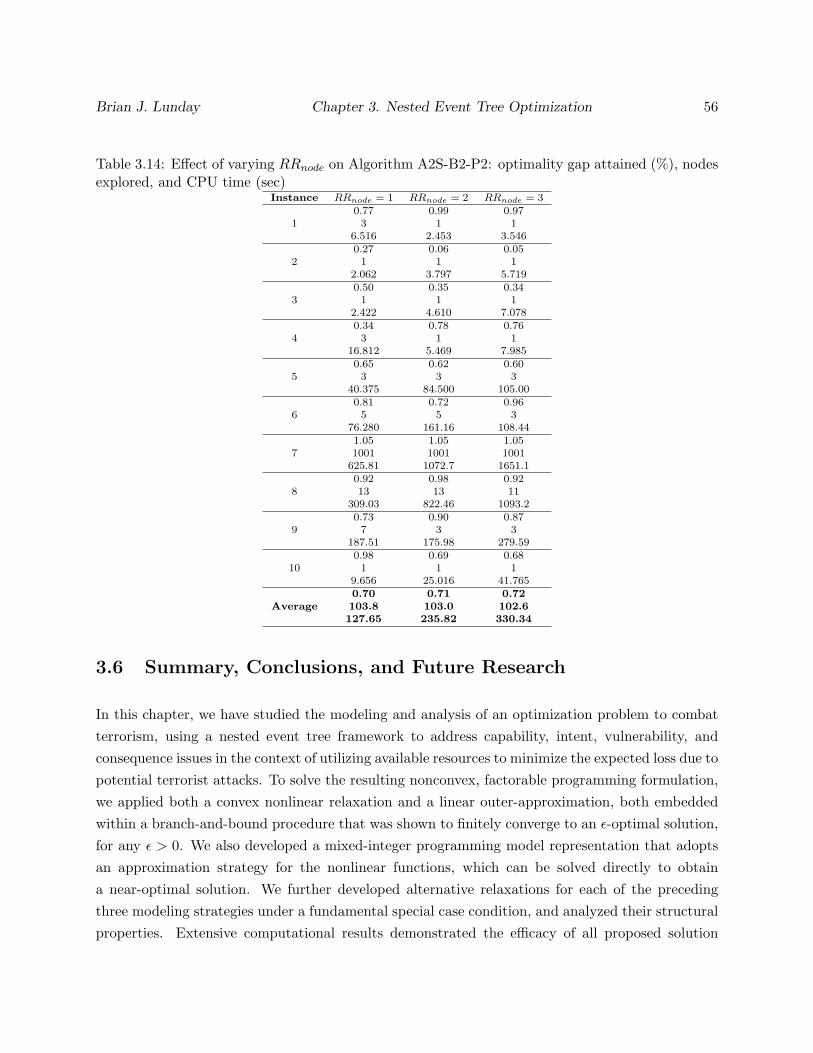
Brian J. Lunday Chapter 3. Nested Event Tree Optimization 56
Table 3.14: Effect of varying RRnode on Algorithm A2S-B2-P2: optimality gap attained (%), nodesexplored, and CPU time (sec)
Instance RRnode = 1 RRnode = 2 RRnode = 3
10.77 0.99 0.973 1 1
6.516 2.453 3.546
20.27 0.06 0.051 1 1
2.062 3.797 5.719
30.50 0.35 0.341 1 1
2.422 4.610 7.078
40.34 0.78 0.763 1 1
16.812 5.469 7.985
50.65 0.62 0.603 3 3
40.375 84.500 105.00
60.81 0.72 0.965 5 3
76.280 161.16 108.44
71.05 1.05 1.051001 1001 1001
625.81 1072.7 1651.1
80.92 0.98 0.9213 13 11
309.03 822.46 1093.2
90.73 0.90 0.877 3 3
187.51 175.98 279.59
100.98 0.69 0.681 1 1
9.656 25.016 41.765
Average0.70 0.71 0.72103.8 103.0 102.6127.65 235.82 330.34
3.6 Summary, Conclusions, and Future Research
In this chapter, we have studied the modeling and analysis of an optimization problem to combatterrorism, using a nested event tree framework to address capability, intent, vulnerability, andconsequence issues in the context of utilizing available resources to minimize the expected loss due topotential terrorist attacks. To solve the resulting nonconvex, factorable programming formulation,we applied both a convex nonlinear relaxation and a linear outer-approximation, both embeddedwithin a branch-and-bound procedure that was shown to finitely converge to an ε-optimal solution,for any ε > 0. We also developed a mixed-integer programming model representation that adoptsan approximation strategy for the nonlinear functions, which can be solved directly to obtaina near-optimal solution. We further developed alternative relaxations for each of the precedingthree modeling strategies under a fundamental special case condition, and analyzed their structuralproperties. Extensive computational results demonstrated the efficacy of all proposed solution
Brian J. Lunday Chapter 3. Nested Event Tree Optimization 57
techniques, compared to the commercial software BARON, and sensitivity analyses demonstratedthe ability to further improve algorithmic performance by varying certain key parameters.
The import of our model lies in its suitability for higher level strategic planning for resourcedeployment. In addition to optimally allocating existing resources within budgetary constraints,our model has further value for conducting what-if scenario analyses, wherein a coordinating agencycan assess the impact of adjusting budgets or resource levels, or seek to enhance effectiveness by con-sidering the adjustment of resource levels between the different capability-, intent-, vulnerability-,and consequence-related domains. A principal component in applying our model is to adequatelycalibrate the resource-probability and resource-outcome logit model parameters. We suggest thatthere is sufficient data collected within recent decades to enable such a calibration (albeit poten-tially classified and/or requiring the cooperation of strategic partners), where the nature of the logitmodels enables separable calibration steps specific to each resource type. Furthermore, such cali-bration efforts might be facilitated by simulating response functions using game-theoretic models(e.g., see Zhuang and Bier, 2007).
For future research, our model could be modified to better represent the current terror-ist threat and the complexity of international relations. The model could be expanded in scopeto account for multiple terrorist organizations and for partially aligned interests between nationsapplying resources to combat terrorism. These considerations give rise to a cooperative game,thereby requiring alternative measures of optimality or equilibrium. For larger-sized instances, thepotential need to reduce computational effort for Algorithm A3S may also merit the applicationof alternative construction techniques for piecewise linear approximations (e.g., see Vielma, et al.,2009).
Another modeling consideration is to explore alternative probability-resource relationships.One such option is the Gompertz function (Waliszewski and Konarski 2006) specified below:
pMi = e−be
−c
(α0
i−∑
s∈SMi
αsixMsi
), where b, c ∈ R+.
As the inverse of a log-log function, the Gompertz function can also be linearized using a poly-hedral outer-approximation to a convex-concave transformed function of the form pM
i = e−eqi ,maintaining the validity of Algorithms A1, A2, and A3. A comparison of the representability ofthe probability-resource relationships using such alternative functions, in addition to their effect onthe computational performance of related algorithms, is a useful endeavor for future research.
Finally, we propose the application of our model to the resource prioritization phase of theUS National Infrastructure Protection Plan (DHS 2009) in order to validate priorities among andwithin the 18 sectors of Critical Infrastructure and Key Resources (CIKR). Although the classified

Brian J. Lunday Chapter 3. Nested Event Tree Optimization 58
nature of the data, even in aggregated form, precludes addressing such a potential use here, such astudy might be of insightful value to the Department of Homeland Security, as well as its federal,state, local, and private sector partners.
Chapter 4
Network Flow Interdiction with
Resource Synergy Considerations
4.1 Introduction
In this chapter, we present our research on the network interdiction problems, as introduced inSection 1.1.2 and outlined in Section 1.2. We begin this chapter by presenting in Section 4.2, amodel formulation to minimize the maximum flow of an adversary over a network, while apply-ing multiple constrained resources and allowing for partial arc interdiction, and also consideringsuperadditive synergy between resources on each arc. Here, we consider the maximum synergyeffects to be linearly proportional to the minimum level of interdiction by any of the availableresources. We compare the ability of alternative formulations to optimally solve the problem, andconduct extensive computational tests to study the sensitivity of various measures of synergy at-tained at optimality to different problem parameters. In Section 4.3, we modify our formulationto consider concave nonlinear, and convex-concave nonlinear synergy relationships. For concavenonlinear relationships, which yield convex programs, we develop variants of an inner-linearizationprocedure and compare these to the performance of a commercial solver (SBB) designed for convexprograms, using a range of specified termination criteria. For convex-concave synergy relationships,we explore various approximation granularities and construction techniques for inner-linearizations,piecewise approximations, and outer-approximations, and then compare these against the perfor-mance of commercial solvers designed for convex (SBB) as well as nonconvex (BARON) problems.We conclude the study in Section 4.4 with a summary and recommendations for future research.
59

Brian J. Lunday Chapter 4. Network Flow Interdiction with Synergy 60
4.2 Minimize the Maximum Flow: Multiple Resources with Lin-
ear Synergy
In this section, we address the deterministic interdiction of a capacitated network having a givensource and terminus node, by utilizing multiple interdiction resources with arc-wise superadditivelinear synergy to minimize the maximum flow through the network.
4.2.1 Model Development
To facilitate our model formulation, we begin by introducing notation for the sets of nodes, arcs,and interdiction resources, as follows:Set Notation:
• N , set of nodes (indexed by i) in the network, with source s and terminus t.
• A, set of directed arcs (i, j) in the network, i, j ∈ N, i 6= j.
• G[N,A]: the underlying network.
• K, set of resource types (indexed by k) for interdiction (detection), with K = |K|.
Decision Variables:
• pijk: the percentage of capacity reduction for arc (i, j) as affected by the application of inter-dictor resource type k. (Our model allows for partial interdiction to allow for the convolutionof different types of resources, enabling the presence of superadditive synergy.)
• xij : the amount of non-negative evader flow on arc (i, j).
• σij : the additional contribution due to synergy on arc (i, j) due to the interaction of allresources, k ∈ K.
• z: the maximal flow through the network.
Parameters:
• uij : uninterdicted flow capacity for arc (i, j).
• cijk: the cost (in resource units) to completely interdict arc (i, j) using resource k.
• Rk: the maximum amount of units of resource k available for interdiction.

Brian J. Lunday Chapter 4. Network Flow Interdiction with Synergy 61
• f : a linear synergy factor representing the additional (maximum) percentage of interdictiondue to cooperation between resources (e.g., if cooperation produces (up to) a 10% increase ineffectiveness based on the minimum interdiction due to the different resources, then f = 0.1).
Accordingly, we propose the following model formulation for the network interdiction problem withmultiple resources and linear synergy (NIP-MRLS):
NIP-MRLS: minp,σ
maxx
z
subject to∑
j:(i,j)∈A
xij −∑
j:(j,i)∈A
xji =
z if i = s
0 if i 6= s, t
−z if i = t
, ∀ i ∈ N, (4.1)
∑(i,j)∈A
cijk pijk ≤ Rk, ∀ k ∈ K, (4.2)
xij ≤ uij(1−∑k∈K
pijk − σij), ∀ (i, j) ∈ A, (4.3)∑k∈K
pijk + σij ≤ 1, ∀ (i, j) ∈ A, (4.4)
σij ≤ f pijk, ∀ (i, j) ∈ A, k ∈ K, (4.5)
(xij , σij) ≥ 0, ∀ (i, j) ∈ A. (4.6)
This formulation differs from Wood’s (1993) consideration of multiple resources in the context ofbinary (yes–no) interdiction, where either some specified units are required for each resource, or aspecified allocation for only one resource is required, to completely interdict any given arc; suchformulations therefore do not account for partial interdiction or any synergistic effect. Constraint(4.1) represents the conservation of flow at each node in the network, where z denotes the netflow between the source, s, and the terminus node, t. Constraint (4.2) enforces the budget foreach resource type, and Constraint (4.3) bounds the arc flows based on interdicted capacities.The resultant interdicted capacities are non-negative by Constraint (4.4), while Constraint (4.5)bounds the amount of synergy attained on any arc. The form of superadditive synergy we considerin Constraint (4.5) requires the presence of all resource types, and is limited by the resource thathas the least interdictive effect on arc (i, j). Henceforth, the term synergy refers to this type ofsuperadditive synergy, though we do apply different functional forms for the synergistic effectsin Section 4.3. Finally, Constraint (4.6) imposes non-negativity restrictions on the arc flows andsynergy levels.
Remark 4.1. To further explain the concept of synergy, consider the case of K resources withequal interdictions on some arc (i, j), and where all K resources must be allocated in order to obtainany synergy. In this case, an efficient solution will minimize the imbalance of allocated resources
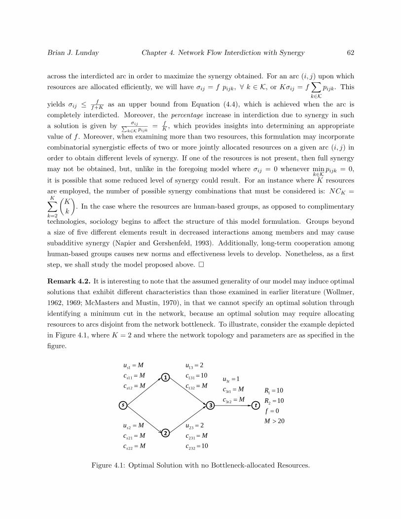
Brian J. Lunday Chapter 4. Network Flow Interdiction with Synergy 62
across the interdicted arc in order to maximize the synergy obtained. For an arc (i, j) upon whichresources are allocated efficiently, we will have σij = f pijk, ∀ k ∈ K, or Kσij = f
∑k∈K
pijk. This
yields σij ≤ ff+K as an upper bound from Equation (4.4), which is achieved when the arc is
completely interdicted. Moreover, the percentage increase in interdiction due to synergy in sucha solution is given by σij∑
k∈K pijk= f
K , which provides insights into determining an appropriatevalue of f . Moreover, when examining more than two resources, this formulation may incorporatecombinatorial synergistic effects of two or more jointly allocated resources on a given arc (i, j) inorder to obtain different levels of synergy. If one of the resources is not present, then full synergymay not be obtained, but, unlike in the foregoing model where σij = 0 whenever min
k∈Kpijk = 0,
it is possible that some reduced level of synergy could result. For an instance where K resourcesare employed, the number of possible synergy combinations that must be considered is: NCK =K∑
k=2
(K
k
). In the case where the resources are human-based groups, as opposed to complimentary
technologies, sociology begins to affect the structure of this model formulation. Groups beyonda size of five different elements result in decreased interactions among members and may causesubadditive synergy (Napier and Gershenfeld, 1993). Additionally, long-term cooperation amonghuman-based groups causes new norms and effectiveness levels to develop. Nonetheless, as a firststep, we shall study the model proposed above.
Remark 4.2. It is interesting to note that the assumed generality of our model may induce optimalsolutions that exhibit different characteristics than those examined in earlier literature (Wollmer,1962, 1969; McMasters and Mustin, 1970), in that we cannot specify an optimal solution throughidentifying a minimum cut in the network, because an optimal solution may require allocatingresources to arcs disjoint from the network bottleneck. To illustrate, consider the example depictedin Figure 4.1, where K = 2 and where the network topology and parameters are as specified in thefigure.
s t
1
2
3
Mc
Mc
Mu
s
s
s
12
11
1
Mc
Mc
Mu
s
s
s
22
21
2
Mc
c
u
132
131
13
10
2
10
2
232
231
23
c
Mc
u
Mc
Mc
u
t
t
t
23
13
3 1
20
0
10
10
2
1
M
f
R
R
Figure 4.1: Optimal Solution with no Bottleneck-allocated Resources.
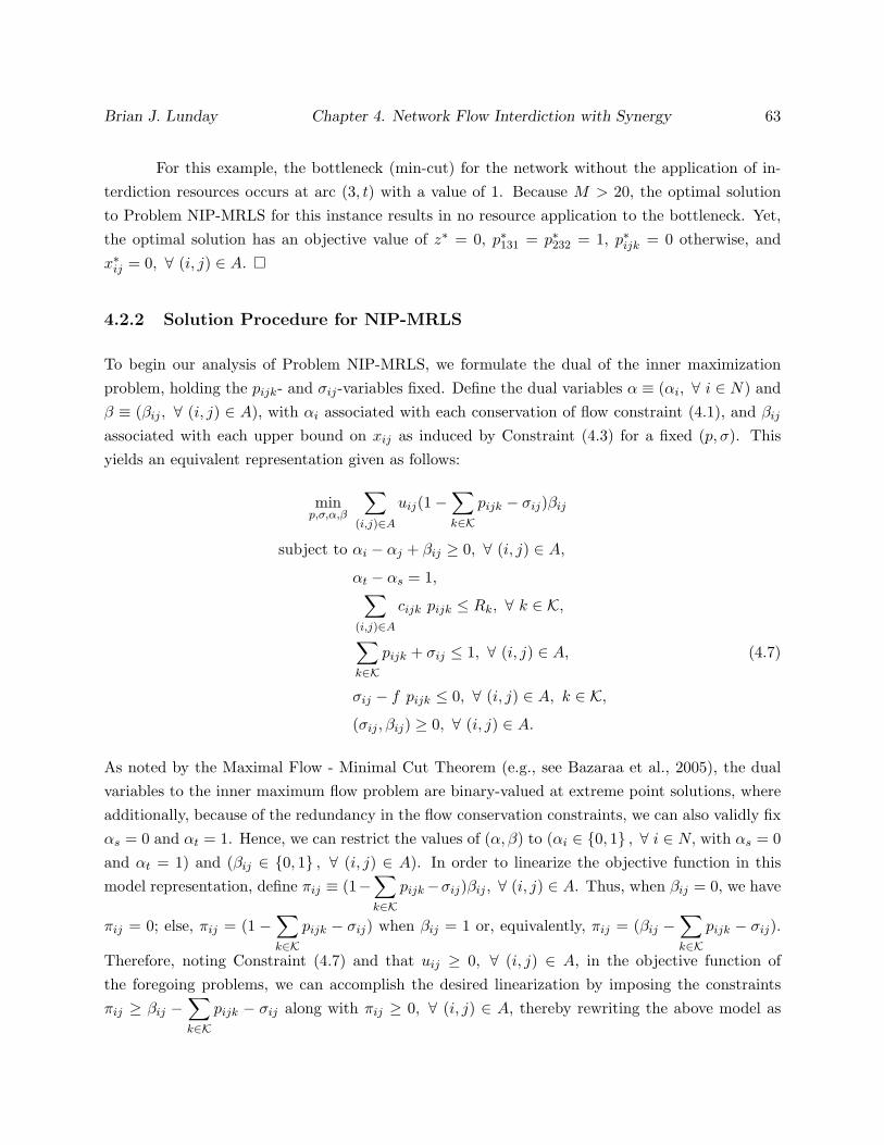
Brian J. Lunday Chapter 4. Network Flow Interdiction with Synergy 63
For this example, the bottleneck (min-cut) for the network without the application of in-terdiction resources occurs at arc (3, t) with a value of 1. Because M > 20, the optimal solutionto Problem NIP-MRLS for this instance results in no resource application to the bottleneck. Yet,the optimal solution has an objective value of z∗ = 0, p∗131 = p∗232 = 1, p∗ijk = 0 otherwise, andx∗ij = 0, ∀ (i, j) ∈ A.
4.2.2 Solution Procedure for NIP-MRLS
To begin our analysis of Problem NIP-MRLS, we formulate the dual of the inner maximizationproblem, holding the pijk- and σij-variables fixed. Define the dual variables α ≡ (αi, ∀ i ∈ N) andβ ≡ (βij , ∀ (i, j) ∈ A), with αi associated with each conservation of flow constraint (4.1), and βij
associated with each upper bound on xij as induced by Constraint (4.3) for a fixed (p, σ). Thisyields an equivalent representation given as follows:
minp,σ,α,β
∑(i,j)∈A
uij(1−∑k∈K
pijk − σij)βij
subject to αi − αj + βij ≥ 0, ∀ (i, j) ∈ A,
αt − αs = 1,∑(i,j)∈A
cijk pijk ≤ Rk, ∀ k ∈ K,∑k∈K
pijk + σij ≤ 1, ∀ (i, j) ∈ A, (4.7)
σij − f pijk ≤ 0, ∀ (i, j) ∈ A, k ∈ K,
(σij , βij) ≥ 0, ∀ (i, j) ∈ A.
As noted by the Maximal Flow - Minimal Cut Theorem (e.g., see Bazaraa et al., 2005), the dualvariables to the inner maximum flow problem are binary-valued at extreme point solutions, whereadditionally, because of the redundancy in the flow conservation constraints, we can also validly fixαs = 0 and αt = 1. Hence, we can restrict the values of (α, β) to (αi ∈ 0, 1 , ∀ i ∈ N, with αs = 0and αt = 1) and (βij ∈ 0, 1 , ∀ (i, j) ∈ A). In order to linearize the objective function in thismodel representation, define πij ≡ (1−
∑k∈K
pijk−σij)βij , ∀ (i, j) ∈ A. Thus, when βij = 0, we have
πij = 0; else, πij = (1 −∑k∈K
pijk − σij) when βij = 1 or, equivalently, πij = (βij −∑k∈K
pijk − σij).
Therefore, noting Constraint (4.7) and that uij ≥ 0, ∀ (i, j) ∈ A, in the objective function ofthe foregoing problems, we can accomplish the desired linearization by imposing the constraintsπij ≥ βij −
∑k∈K
pijk − σij along with πij ≥ 0, ∀ (i, j) ∈ A, thereby rewriting the above model as

Brian J. Lunday Chapter 4. Network Flow Interdiction with Synergy 64
follows:
P1: minp,σ,α,β,π
∑(i,j)∈A
uijπij
subject to αi − αj + βij ≥ 0, ∀ (i, j) ∈ A, (4.8)∑(i,j)∈A
cijk pijk ≤ Rk, ∀ k ∈ K,∑k∈K
pijk + σij ≤ 1, ∀ (i, j) ∈ A,
σij − f pijk ≤ 0, ∀ (i, j) ∈ A, k ∈ K,
πij +∑k∈K
pijk + σij − βij ≥ 0, ∀ (i, j) ∈ A, (4.9)
(σij , πij) ≥ 0, ∀ (i, j) ∈ A,
αi ∈ 0, 1 , ∀ i ∈ N, with αs = 0 and αt = 1,
βij ∈ 0, 1 , ∀ (i, j) ∈ A. (4.10)
Now, consider the following related formulation P2, which appropriately eliminates the β-variablesin a manner that is established in Proposition 4.1 below to yield an equivalent alternative to solvingModel P1.
P2: minp,σ,α,π
∑(i,j)∈A
uijπij (4.11)
subject to αi − αj + πij +∑k∈K
pijk + σij ≥ 0, ∀ (i, j) ∈ A, (4.12)∑(i,j)∈A
cijk pijk ≤ Rk, ∀ k ∈ K,∑k∈K
pijk + σij ≤ 1, ∀ (i, j) ∈ A,
σij − f pijk ≤ 0, ∀ (i, j) ∈ A, k ∈ K,
(σij , πij) ≥ 0, ∀ (i, j) ∈ A,
αi ∈ 0, 1 , ∀ i ∈ N, with αs = 0 and αt = 1. (4.13)
Proposition 4.1. Any optimal solution to Problem P2 solves Problem P1.
Proof. First of all, note that P2 is a relaxation of P1 in which (4.10) is omitted, and then βij iseliminated by using (4.8) and (4.9), ∀ (i, j) ∈ A (as in Fourier-Motzkin elimination). Hence, it issufficient to show that any optimal solution (p∗, s∗, α∗, π∗) to Problem P2 yields a correspondingfeasible solution (p∗, s∗, α∗, π∗, β∗) to Problem P1 having the same objective value. Given such an
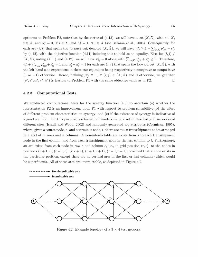
Brian J. Lunday Chapter 4. Network Flow Interdiction with Synergy 65
optimum to Problem P2, note that by the virtue of (4.13), we will have a cut [X, X], with s ∈ X,t ∈ X, and α∗i = 0, ∀ i ∈ X, and α∗i = 1, ∀ i ∈ X (see Bazaraa et al., 2005). Consequently, foreach arc (i, j) that spans the forward cut, denoted (X, X), we will have π∗ij ≥ 1−
∑k∈K p
∗ijk − s∗ij
by (4.12), with the objective function (4.11) inducing this to hold as an equality. Else, for (i, j) /∈(X, X), noting (4.11) and (4.12), we will have π∗ij = 0 along with
∑k∈K p
∗ijk + s∗ij ≥ 0. Therefore,
π∗ij +∑
k∈K p∗ijk +s∗ij = 1 and α∗j −α∗i = 1 for each arc (i, j) that spans the forward cut (X, X), with
the left-hand side expressions in these two equations being respectively nonnegative or nonpositive(0 or −1) otherwise. Hence, defining β∗ij ≡ 1, ∀ (i, j) ∈ (X, X) and 0 otherwise, we get that(p∗, s∗, α∗, π∗, β∗) is feasible to Problem P1 with the same objective value as in P2.
4.2.3 Computational Tests
We conducted computational tests for the synergy function (4.5) to ascertain (a) whether therepresentation P2 is an improvement upon P1 with respect to problem solvability; (b) the effectof different problem characteristics on synergy; and (c) if the existence of synergy is indicative ofa good solution. For this purpose, we tested our models using a set of directed grid networks ofdifferent sizes (Israeli and Wood, 2002) and randomly generated arc attributes (Cormican, 1995),where, given a source node, s, and a terminus node, t, there are m×n transshipment nodes arrangedin a grid of m rows and n columns. A non-interdictable arc exists from s to each transshipmentnode in the first column, and from each transshipment node in the last column to t. Furthermore,an arc exists from each node in row r and column c, i.e., in grid position (r, c), to the nodes inpositions (r + 1, c), (r − 1, c), (r, c+ 1), (r + 1, c+ 1), (r − 1, c+ 1), provided that a node exists inthe particular position, except there are no vertical arcs in the first or last columns (which wouldbe superfluous). All of these arcs are interdictable, as depicted in Figure 4.2.
Non-interdictable arcs
Interdictable arcs
s t
Figure 4.2: Example topology of a 3 × 4 test network.

Brian J. Lunday Chapter 4. Network Flow Interdiction with Synergy 66
The basic data for each network are as follows: (a) m and n: hence, there are a =(n − 2)(5m − 4) + 3m − 2 interdictable arcs and 2m non-interdictable arcs; (b) maximum arccapacity range, uij : [10, 100], uniformly distributed in increments of 10; (c) interdiction cost, cijk:[10, 100], uniformly distributed in increments of 10; (d) resource availability, Rk: [10, 50m], uni-formly distributed in increments of 10; and (e) synergy factor, f : [0, 0.5], uniformly distributed inincrements of 0.05.
Remark 4.3. We have assumed that there exists no relationship between the parameters uij
and cijk, ∀ (i, j) ∈ A, k ∈ K. Depending on the network interdiction application, we may actuallyexpect a relationship between these parameters, but the nature of that relationship is not necessarilyconsistent for all applications. Intuitively, one might expect a positive correlation between uij andcijk, ∀ (i, j) ∈ A, k ∈ K. A network arc with greater capacity should theoretically be moredifficult for a given resource to interdict completely. Hence, as uij increases, cijk increases for allk ∈ K. However, the nature of this relationship is application-dependent and other cases do exist.Consider an instance in which a nation wishes to interdict all traffic transiting their border. Itwill require the same amount of a given resource type to interdict traffic on a two-lane highway asalong a two-lane country road, even though the former has a higher capacity for traffic flow due tocharacteristics such as roadway design and speed limit. For this example, we expect no correlationbetween uij and cijk. A negative correlation may also exist, as for example in the case of a rural roadthat is sufficiently remote so that it requires more resources for interdiction than a highway. Thisrelationship would occur in applications where the cost of arc interdiction incorporates resourcesdedicated to both physically interdict the arc and logistically support the operation.
4.2.3.1 Comparison of Model Formulations P1 and P2
We tested and compared the formulations P1 and P2 with respect to how quickly the solver AMPL-CPLEX 11.1 converges to an optimal solution over the set of test problems identified in Table 4.1.For this experiment, we refer to networks as being small, medium, or large, as indicated in Column1, based on the number of arcs, a, as specified in Column 3. For each of the 15 cases displayedin Table 4.1, we generated 100 random instances and solved them using AMPL-CPLEX 11.1 on acomputer with an Intel 4.40 GHz Xeon Processor and 1.5 GB of RAM. The results obtained arereported in Table 4.2.

Brian J. Lunday Chapter 4. Network Flow Interdiction with Synergy 67
Table 4.1: Test problems for comparing Models P1 and P2.Network Problem m× n a
Small (a < 500), with (m = n)
1 4 × 4 422 5 × 5 763 6 × 6 1204 7 × 7 1745 8 × 8 2386 9 × 9 3127 10 × 10 396
Medium (500 < a < 1500), with (m 6= n)
8 10 × 15 6269 15 × 10 61110 15 × 20 132111 20 × 15 1306
Large (a > 1500), with (m = n)
12 20 × 20 178613 30 × 30 417614 40 × 40 756615 50 × 50 11,956
Table 4.2: Comparison of Models P1 and P2.Problem Structure Average CPLEX Solve Time
Avg MIP Simplex IterationsAvg B&B
Problem (P2/P1 Ratios) (CPU Seconds) NodesDec. Vars. Constraints P1 P2 P2/P1 P1 P2 P2/P1 P1 P2
1 0.8158 0.7640 0.02170 0.01405 0.6475 218.35 195.82 0.8968 0.01 0.002 0.8427 0.7871 0.04797 0.03168 0.6604 342.38 311.48 0.9097 0.02 0.043 0.8633 0.8068 0.09206 0.05698 0.6189 520.01 448.50 0.8625 0.02 0.004 0.8794 0.8234 0.20154 0.10380 0.5150 721.96 621.38 0.8607 0.10 0.195 0.8922 0.8374 0.51547 0.24209 0.4696 1058.5 891.44 0.8425 0.08 0.156 0.9026 0.8495 0.58374 0.34007 0.5826 1313.7 1090.14 0.8298 0.07 0.207 0.9112 0.8599 0.71057 0.43094 0.6065 1605.24 1336.74 0.8327 0.05 0.15
8 0.9183 0.8689 4.71780 2.60642 0.5525 2345.52 1897.96 0.8092 0.17 0.169 0.9245 0.8770 4.31911 2.23898 0.5184 2540.87 2074.61 0.8165 0.12 0.2110 0.9297 0.8840 17.44036 7.50472 0.4303 5343.76 4139.23 0.7746 0.73 0.5911 0.9343 0.8904 10.76644 6.87656 0.6387 5517.45 4388.42 0.7954 0.70 0.69
12 0.9384 0.8960 21.54643 13.19334 0.6123 7437.58 5763.37 0.7749 0.79 0.7513 0.9419 0.9011 81.92375 54.21130 0.6617 17521.1 13419.78 0.7659 0.78 0.8414 0.9451 0.9057 351.79709 143.08970 0.4067 32217.14 24365.89 0.7563 1.39 1.6615 0.9479 0.9100 496.70693 355.44806 0.7156 51080.93 38912.81 0.7618 1.56 1.66
Average = 0.5758 Average = 0.8193
Over the set of test problems, Model P2 resulted in a 43.42% reduction in solution time,on average, over Model P1. This solution time improvement occurs despite a weakly correlatedreduction in the number of MIP Simplex Iterations by 18.07%.
4.2.3.2 Sensitivity Analyses and the Impact of Synergy
We conducted extensive sensitivity analyses for the two-resource problem to study the relationshipsbetween the correlation of the cijk-values, herein denoted rcosts, the problem size, and the linearsynergy factor (f), as well as the impact of considering synergy. The major observations aresummarized below, and detailed in the succeeding sections 4.2.3.2.1–4.2.3.2.3.

Brian J. Lunday Chapter 4. Network Flow Interdiction with Synergy 68
(a) A positive correlation exists between rcosts, positive-valued rcosts, or negative-valued rcosts
and various synergy metrics examined at optimality (e.g., 100 mink∈K
∑(i,j)∈A
(σijcijk
K
)Rk
), with
the correlation being much stronger when rcosts > 0 ([0.20, 0.27]), thereby indicating thatcorrelated costs tend to favor optimal solutions with co-located resources and higher synergylevels.
(b) An increase in the f -value increases the magnitude of the correlation between rcosts and thesynergy metrics (e.g., the correlation using the metric in (a) above was 0.0563 at f = 0.05,but 0.1323 at f = 0.5).
(c) The effect of considering synergy accentuates with an increase in f , with an average of 1.25%improvement in disrupted flow and a corresponding 14.98% reduction in the net flow forf = 0.5, compared to the results without synergy.
4.2.3.2.1 Instance Parameters and Synergy. We next examined the sample test problemswith respect to three measures: (a) the correlation of the cijk-values between the two resources, re-ferred to henceforth as rcosts; (b) the synergy scale factor f ; and (c) the percentage of resources Rk
attributed to synergy-producing interdictions. The first measure is assessed by directly computingthe correlation coefficient, and the second measure relates to the synergy restricting model param-eter f . For the third measure, note that if we define pijk = pijk +λijkσij ,∀ (i, j) ∈ A, k ∈ K, where∑
k∈K λijk = 1, ∀ (i, j) ∈ A, and λ ≥ 0, then pij =∑
k∈K pijk. Hence, the effective interdiction isgiven by p, but with only the pijk-component actually consuming the resources Rk, so that the netpercentage boost in resources attributed to synergy is given by 100
[∑(i,j)∈A cijkλijkσij
]/Rk, ∀ k ∈
K. Furthermore, if we assume that the synergy on arc (i, j) is due uniformly with respect to the Kresources, then we get λijk = 1/K, ∀ (i, j) ∈ A, k ∈ K. Accordingly, we compute the minimum,average, and maximum percentage of resources attributed to synergy as follows:
SUk-MIN = 100min
k∈K
∑(i,j)∈A
(σijcijk
K
)Rk
,
SUk-AVG =
100K
∑k∈K
(∑(i,j)∈A
(σijcijk
K
)Rk
),
SUk-MAX = 100max
k∈K
∑(i,j)∈A
(σijcijk
K
)Rk
.
An alternative interpretation is to apportion ‘credit’ for synergy in proportion to each resource’srelative interdiction of the arc. That is, we can take λijk = pijk∑
k∈K pijk, ∀ k ∈ K, for each (i, j) ∈
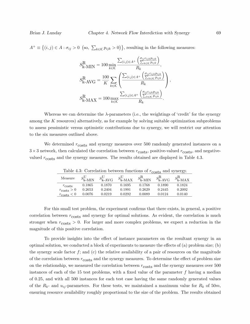
Brian J. Lunday Chapter 4. Network Flow Interdiction with Synergy 69
A+ ≡(i, j) ∈ A : σij > 0
(so,
∑k∈K pijk > 0
), resulting in the following measures:
SRk-MIN = 100min
k∈K
∑(i,j)∈A+
(σijcijkpijk∑
k∈K pijk
)Rk
,
SRk-AVG =
100K
∑k∈K
∑(i,j)∈A+
(σijcijkpijk∑
k∈K pijk
)Rk
,
SRk-MAX = 100max
k∈K
∑(i,j)∈A+
(σijcijkpijk∑
k∈K pijk
)Rk
.
Whereas we can determine the λ-parameters (i.e., the weightings of ‘credit’ for the synergyamong the K resources) alternatively, as for example by solving suitable optimization subproblemsto assess pessimistic versus optimistic contributions due to synergy, we will restrict our attentionto the six measures outlined above.
We determined rcosts and synergy measures over 500 randomly generated instances on a3×3 network, then calculated the correlation between rcosts, positive-valued rcosts, and negative-valued rcosts and the synergy measures. The results obtained are displayed in Table 4.3.
Table 4.3: Correlation between functions of rcosts and synergy.
Measure SUk-MIN SU
k-AVG SUk-MAX SR
k-MIN SRk-AVG SR
k-MAX
rcosts 0.1865 0.1870 0.1695 0.1768 0.1890 0.1824rcosts > 0 0.2653 0.2404 0.1991 0.2629 0.2445 0.2092rcosts < 0 0.0076 0.0219 0.0292 0.0089 0.0124 0.0140
For this small test problem, the experiment confirms that there exists, in general, a positivecorrelation between rcosts and synergy for optimal solutions. As evident, the correlation is muchstronger when rcosts > 0. For larger and more complex problems, we expect a reduction in themagnitude of this positive correlation.
To provide insights into the effect of instance parameters on the resultant synergy in anoptimal solution, we conducted a block of experiments to measure the effects of (a) problem size; (b)the synergy scale factor f ; and (c) the relative availability of a pair of resources on the magnitudeof the correlation between rcosts and the synergy measures. To determine the effect of problem sizeon the relationship, we measured the correlation between rcosts and the synergy measures over 500instances of each of the 15 test problems, with a fixed value of the parameter f having a medianof 0.25, and with all 500 instances for each test case having the same randomly generated valuesof the Rk- and uij-parameters. For these tests, we maintained a maximum value for Rk of 50m,ensuring resource availability roughly proportional to the size of the problem. The results obtained

Brian J. Lunday Chapter 4. Network Flow Interdiction with Synergy 70
are displayed in Table 4.4.
Table 4.4: Correlation between rcosts and synergy over 15 test problem sizes.
Problem SUk-MIN SU
k-AVG SUk-MAX SR
k-MIN SRk-AVG SR
k-MAXrcosts
1 0.0993 0.1175 0.1232 0.1254 0.1161 0.1052 [−0.4286, 0.4730]2 0.0970 0.0985 0.0973 0.0907 0.0987 0.1028 [−0.3012, 0.3984]3 0.0757 0.0670 0.0593 0.0632 0.0684 0.0712 [−0.2168, 0.2630]4 0.0777 0.0793 0.0773 0.0656 0.0851 0.0922 [−0.2311, 0.2160]5 0.0357 0.0433 0.0486 0.0365 0.0440 0.0496 [−0.2059, 0.3792]6 0.0126 0.0174 0.0195 0.0113 0.0157 0.0177 [−0.1627, 0.1563]7 0.0291 0.0371 0.0417 0.0307 0.0351 0.0373 [−0.1639, 0.1223]
8 0.1075 0.1119 0.1120 0.1154 0.1103 0.1040 [−0.1144, 0.2414]9 0.0670 0.0660 0.0655 0.0663 0.0648 0.0644 [−0.1068, 0.1282]10 0.0723 0.0741 0.0744 0.0682 0.0747 0.0788 [−0.0747, 0.0852]11 0.0837 0.0830 0.0815 0.0800 0.0831 0.0844 [−0.0760, 0.0895]
12 0.0624 0.0662 0.0672 0.0602 0.0662 0.0684 [−0.0774, 0.0605]13 0.1056 0.1098 0.1104 0.1023 0.1098 0.1127 [−0.0484, 0.0482]14 0.0443 0.0426 0.0408 0.0460 0.0411 0.0380 [−0.0427, 0.0327]15 0.0144 0.0105 0.0078 0.0191 0.0094 0.0037 [−0.0241, 0.0242]
As expected, the range of rcosts for the randomly generated problems decreases as theproblem size increases, since the effect of an individual cij-value has a decreasing effect on rcosts,from the expected value of E (rcosts) = 0. Nevertheless, an increase in problem size, with anapproximately proportional increase in the maximum resource availability, maintains a weak, posi-tive correlation between rcosts and the synergy measures. However, there is insufficient evidence tosupport a conclusion that the correlation between rcosts and any of the synergy measures decreasesover these test problem sizes.
Next, we examined the effect of the synergy scale factor, f , on the correlation betweenrcosts and the synergy measures over 500 randomly-generated instances of the cij-parameters on a10× 10 network for each value of f ∈ 0.05, 0.1, . . . , 0.5. The maximum value for f was limited at0.5 because it implies that, with synergy, two resources effectively interdict an arc when they haveeach interdicted 40% of the arc capacity. Again, we fixed the Rk- and uij-parameters to one set ofrandomly generated values for all 500 instances. The results obtained are displayed in Table 4.5.
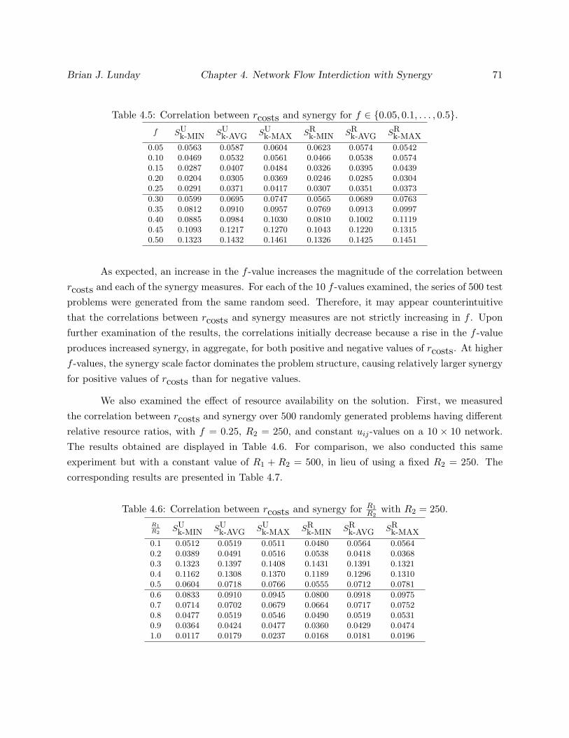
Brian J. Lunday Chapter 4. Network Flow Interdiction with Synergy 71
Table 4.5: Correlation between rcosts and synergy for f ∈ 0.05, 0.1, . . . , 0.5.f SU
k-MIN SUk-AVG SU
k-MAX SRk-MIN SR
k-AVG SRk-MAX
0.05 0.0563 0.0587 0.0604 0.0623 0.0574 0.05420.10 0.0469 0.0532 0.0561 0.0466 0.0538 0.05740.15 0.0287 0.0407 0.0484 0.0326 0.0395 0.04390.20 0.0204 0.0305 0.0369 0.0246 0.0285 0.03040.25 0.0291 0.0371 0.0417 0.0307 0.0351 0.0373
0.30 0.0599 0.0695 0.0747 0.0565 0.0689 0.07630.35 0.0812 0.0910 0.0957 0.0769 0.0913 0.09970.40 0.0885 0.0984 0.1030 0.0810 0.1002 0.11190.45 0.1093 0.1217 0.1270 0.1043 0.1220 0.13150.50 0.1323 0.1432 0.1461 0.1326 0.1425 0.1451
As expected, an increase in the f -value increases the magnitude of the correlation betweenrcosts and each of the synergy measures. For each of the 10 f -values examined, the series of 500 testproblems were generated from the same random seed. Therefore, it may appear counterintuitivethat the correlations between rcosts and synergy measures are not strictly increasing in f . Uponfurther examination of the results, the correlations initially decrease because a rise in the f -valueproduces increased synergy, in aggregate, for both positive and negative values of rcosts. At higherf -values, the synergy scale factor dominates the problem structure, causing relatively larger synergyfor positive values of rcosts than for negative values.
We also examined the effect of resource availability on the solution. First, we measuredthe correlation between rcosts and synergy over 500 randomly generated problems having differentrelative resource ratios, with f = 0.25, R2 = 250, and constant uij-values on a 10 × 10 network.The results obtained are displayed in Table 4.6. For comparison, we also conducted this sameexperiment but with a constant value of R1 + R2 = 500, in lieu of using a fixed R2 = 250. Thecorresponding results are presented in Table 4.7.
Table 4.6: Correlation between rcosts and synergy for R1R2
with R2 = 250.R1R2
SUk-MIN SU
k-AVG SUk-MAX SR
k-MIN SRk-AVG SR
k-MAX
0.1 0.0512 0.0519 0.0511 0.0480 0.0564 0.05640.2 0.0389 0.0491 0.0516 0.0538 0.0418 0.03680.3 0.1323 0.1397 0.1408 0.1431 0.1391 0.13210.4 0.1162 0.1308 0.1370 0.1189 0.1296 0.13100.5 0.0604 0.0718 0.0766 0.0555 0.0712 0.0781
0.6 0.0833 0.0910 0.0945 0.0800 0.0918 0.09750.7 0.0714 0.0702 0.0679 0.0664 0.0717 0.07520.8 0.0477 0.0519 0.0546 0.0490 0.0519 0.05310.9 0.0364 0.0424 0.0477 0.0360 0.0429 0.04741.0 0.0117 0.0179 0.0237 0.0168 0.0181 0.0196
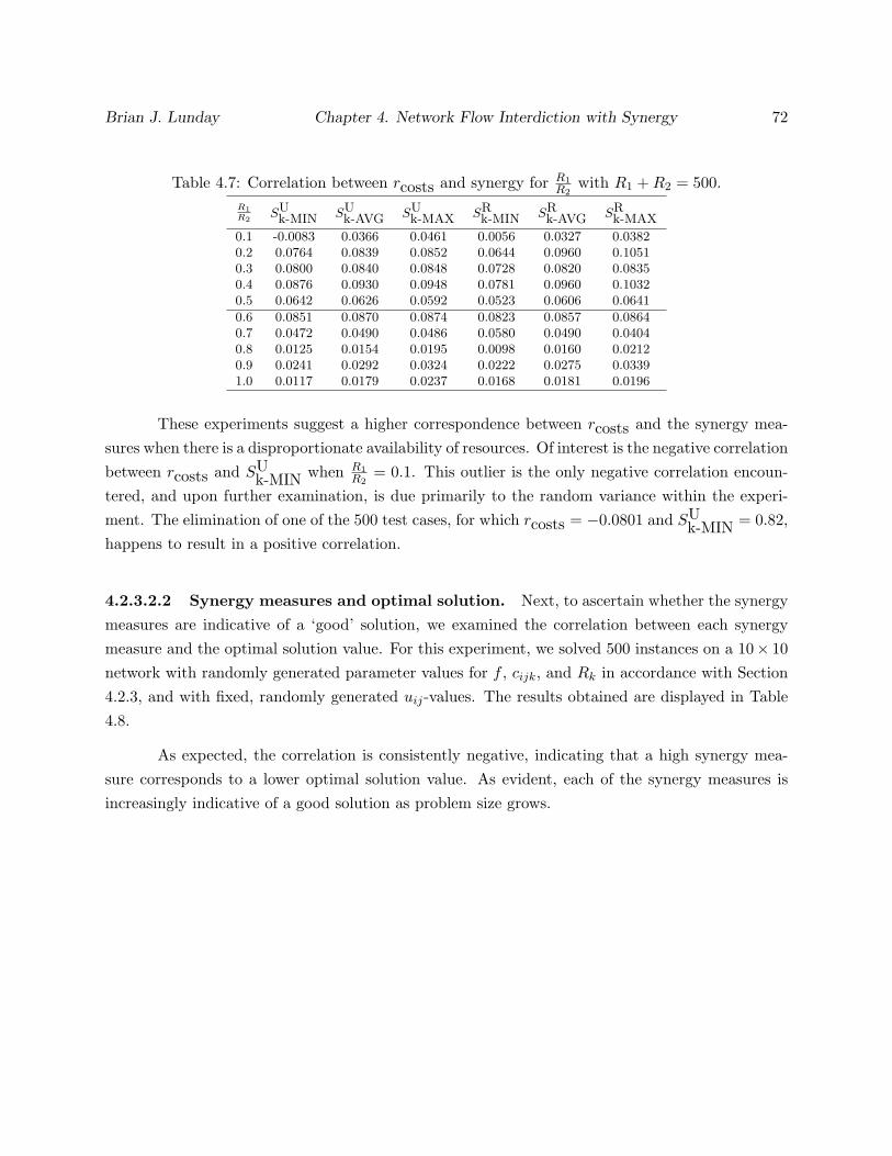
Brian J. Lunday Chapter 4. Network Flow Interdiction with Synergy 72
Table 4.7: Correlation between rcosts and synergy for R1R2
with R1 +R2 = 500.R1R2
SUk-MIN SU
k-AVG SUk-MAX SR
k-MIN SRk-AVG SR
k-MAX
0.1 -0.0083 0.0366 0.0461 0.0056 0.0327 0.03820.2 0.0764 0.0839 0.0852 0.0644 0.0960 0.10510.3 0.0800 0.0840 0.0848 0.0728 0.0820 0.08350.4 0.0876 0.0930 0.0948 0.0781 0.0960 0.10320.5 0.0642 0.0626 0.0592 0.0523 0.0606 0.0641
0.6 0.0851 0.0870 0.0874 0.0823 0.0857 0.08640.7 0.0472 0.0490 0.0486 0.0580 0.0490 0.04040.8 0.0125 0.0154 0.0195 0.0098 0.0160 0.02120.9 0.0241 0.0292 0.0324 0.0222 0.0275 0.03391.0 0.0117 0.0179 0.0237 0.0168 0.0181 0.0196
These experiments suggest a higher correspondence between rcosts and the synergy mea-sures when there is a disproportionate availability of resources. Of interest is the negative correlationbetween rcosts and SU
k-MIN when R1R2
= 0.1. This outlier is the only negative correlation encoun-tered, and upon further examination, is due primarily to the random variance within the experi-ment. The elimination of one of the 500 test cases, for which rcosts = −0.0801 and SU
k-MIN = 0.82,happens to result in a positive correlation.
4.2.3.2.2 Synergy measures and optimal solution. Next, to ascertain whether the synergymeasures are indicative of a ‘good’ solution, we examined the correlation between each synergymeasure and the optimal solution value. For this experiment, we solved 500 instances on a 10× 10network with randomly generated parameter values for f , cijk, and Rk in accordance with Section4.2.3, and with fixed, randomly generated uij-values. The results obtained are displayed in Table4.8.
As expected, the correlation is consistently negative, indicating that a high synergy mea-sure corresponds to a lower optimal solution value. As evident, each of the synergy measures isincreasingly indicative of a good solution as problem size grows.

Brian J. Lunday Chapter 4. Network Flow Interdiction with Synergy 73
Table 4.8: Correlation between synergy measures and the optimal solution values, with fixed uij-parameters.
Problem SUk-MIN SU
k-AVG SUk-MAX SR
k-MIN SRk-AVG SR
k-MAX
1 -0.1852 -0.1204 -0.0751 -0.1798 -0.1187 -0.07452 -0.2767 -0.1925 -0.1275 -0.2752 -0.1952 -0.13183 -0.2141 -0.0951 -0.0178 -0.2137 -0.1038 -0.02924 -0.2876 -0.2198 -0.1618 -0.2862 -0.2246 -0.17045 -0.3186 -0.2126 -0.1286 -0.3190 -0.2197 -0.13976 -0.2943 -0.1669 -0.0765 -0.2908 -0.1705 -0.08337 -0.2404 -0.1483 -0.0838 -0.2429 -0.1540 -0.0900
8 -0.2739 -0.1785 -0.1098 -0.2768 -0.1830 -0.11529 -0.3805 -0.2646 -0.1681 -0.3808 -0.2714 -0.178410 -0.3303 -0.2208 -0.1335 -0.3331 -0.2265 -0.139511 -0.3892 -0.2436 -0.1352 -0.3870 -0.2458 -0.1395
12 -0.3404 -0.1887 -0.0793 -0.3385 -0.1922 -0.084613 -0.3894 -0.2623 -0.1621 -0.3923 -0.2643 -0.163914 -0.3914 -0.2620 -0.1568 -0.3912 -0.2632 -0.158915 -0.3808 -0.2888 -0.2049 -0.3837 -0.2924 -0.2091
4.2.3.2.3 Impact of Synergy. Before proceeding to consider models that incorporate non-linear synergy effects, it is important to examine the overall impact of considering synergy. Wetherefore examined the non-interdicted maximum flow, denoted MFP; the maximum interdictedflow without synergy, denoted NIP-MR, when f = 0 for NIP-MRLS; and the maximum interdictedflow with linear synergy (Model P2) for any given network, with respective optimal solution valuesZMFP, ZNIP-MR, and ZP2, where ZP2 ≤ ZNIP-MR ≤ ZMFP. We then computed the followingmeasures of performance:
DI = 100ZNIP-MR − ZP2ZMFP − ZNIP-MR
,
SV R = 100ZNIP-MR − ZP2
ZNIP-MR.
Solution Value Reduction (SV R) calculates the relative percentage decrease in optimalsolution values for Model P2 compared to Model NIP-MR, whereas Disruption Improvement (DI)measures the relative percentage increase in the amount of flow that is prevented from travelingthrough the network when synergy is considered. We will have DI ≤ (100 f) (the numerator of DIrepresents the additional amount of flow interdicted due to synergy, which is bounded by “f× theamount of flow interdicted without synergy”, where the amount of flow interdicted without synergyis represented by the denominator of DI). However, determining the average impact under bothmeasures may provide insights into the potential effects of applying heuristics in the next section,in contrast to using algorithms that guarantee an optimal solution.
First, we examined the effect of considering synergy using both measures over 100 randomly-

Brian J. Lunday Chapter 4. Network Flow Interdiction with Synergy 74
generated instances for each of the 15 test problem sizes, with a fixed value for the f -parameterhaving a median of 0.25. Once more, we maintained a maximum value for Rk of 50m, ensuring aresource availability that is roughly proportional to the size of the problem. The results obtainedare displayed in Table 4.9.
Table 4.9: Effect of considering synergy over 15 test problem sizes.Problem Average DI(%) Average SV R(%)
1 0.6012 5.12462 0.5381 5.71333 0.5290 5.18184 0.5118 5.72455 0.4169 5.12516 0.4876 5.97547 0.3822 5.9497
8 0.3996 5.09559 0.3576 4.041810 0.4103 6.254511 0.3422 5.3218
12 0.3581 4.729313 0.3285 3.941714 0.2948 4.782315 0.3392 3.6229
We note that, although the average disruption improvement generally decreases with prob-lem size, the average reduction in the optimal solution value when incorporating the effect of synergyremains significant, roughly 3-7%. For the medium-sized problems having asymmetric networks,the effect of synergy is greater for the same number of nodes when m < n. Beyond demonstratingthe effect of synergy, the maximum flow value reductions displayed in Table 4.9 prompt the selec-tion of optimality tolerances when considering heuristics for more complex, non-linear formulationsin the following section.
Next, we examined the effect of considering synergy on both the amount of flow interdictedand the optimal solution value over 100 randomly-generated instances of a 10 × 10 network foreach value of f ∈ 0.05, 0.1, . . . , 0.5 . (As before, the maximum value for f was limited at 0.5.)The results obtained are displayed in Table 4.10, which quantitatively confirms the intuition thatthe effect of considering synergy accentuates with an increase in f . Moreover, this too providesguidelines on selecting optimality tolerances in the following section.

Brian J. Lunday Chapter 4. Network Flow Interdiction with Synergy 75
Table 4.10: Effect of considering synergy for f ∈ 0.05, 0.1, . . . , 0.5.f Average DI(%) Average SV R(%)
0.05 0.0400 0.95830.10 0.0909 2.31710.15 0.1586 3.21440.20 0.2586 4.44380.25 0.3822 5.9497
0.30 0.5273 7.48990.35 0.6924 9.20170.40 0.8704 11.03360.45 1.0606 13.05870.50 1.2534 14.9808
4.3 Minimize the Maximum Flow: Multiple Resources with Non-
linear Synergy
In this section, we consider two types of nonlinear relationships for synergy, respectively resulting inconvex and nonconvex programs. We then develop and test solution procedures for each formulationand compare their performance to commercial optimization software.
4.3.1 Nonlinear Synergy with Concave Synergy Function
For this case, we study the following limiting function for synergy (see Figure 4.3):
σij ≤ g(1− e−10 pijk
), ∀ (i, j) ∈ A, k ∈ K, with 0 ≤ g ≤ 0.2, (4.14)
where σij = 0 for arc (i, j) whenever pijk = 0 for any k, and σij ≤ g, ∀ (i, j) ∈ A. We impose anupper bound of g ≤ 0.2 to ensure, as before, that complete interdiction of an arc with maximumsynergy benefit requires at least 80% interdiction without synergy. The justification to apply thistype of synergy function derives from the philosophy that, whereas the simultaneous applicationof resources might return positive benefits, the marginal return on investment might decrease withadditional commitments of resources. Of course, a variety of functions could be used to obtainsuch a concave structure, all of which result in a convex problem. For example, we could useσij ≤ 0.6 ln(1+pijk), ∀ (i, j) ∈ A, k ∈ K, although this function has less curvature over the domainof interest.
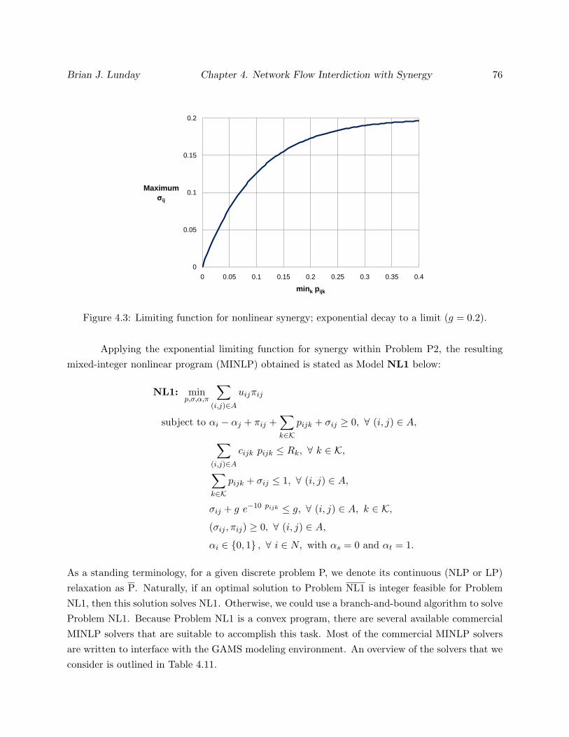
Brian J. Lunday Chapter 4. Network Flow Interdiction with Synergy 76
0
0.05
0.1
0.15
0.2
0 0.05 0.1 0.15 0.2 0.25 0.3 0.35 0.4
Maximum
ij
mink pijk
Figure 4.3: Limiting function for nonlinear synergy; exponential decay to a limit (g = 0.2).
Applying the exponential limiting function for synergy within Problem P2, the resultingmixed-integer nonlinear program (MINLP) obtained is stated as Model NL1 below:
NL1: minp,σ,α,π
∑(i,j)∈A
uijπij
subject to αi − αj + πij +∑k∈K
pijk + σij ≥ 0, ∀ (i, j) ∈ A,∑(i,j)∈A
cijk pijk ≤ Rk, ∀ k ∈ K,∑k∈K
pijk + σij ≤ 1, ∀ (i, j) ∈ A,
σij + g e−10 pijk ≤ g, ∀ (i, j) ∈ A, k ∈ K,
(σij , πij) ≥ 0, ∀ (i, j) ∈ A,
αi ∈ 0, 1 , ∀ i ∈ N, with αs = 0 and αt = 1.
As a standing terminology, for a given discrete problem P, we denote its continuous (NLP or LP)relaxation as P. Naturally, if an optimal solution to Problem NL1 is integer feasible for ProblemNL1, then this solution solves NL1. Otherwise, we could use a branch-and-bound algorithm to solveProblem NL1. Because Problem NL1 is a convex program, there are several available commercialMINLP solvers that are suitable to accomplish this task. Most of the commercial MINLP solversare written to interface with the GAMS modeling environment. An overview of the solvers that weconsider is outlined in Table 4.11.
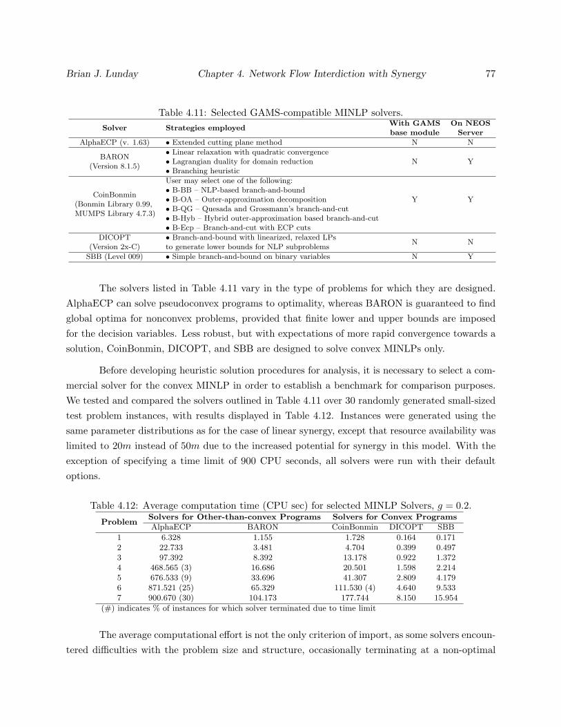
Brian J. Lunday Chapter 4. Network Flow Interdiction with Synergy 77
Table 4.11: Selected GAMS-compatible MINLP solvers.Solver Strategies employed
With GAMS On NEOSbase module Server
AlphaECP (v. 1.63) • Extended cutting plane method N N
BARON• Linear relaxation with quadratic convergence
N Y(Version 8.1.5)
• Lagrangian duality for domain reduction• Branching heuristic
User may select one of the following:
Y YCoinBonmin
• B-BB – NLP-based branch-and-bound
(Bonmin Library 0.99,• B-OA – Outer-approximation decomposition
MUMPS Library 4.7.3)• B-QG – Quesada and Grossmann’s branch-and-cut• B-Hyb – Hybrid outer-approximation based branch-and-cut• B-Ecp – Branch-and-cut with ECP cuts
DICOPT • Branch-and-bound with linearized, relaxed LPsN N
(Version 2x-C) to generate lower bounds for NLP subproblems
SBB (Level 009) • Simple branch-and-bound on binary variables N Y
The solvers listed in Table 4.11 vary in the type of problems for which they are designed.AlphaECP can solve pseudoconvex programs to optimality, whereas BARON is guaranteed to findglobal optima for nonconvex problems, provided that finite lower and upper bounds are imposedfor the decision variables. Less robust, but with expectations of more rapid convergence towards asolution, CoinBonmin, DICOPT, and SBB are designed to solve convex MINLPs only.
Before developing heuristic solution procedures for analysis, it is necessary to select a com-mercial solver for the convex MINLP in order to establish a benchmark for comparison purposes.We tested and compared the solvers outlined in Table 4.11 over 30 randomly generated small-sizedtest problem instances, with results displayed in Table 4.12. Instances were generated using thesame parameter distributions as for the case of linear synergy, except that resource availability waslimited to 20m instead of 50m due to the increased potential for synergy in this model. With theexception of specifying a time limit of 900 CPU seconds, all solvers were run with their defaultoptions.
Table 4.12: Average computation time (CPU sec) for selected MINLP Solvers, g = 0.2.
ProblemSolvers for Other-than-convex Programs Solvers for Convex ProgramsAlphaECP BARON CoinBonmin DICOPT SBB
1 6.328 1.155 1.728 0.164 0.1712 22.733 3.481 4.704 0.399 0.4973 97.392 8.392 13.178 0.922 1.3724 468.565 (3) 16.686 20.501 1.598 2.2145 676.533 (9) 33.696 41.307 2.809 4.1796 871.521 (25) 65.329 111.530 (4) 4.640 9.5337 900.670 (30) 104.173 177.744 8.150 15.954
(#) indicates % of instances for which solver terminated due to time limit
The average computational effort is not the only criterion of import, as some solvers encoun-tered difficulties with the problem size and structure, occasionally terminating at a non-optimal

Brian J. Lunday Chapter 4. Network Flow Interdiction with Synergy 78
value. In a few cases, solvers erred by eliminating all rows and columns during over-aggressivepreprocessing, while others encountered scaling difficulties for NLP subproblems with optima nearor at zero. During testing, the solver-reported optima were compared to determine relative devia-tions from the best reported solution for each instance in order to identify which solvers were likelyto encounter more difficulty when solving medium- and larger-sized problems. Table 4.13 displaysthe number of instances for which each solver failed to obtain an optimal value within the relativetolerances indicated.
Table 4.13: Number of solver failures for (1 / 0.1 / 0.01 / 0.001 / 0.0001)% relative tolerances over30 instances of each problem, g = 0.2.
Problem
Solver for Solver forSolvers for Convex ProgramsPseudoconvex Nonconvex
Programs ProgramsAlphaECP BARON CoinBonmin DICOPT SBB
1 0/0/0/0/0 0/1/1/1/1 0/0/0/0/0 1/1/1/1/1 0/0/0/0/02 0/0/0/1/1 0/1/1/1/1 0/1/1/1/1 0/1/2/2/2 0/0/0/0/03 0/0/0/0/0 1/3/3/3/3 3/7/7/7/7 1/2/2/2/2 0/0/0/0/04 0/0/0/2/3 0/0/0/0/1 4/5/5/5/5 0/1/1/1/1 0/0/0/0/05 0/0/0/1/1 0/0/1/1/2 5/6/7/7/7 0/1/1/1/1 0/0/0/0/06 3/3/3/3/3 0/1/1/1/1 18/19/19/19/19 3/3/3/3/3 0/0/0/0/07 13/15/15/16/16 0/2/2/2/2 14/17/17/17/17 4/6/6/6/6 0/0/0/0/0
Although DICOPT consumed the least average computational time, we select SBB as thecommercial solver for the baseline algorithm for comparison purposes on this convex program dueto its combination of speed and precision. Of note, the BARON solver did perform best withrespect to solver failure-rate when its default NLP solver of MINOS was permitted. However, onproblems larger than (10 × 10), when using MINOS instead of CONOPT as an NLP subproblemsolver, both BARON and SBB resulted in failure rates exceeding 90%, whereas applying heuristicsto solve MIPs on tightened feasible regions produced better objective values.
Accordingly, we test and compare the following procedures with respect to solution qualityand computational effort:
1. Commercial Software SBB: We apply SBB, a commercial, GAMS-compatible MINLP solverwith a time limit of 1800 CPU seconds per instance. The solver calls CPLEX (Version 11.1)for solving MIP master problems and CONOPT for solving NLP subproblems. The absoluteoptimality tolerance for the solver is 0, but the relative optimality tolerance was set to 10−4
(0.01%).
2. Heuristic #1 – Inner-linearization: We employ a piecewise linear approximation to thenonlinear constraints and employ ILOG CPLEX to solve the resulting MIP. Upon termina-tion, we fix the pijk-variables at the resulting optimal values; next utilize the constraints ofProblem NL1 to determine the corresponding maximal σij-variable values according to σij =
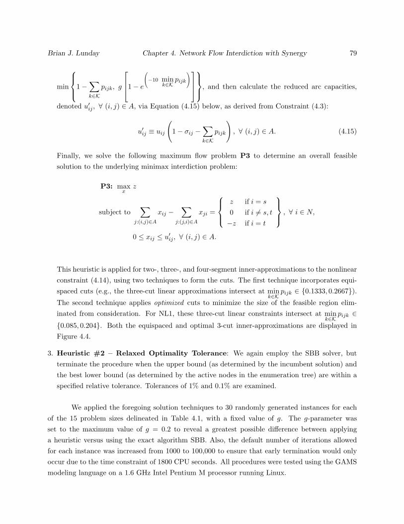
Brian J. Lunday Chapter 4. Network Flow Interdiction with Synergy 79
min
1−∑k∈K
pijk, g
1− e
(−10 min
k∈Kpijk
), and then calculate the reduced arc capacities,
denoted u′ij , ∀ (i, j) ∈ A, via Equation (4.15) below, as derived from Constraint (4.3):
u′ij ≡ uij
(1− σij −
∑k∈K
pijk
), ∀ (i, j) ∈ A. (4.15)
Finally, we solve the following maximum flow problem P3 to determine an overall feasiblesolution to the underlying minimax interdiction problem:
P3: maxx
z
subject to∑
j:(i,j)∈A
xij −∑
j:(j,i)∈A
xji =
z if i = s
0 if i 6= s, t
−z if i = t
, ∀ i ∈ N,
0 ≤ xij ≤ u′ij , ∀ (i, j) ∈ A.
This heuristic is applied for two-, three-, and four-segment inner-approximations to the nonlinearconstraint (4.14), using two techniques to form the cuts. The first technique incorporates equi-spaced cuts (e.g., the three-cut linear approximations intersect at min
k∈Kpijk ∈ 0.1333, 0.2667).
The second technique applies optimized cuts to minimize the size of the feasible region elim-inated from consideration. For NL1, these three-cut linear constraints intersect at min
k∈Kpijk ∈
0.085, 0.204. Both the equispaced and optimal 3-cut inner-approximations are displayed inFigure 4.4.
3. Heuristic #2 – Relaxed Optimality Tolerance: We again employ the SBB solver, butterminate the procedure when the upper bound (as determined by the incumbent solution) andthe best lower bound (as determined by the active nodes in the enumeration tree) are within aspecified relative tolerance. Tolerances of 1% and 0.1% are examined.
We applied the foregoing solution techniques to 30 randomly generated instances for eachof the 15 problem sizes delineated in Table 4.1, with a fixed value of g. The g-parameter wasset to the maximum value of g = 0.2 to reveal a greatest possible difference between applyinga heuristic versus using the exact algorithm SBB. Also, the default number of iterations allowedfor each instance was increased from 1000 to 100,000 to ensure that early termination would onlyoccur due to the time constraint of 1800 CPU seconds. All procedures were tested using the GAMSmodeling language on a 1.6 GHz Intel Pentium M processor running Linux.
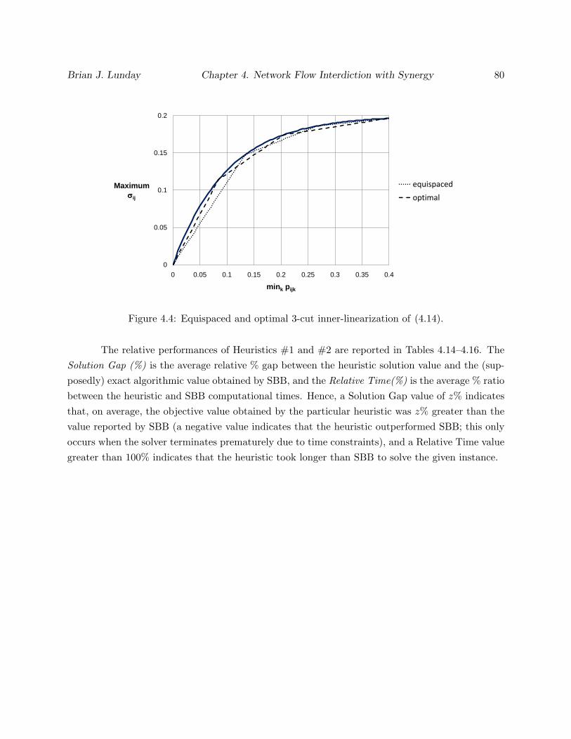
Brian J. Lunday Chapter 4. Network Flow Interdiction with Synergy 80
0
0.05
0.1
0.15
0.2
0 0.05 0.1 0.15 0.2 0.25 0.3 0.35 0.4
Maximum
ij
mink pijk
equispaced
optimal
Figure 4.4: Equispaced and optimal 3-cut inner-linearization of (4.14).
The relative performances of Heuristics #1 and #2 are reported in Tables 4.14–4.16. TheSolution Gap (%) is the average relative % gap between the heuristic solution value and the (sup-posedly) exact algorithmic value obtained by SBB, and the Relative Time(%) is the average % ratiobetween the heuristic and SBB computational times. Hence, a Solution Gap value of z% indicatesthat, on average, the objective value obtained by the particular heuristic was z% greater than thevalue reported by SBB (a negative value indicates that the heuristic outperformed SBB; this onlyoccurs when the solver terminates prematurely due to time constraints), and a Relative Time valuegreater than 100% indicates that the heuristic took longer than SBB to solve the given instance.

Brian J. Lunday Chapter 4. Network Flow Interdiction with Synergy 81
Table 4.14: Heuristic #1 (equispaced cuts) average performance vs. GAMS/SBB, g = 0.2.
Problem2-Cuts 3-Cuts 4-Cuts
Soln Gap(%) Rel Time(%) Soln Gap(%) Rel Time(%) Soln Gap(%) Rel Time(%)
1 2.375 19.263 1.718 26.337 1.330 29.0302 1.920 17.649 1.516 22.115 1.188 26.8813 2.399 7.310 2.307 8.725 2.269 11.2984 2.345 10.671 2.298 13.464 2.116 16.7925 1.897 6.128 1.626 8.546 1.558 11.2536 1.768 5.783 1.940 8.140 1.431 10.2267 2.400 4.970 2.253 6.784 1.727 8.964
Average (1–7) 2.158 10.253 1.951 13.444 1.660 16.349
8 2.123 6.081 1.921 8.246 1.963 10.5409 2.333 3.265 2.419 4.577 1.943 5.94710 2.177 3.590 2.338 4.905 2.472 6.32511 1.627 3.758 1.606 5.232 1.778 6.684
Average (8–11) 2.065 4.174 2.071 5.740 2.039 7.374
12 2.735 2.625 2.919 3.630 2.801 4.69613 -0.909 3.330 -0.374 4.431 -0.363 5.82014 -37.417 12.677 -37.241 16.444 -37.009 20.72815 -78.760 34.817 -78.552 46.527 -78.767 57.531
Average (12–15) -28.588 13.363 -28.312 17.758 -28.334 22.194
Overall Average -6.066 9.461 -6.087 12.540 -6.237 15.514
Table 4.15: Heuristic #1 (optimized cuts) average performance vs. GAMS/SBB, g = 0.2.
Problem2-Cuts 3-Cuts 4-Cuts
Soln Gap(%) Rel Time(%) Soln Gap(%) Rel Time(%) Soln Gap(%) Rel Time(%)
1 1.903 22.237 1.434 27.553 1.284 30.7062 1.629 19.032 1.179 23.195 1.471 29.4583 2.483 8.036 2.424 10.676 2.057 12.8904 2.389 10.711 2.101 14.259 2.185 18.7285 1.627 7.219 1.462 9.559 1.394 13.0336 2.040 6.403 1.458 9.207 1.607 12.6757 2.365 5.291 1.751 7.834 1.887 10.643
Average (1–7) 2.062 11.275 1.687 14.612 1.698 18.305
8 2.140 6.694 1.771 9.218 1.898 12.1879 2.366 3.641 2.190 5.371 2.667 7.42210 2.157 3.992 2.963 5.521 2.893 7.32811 1.702 4.142 1.804 6.021 1.815 7.976
Average (8–11) 2.091 4.617 2.182 6.533 2.318 8.728
12 3.063 2.936 2.416 4.196 2.248 5.67113 -0.646 3.717 -0.221 5.338 -0.376 7.26114 -37.251 14.261 -37.123 19.088 -37.215 25.21015 -78.514 40.060 -78.774 54.889 -78.771 70.410
Average (12–15) -28.337 15.244 -28.425 20.878 -28.529 27.138
Overall Average -6.036 10.558 -6.211 14.128 -6.197 18.106

Brian J. Lunday Chapter 4. Network Flow Interdiction with Synergy 82
Table 4.16: Heuristic #2 average performance vs. GAMS/SBB, g = 0.2.
Problem1% Optimality Tolerance 0.1% Optimality ToleranceSoln Gap(%) Rel Time(%) Soln Gap(%) Rel Time(%)
1 0.000 57.035 0.000 61.6962 0.010 55.389 0.000 63.9703 0.048 59.069 0.000 71.4644 0.000 55.296 0.000 57.6465 0.001 51.135 0.001 61.0456 0.000 57.114 0.000 66.2557 0.063 61.326 0.000 69.660
Average (1–7) 0.018 56.623 0.000 64.534
8 0.002 60.820 0.000 69.1349 0.046 60.403 0.003 70.31310 0.010 56.826 0.003 68.53411 0.042 53.210 0.000 68.214
Average (8–11) 0.025 57.815 0.002 69.049
12 0.046 66.358 0.005 73.49513 -2.285 87.707 -2.001 97.00614 -38.321 96.399 -38.525 105.87015 -77.960 98.627 -78.971 97.237
Average (12–15) -29.630 87.273 -29.873 93.402
Overall Average -7.886 65.114 -7.966 73.436
The SBB solver encountered difficulties for the large-sized problems, as evidenced by thenegative average Solution Gap values for instances of Problems 13–15 in Tables 4.14–4.16. Prema-ture terminations of SBB occurred primarily due to the computational time limit, excepting oneinstance for which the intermediate solver (CONOPT3) failed. The early termination frequenciesfor SBB were 93.33%, 96.67%, and 100% for the instances of Problems 13, 14, and 15, respectively.Regarding the final objective function values reported, Heuristic #1 outperformed SBB on 26.67%,100%, and 100% of the instances for Problems 13, 14, and 15, respectively.
For small and medium-sized problems, as expected, Heuristic #2 with a 0.1% toleranceoutperformed all variants of Heuristic #1 with a modest savings in computational time. However,Heuristic #2 also encountered early termination due to time constraints on instances of Problems13–15, with aggregate average failure rates of 82.22% and 95.56% for the 1% and 0.1% relativetolerance implementations, respectively. Similar to the exact algorithm, it is expected that, as thenetwork size increases beyond that of Problem 15, the early termination of Heuristic #2 will resultin solutions that are inferior to those derived by Heuristic #1.
It is also relevant to note from Tables 4.14 and 4.15 that the use of optimized cuts wasnot consistently better than using equispaced cuts, with differences being marginal, although it didrequire 17.03% more computational effort over the range of problems examined.
Due to the poor performance of SBB on the larger-sized problems, we conducted a furthercomparison of the Node 0 solution from the solver BARON with the solution produced by Heuristic

Brian J. Lunday Chapter 4. Network Flow Interdiction with Synergy 83
#1. The relative performance of the BARON software, terminated upon attaining a Node 0 solutionor consuming 1800 CPU seconds, whichever occurs first, was superior to Heuristic #1 for small-and medium-sized problems, attaining solutions with an average relative optimality gap of 0.008%for Problems 1–7, and 0.912% for Problems 8–11, based on the exact solutions as determined by theSBB software, albeit at average relative times of 1864.1% and 1566.4%, respectively. (The averagerelative times for BARON compared with SBB for Problems 8–11 would have been greater withan increased time limit, since BARON terminated prematurely at Node 0 for 50% and 100% of theinstances for Problems 9 and 10–11, respectively.) However, BARON was unable to obtain even afeasible solution for instances of the large-sized Problems 12–15.
The most robust procedure over all problem sizes turns out to be Heuristic #1 with fourequispaced cuts. Heuristic #1 achieved solution values within 3% of optimality at an averageacross all problem sizes for which SBB obtained an optimum within 1800 CPU seconds, whilesaving 85.94% of computational effort, and with a uniformly advantageous performance for larger-sized problems. Overall, this variant of Heuristic #1 improved the quality of solutions found bySBB by 6.2%, in about 15.5% of the required computational effort.
4.3.2 Nonlinear Synergy with a Convex-concave Synergy Function
In this section, we consider a convex-concave limiting function for synergy as given by
σij ≤g′ e30pijk
2000 + 5e30pijk, ∀ (i, j) ∈ A, k ∈ K, with 0 ≤ g′ ≤ 1, (4.16)
which is depicted in Figure 4.5.
The motivation for this synergy function is that, at lower levels of resource commitment(convex portion), the benefits due to synergy might become increasingly evident as additionalunits of resources are committed, whereas at higher resource levels, as min
k∈Kpijk increases (concave
portion), we might expect diminishing marginal returns of synergy to set in as before. Note thatin Equation (4.16), the parameters have been adjusted so that the point of inflection occurs atmink∈K
pijk = 0.2, and that we again have σij ≤ 0.2, ∀ (i, j) ∈ A. However, to ensure that σij = 0
whenever pijk = 0 for any k ∈ K (Constraint (4.16) yields σij = 0.0004 in this case), we incorporatean additional linear constraint, σij ≤ f pijk, ∀ (i, j) ∈ A, k ∈ K, where f = 0.662 is suitablyselected so that (4.16) implies this linear relationship for pijk ≤ 0.001. Applying this limitingfunctional form for synergy within Problem P2 as before, the resulting nonconvex MINLP is stated

Brian J. Lunday Chapter 4. Network Flow Interdiction with Synergy 84
0
0.05
0.1
0.15
0.2
0 0.05 0.1 0.15 0.2 0.25 0.3 0.35 0.4
Maximum
ij
mink pijk
Figure 4.5: Constraint (4.16) for nonlinear synergy with g′ = 1.
as Problem NL2 below:
NL2: minp,σ,α,π
∑(i,j)∈A
uijπijk
subject to αi − αj + πijk +∑k∈K
pijk + σij ≥ 0, ∀ (i, j) ∈ A,∑(i,j)∈A
cijk pijk ≤ Rk, ∀ k ∈ K,∑k∈K
pijk + σij ≤ 1, ∀ (i, j) ∈ A, (4.17)
σij ≤g′ e30pijk
2000 + 5e30pijk, ∀ (i, j) ∈ A, k ∈ K, (4.18)
σij ≤ 0.662 pijk, ∀ (i, j) ∈ A, k ∈ K, (4.19)
(σij , πij) ≥ 0, ∀ (i, j) ∈ A,
αi ∈ 0, 1 , ∀ i ∈ N, with αs = 0 and αt = 1.
Since NL2 is not a convex program, most commercial solvers do not guarantee the abilityto obtain a globally optimal solution. BARON is a notable exception, and was selected to serve asa benchmark in this study (with a time limit of 1800 CPU seconds). Several heuristic approacheswere investigated as described below, all of which were modeled within GAMS and solved invokingcombinations of commercial solvers:

Brian J. Lunday Chapter 4. Network Flow Interdiction with Synergy 85
1. Commercial software BARON: We employed GAMS/BARON as an exact optimizer, usingCPLEX to solve the LP subproblems, and SNOPT to solve the NLP subproblems. As before,the relative optimality tolerance was set at 10−4.
2. Heuristic H1: This employs GAMS/BARON, but terminates the algorithm after Node 0.
3. Heuristic H2: As in the previous section, this employs the commercial software SBB (whichis, however, designed for convex programs).
4. Heuristic H3 – Inner-linearization: This is akin to Heuristic #1 for NL1, with two excep-tions. In the first step, an inner-linearization is accomplished by replacing Constraints (4.18)–(4.19) with σij ≤ 0.0405 pijk, ∀ (i, j) ∈ A, k ∈ K, which passes through the origin in Figure 4.5and is tangential to Constraint (4.18) at a point lying on the convex part of the function given bythe right-hand side of (4.18), i.e., at the point (0.0335, 0.001357), so that this yields a restrictionof Problem NL2 (see Figure 4.6). The resulting pijk-values are fixed. In the second step, thecorresponding maximal σij-variable values are computed subject to Constraints (4.17)–(4.19),before updating the arc capacities via Equation (4.15) and solving Problem P3 to determine anoverall final feasible solution to the underlying minimax interdiction problem.
0
0.05
0.1
0.15
0.2
0 0.05 0.1 0.15 0.2 0.25 0.3 0.35 0.4
Maximum
ij
mink pijk
H3
H4
H5
Figure 4.6: Heuristics H3, H4, and H5 with m = 3 applied to Constraint (4.16), with g′ = 1.
5. Heuristic H4 – Piecewise linear approximation: In this procedure, as depicted in Figure4.6, we construct an m-segment piecewise approximation to Constraint (4.18) using equidistantbreakpoints, and solve the resulting mixed-integer program using CPLEX. We next fix the pijk-variables at the derived optimal values, and then proceed as in Heuristic H3 to determine the final

Brian J. Lunday Chapter 4. Network Flow Interdiction with Synergy 86
solution. For this technique, we tested m ∈ 2, 3, 4 for the piecewise approximation granularity;the corresponding variants are henceforth referred to as H4-2, H4-3, and H4-4. Note that thismethod becomes asymptotically exact as the granularity of the piecewise linear approximationincreases.
6. Heuristic H5 – Outer-approximation: This procedure adopts an outer-approximation of
the synergy function, composed of the chord that passes through(
mink∈K
pijk, σij
)= (0, 0) and is
tangential to Constraint (4.18) (where the point of tangency occurs at (0.2642, 0.1748)), alongwith an m-segment tangential outer-approximation over the remaining concave portion of thesynergy function, including a final one at min
k∈Kpijk = 0.4 (See Figure 4.6). For implementation,
we utilized m ∈ 2, 3, 4, where the corresponding variants are referred to as H5-2, H5-3, and H5-4, respectively. Again, we solve the resulting linearized problem, fix the resulting pijk-variablevalues, and proceed as in Heuristic H3 to determine the final solution.
We applied the exact algorithm BARON and the foregoing nine heuristic variants to solve30 randomly generated instances for each of the 15 test problem sizes delineated in Table 4.1,setting g′ = 1 to maximize the potential benefits of synergy in the formulation, thereby magnifyingthe discrepancies in the heuristic approximations. Heuristics H2–H5 were employed with a relativeoptimality tolerance of 10−4, identical to that used for BARON. The maximum number of iterationsfor each solution technique was limited to 100,000 with a time constraint of 1800 CPU seconds.All procedures were tested using the GAMS modeling language on a 1.6 GHz Intel Pentium Mprocessor running Linux. During testing, BARON did not always produce the best reported valuefor each instance. Therefore, the Solution Gap for each technique was measured against the bestreported value across all methods for each instance; Table 4.17 displays the average values of theSolution Gap thus obtained.
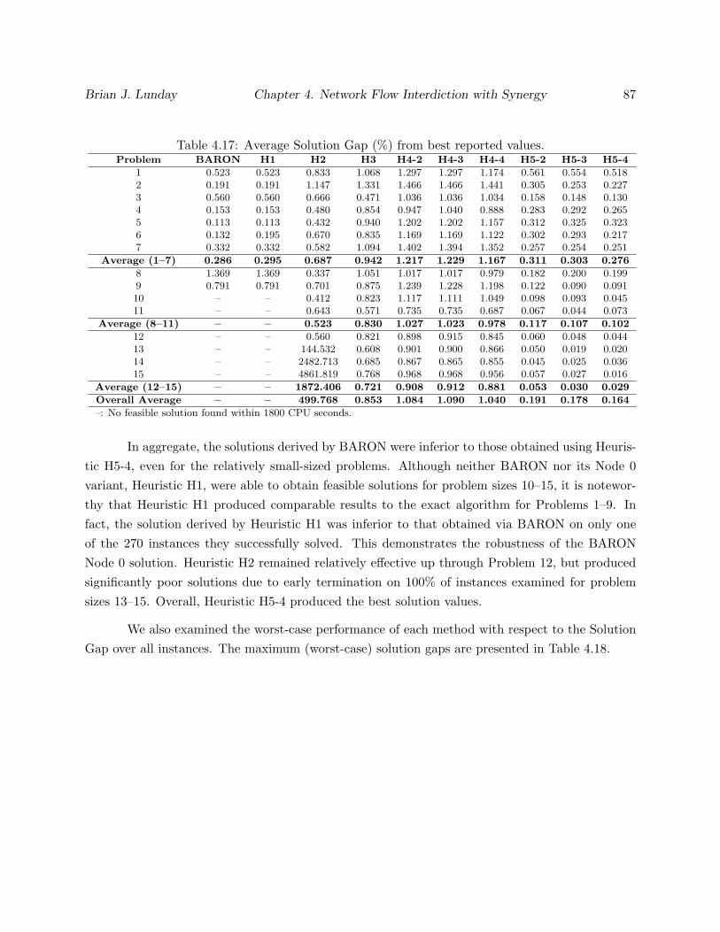
Brian J. Lunday Chapter 4. Network Flow Interdiction with Synergy 87
Table 4.17: Average Solution Gap (%) from best reported values.Problem BARON H1 H2 H3 H4-2 H4-3 H4-4 H5-2 H5-3 H5-4
1 0.523 0.523 0.833 1.068 1.297 1.297 1.174 0.561 0.554 0.5182 0.191 0.191 1.147 1.331 1.466 1.466 1.441 0.305 0.253 0.2273 0.560 0.560 0.666 0.471 1.036 1.036 1.034 0.158 0.148 0.1304 0.153 0.153 0.480 0.854 0.947 1.040 0.888 0.283 0.292 0.2655 0.113 0.113 0.432 0.940 1.202 1.202 1.157 0.312 0.325 0.3236 0.132 0.195 0.670 0.835 1.169 1.169 1.122 0.302 0.293 0.2177 0.332 0.332 0.582 1.094 1.402 1.394 1.352 0.257 0.254 0.251
Average (1–7) 0.286 0.295 0.687 0.942 1.217 1.229 1.167 0.311 0.303 0.276
8 1.369 1.369 0.337 1.051 1.017 1.017 0.979 0.182 0.200 0.1999 0.791 0.791 0.701 0.875 1.239 1.228 1.198 0.122 0.090 0.09110 – – 0.412 0.823 1.117 1.111 1.049 0.098 0.093 0.04511 – – 0.643 0.571 0.735 0.735 0.687 0.067 0.044 0.073
Average (8–11) – – 0.523 0.830 1.027 1.023 0.978 0.117 0.107 0.102
12 – – 0.560 0.821 0.898 0.915 0.845 0.060 0.048 0.04413 – – 144.532 0.608 0.901 0.900 0.866 0.050 0.019 0.02014 – – 2482.713 0.685 0.867 0.865 0.855 0.045 0.025 0.03615 – – 4861.819 0.768 0.968 0.968 0.956 0.057 0.027 0.016
Average (12–15) – – 1872.406 0.721 0.908 0.912 0.881 0.053 0.030 0.029
Overall Average – – 499.768 0.853 1.084 1.090 1.040 0.191 0.178 0.164
–: No feasible solution found within 1800 CPU seconds.
In aggregate, the solutions derived by BARON were inferior to those obtained using Heuris-tic H5-4, even for the relatively small-sized problems. Although neither BARON nor its Node 0variant, Heuristic H1, were able to obtain feasible solutions for problem sizes 10–15, it is notewor-thy that Heuristic H1 produced comparable results to the exact algorithm for Problems 1–9. Infact, the solution derived by Heuristic H1 was inferior to that obtained via BARON on only oneof the 270 instances they successfully solved. This demonstrates the robustness of the BARONNode 0 solution. Heuristic H2 remained relatively effective up through Problem 12, but producedsignificantly poor solutions due to early termination on 100% of instances examined for problemsizes 13–15. Overall, Heuristic H5-4 produced the best solution values.
We also examined the worst-case performance of each method with respect to the SolutionGap over all instances. The maximum (worst-case) solution gaps are presented in Table 4.18.

Brian J. Lunday Chapter 4. Network Flow Interdiction with Synergy 88
Table 4.18: Worst-case Solution Gap (%) (from best reported values) over 30 instances.Problem BARON H1 H2 H3 H4-2 H4-3 H4-4 H5-2 H5-3 H5-4
1 3.380 3.380 10.679 3.400 5.199 5.199 5.199 2.539 2.539 2.5392 2.243 2.243 5.711 4.923 4.436 4.436 4.354 1.073 1.043 1.0263 3.871 3.871 3.517 2.200 4.203 4.203 4.192 1.018 0.993 1.0744 1.975 1.975 2.496 2.311 2.708 4.596 2.708 1.334 1.210 1.1975 1.423 1.423 3.793 2.850 6.514 6.514 6.514 2.683 1.942 2.7456 1.708 1.922 2.067 3.136 4.529 4.529 4.529 1.657 1.672 1.6757 2.478 2.478 5.048 4.121 5.364 5.364 5.364 1.052 1.052 1.052
Average (1–7) 2.440 2.470 4.759 3.277 4.708 4.977 4.694 1.622 1.493 1.615
8 8.396 8.396 1.632 4.053 4.678 4.678 4.678 0.740 0.922 1.2129 3.827 3.827 2.037 2.725 3.362 3.362 3.267 0.554 0.441 0.46010 – – 1.521 3.937 3.313 3.313 3.313 0.599 0.452 0.39111 – – 2.352 1.655 1.896 1.896 1.896 0.306 0.315 0.320
Average (8–11) – – 1.885 3.093 3.312 3.312 3.289 0.550 0.532 0.596
12 – – 2.518 2.432 3.336 3.572 3.160 0.518 0.218 0.25413 – – 2271.884 1.903 2.578 2.578 2.578 0.188 0.200 0.12714 – – 9026.113 2.619 2.943 2.943 2.922 0.258 0.181 0.23115 – – 10222.434 2.482 3.214 3.214 3.214 0.397 0.212 0.153
Average (12–15) – – 5380.737 2.359 3.018 3.077 2.969 0.341 0.203 0.191
Overall Average – – 1437.587 2.983 3.885 4.027 3.859 0.994 0.893 0.964
–: No feasible solution found within 1800 CPU seconds.
The worst-case performance of Heuristic H5 is superior to other techniques in aggregateas well as over almost all problem sizes, with three tangential supports (H5-3) producing the bestresults. This observation holds even when the comparison is restricted to problem sizes that aresolved by BARON or SBB (H2).
Also, note the inferior worst-case performances of Heuristics H2, H3, and H4. For SBB(H2), the significant deviation from the best reported values results from the nonconvexity of theproblem, because the solver terminates upon finding a local optimum. Whereas the worst-case per-formance for the outer-approximation heuristics H5-2, H5-3, and H5-4 were within 3% of the bestreported values over all instances examined, the worst-case performance for the piecewise linearapproximation heuristics H4-2, H4-3, and H4-4, and the inner-approximation heuristic (H3) wererespectively within 7% and 5% of the best reported values over all instances. The inferior perfor-mance of Heuristic H3 reflects the predominance of higher levels of synergy in optimal solutions forsome of the instances examined, wherein the inner-approximation does not consider the relevantportion of the feasible region in its first phase of implementation. (In a sequel discussed laterin this section, we also modified Heuristic H4 by utilizing one linearization segment as the chordover the convex region of Constraint (4.16), and augmenting this with m additional segments withequidistant spacing between breakpoints to approximate the remaining concave region. Althoughthis technique improved upon the values reported by Heuristic H4, it did not rival those of HeuristicH5.)
The average and worst-case performances reported in Tables 4.17 and 4.18 present an in-

Brian J. Lunday Chapter 4. Network Flow Interdiction with Synergy 89
complete representation of the heuristics’ potential, from which an observer might prematurelyinfer that H4 should be discarded as a viable approach. Table 4.19 reports the number of instances(out of 30) for which each solution technique’s reported optimal objective function value was equalto the best reported value. As before, no values are reported for the full implementation of BARONor H1 on Problems 10–15, for which neither technique obtained feasible solutions within 1800 CPUseconds on any of the instances examined.
Table 4.19: Number of Instances each Heuristic Obtained a Best Reported Value.Problem BARON H1 H2 H3 H4-2 H4-3 H4-4 H5-2 H5-3 H5-4
1 9 9 7 0 8 8 10 2 3 52 11 11 1 0 4 4 7 0 4 73 7 7 2 4 8 8 8 8 5 94 8 7 5 0 5 5 7 2 6 85 8 8 1 1 8 8 8 3 3 106 7 7 3 1 6 6 7 2 2 107 6 6 4 1 4 4 4 4 4 10
Average (1–7) 8 7.857 3.286 1 6.143 6.143 7.286 3 3.857 8.429
8 2 2 5 0 3 3 6 4 4 99 5 5 3 0 1 1 1 4 6 1310 – – 4 1 2 2 3 3 3 1611 – – 1 1 5 5 7 5 7 9
Average (8–11) – – 3.25 0.5 2.75 2.75 4.25 4 5 11.75
12 – – 2 0 2 2 2 8 7 1113 – – 0 0 0 1 1 1 10 1714 – – 0 1 1 1 1 8 8 1215 – – 0 0 0 0 0 3 5 22
Average (12–15) – – 0.5 0.25 0.75 1 1 5 7.5 15.5
Overall Average – – 3.444 0.778 5.222 5.222 6.444 3.222 4.111 9
–: No feasible solution found within 1800 CPU seconds.
Based on this measure of best-case performances, H4 variants are highly competitive onsmall-sized problems, and the relative dominance of H5 variants, and more specifically H5-4, onlybecomes apparent on mid- and large-sized problems. As a further consideration, we modify H4 todevelop heuristic variants that are more directly comparable in construction to H5. Genericallydenoted Heuristic H4+, this technique constructs for variant H4+-m an (m+1)-segment piece-wise approximation to Constraint (4.18), wherein the first segment occurs between the breakpoints(0, 0) and (0.2642, 0.1748), identical to the chord constructed over the convex region of the syn-ergy function for Heuristic H5-m. The breakpoints for the remaining m segments of H4+-m areequidistantly spaced over the concave region of the synergy function. Hence, this approximationand the relaxation used in H5-m respectively employ an inner- and outer-approximation over theconcave region of the synergy curve. In addition to the representation of H4+-m as a mixed-integerprogram using Type 2 Special Ordered Sets, we also examine an alternative formulation H4(L)+
(with variants H4(L)+-m) in which we convert each (concave) piecewise approximation to Con-straint (4.18) in H4+-m to (m+1) linear bounding constraints. We tested Heuristics H4+, H4(L)+,and H5 for m ∈ 2, 3, 4 on the same battery of problems, instances, and termination criteria asin Tables 4.17–4.21. Table 4.20 reports the average values of the relative solution gap (%) for each

Brian J. Lunday Chapter 4. Network Flow Interdiction with Synergy 90
heuristic variant from the best value obtained using the nine tested procedures.
Table 4.20: Average Solution Gap (%) for H4+, H4(L)+, and H5 from best reported values.Problem H4+-2 H4+-3 H4+-4 H4(L)+-2 H4(L)+-3 H4(L)+-4 H5-2 H5-3 H5-4
1 0.944 0.916 0.903 0.755 0.617 0.483 0.208 0.201 0.1662 1.307 1.305 1.305 1.029 0.919 0.936 0.148 0.095 0.0693 0.944 0.942 0.942 0.575 0.449 0.469 0.066 0.056 0.0384 0.706 0.705 0.694 0.467 0.343 0.331 0.054 0.063 0.0365 1.037 1.000 1.000 0.812 0.731 0.695 0.129 0.142 0.1396 1.092 1.083 1.065 0.659 0.707 0.692 0.229 0.220 0.1457 1.237 1.216 1.205 0.774 0.726 0.709 0.090 0.087 0.084
Average (1–7) 1.038 1.024 1.016 0.724 0.642 0.616 0.132 0.123 0.097
8 0.937 0.951 0.940 0.691 0.602 0.589 0.102 0.120 0.1199 1.180 1.162 1.162 0.706 0.604 0.514 0.073 0.041 0.04310 1.095 1.075 1.039 0.660 0.667 0.594 0.072 0.067 0.02011 0.725 0.722 0.705 0.556 0.538 0.388 0.057 0.034 0.063
Average (8–11) 0.984 0.978 0.961 0.653 0.603 0.522 0.076 0.066 0.061
12 0.884 0.879 0.862 0.742 0.623 0.573 0.049 0.038 0.03313 1.199 1.196 1.173 0.825 0.692 0.600 0.051 0.051 0.02214 0.868 0.865 0.855 0.711 0.654 0.577 0.043 0.023 0.03415 0.970 0.965 0.962 0.672 0.569 0.533 0.057 0.027 0.016
Average (12–15) 0.980 0.976 0.963 0.737 0.634 0.571 0.050 0.035 0.026
Overall Average 1.008 0.999 0.987 0.709 0.629 0.579 0.095 0.084 0.068
The difference in the performance of H4+-m compared to H4(L)+-m for any given m-parameter is directly attributable to the inherent difficulties for the solver to optimize the H4+-mformulation, which requires (m+1)|A| additional binary decision variables compared to H4(L)+-mfor constructing the piecewise linear approximations for Constraint (4.18). Of course, the formu-lations H4(L)+-m and H5-m are asymptotically equivalent as m approaches infinity, but for thelower values of m we consider, Heuristic H5 with four tangential supports remains as the prescribedtechnique to solve Problem NL2.
Table 4.21 presents the Relative Time (%) performance results for all the procedures, usingBARON as the benchmark for comparison. The effort for Heuristic H1 was comparable to thatfor the full implementation of BARON, but all other heuristics yielded a significant improvement.While the local search procedure in Heuristic H2 (SBB solver) achieved significant time savings(97.59% on average), the remaining MIP-based heuristics resulted in a 2-3 orders of magnitudeimprovement in computational time. Although Heuristic H5-4 required somewhat less average com-putational time than H5-3 (both consuming roughly only 0.67% of the effort required by BARONon average), this result no longer holds if the outlying poor performance of H5-3 on Problem 1is omitted from consideration. Nonetheless, Heuristic H5-4 yields the best compromise betweensolution quality and computational effort.
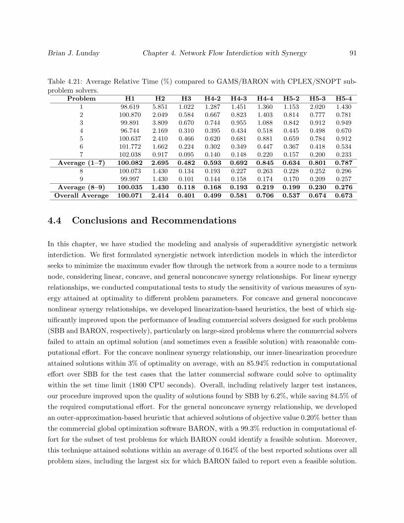
Brian J. Lunday Chapter 4. Network Flow Interdiction with Synergy 91
Table 4.21: Average Relative Time (%) compared to GAMS/BARON with CPLEX/SNOPT sub-problem solvers.
Problem H1 H2 H3 H4-2 H4-3 H4-4 H5-2 H5-3 H5-4
1 98.619 5.851 1.022 1.287 1.451 1.360 1.153 2.020 1.4302 100.870 2.049 0.584 0.667 0.823 1.403 0.814 0.777 0.7813 99.891 3.809 0.670 0.744 0.955 1.088 0.842 0.912 0.9494 96.744 2.169 0.310 0.395 0.434 0.518 0.445 0.498 0.6705 100.637 2.410 0.466 0.620 0.681 0.881 0.659 0.784 0.9126 101.772 1.662 0.224 0.302 0.349 0.447 0.367 0.418 0.5347 102.038 0.917 0.095 0.140 0.148 0.220 0.157 0.200 0.233
Average (1–7) 100.082 2.695 0.482 0.593 0.692 0.845 0.634 0.801 0.787
8 100.073 1.430 0.134 0.193 0.227 0.263 0.228 0.252 0.2969 99.997 1.430 0.101 0.144 0.158 0.174 0.170 0.209 0.257
Average (8–9) 100.035 1.430 0.118 0.168 0.193 0.219 0.199 0.230 0.276
Overall Average 100.071 2.414 0.401 0.499 0.581 0.706 0.537 0.674 0.673
4.4 Conclusions and Recommendations
In this chapter, we have studied the modeling and analysis of superadditive synergistic networkinterdiction. We first formulated synergistic network interdiction models in which the interdictorseeks to minimize the maximum evader flow through the network from a source node to a terminusnode, considering linear, concave, and general nonconcave synergy relationships. For linear synergyrelationships, we conducted computational tests to study the sensitivity of various measures of syn-ergy attained at optimality to different problem parameters. For concave and general nonconcavenonlinear synergy relationships, we developed linearization-based heuristics, the best of which sig-nificantly improved upon the performance of leading commercial solvers designed for such problems(SBB and BARON, respectively), particularly on large-sized problems where the commercial solversfailed to attain an optimal solution (and sometimes even a feasible solution) with reasonable com-putational effort. For the concave nonlinear synergy relationship, our inner-linearization procedureattained solutions within 3% of optimality on average, with an 85.94% reduction in computationaleffort over SBB for the test cases that the latter commercial software could solve to optimalitywithin the set time limit (1800 CPU seconds). Overall, including relatively larger test instances,our procedure improved upon the quality of solutions found by SBB by 6.2%, while saving 84.5% ofthe required computational effort. For the general nonconcave synergy relationship, we developedan outer-approximation-based heuristic that achieved solutions of objective value 0.20% better thanthe commercial global optimization software BARON, with a 99.3% reduction in computational ef-fort for the subset of test problems for which BARON could identify a feasible solution. Moreover,this technique attained solutions within an average of 0.164% of the best reported solutions over allproblem sizes, including the largest six for which BARON failed to report even a feasible solution.

Brian J. Lunday Chapter 4. Network Flow Interdiction with Synergy 92
For future study, we propose sociological research to better characterize and quantify thesynergy produced by group interactions. Whereas our proposed synergistic network interdictionmodels are generally applicable, they ultimately need to be calibrated with data acquired from ascientific study of group interactions and superadditive synergy relationships.

Chapter 5
Interdicting Networks to
Competitively Minimize Evasion with
Synergy Between Applied Resources
5.1 Introduction
In this chapter, we present our research on the network interdiction problems, as introduced inSection 1.1.3 and outlined in Section 1.2. We develop in Section 5.2 a model in which the resourcesare deployed overtly, resulting in a polynomial program with linear constraints. We also formulatetwo variants of this model that incorporate arc-wise superadditive synergy between resource types,where the synergy relationship is assumed to be either linear, or concave (and nonlinear) to reflectdiminishing marginal effects. In Section 5.2.3, we present models representing a second strategy inwhich resources are echeloned for overt and subsequent covert deployment, thus forgoing synergy inreturn for the opportunity to deceive the adversary. We further develop and analyze two variantsof this second model, based on whether or not the interdictor is aware of the evader’s path selectionprior to deploying the covert resources. These strategic formulations for covert resource deploy-ment are tested in Section 5.3 against overt strategies, both with and without synergy, and forcontinuous as well as integer-restricted resource allocations, to determine the comparative valuesof the corresponding resource utilization techniques. We conclude the study in Section 5.4 with asummary and recommendations for future research.
93

Brian J. Lunday Chapter 5. Competitive Probability of Evasion Problem 94
5.2 Competitive Minimization of Evasion under Overt Strategies
In this section, we examine the problem of the interdictor seeking to maximize the minimumprobability of interdicting a single unit of flow traversing a given network between a specified pairof source and terminus nodes, while employing multiple resources with synergy. We restrict theexamination to linear and concave synergy relationships similar to Problems P2 and NL1 in Sections4.2 and 4.3.1, respectively, but extend the formulation and analysis to consider two cases. In thefirst case, we assume that all the available different resources are employed overtly, achieve synergy,and the evader is aware of their use, as well as the effect on the arc interdiction probabilitiesinduced by the interdictor. In the second case, we consider the situation where some resourcesare employed overtly as above, while some other resources are deployed covertly in a mannerthat allows information sharing, but prevents the resource interactions that would induce synergywith the movitivation of limiting the evader’s situational awareness of asset allocation, potentiallycreating the opportunity for an increased net probability of interdiction.
5.2.1 Maximizing the Probability of Evasion
The baseline problem for this comparative analysis is the formulation for which an agent seeks totransport a unit of flow through a directed network while maximizing the probability of evadinginterdiction by an opponent. Let xij ∈ 0, 1 indicate whether the agent travels on arc (i, j),and let pij be the fixed probability of evading the opponent while traversing that arc. (Hence,(1− pij) is the probability of the opponent interdicting the agent on arc (i, j).) Assuming that thearc interdiction events are independent, the resulting formulation for determining an s-t path thatmaximizes the probability of evasion is as follows:
MPEP: maxx
∏(i,j)∈A
(1− xij + pijxij)
subject to∑
j:(i,j)∈A
xij −∑
j:(j,i)∈A
xji =
1 if i = s
0 if i 6= s, t
−1 if i = t
, ∀ i ∈ N,
xij ∈ 0, 1 , ∀ (i, j) ∈ A.
5.2.2 Competitive Minimization of Evasion under Overt Strategies
In order to incorporate the opponent’s actions, we now relax the assumption that the probabilitiesfor evasion, pij , are fixed. For a single interdiction resource, define rij as the amount of the

Brian J. Lunday Chapter 5. Competitive Probability of Evasion Problem 95
resource allocated to arc (i, j). As an initial case, we assume that an absence of resource allocationto an arc results in certain evasion by the agent; an allocation of cij amount of resource on arc(i, j) results in certain interdiction; and a linear relationship exists between these two extremes.(Alternative evasion probability-resource relationships are possible, and we discuss discuss therelative advantages and disadvantages of one such relationship in Section 5.3.3.) Hence, we have:
pij = 1− rijcij, where 0 ≤ rij ≤ cij , ∀ (i, j) ∈ A.
Given a fixed availability, R, for the interdictor’s resource, we consider the following formulationfrom the opponent’s viewpoint:
minr,p
maxx
∏(i,j)∈A
(1− xij + pijxij)
subject to∑
j:(i,j)∈A
xij −∑
j:(j,i)∈A
xji =
1 if i = s
0 if i 6= s, t
−1 if i = t
, ∀ i ∈ N,
∑(i,j)∈A
rij ≤ R,
pij = 1− rijcij, ∀ (i, j) ∈ A, (5.1)
xij ∈ 0, 1 , ∀ (i, j) ∈ A,
(pij , rij) ≥ 0, ∀ (i, j) ∈ A. (5.2)
Note that the restrictions pij ≤ 1, ∀ (i, j) ∈ A, and rij ≤ cij , ∀ (i, j) ∈ A, are implied by Constraints(5.1) and (5.2).
When multiple resource types are considered, indexed by k ∈ K ≡ 1, ...,K as before, weformulate the Competitive Probability of Evasion Problem (CPEP) as follows:
CPEP: minr,p
maxx
∏(i,j)∈A
(1− xij + pijxij) (5.3)
subject to∑
j:(i,j)∈A
xij −∑
j:(j,i)∈A
xji =
1 if i = s
0 if i 6= s, t
−1 if i = t
, ∀ i ∈ N, (5.4)
∑(i,j)∈A
rijk ≤ Rk, ∀ k ∈ K, (5.5)
pij = 1−∑k∈K
(rijkcijk
), ∀ (i, j) ∈ A, (5.6)
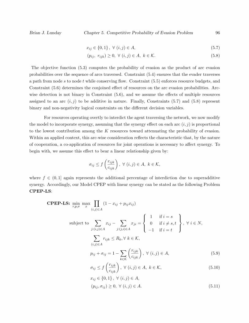
Brian J. Lunday Chapter 5. Competitive Probability of Evasion Problem 96
xij ∈ 0, 1 , ∀ (i, j) ∈ A, (5.7)
(pij , rijk) ≥ 0, ∀ (i, j) ∈ A, k ∈ K. (5.8)
The objective function (5.3) computes the probability of evasion as the product of arc evasionprobabilities over the sequence of arcs traversed. Constraint (5.4) ensures that the evader traversesa path from node s to node t while conserving flow. Constraint (5.5) enforces resource budgets, andConstraint (5.6) determines the conjoined effect of resources on the arc evasion probabilities. Arc-wise detection is not binary in Constraint (5.6), and we assume the effects of multiple resourcesassigned to an arc (i, j) to be additive in nature. Finally, Constraints (5.7) and (5.8) representbinary and non-negativity logical constraints on the different decision variables.
For resources operating overtly to interdict the agent traversing the network, we now modifythe model to incorporate synergy, assuming that the synergy effect on each arc (i, j) is proportionalto the lowest contribution among the K resources toward attenuating the probability of evasion.Within an applied context, this arc-wise consideration reflects the characteristic that, by the natureof cooperation, a co-application of resources for joint operations is necessary to affect synergy. Tobegin with, we assume this effect to bear a linear relationship given by:
σij ≤ f(rijkcijk
), ∀ (i, j) ∈ A, k ∈ K,
where f ∈ (0, 1] again represents the additional percentage of interdiction due to superadditivesynergy. Accordingly, our Model CPEP with linear synergy can be stated as the following ProblemCPEP-LS:
CPEP-LS: minr,p,σ
maxx
∏(i,j)∈A
(1− xij + pijxij)
subject to∑
j:(i,j)∈A
xij −∑
j:(j,i)∈A
xji =
1 if i = s
0 if i 6= s, t
−1 if i = t
, ∀ i ∈ N,
∑(i,j)∈A
rijk ≤ Rk,∀ k ∈ K,
pij + σij = 1−∑k∈K
(rijkcijk
), ∀ (i, j) ∈ A, (5.9)
σij ≤ f(rijkcijk
), ∀ (i, j) ∈ A, k ∈ K, (5.10)
xij ∈ 0, 1 , ∀ (i, j) ∈ A,
(pij , σij) ≥ 0, ∀ (i, j) ∈ A. (5.11)

Brian J. Lunday Chapter 5. Competitive Probability of Evasion Problem 97
Note that the non-negativity of the rijk-variables is presently induced by Constraints (5.10) and(5.11).
Alternatively, we consider a nonlinear synergy function under which the synergistic effect ofresources exhibits diminishing marginal returns for each arc (i, j). Applying a concavity structure,we restrict:
σij ≤ g
[1− e
−h
(rijkcijk
)], ∀ (i, j) ∈ A, k ∈ K, (5.12)
where g ∈ (0, 1) represents the maximum percentage of interdiction due to this form of superaddi-tive synergy (e.g., if cooperation results in at most 20% of the arc interdiction due to synergisticeffects, then g = 0.2), and h is a scaling factor to determine how rapidly the resource that leastcontributes to detection on an arc approaches the maximum synergy level. Let CPEP-NLS (non-linear synergy) denote the model obtained by incorporating the relationship (5.12) in lieu of (5.10)in the foregoing formulation, where again, rijk ≥ 0 is implied by (5.11) and (5.12).
In order to facilitate a direct solution of the CPEP models via conventional modeling andcommercial software, we adopt a path enumeration-based reformulation technique. Accordingly,define L to be the set of all simple (acyclic) paths from the source node s to the terminus t(indexed by l), and let P represent the maximum probability of an agent evading the interdictor.The resulting path enumeration formulation, CPEP(PE), for determining an optimal allocationof overt resources can be stated as follows:
CPEP(PE): minr,p
P (5.13)
subject to P ≥∏
(i,j)∈l
pij , ∀ l ∈ L, (5.14)
∑(i,j)∈A
rijk ≤ Rk, ∀ k ∈ K, (5.15)
pij = 1−∑k∈K
(rijkcijk
), ∀ (i, j) ∈ A, (5.16)
(pij , rijk) ≥ 0, ∀ (i, j) ∈ A, k ∈ K. (5.17)
In this model formulation, the set of alternative optimal evader paths is given by the active con-straints in (5.14) at optimality. Note that, whereas the explicit representation of (5.14) involvesa potentially exponential task, the nonconvex nature of this constraint inhibits the design of aneffective row generation solution algorithm. We shall therefore rely on this reformulation onlyfor manageably-sized networks, and principally for providing empirical insights into alternativestrategic policies. In a likewise fashion, we derive synergistic formulations CPEP-LS(PE) andCPEP-NLS(PE), wherein we respectively impose Equations (5.10) and (5.12), and where Equa-
Brian J. Lunday Chapter 5. Competitive Probability of Evasion Problem 98
tions (5.9) and (5.11) replace (5.16) and (5.17). For the computational study in Section 5.3, werestrict our analysis to instances having a network structure as examined in Israeli and Wood(2002), where we can enumerate the directed paths via a depth first search with backtracking anda provision to prevent cycling.
The obvious shortcoming to this approach is the cumbersome requirement to enumerate allpaths, l ∈ L. Restricting the topography for our test problems to that displayed in Figure 4.2, anm × n network will manifest |L| ≤ (3m)(n−1). Due to the exponential complexity, we will restrictour study in the following section to consider networks smaller than or equal to (m,n) = (4, 4), forwhich |L| = 1000. (A mere increase by one row and one column for the node transshipment matrixto (m,n) = (5, 5) results in |L| = 28561, for which most instances of CPEP-NLS(PE) require morethan 1800 CPU seconds to solve to global optimality with BARON.) Furthermore, the formulationis a nonconvex program due to Constraint (5.14) and, as such, CPEP(PE) and variants require arobust commercial solver to ensure global optimality. Note that this nonconvexity would remainan impediment in a relaxation approach in which the constraints (5.14) are (partially) relaxed andare iteratively generated in an as-and-when-needed fashion.
5.2.3 Competitive Evasion Models for Overt and Covert Resource Deployment
In this section, we consider the situation where some resources are employed overtly as above,while some other resources are deployed covertly in a manner that allows information sharing.However, we assume that this naturally obviates resource interactions that induce synergy, withthe motivation of limiting the evader’s situational awareness of asset allocation, and thus potentiallycreating the opportunity for an increased net probability of interdiction. Such instances occur whenthe evader’s selection of arcs to traverse after the allocation of overt resources, in accordance withrational choice theory, is limited in scope so as to allow a subsequent focused allocation of covertresources. One motivation for this problem is the employment of intelligence, surveillance, andreconnaissance (ISR) assets, such as UAVs, helicopters, or special operations forces, in supportof conventional ground-based elements. When employed in concert with ground forces (wherebysynergy is achieved), direct communication is required and the evader is more likely to be awareof their use. When employed independently (in the absence of synergy), the interdictor has less ofan overall effect on the entirety of the network, but might be more likely to interdict the evader byrestricting the latter’s movements and then applying certain additional resources covertly. Within agame-theoretic context, this compares the results of two-stage extensive form games with completeand incomplete information for the evader (see Osborne, 2004). The goal of this investigation isto determine whether optimal solution patterns favor overt action (possibly with synergy) or acombination of overt and covert strategies in the absence of synergy.
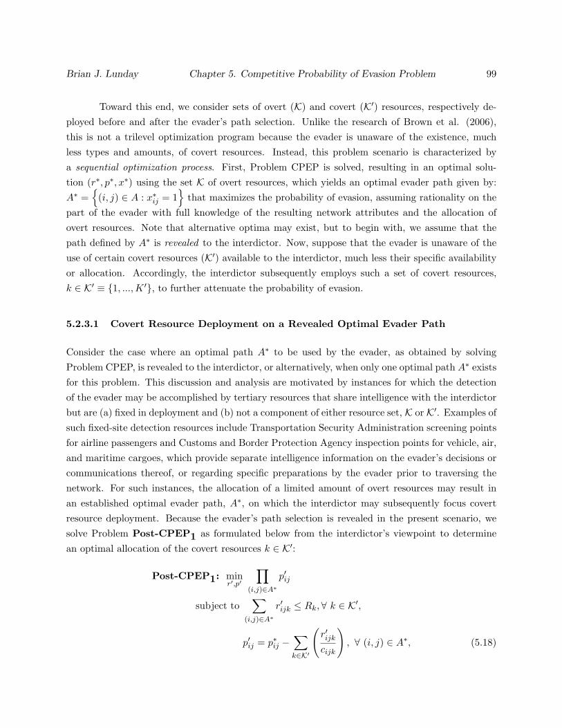
Brian J. Lunday Chapter 5. Competitive Probability of Evasion Problem 99
Toward this end, we consider sets of overt (K) and covert (K′) resources, respectively de-ployed before and after the evader’s path selection. Unlike the research of Brown et al. (2006),this is not a trilevel optimization program because the evader is unaware of the existence, muchless types and amounts, of covert resources. Instead, this problem scenario is characterized bya sequential optimization process. First, Problem CPEP is solved, resulting in an optimal solu-tion (r∗, p∗, x∗) using the set K of overt resources, which yields an optimal evader path given by:A∗ =
(i, j) ∈ A : x∗ij = 1
that maximizes the probability of evasion, assuming rationality on the
part of the evader with full knowledge of the resulting network attributes and the allocation ofovert resources. Note that alternative optima may exist, but to begin with, we assume that thepath defined by A∗ is revealed to the interdictor. Now, suppose that the evader is unaware of theuse of certain covert resources (K′) available to the interdictor, much less their specific availabilityor allocation. Accordingly, the interdictor subsequently employs such a set of covert resources,k ∈ K′ ≡ 1, ...,K ′, to further attenuate the probability of evasion.
5.2.3.1 Covert Resource Deployment on a Revealed Optimal Evader Path
Consider the case where an optimal path A∗ to be used by the evader, as obtained by solvingProblem CPEP, is revealed to the interdictor, or alternatively, when only one optimal path A∗ existsfor this problem. This discussion and analysis are motivated by instances for which the detectionof the evader may be accomplished by tertiary resources that share intelligence with the interdictorbut are (a) fixed in deployment and (b) not a component of either resource set, K or K′. Examples ofsuch fixed-site detection resources include Transportation Security Administration screening pointsfor airline passengers and Customs and Border Protection Agency inspection points for vehicle, air,and maritime cargoes, which provide separate intelligence information on the evader’s decisions orcommunications thereof, or regarding specific preparations by the evader prior to traversing thenetwork. For such instances, the allocation of a limited amount of overt resources may result inan established optimal evader path, A∗, on which the interdictor may subsequently focus covertresource deployment. Because the evader’s path selection is revealed in the present scenario, wesolve Problem Post-CPEP1 as formulated below from the interdictor’s viewpoint to determinean optimal allocation of the covert resources k ∈ K′:
Post-CPEP1: minr′,p′
∏(i,j)∈A∗
p′ij
subject to∑
(i,j)∈A∗
r′ijk ≤ Rk,∀ k ∈ K′,
p′ij = p∗ij −∑k∈K′
(r′ijkcijk
), ∀ (i, j) ∈ A∗, (5.18)
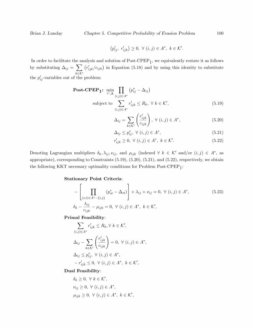
Brian J. Lunday Chapter 5. Competitive Probability of Evasion Problem 100
(p′ij , r
′ijk
)≥ 0, ∀ (i, j) ∈ A∗, k ∈ K′.
In order to facilitate the analysis and solution of Post-CPEP1, we equivalently restate it as followsby substituting ∆ij =
∑k∈K′
(r′ijk/cijk
)in Equation (5.18) and by using this identity to substitute
the p′ij-variables out of the problem:
Post-CPEP1: minr′,∆
∏(i,j)∈A∗
(p∗ij −∆ij
)subject to
∑(i,j)∈A∗
r′ijk ≤ Rk, ∀ k ∈ K′, (5.19)
∆ij =∑k∈K′
(r′ijkcijk
), ∀ (i, j) ∈ A∗, (5.20)
∆ij ≤ p∗ij , ∀ (i, j) ∈ A∗, (5.21)
r′ijk ≥ 0, ∀ (i, j) ∈ A∗, k ∈ K′. (5.22)
Denoting Lagrangian multipliers δk, λij , νij , and ρijk (indexed ∀ k ∈ K′ and/or (i, j) ∈ A∗, asappropriate), corresponding to Constraints (5.19), (5.20), (5.21), and (5.22), respectively, we obtainthe following KKT necessary optimality conditions for Problem Post-CPEP1:
Stationary Point Criteria:
−
∏(s,t)∈A∗−i,j
(p∗st −∆st)
+ λij + νij = 0, ∀ (i, j) ∈ A∗, (5.23)
δk −λij
cijk− ρijk = 0, ∀ (i, j) ∈ A∗, k ∈ K′,
Primal Feasibility:∑(i,j)∈A∗
r′ijk ≤ Rk,∀ k ∈ K′,
∆ij −∑k∈K′
(r′ijkcijk
)= 0, ∀ (i, j) ∈ A∗,
∆ij ≤ p∗ij , ∀ (i, j) ∈ A∗,
− r′ijk ≤ 0, ∀ (i, j) ∈ A∗, k ∈ K′,
Dual Feasibility:
δk ≥ 0, ∀ k ∈ K′,
νij ≥ 0, ∀ (i, j) ∈ A∗,
ρijk ≥ 0, ∀ (i, j) ∈ A∗, k ∈ K′,
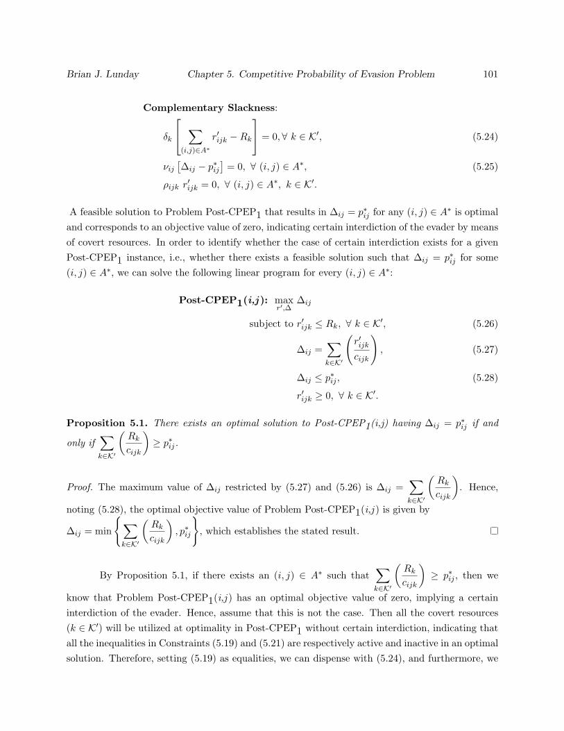
Brian J. Lunday Chapter 5. Competitive Probability of Evasion Problem 101
Complementary Slackness:
δk
∑(i,j)∈A∗
r′ijk −Rk
= 0,∀ k ∈ K′, (5.24)
νij
[∆ij − p∗ij
]= 0, ∀ (i, j) ∈ A∗, (5.25)
ρijk r′ijk = 0, ∀ (i, j) ∈ A∗, k ∈ K′.
A feasible solution to Problem Post-CPEP1 that results in ∆ij = p∗ij for any (i, j) ∈ A∗ is optimaland corresponds to an objective value of zero, indicating certain interdiction of the evader by meansof covert resources. In order to identify whether the case of certain interdiction exists for a givenPost-CPEP1 instance, i.e., whether there exists a feasible solution such that ∆ij = p∗ij for some(i, j) ∈ A∗, we can solve the following linear program for every (i, j) ∈ A∗:
Post-CPEP1(i,j ): maxr′,∆
∆ij
subject to r′ijk ≤ Rk, ∀ k ∈ K′, (5.26)
∆ij =∑k∈K′
(r′ijkcijk
), (5.27)
∆ij ≤ p∗ij , (5.28)
r′ijk ≥ 0, ∀ k ∈ K′.
Proposition 5.1. There exists an optimal solution to Post-CPEP1(i,j) having ∆ij = p∗ij if and
only if∑k∈K′
(Rk
cijk
)≥ p∗ij.
Proof. The maximum value of ∆ij restricted by (5.27) and (5.26) is ∆ij =∑k∈K′
(Rk
cijk
). Hence,
noting (5.28), the optimal objective value of Problem Post-CPEP1(i,j ) is given by
∆ij = min
∑k∈K′
(Rk
cijk
), p∗ij
, which establishes the stated result.
By Proposition 5.1, if there exists an (i, j) ∈ A∗ such that∑k∈K′
(Rk
cijk
)≥ p∗ij , then we
know that Problem Post-CPEP1(i,j ) has an optimal objective value of zero, implying a certaininterdiction of the evader. Hence, assume that this is not the case. Then all the covert resources(k ∈ K′) will be utilized at optimality in Post-CPEP1 without certain interdiction, indicating thatall the inequalities in Constraints (5.19) and (5.21) are respectively active and inactive in an optimalsolution. Therefore, setting (5.19) as equalities, we can dispense with (5.24), and furthermore, we
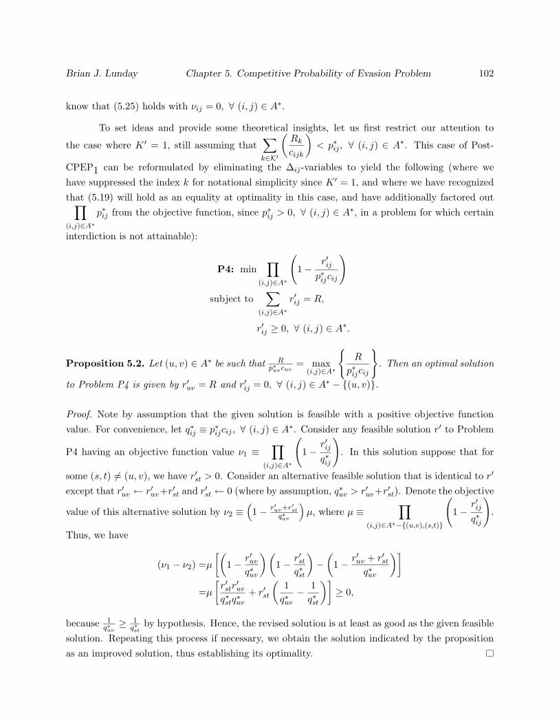
Brian J. Lunday Chapter 5. Competitive Probability of Evasion Problem 102
know that (5.25) holds with νij = 0, ∀ (i, j) ∈ A∗.
To set ideas and provide some theoretical insights, let us first restrict our attention to
the case where K ′ = 1, still assuming that∑k∈K′
(Rk
cijk
)< p∗ij , ∀ (i, j) ∈ A∗. This case of Post-
CPEP1 can be reformulated by eliminating the ∆ij-variables to yield the following (where wehave suppressed the index k for notational simplicity since K ′ = 1, and where we have recognizedthat (5.19) will hold as an equality at optimality in this case, and have additionally factored out∏(i,j)∈A∗
p∗ij from the objective function, since p∗ij > 0, ∀ (i, j) ∈ A∗, in a problem for which certain
interdiction is not attainable):
P4: min∏
(i,j)∈A∗
(1−
r′ijp∗ijcij
)
subject to∑
(i,j)∈A∗
r′ij = R,
r′ij ≥ 0, ∀ (i, j) ∈ A∗.
Proposition 5.2. Let (u, v) ∈ A∗ be such that Rp∗uvcuv
= max(i,j)∈A∗
R
p∗ijcij
. Then an optimal solution
to Problem P4 is given by r′uv = R and r′ij = 0, ∀ (i, j) ∈ A∗ − (u, v).
Proof. Note by assumption that the given solution is feasible with a positive objective functionvalue. For convenience, let q∗ij ≡ p∗ijcij , ∀ (i, j) ∈ A∗. Consider any feasible solution r′ to Problem
P4 having an objective function value ν1 ≡∏
(i,j)∈A∗
(1−
r′ijq∗ij
). In this solution suppose that for
some (s, t) 6= (u, v), we have r′st > 0. Consider an alternative feasible solution that is identical to r′
except that r′uv ← r′uv+r′st and r′st ← 0 (where by assumption, q∗uv > r′uv+r′st). Denote the objective
value of this alternative solution by ν2 ≡(1− r′uv+r′st
q∗uv
)µ, where µ ≡
∏(i,j)∈A∗−(u,v),(s,t)
(1−
r′ijq∗ij
).
Thus, we have
(ν1 − ν2) =µ[(
1− r′uv
q∗uv
)(1− r′st
q∗st
)−(
1− r′uv + r′stq∗uv
)]=µ[r′str
′uv
q∗stq∗uv
+ r′st
(1q∗uv
− 1q∗st
)]≥ 0,
because 1q∗uv≥ 1
q∗stby hypothesis. Hence, the revised solution is at least as good as the given feasible
solution. Repeating this process if necessary, we obtain the solution indicated by the propositionas an improved solution, thus establishing its optimality.
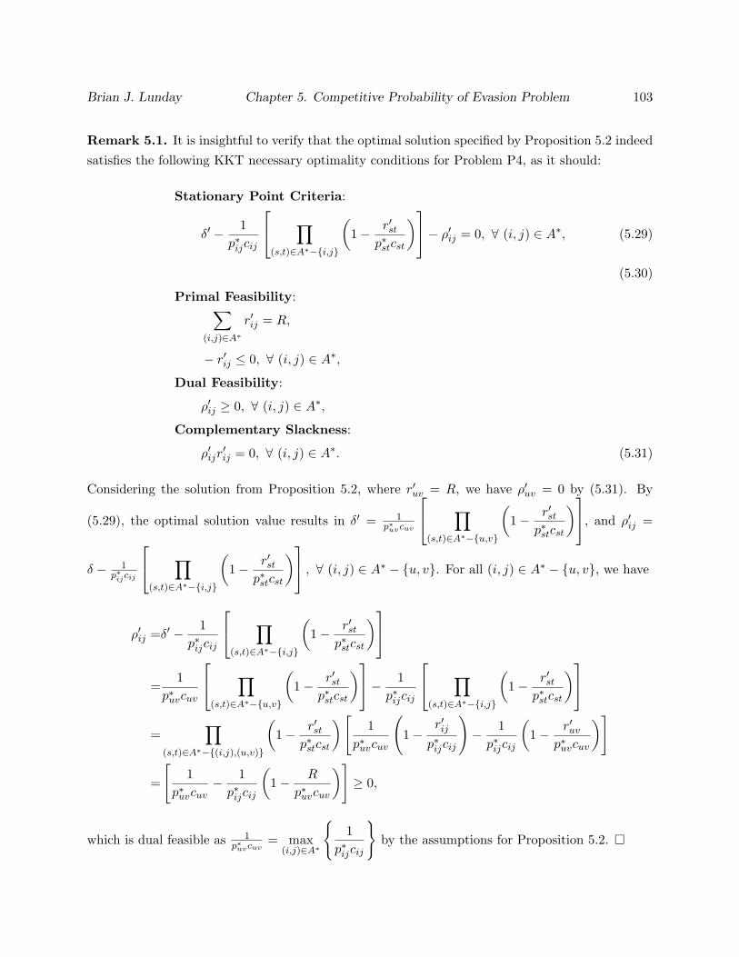
Brian J. Lunday Chapter 5. Competitive Probability of Evasion Problem 103
Remark 5.1. It is insightful to verify that the optimal solution specified by Proposition 5.2 indeedsatisfies the following KKT necessary optimality conditions for Problem P4, as it should:
Stationary Point Criteria:
δ′ − 1p∗ijcij
∏(s,t)∈A∗−i,j
(1− r′st
p∗stcst
)− ρ′ij = 0, ∀ (i, j) ∈ A∗, (5.29)
(5.30)
Primal Feasibility:∑(i,j)∈A∗
r′ij = R,
− r′ij ≤ 0, ∀ (i, j) ∈ A∗,
Dual Feasibility:
ρ′ij ≥ 0, ∀ (i, j) ∈ A∗,
Complementary Slackness:
ρ′ijr′ij = 0, ∀ (i, j) ∈ A∗. (5.31)
Considering the solution from Proposition 5.2, where r′uv = R, we have ρ′uv = 0 by (5.31). By
(5.29), the optimal solution value results in δ′ = 1p∗uvcuv
∏(s,t)∈A∗−u,v
(1− r′st
p∗stcst
), and ρ′ij =
δ − 1p∗ijcij
∏(s,t)∈A∗−i,j
(1− r′st
p∗stcst
) , ∀ (i, j) ∈ A∗ − u, v. For all (i, j) ∈ A∗ − u, v, we have
ρ′ij =δ′ − 1p∗ijcij
∏(s,t)∈A∗−i,j
(1− r′st
p∗stcst
)=
1p∗uvcuv
∏(s,t)∈A∗−u,v
(1− r′st
p∗stcst
)− 1p∗ijcij
∏(s,t)∈A∗−i,j
(1− r′st
p∗stcst
)=
∏(s,t)∈A∗−(i,j),(u,v)
(1− r′st
p∗stcst
)[1
p∗uvcuv
(1−
r′ijp∗ijcij
)− 1p∗ijcij
(1− r′uv
p∗uvcuv
)]
=
[1
p∗uvcuv− 1p∗ijcij
(1− R
p∗uvcuv
)]≥ 0,
which is dual feasible as 1p∗uvcuv
= max(i,j)∈A∗
1
p∗ijcij
by the assumptions for Proposition 5.2.
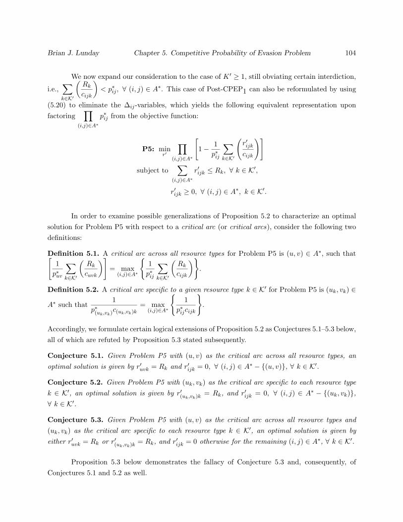
Brian J. Lunday Chapter 5. Competitive Probability of Evasion Problem 104
We now expand our consideration to the case of K ′ ≥ 1, still obviating certain interdiction,
i.e.,∑k∈K′
(Rk
cijk
)< p∗ij , ∀ (i, j) ∈ A∗. This case of Post-CPEP1 can also be reformulated by using
(5.20) to eliminate the ∆ij-variables, which yields the following equivalent representation uponfactoring
∏(i,j)∈A∗
p∗ij from the objective function:
P5: minr′
∏(i,j)∈A∗
[1− 1
p∗ij
∑k∈K′
(r′ijkcijk
)]
subject to∑
(i,j)∈A∗
r′ijk ≤ Rk, ∀ k ∈ K′,
r′ijk ≥ 0, ∀ (i, j) ∈ A∗, k ∈ K′.
In order to examine possible generalizations of Proposition 5.2 to characterize an optimalsolution for Problem P5 with respect to a critical arc (or critical arcs), consider the following twodefinitions:
Definition 5.1. A critical arc across all resource types for Problem P5 is (u, v) ∈ A∗, such that[1p∗uv
∑k∈K′
(Rk
cuvk
)]= max
(i,j)∈A∗
1p∗ij
∑k∈K′
(Rk
cijk
).
Definition 5.2. A critical arc specific to a given resource type k ∈ K′ for Problem P5 is (uk, vk) ∈
A∗ such that1
p∗(uk,vk)c(uk,vk)k= max
(i,j)∈A∗
1
p∗ijcijk
.
Accordingly, we formulate certain logical extensions of Proposition 5.2 as Conjectures 5.1–5.3 below,all of which are refuted by Proposition 5.3 stated subsequently.
Conjecture 5.1. Given Problem P5 with (u, v) as the critical arc across all resource types, anoptimal solution is given by r′uvk = Rk and r′ijk = 0, ∀ (i, j) ∈ A∗ − (u, v), ∀ k ∈ K′.
Conjecture 5.2. Given Problem P5 with (uk, vk) as the critical arc specific to each resource typek ∈ K′, an optimal solution is given by r′(uk,vk)k = Rk, and r′ijk = 0, ∀ (i, j) ∈ A∗ − (uk, vk),∀ k ∈ K′.
Conjecture 5.3. Given Problem P5 with (u, v) as the critical arc across all resource types and(uk, vk) as the critical arc specific to each resource type k ∈ K′, an optimal solution is given byeither r′uvk = Rk or r′(uk,vk)k = Rk, and r′ijk = 0 otherwise for the remaining (i, j) ∈ A∗, ∀ k ∈ K′.
Proposition 5.3 below demonstrates the fallacy of Conjecture 5.3 and, consequently, ofConjectures 5.1 and 5.2 as well.
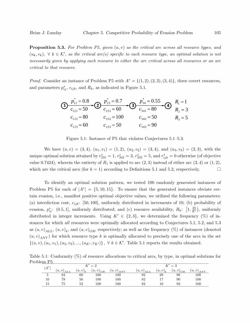
Brian J. Lunday Chapter 5. Competitive Probability of Evasion Problem 105
Proposition 5.3. For Problem P5, given (u, v) as the critical arc across all resource types, and(uk, vk), ∀ k ∈ K′, as the critical arc(s) specific to each resource type, an optimal solution is notnecessarily given by applying each resource to either the arc critical across all resources or an arccritical to that resource.
Proof. Consider an instance of Problem P5 with A∗ = (1, 2), (2, 3), (3, 4), three covert resources,and parameters p∗ij , cijk, and Rk, as indicated in Figure 5.1.
1 42 3
60
80
50
8.0
123
122
121
*
12
c
c
c
p
5
3
1
3
2
1
R
R
R
50
100
60
7.0
233
232
231
*
23
c
c
c
p
90
50
80
55.0
343
342
341
*
34
c
c
c
p
Figure 5.1: Instance of P5 that violates Conjectures 5.1–5.3.
We have (u, v) = (3, 4), (u1, v1) = (1, 2), (u2, v2) = (3, 4), and (u3, v3) = (2, 3), with theunique optimal solution attained by r∗231 = 1, r∗342 = 3, r∗233 = 5, and r∗ijk = 0 otherwise (of objectivevalue 0.7424), wherein the entirety of R1 is applied to arc (2, 3) instead of either arc (3, 4) or (1, 2),which are the critical arcs (for k = 1) according to Definitions 5.1 and 5.2, respectively.
To identify an optimal solution pattern, we tested 100 randomly generated instances ofProblem P5 for each of |A∗| = 5, 10, 15. To ensure that the generated instances obviate cer-tain evasion, i.e., manifest positive optimal objective values, we utilized the following parameters:(a) interdiction cost, cijk: [50, 100], uniformly distributed in increments of 10; (b) probability ofevasion, p∗ij : (0.5, 1], uniformly distributed; and (c) resource availability, Rk:
[1, 25
K′
), uniformly
distributed in integer increments. Using K ′ ∈ 2, 3, we determined the frequency (%) of in-stances for which all resources were optimally allocated according to Conjectures 5.1, 5.2, and 5.3as (u, v)ALL, (u, v)k, and (u, v)OR, respectively; as well as the frequency (%) of instances (denoted(u, v)ANY ) for which resource type k is optimally allocated to precisely one of the arcs in the set(u, v), (u1, v1), (u2, v2), ..., (uK′ , vK′) , ∀ k ∈ K′. Table 5.1 reports the results obtained.
Table 5.1: Conformity (%) of resource allocations to critical arcs, by type, in optimal solutions forProblem P5
|A∗| K′ = 2 K′ = 3(u, v)ALL (u, v)k (u, v)OR (u, v)ANY (u, v)ALL (u, v)k (u, v)OR (u, v)ANY
5 82 60 100 100 92 28 98 10010 78 56 100 100 82 17 90 10015 75 52 100 100 82 16 92 100
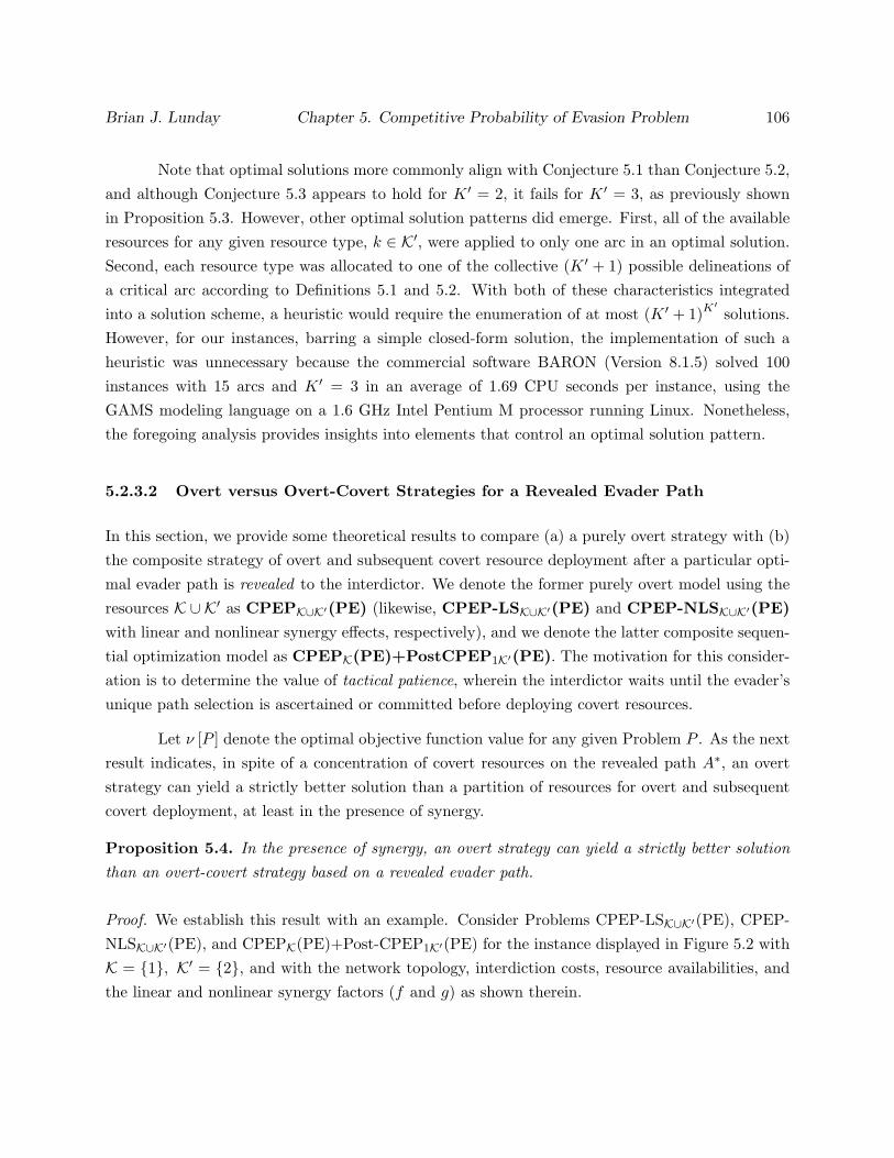
Brian J. Lunday Chapter 5. Competitive Probability of Evasion Problem 106
Note that optimal solutions more commonly align with Conjecture 5.1 than Conjecture 5.2,and although Conjecture 5.3 appears to hold for K ′ = 2, it fails for K ′ = 3, as previously shownin Proposition 5.3. However, other optimal solution patterns did emerge. First, all of the availableresources for any given resource type, k ∈ K′, were applied to only one arc in an optimal solution.Second, each resource type was allocated to one of the collective (K ′ + 1) possible delineations ofa critical arc according to Definitions 5.1 and 5.2. With both of these characteristics integratedinto a solution scheme, a heuristic would require the enumeration of at most (K ′ + 1)K′
solutions.However, for our instances, barring a simple closed-form solution, the implementation of such aheuristic was unnecessary because the commercial software BARON (Version 8.1.5) solved 100instances with 15 arcs and K ′ = 3 in an average of 1.69 CPU seconds per instance, using theGAMS modeling language on a 1.6 GHz Intel Pentium M processor running Linux. Nonetheless,the foregoing analysis provides insights into elements that control an optimal solution pattern.
5.2.3.2 Overt versus Overt-Covert Strategies for a Revealed Evader Path
In this section, we provide some theoretical results to compare (a) a purely overt strategy with (b)the composite strategy of overt and subsequent covert resource deployment after a particular opti-mal evader path is revealed to the interdictor. We denote the former purely overt model using theresources K ∪ K′ as CPEPK∪K′(PE) (likewise, CPEP-LSK∪K′(PE) and CPEP-NLSK∪K′(PE)
with linear and nonlinear synergy effects, respectively), and we denote the latter composite sequen-tial optimization model as CPEPK(PE)+PostCPEP1K′(PE). The motivation for this consider-ation is to determine the value of tactical patience, wherein the interdictor waits until the evader’sunique path selection is ascertained or committed before deploying covert resources.
Let ν [P ] denote the optimal objective function value for any given Problem P . As the nextresult indicates, in spite of a concentration of covert resources on the revealed path A∗, an overtstrategy can yield a strictly better solution than a partition of resources for overt and subsequentcovert deployment, at least in the presence of synergy.
Proposition 5.4. In the presence of synergy, an overt strategy can yield a strictly better solutionthan an overt-covert strategy based on a revealed evader path.
Proof. We establish this result with an example. Consider Problems CPEP-LSK∪K′(PE), CPEP-NLSK∪K′(PE), and CPEPK(PE)+Post-CPEP1K′(PE) for the instance displayed in Figure 5.2 withK = 1, K′ = 2, and with the network topology, interdiction costs, resource availabilities, andthe linear and nonlinear synergy factors (f and g) as shown therein.

Brian J. Lunday Chapter 5. Competitive Probability of Evasion Problem 107
s
1
2
t
100
100
12
11
s
s
c
c
300
300
22
21
s
s
c
c
101
101
21
11
t
t
c
c
301
301
22
12
t
t
c
c 10
2.0
5.0
60
60
2
1
h
g
f
R
R
Figure 5.2: CPEP Instance.
For this example, we obtain ν [CPEP-LSK∪K′(PE)] = 0.625 and ν [CPEP-NLSK∪K′(PE)] =0.545, where an optimal solution to each problem is given by r∗s11 = r∗s12 = 15, r∗s21 = r∗s22 = 45,and r∗ijk = 0 otherwise. On the other hand, Problem CPEPK(PE) is optimized by the allocationscheme r∗∗s11 = 15, r∗∗s21 = 45, and r∗∗1t1 = r∗∗2t1 = 0, leading to a particular revealed evader optimalpath A∗ = (s, 2), (2, t). Consequently, the optimal solution to Post-CPEP1K′(PE) is given byr′∗∗s22 = 60 and r′∗∗2t2 = 0 with ν [CPEPK(PE)+PostCPEP1K′(PE)] = 0.65, which represents a worsesolution than either overt strategy.
Remark 5.2. Whereas the solution to Problem CPEPK(PE) indicated in Proposition 5.4 is unique,there exist two alternatively optimal evader path choices for A∗. Should the evader select A∗ =(s, 1), (1, t), in lieu of the alternative optimal path selected in the proof of Proposition 5.4, thesubsequent optimal solution to Post-CPEP1K′(PE) is given by r′∗∗s12 = 60 and r′∗∗1t2 = 0, whichresults in ν [CPEPK(PE)+PostCPEP1K′(PE)] = 0.25, an improvement over either overt strategy.However, note that both alternatively optimal paths result in a lesser optimal evasion probabilityfor CPEPK(PE)+Post-CPEP1K′(PE) than attained by CPEPK∪K′(PE) without synergy, for whichν [CPEPK∪K′(PE)] = 0.7 upon utilizing optimal resource allocations of r∗s11 = r∗s12 = 15, r∗s21 =r∗s22 = 45, and r∗ijk = 0 otherwise.
In the absence of synergy, the nature of the nonconvex objective function and the possibilityof paths sharing arcs eludes a categorical proof in general as to the relative values of overt versusovert-covert resource deployments with a revealed evader path. However, for the special case ofdisjoint path networks wherein the probability of evasion on each path is a monotone decreasingfunction of simply the total resources assigned, which we henceforth refer to as the MonotoneAllocation Property (MAP), Proposition 5.5 below provides a definitive resolution.
Proposition 5.5. For a revealed evader path on a network having disjoint paths with MAP holdingtrue, we have in the absence of synergy that ν [CPEPK(PE)+PostCPEP1K′(PE)] ≤ ν [CPEPK∪K′(PE)].
Brian J. Lunday Chapter 5. Competitive Probability of Evasion Problem 108
Proof. Consider an optimal solution to Problem CPEPK(PE)+Post-CPEP1K′(PE) given by r∗ijk,∀ (i, j) ∈ A, k ∈ K; a consequent optimal revealed path A∗; along with subsequent resourceallocations r′∗ijk, ∀ (i, j) ∈ A∗, k ∈ K′; thus yielding an evasion probability ofp∗ = ν [CPEPK(PE)+PostCPEP1K′(PE)]. Note that these resource allocations are feasible toProblem CPEPK∪K′(PE). If such resource allocations are also optimal to Problem CPEPK∪K′(PE),then we have ν [CPEPK∪K′(PE)] ≥ p∗ (with ν [CPEPK∪K′(PE)] = p∗ in the case where A∗ gives themaximum probability of evasion over all paths). On the other hand, if these resource allocationsare not optimal to Problem CPEPK∪K′(PE), then a redistribution of resources K ∪ K′ from thesolution to Problem CPEPK(PE)+Post-CPEP1K′(PE) is required to attain optimality to ProblemCPEPK∪K′(PE). If such a redistribution requires decreasing the total allocations to A∗ (or leavingthis total the same), then the probability of evasion on path A∗ will increase (or stay the same),resulting in ν [CPEPK∪K′(PE)] ≥ p∗. Otherwise, assume that the redistribution requires increasingthe total allocations to A∗, which we can suppose occurs via additional reallocations from K.However, for any such redistribution of resources from K, the resulting objective value for theoptimal solution to Problem CPEPK∪K′(PE) evaluated with respect to just the resources K (i.e.,applying only the resources from K to allocations as determined by an optimal solution to ProblemCPEPK∪K′(PE)) is p ≥ ν [CPEPK(PE)] ≥ p∗. But p is realized on a path Π 6= A∗ becausethe hypothesized requirement to increase the total resource allocations to A∗ from K results in aprobability of evasion on A∗ with respect to resources K to be strictly less than ν [CPEPK(PE)],whereas p ≥ ν [CPEPK(PE)] from above. Moreover, because of the assumed disjoint paths, theaddition of the resources in K′ (to A∗) in the solution to CPEPK∪K′(PE) does not affect the pathΠ. Hence, the optimal value of Problem CPEPK∪K′(PE) is p ≥ p∗.
Note that the hypothesis (and proof) of Proposition 5.5 is predicated on the MAP, whereinthe evasion probability on any path is a monotone decreasing function of the total resource allo-cation, irrespective of the individual types of resources comprising this total. The following resultand its corollary identify possible conditions under which MAP would hold.
Proposition 5.6. Suppose that cijk ≡ cij , ∀ (i, j) ∈ A, k ∈ K. Then MAP holds true.
Proof. It is sufficient to show that the evasion probability pij for any arc (i, j) ∈ A in CPEP is amonotone decreasing function of simply the total resource allocations, because then for any path Π,the minimal value of
∏(i,j)∈Π
pij would also be a monotone decreasing function of the total resources
allocated to Π. Under the conditions of the proposition, we get
pij = 1−∑k∈K
(rijkcijk
)= 1− 1
cij
(∑k∈K
rijk
), ∀ (i, j) ∈ A,

Brian J. Lunday Chapter 5. Competitive Probability of Evasion Problem 109
which establishes the desired result.
Corollary 5.1. Suppose that cijk = αk, ∀ (i, j) ∈ A, k ∈ K. Then the resource availabilities inProblem CPEP can be scaled to ensure that MAP holds true.
Proof. Under the condition of the corollary, we have pij = 1−∑k∈K
(rijkαk
). By substituting rS
ijk ≡
rijkαk
, ∀ (i, j) ∈ A, k ∈ K, and RSk =
Rk
αk, ∀ k ∈ K, we get pij = 1 −
∑k∈K
rSijk, ∀ (i, j) ∈ A, where
the resource availability constraints in Problem CPEP can be scaled to yield∑(i,j)∈A
rSijk ≤ RS
k , ∀ k ∈ K, with rSijk ≥ 0, ∀ (i, j) ∈ A, k ∈ K.
Hence, by the proof of Proposition 5.6, the scaled problem CPEP satisfies MAP.
Remark 5.3. We may also consider revised models wherein we assume that the resource allocationsare restricted to be integer-valued. Denote such corresponding models as CPEPK∪K′(PE-I),CPEP-LSK∪K′(PE-I), CPEP-NLSK∪K′(PE-I), and CPEPK(PE-I)+PostCPEP1K′(PE-I).These models might be particularly relevant when deploying certain types of indivisible resources,especially when such resources are available in relatively small quantities so that rounding anoptimal solution to a continuous relaxation might be inadequate. Propositions 5.4–5.6 also holdunder integrality restrictions for resource allocations, via the identical proofs as stated.
5.2.3.3 Covert Resource Deployment on Multiple Unrevealed Optimal Evader Paths
Now, consider the case when the deployment of overt resources results in more than one alternativeoptimal path for the evader to traverse, and where the actual choice is not a priori revealed. Sincethe evader’s selection of a path to traverse is not uniquely evident, we must consider all such pathsfor covert resource deployment. Denote A∗ ≡(i, j) ∈ A : arc (i, j) is part of some optimal solutionto Problem CPEP. Note that determining A∗ is a potentially exponential task (we discuss thisfurther in Section 5.3). We formulate the resulting problem Post-CPEP as follows:
Post-CPEP: minr′, p′
maxx′
∏(i,j)∈A∗
(1− x′ij + p′ijx
′ij
)
subject to∑
j:(i,j)∈A∗x′ij −
∑j:(j,i)∈A∗
x′ji =
1 if i = s
0 if i 6= s, t
−1 if i = t
, ∀ i ∈ N,
∑(i,j)∈A∗
r′ijk ≤ Rk, ∀ k ∈ K′,

Brian J. Lunday Chapter 5. Competitive Probability of Evasion Problem 110
p′ij = p∗ij −∑k∈K
(r′ijkcijk
), ∀ (i, j) ∈ A∗, (5.32)
x′ij ∈ 0, 1 , ∀ (i, j) ∈ A∗,(p′ij , r
′ijk
)≥ 0, ∀ (i, j) ∈ A∗, k ∈ K′.
This formulation for deploying covert resources is nearly identical to that of Problem CPEP, ex-cept that the arc-set considered is restricted to A∗, and the arcs are partially interdicted prior tocovert resource deployment, as evidenced by the p∗ij-variable values in Constraint (5.32), which areobtained via the given optimal solution to Problem CPEP . The minimax problem Post-CPEPcan also be reformulated as an optimization problem Post-CPEP(PE) similar to CPEP(PE),by enumerating the alternative optimal evader paths as identified via the active constraints (5.14)in an optimal solution to Problem CPEP(PE). We denote the composite sequential optimizationmodel involving the deployment of the overt resources (K) followed by the covert resources (K′) asCPEPK(PE)+PostCPEPK′(PE), and likewise denote the composite model that further imposesintegrality retrictions on resource allocations as CPEPK(PE-I)+PostCPEPK′(PE-I).
5.3 Computational Results
In this section, we conduct a comparative empirical analysis for a two-resource problem (K = 1 andK ′ = 1), both with and without integrality restrictions on resource allocations, and for the threemodeling strategies that deploy resources overtly (a) in the absence of synergy; (b) with synergybounded by Constraint (5.10); and (c) with synergy bounded by Constraint (5.12); as well as for thefourth strategy that (d) deploys the set of resources K overtly, and subsequently deploys the set ofresources K′ covertly on a subset of the network defined by A∗ as identified via an optimal solutionto Problem CPEPK(PE) or CPEPK(PE-I), as appropriate. The goal of this experimentation is toempirically identify conditions under which the composite overt-covert use of resources representsa degradation or improvement over the purely overt utilization of all resources, whether with orwithout linear or concave synergy. All runs reported below have been made on a 1.6 GHz IntelPentium M processor computer running Linux, using the GAMS modeling language to run thecommercial software BARON (Version 8.1.5), which further invokes CPLEX (Version 11.1) to solveLP subproblems, and SNOPT (Version 7.2-4) to solve NLP subproblems.
For our analyses, we maintain the topology and network parameters as outlined in Section4.2.3, with the following three exceptions:

Brian J. Lunday Chapter 5. Competitive Probability of Evasion Problem 111
1. Linear synergy factor, f = 0.5: This allows for a maximum of 20% probability of detection dueto synergy, when sufficient resources are applied to an arc to ensure certain detection.
2. Nonlinear synergy factor, g = 0.2: This also imposes a maximum of 20% probability of detectionon any arc due to synergy, under conditions of certain detection.
3. Nonlinear synergy scaling factor, h = 10: This affects a concavity to the synergistic relationshipto ensure that CPEP-NLSK∪K′(PE) will determine improved solutions over CPEP-LSK∪K′(PE),but with equal synergy on any arc that manifests either certain probabilty of detection orcertain probability of evasion. This parameter is set to facilitate a uniform comparison of bothsynergistic formulations to CPEPK(PE)+Post-CPEPK′(PE), and not particularly to each other.
4. Resource availability, Rk: We select Rk ∈ d1, RMAXe , ∀ k ∈ K ∪K′, uniformly distributed overinteger values, where
RMAX =
0.8m
min(i,j)∈Ak∈K∪K′
cijk
K +K ′ .
Barring a column generation scheme, the path-enumeration approach adopted herein forthe principal purpose of providing insights into the effects of strategic decisions requires identifyingall s − t paths, l ∈ L. Considering the topography displayed in Figure 4.2, an m × n networkwill manifest |L| ≤ (3m)(n−1). Due to this exponential complexity, we will limit our computationalanalysis to networks of size (m,n) = (4, 4), for which |L| = 1000 (increasing (m,n) to (5, 5) results in|L| = 28561, for which instances of CPEP-NLS(PE) require more than 3600 CPU seconds to solve toglobal optimality with BARON). Furthermore, the CPEP(PE) formulation is a nonconvex programdue to Constraint (5.14) and, as such, this problem and its variants require a robust commercialsolver to ensure global optimality. Note that, as mentioned previously, this nonconvexity wouldremain an impediment in a relaxation approach in which the constraints (5.14) are (partially)relaxed and are iteratively generated in an as-and-when-needed fashion.
5.3.1 Revealed Optimal Evader Path
In this section, we assume that a single optimal evader path is revealed to the interdictor priorto the deployment of covert resources, and we compare the four strategies under assumptions ofeither continuous or integer-restricted resource allocations. Define π to be an attenuation multiplierfor resource availability (e.g., when π = 0.75, all resource availabilities are reduced by 25%). Wefirst consider continuous resource allocations and examine the effect of the relative and absoluteavailabilities of resources on the relative performance of CPEPK(PE)+Post-CPEP1K′(PE) com-pared to strategies embodied by CPEPK∪K′(PE), CPEP-LSK∪K′(PE), and CPEP-NLSK∪K′(PE),

Brian J. Lunday Chapter 5. Competitive Probability of Evasion Problem 112
with γ ≡ R2R1∈
14 ,
12 , 1, 2, 4
and π ∈
1, 1
2 ,14 ,
18
on a 3×3 network, setting cij1 = cij2, ∀ (i, j) ∈ A
(see Proposition 5.6). In our test, the evader’s selection of the path to traverse was deter-mined randomly and with equal probability among the alternative optimal paths resulting fromthe overt resource deployment. (Were an evader concerned about the possibility of covert in-terdictor resources being deployed, this assumption would no longer hold as the evader’s pathselection would be more deliberate.) We terminated the algorithms based on a relative toler-ance of 10−4 or 1800 CPU seconds of effort. Table 5.2 reports the average relative gaps (%)between ν [CPEPK(PE)+Post-CPEP1K′(PE)] and ν [CPEPK∪K′(PE)], ν [CPEP-LSK∪K′(PE)], andν [CPEP-NLSK∪K′(PE)], for each (γ, π)-combination, along with the number of instances out of 30(specified in parentheses) for which the CPEPK(PE)+Post-CPEP1K′(PE) strategy was at least asgood.
Table 5.2: Average Relative Gap (%) and Number of Instances (Out of 30) Which Result inν [CPEPK(PE)+PostCPEP1K′(PE)] ≤ ν[P] for Different Overt Problems P.
γ π CPEPK∪K′(PE) CPEP-LSK∪K′(PE) CPEP-NLSK∪K′(PE)1 -79.885 (30) -79.148 (30) -77.712 (30)
1/41/2 -55.184 (30) -54.238 (30) -52.250 (30)1/4 -30.441 (30) -29.691 (30) -27.930 (30)1/8 -14.065 (30) -13.587 (30) -12.415 (30)1 -89.285 (30) -88.972 (30) -88.295 (30)
1/21/2 -70.722 (30) -69.876 (30) -68.197 (30)1/4 -46.662 (30) -45.766 (30) -43.727 (30)1/8 -25.357 (30) -24.682 (30) -23.011 (30)1 -92.680 (30) -89.093 (30) -91.877 (30)
11/2 -81.991 (30) -81.356 (30) -80.127 (30)1/4 -60.468 (30) -59.569 (30) -57.633 (30)1/8 -36.951 (30) -36.121 (30) -34.111 (30)1 -94.684 (30) -94.566 (30) -94.279 (30)
21/2 -89.340 (30) -89.195 (30) -88.823 (30)1/4 -71.320 (30) -70.937 (30) -70.061 (30)1/8 -45.975 (30) -45.528 (30) -44.416 (30)1 -96.075 (30) -96.026 (30) -95.895 (30)
41/2 -91.029 (30) -90.963 (30) -90.781 (30)1/4 -75.990 (30) -75.811 (30) -75.387 (30)1/8 -52.819 (30) -52.596 (30) -52.043 (30)
π = 1 -90.522 (30) -89.561 (30) -89.612 (30)
Averagesπ = 1/2 -77.653(30) -77.126 (30) -76.035 (30)π = 1/4 -56.976 (30) -56.355 (30) -54.948 (30)π = 1/8 -35.033 (30) -34.503 (30) -33.199 (30)
In the presence of a revealed evader path, the subsequent deployment of the resource K′
covertly results in a significant improvement in the optimal objective value compared to the overtstrategies, with the magnitude of the average relative gaps generally increasing with increases ineither the relative (γ) or total (π) resource parameters. For none of the instances examined wasthe covert strategy inferior to an overt deployment of resources. This is supported theoreticallyby Propositions 5.5 and 5.6 for the case of CPEPK∪K′(PE), but not necessarily so for the synergy-based models CPEP-LSK∪K′(PE) and CPEP-NLSK∪K′(PE), as exhibited by Proposition 5.4. (For(γ, π) = (1, 1), we encountered one instance when CPEP-LSK∪K′(PE) produced an equivalent

Brian J. Lunday Chapter 5. Competitive Probability of Evasion Problem 113
solution in which the optimal objective value reflected certain detection of the evader.)
Imposing integer restrictions on resource allocations, we repeated the computational testsusing 30 instances each for the same combinations of (γ, π)-parameters along with the same termina-tion criteria. Table 5.3 reports the relative gaps (%) and the number of instances out of 30 (specifiedin parentheses) for which the CPEPK(PE-I)+Post-CPEP1K′(PE-I) strategy was at least as goodas the purely overt strategies CPEPK∪K′(PE-I), CPEP-LSK∪K′(PE-I), and CPEP-NLSK∪K′(PE-I).
Table 5.3: Average Relative Gap (%) and Number of Instances (Out of 30) Which Result inν [CPEPK(PE-I)+PostCPEP1K′(PE-I)] ≤ ν[P] for Different Overt Problems P.
γ π CPEPK∪K′(PE-I) CPEP-LSK∪K′(PE-I) CPEP-NLSK∪K′(PE-I)1 -72.804 (30) -71.853 (30) -71.376 (30)
1/41/2 -49.314 (30) -48.013 (30) -48.926 (30)1/4 -25.904 (30) -25.121 (30) -25.596 (30)1/8 -13.138 (30) -12.744 (30) -12.468 (30)1 -84.160 (30) -83.720 (30) -83.390 (30)
1/21/2 -62.216 (30) -61.236 (30) -60.807 (30)1/4 -42.808 (30) -42.459 (30) -41.946 (30)1/8 -20.982 (30) -20.753 (30) -21.180 (30)1 -90.798 (30) -90.241 (30) -90.078 (30)
11/2 -72.173 (30) -71.657 (30) -70.328 (30)1/4 -53.486 (30) -52.920 (30) -51.847 (30)1/8 -28.385 (30) -28.191 (30) -27.908 (30)1 -94.093 (30) -94.032 (30) -93.922 (30)
21/2 -84.867 (30) -84.680 (30) -84.843 (30)1/4 -68.973 (30) -68.859 (30) -68.776 (30)1/8 -42.747 (30) -42.735 (30) -43.004 (30)1 -95.209 (30) -95.212 (30) -95.236 (30)
41/2 -87.597 (30) -87.377 (30) -87.445 (30)1/4 -74.173 (30) -73.970 (30) -74.361 (30)1/8 -55.496 (30) -55.344 (30) -55.268 (30)
π = 1 -87.413 (30) -87.012 (30) -86.800 (30)
Averagesπ = 1/2 -71.234 (30) -70.593 (30) -70.470 (30)π = 1/4 -53.069 (30) -52.666 (30) -52.505 (30)π = 1/8 -32.150 (30) -31.954 (30) -31.966 (30)
For integer-restricted resource allocations in the presence of a revealed path, the strategyof employing one resource covertly remains markedly superior to all overt strategies for all (γ, π)-combinations, and in no instance examined did it result in a greater optimal objective functionvalue. The only instance for which we found all strategies to be equivalent occurred with (γ, π) =(1/4, 1/8), wherein there was less than one integer unit of each resource type available, resultingtrivially in no deployment of resources for any strategy and certain evasion from detection. Moreimportantly, we note from Tables 5.2 and 5.3 that the average relative gaps are smaller in magnitudewhen resource allocations are restricted to integer values, due to a reduction in resource utilization.
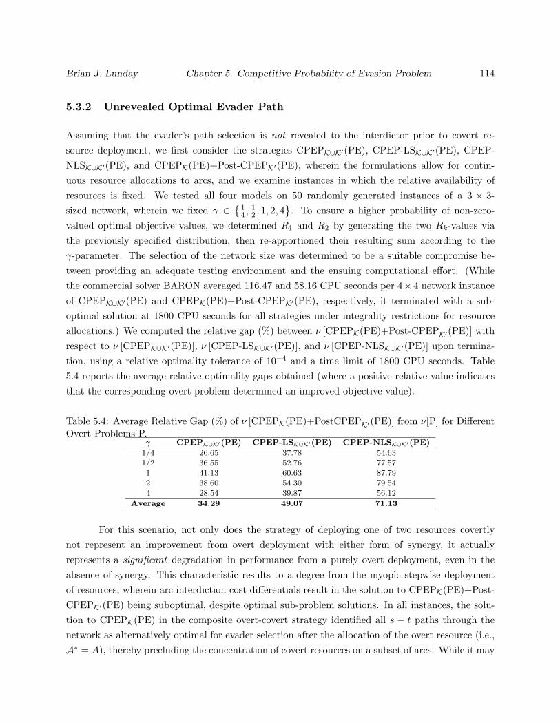
Brian J. Lunday Chapter 5. Competitive Probability of Evasion Problem 114
5.3.2 Unrevealed Optimal Evader Path
Assuming that the evader’s path selection is not revealed to the interdictor prior to covert re-source deployment, we first consider the strategies CPEPK∪K′(PE), CPEP-LSK∪K′(PE), CPEP-NLSK∪K′(PE), and CPEPK(PE)+Post-CPEPK′(PE), wherein the formulations allow for contin-uous resource allocations to arcs, and we examine instances in which the relative availability ofresources is fixed. We tested all four models on 50 randomly generated instances of a 3 × 3-sized network, wherein we fixed γ ∈
14 ,
12 , 1, 2, 4
. To ensure a higher probability of non-zero-
valued optimal objective values, we determined R1 and R2 by generating the two Rk-values viathe previously specified distribution, then re-apportioned their resulting sum according to theγ-parameter. The selection of the network size was determined to be a suitable compromise be-tween providing an adequate testing environment and the ensuing computational effort. (Whilethe commercial solver BARON averaged 116.47 and 58.16 CPU seconds per 4× 4 network instanceof CPEPK∪K′(PE) and CPEPK(PE)+Post-CPEPK′(PE), respectively, it terminated with a sub-optimal solution at 1800 CPU seconds for all strategies under integrality restrictions for resourceallocations.) We computed the relative gap (%) between ν [CPEPK(PE)+Post-CPEPK′(PE)] withrespect to ν [CPEPK∪K′(PE)], ν [CPEP-LSK∪K′(PE)], and ν [CPEP-NLSK∪K′(PE)] upon termina-tion, using a relative optimality tolerance of 10−4 and a time limit of 1800 CPU seconds. Table5.4 reports the average relative optimality gaps obtained (where a positive relative value indicatesthat the corresponding overt problem determined an improved objective value).
Table 5.4: Average Relative Gap (%) of ν [CPEPK(PE)+PostCPEPK′(PE)] from ν[P] for DifferentOvert Problems P.
γ CPEPK∪K′(PE) CPEP-LSK∪K′(PE) CPEP-NLSK∪K′(PE)
1/4 26.65 37.78 54.631/2 36.55 52.76 77.571 41.13 60.63 87.792 38.60 54.30 79.544 28.54 39.87 56.12
Average 34.29 49.07 71.13
For this scenario, not only does the strategy of deploying one of two resources covertlynot represent an improvement from overt deployment with either form of synergy, it actuallyrepresents a significant degradation in performance from a purely overt deployment, even in theabsence of synergy. This characteristic results to a degree from the myopic stepwise deploymentof resources, wherein arc interdiction cost differentials result in the solution to CPEPK(PE)+Post-CPEPK′(PE) being suboptimal, despite optimal sub-problem solutions. In all instances, the solu-tion to CPEPK(PE) in the composite overt-covert strategy identified all s − t paths through thenetwork as alternatively optimal for evader selection after the allocation of the overt resource (i.e.,A∗ = A), thereby precluding the concentration of covert resources on a subset of arcs. While it may

Brian J. Lunday Chapter 5. Competitive Probability of Evasion Problem 115
be argued that the deployment of overt and covert resources should be better coordinated in a solu-tion procedure to deliberately ensure a smaller number of optimal evader paths, such an approachwould result in a noticeably sub-optimal allocation of overt resources for Problem CPEPK(PE)in the first stage, thereby providing the evader with intelligence that additional covertly-deployedresources do exist, and the assumptions made regarding evader path-selection would no longerhold. Although γ does not affect the relative performances in an identifiable manner, we retainthis stratification in further testing in the event that it is significant when other relevant factorsare isolated.
Remark 5.4. To determine if the correlation of the cijk-values between the two resources (denotedas rcosts) affects the relative values of the optimal solutions to CPEPK∪K′(PE) andCPEPK(PE)+ Post-CPEPK′(PE), we tested 50 randomly generated instances each on the networksizes (m,n) ∈ (2, 2), (3, 3), (4, 4) and over the relative resource availabilities γ ∈
14 ,
12 , 1, 2, 4
.
Table 5.5 reports correlations between rcosts and the relative gaps between ν [CPEPK∪K′(PE)] andν [CPEPK(PE)+Post-CPEPK′(PE)] for each problem size-γ combination.
Table 5.5: Correlation between rcosts and relative gaps (%) between ν [CPEPK∪K′(PE)] andν [CPEPK(PE)+Post-CPEPK′(PE)].
γNetwork Size, (m, n)
(2, 2) (3, 3) (4, 4)
1/4 -0.248 -0.097 -0.0831/2 -0.323 -0.133 -0.0861 -0.313 -0.218 -0.0782 -0.382 -0.205 -0.0644 -0.274 -0.107 -0.007
Average -0.308 -0.152 -0.064
The negative correlations indicate that, as rcosts increases, we generally encounter smallerrelative discrepancies between ν [CPEPK(PE)+Post-CPEPK′(PE)] and ν [CPEPK∪K′(PE)]. Al-though the relative availability of resources does not demonstrably affect this correlation, the effectof rcosts on the relative optimality gaps declines with an increase in network size, most likelydue to the reduced influence of any single arc having a significant differential in resource-specificinterdiction costs on the overall solution.
To further isolate the parametric conditions that affect the relative advantage (or disadvan-tage) of deploying one resource covertly, we fixed the cost ratios to establish an absolute positivecorrelation (rcosts = 1), setting µ = cij1
cij2∈
12 , 1, 2
, ∀ (i, j) ∈ A. As before, we tested all four
models on 50 randomly generated instances of a 3 × 3-sized network, wherein γ ∈
14 ,
12 , 1, 2, 4
.
Table 5.6 reports the average relative optimality gaps obtained under these parametric resource-and-cost-ratio combinations, and the final rows indicate the relative effect of a fixed cost ratio, µ,independent of the resource ratio, γ.
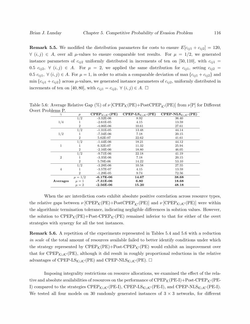
Brian J. Lunday Chapter 5. Competitive Probability of Evasion Problem 116
Remark 5.5. We modified the distribution parameters for costs to ensure E[cij1 + cij2] = 120,∀ (i, j) ∈ A, over all µ-values to ensure comparable test results. For µ = 1/2, we generatedinstance parameters of cij2 uniformly distributed in increments of ten on [50, 110], with cij1 =0.5 cij2, ∀ (i, j) ∈ A. For µ = 2, we applied the same distribution for cij1, setting cij2 =0.5 cij1, ∀ (i, j) ∈ A. For µ = 1, in order to attain a comparable deviation of max cij1 + cij2 andmin cij1 + cij2 across µ-values, we generated instance parameters of cij2, uniformly distributed inincrements of ten on [40, 80], with cij1 = cij2, ∀ (i, j) ∈ A.
Table 5.6: Average Relative Gap (%) of ν [CPEPK(PE)+PostCPEPK′(PE)] from ν[P] for DifferentOvert Problems P.
γ µ CPEPK∪K′(PE) CPEP-LSK∪K′(PE) CPEP-NLSK∪K′(PE)1/2 -3.32E-06 8.92 36.40
1/4 1 -2.61E-05 4.15 13.592 -4.06E-06 10.61 27.61
1/2 -1.31E-05 13.48 44.141/2 1 -7.34E-06 7.18 20.15
2 5.62E-07 22.62 41.611/2 -1.44E-06 18.21 44.12
1 1 6.32E-07 11.32 25.942 -2.16E-06 18.80 46.05
1/2 -9.71E-06 22.18 41.192 1 -3.35E-06 7.18 20.15
2 5.78E-06 14.22 53.101/2 -3.28E-06 10.58 27.55
4 1 -3.57E-07 4.15 13.592 -1.29E-05 9.74 72.56
µ = 1/2 -6.17E-06 14.67 38.68Averages µ = 1 -7.31E-06 6.80 18.68
µ = 2 -2.56E-06 15.20 48.18
When the arc interdiction costs exhibit absolute positive correlation across resource types,the relative gaps between ν [CPEPK(PE)+PostCPEPK′(PE)] and ν [CPEPK∪K′(PE)] were withinthe algorithmic termination tolerance, indicating negligible differences in solution values. However,the solution to CPEPK(PE)+Post-CPEPK′(PE) remained inferior to that for either of the overtstrategies with synergy for all the test instances.
Remark 5.6. A repetition of the experiments represented in Tables 5.4 and 5.6 with a reductionin scale of the total amount of resources available failed to better identify conditions under whichthe strategy represented by CPEPK(PE)+Post-CPEPK′(PE) would exhibit an improvement overthat for CPEPK∪K′(PE), although it did result in roughly proportional reductions in the relativeadvantages of CPEP-LSK∪K′(PE) and CPEP-NLSK∪K′(PE).
Imposing integrality restrictions on resource allocations, we examined the effect of the rela-tive and absolute availabilities of resources on the performance of CPEPK(PE-I)+Post-CPEPK′(PE-I) compared to the strategies CPEPK∪K′(PE-I), CPEP-LSK∪K′(PE-I), and CPEP-NLSK∪K′(PE-I).We tested all four models on 30 randomly generated instances of 3 × 3 networks, for different

Brian J. Lunday Chapter 5. Competitive Probability of Evasion Problem 117
values of the combination of relative resource availabilities given by γ ∈
14 ,
12 , 1, 2, 4
, and ab-
solute resource availabilities given by π ∈1, 1
2 ,14 ,
18
. We set cij1 = cij2, ∀ (i, j) ∈ A (thereby
ensuring rcosts = 1), noting that we are trying to determine the most favorable conditions forthe strategy represented by CPEPK(PE-I)+Post-CPEPK′(PE-I) (see Propositions 5.5 and 5.6 re-lated to revealed paths). Table 5.7 reports the average number of alternatively optimal evaderpaths (out of 49), denoted |L∗|, considered for the deployment of covert resources in Problem Post-CPEPK′(PE-I), and the average relative gaps (%) between ν [CPEPK(PE-I)+Post-CPEPK′(PE-I)]and ν [CPEPK∪K′(PE-I)], ν [CPEP-LSK∪K′(PE-I)], and ν [CPEP-NLSK∪K′(PE-I)], respectively, foreach (γ, π)-combination. We also present in parentheses next to each average relative gap the num-ber of instances (out of 30) for which the CPEPK(PE-I)+Post-CPEPK′(PE-I) strategy was at leastas good. Also, the final row presents the overall average relative gaps (%) for each π-value, alongwith the corresponding ranges for these gaps.
Table 5.7: Average Number of Paths for Covert Resource Deployment, Relative Gap (%) andNumber of Instances ν [CPEPK(PE-I)+PostCPEPK′(PE-I)] ≤ ν[P] for Different Overt ProblemsP.
γ π |L∗| CPEPK∪K′(PE-I) CPEP-LSK∪K′(PE-I) CPEP-NLSK∪K′(PE-I)
1 19.17 -25.894 (28) -18.347 (23) -17.339 (20)
1/41/2 17.5 -7.361 (28) -4.999 (24) -6.725 (26)1/4 19.4 -3.007 (27) -1.827 (23) -2.720 (23)1/8 15.73 -2.727 (30) -2.272 (28) -1.922 (25)
1 18.23 -43.572 (28) -34.915 (26) -31.248 (25)
1/21/2 15.77 -20.192 (29) -17.073 (26) -15.541 (23)1/4 16.27 -9.469 (27) -8.742 (24) -8.033 (25)1/8 15.23 -3.277 (28) -3.078 (28) -3.539 (29)
1 14.17 -59.126 (28) -51.713 (26) -48.162 (26)
11/2 15.87 -25.875 (29) -22.711 (27) -17.181 (25)1/4 14.1 -13.986 (29) -12.724 (29) -10.378 (25)1/8 19.13 -4.573 (29) -4.360 (29) -4.006 (26)
1 14.43 -67.272 (30) -63.909 (28) -61.210 (27)
21/2 14.9 -40.527 (29) -38.671 (28) -38.034 (27)1/4 16.3 -19.632 (28) -19.028 (28) -18.946 (26)1/8 26.8 -6.278 (26) -6.240 (26) -6.812 (26)
1 19.13 -61.973 (29) -59.797 (26) -56.783 (26)
41/2 16 -43.365 (29) -42.253 (29) -41.830 (29)1/4 25.1 -17.763 (25) -16.922 (23) -17.696 (24)1/8 40.63 -3.030 (19) -2.755 (17) -2.220 (16)
π = 1 17.03-51.567 (28.6) -45.736 (25.8) -42.948 (24.8)[-100.00, 6.25] [-100.00, 60.00] [-100.00, 90.52]
Averages π = 1/2 16.01-27.464 (28.8) -25.141 (26.8) -23.862 (26)
and Ranges[-100.00, 3.03] [-100.00, 12.90] [-100.00, 24.16]
π = 1/4 18.23-12.771 (27.2) -11.849 (25.4) -11.554 (24.6)[-92.57, 3.64] [-92.47, 4.35] [-92.80, 10.85]
π = 1/8 23.51-3.977 (26.4) -3.741 (25.6) -3.700 (24.4)[-30.67, 4.17] [-30.36, 5.26] [-28.14, 3.64]
First, note that imposing integrality restrictions on resource allocations results in |L∗| < |L|(on average) for strategy CPEPK(PE-I)+Post-CPEPK′(PE-I), with a 61.85% reduction in the num-

Brian J. Lunday Chapter 5. Competitive Probability of Evasion Problem 118
ber of paths in L∗ relative to L over the 480 instances examined. Although a fewer number of pathsconsidered for covert resource deployment (|L∗|) for a given instance does allow for a greater concen-tration of such resources, it does not necessarily predicate a greater magnitude of the relative gap bythe covert deployment strategy over a purely overt strategy when compared to another instance withsimply a higher |L∗|-value. Indeed, the relative performance gaps are sufficiently influenced by otherinstance parameters so as to preclude generalization. With integer-restricted resource allocations,in contrast to the previous results, the CPEPK(PE-I)+Post-CPEPK′(PE-I) strategy turned out tobe superior to all overt strategies on average, with the relative gaps generally decreasing in magni-tude as the overt strategies transition from CPEPK∪K′(PE-I) to CPEP-LSK∪K′(PE-I) and CPEP-NLSK∪K′(PE-I). The magnitude of the average relative gaps also decline with a decrease in the to-tal availabilities of resource types for each overt strategy. The CPEPK(PE-I)+Post-CPEPK′(PE-I)strategy demonstrated superior results on most instances among the (γ, π)-combinations examined;however, the frequency of instances for which CPEPK(PE-I)+Post-CPEPK′(PE-I) was superior didnot exhibit an identifiable trend across γ- or π-parameters, nor across the overt strategies consid-ered. As the optimal objective value for any of the strategic solutions is bounded by [0, 1], ourranges are significantly greater for higher π-values because the probability of evasion in an optimalsolution is closer to zero. However, the magnitudes of the minimum and maximum relative gapsboth generally increase with π, although no such characterization is discernible across γ-valuesor deployment strategies. Given integer-restricted resource allocations and absolute positive cor-relation of arc-specific detection costs across resource types, we may conclude that deploying aresource covertly and forgoing the opportunity for synergy will likely result in a higher probabilityof detecting an evader, with potentially greater relative benefits under larger resource availabilities.
Note that the integer-restricted formulations with a revealed evader path enabled superiorrelative solutions for the overt-covert resource utilization strategy as reported in Table 5.3, com-pared to the integer-restricted formulations without a revealed path (as reported in Table 5.7),due to the further reduction of the subset of arcs to |L∗| = 1 considered for covert resource allo-cation. Hence, the results empirically exhibit the value of tactical patience, wherein yet greaterrelative benefits may be attained by determining the evader’s path to concentrate covert resourceallocations.
5.3.3 Computational Complexity and Potential Modifications for Implementa-
tion
Although this study provides useful theoretical and empirical results, the scope of testing has beenlimited to moderately-sized networks, both due to the potentially exponential number of directedacyclic paths through larger networks (e.g., for the network topology in Figure 4.2), and due to the
Brian J. Lunday Chapter 5. Competitive Probability of Evasion Problem 119
nonconvex mixed-integer nonlinear programming model formulations for which we have utilized thecommercial software BARON to attain global optimal solutions. However, there exist alternativemodeling variations to address these two features (aside from the aforementioned column generationstrategy) that can enable consideration of larger networks, and we discuss two such variants here.
First, we note that, although transportation networks may exhibit structures similar tothat shown in Figure 4.2, a full enumeration of directed acyclic paths through the network maynot be necessary, much less appropriate. Our consideration of every such path in testing includesmany that do not make practical sense, e.g., the path that travels up (or down) the height of eachcolumn, from the second through the second-to-last column in the transshipment matrix, beforemoving laterally to the next column. Were we to maintain the current network connectivity butonly allow a path to move vertically (up or down) a distance of at most one node within a columnbefore transiting to the next column of the transshipment matrix, the modified enumeration of theset of such paths, LM , would be bounded by |LM | ≤ m(3)(2n−3) for anm×n network and would thusreduce the number of paths considered for network sizes of 4×4, 5×5, and 6×6, by 53.4%, 81.5%,and 94.4%, respectively. Considering 30 instances of a 4 × 4 transshipment network with K = 1,K ′ = 1, and termination criteria of either a relative tolerance of 10−3 or 3600 CPU seconds of effort,the consideration of paths l ∈ LM instead of l ∈ L resulted in average relative percentage reductionsin computational effort of 88.92%, 74.55%, 54.99%, and 79.57% to solve the respective problemsCPEPK∪K′(PE), CPEP-LSK∪K′(PE), CPEP-NLSK∪K′(PE), and CPEPK(PE)+PostCPEP1K′(PE).In general, a modeler can likewise adopt suitably restricted sets of paths to render the proposedmodels tractable for large-scale networks.
Second, instead of assuming that the arc-wise cumulative effects of resources are additive, asin Constraint (5.16) in formulation CPEP(PE), one might consider an exponential functional form,e.g., pij = e−
∑k∈K(rijk/cijk), ∀ (i, j) ∈ A, similar to Koopman (1979) and Brown (1980). This would
allow for the transformation of the resulting formulation to a linear program by taking the naturallogarithm of (5.13), (5.14), and the exponential version of (5.16). Using the same exponentialrelationship would also enable linear reformulations for CPEP-LS(PE) and PostCPEP(PE), and aconvex formulation for CPEP-NLS(PE). Considering 30 instances of a 4×4 transshipment networkwith K = 1, K ′ = 1, and termination criteria of either a relative tolerance of 10−3 or 3600 CPU sec-onds of effort, optimal solutions for CPEPK∪K′(PE) and CPEP-LSK∪K′(PE) via CPLEX (Version11.1), CPEP-NLSK∪K′(PE) via SNOPT (Version 7.2-4), and CPEPK(PE)+PostCPEP1K′(PE) viaBARON (Version 8.1.5), required an average of 99.86%, 99.81%, 98.96%, and 99.87% less computa-tional effort compared to our current formulations. Beyond the reduction in required computationaleffort, the adoption of such a probability-resource relationship would also have the advantage ofreflecting diminishing marginal returns for allocating resources to an arc, where synergy would beincorporated as pij = e−[
∑k∈K(rijk/cijk)+σij], ∀ (i, j) ∈ A, in addition to (5.10). However, it would
Brian J. Lunday Chapter 5. Competitive Probability of Evasion Problem 120
impose the unrealistic limitation that certain detection on any arc would be prohibitive, if not im-possible. We leave the exploration of parallel theoretical results and computational insights undersuch alternative resource-probability relationships for future research.
5.4 Conclusions and Recommendations
In this chapter, we have studied the problem of minimizing the maximum probability of evasionfor an entity traversing a network from a given source to a particular terminus node. We comparedinterdictor strategies for overt deployment of multiple resources (in the absence of synergy as wellas with either linear or concave synergy) with an alternative strategy that forgoes synergy in orderto deploy a subset of resources covertly. Considering non-integral and integral resource allocations,we identified (theoretically and empirically) parametric characteristics of instances that portend therelative worth of employing partially covert operations. Under the relatively more practical scenarioinvolving integral resource allocations, we demonstrated that the composite overt-covert strategy ofdeploying resources has a greater likelihood of improving over a purely overt resource deploymentstrategy, both with and without synergy, particularly when costs are positively correlated, resourcesare plentiful, and a sufficiently high ratio of covert to overt resources exists. Moreover, should aninterdictor be able to ascertain an optimal evader path, the likelihood and magnitude of this relativeimprovement for the overt-covert resource allocation strategy is significantly greater.
For future study, we propose sociological research to better characterize and quantify thesynergy produced by group interactions. Whereas our proposed synergistic network interdictionmodels are generally applicable, they ultimately need to be calibrated with data acquired from ascientific study of group interactions and superadditive synergy relationships. Revisiting certainmodeling decisions also has merit for additional study. In lieu of our examination of synergy,wherein we require the presence of all resources k ∈ K to be present, our formulation may bemodified to consider all combinations of resources,
(Kq
), q ∈ 2, ...,K, although the accompanying
combinatorial increase in the number of constraints would also require simplifying assumptionsabout the independence of the joint distributions for synergy among the possible combinationsin order to enable direct solution via optimization. There also exists an opportunity to improveupon our integer-restricted resource formulations for future research. Specifically, in practice, theinterdictor and evader may perceive the interdiction costs and available interdictor resources differ-ently, causing their ensuing assessments about the optimal path(s) for the evader to differ, therebyresulting in the deployment of covert resources on paths that the evader is unlikely to utilize.Accordingly, a suitable approach may be to enforce integrality of overt resource deployment, butassume that the evader will utilize any path that has a probability of evasion sufficiently close tothe interdictor’s perceived optimal probability. It would be of interest to study the effect of differ-

Brian J. Lunday Chapter 5. Competitive Probability of Evasion Problem 121
ent strategic policies under such an assumed band of near-optimal evader path selection response.Finally, as discussed in Section 5.3.3, we recommend exploring theoretical and empirical characteris-tics of alternative resource-probability relationships, and investigating the incorporation of synergyin alternative maximin and shortest path-based interdiction models as described in Fulkerson andHarding (1977) and Bayrak and Baily (2008).
Chapter 6
A Dynamic Network Interdiction
Problem
6.1 Introduction
In this chapter, we present our research on the dynamic network interdiction problem, as introducedin Section 1.1.4 and outlined in Section 1.2. In Section 6.2, we propose and formulate a dynamicnetwork interdiction model that seeks to minimize the maximum value for a regret function thatis comprised of a weighted combination of the interdictor’s costs, the evader’s net flow, and theevader’s penalties due to interdiction. The resulting minimax problem is reformulated in Section6.3 as a mixed-integer nonlinear program to facilitate a direct solution approach. Thereafter,in Section 6.4, we examine certain stability, convergence, and computational issues related to theplayers’ strategies, and we conclude the paper in Section 6.5 with a summary and recommendationsfor future research.
6.2 Dynamic Network Interdiction Problem
In this section, we outline the underlying assumptions for our model, the dynamic network interdic-tion problem, and then present the notation along with the model formulation as a mixed-integerminimax programming problem.
122

Brian J. Lunday Chapter 6. A Dynamic Network Interdiction Problem 123
6.2.1 Modeling Assumptions
For our model, we assume that the topology and characteristics of the network are static, i.e.,the set of nodes and arcs and the uninterdicted upper bounds on arc flows are constant, as arethe interdiction costs for each arc and resource type combination. Lim and Smith (2008) haveexamined a problem involving network characteristic changes over time, but this aspect is outsidethe modeling scope of the dynamic process considered herein. In contrast, we consider the dynamicinteraction between the strategies and responses of the interdictor and evader based on the evolvingstate of the network resulting from their periodic, sequential decisions.
Within a game-theoretic framework, the static network interdiction problem is a two-player,two-stage, sequential game with perfect information (i.e., a Stackelberg game). By adding thetemporal domain, we extend the game to a finite, or possibly infinite, number of moves. However,a simple temporal replication of the static model would merely create a series of identical two-stagesubgames. To affect a dynamic model, we propose a set of behavioral assumptions to constructa finite series of two-player, simultaneous (i.e., strategic) and sequential games (Osborne, 2004),wherein a simultaneous game occurs during any period in which both players may change strategies,and a sequential game occurs otherwise.
6.2.1.1 Temporal Domain
We first define a reaction time as the time necessary for an actor (interdictor or evader) to implementan OODA loop, i.e., to (a) observe the current state of the network; (b) orient the current problemwithin the context of the objectives; (c) decide on changes to strategy; and (d) act to implementthe changes. In order to facilitate modeling, we assume that the strategic decisions are such thatboth the interdictor and evader reaction times, denoted γI and γE , respectively, can be reasonablytaken to be constant integer units of time.
Considering this definition, we assume that the dynamic network interdiction occurs overa fixed horizon of time, indexed by γ = ∆γ , 2∆γ , ...,Γ, wherein the discretization of time (∆γ) isbased on the greatest common factor of interdictor and evader reaction times, and where Γ is aninteger multiple of ∆γ . This requires that interdictor and evader strategies may change only incertain specified time periods, which might be different, and we impose constraints accordingly.
Note that for an initial network state at γ = 0, we may assume that both actors haveimplemented an initial strategy as determined by an optimal solution to the underlying staticmodel. This is an appropriate assumption if we are interested in the evolution of interdictor-evaderstrategies over time, rather than their growth from a null solution. Otherwise, we assume an initialsolution with no interdiction resources applied to the network and no evader flow.
Brian J. Lunday Chapter 6. A Dynamic Network Interdiction Problem 124
6.2.1.2 Strategic Objectives
To manifest a true dynamic behavior, we assume that the interdictor does not merely seek to mini-mize the maximum flow of an evader; such an objective would only consider network characteristicsto determine the interdictor’s strategy. Instead, the objective must consider other time-variant fac-tors. Accordingly, we formulate a multiobjective program in which the interdictor seeks to minimizea maximum regret function that is comprised of a linearly weighted combination of three objectivessummed over all time periods: (1) the maximum evader flow through the network; (2) the cost ofinterdictor actions; and (3) penalties incurred upon the evader by attempting to send flow in excessof the interdicted arc capacities. Whereas the measure of maximum flow is no different from thestatic model, we will elaborate on the other measures after a formal presentation of the model inSection 6.2.2.
Furthermore, we assume that the interdictor and evader employ myopic strategies. That is,each reaction cycle is constrained such that during a time period (γ) in which an actor implementsa strategy, that actor assesses the state of the network and the opponent’s strategy, then makes adecision on the subsequent strategy to implement in period
(γ + γI
)or(γ + γE
), as appropriate.
We also assume that the evaluation of the network and strategies to support decision-making arebased only on the situation in the particular action period γ, i.e., the decisions are not affected bythe state of the network in time periods between an observation and a subsequent action.
As another dynamic element in our model, we consider strategic costs incurred by theinterdictor, as measured in consistent monetary units. We assume these costs include strategyimplementation costs, strategy adjustment costs, and resource level adjustment costs. We alsoassume that these costs are subject to both an overall budget as well as a budget specific toeach time period. The discretization of budget authorizations over fiscal periods often occurs inpractice for interdictor agencies. To account for the cost of implementing interdictor strategies, weassume that these costs are linearly proportional to the interdiction level of each arc and resource-type combination. In considering the costs for adjusting strategies by raising or lowering specificresource type allocations on a given arc between time periods, we also assume that these costs arelinearly proportional to the amount of change. We maintain that the foregoing proportional factorsfor costs may vary based on the resource type and the arc on which the interdictor applies and/oralters a strategy, but is invariant over time. Furthermore, we allow for different marginal costs forincreasing versus decreasing applications of a strategy. Finally, we incorporate available resourcelevel adjustment costs, assuming that the interdictor may alter the availability of resources typeswithin specified bounds between periods, and subject to an overall bound on the availability of eachresource type. Each of these changes to resource availabilities incurs a cost specific to the period inwhich it occurs, and the marginal costs may also differ for increasing or decreasing resource type
Brian J. Lunday Chapter 6. A Dynamic Network Interdiction Problem 125
availabilities.
Our proposed model also considers a third component in the objective function: linearpenalties on the evader for attempting to send flow on arcs in excess of their respective inter-dicted capacities. In application, these penalties result from a misperception between the stateof the network when the current strategy was decided upon and the actual network state duringimplementation.
6.2.2 Dynamic Network Interdiction - Model Formulation
To formulate our model, we define the following sets, decision variables, and parameters based onthe stated assumptions from Section 6.2.1:
Set Notation:
• γ ∈ 0,∆γ , 2∆γ , ...,Γ: the time domain, discretized as previously outlined with the followingterminology:
– γI , γE : interdictor and evader reaction times, respectively.
– ∆γ : the discretization of time, where ∆γ is the greatest common factor of γI and γE .
– Γ: time horizon (an integer multiple of ∆γ).
– ΓI ≡ nIγI , ΓE ≡ nEγE : the final periods in which the interdictor and evader canimplement changes, where nI =
⌊ΓγI
⌋and nE =
⌊ΓγE
⌋.
• N , set of nodes (indexed by i) in the network, with source s and terminus t.
• A, set of directed arcs (i, j) in the network, i, j ∈ N, i 6= j.
• G[N,A]: the underlying network.
• K, set of resource types (indexed by k) for interdiction (detection), with K = |K|.
Primary Decision Variables:
• pγijk: the percentage of capacity reduction for arc (i, j) during time period γ as affected by
the application of interdictor resource type k.
• Rγk : the total amount of units of resource type k procured for interdiction during time period
γ.
• xγij : the amount of non-negative flow capacity remaining on arc (i, j) in time period γ.

Brian J. Lunday Chapter 6. A Dynamic Network Interdiction Problem 126
• yγij : the amount of non-negative flow that the evader attempts to transport over arc (i, j)
during time period γ. (For time period γ = 0, we assume y0ij = x0
ij , ∀ (i, j) ∈ A.)
Secondary Decision Variables (influenced by (p,R, x, y)):
• pγ+ijk, p
γ−ijk: the increase and decrease, respectively, in percentage of capacity reduction for arc
(i, j) between time periods (γ−γI) and γ, ∀ γ ∈ γI , 2γI , ...,Γ, as affected by the applicationof interdictor resource type k.
• δγijk: a binary decision variable to enforce the logical constraint that only pγ+
ijk or pγ−ijk may be
non-zero for any combination of γ ∈ γI , 2γI , ...,Γ, (i, j) ∈ A, k ∈ K.
• Rγ+k , Rγ−
k : the increase and decrease, respectively, in total amount of units of resource kavailable for interdiction between time periods (γ − γI) and γ, ∀ γ ∈ γI , 2γI , ...,Γ.
• ψγk : a binary decision variable to enforce the logical constraint that only Rγ+
k or Rγ−k may be
non-zero for any combination of γ ∈ γI , 2γI , ...,Γ, k ∈ K.
• zγ : the maximum flow capacity through the network from node s to node t in time period γ.
• yγ+ij , y
γ−ij : the amount of flow the evader attempts to transport over arc (i, j) during time
period γ in excess and below, respectively, of the interdicted capacity xγij during time period
γ.
Auxiliary Decision Variables (defined for notational convenience):
• Cγ : the total cost (in monetary units) for the interdictor to change strategies between timeperiods (γ −∆γ) and γ.
• Dγ : the total cost (in monetary units) for the interdictor to implement a strategy during timeperiod γ.
• Eγ : the total cost (in monetary units) for the interdictor to change levels of resource typesbetween time periods (γ −∆γ) and γ.
• P γ : the penalty incurred by the evader (not necessarily in monetary units) by attemptingto send units of flow across the network in excess of interdicted arc capacities during timeperiod γ.
Parameters:
Brian J. Lunday Chapter 6. A Dynamic Network Interdiction Problem 127
• w = (wC , wP , wF ): a vector of positive relative weights in the multi-criteria objective function,corresponding to the interdictor costs, evader penalties, and maximum flow, respectively.Given wC and wP , we determine wF so as to weight the network flow component in theobjective function preemptively higher in order to ensure the definitional role of zγ (seeProposition 6.1 below).
• uij : uninterdicted flow capacity for arc (i, j).
• B: the net budget (in monetary units) available for the interdictor over the duration of thetime periods examined.
• Bγ : the budget (in monetary units) available for the interdictor for use between time periods(γ −∆γ) and γ.
• cijk, dijk: the cost (in resource and monetary units, respectively) to completely interdict arc(i, j) using resource k during any time period.
• αijk, ωijk: the cost (in monetary units) to add or remove, respectively, a unit of interdictionresource k on arc (i, j) between time periods (γ −∆γ) and γ. (Recall that we do not assumeαijk = ωijk, as resource deployment and retraction costs may differ.)
• Rk: the maximum amount of units of resource k available for interdiction over all periods. Forexamination of strategy evolution, we recommend utilizing R0
k < Rk to consider any resourcetypes that are not fully procured at the outset of the problem. In order to model the additionof a resource type over time, we set R0
k ≡ 0 for the resource type of interest. One can furtheraffix this value to zero for a subset of immediate subsequent time periods, if the model shouldaccount for a resource type that will only be available for procurement after a specified pointin time.
• Ak,Ωk: the cost (in monetary units) to increment or decrement, respectively, the availabilityof resource type k by a single unit between any time periods (γ − ∆γ) and γ. We assumeAk + Ωk ≥ 0, ∀ k ∈ K, to prevent a benefit to the interdictor by cyclically incrementingand decrementing resources without relevance to the network interdiction problem. (We donot assume Ak = Ωk, as procurement costs are assuredly greater than costs of withdrawingresource availability; moreover, Ωk might be negative, reflecting a savings.)
• gij : the positive penalty cost (not necessarily in monetary units) per unit of flow that anevader attempts to send on arc (i, j) in excess of the interdicted capacity of the arc, for anygiven time period.
• x0ij , z
0, y0ij , p
0ijk, R
0k: the respective values for xγ
ij , zγ , yγ
ij , pγijk, R
γk , at time period γ = 0, which
characterize the initial state of the network and the opponent strategies.

Brian J. Lunday Chapter 6. A Dynamic Network Interdiction Problem 128
Based on these decision variable definitions, we denote a period-specific solution to be
νγ =
(pγ , pγ+, pγ−, δγ , Rγ , Rγ+, Rγ−, ψγ , xγ , zγ , yγ , yγ+, yγ−, Cγ , Dγ , Eγ , P γ) ,∀ γ ∈ γI , 2γI , ...,Γ,
(pγ , Rγ , xγ , zγ , yγ , yγ+, yγ−, Cγ , Dγ , Eγ , P γ) , ∀ γ /∈ γI , 2γI , ...,Γ,
wherein each component is a vector over the arc and/or resource-type indices as defined above.Hence, a feasible solution to the model is given by:
ν = (νγ , γ = 0,∆γ , ...,Γ) .
Accordingly, the proposed dynamic network interdiction problem (DNIP) can be formulated asfollows:
DNIP: minp,R
maxx,y
∑γ∈∆γ ,2∆γ ,...,Γ
[wC (Cγ +Dγ + Eγ)− wPPγ + wF z
γ ] (6.1)
subject to∑
j:(i,j)∈A
xγij −
∑j:(j,i)∈A
xγji =
zγ if i = s
0 if i 6= s, t
−zγ if i = t
, ∀ i ∈ N, γ ∈ ∆γ , 2∆γ , ...,Γ, (6.2)
∑(i,j)∈A
cijk pγijk ≤ R
γk , ∀ k ∈ K, γ ∈ ∆γ , 2∆γ , ...,Γ, (6.3)
xγij ≤ uij
(1−
∑k∈K
pγijk
), ∀ (i, j) ∈ A, γ ∈ ∆γ , 2∆γ , ...,Γ, (6.4)∑
k∈Kpγ
ijk ≤ 1, ∀ (i, j) ∈ A, γ ∈ ∆γ , 2∆γ , ...,Γ, (6.5)
(xγij , p
γijk) ≥ 0, ∀ (i, j) ∈ A, γ ∈ ∆γ , 2∆γ , ...,Γ, (6.6)
pγijk = p
(γ−∆γ)ijk , ∀ (i, j) ∈ A, k ∈ K, γ /∈ γI , 2γI , ...,ΓI, (6.7)
Rγk = R
(γ−∆γ)k , ∀ k ∈ K, γ /∈ γI , 2γI , ...,ΓI, (6.8)
xγij = x
(γ−∆γ)ij , ∀ (i, j) ∈ A, γ /∈ γI , 2γI , ...,ΓI, (6.9)
zγ = z(γ−∆γ), ∀ γ /∈ γI , 2γI , ...,ΓI, (6.10)
yγij =
x
(γ−γE)ij , ∀ (i, j) ∈ A, γ ∈ γE , 2γE , ...,ΓE,y
(γ−∆γ)ij , ∀ (i, j) ∈ A, γ /∈ γE , 2γE , ...,ΓE,
(6.11)
Cγ =
∑
(i,j)∈A
∑k∈K
cijk
(αijkp
γ+ijk + ωijkp
γ−ijk
), ∀ γ ∈ γI , 2γI , ...,ΓI,
0, ∀ γ /∈ γI , 2γI , ...,ΓI,(6.12)

Brian J. Lunday Chapter 6. A Dynamic Network Interdiction Problem 129
pγijk − p
(γ−γI)ijk = pγ+
ijk − pγ−ijk, ∀ (i, j) ∈ A, k ∈ K, γ ∈ γI , 2γI , ...,ΓI, (6.13)
pγ+ijk ≤ δ
γijk, ∀ (i, j) ∈ A, k ∈ K, γ ∈ γI , 2γI , ...,ΓI, (6.14)
pγ−ijk ≤ 1− δγ
ijk, ∀ (i, j) ∈ A, k ∈ K, γ ∈ γI , 2γI , ...,ΓI, (6.15)
δγijk ∈ 0, 1, ∀ (i, j) ∈ A, k ∈ K, ∀ γ ∈ γI , 2γI , ...,ΓI, (6.16)(pγ+
ijk, pγ−ijk
)≥ 0, ∀ (i, j) ∈ A, k ∈ K, γ ∈ γI , 2γI , ...,ΓI, (6.17)
Dγ =∑
(i,j)∈A
∑k∈K
dijkpγijk, ∀ γ ∈ ∆γ , 2∆γ , ...,Γ, (6.18)
Eγ =
∑k∈K
(AkR
γ+k + ΩkR
γ−k
), ∀ γ ∈ γI , 2γI , ...,ΓI,
0, ∀ γ /∈ γI , 2γI , ...,ΓI,(6.19)
Rγk −R
(γ−γI)k = Rγ+
k −Rγ−k , ∀ k ∈ K, γ ∈ γI , 2γI , ...,ΓI, (6.20)
Rγ+k ≤ Rkψ
γk , ∀ k ∈ K, γ ∈ γ
I , 2γI , ...,ΓI, (6.21)
Rγ−k ≤ Rk(1− ψγ
k ), ∀ k ∈ K, γ ∈ γI , 2γI , ...,ΓI, (6.22)
ψγk ∈ 0, 1,∀ k ∈ K, γ ∈ γ
I , 2γI , ...,ΓI, (6.23)
Rγk ≤ Rk,∀ k ∈ K, γ ∈ γI , 2γI , ...,ΓI, (6.24)(Rγ
k , Rγ+k , Rγ−
k
)≥ 0, ∀ k ∈ K, γ ∈ γI , 2γI , ...,ΓI, (6.25)
Cγ +Dγ + Eγ ≤ Bγ , γ ∈ ∆γ , 2∆γ , ...,Γ, (6.26)∑γ∈∆γ ,2∆γ ,...,Γ
(Cγ +Dγ + Eγ) ≤ B, (6.27)
P γ =∑
(i,j)∈A
gijyγ+ij , ∀ γ ∈ ∆γ , 2∆γ , ...,Γ, (6.28)
yγij − x
γij = yγ+
ij − yγ−ij , ∀ (i, j) ∈ A, γ ∈ ∆γ , 2∆γ , ...,Γ, (6.29)
yγ+ij + yγ−
ij ≤ uij , ∀ (i, j) ∈ A, γ ∈ ∆γ , 2∆γ , ...,Γ, (6.30)(yγ+
ij , yγ−ij
)≥ 0, ∀ (i, j) ∈ A, γ ∈ ∆γ , 2∆γ , ...,Γ, (6.31)
x0ij = x0
ij , ∀ (i, j) ∈ A, (6.32)
z0 = z0, (6.33)
y0ij = y0
ij , ∀ (i, j) ∈ A, (6.34)
p0ijk = p0
ijk, ∀ (i, j) ∈ A, k ∈ K, (6.35)
R0k = R0
k, ∀ k ∈ K. (6.36)
The objective function (6.1) represents the interdictor seeking to minimize the maximum of a

Brian J. Lunday Chapter 6. A Dynamic Network Interdiction Problem 130
regret function, comprised of the sum over all periods of the weighted interdictor costs, evaderpenalties, and evader maximum flow. Note that the evader penalty component is subtracted, aswe previously defined wP > 0. The negative coefficient on the evader penalties in (6.1) in thisminimax formulation reflects the interdictor’s goal to maximize the minimum evader penalties,within the context of the relative weightings of components within the regret function. Constraints(6.2)–(6.6) impose the period-specific physical constraints on arc-wise and maximum flows basedon constrained resource applications, with indexing over the temporal domain. Constraint (6.2)enforces conservation of flow in the network at each node, with zγ as the maximum flow through thenetwork between the start and terminus nodes. Constraint (6.3) restricts the application of eachresource type subject to resource availability. Constraint (6.4) bounds the maximum flow on eacharc by the modified upper bound due to the interdictive effects of the applied resources. Constraint(6.5) limits the level of interdiction for each arc to at most complete interdiction. Constraint(6.6) enforces non-negativity of the xγ
ij- and pγijk-decision variables. We model the restrictions on
player decisions due to their respective reaction times in Constraints (6.7)–(6.11). Constraints(6.7)–(6.9) ensure that the interdictor cannot change elements of strategy in time periods otherthan those that are multiples of the reaction time, γI , which likewise restricts the maximum flowin (6.10). Constraint (6.11) determines that an evader will only change behavior in time periodsthat are multiples of the corresponding reaction time, γE , and will do so based on a myopicobservation of the state of the network at the beginning of the OODA loop (to allow for time torevise strategies). The model determines the interdictor changes and related costs via Constraints(6.12)–(6.27). Constraint (6.12) determines the cost due to period-specific fluctuations in arc andresource type strategy combinations, based on the absolute positive and negative changes calculatedin Constraint (6.13), for periods in which the interdictor may alter strategies. For the same subset ofperiods, Constraints (6.14)–(6.16) ensure that only one of pγ+
ijk or pγ−ijk may be non-zero for any time
period, while Constraint (6.17) enforces these fluctuations to be non-negative. (Without Constraints(6.14)–(6.16) and (6.17), both fluctuations would be positive in the case where αijk and ωijk arenon-zero and of opposite sign, with αijk + ωijk < 0.) The upper and lower bounds are induced onpγ
ijk, ∀ (i, j) ∈ A, k ∈ K, γ /∈ γI , 2γI , ...,ΓI via Constraint (6.7). Constraint (6.18) computesthe cost of interdictor strategy implementation, and Constraint (6.19) determines period-specificcosts due to (absolute) changes in resource type availabilities, for periods in which the interdictormay alter strategies, as calculated by Constraint (6.20) and bounded by Constraints (6.21)–(6.25).For this subset of periods, Constraints (6.21)–(6.23) ensure that only one of Rγ+
k or Rγ−k may be
non-zero for any period and resource type combination. Constraint (6.24) provides upper boundson the absolute availability of all resource types in each such period, γ ∈ γI , 2γI , ...,ΓI , , and thenon-negativity of these resource availabilities and inter-cycle fluctuations are enforced by Constraint(6.25). Upper and lower bounds are induced on Rγ
k , ∀ k ∈ K, γ /∈ γI , 2γI , ...,ΓI , via Constraint
(6.8). Constraint (6.26) enforces the budget specific to each time period, while Constraint (6.27)

Brian J. Lunday Chapter 6. A Dynamic Network Interdiction Problem 131
enforces the overall budget. The model utilizes Constraints (6.28)–(6.31) to determine the evaderpenalties for the third component of the objective function, based on the evader attempting totransport units of flow that exceed interdicted arc capacities. Constraint (6.28) determines thepenalty cost for each time period, based on the calculation of yγ+
ij via Constraint (6.29), whereasConstraints (6.30) and (6.31) provide upper and lower bounds, respectively, on the measures ofpositive and negative deviations between the attempted flow and the interdicted flow capacity,only one of which will automatically be non-zero at optimality for any γ-(ij) combination due tothe parametric restrictions wP > 0 and gij > 0, ∀ (i, j) ∈ A. Finally, Constraints (6.32)–(6.36)impose the initial states of the process.
Observe that by (6.12)–(6.25), we can rewrite the objective function (6.1) as
minp,R
∑γ∈∆γ ,2∆γ ,...,Γ
wC (Cγ +Dγ + Eγ) + maxx,y
∑γ∈∆γ ,2∆γ ,...,Γ
[−wPPγ + wF z
γ ]
. (6.37)
Hence, given wP , in order to ensure the definitional maximum flow role of zγ , we determine wF
so that the relative weighting in the inner maximization problem in (6.37) assures the preemptiverelationship ∑
γ∈∆γ ,2∆γ ,...,Γ
zγ ∑
γ∈∆γ ,2∆γ ,...,Γ
[−wPPγ ] . (6.38)
This is accomplished via Proposition 6.1 as stated below.
Proposition 6.1. Given a decision maker’s choice of wP , suppose that we correspondingly select
wF = 1 +(Γ/∆γ)
[wPUB
P]
ε, (6.39)
where UBP =∑
(i,j)∈A
gijuij, and where ε > 0. Then, the preemptive relationship (6.38) is satisfied
within a tolerance ε with respect to the deviation of∑
γ∈∆γ ,2∆γ ,...,Γ
zγ from its maximum attainable
value.
Proof. Denote the components within the inner maximization objective function in (6.37) as
f1 ≡∑
γ∈∆γ ,2∆γ ,...,Γ
zγ , and f2 ≡∑
γ∈∆γ ,2∆γ ,...,Γ
[−wPPγ ] ,
and let f1max, f2max, and f2min indicate the maximum or minimum attainable values for thecorresponding functions over the feasible region for the inner maximization problem in ProblemDNIP, given any feasible (p,R) to the outer problem. Following Sherali and Soyster (1983), to

Brian J. Lunday Chapter 6. A Dynamic Network Interdiction Problem 132
enforce that an optimal solution to this inner maximization problem does not deviate more than εfrom f1max, we must have that:
wF f1max + f2min > wF (f1max − ε) + f2max. (6.40)
Solving Equation (6.40) for wF , we obtain
wF >f2max − f2min
ε. (6.41)
From Constraints (6.28), (6.30), and (6.31), we obtain that 0 ≤ P γ ≤ UBP , where UBP is asdefined in the proposition. Hence, regardless of the outer problem solution (p,R), we have thatf2max ≤ 0 and f2min ≥ (Γ/∆γ)(−wPUB
P ), which yields
f2max − f2min ≤ (Γ/∆γ)[wPUB
P]. (6.42)
Hence, from (6.42), using wF given by (6.39) satisfies (6.41), and so (6.39) yields a valid choice forwF .
Remark 6.1. Note that by enforcing the definitional role of zγ via Proposition 6.1, the parameterwF can be quite large, which might also induce a relatively higher priority to minimizing themaximum flow (though not necessarily preemptively) with respect to the objective overall function.However, this can be counter-balanced by subsequently adjusting the parameter wC so that theratio wC/wF reflects the interdictor’s relative priority for minimizing costs (the first term in (6.37))versus minimizing the maximum flow. Also, in regard to Proposition 6.1, note that whereas we canderive wF to exactly satisfy (6.38) by using an equivalent integerized model for DNIP (assumingrational data) and applying a derivation similar to that in Bazaraa et al. (2005) to obtain a minimalpossible decrement in f1max that would suffice for use as ε in (6.41) (or (6.39)), this would involvecomputing maximal absolute determinants of bases, which is practically intractable. Besides, sucha theoretical value of ε would be much too small, resulting in an inordinately large value of wF
in (6.39). Hence, in our computations, we shall rely on using (6.39) for a specified tolerance ofε ≡ 10−3.
6.3 Solution Procedure
In this section, we reformulate Problem DNIP as an equivalent mixed-integer nonlinear programby taking the dual of the inner maximization problem. This consequently enables the applicationof available commercial software such as BARON (Ryoo and Sahinidis, 1996), which is designedfor mixed-discrete nonconvex formulations, to derive a global optimal solution.
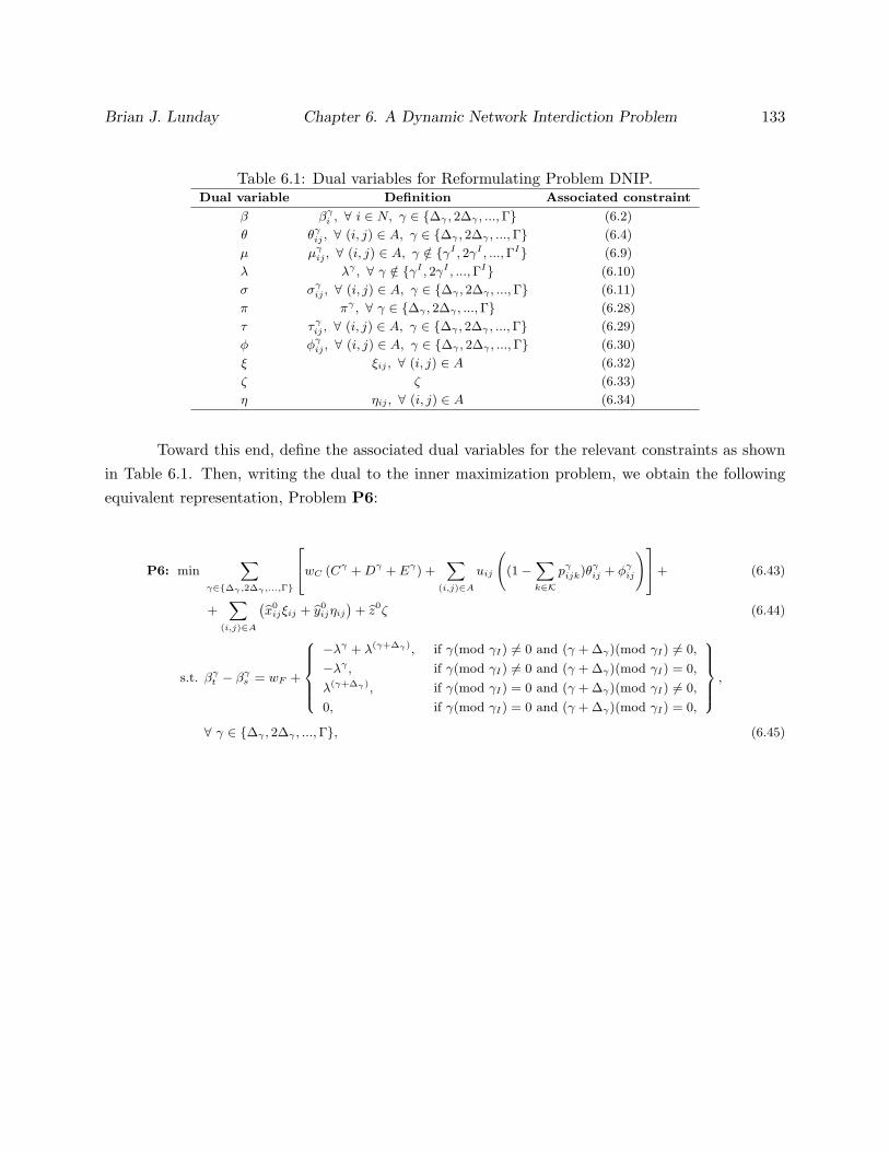
Brian J. Lunday Chapter 6. A Dynamic Network Interdiction Problem 133
Table 6.1: Dual variables for Reformulating Problem DNIP.Dual variable Definition Associated constraint
β βγi , ∀ i ∈ N, γ ∈ ∆γ , 2∆γ , ..., Γ (6.2)
θ θγij , ∀ (i, j) ∈ A, γ ∈ ∆γ , 2∆γ , ..., Γ (6.4)
µ µγij , ∀ (i, j) ∈ A, γ /∈ γI , 2γI , ..., ΓI (6.9)
λ λγ , ∀ γ /∈ γI , 2γI , ..., ΓI (6.10)
σ σγij , ∀ (i, j) ∈ A, γ ∈ ∆γ , 2∆γ , ..., Γ (6.11)
π πγ , ∀ γ ∈ ∆γ , 2∆γ , ..., Γ (6.28)
τ τγij , ∀ (i, j) ∈ A, γ ∈ ∆γ , 2∆γ , ..., Γ (6.29)
φ φγij , ∀ (i, j) ∈ A, γ ∈ ∆γ , 2∆γ , ..., Γ (6.30)
ξ ξij , ∀ (i, j) ∈ A (6.32)
ζ ζ (6.33)
η ηij , ∀ (i, j) ∈ A (6.34)
Toward this end, define the associated dual variables for the relevant constraints as shownin Table 6.1. Then, writing the dual to the inner maximization problem, we obtain the followingequivalent representation, Problem P6:
P6: min∑
γ∈∆γ ,2∆γ ,...,Γ
wC (Cγ + Dγ + Eγ) +∑
(i,j)∈A
uij
((1−
∑k∈K
pγijk)θγ
ij + φγij
)+ (6.43)
+∑
(i,j)∈A
(x0
ijξij + y0ijηij
)+ z0ζ (6.44)
s.t. βγt − βγ
s = wF +
−λγ + λ(γ+∆γ), if γ(mod γI) 6= 0 and (γ + ∆γ)(mod γI) 6= 0,
−λγ , if γ(mod γI) 6= 0 and (γ + ∆γ)(mod γI) = 0,
λ(γ+∆γ), if γ(mod γI) = 0 and (γ + ∆γ)(mod γI) 6= 0,
0, if γ(mod γI) = 0 and (γ + ∆γ)(mod γI) = 0,
,
∀ γ ∈ ∆γ , 2∆γ , ..., Γ, (6.45)

Brian J. Lunday Chapter 6. A Dynamic Network Interdiction Problem 134
βγi − βγ
j + θγij − τγ
ij ≥
−µγij + µ
(γ+∆γ)ij + σ
(γ+γE)ij , if
γ(mod γI) 6= 0
(γ + ∆γ)(mod γI) 6= 0
(γ + γE)(mod γE) = 0
,
−µγij + µ
(γ+∆γ)ij , if
γ(mod γI) 6= 0
(γ + ∆γ)(mod γI) 6= 0
(γ + γE)(mod γE) 6= 0
,
−µγij + σ
(γ+γE)ij , if
γ(mod γI) 6= 0
(γ + ∆γ)(mod γI) = 0
(γ + γE)(mod γE) = 0
,
−µγij , if
γ(mod γI) 6= 0
(γ + ∆γ)(mod γI) = 0
(γ + γE)(mod γE) 6= 0
,
µ(γ+∆γ)ij + σ
(γ+γE)ij , if
γ(mod γI) = 0
(γ + ∆γ)(mod γI) 6= 0
(γ + γE)(mod γE) = 0
,
µ(γ+∆γ)ij , if
γ(mod γI) = 0
(γ + ∆γ)(mod γI) 6= 0
(γ + γE)(mod γE) 6= 0
,
σ(γ+γE)ij , if
γ(mod γI) = 0
(γ + ∆γ)(mod γI) = 0
(γ + γE)(mod γE) = 0
,
0, if
γ(mod γI) = 0
(γ + ∆γ)(mod γI) = 0
(γ + γE)(mod γE) 6= 0
,
,
∀ (i, j) ∈ A, γ ∈ ∆γ , 2∆γ , ..., Γ, (6.46)
σγij + τγ
ij =
σ
(γ+∆γ)ij , if (γ + γE)(mod γE) 6= 0,
0, if (γ + γE)(mod γE) = 0,∀ (i, j) ∈ A, γ ∈ ∆γ , 2∆γ , ..., Γ, (6.47)
φγij − τγ
ij − gijπγ ≥ 0, ∀ (i, j) ∈ A, γ ∈ ∆γ , 2∆γ , ..., Γ, (6.48)
φγij + τγ
ij ≥ 0, ∀ (i, j) ∈ A, γ ∈ ∆γ , 2∆γ , ..., Γ, (6.49)
πγ = −wP , ∀ γ ∈ ∆γ , 2∆γ , ..., Γ, (6.50)
ξij = σγEij + µ
∆γ
ij , ∀ (i, j) ∈ A, (6.51)
ζ = λ∆γ , ∀ (i, j) ∈ A, (6.52)
ηij = σ∆γ
ij , ∀ (i, j) ∈ A, (6.53)
(θγij , φ
γij) ≥ 0, ∀ (i, j) ∈ A, k ∈ K, γ ∈ ∆γ , 2∆γ , ..., Γ,
Constraints (6.3), (6.5), (6.7)–(6.8), (6.12)–(6.27), (6.35)–(6.36),
pγijk ≥ 0, ∀ (i, j) ∈ A, k ∈ K, γ ∈ ∆γ , 2∆γ , ..., Γ.

Brian J. Lunday Chapter 6. A Dynamic Network Interdiction Problem 135
6.4 Illustration of Stability and Convergence Behavior
In this section, we consider two types of problem structures as embodied by two simple illustrativeexamples and examine the convergence of period-specific optimal strategies for three combinationsof interdictor and evader reaction times or decision cycle lengths, (γI , γE) ∈ (2, 2), (2, 3), (3, 2),and three time horizons, Γ ∈ 6, 12, 18. We examine Problem P6 for two instances with networktopology and parameters displayed in Figures 6.1(a) and 6.1(b), which have the following structuraldifference. Denote Z to be the number of distinct optimal solutions for deployment of the resourcesRk, ∀ k ∈ K, in the problem of minimizing the maximum flow through the network for a staticformulation. The instance in Figure 6.1(a) has Z = 1, and for such a case, we expect that, givensufficient budgetary resources and time periods, and a relatively small ratio wC/wF , the distinctstrategy that minimizes the maximum evader flow will be manifested as the stable equilibrium (i.e.,under such an outcome, the interdictor would not choose to incur costs related to the redeploymentof resources for the purposes of inflicting penalties upon the evader). On the other hand, forthe instance displayed in Figure 6.1(b), the interdiction costs have been modified to ensure thatalternative minimax flow solutions exist, thereby yielding Z > 1 and allowing for the possibility ofthe interdictor altering strategies between periods in order to inflict evader penalties, depending onthe respective weights (wC , wP ) and the related cost parameters.
s
1
2
t
1000
1000
100
12
11
1
s
s
s
c
c
u
200
1000
50
22
21
2
s
s
s
c
c
u
1000
200
50
21
11
1
t
t
t
c
c
u
1000
1000
100
22
12
2
t
t
t
c
c
u
K
K
K
kAjic
kAjic
kAjicd
Ajiug
AA
RR
BB
B
ww
ijkijk
ijkijk
ijkijk
ijij
PC
,),(,001.0
,),(,005.0
,),(,01.0
),(,1.0
01.0
02.0
50
/
,...,2,,1000
10
1,1,
21
21
21
3
s
1
2
t
1000
1000
100
12
11
1
s
s
s
c
c
u
200
200
50
22
21
2
s
s
s
c
c
u
200
200
50
21
11
1
t
t
t
c
c
u
1000
1000
100
22
12
2
t
t
t
c
c
u
(a) Instance with Z =1 (b) Instance with Z >1
Figure 6.1: Two Structurally Different DNIP Instances.
Note that the value ε = 10−3 as specified in Figure 6.1 is the parameter used for determiningwF via Proposition 6.1, whereas we employ a tighter relative optimality tolerance of 10−9 for solvingProblem P6 via the commercial solver BARON Version 8.1.5 (Ryoo and Sahinidis, 1996) using theGAMS modeling language on a 1.6 GHz Intel Pentium M processor running Linux. For our analysis,we assume that the interdictor begins with no available resources, and that the evader begins with

Brian J. Lunday Chapter 6. A Dynamic Network Interdiction Problem 136
the maximum uninterdicted flow through the network (z0, x0ij , ∀ (i, j) ∈ A), along with a consistent
perception thereof by way of setting y0ij = x0
ij , ∀ (i, j) ∈ A. We employed BARON with a timelimit of 360, 1800, and 3600 CPU seconds for the respective time horizons of Γ ∈ 6, 12, 18.
The derived value for wF varies for each instance in accordance with Proposition 6.1. Forall three cases of (γI , γE) ∈ (2, 2), (2, 3), (3, 2), we have ∆γ = 1, and the computation of wF byProposition 6.1 for both instances in Figure 6.1, given their identical uninterdicted upper boundson arc flows, uij , ∀ (i, j) ∈ A, results in wF = 1 + (1.5× 10⁷), 1 + (3.0× 10⁷), 1 + (4.5× 10⁷) forthe respective time horizons Γ ∈ 6, 12, 18.
Remark 6.2. In order to ensure the fidelity of the solver BARON, we scaled the objective func-tion in (6.1) to yield wF = 106 for each instance examined, with the parameters (wC , wP ) linearlyscaled accordingly. Without such scaling, the solver returned null solutions, wherein the interdictordid not procure or deploy any resources. Null solutions do represent a global optimal solution forcost-prohibitive instances of DNIP, wherein the procurement and/or deployment costs for resourcesexceed their interdiction benefit in (6.1), e.g., via empirical analysis, this occurs when wC > 108
for the instances presented in Figure 6.1 with Γ = 6. However, the parameters for the instancesin Figure 6.1 are not cost-prohibitive, and we further ensured the implausibility of null solutions(without scaling of the objective function) by setting wC ≡ 0 and running both instance structuresfor the different (Γ, γI , γE)-combinations. However, BARON still reported null solutions. There-fore, our proposed scaling of the objective function is necessary from the viewpoint of assuringBARON’s fidelity, and we apply this scaling technique for all the runs reported in the remainderof this section.
Note that for wP ≡ 0, Proposition 6.1 yields wF = 1 as a legitimate choice for any ε > 0.Accordingly, we tested the different (Γ, γI , γE)-combinations with (wC , wP , wF ) = (1, 0, 1), andverified that, in the absence of penalties inflicted upon the evader, the interdictor strategy indeedconverges to a minimax net flow solution and does not exhibit oscillation, while minimizing costsassociated with the redeployment of resources. This validates that the model reflects the intendedinterdictor and evader behaviors in the absence of evader penalties.
Examining the instance represented in Figure 6.1(a) for the case where neither the overallnor period-specific budgets represent active constraints in an optimal solution, the results wereconsistent across all (Γ, γI , γE)-combinations considered. In an optimal solution, the interdictorutilizes the maximum available amount of each resource type at the earliest opportunity (i.e.,Rγ+
k = Rk, for γ = γI , ∀ k ∈ K, and Rγ+k = 0 otherwise), and deploys them in a manner
to minimize the maximum flow for the remaining periods, resulting in pγ1t1 = pγ
s22 = 0.25 forγ ∈ γI , γI + ∆γ , γ
I + 2∆γ , ...,Γ, and pγijk = 0 otherwise. For several other instances of Problem
DNIP having a distinct optimal solution to minimize the maximum flow, and without budget

Brian J. Lunday Chapter 6. A Dynamic Network Interdiction Problem 137
limitations, we observed a similar attainment of a stable strategic equilibrium in a single decisioncycle.
In contrast to the foregoing single-cycle convergence to an equilibrium solution, the outcomewas quite different for the case of active budget constraints at optimality in the instance representedin Figure 6.1(a) (enforced by setting Bγ = 100, ∀ γ ∈ ∆γ , ...,Γ, where a single-period budgetequals the total cost to procure all available resources). For a particular representative instance hav-ing (Γ, γI , γE) = (6, 3, 2), Table 6.2 presents the optimal pγ
ijk-values, with dashed lines demarcatingthe interdictor’s decision cycles (with implied initial values of p0
ijk = 0, ∀ (i, j) ∈ A, k ∈ K). Theseresults exhibit two noteworthy characteristics. First, convergence to the same equilibrium strategiesas before is still attained, albeit at a later time period (γ = 6). Second, the interdictor procures lessthan the maximum available resources in period γI = 3, and then given these resources, allocatesthem in that same period to minimize the maximum evader flow. Within the context of the regretfunction (6.1) or (6.43), this is preferable to procuring all the resources Rk, ∀ k ∈ K, during periodγI = 3, but then not having any remaining capital to deploy any of these available resources untilthe next decision cycle, i.e., when γ = 2γI = 6.
Table 6.2: Optimal pγijk-values for the Instance of Figure 6.1(a) with (Γ, γI , γE) = (6, 3, 2) and
Bγ = 100, ∀ γ ∈ ∆γ , ...,Γ.γ pγ
s11 pγs21 pγ
1t1 pγ2t1 pγ
s12 pγs22 pγ
1t2 pγ2t2
1 0 0 0 0 0 0 0 0
2 0 0 0 0 0 0 0 0
3 0 0 0.2354 0 0 0.25 0 0
4 0 0 0.2354 0 0 0.25 0 0
5 0 0 0.2354 0 0 0.25 0 0
6 0 0 0.25 0 0 0.25 0 0
Next, consider the instance in Figure 6.1(b). The solver BARON terminated for all (γI , γE)-combinations due to the imposed computational time limits without attaining a global optimalsolution and, upon extending the computational time limit to 18000 CPU seconds (i.e., 5 CPUhours) for each instance, attained the relative % optimality gaps reported in Table 6.3. Althoughthese results indicate the inability of BARON to solve instances having longer time horizons, itis worth noting that the incumbent solution for each instance was identified by BARON withinthe first 1800 CPU seconds, with the remainder of the computational effort spent trying to verifyoptimality of this solution. Note also that, for each time horizon considered and given the samelimit on computational effort across (γI , γE)-combinations, the relative % optimality gap attainedis tigher for lower ratios of interdictor-to-evader cycle lengths (γI/γE), suggesting that an increasein the ratio of relative cycle lengths degrades solver performance.
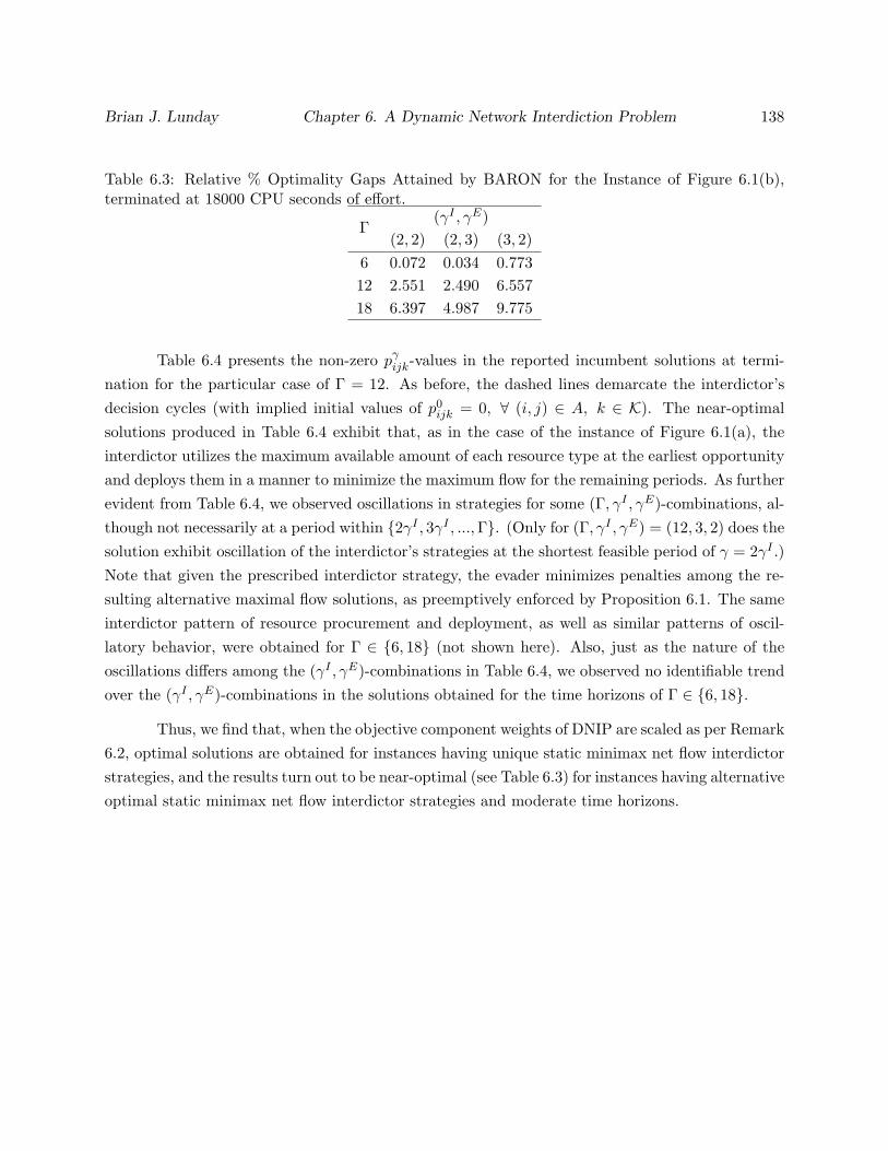
Brian J. Lunday Chapter 6. A Dynamic Network Interdiction Problem 138
Table 6.3: Relative % Optimality Gaps Attained by BARON for the Instance of Figure 6.1(b),terminated at 18000 CPU seconds of effort.
Γ(γI , γE)
(2, 2) (2, 3) (3, 2)6 0.072 0.034 0.77312 2.551 2.490 6.55718 6.397 4.987 9.775
Table 6.4 presents the non-zero pγijk-values in the reported incumbent solutions at termi-
nation for the particular case of Γ = 12. As before, the dashed lines demarcate the interdictor’sdecision cycles (with implied initial values of p0
ijk = 0, ∀ (i, j) ∈ A, k ∈ K). The near-optimalsolutions produced in Table 6.4 exhibit that, as in the case of the instance of Figure 6.1(a), theinterdictor utilizes the maximum available amount of each resource type at the earliest opportunityand deploys them in a manner to minimize the maximum flow for the remaining periods. As furtherevident from Table 6.4, we observed oscillations in strategies for some (Γ, γI , γE)-combinations, al-though not necessarily at a period within 2γI , 3γI , ...,Γ. (Only for (Γ, γI , γE) = (12, 3, 2) does thesolution exhibit oscillation of the interdictor’s strategies at the shortest feasible period of γ = 2γI .)Note that given the prescribed interdictor strategy, the evader minimizes penalties among the re-sulting alternative maximal flow solutions, as preemptively enforced by Proposition 6.1. The sameinterdictor pattern of resource procurement and deployment, as well as similar patterns of oscil-latory behavior, were obtained for Γ ∈ 6, 18 (not shown here). Also, just as the nature of theoscillations differs among the (γI , γE)-combinations in Table 6.4, we observed no identifiable trendover the (γI , γE)-combinations in the solutions obtained for the time horizons of Γ ∈ 6, 18.
Thus, we find that, when the objective component weights of DNIP are scaled as per Remark6.2, optimal solutions are obtained for instances having unique static minimax net flow interdictorstrategies, and the results turn out to be near-optimal (see Table 6.3) for instances having alternativeoptimal static minimax net flow interdictor strategies and moderate time horizons.
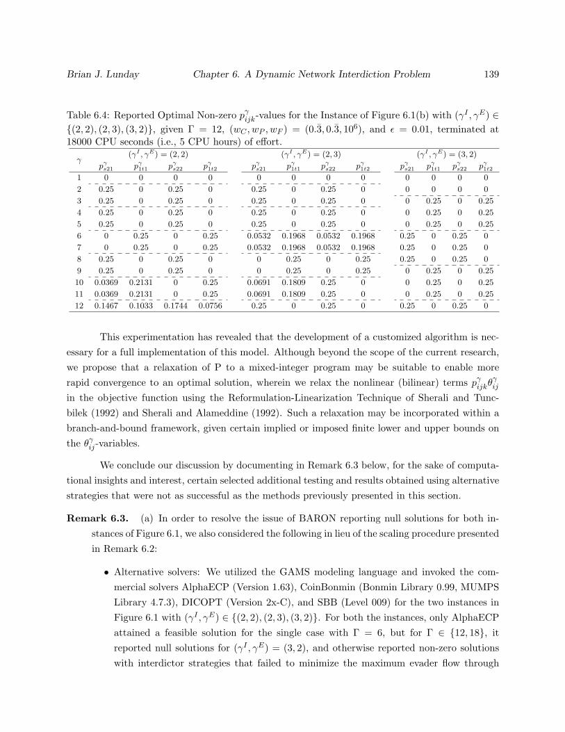
Brian J. Lunday Chapter 6. A Dynamic Network Interdiction Problem 139
Table 6.4: Reported Optimal Non-zero pγijk-values for the Instance of Figure 6.1(b) with (γI , γE) ∈
(2, 2), (2, 3), (3, 2), given Γ = 12, (wC , wP , wF ) = (0.3, 0.3, 106), and ε = 0.01, terminated at18000 CPU seconds (i.e., 5 CPU hours) of effort.
γ(γI , γE) = (2, 2) (γI , γE) = (2, 3) (γI , γE) = (3, 2)
pγs21 pγ
1t1 pγs22 pγ
1t2 pγs21 pγ
1t1 pγs22 pγ
1t2 pγs21 pγ
1t1 pγs22 pγ
1t2
1 0 0 0 0 0 0 0 0 0 0 0 0
2 0.25 0 0.25 0 0.25 0 0.25 0 0 0 0 0
3 0.25 0 0.25 0 0.25 0 0.25 0 0 0.25 0 0.25
4 0.25 0 0.25 0 0.25 0 0.25 0 0 0.25 0 0.25
5 0.25 0 0.25 0 0.25 0 0.25 0 0 0.25 0 0.25
6 0 0.25 0 0.25 0.0532 0.1968 0.0532 0.1968 0.25 0 0.25 0
7 0 0.25 0 0.25 0.0532 0.1968 0.0532 0.1968 0.25 0 0.25 0
8 0.25 0 0.25 0 0 0.25 0 0.25 0.25 0 0.25 0
9 0.25 0 0.25 0 0 0.25 0 0.25 0 0.25 0 0.25
10 0.0369 0.2131 0 0.25 0.0691 0.1809 0.25 0 0 0.25 0 0.25
11 0.0369 0.2131 0 0.25 0.0691 0.1809 0.25 0 0 0.25 0 0.25
12 0.1467 0.1033 0.1744 0.0756 0.25 0 0.25 0 0.25 0 0.25 0
This experimentation has revealed that the development of a customized algorithm is nec-essary for a full implementation of this model. Although beyond the scope of the current research,we propose that a relaxation of P to a mixed-integer program may be suitable to enable morerapid convergence to an optimal solution, wherein we relax the nonlinear (bilinear) terms pγ
ijkθγij
in the objective function using the Reformulation-Linearization Technique of Sherali and Tunc-bilek (1992) and Sherali and Alameddine (1992). Such a relaxation may be incorporated within abranch-and-bound framework, given certain implied or imposed finite lower and upper bounds onthe θγ
ij-variables.
We conclude our discussion by documenting in Remark 6.3 below, for the sake of computa-tional insights and interest, certain selected additional testing and results obtained using alternativestrategies that were not as successful as the methods previously presented in this section.
Remark 6.3. (a) In order to resolve the issue of BARON reporting null solutions for both in-stances of Figure 6.1, we also considered the following in lieu of the scaling procedure presentedin Remark 6.2:
• Alternative solvers: We utilized the GAMS modeling language and invoked the com-mercial solvers AlphaECP (Version 1.63), CoinBonmin (Bonmin Library 0.99, MUMPSLibrary 4.7.3), DICOPT (Version 2x-C), and SBB (Level 009) for the two instances inFigure 6.1 with (γI , γE) ∈ (2, 2), (2, 3), (3, 2). For both the instances, only AlphaECPattained a feasible solution for the single case with Γ = 6, but for Γ ∈ 12, 18, itreported null solutions for (γI , γE) = (3, 2), and otherwise reported non-zero solutionswith interdictor strategies that failed to minimize the maximum evader flow through

Brian J. Lunday Chapter 6. A Dynamic Network Interdiction Problem 140
the network, as attained in the solutions reported by BARON. Moreover, we also im-plemented AlphaECP for the special case of wC = 0, but its reported solutions did notimprove with respect to optimization of flow, further evidencing its ineffectiveness insolving DNIP instances.
• Alternative scaling magnitudes for wF : In deciding to scale the objective function in (6.1)as per Remark 6.2, we also considered scaled values of wF ∈ 107, 105, 104, 103. WhilewF = 107 yielded null solutions, the scaled values of wF ∈ 105, 104, 103 provided non-null solutions. However, the implemented scaling technique such that wF = 106 (whichinduces wC = wP = 0.06 for Γ = 18), not only yields non-null optimal solutions but alsoreduces the possibility of further fidelity issues due to more significant reductions in theother objective function components.
(b) To improve the performance of BARON for the instance of Figure 6.1(b), we also attemptedthe following:
• Scaling and rounding of weights in (6.1): We implemented BARON after scaling (6.1)to yield wF = 106, and then rounding up the other scaled weights to (at least) wC = 1and wP = 1. Although this scaling-and-rounding technique did improve solution qualityfor 67% of the instances examined, with BARON still terminating due to time limitconstraints, it reported null solutions for all instances with (γI , γE) = (3, 2), renderingit inappropriate as a general approach.
• Examining model behavior with wC ≡ 0: Since the software BARON terminated dueto time constraints, we conducted additional testing on the instance in Figure 6.1(b)with wC ≡ 0 in order to examine the efficacy of BARON in solving DNIP instances. Inan optimal solution for such a cost-neutral case where neither the overall nor period-specific budgets represent active constraints in an optimal solution, the interdictor willpreemptively minimize the maximum evader flow, and maximize the minimum subse-quent evader penalties among the resulting alternative maximal flow solutions, i.e., theinterdictor should completely procure each resource at γ = γI and immediately allocateeach, in total, to either arc (s, 2) or (1, t), and subsequently reallocate each (in total)between the two arcs every γI periods. As in the case of wC = 1, BARON again termi-nated for all instances without attaining a global optimal solution due to our imposedcomputational time limits, reporting near-optimal solutions that minimize the maximumflow for all periods γ ≥ γI = 2 (as preemptively imposed by Proposition 6.1), but whichdo not maximize the minimum subsequent evader penalties among the resulting alterna-tive optimal maximal flow solutions. This indicates that it is the consideration of evaderpenalties in (6.1) that is problematic for BARON in attaining global optimal solutionswhen wC ≡ 0, and suggests that the same cause of having 0 < wP wF may be the

Brian J. Lunday Chapter 6. A Dynamic Network Interdiction Problem 141
principal source of difficulty with BARON when wC > 0.
• Resequencing of bilinear terms and constraints: We considered the formulation for Prob-lem P6 with objective function weights scaled as per Remark 6.2, but also with thebilinear terms pγ
ijkθγij in the objective function (6.43) transposed in the GAMS represen-
tation of the model representation in order to allow for possible variations in BARON’sperformance due to the sequencing of polynomial terms. In addition, we arranged theconstraints involving binary decision variables (i.e., Constraints (6.14)–(6.16), (6.21)–(6.23)) before all other constraints in the GAMS model representation, in order to enableBARON to potentially affect a more efficient variable fixing and branching process. Noidentifiable improvement in solution quality resulted from this experiment.
6.5 Conclusions and Recommendations.
In this chapter, we have proposed and formulated a novel multi-objective dynamic network interdic-tion problem, and have developed a solution procedure for which the commercial software BARON(Version 8.1.5) attains optimal or, for moderate time horizons, near-optimal solutions, dependingon the presence of alternative optimal static strategies that minimize the maximum evader flow.We have also investigated certain stability/oscillatory issues predicated on the latter structuralproperty using two representative problem instances.
For future study, we propose that our model be modified to account for interdictor costsusing goal programming. For government bureaucratic agencies that act as an interdictor, budgetsare often soft constraints. Agencies do underspend and overspend their budgets, both in fiscalquarters and fiscal years. They are penalized for overspending (hopefully), but there is also anassociated penalty for underspending a budget, as funds may be diverted to other competingbudget-deficit agencies. Conceptually, a combination of these factors implies the possibility thatoverspending may incur a net gain up to a certain threshold, and a penalty beyond it. Therefore, anextended model might consider a fourth component in the weighted objective function: a penaltycost for variations in expenditures from authorized budget levels. Typically, this would be weightedmuch lower than the terms pertaining to the interdiction being performed, but this would dependon the severity of the interdiction scenario and the overall fiscal state of the interdictor’s budgetaryresources. Furthermore, we suggest the expansion of the model formulation to account for arc-wisesuperadditive synergy between resources, whether in linear, convex, or general nonlinear forms,as examined by Lunday and Sherali (2009b). Finally, we propose the development of customizedalgorithms to solve the dynamic network interdiction problem, wherein a suitable relaxation isdesigned and embedded within a branch-and-bound framework.
Chapter 7
Equitable Apportionment of Railcars
within a Pooling Agreement for
Shipping Automobiles
7.1 Introduction
In this chapter, we present our research on the capital allocation problem, as introduced in Sec-tion 1.1.5. To recall the organization within this chapter, as outlined in Section 7.2, we presentour notation and detail the current fleet sizing and railcar allocation methods. In Section 7.3, wedemonstrate the effect of graph connectivity on equity in the current industrial practice, and ac-cordingly advocate instance disaggregation when the underlying network has multiple components.In Section 7.4, we illustrate another shortcoming of the present allocation scheme and propose foureffective alternative shipper allocation schemes. Likewise, in Section 7.5, we provide insights intothe existing carrier allocation scheme and design an alternative methodology. In Section 7.6, wecompute and compare shipper and carrier allocations for realistic test problems using combinationsof both current and proposed techniques, and we conclude the study in Section 7.7 with a summaryalong with recommendations for implementation and for future research.
142

Brian J. Lunday Chapter 7. Railcar Apportionment Problem 143
7.2 Fleet Sizing and Present Allocation Scheme Used in the In-
dustry
In this section, we present the relevant model, notation, and current static and dynamic fleet sizingprocesses used in the U.S. rail industry for shipping automobiles, followed by an overview andillustration of the present allocation scheme for shippers and carriers.
7.2.1 Model, Notation and Fleet Sizing Process
Consider the following fleet sizing process, which is performed for each of six equipment types asdescribed by Sherali and Maguire (2000). We will focus on any such equipment type, and assumethat it involves the shipment of automobiles for a group of manufacturers or shippers k = 1, ...,K,by a collection of r = 1, ..., R railroads or carriers participating in a pooling agreement.
Suppose that we are given the following data:
• k ∈ K ≡ 1, ...,K: index set of shippers.
• r ∈ R ≡ 1, ..., R: index set of railroads involved in performing loaded movements.
• i ∈ I ≡ 1, ...,m: index set of origin nodes for shipping automobiles.
• j ∈ J ≡ 1, ..., n: index set of destination nodes for shipping automobiles.
• k(i): shipper associated with origin node i, for i ∈ I.
• Ok = i ∈ I : k(i) = k, i.e., shipper k is associated with this origin node i, for k ∈ K.
• OD: set of origin-destination (O-D) pairs (i, j) for loaded movements.
• ODk: (i, j) ∈ OD : O-D pair (i, j) is associated with shipper k , for k ∈ K.
• Qij : daily loaded flow (railcars) for (i, j) ∈ OD.
• tij : loaded transit time (days) for (i, j) ∈ OD.
• tqij = queue time (defined as the days in advance that railcars must be made available for thesake of preparation) specified for O-D pair (i, j) ∈ OD.
• β = bad-order factor that reflects delays due to railcar maintenance and repair. This factor iscomputed separately for each equipment type, and has historically ranged as high as 1.12 (fortrilevels, when the a high demand for sport utility vehicles in the automobile market increased
Brian J. Lunday Chapter 7. Railcar Apportionment Problem 144
the relative demand for trilevel carriers), although representative bad-order factors in thecurrent market are approximately 1.02 and 1.03 for bilevel and trilevel railcars, respectively.
• k(i, j): shipper associated with O-D pair (i, j) ∈ OD.
• fLijr: fraction of loaded railcar-days on O-D pair (i, j) that is associated with railroad r, ∀ (i, j) ∈OD, r ∈ R. (Note that
∑r∈R
fLijr = 1, ∀ (i, j) ∈ OD.)
• A: set of empty return routes (p, q) from unloading ramp p to loading location q.
• fEpqr : fraction of the empty return route (p, q) for which railroad r is responsible with respect
to moving the railcars, ∀ (p, q) ∈ A, r ∈ R . (Note that∑r∈R
fEpqr ≤ 1, ∀ (p, q) ∈ A, because
there might be other extraneous railroads that assist in moving the empty railcars, wheresuch railroads are compensated separately by the shippers.)
• τpq: transit time (days) on the empty return route (p, q) ∈ A.
Now, suppose that we run the static and the dynamic fleet sizing models as described inSherali and Tuncbilek (1997) and in Sherali and Maguire (2000). Let the following information bederived from these model runs.
• (xpq, ∀ (p, q) ∈ A): flow solution (railcars) obtained for the empty railcar repositioningtransportation problem in the static model run.
• Fs: fleet size (railcars) determined by the static model run. Note that from Sherali andTuncbilek (1997), Fs equals the total loaded plus empty railcar-days (on a daily basis), i.e.,we have,
Fs ≡∑∑(i,j)∈OD
tijQij +∑∑(p,q)∈A
τpqxpq. (7.1)
• φi: weighted average empty return time (days) to origin i, computed as the sum of the emptyrailcar-days on the return flow to origin i divided by the total return flow into origin i. Hence,
φi =
∑p:(p,i)∈A
τpixpi∑p:(p,i)∈A
xpi
, (7.2)
where note that, ∑p:(p,i)∈A
xpi =∑
j:(i,j)∈OD
Qij , ∀ i ∈ I. (7.3)

Brian J. Lunday Chapter 7. Railcar Apportionment Problem 145
• Fd: fleet size (railcars) determined by the dynamic model run (considering demand fluctua-tions over time).
• DF : dynamic factor computed as DF ≡ Fd/Fs. Historically, these factors range from 1.1 to1.3.
• Fs(i,j): fleet size component of Fs that is allocated to O-D pair (i, j) according to
Fs(i,j) ≡ Qij(tij + φi), ∀ (i, j) ∈ OD. (7.4)
Note that from (7.1)–(7.4), we have,∑∑(i,j)∈OD
Fs(i,j) =∑∑(i,j)∈OD
tijQij +∑
i
φi
∑j:(i,j)∈OD
Qij
=∑∑(i,j)∈OD
tijQij +∑
i
∑p:(p,i)∈A
τpixpi ≡ Fs. (7.5)
Next, let
• F as(i,j): adjusted fleet size for each O-D pair (i, j) ∈ OD based on queue times and the
bad-order factor, where from (7.4),
F as(i,j) ≡ Fs(i,j)
[1 +
tqij(tij + φi)
]β = Qij
(tij + φi + tqij
)β. (7.6)
• FAF k: forecast accuracy factor for shipper k ∈ K, computed over a three-year average as inSherali and Maguire (2000) to reflect the historical estimate of the ratio of actual to forecastedannual railcar loads shipped. (Although the TTX Reload Group has examined the possibilityof utilizing arc-specific forecast accuracy factors for each shipper, i.e., FAFk(i,j), ∀ (i, j) ∈OD, k ∈ K, in order to improve the model resolution, no such measure has been adopted todate; nonetheless, such arc-specific factors can be readily accommodated within the analysisbelow.)
• FS(i, j): Total fleet size attributed to O-D pair (i, j), where,
FS(i, j) = F as(i,j)(DF )− F a
s(i,j)
(1− FAF k(i)
), ∀ (i, j) ∈ OD. (7.7)
We remark here that although (7.7) is the formula used in practice based on negotiations betweenshippers and carriers, since the corrections due to the dynamic factor and the forecast accuracy
Brian J. Lunday Chapter 7. Railcar Apportionment Problem 146
factor are multiplicative, we could alternatively have computed
FS(i, j) = F as(i,j)(DF )(FAF k(i)), ∀ (i, j) ∈ OD. (7.8)
Note that (7.7) and (7.8) coincide if either DF = 1 or FAF k(i) = 1, i.e., under no (or sufficientlylow) day-to-day variations in loaded flows, or under accurate historical forecasts.
In either case, the total prescribed fleet size is computed as
FS =∑∑(i,j)∈OD
FS(i, j). (7.9)
7.2.2 Present Allocation Scheme Used in the Industry
Presently, a two-step procedure is adopted to determine fleet size allocations. The first step belowdetermines allocations made to individual shippers, and the second step then determines the railroadallocations.
Present Allocation Scheme (PAS):
Step 1. (Shipper Allocations): Let FS(i, j) be given by (7.7). Then, the total fleet sizeallocated to shipper k under PAS is given by
FSPAS(k) =∑∑
(i,j)∈ODk
FS(i, j). (7.10)
Step 2. (Railroad Allocations): Let Lrk be the total loaded railcar-days of business thatrailroad r conducts for shipper k. This quantity can be computed as
Lrk =∑∑
(i,j)∈ODk
fLijrQijtij , ∀ r ∈ R k ∈ K. (7.11)
Note that ∑r∈R
Lrk ≡∑∑
(i,j)∈ODk
Qijtij (7.12)
represents the total loaded railcar-days of shipment corresponding to shipper k ∈ K.
Then, define the following:
• FSPASrk : allocation of shipper k’s allotment FSPAS(k) that is made to railroad r under PAS;
• FSPASr : allocation of railcars made to railroad r under PAS.

Brian J. Lunday Chapter 7. Railcar Apportionment Problem 147
Thus, we have
FSPASrk ≡ FSPAS(k)
Lrk∑ρ∈R
Lρk
, ∀ r ∈ R, k ∈ K, (7.13)
FSPASr =
∑k∈K
FSPASrk , ∀ r ∈ R. (7.14)
Note that the allocation (7.13) distributes shipper k’s allotment FSPAS(k) to the railroads inproportion to the total loaded railcar-days of business they conduct with it.
Example 7.1. Consider a situation in which we have K = 2 shippers and R = 2 railroads,and where the rail network has two origin nodes (nodes 1 and 2), and two destination nodes(nodes 3 and 4). The specific data in terms of the foregoing notation is listed in Table 7.1, basedon a network topology of OD = (1, 3), (1, 4), and (2, 4) and A = (3, 1), (3, 2), (4, 1), (4, 2),wherein OD1 = (1, 3) and (1, 4) with O1 = 1, and OD2 = (2, 4) with O2 = 2. (Hence,k(1, 3) = k(1, 4) = k(1) = 1, and k(2, 4) = k(2) = 2.)
Table 7.1: Instance Data for Example 7.1.(i, j) (1, 3) (1, 4) (2, 3) (2, 4)Qij 15 10 – 12tij 1 2 – 1
(fLij1, f
Lij2) (1,0) (0,1) (–,–) (0.5,0.5)
τji 1 2 1 2(fE
ji1, fEji2) (1,0) (0,1) (1,0) (0.5,0.5)
For simplicity in illustration, let us assume that
tqij = 0, ∀ (i, j) ∈ OD;β = 1;DF = 1; and FAF k = 1, ∀ k ∈ K. (7.15)
Given this data, the empty railcar repositioning transportation problem (see Sherali and Tuncbilek,1997) and an optimal solution are as displayed in Figure 7.1. Note that from Figure 7.1(b), wehave
x31 = 15, x32 = 0, x41 = 10, and x42 = 12. (7.16)
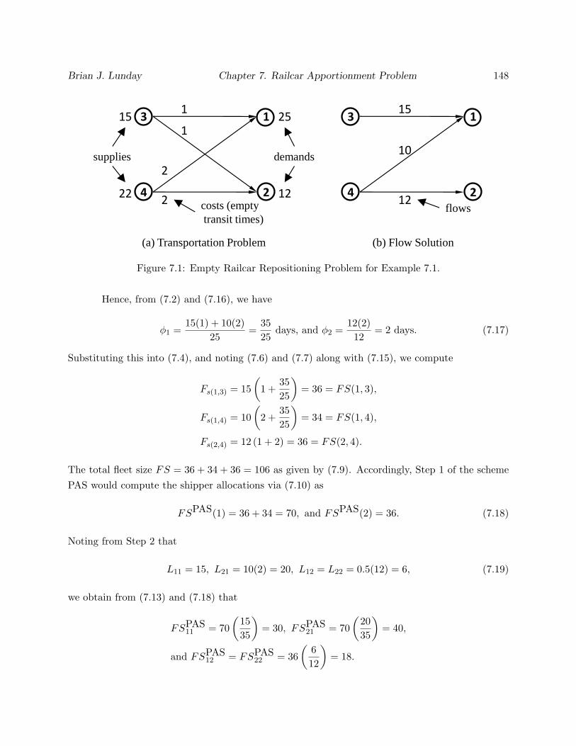
Brian J. Lunday Chapter 7. Railcar Apportionment Problem 148
3
4
1 25
2 12
15
22
1
1
2
2
supplies demands
costs (empty
transit times)
(a) Transportation Problem (b) Flow Solution
3
4
1
2
15
10
12flows
Figure 7.1: Empty Railcar Repositioning Problem for Example 7.1.
Hence, from (7.2) and (7.16), we have
φ1 =15(1) + 10(2)
25=
3525
days, and φ2 =12(2)12
= 2 days. (7.17)
Substituting this into (7.4), and noting (7.6) and (7.7) along with (7.15), we compute
Fs(1,3) = 15(
1 +3525
)= 36 = FS(1, 3),
Fs(1,4) = 10(
2 +3525
)= 34 = FS(1, 4),
Fs(2,4) = 12 (1 + 2) = 36 = FS(2, 4).
The total fleet size FS = 36 + 34 + 36 = 106 as given by (7.9). Accordingly, Step 1 of the schemePAS would compute the shipper allocations via (7.10) as
FSPAS(1) = 36 + 34 = 70, and FSPAS(2) = 36. (7.18)
Noting from Step 2 that
L11 = 15, L21 = 10(2) = 20, L12 = L22 = 0.5(12) = 6, (7.19)
we obtain from (7.13) and (7.18) that
FSPAS11 = 70
(1535
)= 30, FSPAS
21 = 70(
2035
)= 40,
and FSPAS12 = FSPAS
22 = 36(
612
)= 18.
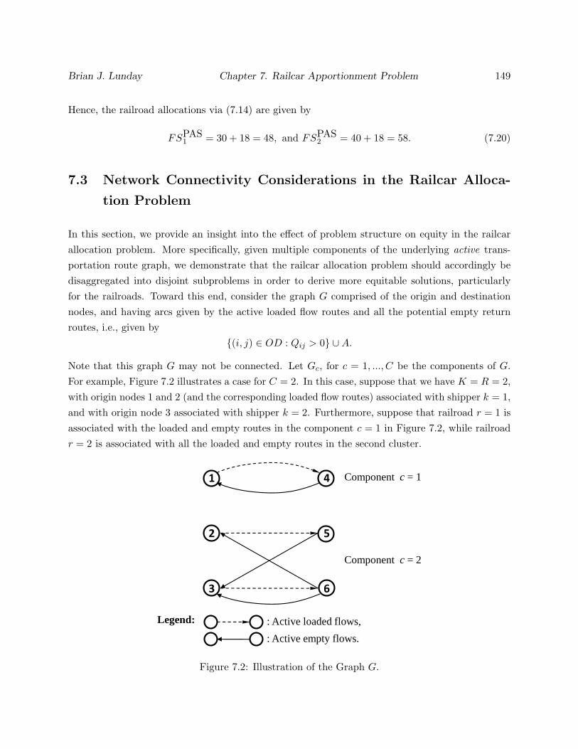
Brian J. Lunday Chapter 7. Railcar Apportionment Problem 149
Hence, the railroad allocations via (7.14) are given by
FSPAS1 = 30 + 18 = 48, and FSPAS
2 = 40 + 18 = 58. (7.20)
7.3 Network Connectivity Considerations in the Railcar Alloca-
tion Problem
In this section, we provide an insight into the effect of problem structure on equity in the railcarallocation problem. More specifically, given multiple components of the underlying active trans-portation route graph, we demonstrate that the railcar allocation problem should accordingly bedisaggregated into disjoint subproblems in order to derive more equitable solutions, particularlyfor the railroads. Toward this end, consider the graph G comprised of the origin and destinationnodes, and having arcs given by the active loaded flow routes and all the potential empty returnroutes, i.e., given by
(i, j) ∈ OD : Qij > 0 ∪A.
Note that this graph G may not be connected. Let Gc, for c = 1, ..., C be the components of G.For example, Figure 7.2 illustrates a case for C = 2. In this case, suppose that we have K = R = 2,with origin nodes 1 and 2 (and the corresponding loaded flow routes) associated with shipper k = 1,and with origin node 3 associated with shipper k = 2. Furthermore, suppose that railroad r = 1 isassociated with the loaded and empty routes in the component c = 1 in Figure 7.2, while railroadr = 2 is associated with all the loaded and empty routes in the second cluster.
2
3
5
6
Component c = 11 4
Component c = 2
Legend: : Active loaded flows,
: Active empty flows.
Figure 7.2: Illustration of the Graph G.

Brian J. Lunday Chapter 7. Railcar Apportionment Problem 150
In addition, assume that the computations leading to Equation (7.7) yield
FS(1, 4) = 10, FS(2, 5) = 20, and FS(3, 6) = 10. (7.21)
Hence, from (7.10), we have that FSPAS(1) = 30 and FSPAS(2) = 10. Now, if L11 = L21 = 5,L12 = 0, and L22 = 5, then (7.13) and (7.14) would yield
FSPAS11 = 30
(510
)= 15, FSPAS
21 = 30(
510
)= 15, FSPAS
12 = 0, and
FSPAS22 = 10, with FSPAS
1 = 15 and FSPAS2 = 25.
(7.22)
However, noting the railroads associated with each cluster, we would logically expect the fleet allo-cation to railroads 1 and 2 to coincide with the fleet sizes associated respectively with components1 and 2 of G, namely, 10 railcars and 30 railcars via the respective (7.21), and not as given by(7.22).
The point here is that the active loaded and empty railcar flow networks are separate foreach component, and as such, the performance and requirements related to any one component inno way influences any other component. Hence, for prescribing equitable railcar allocations, eachcomponent of G must be treated separately. In essence, this is similar to the separable considerationof different equipment types in both the fleet sizing and railcar allocation processes. Therefore, wewill henceforth assume that the entire fleet size computation and allocation analysis is conductedseparately for each equipment type and for each component of the corresponding graph G.
7.4 Alternative Approaches for Shipper Allocations
In this section, we describe four techniques to allocate a dynamically-sized fleet of empty railcarsto shippers, based respectively on transit plus queuing time consideration within a total loadedrailcar-days proportionality factor; two techniques that utilize a marginal cost analysis to assessthe effect of individual shippers on the overall railcar requirement; and a game-theoretic Shapley-value approach, all of which portend improved equity among shippers with respect to the currentindustry standard. Notationally, we denote FSSAα(k) to be the total fleet size allocated undershipper allocation scheme α (i.e., under SAα) to shipper k, for all α = 1, 2, 3, 4, k ∈ K.

Brian J. Lunday Chapter 7. Railcar Apportionment Problem 151
7.4.1 Deficiencies of the Present Allocation Scheme and a Transit Plus Queuing
Time-based Scheme
We first provide an insight that motivates a modification of the present allocation scheme, basedon the manner in which the fleet size is allocated to each shipper via Equation (7.10). Note thatEquation (7.10) assigns to each shipper k the total fleet size allocated to its corresponding O-D pairs(i, j). Each of the latter values, FS(i, j), depends via (7.4)–(7.8) on the quantity φi, in particular,which by (7.2) is a weighted average estimate of the empty return time to the corresponding origin i.However, the entire purpose of the pooling agreement is to consolidate resources in order to derivea greatest overall efficiency. In achieving this goal, certain sections of the transportation networkmight incur greater empty transit costs than other portions, depending on the compromise madeby the solution process in repositioning the empty railcars at a minimal total cost. Hence, shippersassociated with origin nodes to which relatively quicker return routes are active in the empty railcarrepositioning solution x will stand to benefit over other shippers by way of being allotted a relativelysmaller fleet size component. In fact, as illustrated in Example 7.2 below, alternative optimalempty railcar repositioning solutions can lead to different fleet allocations. This is undesirablebecause different participants would prefer different alternative solutions, all of which are equallyadmissible by the pooling agreement operational guidelines. Hence, a conflicting situation arises.
In the modified scheme SA1, we propose the following simpler method. Let FS be thetotal fleet size determined as in (7.9). Let L(k) be the total loaded railcar-days including the queuetimes associated with shipper k, i.e.,
L(k) =∑∑
(i,j)∈ODk
Qij(tij + tqij), ∀ k ∈ K. (7.23)
Then, under the modified scheme SA1, we allocate to each shipper k the fraction of FS that isin direct proportion to its total loaded railcar-days of business on the network (including queuetimes), i.e.,
FSSA1(k) = FS
L(k)∑k′∈K
L(k′)
, ∀ k ∈ K. (7.24)
To see the relationship between PAS and SA1, let us define φ′i as an alternative value to φi
Brian J. Lunday Chapter 7. Railcar Apportionment Problem 152
of Equation (7.2), which attributes an empty return time to node i according to:
φ′i ≡ ν
∑
j:(i,j)∈OD
Qij(tij + tqij)∑∑(i,j)∈OD
Qij(tij + tqij)
1∑j:(i,j)∈OD
Qij
, ∀ i ∈ I, (7.25)
where ν is the total empty railcar-days given by
ν =∑∑(p,q)∈A
τpqxpq. (7.26)
Note that φ′i assigns a fraction of the total empty railcar days ν to node i in proportion to the loadedrailcar-days (including queue times) associated with the O-D arcs having node i as the origin, anddivides this fraction by the total loaded flow emanating from node i (which equals the total emptyflow coming into node i by Equation (7.3)), to derive an empty return time allocation. Observe thatthis allocation now considers the overall efficiency of the empty repositioning problem as reflectedby ν, unlike φi determined by (7.2), which considers only the local attribute of empty railcar-daysassociated with node i.
The following result provides a further insight that, under the condition of uniform forecastaccuracy factors, if we were to use φ′i in lieu of φi, ∀ i, in the scheme PAS of the foregoing section,then the total fleet size would remain invariant, and moreover, the fleet allocation via (7.2) wouldmatch that via the modified scheme (7.24).
Proposition 7.1. Assume that the forecast accuracy factor FAFk ≡ FAF, ∀ k ∈ K. Let φi andφ′i be defined via (7.2) and (7.25), respectively, for each i ∈ I. Suppose that we apply PAS whileusing φ′i in lieu of φi to determine the fleet size FS′ via (7.4)–(7.7) and (7.9), and to determinethe allocation FSPAS′(k) for each k ∈ K via (7.10). Then, we have,
FS′ = FS, (7.27a)
and FSPAS′(k) = FSSA1(k), ∀ k ∈ K. (7.27b)
Proof. Note that from Equations (7.6), (7.7), and (7.9), the fleet size FS′ determined using φ′i inlieu of φi is given by
FS′ = β (DF − 1 + FAF )∑∑(i,j)∈OD
Qij
(tij + φ′i + tqij
). (7.28)
Brian J. Lunday Chapter 7. Railcar Apportionment Problem 153
Using (7.25), we obtain
∑∑(i,j)∈OD
Qijφ′i =
∑i∈I
φ′i
∑j:(i,j)∈OD
Qij
= ν
∑∑(i,j)∈OD
Qij(tij + tqij)∑∑(i,j)∈OD
Qij(tij + tqij)
= ν. (7.29)
Likewise, from (7.2), (7.3) and (7.26), we obtain
∑∑(i,j)∈OD
Qijφi =∑i∈I
φi
∑j:(i,j)∈OD
Qij
=∑i∈I
φi
∑p:(p,i)∈A
xpi =∑i∈I
∑p:(p,i)∈A
τpixpi = ν. (7.30)
Examining (7.28) along with (7.29) and (7.30), it follows that the total fleet size given by (7.28)remains invariant whether we use φ′i or φi, ∀ i, in this formula, which establishes (7.27a).
Next, consider Equation (7.27b). For any k ∈ K, from (7.10), using (7.6) and (7.7) with φi
replaced by φ′i, ∀ i, we have,
FSPAS′(k) = β (DF − 1 + FAF )∑∑
(i,j)∈ODk
Qij(tij + φ′i + tqij). (7.31)
Furthermore, from (7.24), using (7.23) and (7.9), we have
FSSA1(k) = β (DF − 1 + FAF )∑∑(i,j)∈OD
Qij(tij + φ′i + tqij)
∑∑
(i,j)∈ODk
Qij(tij + tqij)∑∑(i,j)∈OD
Qij(tij + tqij)
.Using (7.29) in this equation results in
FSSA1(k) = β (DF − 1 + FAF )∑∑
(i,j)∈ODk
Qij(tij + tqij)
1 +ν∑∑
(i,j)∈OD
Qij(tij + tqij)
. (7.32)
But from (7.25), we obtain ν∑∑(i,j)∈OD
Qij(tij + tqij)
∑j:(i,j)∈OD
Qij(tij + tqij) =∑
j:(i,j)∈OD
Qijφ′i.
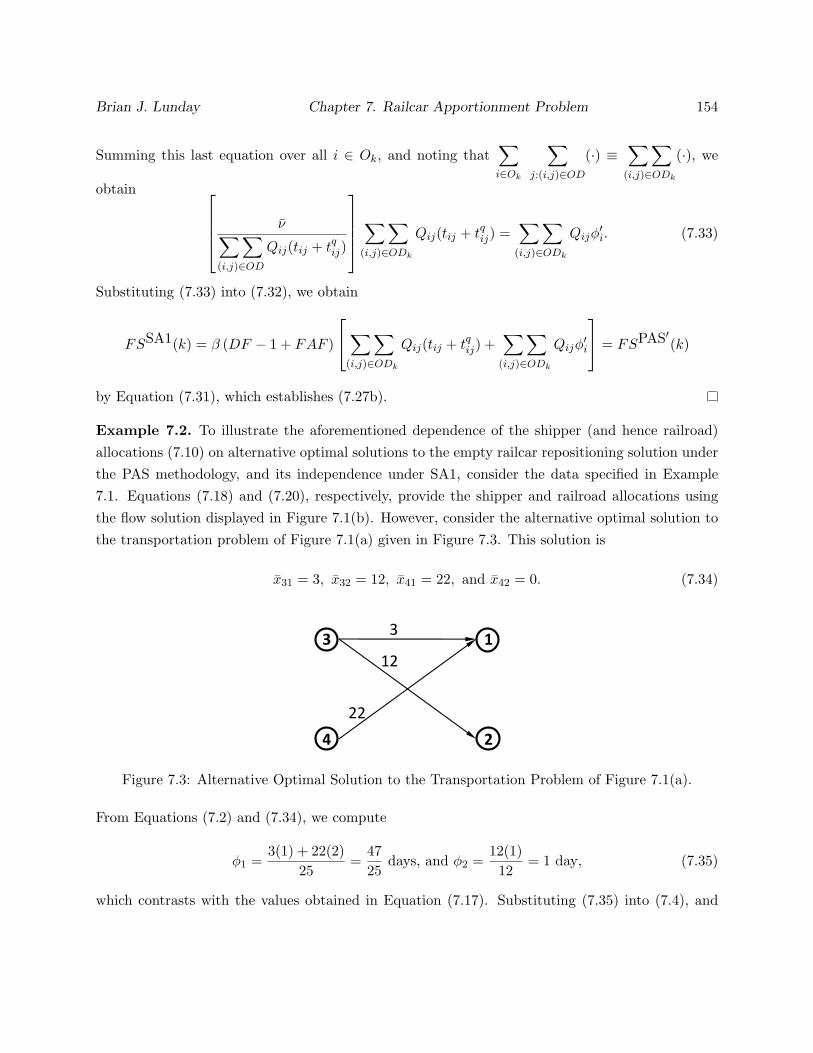
Brian J. Lunday Chapter 7. Railcar Apportionment Problem 154
Summing this last equation over all i ∈ Ok, and noting that∑i∈Ok
∑j:(i,j)∈OD
(·) ≡∑∑
(i,j)∈ODk
(·), we
obtain ν∑∑(i,j)∈OD
Qij(tij + tqij)
∑∑(i,j)∈ODk
Qij(tij + tqij) =∑∑
(i,j)∈ODk
Qijφ′i. (7.33)
Substituting (7.33) into (7.32), we obtain
FSSA1(k) = β (DF − 1 + FAF )
∑∑(i,j)∈ODk
Qij(tij + tqij) +∑∑
(i,j)∈ODk
Qijφ′i
= FSPAS′(k)
by Equation (7.31), which establishes (7.27b).
Example 7.2. To illustrate the aforementioned dependence of the shipper (and hence railroad)allocations (7.10) on alternative optimal solutions to the empty railcar repositioning solution underthe PAS methodology, and its independence under SA1, consider the data specified in Example7.1. Equations (7.18) and (7.20), respectively, provide the shipper and railroad allocations usingthe flow solution displayed in Figure 7.1(b). However, consider the alternative optimal solution tothe transportation problem of Figure 7.1(a) given in Figure 7.3. This solution is
x31 = 3, x32 = 12, x41 = 22, and x42 = 0. (7.34)
3
4
1
2
3
12
22
Figure 7.3: Alternative Optimal Solution to the Transportation Problem of Figure 7.1(a).
From Equations (7.2) and (7.34), we compute
φ1 =3(1) + 22(2)
25=
4725
days, and φ2 =12(1)12
= 1 day, (7.35)
which contrasts with the values obtained in Equation (7.17). Substituting (7.35) into (7.4), and

Brian J. Lunday Chapter 7. Railcar Apportionment Problem 155
noting (7.6) and (7.7) along with (7.15), we compute
Fs(1,3) = 15(
1 +4725
)= 43.2 ≡ FS(1, 3),
Fs(1,4) = 10(
2 +4725
)= 38.8 ≡ FS(1, 4),
Fs(2,4) = 12 (1 + 1) = 24 ≡ FS(2, 4).
Note that the total fleet size FS = 43.2 + 38.8 + 24 = 106 railcars as before. However, the shipperallocations as computed via (7.10) are now obtained as
FSPAS(1) = 43.2 + 38.8 = 82, and FSPAS(2) = 24, (7.36)
in contrast with 70 and 36 railcars, respectively, obtained using the alternative optimal solutionof Example 7.1. Noting (7.19) and (7.36), we obtain from (7.13) and (7.14) that the railroadallocations are given by
FSPAS1 = 82
(1535
)+ 24(0.5) = 47.1 railcars
andFSPAS
2 = 82(
2035
)+ 24(0.5) = 58.9 railcars.
On the other hand, noting from (7.23) that
L(1) = 15(1) + 10(2) = 35, and L(2) = 12(1) = 12,
then under the modified scheme using (7.24), we calculate
FSSA1(1) = 106(
3547
)= 78.936 and FSSA1(2) = 106
(1247
)= 27.064. (7.37)
This contrasts with the respective quantities 70 and 36, and 82 and 24 obtained in Equations (7.18)and (7.36), respectively. Using (7.19), (7.37), (7.13), and (7.14), we obtain the railroad allocationsin this case as
FSSA11 = 78.936
(1535
)+ 27.064(0.5) = 47.36 railcars, and
FSSA12 = 78.936
(2035
)+ 27.064(0.5) = 58.64 railcars,
which also contrasts with the respective PAS-generated allocations of 48 and 58, and 47.1 and 58.9,

Brian J. Lunday Chapter 7. Railcar Apportionment Problem 156
as determined via the two alternative optimal flow solutions.
Finally, to illustrate Proposition 7.1, note that from (7.26), we have ν = 59, and so from(7.25), we determine the equivalent empty return time assignments as
φ′1 = 59(
3547
)· 125
= 1.757 days, and φ′2 = 59(
1247
)· 112
= 1.255 days. (7.38)
Using this φ′i in lieu of φi for i = 1, 2 in Equations (7.4)–(7.7) yields (with revised quantities denotedusing primes)
FS′(1, 3) = 15(1 + φ′1) = 41.362,
FS′(1, 4) = 10(2 + φ′1) = 37.574,
FS′(2, 4) = 12(1 + φ′2) = 27.064,
which, by Equation (7.10), leads to:
FSPAS′(1) = 41.362 + 37.574 = 78.936, and FSPAS′(2) = 27.064.
This coincides precisely with (7.37), as propounded by Proposition 7.1.
7.4.2 Marginal Cost Analysis-based Schemes
Given the total fleet size FS, we derive in this section two additional schemes (SA2 and SA3) fordetermining shipper allocations based on a marginal cost analysis. We denote these allocations asFSSAα(k), for k ∈ K, α = 2, 3, where we must have∑
k∈KFSSAα(k) = FS, for α = 2, 3. (7.39)
Recall that in the modified approach SA1, we prescribed an alternative method for com-puting the shipper allocations based on their respective total loaded railcar-days including thequeue times (see Equations (7.23) and (7.24)). In the approach SA2, we compute this allocationby also considering an assignment of the total empty railcar-days ν to each shipper, but based ona marginal cost analysis as follows.
For each k ∈ K, suppose that we remove all the origin nodes Ok along with the associatedO-D arcs in the set ODk and related supplies/demands, and analyze the resulting network as in theregular static model in order to determine the total empty railcar-days for the reduced problem.

Brian J. Lunday Chapter 7. Railcar Apportionment Problem 157
Denote this quantity by νk, for each k ∈ K. The difference
ψk = ν − νk, ∀ k ∈ K, (7.40)
represents the marginal contribution to the total empty railcar-days, and hence the related cost,due to the presence of shipper k in the problem. We next assign ν to each shipper in proportion tothese marginal values ψk, k ∈ K, and augment L(k) of Equation (7.23) by this quantity to compute
L′(k) =∑∑
(i,j)∈ODk
Qij(tij + tqij) +
ψk∑k′∈K
ψ′k
ν. (7.41)
Accordingly, we then determine
FSSA2(k) = FS
L′(k)∑k′∈K
L′(k′)
, ∀ k ∈ K. (7.42)
To illustrate this concept, consider the data of Example 7.1. Applying SA2 to Example 7.1, firstrecall that ν = 59. Next, we determine ψ1 via Equation (7.40) by determining the optimal emptyflows when O1 is removed, resulting in:
OD = (2, 4) : x32 = 0 and x42 = 12,
with ν1 = 24 and ψ1 = 35. Likewise, we determine ψ2 based on the optimal empty flows
OD = (1, 3), (1, 4) : x31 = 15 and x41 = 10,
which yields ν2 = 36 and ψ2 = 24 for this two-shipper instance. Applying (7.41), we obtain
L′(1) =15(1) + 10(2) +(
3535 + 24
)59 = 70, and
L′(2) =12(1) +(
2435 + 24
)59 = 36.
Using these within Equation (7.42) and the previously determined fleet size of FS = 106, we obtainshipper railcar allocations of:
FSSA2(1) =106(
7070 + 36
)= 70, and
Brian J. Lunday Chapter 7. Railcar Apportionment Problem 158
FSSA2(2) =106(
3670 + 36
)= 36.
Note that we have FSSA2(k) = L′(k), k = 1, 2, for this instance because (7.15) holds true; this issupported by the following result.
Proposition 7.2. Suppose that (7.15) holds true. Then FSSA2(k) = L′(k), ∀ k ∈ K.
Proof. Under the hypothesis of the proposition, we have from Equations (7.41), (7.26), and (7.1)that ∑
k′∈KL′(k′) =
∑∑(i,j)∈OD
Qijtij +∑∑(p,q)∈A
τpqxpq = Fs. (7.43)
But under (7.15), we get from (7.2)–(7.9) that Fs = FS. Hence, the result follows from (7.43) and(7.42).
7.4.2.1 Alternative Marginal Cost Analysis-based Scheme
We now propose an alternative marginal cost-based scheme, denoted SA3, using a node-wise analysisas opposed to the shipper-wise analysis utilized above. In this method, for each i ∈ I, we removethe origin node i along with the associated O-D arcs and related supplies/demands, and analyze theresulting network as in the regular static model in order to determine the total empty railcar-daysfor the reduced problem. Denote this quantity by ν ′i, for each i ∈ I. Hence, the difference
ψ′i = ν − ν ′i, ∀ i ∈ I, (7.44)
represents the marginal contribution to the total empty railcar-days, and therefore the related cost,due to the presence of node i in the problem.
Accordingly, imitating Equation (7.25), we ascribe an estimated return time attribute tonode i in proportion to ψ′i as
φ′′i = ν
ψ′i∑p∈I
ψ′p
1∑j:(i,j)∈OD
Qij
, ∀ i ∈ I. (7.45)
Based on this, in lieu of (7.41) and (7.42) as used for SA2, we now compute
L′′(k) =∑∑
(i,j)∈ODk
Qij(tij + φ′′i + tqij), ∀ k ∈ K, (7.46)

Brian J. Lunday Chapter 7. Railcar Apportionment Problem 159
as an estimate of the loaded plus empty railcar-days (including queue times) attributed to shipperk, ∀ k ∈ K, and we correspondingly prescribe a fleet size allocation to each shipper k in proportionto L′′(k), yielding,
FSSA3(k) = FS
L′′(k)∑k′∈K
L′′(k′)
, ∀ k ∈ K. (7.47)
Note that we have (7.39) holding true. Moreover, under the condition of uniform forecast accuracyfactors, we have the following parallel result to Proposition 1.
Proposition 7.3. Suppose that FAFk ≡ FAF, ∀ k ∈ K, and let FS′′ and FSPAS′′(k), ∀ k ∈ K,be the fleet size and shipper allocations determined via Equations (7.4)–(7.7) and (7.9)–(7.10) ofPAS while using φ′′i in lieu of φi, ∀i. Then, we have,
FS′′ = FS, (7.48a)
and FSPAS′′(k) = FSSA3(k), ∀ k ∈ K. (7.48b)
Proof. By Equations (7.6), (7.7), and (7.9), we get
FS′′ = β (DF − 1 + FAF )∑∑(i,j)∈OD
Qij(tij + φ′′i + tqij). (7.49)
However,
∑∑(i,j)∈OD
Qijφ′′i =
∑i∈I
φ′′i
∑j:(i,j)∈OD
Qij
=∑i∈I
ν ψ′i∑p∈I
ψ′p
= ν. (7.50)
Hence, by (7.30) and (7.50), since (7.49) remains invariant whether we use φi or φ′′i in this formula,we get FS′′ = FS, which establishes (7.48a).
Next, consider Equation (7.48b). For any k ∈ K, similar to (7.31), we get
FSPAS′′(k) = β (DF − 1 + FAF )∑∑
(i,j)∈ODk
Qij(tij + φ′′i + tqij). (7.51)
Furthermore, from (7.46), (7.47), (7.49), and (7.48a), we have
FSSA3(k) = β (DF − 1 + FAF )∑∑(i,j)∈OD
Qij(tij +φ′′i + tqij)
∑∑
(i,j)∈ODk
Qij(tij + φ′′i + tqij)∑k′∈K
L′′(k′)
, (7.52)

Brian J. Lunday Chapter 7. Railcar Apportionment Problem 160
where (7.46) yields ∑k′∈K
L′′(k′) =∑∑(i,j)∈OD
Qij(tij + φ′′i + tqij). (7.53)
Substituting (7.53) into the denominator of (7.52), and noting (7.51), we get that FSPAS′′(k) =FSSA2(k), which establishes (7.48b).
Applying SA3 to Example 7.1 prescribes shipper allocations identical to those determinedby SA2 because |Ok| = 1, ∀ k ∈ K. Thus, we demonstrate the application of schemes SA2 andSA3 to Example 7.3 below, in order to illustrate that their allocations may differ.
Example 7.3. Consider the instance displayed in Figure 7.4, where we have K = 2 shippers andR = 2 railroads, and where the rail network has three origin nodes and three destination nodes.
4
5
1 24
2 24
24
34
demands
3 10
2
1
supplies
costs (empty transit times)
2
2
2
2
Figure 7.4: Empty Railcar Repositioning Problem for Example 7.3.
The specific data is listed in Table 7.2, based on a network topology ofOD = (1, 4), (1, 5), (2, 4),(2, 5), (3, 5) and A = (4, 1), (4, 2), (4, 3), (5, 1), (5, 2), (5, 3), wherein OD1 = (1, 4), (1, 5) withO1 = 1; OD2 = (2, 4), (2, 5) with O2 = 1; and OD3 = (3, 5) with O3 = 2. (Hence,k(1, 4) = k(1, 5) = k(1) = k(2, 4) = k(2, 5) = k(2) = 1, and k(3, 5) = k(3) = 2.)
Table 7.2: Instance Data for Example 7.3.(i, j) (1, 4) (1, 5) (2, 4) (2, 5) (3, 4) (3, 5)Qij 12 12 12 12 – 10tij 2 2 2 2 – 2τji 2 2 1 2 1 2

Brian J. Lunday Chapter 7. Railcar Apportionment Problem 161
Furthermore, we have fLijr = 0.5, ∀ (i, j) ∈ OD, r = 1, 2, and fE
pqr = 0.5, ∀ (p, q) ∈ A, r = 1, 2,and we assume that tqij = 0, ∀ (i, j) ∈ OD, β = 1, DF = 1, and FAFk = 1, ∀ k ∈ K.
Allocation Method SA2. Applying SA2 to Example 7.1, we first solve the pooled fleet trans-portation problem to compute ν = 106 and FS = 222. Next, we calculate ψk, k = 1, 2, viaEquation (7.40) upon determining the optimal empty flows when Ok is removed, for k = 1, 2,respectively, resulting in the following:
k=1: OD = (3, 5) : x53 = 10, with ν1 = 20 and ψ1 = 86;
k=2: OD = (1, 4), (1, 5), (2, 4), (2, 5) : x41 = x42 = x51 = x52 = 12, with ν2 = 96
and ψ2 = 10.
Applying (7.41), we obtain
L′(1) =12(2) + 12(2) + 12(2) + 12(2) +(
8686 + 10
)106 = 190.96, and
L′(2) =10(2) +(
1086 + 10
)106 = 31.04.
Then, by Equation (7.42), we obtain shipper railcar allocations of:
FSSA2(1) =222(
190.96190.96 + 31.04
)= 190.96, and
FSSA2(2) =222(
31.04190.96 + 31.04
)= 31.04.
Allocation Method SA3. For applying SA3, we first calculate ψ′i, i = 1, 2, 3 via Equation (7.44)upon determining the optimal empty flows when Oi is removed, for i = 1, 2, 3, respectively, resultingin the following:
i=1: OD = (2, 4), (2, 5), (3, 5) : x42 = 2, x43 = 10, x52 = 22, x53 = 0, with ν1 = 58
and ψ′1 = 48;
i=2: OD = ((1, 4), (1, 5), (3, 5) : x41 = 2, x43 = 10, x51 = 22, x53 = 0, with ν2 = 58
and ψ′2 = 48;
i=3: OD = ((1, 4), (1, 5), (2, 4), (2, 5) : x41 = x42 = x51 = x52 = 12, with ν3 = 96
and ψ′3 = 10.

Brian J. Lunday Chapter 7. Railcar Apportionment Problem 162
Applying (7.45), we obtain
φ′′1 = 106(
4848 + 48 + 10
)(1
12 + 12
)= 2,
φ′′2 = 106(
4848 + 48 + 10
)(1
12 + 12
)= 2, and
φ′′3 = 106(
1048 + 48 + 10
)(110
)= 1.
Using (7.46), we next calculate
L′′(1) =12(2 + 2) + 12(2 + 2) + 12(2 + 2) + 12(2 + 2) = 192, and
L′′(2) =10(2 + 1) = 30.
Finally, by Equation (7.47), we obtain the following shipper railcar allocations:
FSSA3(1) =222(
192192 + 30
)= 192, and
FSSA3(2) =222(
30192 + 30
)= 30,
which differ from the allocations determined using SA2. Section 7.6 provides a more detailedempirical comparative analysis.
7.4.3 Shapley Value-based Scheme
In this section, we propose a game-theoretic framework, denoted SA4, for determining fleet sizeassignments for individual shippers based on Shapley value allocations computed using a definedcharacteristic function. Denoting S ⊆ K as the set of members in a given coalition, recall thata characteristic function V (S) is a real-valued measure of the worth of coalition S based on aspecified metric (Roth, 1988), thereby indicating the value of the coalition to be apportionedamong its members. Specific to our notation, the Shapley value (Shapley, 1953) is defined for eachcoalition member, k ∈ K, to be:
φ(3)k (V ) =
∑S⊆KS⊇k
(|S| − 1)!(K − |S|)!K!
[V (S)− V (S\k)] , (7.54)
which calculates the expected contribution of coalition member k to the value of the entire coalition,V (K), considered over all permutations of coalition formation, with equal stochastic weight given
Brian J. Lunday Chapter 7. Railcar Apportionment Problem 163
to each permutation. As demonstrated by Shapley (1953), the Efficiency Axiom holds, i.e.,∑k∈K
φ(3)k (V ) = V (K) . (7.55)
Remark 7.1. For our context, we assume that the coalition of automobile shippers in the poolingagreement is fixed. The determination of whether to adjust the membership in the coalition isbeyond the scope considered here, although a shipper who repeatedly receives no benefit fromShapley value allocations (i.e., a null player) is a certain candidate for elimination from such anagreement, at least on a short-term operational basis.
Recalling from (7.9) in Section 7.2.2 that FS designates the required fleet size under theoverall pooling agreement, we denote FSS to be the fleet size determined by applying the sametechnique to the restricted network defined by ∪k∈S(ODk), for each S ⊆ K. Accordingly, FSK ≡FS, and FSk represents the fleet size for shipper k when operating independent from a coalitionof other shippers. (We assume that an independently operating shipper can still work with theconsortium of carriers and need not rely on a reverse flow solution for empty railcars if a moreefficient solution exists.) Therefore, we define our characteristic function as:
V (S) ≡ FSS . (7.56)
The core C(V ) of V (·) is the set of individually rational shipper fleet size allocations, FS(k) ≤V (k), ∀ k ∈ K, within the (grand) coalitionK, such that this allocation satisfies the group rationalitycondition
∑k∈K
FS(k) = V (K), and for each S ⊂ K, we have that the total allocation∑k∈S
FS(k) does
not exceed V (S), i.e.,
C(V ) =
FS(k), ∀ k ∈ K :
∑k∈K
FS(k) = V (K);∑k∈S
FS(k) ≤ V (S), ∀ S ⊂ K
.
Moreover, a sufficient condition for the Shapley value allocation to belong to the core is that thegame is convex (Shapley, 1971), i.e., V (·) is submodular, or:
V (S ∪ T ) + V (S ∩ T ) ≤ V (S) + V (T ), ∀ S, T ⊆ K.
As demonstrated by Driessen (1988), the submodularity of V (·) may be equivalently stated as:
V (S ∪ k)− V (S) ≥ V (T ∪ k)− V (T ), ∀ S ⊆ T ⊆ K\k, ∀ k ∈ K. (7.57)
Before proceeding, we present Example 7.4 below to exhibit that the game with the characteristicfunction defined as in (7.56) is not necessarily convex.
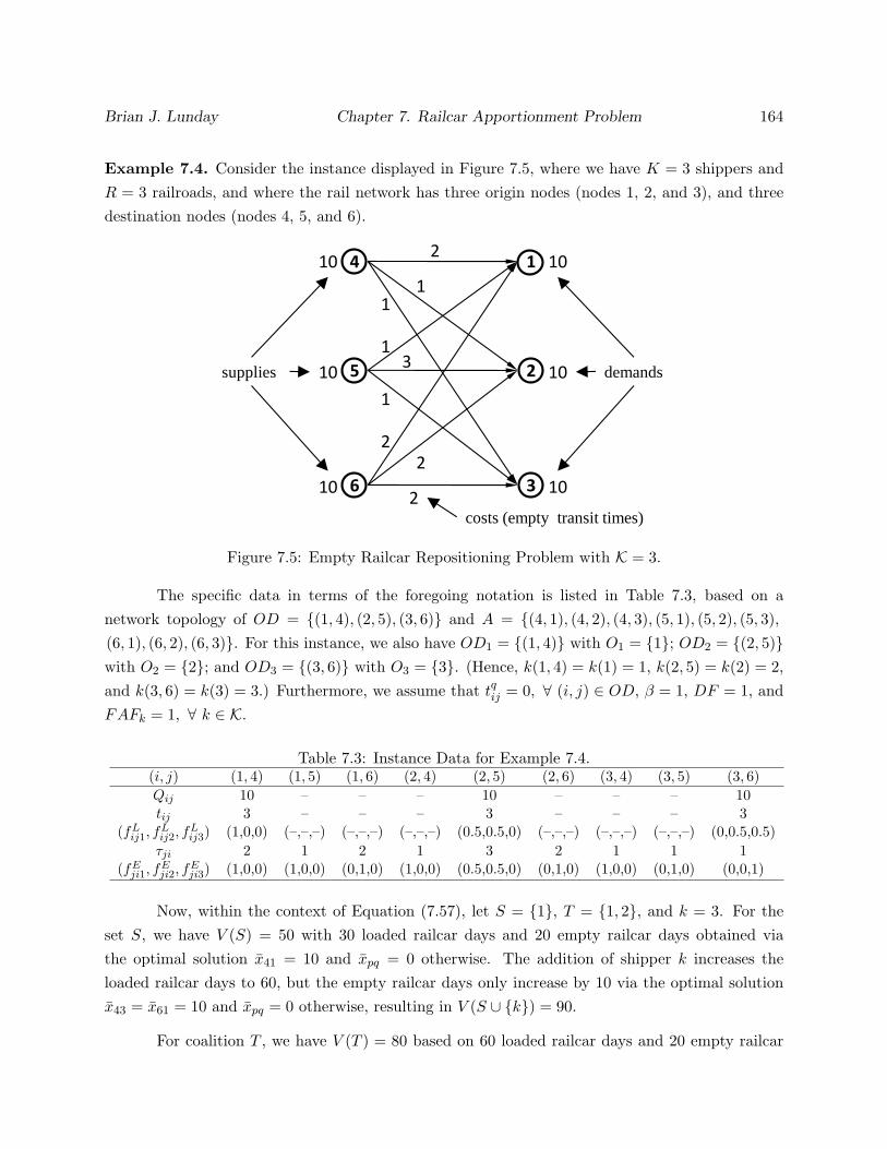
Brian J. Lunday Chapter 7. Railcar Apportionment Problem 164
Example 7.4. Consider the instance displayed in Figure 7.5, where we have K = 3 shippers andR = 3 railroads, and where the rail network has three origin nodes (nodes 1, 2, and 3), and threedestination nodes (nodes 4, 5, and 6).
4
5
1 10
2 10
10
10 demands
6 3 1010
2
3
1
2
2
2
1
1
1
supplies
costs (empty transit times)
Figure 7.5: Empty Railcar Repositioning Problem with K = 3.
The specific data in terms of the foregoing notation is listed in Table 7.3, based on anetwork topology of OD = (1, 4), (2, 5), (3, 6) and A = (4, 1), (4, 2), (4, 3), (5, 1), (5, 2), (5, 3),(6, 1), (6, 2), (6, 3). For this instance, we also have OD1 = (1, 4) with O1 = 1; OD2 = (2, 5)with O2 = 2; and OD3 = (3, 6) with O3 = 3. (Hence, k(1, 4) = k(1) = 1, k(2, 5) = k(2) = 2,and k(3, 6) = k(3) = 3.) Furthermore, we assume that tqij = 0, ∀ (i, j) ∈ OD, β = 1, DF = 1, andFAFk = 1, ∀ k ∈ K.
Table 7.3: Instance Data for Example 7.4.(i, j) (1, 4) (1, 5) (1, 6) (2, 4) (2, 5) (2, 6) (3, 4) (3, 5) (3, 6)Qij 10 – – – 10 – – – 10tij 3 – – – 3 – – – 3
(fLij1, f
Lij2, f
Lij3) (1,0,0) (–,–,–) (–,–,–) (–,–,–) (0.5,0.5,0) (–,–,–) (–,–,–) (–,–,–) (0,0.5,0.5)
τji 2 1 2 1 3 2 1 1 1(fE
ji1, fEji2, f
Eji3) (1,0,0) (1,0,0) (0,1,0) (1,0,0) (0.5,0.5,0) (0,1,0) (1,0,0) (0,1,0) (0,0,1)
Now, within the context of Equation (7.57), let S = 1, T = 1, 2, and k = 3. For theset S, we have V (S) = 50 with 30 loaded railcar days and 20 empty railcar days obtained viathe optimal solution x41 = 10 and xpq = 0 otherwise. The addition of shipper k increases theloaded railcar days to 60, but the empty railcar days only increase by 10 via the optimal solutionx43 = x61 = 10 and xpq = 0 otherwise, resulting in V (S ∪ k) = 90.
For coalition T , we have V (T ) = 80 based on 60 loaded railcar days and 20 empty railcar
Brian J. Lunday Chapter 7. Railcar Apportionment Problem 165
days obtained via the optimal solution x42 = x51 = 10 and xpq = 0 otherwise, whereas V (T ∪k) =130 with 90 loaded railcar days and 40 empty railcar days, resulting via the optimal solutionx42 = x51 = x63 = 10 and xpq = 0 otherwise. Therefore, this instance manifests
V (S ∪ k)− V (S) = 40 < 50 = V (T ∪ k)− V (T ),
and so (7.57) is violated, and the characteristic function defined by (7.56) is not submodular.
Remark 7.2. Because V (·) defined by (7.56) is not submodular, convexity is not assured, andit is possible that the Shapely-valued shipper allocations lie outside the core, or that the coremay even be empty, resulting in an unstable grand coalition K. However, in practice, the grandcoalition is contractually enforced, and so we retain the Shapley-valued shipper allocations amongour alternative schemes considered for comparative testing in Section 7.6.
Based on (7.56), we may restate (7.54) equivalently as:
φ(3)k (V ) =
∑S⊆KS⊇k
(|S| − 1)!(K − |S|)!K!
(FSS − FSS\k
), ∀ k ∈ K. (7.58)
Within our context, Equation (7.58) represents the expected allocation of empty railcars attributedto shipper k due to its presence in the overall pooling agreement. Accordingly, we propose thefollowing shipper allocation rule (SA4), with FSSA4(k), for k ∈ K, denoting the allocation of fleetFS to shipper k:
FSSA4(k) ≡ φ(3)k (V ). (7.59)
Note that, given (7.59) and (7.55), we have∑k∈K
FSSA4(k) = FS, (7.60)
as required.
As an illustration, consider the application of SA4 to the instance presented in Example7.4. Table 7.4 lists, for all S ⊆ K, the optimal fleet sizes (and unique solutions thereof) used tocompute the Shapley values for shippers k ∈ K.

Brian J. Lunday Chapter 7. Railcar Apportionment Problem 166
Table 7.4: Optimal Fleet Sizes for S ⊆ K.S FSS Non-zero xpq-values∅ 0 ∅1 50 x41 = 102 60 x52 = 103 50 x63 = 101,2 80 x42 = x51 = 101,3 90 x43 = x61 = 102,3 90 x53 = x62 = 101,2,3 130 x42 = x51 = x63 = 10
We may now apply Equations (7.59) and (7.58) directly to determine the shipper allocationsas follows:
FSSA4(1) =(1/3)(FS1 − FS∅) + (1/6)(FS1,2 − FS2)+
+ (1/6)(FS1,3 − FS3) + (1/3)(FS1,2,3 − FS2,3)
=(50/3) + (20/6) + (40/6) + (40/3) = 40,
FSSA4(2) =(1/3)(FS2 − FS∅) + (1/6)(FS1,2 − FS1)+
+ (1/6)(FS2,3 − FS3) + (1/3)(FS1,2,3 − FS1,3)
=(60/3) + (30/6) + (40/6) + (40/3) = 45,
FSSA4(3) =(1/3)(FS3 − FS∅) + (1/6)(FS1,3 − FS1)+
+ (1/6)(FS2,3 − FS2) + (1/3)(FS1,2,3 − FS1,2)
=(50/3) + (40/6) + (30/6) + (50/3) = 45,
which contrasts from the shipper allocations of FSPAS(1) = FSPAS(2) = 40 and FSPAS(3) = 50obtained by applying the current industry practice to the same instance.
A notable disadvantage to SA4 is computational complexity. It requires 2K − 1 fleet-sizing computations for a consortium of K shippers. Given K = 9 shipers, this involves thesolution of 29 − 1 = 511 transportation problems (of varying sizes). However, the Shapley-valueallocation technique has a respectable basis in game theory, and could be utilized variously bydefining characteristic functions that measure the coalition value based on travel time, total time,railcar mileage, shipping costs, or a weighted combination of any of these metrics.

Brian J. Lunday Chapter 7. Railcar Apportionment Problem 167
7.5 Alternative Approaches for Carrier Allocations
In this section, we first demonstrate the equivalence of the current industry practice for carrierallocations to a game-theoretic Shapley-value based approach, and next propose an alternativetechnique based on considering total capital plus operating costs, as opposed to just capital costs,when determining proportionality factors for conducting railcar allocations. We denote FSRAδ
r
to be the allocation of railcars under railroad allocation scheme δ (i.e., under RAδ) to railroad r,for all δ = 1, 2, r ∈ R, where for δ = 1, we have FSRA1
r ≡ FSPASr , ∀ r ∈ R.
7.5.1 Loaded Railcar-days of Business
As discussed in Section 7.2.2 under the existing scheme PAS, the current industry standard allocatesrailcars to railroads by apportioning each shipper’s assigned railcars in proportion to the loadedrailcar-days of business conducted with each railroad. More specifically, Equation (7.13) allocatesshipper k’s allotment of empty railcars FSPAS(k) to each carrier, where the total allocation toeach carrier is then determined by summing the corresponding allocations over all shippers as inEquation (7.14). Naturally, the same allocation process described by Equations (7.13) and (7.14)can be utilized to assign railcars to railroads based on any of the foregoing shipper allocationmechanisms, SAα, α = 1, 2, 3, 4. We denote such a carrier allocation scheme as RA1 for notationaldistinction from the shipper allocation method PAS, while noting that FSRA1
r ≡ FSPASr , ∀ r ∈ R.
It is insightful to note that the allocation scheme RA1 is in fact a game-theoretic approachbased on Shapely value allocations. To see this, consider any shipper k ∈ K, and examine thefollowing process to allocate the shipper’s assigned railcars FS(k) (as determined by FSPAS(k) orFSSAα
k , α = 1, 2, 3, 4) to the set of carriers r ∈ R. Define a characteristic function on the powerset T ⊆ R as given by:
V k (T ) =∑r∈T
Lrk, ∀ T ⊆ R, (7.61)
where Lrk is defined by Equation (7.11). Thus, we have
V k (R) =∑r∈R
Lrk =∑∑
(i,j)∈ODk
Qijtij , (7.62)
which represents the total loaded railcar-days associated with shipper k, as in (7.12). The corre-sponding Shapley value allocation factor is given by
φkr (V
k) =∑
T⊆RT⊇r
(|T | − 1)!(R− |T |)!R!
[V k (T )− V k (T\r)
], ∀ r ∈ R, (7.63)
Brian J. Lunday Chapter 7. Railcar Apportionment Problem 168
which represents the expected contribution to railcar-days of shipment by carrier r in support ofshipper k, considered with equal probability with respect to each of the possible coalition formationsamong the carriers. Accordingly, noting (7.62), (7.63), and that
∑r∈R
φkr (V
k) = V k(R), the Shapley
value allocation concept would prescribe shipper k’s assigned railcars to carrier r in proportion toφk
r (Vk) as follows:
FS′rk = FS(k)
φkr (V
k)∑ρ∈R
Lρk
, ∀ r ∈ R. (7.64)
Proposition 7.4. Given any set of shipper allocations FS(k), ∀ k ∈ K, the game-theoretic shipper-to-carrier allocations FS′rk computed via (7.64) precisely match the allocations FSrk, ∀ r ∈ R, ascorrespondingly prescribed by (7.13) using the current industry practice.
Proof. For any k ∈ K, considering V k(T ) as defined in (7.61), we have that[V k (T )− V k (T\r)
]≡
Lrk, ∀ r ⊆ T ⊆ R. Using this identity in (7.63), we obtain φkr (V
k) = Lrk, ∀ r ∈ R, k ∈ K, which,when substituted into (7.64), yields FS′rk = FSrk by Equation (7.13), for all r ∈ R, k ∈ K.
Moreover, due to the equivalence of RA1 to the game-theoretic Shapley-value allocationscheme based on the characteristic function (7.61), Proposition 7.5 below demonstrates the stabilityof the coalition of carriers under RA1.
Proposition 7.5. The game defined by the characteristic function V k(·) of Equation (7.61) isconvex, and hence its core C ′(V k) is nonempty and the Shapley value allocation factor (7.63)belongs to the core.
Proof. To show that the game defined by V k(·) is convex, it is sufficient to establish the submod-ularity of V k(·), which may be identified by the condition (Dresden, 1988):
V k(S ∪ r)− V k(S) ≥ V k(T ∪ r)− V (T ), ∀ S ⊆ T ⊆ R\r, ∀ r ∈ R. (7.65)
Utilizing (7.61) and (7.11), the components of (7.65) are given by
V k(S ∪ r)− V k(S) =∑
ρ∈S∪r
Lρk −∑ρ∈S
Lρk =∑∑
(i,j)∈ODk
fLijrQijtij , (7.66)
and likewise,
V k(T ∪ r)− V (T ) =∑
ρ∈T∪r
Lρk −∑ρ∈T
Lρk =∑∑
(i,j)∈ODk
fLijrQijtij . (7.67)
Brian J. Lunday Chapter 7. Railcar Apportionment Problem 169
Hence, equality holds in (7.65) and therefore the game is convex. Consequently, as per Shapley(1971), the core C ′(V k) is nonempty, and the Shapley value allocation factor (7.63) belongs to thecore.
7.5.2 Total Capital Plus Operating Costs
In this section, we propose an alternative scheme RA2 in which we determine fleet allocationsfor each railroad (denoted FSRA2
r , ∀ r ∈ R) based on an equitable distribution of total capitalplus operating costs, while examining the entire pool of railcars as a whole, as opposed to firstdetermining shipper allocations and then apportioning these to railroads via (7.13) and (7.14).
Accordingly, consider the following notation:
• c: annualized capital cost of each railcar.
• cEpqr: annual cost associated with the corresponding empty railcar-days fEpqrτpqxpq (per day,
on average) spent by railroad r on route (p, q), ∀ r ∈ R, (p, q) ∈ A. We further assume cEpqr
to be linearly proportional to fEpqrτpqxpq at a marginal rate of cEM
pqr dollars per year per emptyrailcar-days, for all (p, q) ∈ A, r ∈ R, i.e., cEpqr ≡ cEM
pqr fEpqrτpqxpq, ∀ (p, q) ∈ A, r ∈ R.
• ξr ≡∑∑(p,q)∈A
cEpqr: annual total empty railcar movement cost incurred by railroad r on the
network, ∀ r ∈ R.
• FSRA2r : fleet size allocated to railroad r under scheme RA2, ∀ r ∈ R.
Then, defining Lrk as in Equation (7.11) to represent the total loaded railcar-days of businessthat railroad r conducts with shipper k, suppose that we compute values fr such that∑
r∈Rfr = FS, (7.68)
and such that, measured per annum, the total capital plus operating costs for the railroads r ∈ R,are directly proportional to their respective total loaded railcar-days of business, that is,
ξr + cfr = σ∑k∈K
Lrk, ∀ r ∈ R, (7.69)
Brian J. Lunday Chapter 7. Railcar Apportionment Problem 170
where σ is some proportionality constant. From (7.68) and (7.69), we obtain
fr =
σ∑k∈K
Lrk − ξr
c
, ∀ r ∈ R, where, σ =
c(FS) +
∑r∈R
ξr∑r∈R
∑k∈K
Lrk
. (7.70)
Note that since fr could be negative in (7.70) for railroads that perform a disproportionate amountof empty railcar movements as compared with the loaded business they conduct, the final allocationsare prescribed according to a feasible least squares deviation from the fr-values as determined bythe following problem:
Minimize
∑r∈R
(fr − fr)2 :∑r∈R
fr = FS; fr ≥ 0, ∀ r ∈ R
. (7.71)
Problem (7.71) can be solved efficiently using the variable dimension method described in Bitranand Hax (1976) and Sherali and Shetty (1980). Letting f∗r , r ∈ R, denote the optimal solutionobtained for Problem (7.71), we let FSRA2
r ≡ f∗r , r ∈ R.
Remark 7.3. The above scheme is independent of the shipper allocations (determined via anymechanism such as PAS or SAα, α = 1, 2, 3, 4), and assumes the authority of a central organization,e.g., the TTX Reload Group, to perform the railroad allocations. At present such an authoritydoes not exist, and each shipper k must individually assign its allocated fleet FS(k) among therailroads with which it conducts business.
We demonstrate the application of RA1 to the instance depicted in Example 7.1, with thefollowing additional assumptions:
• The marginal costs are uniform at cEMpqr ≡ $3650, ∀ (p, q) ∈ A, r ∈ R, based on $10 per
empty railcar-day and a planning factor of 365 shipping days per year.
• The net present cost of a railcar is P =$100,000, which incorporates annual operations andmaintenance costs.
• The expected life of a railcar is N = 20 years.
• The effective annual discount rate on the value of the railcar is ieff = 10%.
First, we compute the annualized capital cost of each railcar to be
c = Pieff (1 + ieff )N
(1 + ieff )N − 1= $11745.96. (7.72)

Brian J. Lunday Chapter 7. Railcar Apportionment Problem 171
Applying the assumed linear proportionality factors, we determine ξr, ∀ r = 1, 2, as
ξ1 =∑∑(p,q)∈A
cEMpq1 f
Epq1τpqxpq = 3650 [1(1)15 + 1(1)0 + 0(2)10 + 0.5(2)12] = 98550, (7.73)
ξ2 =∑∑(p,q)∈A
cEMpq2 f
Epq2τpqxpq = 3650 [0(1)15 + 0(1)0 + 1(2)10 + 0.5(2)12] = 116800. (7.74)
Next, we utilize Equations (7.70) and (7.72)–(7.74), as well as the previously determined fleet sizeFS = 106 and loaded railcar-days Lrk, ∀ r = 1, 2, k = 1, 2, to calculate a σ-value of
σ =[11745.96(106) + (98550 + 116800)
(15 + 6 + 20 + 6)
]= 31072.81,
thus yielding
f1 =31072.81(15 + 6)− 98550
11745.96= 47.16, (7.75)
f2 =31072.81(20 + 6)− 116800
11745.96= 58.84. (7.76)
Since, fr ≥ 0, ∀ r = 1, 2, we can conclude by inspection of (7.71) that FSRA21 = 47.16 and
FSRA22 = 58.84, differing from the respective allocations of 48 and 58 railcars via the current
industry standard demonstrated in Example 7.1. (Note that if we further restricted fr, ∀ r ∈ R,to integer-values within (7.71), we would attain FSRA2
1 = 47 and FSRA21 = 59 instead.)
7.6 Computations and Comparisons
In this section, we apply each of the 10 combinations of five shipper and two carrier allocationtechniques to instances that are representative of the TTX Reload Group problem. Using thecurrent industry practice as a benchmark, we compare and analyze the results in order to provideinsights into selecting an appropriate combination of allocation techniques for implementation bythe TTX Reload Group.
The test-bed of problem instances were generated as follows to simulate realistic scenariosaccording to guidelines provided by TTX. First, we determined integer-valued numbers of shippersK ∈ U [14, 20], carriers R ∈ U [6, 12], origin nodes m ∈ U [40, 80], and destination nodes n ∈U [60, 120], where U [·, ·] denotes an integer-valued uniform distribution on [·, ·]. To provide variabilityamong shippers, we assumed that the top, middle, and bottom tiers of shippers, each consisting ofapproximately one third of the pool, ship loaded railcars from 50%, 30%, and 20% of all origins,with the origins assigned to shippers within each tier with equal probabilities, while ensuring that
Brian J. Lunday Chapter 7. Railcar Apportionment Problem 172
each shipper is associated with at least one origin node. We next generated arcs for loaded flowsbased on the assumption that each origin ships to between 5% and 85% of the destinations, as perSherali and Tuncbilek (1997). Upon generating an integer-valued demand on U [20, 40] for loadedrailcars at each destination j ∈ J , we determined the loaded flows Qij via a uniform distributionamong the possible origin nodes, such that
∑i∈I
Qij is equal to the demand for loaded railcars at node
j, for all j ∈ J , and with the additional provision that maxi:(i,j)∈OD
Qij ≤ 4 mini:(i,j)∈OD
Qij , ∀ j ∈ J ,
in order to prevent disproportionate non-zero loaded flows into a destination from any origin node(Sherali and Tuncbilek, 1997). As per Sherali and Tuncbilek (1997), we generated integral tij-values for all (i, j) ∈ OD on the interval [1, 6]. The normal practice in the industry seeks to limitempty railcar traffic to a set of prescribed routes, opening new routes as necessary to accommodateflow. We modeled this by assuming a complete bipartite graph for the return flow arcs (p, q) ∈ A,with τpq = τF
qptqp for (q, p) ∈ OD, where τFqp ∈ U [1.5, 2.0] is a multiplicative factor, and with
τpq ∈ U [2.0, 12.0] for (q, p) /∈ OD, combined with the imposition of flow capacities(
3 max(i,j)∈OD
Qij
)on all the empty railcar routes (j, i) ∈ A. Furthermore, we determined tqij ∈ U [1.5, 2.5], ∀ (i, j) ∈OD, using the nearest-tenth value. In order to determine fL
ijr, ∀ (i, j) ∈ OD, r ∈ R, and affectheterogeneity in the carrier fleet, we assumed that the top, middle, and bottom tiers of carriers,each consisting of approximately one-third of the pool, conduct 50%, 30%, and 20% of all loadedrailcar flow business, and we further distributed these aggregated proportions uniformly amongOD paris to compute the fL
ijr-values within each tier, at a resolution granularity of 0.1%. Wedetermined fE
pqr, ∀ (p, q) ∈ A, r ∈ R, in the same manner, obviating the possiblity of a carrierconducting business only for transporting empty railcars, as the majority of such short-haul carriersare involved only as separate subcontractors to carriers in the pooling agreement. All instancesincorporated a bad-order factor of β = 1.03, and a dynamic factor DF ∈ U [1.10, 1.30], as supportedby historical data provided by the TTX Reload Group. We generated forecast accuracy factorsFAFk ∈ U [0.95, 1.05], ∀ k ∈ K. For the implementation of carrier allocation method RA2, weassumed a railcar net present cost of P =100,000 dollars, with a life of N = 20 years and an effectiveannual interest rate of ieff = 10%. We generated the cEM
pqr -values on U [3400, 3800], ∀ (p, q) ∈ A, forcarriers belonging to the first tier that transport 50% of the loaded railcars to allow for variabilitydue to wear-and-tear on routes. Assuming that a greater volume of business reduces marginaloperating costs, we accordingly generated the cEM
pqr -values for carriers in the 30% and 20% tiers ofloaded railcar business to be 10% and 25% greater, respectively, than the marginal costs for the tierconducting 50% of the loaded movements. Finally, based on current practice, we utilized Equation(7.7) instead of (7.8) to size the railcar fleet while accounting for dynamic fluctuations and forecastaccuracies, pending a revised adoption by the industry. We coded all allocation methods in C++,invoking CPLEX 11.1 via Concert Technology to solve the different optimization subproblems. Allruns were executed on a computer with an Intel 2.33 GHz Xeon Processor and 3.25 GB of RAM.
Brian J. Lunday Chapter 7. Railcar Apportionment Problem 173
Tables 7.5 and 7.6 report the prescribed railcar allocations FS(k) for shippers, ∀ k ∈ K,and the allocations FSr for carriers, ∀ r ∈ R, respectively, for each of the 10 methodologicalcombinations, along with the required computational effort (measured in CPU seconds), as appliedto a sample instance generated via C++ (for seed #1, which induces m = 60 and n = 86). Inthe rightmost columns of Tables 7.5 and 7.6, we present the mean and standard deviation for eachshipper and carrier allocation, respectively, in order to illustrate the variability of allocations acrossmethodologies for a given coalition participant. Compared to the shipper allocations prescribed byPAS, allocation methods SA1, SA2, and SA3 acted in a similar manner for each shipper, k ∈ K, withregard to either increasing or decreasing the respective railcar allocation, with the exception of oneshipper (k = 12), for which SA2 decreased the railcar allocation by 0.0066%, while SA1 and SA3increased it by 0.20% and 0.046%, respectively. In contrast, SA4 adjusted shipper allocations fromthe PAS prescriptions in the opposite manner from SA1, SA2, and SA3 for 13 of the 20 shippers.Unlike the shipper allocations, the carrier allocations exhibited relatively lesser variance overallamong the 10 combinations. While SA1, SA2, and SA3 required increasingly more computationaleffort compared to PAS, the net increase in effort in combination with either carrier allocationmethod RA1 or RA2 was no more than 2 CPU seconds. In contrast, the implementation of SA4 incombination with either RA1 or RA2 required a significant increase in computational effort fromthe current practice that utilizes PAS and RA1, although the effort of just under 5.5 CPU hoursis not necessarily prohibitive for implementation. In general, we note that the railcar allocationsfor this instance exhibit more variability for shippers among the five shipper allocation schemes, asreported in Table 7.5, than for carriers among the six distinct shipper and carrier allocation methodcombinations (with RA2 allocations being independent of any given shipper allocation method), asreported in Table 7.6.
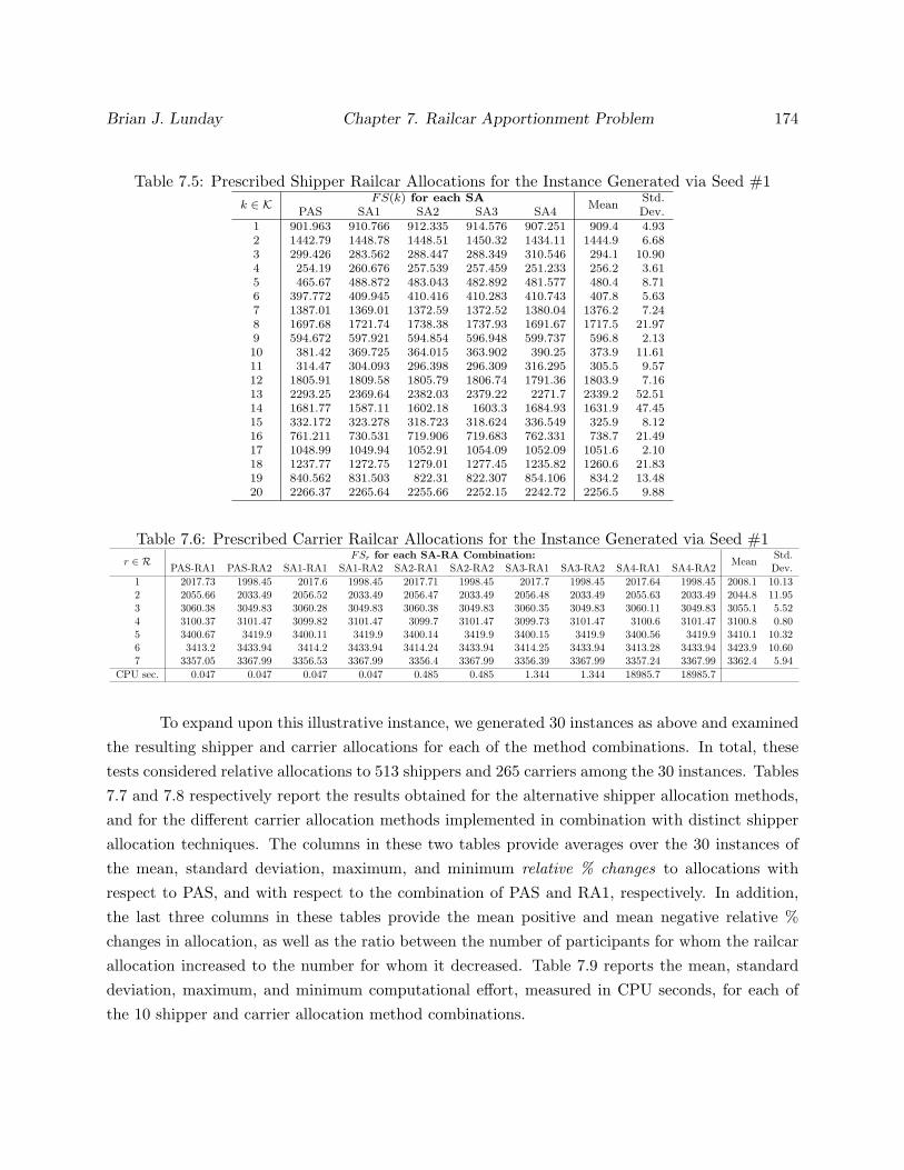
Brian J. Lunday Chapter 7. Railcar Apportionment Problem 174
Table 7.5: Prescribed Shipper Railcar Allocations for the Instance Generated via Seed #1k ∈ K FS(k) for each SA
MeanStd.
PAS SA1 SA2 SA3 SA4 Dev.1 901.963 910.766 912.335 914.576 907.251 909.4 4.932 1442.79 1448.78 1448.51 1450.32 1434.11 1444.9 6.683 299.426 283.562 288.447 288.349 310.546 294.1 10.904 254.19 260.676 257.539 257.459 251.233 256.2 3.615 465.67 488.872 483.043 482.892 481.577 480.4 8.716 397.772 409.945 410.416 410.283 410.743 407.8 5.637 1387.01 1369.01 1372.59 1372.52 1380.04 1376.2 7.248 1697.68 1721.74 1738.38 1737.93 1691.67 1717.5 21.979 594.672 597.921 594.854 596.948 599.737 596.8 2.1310 381.42 369.725 364.015 363.902 390.25 373.9 11.6111 314.47 304.093 296.398 296.309 316.295 305.5 9.5712 1805.91 1809.58 1805.79 1806.74 1791.36 1803.9 7.1613 2293.25 2369.64 2382.03 2379.22 2271.7 2339.2 52.5114 1681.77 1587.11 1602.18 1603.3 1684.93 1631.9 47.4515 332.172 323.278 318.723 318.624 336.549 325.9 8.1216 761.211 730.531 719.906 719.683 762.331 738.7 21.4917 1048.99 1049.94 1052.91 1054.09 1052.09 1051.6 2.1018 1237.77 1272.75 1279.01 1277.45 1235.82 1260.6 21.8319 840.562 831.503 822.31 822.307 854.106 834.2 13.4820 2266.37 2265.64 2255.66 2252.15 2242.72 2256.5 9.88
Table 7.6: Prescribed Carrier Railcar Allocations for the Instance Generated via Seed #1r ∈ R FSr for each SA-RA Combination:
MeanStd.
PAS-RA1 PAS-RA2 SA1-RA1 SA1-RA2 SA2-RA1 SA2-RA2 SA3-RA1 SA3-RA2 SA4-RA1 SA4-RA2 Dev.1 2017.73 1998.45 2017.6 1998.45 2017.71 1998.45 2017.7 1998.45 2017.64 1998.45 2008.1 10.132 2055.66 2033.49 2056.52 2033.49 2056.47 2033.49 2056.48 2033.49 2055.63 2033.49 2044.8 11.953 3060.38 3049.83 3060.28 3049.83 3060.38 3049.83 3060.35 3049.83 3060.11 3049.83 3055.1 5.524 3100.37 3101.47 3099.82 3101.47 3099.7 3101.47 3099.73 3101.47 3100.6 3101.47 3100.8 0.805 3400.67 3419.9 3400.11 3419.9 3400.14 3419.9 3400.15 3419.9 3400.56 3419.9 3410.1 10.326 3413.2 3433.94 3414.2 3433.94 3414.24 3433.94 3414.25 3433.94 3413.28 3433.94 3423.9 10.607 3357.05 3367.99 3356.53 3367.99 3356.4 3367.99 3356.39 3367.99 3357.24 3367.99 3362.4 5.94
CPU sec. 0.047 0.047 0.047 0.047 0.485 0.485 1.344 1.344 18985.7 18985.7
To expand upon this illustrative instance, we generated 30 instances as above and examinedthe resulting shipper and carrier allocations for each of the method combinations. In total, thesetests considered relative allocations to 513 shippers and 265 carriers among the 30 instances. Tables7.7 and 7.8 respectively report the results obtained for the alternative shipper allocation methods,and for the different carrier allocation methods implemented in combination with distinct shipperallocation techniques. The columns in these two tables provide averages over the 30 instances ofthe mean, standard deviation, maximum, and minimum relative % changes to allocations withrespect to PAS, and with respect to the combination of PAS and RA1, respectively. In addition,the last three columns in these tables provide the mean positive and mean negative relative %changes in allocation, as well as the ratio between the number of participants for whom the railcarallocation increased to the number for whom it decreased. Table 7.9 reports the mean, standarddeviation, maximum, and minimum computational effort, measured in CPU seconds, for each ofthe 10 shipper and carrier allocation method combinations.

Brian J. Lunday Chapter 7. Railcar Apportionment Problem 175
Table 7.7: Relative Changes (%) to Shipper Allocations for Alternative Methods.
MeanStd.
Max. Min.Mean Mean Inc:Dec
Dev. Pos. Neg. RatioSA1 0.095 2.997 5.209 -4.805 2.519 -2.444 1.119SA2 0.096 2.880 4.904 -4.737 2.424 -2.362 1.142SA3 0.092 2.884 4.917 -4.763 2.399 -2.392 1.164SA4 0.518 1.891 4.564 -2.378 1.754 -1.095 1.389
Table 7.8: Relative Changes (%) to Carrier Allocations for Alternative Shipper and Carrier Allo-cation Method Combinations.
MeanStd.
Max. Min.Mean Mean Inc:Dec
Dev. Pos. Neg. RatioSA1-RA1 -0.0003 0.024 0.035 -0.036 0.019 -0.019 1.074SA2-RA1 -0.0003 0.023 0.033 -0.036 0.019 -0.018 1.011SA3-RA1 -0.0003 0.023 0.033 -0.036 0.018 -0.018 1.016SA4-RA1 0.0001 0.015 0.023 -0.023 0.012 -0.013 1.225PAS-RA2,SAα-RA2, -0.1536 0.703 0.625 -1.206 0.471 -0.655 0.859α = 1, ..., 4
Table 7.9: Computational Effort (CPU Seconds) for Shipper and Carrier Allocation Method Com-binations.
MeanStd.
Max. Min.Dev.
PAS-RA1 0.0616 0.0460 0.2820 0.0310PAS-RA2 0.0620 0.0462 0.2820 0.0310SA1-RA1 0.0633 0.0496 0.2980 0.0310SA1-RA2 0.0644 0.0494 0.2980 0.0160SA2-RA1 0.4373 0.1071 0.7340 0.2190SA2-RA2 0.4362 0.1086 0.7340 0.2030SA3-RA1 1.405 0.5366 2.750 0.6410SA3-RA2 1.404 0.5376 2.750 0.6410SA4-RA1 5484 6265 20322 198.9SA4-RA2 5484 6265 20322 198.9
From Tables 7.7 and 7.8, we note the greater variability among relative % changes forshipper allocations than for carrier allocations under alternative methods, on average, as well asfor the minimum and maximum relative % changes to allocations. The positive or negative relative% changes in allocations for shippers averages between 1.09% and 2.52%, compared to less than0.66% for carriers. Therefore, we focus our discussion below on the consideration of alternativeshipper allocation methods, noting that the potential effect on coalition members is greater in thiscase.

Brian J. Lunday Chapter 7. Railcar Apportionment Problem 176
As reported in Table 7.7, observe that under each alternative shipper allocation method,more automobile shippers encountered an increase in their railcar allocations, compared to thosewhose allocations decreased. This ratio is notably larger under method SA4, compared to methodsSA1–SA3, occurring at a ratio that approaches 14 increases for every 10 decreases. Ultimately, it isthe philosophy of shipper allocation methods SA1–SA4 that needs to be embraced, as any of themaffect an equitable allocation, albeit via different conceptual measures. Within this context, theempirically higher average ratios for shippers in Table 7.7 under allocation method SA4, given itsrelatively more elaborate consideration of shipper contributions, suggests that several participantsshould support a greater capital allocation burden than currently effected under PAS allocations.
From Table 7.8, there exists a much smaller variability in carrier allocations for methodRA1, when applied with any of the shipper allocation methods, than for method RA2. Consideringthe alternative shipper allocation methods in combination with carrier allocation method RA1,the ratio of increases to decreases in allocations, compared to the current industry technique,is again larger for SA4 than for SA1–SA3. In contrast, carrier allocation method RA2 affects,on average, a greater number of carriers that encounter decreases in allocations than those whoencounter increases. In combination with the more elaborate consideration of shipper contributionsvia SA4, the carrier allocation techniques RA1 and RA2 respectively yield the maximum andminimum increase-decrease ratios of 1.225 and 0.859 in Table 7.8, suggesting empirical evidencethat a redistribution of the capital allocation burden is also in order for carriers.
Considering the computational effort for the shipper and carrier allocation method com-binations as presented in Table 7.9, although the techniques involving SA4 are relatively morecomputationally intensive, the run-times are yet quite reasonable from the viewpoint of strategicplanning. Also, note that the average computational effort for the method combination SA4-RA1was 1.52 CPU hours over the 30 instances, but only 41.0 CPU minutes when restricted to the fourinstances involving 17 shippers, a problem size that is consistent with the current set of shippersin the coalition managed by the TTX Reload Group.
7.7 Conclusions and Recommendations
In this chapter, we have demonstrated potential inequities in the current railcar allocation practices,and have proposed four alternative shipper allocation methods and one alternative carrier allocationtechnique, and conducted extensive computational tests that demonstrate the variations in suchallocation mechanisms. Based on our analysis, we propose two mandates for change to the currentindustry practice. First, as discussed in Section 7.3, the fleet sizing problem, and subsequentrailcar allocation problems, should be disaggregated into disjoint subproblems based on each of the

Brian J. Lunday Chapter 7. Railcar Apportionment Problem 177
separable components in the railcar transportation network. Second, the currently implementedshipper allocation technique, which is based on associated O-D pair allocations that accrue from anestimate of a weighted average empty return time to the corresponding origin, should be abandoneddue to the potential inequities of the type demonstrated in Section 7.4.1, arising from possiblealternative optimal return flow solutions.
Given the need for a change in current shipper allocation practices, we have proposed eightalternative shipper-and-carrier allocation method combinations. Although the different conceptualparadigms can produce different railcar allocations, it is the philosophy of each allocation schemethat needs to be embraced by the coalition participants, in that any of these proposed alternativeseliminates potential for inequities inherent in the current industry practice. Shipper allocationmethod SA1 directly addresses the inequity demonstrated in Section 7.4.1 by considering allocationsproportional to loaded transit plus queuing times. Methods SA2 and SA3 allocate railcars toshippers based on their marginal value to the coalition, computed shipper-wise or with respect toeach origin node of a shipper, respectively. In comparison, method SA4 more elaborately considersthe contributions of each shipper to the coalition in a game-theoretic context via a Shapley valuethat computes an expected contribution based on all possible permutations of coalition formation,given the existence of a grand coalition. For carrier allocations, our proposed method RA2 has meritin its consideration of capital plus operating costs. While any of these alternative combinations ofshipper and carrier allocation methods is philosophically preferable to the current practice, we donote that the allocation method combination of SA4-RA1 has appeal in uniformity in approach, inthat, by Proposition 7.4, RA1 is also based on Shapley values. Moreover, the increase-to-decreaseratios indicate that, for both shippers and carriers alike, a redistribution of the capital allocationburden from current levels might be appropriate.
However, because the determination of railcar allocations by the TTX Reload Group isonly a precursor to a negotiated settlement, we recognize that the recommendation of an alterna-tive allocation method is not a prescription, per se. Nevertheless, any of the proposed allocationmechanisms affords a more philosophically equitable approach, from which coalition members maybargain. Indeed, the alternative methods could be used to determine a range of equitable alloca-tions, which could then serve as the basis for negotiation within the pooling agreement.
For future research, alternative methods could be considered that are more directly cost-based in nature. In a capitalist economy, equity among coalition participants should generally bemeasured in monetary terms. Although the current and proposed measures are both cost related,a direct conversion may provide additional resolution, because any single loaded railcar-day maynot be of equal monetary value among shippers, given the relative values of the automobiles beingtransported. When such direct monetary measures cannot be determined, an equivalent metricbased on time or physical capital might serve as a suitable substitute, depending on the collective

Brian J. Lunday Chapter 7. Railcar Apportionment Problem 178
consent of the coalition participants.

Chapter 8
Conclusions and Directions for Future
Research
In this dissertation we have examined several resource allocation problems on networks pertainingto combating terrorism, which deal with interdicting either the net flow or a single unit of flowattempting to traverse a network, as well as pertaining to the allocation of a pooled railcar fleetamong participants in an automobile shipping consortium, and have developed effective models andsolution procedures for these problems.
As part of an effort to consider a broader scope of resource coordination, we examined inChapter 3 the Nested Event Tree Optimization problem, wherein we seek to combat terrorism viathe coordinated allocation of countermeasure and consequence management resources in order tominimize the expected risk of a terrorist organization and its development of capabilities, in con-junction with the subsequent use of such capabilities to attack targets and affect specific outcomes.We modeled this problem as a nonconvex factorable program, and we developed and applied threeconceptual approaches, with two variants each, for designing customized algorithms. Our firsttwo solution techniques respectively construct convex and linear relaxations to the original prob-lem, each of which is embedded within a branch-and-bound framework that we prove attains anε-optimal solution with finite computational effort. We further enhanced these branch-and-boundsolution methods by incorporating suitable branching and partitioning strategies, while invokingrange reduction techniques. Our third approach constructs MIP approximations to represent thenonlinearities inherent within the model formulation, and we demonstrated its ability to boundthe maximum error of the resulting solution from the global optimum based on the granularityof the approximation. For each of these three methodologies, we constructed the relaxations andthe proposed MIP approximation in an alternative parameter space, where the latter was fur-
179
Brian J. Lunday Chapter 8. Conclusions and Directions for Future Research 180
ther demonstrated to yield a valid lower bound on the original formulation, which facilitates thecomputations of an optimality gap. Over a test bed of problem instances, we demonstrated thatall proposed techniques significantly improve upon the performance of the commercial softwareBARON, with the MIP approximation approach providing superlative results, yielding an averageoptimality gap of 0.35% (compared to 4.29% for BARON) with a corresponding speed-up factor ofabout 33. The import of our model and accompanying solution procedures lie in their suitabilityfor higher level strategic planning for resource deployment and, in addition to optimally allocatingexisting resources within budgetary constraints, have further value for conducting what-if scenarioanalyses, wherein a coordinating agency can assess the impact of adjusting budgets or resourcelevels, as well as the impact of alternative resourcing priorities.
In Chapters 4 and 5, we examined models that account for a more detailed level of in-teraction between resources applied to networks, both in spatial and temporal domains. We firstexamined the problem of minimizing the maximum flow through a network by an evader in Chap-ter 4, wherein the interdictor allocates multiple resources to each arc that induce a superadditivesynergistic interdiction effect. This synergy was alternatively modeled to bear a linear, concavenonlinear, or general nonlinear relationship to the resource having the least interdictive effect onthe given arc. For the linear case, we improved the performance of commercial solvers via a refor-mulation of the problem to reduce the number of decision variables, affecting a 40% reduction incomputational effort, and then analyzed the effects of certain instance parameters on the levels ofsynergy attained in an optimal solution. For concave nonlinear synergy relationships, we developedand tested alternative construction methods and granularities for an inner-linearization procedure,the best of which was shown to be significantly more effective for large-sized problems as comparedto a leading commercial software (SBB), attaining solutions within 3% of optimality on average,with a speed-up factor of 18 in computational effort for the test cases that the commercial softwarecould solve to optimality within the set time limit (1800 CPU seconds). Overall, including rela-tively larger test instances, our procedure improved upon the quality of solutions found by SBBby 6.2%, while curtailing the solution effort by a factor of 16. Examining general nonlinear syn-ergy relationships, we developed inner-linearization, MIP approximation, and outer-approximationmethods to solve the problems, and we demonstrated via extensive testing the effectiveness of anouter-approximation technique, particularly for large-sized problems, where BARON failed to at-tain even a feasible solution. Even while considering just the subset of test problems for whichBARON could identify a feasible solution, our outer-approximation solution technique (with fiveequidistant supports) reduced the computational effort by a factor of 461, while achieving solu-tions of objective value 0.20% better than BARON. This study affords a novel model and solutionprocedure that incorporates different forms of synergistic relationships between resources for ef-fectively allocating such resources. Potential applications include collaborative interagency andmultinational operations for interdicting network flows, dealing with, for example, the trafficking
Brian J. Lunday Chapter 8. Conclusions and Directions for Future Research 181
of weapons, equipment, or other commodities of interest.
Proceeding to Chapter 5, we examined arc-wise synergistic effects between interdicting re-sources, but with the objective of an interdictor seeking to minimize the maximum probability ofa unit flow evading detection while traversing the network between a known source and terminus.In this study, we formulated four models that represent either alternative synergy relationships oralternative resource allocation techniques. We considered arc-wise deployment of resources withoutsynergy, or with linear, or concave nonlinear synergy function relationships, and we also developedmodels that consider the deployment of a subset of resources covertly, thereby forgoing the potentialfor synergy but preventing an evader from full awareness of the interdictive resources. We tested andcompared these four strategy-and-synergy combinations, considering variants for whether or notthe covert resources are allocated with interdictor knowledge of the evader’s selection of a path totraverse, given overt resource allocations, and whether or not all resource allocations are restrictedto integer values. Considering non-integral and integral resource allocations, we identified (theo-retically and empirically) parametric characteristics of instances that portend the relative worth ofemploying partially covert operations. Under the relatively more practical scenario involving inte-gral resource allocations, we demonstrated that the composite overt-covert strategy of deployingresources has a greater likelihood of providing an improvement over purely overt resource deploy-ment strategies, both with and without synergy, particularly when costs are positively correlated,resources are plentiful, and a sufficiently high ratio of covert to overt resources exists. Moreover,should an interdictor be able to ascertain an optimal evader path, the likelihood and magnitude ofthis relative improvement for the overt-covert resource allocation strategy is significantly greater.This study not only provides unique interdiction models that seek to minimize the probability ofevasion, and that account either for arc-wise synergy between resources or for combined overt-covertstrategies for resource deployment, but it also provides insights into absolute and relative thresholdcriteria for recommended resource utilization between these strategies.
Chapter 6 addressed a novel, dynamic network interdiction problem involving multipleresources. We presented a formulation that accounts for temporal interactions between agents,wherein an interdictor seeks to minimize a preemptively weighted regret function that incorporates:(a) the maximum evader flow through the network; (b) the interdictor costs to procure, allocate, oradjust resource employment strategies; and (c) penalties incurred by the evader for misperceivingthe state of the network. In this model, the ability of agents to assess the state of the networkand the opponent’s strategies, and subsequently implement changes to their own temporal strategy,was restricted to fixed frequencies that may differ between the interdictor and evader. Examiningdifferent instance lengths and opponent decision cycle lengths, we demonstrated commonalities insolution patterns where the interdictor’s strategy converges to a stable equilibrium for instanceshaving a unique solution that minimizes the maximum evader flow, and that converges to a stable
Brian J. Lunday Chapter 8. Conclusions and Directions for Future Research 182
region of oscillation otherwise. The leading commercial software BARON was able to attain optimalsolutions to the first category of instances, but only near-optimal solutions for the second category.We therefore outlined a methodology for a more detailed future study that will solve all instancesto global optimality.
Finally, in Chapter 7, we examined the problem of apportioning railcars to car manufactur-ers and railroads participating in a pooling agreement. This work was performed in cooperationwith the TTX Company in Chicago, Illinois. After demonstrating potential inequities and inade-quacies in the current allocation method implemented by the industry, we proposed four alternativeshipper allocation methods and one alternative carrier allocation method, and conducted extensivecomputational testing of the ten combinations of current and proposed shipper-and-carrier allo-cation techniques on realistic instances derived from representative data of the current businessenvironment. We concluded with recommendations for adopting an appropriate apportionmentmethodology for implementation by the industry.
Whereas we have separately recommended extensions for further research when discussingeach of the problems studied in Chapters 3–7, we address here the potential to unify the conceptualcontributions of the corresponding application areas. As an inherent mandate, we must obviatethe oversimplification of models merely to ensure their efficacy. While the nested event tree opti-mization approach addresses the need for a model to recognize the macroscopic breadth of resourceapplications across domains, the synergistic interdiction model studies account for the microscopicinteractions of such resources once employed. In contrast, the model representing overt and se-quential covert resource deployment, and the dynamic network interdiction model, both considerthe temporal aspects of resource (and agent) interactions at the microscopic, arc-wise level. Whileeach of these individual modeling concepts is novel and advances the existing literature, a logicalprogression is to integrate some of the macroscopic, spatially microscopic, and temporally micro-scopic considerations in a more refined sophisticated model. Moreover, our final study on capitalallocation provides the additional insight that the measure of a ‘good’ solution is not universal, andalternative philosophically equitable measures should be explored and compared.
Finally, the crux of our research has been to develop either optimal or equitable solutions,given a problem instance with deterministic data. A further extension of our research, prior toits application in practice, should consider a more thorough examination of the stochasticity ininstance data, and its potential effect on solutions. In this vein, additional effort is needed to studythe sensitivity of solutions to variations, misperceptions, or outright errors in the data for a giveninstance.

Appendix A: NETO Supplemental
Material
A.1 Coding Implementation
All algorithms were coded within an integral C++ project in Microsoft R© Visual Studio 2008. Tofacilitate memory management, we coded the branch-and-bound algorithm in a function that main-tains the solution technique and applicable implementation parameters, the incumbent solution,the list of active nodes via a singly linked list, range reduction termination criteria, and algorith-mic termination criteria. In this manner, each node, a, was constructed as a member in a class,identified by its node number and Ωa. Subroutines were called to implement range reduction andany of the solution techniques for a node, as well as to identify the branching variable and thecorresponding partition value for the successive sub-nodes, as necessary. Maintaining linked listsallowed for fathoming of nodes, thereby calling destructors for all node parameters, except for aand Ωa, to reduce the size of memory allocation on the stack.
A.2 Illustrative Example
Consider the problem depicted in Figure A.1, wherein a terrorist organization has the potentialto develop two capability types, both of which can be used against any of three target types, andany of these capability-target combinations can achieve one of two outcomes, albeit with differentconsequences.
Accordingly, we have probability-related resource availabilities of ξs = 2, 3, 2, 4, 3, 2,consequence-related resource availabilities of ψr = 4, 2, 3, an overall budget of B = 18, andwith resource unit costs as indicated in Tables A.1–A.3.
183
Brian J. Lunday Appendix A – NETO Supplemental Material 184
M
ip
A
iinp |
O
innjp |
Influencing resources
2,1M
iS 4,3A
nS 6,5,4O
nS 3,2,1R
injCLoss
Index sets
YXI , 3,2,1N BAJ ,
X
YA
B1
A
B2
A
B3
A
B1
A
B2
A
B3
Figure A.1: Nested Event Tree Example with Sets of Indices.
Table A.1: Unit Cost of Capability Countermeasure Resources (a)Resource (s) 1 2
Weapon X 2 7Weapon Y 6 3
Table A.2: Unit Cost of Intent & Outcome Countermeasure Resources (b)Resource (s) 3 4 5 6
City 1 4 3 4 6City 2 6 5 8 3City 3 5 7 5 5
The example includes the logit model coefficients as outlined in Tables A.4–A.6, and theexponential model coefficients as displayed in Table A.7.

Brian J. Lunday Appendix A – NETO Supplemental Material 185
Table A.3: Unit Cost of Consequence Related Resources (c)Resource (r) 1 2 3
Impact A 6 1 4Impact B 3 7 5
Table A.4: Logit Coefficients for pMi
Weapon α0i
αsi
s = 1 s = 2X 0.68 0.78 0.61Y 0.71 0.83 0.81
Table A.5: Logit Coefficients for pA(in|i)
Weapon City β0in
βisn
s = 3 s = 41 0.57 0.76 0.98
X 2 0.55 0.50 0.873 0.52 0.72 0.731 0.52 0.58 0.81
Y 2 0.55 0.65 0.663 0.56 0.84 0.67
Table A.6: Logit Coefficients for pO(nj|in)
Weapon City Impact χ0inj
χinsj
s = 4 s = 5 s = 6
X
1A 0.65 0.52 0.91 0.70B 0.54 0.86 0.76 0.62
2A 0.69 0.63 0.99 0.83B 0.55 0.69 0.76 0.69
3A 0.67 0.80 0.82 0.54B 0.55 0.94 0.51 0.51
Y
1A 0.60 0.69 0.57 0.55B 0.62 0.71 0.70 0.79
2A 0.57 0.80 0.79 0.93B 0.66 0.50 0.89 0.91
3A 0.52 0.98 0.72 0.66B 0.70 0.65 0.96 0.73
Brian J. Lunday Appendix A – NETO Supplemental Material 186
Table A.7: Logit Coefficients for pO(nj|in)
Weapon City Impact hinj δ0in
jδinrj
r = 1 r = 2 r = 3
X
1A 0.92 900 0.20 0.32 0.30B 1.03 600 0.35 0.23 0.14
2A 1.04 700 0.41 0.26 0.22B 0.98 900 0.12 0.18 0.10
3A 1.06 700 0.41 0.16 0.33B 0.92 800 0.34 0.28 0.15
Y
1A 1.09 700 0.26 0.34 0.48B 1.04 800 0.49 0.20 0.15
2A 0.96 800 0.38 0.42 0.32B 1.10 600 0.16 0.40 0.19
3A 1.05 600 0.42 0.13 0.22B 0.99 800 0.40 0.33 0.19
Upon optimization, we obtain an objective value of z∗ = 545.37, which entails a reductionof 77.62% of the risk with respect to that in the absence of resource application. This optimalsolution is characterized by the primary and intermediate variable values as reported in Tables A.8and A.9, respectively.
Table A.8: Optimal decision variable values
WeaponxM
si CityxT
sn Impactyrj
s = 1 s = 2 s = 3 s = 4 s = 5 s = 6 r = 1 r = 2 r = 3X 2 0 1 0 0.848 0 0 A 0 2 0Y 0 3 2 0 0 0 0 B 0.141 0 0
3 0 0 0 0

Brian J. Lunday Appendix A – NETO Supplemental Material 187
Table A.9: Optimal intermediate variable valuesWeapon pM
i City pA(in|i) Impact pO
(nj|in) Cinj)
X 0.293
1 0.435A 0.552 499.494B 0.453 568.163
2 0.627A 0.666 407.598B 0.634 884.134
3 0.634A 0.662 498.638B 0.634 763.035
Y 0.152
1 0.634A 0.504 333.579B 0.504 740.659
2 0.458A 0.639 357.170B 0.659 584.240
3 0.636A 0.627 456.656B 0.668 753.494

Bibliography
[1] Albores, P., D. Shaw. 2008. Government Preparedness: Using Simulation to Prepare for aTerrorist Attack. Computers and Operational Research 35(6) 1924–1943.
[2] Assad, A. A. 1980. Models for Rail Transportation. Transportation Research, Part A 14(3)205–220.
[3] Bailey, M. D., S. M. Shechter, A. J. Schaefer. 2006. SPAR: Stochastic Programming withAdversarial Recourse. Operations Research Letters 34(3) 307–315.
[4] Bayrak, H., M. Baily, M. 2008. Shortest Path Network Interdiction with Asymmetric Infor-mation. Networks 52(3) 133–140.
[5] Bazaraa, M. S., J. J. Jarvis, H. D. Sherali. 2005. Linear Programming and Network Flows,John Wiley and Sons, Inc., New York, NY.
[6] Beim, G. K., B. F. Hobbs. 1997. Event Tree Analysis of Lock Closure Risks. Journal of WaterResources Planning and Management 123(3) 169–178.
[7] Beaujon, G. J., M. A. Turnquist. 1991. A Model for Fleet Sizing and Vehicle Allocation.Transportation Science 25(1) 19–45.
[8] Berkson, J. 1944. Application to the Logistic Function to Bio-Assay. Journal of the AmericanStatistical Association 39(227) 357–365.
[9] Bier, V. M., N. Haphuriwat, J. Menoyo, R. Zimmerman, A. M. Culpen. 2008. Optimal Re-source Allocation for Defense of Targets Based on Differing Measures of Attractiveness. RiskAnalysis 28(3), 763–770.
[10] Bitran, G., A. Hax. 1976. On the Solution of Convex Knapsack Problems with BoundedVariables. Proceedings of the 9th International Symposium on Mathematical Programming,North-Holland Publishing Company, Budapest, 357–367.
188

Brian J. Lunday Bibliography 189
[11] Boyd, J. R. 1986. Patterns of Conflict [PDF document]. Retrieved from Defense and theNational Interest website: http://www.d-n-i.net/boyd/pdf/poc.pdf.
[12] Brown, S. S. 1980. Optimal Search for a Moving Target in Discrete Time and Space. Opera-tions Research 28(6) 1275–1289.
[13] Brown, G. G., M. Carlyle, J. Salmeron, R. K. Wood. 2006. Defending Critical Infrastructure.Interfaces 36(6) 530–544.
[14] Brown, G. G., R. C. Harney, E. M. Skroch, R. K. Wood. 2009. Interdicting a Nuclear-WeaponsProject. Operations Research 57(4), 866-877.
[15] Cormican, K. J. 1995. Computational Methods for Deterministic and Stochastic NetworkInterdiction Problems, Master’s Thesis, US Naval Postgraduate School, Monterey, CA.
[16] Cormican, K. J., D. P. Morton, R. K. Wood. 1998. Stochastic Network Interdiction. Opera-tions Research 46(2) 184–197.
[17] Dejax, P. J., T. G. Crainic. 1987. A Review of Empty Flows and Fleet Management Modelsin Freight Transportation. Transportation Science 21(4) 227–247.
[18] Department of Homeland Security (DHS). 2009. National Infrastructure Protection Plan:Partnering to Enhance Protection and Resiliency. Washington, D.C.
[19] Dillon, R. L., M. E. Pate-Cornell. 2005. Including Technical and Security Risks in the Man-agement of Information Systems: A Programmatic Risk Management Model. Systems Engi-neering 8(1) 2005.
[20] Driessen, T. 1988. Cooperative Games, Solutions, and Applications. Kluwer Academic Pub-lishers, Dordrecht, The Netherlands.
[21] Fulkerson, D. R., G. C. Harding. 1977. Maximizing the Minimum Source-Sink Path Subjectto a Budget Constraint. Mathematical Programming 13(1) 116–118.
[22] Ghare, P. M., D. C. Montgomery, W. C. Turner. 1971. Optimal Interdiction Policy for a FlowNetwork. Naval Research Logistics Quarterly 18(1) 37–45.
[23] Glickman, T. S., H. D. Sherali. 1985. Large-scale Network Distribution of Pooled EmptyFreight Cars Over Time, with Limited Substitution and Equitable Benefits. TransportationResearch, Part B 19(2) 85–94.
[24] Golany, B., E. H. Kaplan, A. Marmur, U. G. Rothblum. 2009. Nature Plays with Dice —Terrorists Do Not: Allocating Resources to Counter Strategic versus Probabilistic Risks.European Journal of Operational Research 192(1) 198–208.

Brian J. Lunday Bibliography 190
[25] Held, H., R. Hemmecke, D. L. Woodruff. 2005. A Decomposition Algorithm Applied to Plan-ning the Interdiction of Stochastic Networks. Naval Research Logistics 52(4) 321–328.
[26] Hemmecke, R., R. Schultz, D. L. Woodruff 2003. Interdicting Stochastic Networks with BinaryEffort. Network Interdiction and Stochastic Integer Programming, Woodruff, D.L., ed., KluwerAcademic Publishers, Norwell, MA. 69–84.
[27] Israeli, E., R. K. Wood. 2002. Shortest-Path Network Interdiction. Networks 40(2) 97–111.
[28] Kikuchi, S. 1985. Empty Freight Car Dispatching Model Under Freight Car Pool Concept.Transportation Research, Part B 19(3) 169–185.
[29] Koopman, B. O. 1979. Search and Its Optimization. The American Mathematical Monthly86 527–540.
[30] Lim, C., J. C. Smith. 2008. Algorithms for Network Interdiction and Fortification Games.Pareto Optimality, Game Theory and Equilibria, Chinchuluun, A., P. M. Pardalos, A.Migdalas, L. Pitsoulis, eds., Springer, New York, NY. 609–644.
[31] Lim, C., J. C. Smith. 2007. Algorithms for Discrete and Continuous Multicommodity FlowNetwork Interdiction Problems. IIE Transactions 39(1) 15–26.
[32] Martin, A., M. Moller, S. Moritz. 2006. Mixed Integer Models for the Stationary Case of GasNetwork Optimization. Mathematical Programming, Series B 105(3-4), 563–582.
[33] Masse, T., S. O’Neil, J. Rollins. 2007. CRS Report for Congress. The Department of Home-land Security’s Risk Assessment Methodology: Evolution, Issues, and Options for Congress.Congressional Res. Service, Washington, D.C.
[34] McMasters, A. W., T. M. Mustin. 1970. Optimal Interdiction of a Supply Network. NavalResearch Logistics Quarterly 17(3) 261–268.
[35] Mehr, A. F., I. Y. Tumer. 2006. Risk-Based Decision-Making for Managing Resources Duringthe Design of Complex Space Exploration Systems. Journal of Mechanical Design 128(4)1014–1022.
[36] Napier, R. W., M. K. Gershenfeld. 1993. Groups: Theory and Experiences, Houghton MifflinCompany, Boston, MA.
[37] National Counterterrorism Center. 2008. About the National Countert-errorism Center. Retrieved August 6, 2008, from NCTC Website:http://www.nctc.gov/about us/about nctc.html.

Brian J. Lunday Bibliography 191
[38] Osborne, M. J. 2004. An Introduction to Game Theory, Oxford University Press, New York,NY.
[39] Pan, F., W. S. Charlton, D. P. Morton. 2003. A Stochastic Program for Interdicting SmuggledNuclear Material. Network Interdiction and Stochastic Integer Programming, Woodruff, D.L., ed., Kluwer Academic Publishers, Norwell, MA. 1–19.
[40] Pastijn, H. 2006. Chaotic Growth with the Logistic Model of P. F. Verhulst. Ausloos, M.,M. Dirickx, eds. The Logistic Map and the Route to Chaos. Springer, Heidelberg, Germany.3–11.
[41] Phillips, C. A. 1993. The Network Inhibition Problem. Proceedings of the Twenty-fifth AnnualACM Symposium on Theory of Computing, San Diego, CA, 776–785.
[42] Roth, A. E. 1988. Introduction to the Shapley Value. Roth, A. E., ed. The Shapley Value -Essays in Honor of Lloyd S. Shapley. Cambridge University Press, New York, 1–27.
[43] Royset, J. O., R. K. Wood. 2007. Solving the Bi-Objective Maximum-Flow Network-Interdiction Problem. INFORMS Journal on Computing 19(2) 175–184.
[44] Ryoo, H. S., N. V. Sahinidis. 1996. A Branch-and-Reduce Approach to Global Optimization.Journal of Global Optimization 8(2) 107–138.
[45] Scaparra, M. P., R. L. Church. 2008. A Bilevel Mixed-integer Program for Critical Infras-tructure Protection Planning. Computers and Operations Research 35(6) 1905–1923.
[46] Shapley, L. S. 1953. A Value for n-person Games. Kuhn, H., A. W. Tucker, eds. Contributionsto the Theory of Games, Vol. 2. Princeton University Press, Princeton, NJ, 307–317.
[47] Shapley, L. S. 1971. Cores of Convex Games. International Journal of Game Theory 1 11–26.
[48] Sherali, H. D. 2001. On Mixed-integer Zero-one Representations for Separable Lower-semicontinuous Piecewise-linear Functions. Operations Research Letters, 28(4) 155-160.
[49] Sherali, H. D., A. A. Alameddine. 1992. A New Reformulation-Linearization Algorithm forBilinear Programming Problems. Journal of Global Optimization 2(4) 379–410.
[50] Sherali, H. D., E. Dalkiran, T. S. Glickman. 2009. Selecting Optimal Alternatives and RiskReduction Strategies in Decision Trees. Manuscript, Grado Department of Industrial andSystems Engineering, Virginia Polytechnic Institute and State University, Blacksburg, VA.
[51] Sherali, H. D., J. Desai, T. S. Glickman. 2008. Optimal Allocation of Risk-Reduction Re-sources in Event Trees. Management Science 54(7) 1313–1321.

Brian J. Lunday Bibliography 192
[52] Sherali, H. D., L. W. Maguire. 2000. Determining Rail Fleet Sizes for Shipping Automobiles.Interfaces 30(6) 80–90.
[53] Sherali, H. D., R. Rajan. 1986. A Game Theoretic-Mathematical Programming Analysis ofCooperative Phenomena in Oligopolistic Markets, Operations Research 34(5), 683–697.
[54] Sherali, H. D., C. M. Shetty. 1980. On the Generation of Deep Disjunctive Cutting Planes.Naval Research Logistics Quarterly 27(3) 453–475.
[55] Sherali, H. D., A. L. Soyster. 1988. Convergence Analysis and Algorithmic Implications of TwoDynamic Processes Toward an Oligopoly-Competitive Fringe Equilibrium Solution. Comput-ers and Operations Research 15(1) 69–81.
[56] Sherali, H. D., A. B. Suharko. 1998. A Tactical Decision Support System for Empty RailcarManagement. Transportation Science 32(4) 306–329.
[57] Sherali, H. D., C. H. Tuncbilek. 1992. A Global Optimization Algorithm for PolynomialProgramming Problems Using a Reformulation-Linearization Technique. Journal of GlobalOptimization 2(1), 101–112.
[58] Sherali, H. D., C. H. Tuncbilek. 1997a. Comparison of Two Reformulation-Linearization Tech-nique Based Linear Programming Relaxations for Polynomial Programming Problems. Jour-nal of Global Optimization 10(4) 381–390.
[59] Sherali, H. D., C. H. Tuncbilek. 1997b. Static and Dynamic Time-Space Strategic Models andAlgorithms for Multilevel Rail-car Fleet Management. Management Science 43(2) 235–250.
[60] Sherali, H. D., H. Wang. 2001. Global Optimization of Nonconvex Factorable ProgrammingProblems. Mathematical Programming, Series A 89(3), 459–478.
[61] Stranlund, J. K., B. C. Field. 2006. On the Production of Homeland Security Under TrueUncertainty. Working Paper No. 2006-5. Department of Resource Economics, Univ. of Mas-sachusetts at Amherst, Amherst, MA.
[62] Tawarmalani, M., N. V. Sahinidis. 2004. Global Optimization of Mixed-Integer NonlinearPrograms: A Theoretical and Computational Study. Mathematical Programming, Series A99(3) 563–591.
[63] Turnquist, M. A., W. C. Jordan. 1986. Fleet Sizing under Production Cycles and UncertainTravel Times. Transportation Science 20(4) 227–236.
[64] TTX Company. 2010. Reload Operations. Retrieved September 28, 2009, fromhttp://www.ttx.com/capabilities/fleet-operations/reload-operations.aspx.

Brian J. Lunday Bibliography 193
[65] Vielma, J. S., S. Ahmed, G. Nemhauser. (2009). Mixed-integer Models for NonseparablePiecewise Linear Optimization: Unifying Framework and Extensions. To appear in OperationsResearch. Retrieved from http://www.optimization-online.org/DB FILE/2008/09/2104.pdf.
[66] von Eye, A., C. Schuster, W. M. Rogers. 1998. Modelling Synergy using Manifest CategoricalVariables. International Journal of Behavioral Development 22(3) 537–557.
[67] Waliszewski, P., J. Konarski. 2006. A Mystery of the Gompertz Function. Losa, G. A., D.Merlini, T. F. Nonnenmacher, E. R. Weibel, eds. Fractals in Biology and Nature. Birkhauser,Boston, MA. 277–286.
[68] Washburn, A., R. K. Wood. 1995. Two-Person Zero-Sum Games for Network Interdiction.Operations Research 43(2) 243–251.
[69] The White House. 2006. National Strategy for Combating Terrorism. Washington, D.C.
[70] The White House. 2007. National Strategy for Homeland Security. Washington, D.C.
[71] Willis, H.H., A.R. Morral, T.K. Kelly, J.J. Medby. 2005. Estimating Terrorism Risk. RANDCenter for Terrorism Risk Management Policy, Washington D.C.
[72] Wollmer, R.D. 1964. Removing Arcs from a Network. Operations Research 12(6) 934–940.
[73] Wollmer, R.D. 1969. Algorithms for Targeting Strikes in a Lines-of-Communication Network,Research Report, The Rand Corporation, Santa Monica, CA.
[74] Wood, R.K. 1993. Deterministic Network Interdiction. Mathematical and Computer Modeling17(2) 1–18.
[75] Zhuang, J., V.M. Bier. 2007. Balancing Terrorism and Natural Disasters - Defense Strategywith Endogenous Attacker Effort. Operations Research 55(5) 976–991.