Resource Allocation in Software Deﬁned Internet of...

Resource Allocation in Software Defined Internet of ThingsInfrastructure

Thesis submitted in partial fulfillmentof the requirements for the degree of

Master of Sciencein

Electronics and Communication Engineering by Research

by

Rhishi Pratap Singh201532546

[email protected]

International Institute of Information TechnologyHyderabad - 500 032, INDIA

JUNE 2018

Copyright c© Rhishi Pratap Singh, 2018

All Rights Reserved

International Institute of Information TechnologyHyderabad, India

CERTIFICATE

It is certified that the work contained in this thesis, titled “Resource Allocation in Software DefinedInternet of Things Infrastructure ” by Rhishi Pratap Singh, has been carried out under my supervisionand is not submitted elsewhere for a degree.

20-Jun-2018Date Adviser: Dr. Rama Murthy Garimella

To My Parents

Acknowledgments

First and foremost, I would like to thank my thesis advisor Dr. Rama Murthy Garimella. His guid-ance, knowledge and support has helped me throughout my MS journey. He has played a key role inmoulding my personality and steering my thoughts in the correct direction.

Next, I want to extend my sincere gratitude to Dr. Sachin Chaudhari for his valuable suggestions andfeedbacks on various issues.

I am thankful to my buddies Prakash, Upender, Mahesh, Nachiket, Maneesh and Pratik for being anintegral part of my life at IIIT-H. Thanks a lot for sharing joy filled moments throughout this tenure.Thanks to Anish, Prateek, Suman, Zakir, Jayant, Shivakrishna and Hari for their constant encourage-ment. Special thanks to Jitender, Ganesh and Kunal for fruitful discussions and valuable suggestionsthroughout this journey. Many thanks to Ruchit and Anshul for their time in various sports activities. Ithank Malini for her timely doses of motivation and encouragement. Thanks to Sailaja ma’am for herhelp and support in administrative works.

Finally, I express my very profound gratitude to my parents for believing in me and supporting meto fulfill my dreams.

v

Abstract

In recent years, Internet connected devices have increased significantly. Technologies such as Inter-net of things and cloud computing are enabling more and more devices to connect to the Internet. Withrise in number of Internet connected devices, new computational paradigms such as edge computing andfog Computing are emerging. People are even voluntarily providing their Internet connected devices forcomputation and storage. These connected devices are not only communicating with the central cloudresource, but also with other connected devices using variety of protocols. All these changes are makingthe network infrastructure very complex, dense and heterogeneous.

In this dynamically altering and growing scenario, existing traditional network infrastructures areinadequate. To fulfill the growing data requirements, the network service providers need to updatethe infrastructure hardware and software parameters dynamically. They need to manage co-operation,co-ordination and co-existence among diverse network types. For this, novel self configuring resourcemanagement techniques are required. Networks built on foundations of software defined paradigmprovide the solution for above mentioned challenges. In this direction, we have presented novel methodsfor allocating resources at different levels of network infrastructure.

In the first part, computational resource optimization for IoT devices has been done. IoT device den-sity is increasing and current philosophy of processing requests at cloud is not appropriate for emergingIoT domains such as health care and real time control. We have considered to use variety of devicesavailable at the network access layer. This includes the devices voluntarily given by users, dedicatededge servers and cloud infrastructure. The proposed system learns the optimal operating parametersduring initial runs. Using the knowledge acquired in the learning phase, an integer linear programmingproblem is formulated to minimize the mean time to complete the request for all the IoT nodes. Thesolution of the formulated problem provides fair resource allocation for all the IoT nodes. Later, con-sidering the unreliable nature of the voluntary devices, the learning and formulation has been extendedto incorporate probability of failure of these devices. A multi-objective optimization problem has beenformulated and solved using genetic algorithm.

Second part covers the economic way to configure the physical infrastructure of a Software De-fined Wireless Network (SDWN). In a SDWN, the radio units can be configured dynamically. Thisfeature gives the flexibility to change the operating parameters on the go. Resources can be allocateddynamically as per operating conditions. Utilizing these features, cost effective way to configure access

vi

vii

layer of modern network is presented. An integer linear programming problem, with objective of costminimization and indirect quality of service constraints, has been formulated and solved.

In the third part, we have looked into the problems related to time optimization in spectrum sensing.As it is expected to have dense populated wireless IoT devices, spectrum must be utilized effectively.In a SDWN, the signal processing happens in software. It gives an opportunity to perform spectrumsensing in software using innovative ways. In our approach, the historical occupancy records of thechannels are considered for sensing time allocation. The problem is formulated and solved using integerlinear programming with special practical constraints. The problem is also formulated using quadraticprogramming method and interesting observations have been presented.

Contents

Chapter Page

1 Introduction . . . . . . . . . . . . . . . . . . . . . . . . . . . . . . . . . . . . . . . . . . 11.1 Motivation . . . . . . . . . . . . . . . . . . . . . . . . . . . . . . . . . . . . . . . . . 1

1.1.1 Device and Data Explosion . . . . . . . . . . . . . . . . . . . . . . . . . . . . 21.1.2 Is Current Infrastructure Good Enough? . . . . . . . . . . . . . . . . . . . . . 31.1.3 Why SDN? . . . . . . . . . . . . . . . . . . . . . . . . . . . . . . . . . . . . 4

1.2 Thesis Contribution . . . . . . . . . . . . . . . . . . . . . . . . . . . . . . . . . . . . 51.3 Thesis Outline . . . . . . . . . . . . . . . . . . . . . . . . . . . . . . . . . . . . . . . 5

2 Software Defined Networks: An Overview . . . . . . . . . . . . . . . . . . . . . . . . . . . 62.1 SDN Architecture . . . . . . . . . . . . . . . . . . . . . . . . . . . . . . . . . . . . . 62.2 SDN: Data Plane . . . . . . . . . . . . . . . . . . . . . . . . . . . . . . . . . . . . . 82.3 OpenFlow Protocol . . . . . . . . . . . . . . . . . . . . . . . . . . . . . . . . . . . . 102.4 SDN: Control Plane . . . . . . . . . . . . . . . . . . . . . . . . . . . . . . . . . . . . 112.5 SDN: Application Plane . . . . . . . . . . . . . . . . . . . . . . . . . . . . . . . . . 12

3 Self Organizing Software Defined Edge Infrastructure For IoT . . . . . . . . . . . . . . . . . 133.1 Related Work . . . . . . . . . . . . . . . . . . . . . . . . . . . . . . . . . . . . . . . 143.2 Proposed System For Resource Allocation With Request Completion Time Minimization 15

3.2.1 Finding available resources . . . . . . . . . . . . . . . . . . . . . . . . . . . . 163.2.2 Mapping resources to IoT nodes . . . . . . . . . . . . . . . . . . . . . . . . . 17

3.2.2.1 Learning request completion time . . . . . . . . . . . . . . . . . . . 183.2.2.2 Predicting number of expected requests . . . . . . . . . . . . . . . . 19

3.2.3 Resource allocation as an optimization problem . . . . . . . . . . . . . . . . . 193.2.4 Results . . . . . . . . . . . . . . . . . . . . . . . . . . . . . . . . . . . . . . 20

3.2.4.1 MATLAB results and analysis . . . . . . . . . . . . . . . . . . . . . 203.2.4.2 Mininet analysis . . . . . . . . . . . . . . . . . . . . . . . . . . . . 22

3.3 Proposed System For Resource Allocation With Reliability . . . . . . . . . . . . . . . 243.3.1 Knowing resource reliability . . . . . . . . . . . . . . . . . . . . . . . . . . . 243.3.2 Resource allocation as multi-objective optimization problem . . . . . . . . . . 253.3.3 Results . . . . . . . . . . . . . . . . . . . . . . . . . . . . . . . . . . . . . . 27

3.3.3.1 Varying probability of failure . . . . . . . . . . . . . . . . . . . . . 283.3.3.2 Varying number of expected requests . . . . . . . . . . . . . . . . . 29

viii

CONTENTS ix

4 Economic Access Network Deployment For IoT . . . . . . . . . . . . . . . . . . . . . . . . 324.1 Related Work . . . . . . . . . . . . . . . . . . . . . . . . . . . . . . . . . . . . . . . 334.2 Proposed System Model . . . . . . . . . . . . . . . . . . . . . . . . . . . . . . . . . 334.3 Problem Formulation . . . . . . . . . . . . . . . . . . . . . . . . . . . . . . . . . . . 354.4 Simulation & Results . . . . . . . . . . . . . . . . . . . . . . . . . . . . . . . . . . . 37

5 Time Optimization in Spectrum Sensing : Special Cases For IoT . . . . . . . . . . . . . . . 415.1 Related Work . . . . . . . . . . . . . . . . . . . . . . . . . . . . . . . . . . . . . . . 425.2 Problem Formulation Using Integer Linear programming . . . . . . . . . . . . . . . . 42

5.2.1 Joint Detection-Estimation Approach to Spectrum Sensing: . . . . . . . . . . . 435.2.1.1 Case A: Ti’s are in arithmetic progression (A.P.) . . . . . . . . . . . 445.2.1.2 Case B: Ti’s are in Geometric progression (G.P.) . . . . . . . . . . . 445.2.1.3 Case C: Ti’s are in arithmetico-geometric progression (A.G.P.) . . . 45

5.3 Numerical Experiments . . . . . . . . . . . . . . . . . . . . . . . . . . . . . . . . . . 455.3.1 Sensing times are in A.P. . . . . . . . . . . . . . . . . . . . . . . . . . . . . . 45

5.3.1.1 Case 1: Only one possible solution . . . . . . . . . . . . . . . . . . 465.3.1.2 Case 2: Multiple possible solutions . . . . . . . . . . . . . . . . . . 46

5.3.2 Sensing times are in G.P. . . . . . . . . . . . . . . . . . . . . . . . . . . . . . 475.3.3 Sensing times are in A.G.P. . . . . . . . . . . . . . . . . . . . . . . . . . . . . 47

5.4 Finding Unique Solution Using Stochastic Optimization . . . . . . . . . . . . . . . . 485.4.1 Ti’s are in Arithmetic Progression . . . . . . . . . . . . . . . . . . . . . . . . 49

5.4.1.1 Mean Sensing Time Minimization Only . . . . . . . . . . . . . . . 495.4.1.2 Simultaneous Mean and Variance Minimization . . . . . . . . . . . 51

5.4.2 Ti’s are in Geometric Progression . . . . . . . . . . . . . . . . . . . . . . . . 525.4.2.1 Mean Sensing time minimization only . . . . . . . . . . . . . . . . 525.4.2.2 Simultaneous Mean and Variance Minimization . . . . . . . . . . . 53

5.5 Results . . . . . . . . . . . . . . . . . . . . . . . . . . . . . . . . . . . . . . . . . . . 555.5.1 Sensing times are in A.P. . . . . . . . . . . . . . . . . . . . . . . . . . . . . . 555.5.2 Sensing times are in G.P. . . . . . . . . . . . . . . . . . . . . . . . . . . . . . 56

5.6 Problem Formulation Using Linear & Quadratic Programming (Hybrid Programming) 565.6.1 Most General Problem Solution . . . . . . . . . . . . . . . . . . . . . . . . . 575.6.2 Properties of laplacian type matrix arising in variance expression of a Discrete

Random Variable Z: . . . . . . . . . . . . . . . . . . . . . . . . . . . . . . . 58

6 Conclusions . . . . . . . . . . . . . . . . . . . . . . . . . . . . . . . . . . . . . . . . . . 60

Appendix A: . . . . . . . . . . . . . . . . . . . . . . . . . . . . . . . . . . . . . . . . . . 61

Bibliography . . . . . . . . . . . . . . . . . . . . . . . . . . . . . . . . . . . . . . . . . . . . 64

List of Abbreviations

3G Third Generation4G Fourth Generation5G Fifth GenerationAPI Application Program InterfaceBBu Baseband Processing UnitBS Base StationCapEx Capital ExpenditureCN Core NetworkCoRE Constrained ReSTful EnvironmentEC Edge ControllerEPC Evolved Packet CoreEUTRAN Evolved Universal Terrestrial Radio Access NetworkGA Genetic AlgorithmGbps Giga bits per secondIoT Internet of ThingsIMS IP Multimedia SubsystemInP Infrastructure ProviderIP Internet ProtocolLTE Long Term EvolutionMTTC Mean Time To CompleteNOS Network Operating SystemOF OpenFlowOS Operating SystemOpEx Operational ExpenditurePGW Packet GatewayPMF Probability Mass FunctionQoS Quality of ServiceRAN Radio Access NetworkRDP Resource Discovery ProtocolReST Representational State Transfer

x

RR Round RobinRRH Remote Radio HeadSDN Software Defined NetworkSDWN Software Defined Wireless NetworkSGW Serving GatewaySP Service ProviderZB Zetta Byte

List of Symbols

ai Maximum serving capacity of node ibi Maximum expected requests from node itij Time Taken for processing a request between node i and jfi Probability of failure of node ixij Number of requests allocated from node i to jCA Cost of base stationCB Cost of relay unitAij Presence of base station at location {i, j}Bij Presence of relay unit at location {i, j}lij Expected load at location {i, j}θ Population thresholdδ Maximum hopsTi Time allocated to scan channel ipi Normalized load in channel iqi Normalized load in channel iL Total sensing timeM Number of channels to sensed Common difference in A.P. and Common ratio in G.P.Z Spectrum sensing time random variableC Probability mass function vectorT Sensing Time vectorD Diagonal of probability mass function vectorG Laplacian like matrix

xii

List of Figures

Figure Page

1.1 Cisco VNI forecasts of IP traffic per month by 2021 [1]. . . . . . . . . . . . . . . . . . 11.2 Global devices and connections growth [1]. . . . . . . . . . . . . . . . . . . . . . . . 21.3 Traditional network architecture. . . . . . . . . . . . . . . . . . . . . . . . . . . . . . 3

2.1 SDN analogy with modern computing paradigm [14]. . . . . . . . . . . . . . . . . . . 62.2 A software defined network architecture [14]. . . . . . . . . . . . . . . . . . . . . . . 72.3 The data and control planes in SDN, opposite to traditional networks [14]. . . . . . . . 72.4 The data plane device or OF switch and it’s interfaces. . . . . . . . . . . . . . . . . . 82.5 OF switch Flow table entries. . . . . . . . . . . . . . . . . . . . . . . . . . . . . . . . 82.6 OF switch Group table entries. . . . . . . . . . . . . . . . . . . . . . . . . . . . . . . 92.7 Packet processing flow table by OF switch. . . . . . . . . . . . . . . . . . . . . . . . 102.8 SDN control plane interface. . . . . . . . . . . . . . . . . . . . . . . . . . . . . . . . 112.9 SDN application plane [14]. . . . . . . . . . . . . . . . . . . . . . . . . . . . . . . . 12

3.1 Software defined IoT infrastructure. . . . . . . . . . . . . . . . . . . . . . . . . . . . 143.2 System flow summary. . . . . . . . . . . . . . . . . . . . . . . . . . . . . . . . . . . 163.3 Learning resource availability and capability. . . . . . . . . . . . . . . . . . . . . . . 173.4 Learning request completion time (MTTC) from IoT node to the resources. . . . . . . 183.5 Predicting number of expected requests from IoT nodes. . . . . . . . . . . . . . . . . 183.6 The resource allocation problem and the system with acquired knowledge. . . . . . . . 193.7 Comparison between round robin and MTTC methods. a) less no. of requests and less

MTTC difference, b) less no. of req. and high MTTC diff., c) more no. of req. and lowMTTC diff., d) more no. of req. and high MTTC diff., e) high req. diff and low MTTCdiff., f) low req. diff. and low MTTC diff. . . . . . . . . . . . . . . . . . . . . . . . . 21

3.8 The fairness comparison. MTTC values in the left figure varies in range(7 – 9) and inrange (7 – 17) in right figure. . . . . . . . . . . . . . . . . . . . . . . . . . . . . . . . 22

3.9 Mininet configuration. Hosts are generating requests and resources are responding. . . 223.10 Time saving in three different scenarios. . . . . . . . . . . . . . . . . . . . . . . . . . 233.11 Predicting resource reliability. . . . . . . . . . . . . . . . . . . . . . . . . . . . . . . 243.12 Resource allocation problem and system with acquired knowledge with reliability infor-

mation. . . . . . . . . . . . . . . . . . . . . . . . . . . . . . . . . . . . . . . . . . . 253.13 System flow summary after resource reliability information. . . . . . . . . . . . . . . 263.14 Pareto front of a case. . . . . . . . . . . . . . . . . . . . . . . . . . . . . . . . . . . . 273.15 Scenario under test. . . . . . . . . . . . . . . . . . . . . . . . . . . . . . . . . . . . . 293.16 Probability of failure of R2 and number of allocated requests. . . . . . . . . . . . . . . 30

xiii

3.17 Number of requests allocated to an IoT node to resource with the varying reliability ofR2. The probability of failure for resources R1, R2 & R3 are (a) [.01 .1 .01] (b) [.01 .3.01] (c) [.01 .5 .01] (d) [.01 .7 .01] (e) [.01 .8 .01] (f) [.01 .9 .01] . . . . . . . . . . . . 30

3.18 Overall resource utilization in case of variation in number of expected requests. . . . . 313.19 Number of requests allocated to an IoT node to resource for varying expected number

of requests. The requests made from N1, N2 & N3 for respective cases are (a) [50 10030] (b) [20 80 40] (c) [10 80 10] (d) [100 100 100] (e) [200 200 200] (f) [0 0 100] . . . 31

4.1 A software defined wireless network architecture [41]. . . . . . . . . . . . . . . . . . 324.2 LTE network components. Shaded units can be virtualized. . . . . . . . . . . . . . . . 344.3 SDN architecture of the proposed system. . . . . . . . . . . . . . . . . . . . . . . . . 354.4 5× 5 grid deployment. Numbers represent normalized expected load at the moment. . 354.5 Node allocation with θ = 0.3 and δ = 2, 3, 4, 0 in 5 × 5 grid. Red nodes are BS and

green nodes are relays. . . . . . . . . . . . . . . . . . . . . . . . . . . . . . . . . . . 374.6 Node allocation with θ = 0.5 and δ = 2, 3, 4, 0 in 5 × 5 grid. Red nodes are BS and



green nodes are relays. . . . . . . . . . . . . . . . . . . . . . . . . . . . . . . . . . . 394.9 Cost comparison of normal, threshold θ and θ + δ constraints in 5× 5 grid. . . . . . . 39

5.1 Software define cognitive radio architecture. . . . . . . . . . . . . . . . . . . . . . . . 415.2 Traditional spectrum sensing. . . . . . . . . . . . . . . . . . . . . . . . . . . . . . . . 425.3 Time allocations for a)AP, b)GP case. . . . . . . . . . . . . . . . . . . . . . . . . . . 445.4 Comparison of mean sensing times. Left figure is run with fixed number of channel (M

= 5) and varying total scanning times (L = [100, 150, 200] ms). Figure in right is runwith fixed total scanning time (L = 100ms) and varying number of channels (M = [5,10, 20]). . . . . . . . . . . . . . . . . . . . . . . . . . . . . . . . . . . . . . . . . . . 55

List of Tables

Table Page

3.1 MATLAB simulation parameters. . . . . . . . . . . . . . . . . . . . . . . . . . . . . 203.2 Mininet simulation parameters. . . . . . . . . . . . . . . . . . . . . . . . . . . . . . . 233.3 Initial parameters used in GA for multi-objective optimization problem. . . . . . . . . 28

4.1 BS load balanced association with relays in 5× 5 grid case. . . . . . . . . . . . . . . . 40

5.1 Allocation from linear diophantine equation in A.P. case. . . . . . . . . . . . . . . . . 465.2 Multiple allocations from linear diophantine equation in A.P. case. . . . . . . . . . . . 475.3 Single allocation in G.P. case. . . . . . . . . . . . . . . . . . . . . . . . . . . . . . . . 475.4 Multiple allocations in G.P. case. . . . . . . . . . . . . . . . . . . . . . . . . . . . . . 475.5 Another example of multiple allocations in G.P. case. . . . . . . . . . . . . . . . . . . 485.6 Multiple allocations in A.G.P. case. . . . . . . . . . . . . . . . . . . . . . . . . . . . . 485.7 Mean sensing time comparison in GP case. . . . . . . . . . . . . . . . . . . . . . . . 56

xv

Chapter 1

Introduction

1.1 Motivation

Figure 1.1 Cisco VNI forecasts of IP traffic per month by 2021 [1].

We are living in a zettabyte (ZB1) era. In year 2016, 1.2 ZB of internet data was produced all aroundthe world and it is expected that the global Internet Protocol (IP) traffic will reach 3.2 ZB/year by 2021[1] (refer figure 1.1). By year 2021, plenty of other interesting changes in communication and networksare also expected [2, 3]. It is expected that an individual may own around four internet connecteddevices. More than 63% of the data is expected to be generated by wireless and mobile devices (referfigure 1.2) and mobile data traffic is expected to grow twice as fast as fixed IP traffic.

With this proliferation of connected devices and data volumes, a few questions arise naturally. Whatare the factors that lead to device and data explosion? Would current infrastructure be able to handlethis? If not, then what are the required changes? We try to answer these questions one by one inupcoming sections.

11 ZB = 1021Bytes

1

Figure 1.2 Global devices and connections growth [1].

1.1.1 Device and Data Explosion

The increase in IP traffic is due to the increase in number of Internet connected devices. Cloudcomputing and Internet of Things (IoT) are two major technologies which have contributed a lot inthis direction. With reduction in the cost of sensing, computation and communication, more and morethings are connecting to Internet. These things are communicating with other connected things andhumans. For example, in a smart home, interactive audio and video devices are taking commands fromhumans and scheduling the tasks on their behalf. These smart devices are communicating with othersmart devices such as thermostat, television, air-conditioner, lights etc and making the living space morecomfortable. These devices are also efficiently optimizing the resources to reduce wastage. Augmentedand virtual reality devices and applications are providing immersive visual content to the users. In allthese scenarios, the generated data goes via core Internet and reaches to cloud units for processing. Afterprocessing that data, the feedback is sent to appropriate entity. Therefore, IoT devices are increasing thedata volume significantly.

It is clearly a trend to process the data generated by IoT devices in the cloud [4, 5]. There areplenty of reasons for choosing cloud resource for this task. Resource management at the cloud is veryefficient, flexible and easy. Resources for computation or storage can be added or removed dynamicallyas per traffic conditions. It also provides easy access of data from heterogeneous platforms. This trendis increasing the global IP traffic significantly. Recently, due to higher latency and privacy issues incloud, edge and personal data centers are also being deployed. For delay sensitive real time applicationssuch as health-monitoring, industrial control etc, the data storage and processing is happening near thedata source [6, 7]. In this effort people are also voluntarily providing their computational resources forprocessing. These paradigms are shifting some amount of core IP traffic to network edge devices.

With the increase in data demands, the supply is also increasing. Telecommunication industry hasmoved from third generation (3G) to fourth generation (4G) communication systems and efforts arebeing made to shift towards 5G systems. This evolution has increased the device mobility and datarates. Wireless local area network (WLAN) standards are evolving and reaching towards Gbps datarates. For making 5G a reality, different technologies and standards such as cellular networks, WLAN,millimeter wave, optical fiber are coming together and accommodating more number of users in a space

2

and enabling higher data rates. Due to these reasons, the networks have become highly dense andheterogeneous.

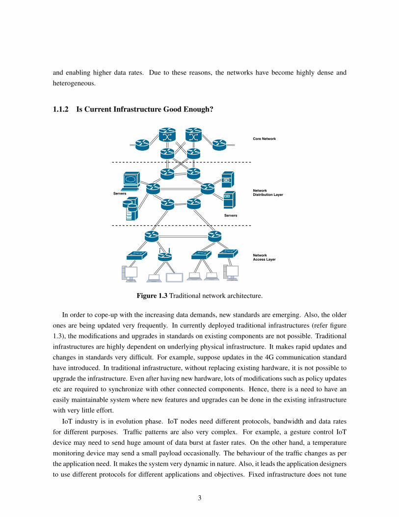
1.1.2 Is Current Infrastructure Good Enough?

Figure 1.3 Traditional network architecture.

In order to cope-up with the increasing data demands, new standards are emerging. Also, the olderones are being updated very frequently. In currently deployed traditional infrastructures (refer figure1.3), the modifications and upgrades in standards on existing components are not possible. Traditionalinfrastructures are highly dependent on underlying physical infrastructure. It makes rapid updates andchanges in standards very difficult. For example, suppose updates in the 4G communication standardhave introduced. In traditional infrastructure, without replacing existing hardware, it is not possible toupgrade the infrastructure. Even after having new hardware, lots of modifications such as policy updatesetc are required to synchronize with other connected components. Hence, there is a need to have aneasily maintainable system where new features and upgrades can be done in the existing infrastructurewith very little effort.

IoT industry is in evolution phase. IoT nodes need different protocols, bandwidth and data ratesfor different purposes. Traffic patterns are also very complex. For example, a gesture control IoTdevice may need to send huge amount of data burst at faster rates. On the other hand, a temperaturemonitoring device may send a small payload occasionally. The behaviour of the traffic changes as perthe application need. It makes the system very dynamic in nature. Also, it leads the application designersto use different protocols for different applications and objectives. Fixed infrastructure does not tune

3

itself for resource optimization in such scenarios. A system which can easily adopt and optimize itselfis needed.

Voluntarily providing the computational resources is another trend. These resources can be utilizedfor delay sensitive IoT applications, where processing data at cloud introduces unwanted communicationdelays. With fixed infrastructure, grid computing [8] based hard-coded logic can be applied for resourcemanagement. However, in IoT environment, fixed logic may not work because of dynamic behaviourof the resources. In such dynamic scenario, frequent updates in the policy and routing will be required.Hence, there is a need to have an automated system which is flexible to manage frequent updates inpolicies, rules and routes.

Use of mobile platforms is increasing day by day. Traditional networks do not handle mobility verywell. In a traditional network infrastructure, managing access points, mobility, handovers and accesscontrol is a difficult task. Hence, an architecture which supports mobility at it’s core, is required.

Majority of the fixed infrastructure solutions are proprietary and their cost is very high. It alsoeliminates the freedom of choosing different vendors for different domains and applications. Densedeployment of fixed infrastructure will be very expensive and heterogeneous deployment of such densenetwork will lack coordination. Maintaining such a system will also be very difficult and painful. Hence,an infrastructure which is economic, easily maintainable and scalable by service providers, is needed.

1.1.3 Why SDN?

Open network consortium [9] proposed a Software Defined Network (SDN) paradigm to overcomethe issues mentioned in the above section. A network build on SDN paradigm will have followingobjectives

• Any dependent entities should be minimally affected in case of system upgrades. The networkmust be maintainable.

• The network has to be adaptive. It should adapt accordingly as per changing network conditionsand user requirements.

• With dynamic user requirements or network conditions the system must scale up or down.

• The network has to be automated. Rules, policy changes and other network activities must beapplied automatically.

• The network should support user mobility.

• Network changes should be done as per network orchestration. It should support model manage-ment.

• Unlike traditional networks, where security measures are add-on features, a network should haveintegrated security.

4

Hence, a network built to achieve objectives of SDN will be able to overcome aforementioned issues.SDN does it by segregating data and control plane of the network [9]. With SDN, the concepts ofvirtualization [10] should be introduced. Without utilizing features of virtualization, it is difficult toremove the dependency on the physical hardware. With network function virtualization (NFV) [11],network elements such as router, switch, firewall, intrusion detection system etc., can be changed orconfigured without depending on underlying physical infrastructure. Features such as service functionchaining [12] and network slicing [13] can be provided using SDN and NFV techniques.

1.2 Thesis Contribution

In this thesis work, we have presented

• a self-organizing software defined infrastructure, which is capable of learning resource allocationin heterogeneous IoT environment. It minimizes the total time taken for serving all the requestsin a reliable manner.

• an economic way to allocate physical layer devices in Software Defined Wireless Network (SDWN).This work creates an opportunity for network service providers to minimize their operational ex-penditure (OpEx) with certain level of quality of service (QoS) guarantees.

• techniques to optimally allocate time in spectrum sensing. With objective of efficient allocationof sensing times in presence of special constraints, these techniques find exact solution to choose.

1.3 Thesis Outline

Chapter 2 provides an overview of SDN and SDWN. This chapter covers architecture, protocols andinteraction among various layers in software defined networking paradigm. This information will behelpful in understanding the proposed systems in later chapters.

In chapter 3, a self organizing edge computing system has been proposed. This system learns therequired parameters for allocating service requests made by IoT devices. Proposed system forwardsthe requests to network edge connected devices in such a way that the total time for all the resourcesminimizes, with certain level of reliability.

Chapter 4 proposes cost effective mechanism to allocate resources at network access layer. Thischapter formulates an optimization problem to economically allocate software defined physical layerresources in wireless networks.

Interesting cases of time optimization in spectrum sensing have been proposed in chapter 5. Thischapter presents various lemmas and proofs to find a unique solution in practical cases.

Finally, the thesis has been concluded in chapter 6 with details of future work.

5

Chapter 2

Software Defined Networks: An Overview

Due to inadequacy of traditional fixed network infrastructure for handling growing data demands,SDN is evolving. In this chapter, we will learn about SDN architecture, it’s components and variousprotocols it uses.

2.1 SDN Architecture

Figure 2.1 SDN analogy with modern computing paradigm [14].

Analogically, the evolution of SDN is same as computer systems. Refer figure 2.1 for analogicalcomparison with computer system. In early days, the proprietary computers were sold by vendors.These systems contain proprietary hardware and software owned by specific vendor. In case of systemor application extension, solutions could only be given by that specific vendor. With evolution in ar-chitecture, independent system and application software run on hardware selected by user. A user mayassemble a machine with X86 processor with Linux operating system (OS). Later, operating system canbe changed to Windows or Mac as per user requirements. Additional hardware/peripherals can also beadded. Variety of cross platform applications can be implemented in such computing environment.

6

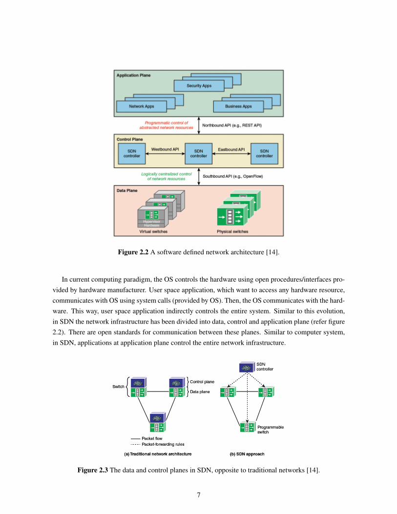
Figure 2.2 A software defined network architecture [14].

In current computing paradigm, the OS controls the hardware using open procedures/interfaces pro-vided by hardware manufacturer. User space application, which want to access any hardware resource,communicates with OS using system calls (provided by OS). Then, the OS communicates with the hard-ware. This way, user space application indirectly controls the entire system. Similar to this evolution,in SDN the network infrastructure has been divided into data, control and application plane (refer figure2.2). There are open standards for communication between these planes. Similar to computer system,in SDN, applications at application plane control the entire network infrastructure.

Figure 2.3 The data and control planes in SDN, opposite to traditional networks [14].

7

Centralized control is the major shift in SDN paradigm. In conventional network infrastructure,devices process the network traffic in a distributed manner. Each network device has its own logic forhandling the data. These devices communicate with each other and find out the most suitable path for adata flow. Contrary to this approach, in SDN, a central controller decides the path for data flow (referfigure 2.3).

Next, the data, control and application planes are presented individually. Upcoming sections provideinsight about the functionality of each plane, the protocols used and various other details.

2.2 SDN: Data Plane

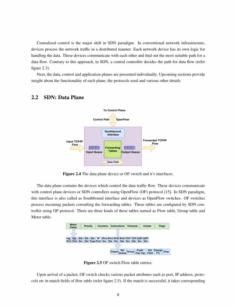
Figure 2.4 The data plane device or OF switch and it’s interfaces.

The data plane contains the devices which control the data traffic flow. These devices communicatewith control plane devices or SDN controllers using OpenFlow (OF) protocol [15]. In SDN paradigm,this interface is also called as Southbound interface and devices as OpenFlow switches. OF switchesprocess incoming packets consulting the forwarding tables. These tables are configured by SDN con-troller using OF protocol. There are three kinds of these tables named as Flow table, Group table andMeter table.

Figure 2.5 OF switch Flow table entries.

Upon arrival of a packet, OF switch checks various packet attributes such as port, IP address, proto-cols etc in match fields of flow table (refer figure 2.5). If the match is successful, it takes corresponding

8

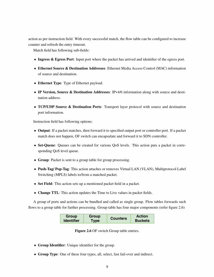
action as per instruction field. With every successful match, the flow table can be configured to increasecounter and refresh the entry timeout.

Match field has following sub-fields:

• Ingress & Egress Port: Input port where the packet has arrived and identifier of the egress port.

• Ethernet Source & Destination Addresses: Ethernet Media Access Control (MAC) informationof source and destination.

• Ethernet Type: Type of Ethernet payload.

• IP Version, Source & Destination Addresses: IPv4/6 information along with source and desti-nation address.

• TCP/UDP Source & Destination Ports: Transport layer protocol with source and destinationport information.

Instruction field has following options:

• Output: If a packet matches, then forward it to specified output port or controller port. If a packetmatch does not happen, OF switch can encapsulate and forward it to SDN controller.

• Set-Queue: Queues can be created for various QoS levels. This action puts a packet in corre-sponding QoS level queue.

• Group: Packet is sent to a group table for group processing.

• Push-Tag/ Pop-Tag: This action attaches or removes Virtual LAN (VLAN), Multiprotocol LabelSwitching (MPLS) labels to/from a matched packet.

• Set Field: This action sets up a mentioned packet field in a packet.

• Change TTL: This action updates the Time to Live values in packet fields.

A group of ports and actions can be bundled and called as single group. Flow tables forwards suchflows to a group table for further processing. Group table has four major components (refer figure 2.6)

Figure 2.6 OF switch Group table entries.

• Group Identifier: Unique identifier for the group.

• Group Type: One of these four types, all, select, fast fail-over and indirect.

9

Figure 2.7 Packet processing flow table by OF switch.

• Counters: Number of packets processed by group.

• Action Buckets: Set of actions to execute.

Figure 2.7 presents the flow chart of the packet processing by OF switch.

2.3 OpenFlow Protocol

The specifications of the message exchanges between OF switch and controller is defined by OFprotocol [16]. These specifications are advised to run over transport layer security (TLS) to have asecure channel between OF controller and switch. There are three types of messages

• Symmetric: These messages can be initiated either by OF switch or controller without otherssolicitation. The receiver always responds to the message. These messages are hello or echomessages. These messages help OF switch and controller to estimate latency, bandwidth, statusof the connected link.

• Controller to Switch: These messages are initiated by OF controller. For some special messagesresponse is required from OF switch. These messages configure flow and group tables of OFswitch. Pacaket-Out message also belongs to this category.

10

• Asynchronous: These messages are sent by OF switch to controller without it’s solicitation.These status messages are sent by OF switch when any condition switch condition such as portstatus, flow removal etc happens.

2.4 SDN: Control Plane

Northbound Interface

SDN Network

OperatingSystem (POX)

ReST APIs

To Application Plane

Southbound Interface

East

boun

d In

terf

ace

Westbound

Interface

OpenFlow

To OpenFlow Switch

To Other SDN Controller

SDNi

To Other SDN Controller

SDNi

Figure 2.8 SDN control plane interface.

Similar to functionality of operating system in computers, SDN control plane can also seen as Net-work Operating system (NOS) which maps the service requests made by application plane to OF com-plaint commands and provides information about data plane activity, topology and other statistics toapplication plane. The application plane communicates to SDN controller via northbound interface us-ing Representational State Transfer (ReST) application program interface (API). There can be multipleSDN controller in a system. These interact with each other via East/West bound interface using SDNiprotocol. As already discussed, OF switches connect to control plane via southbound interface usingOF protocol. Figure 2.8 shows all these interfaces.

Control plane provides following functionality

• Configure data plane devices as per application request.

• Managing switch topology at data plane.

• Collecting traffic statistics from OF switches.

11

• Configure shortest path for a flow at data plane.

• Manage notifications from data and application plane devices.

• Provide security mechanisms.

PoX, OpenDaylight, Beacon are a few open source implementation of SDN controllers. OpenDay-Light and Beacon are implemented in Java, while PoX is written in python. These controllers can beeasily extended to add functionality as per requirements.

2.5 SDN: Application Plane

User Interface

Data Center Networking

Mobility & Wireless

Information Centric Networking Traffic Engineering

NorthboundInterface

Measurement & Monitoring

Security & Dependebility

ReST APIs

To Control Plane

Network Service & Abstraction

Figure 2.9 SDN application plane [14].

Application plane contains applications for various tasks. These application may be used for man-aging wireless and mobile networks. Others may be used for monitoring and measurements of networktraffic. Another application may be used for enforcing QoS rules on the data plane traffic. These ap-plication use network service abstraction layer as per defined in section 3.6 of RFC7426 [17]. Networkservice abstraction layer exposes only necessary details to applications. This layer hides low level detailsof the data plane and provides high level APIs to interact with control plane.

12

Chapter 3

Self Organizing Software Defined Edge Infrastructure For IoT

Traditional IoT architectures connect the sensing devices to the Internet and send the generated datato a cloud resource for processing. This methodology works well for the applications where strict delayis not a concern. Cloud is not an ideal resource for the applications which require real time responses.This is the reason, domains such as telecommunication, health care, real time control etc. process thedata closer to the origin [18]. This computational paradigm is termed as edge computing.

Gaber et.al. [19] proposed that the edge computing needs to leverage all the resources connectedat the network edge such as laptop, tablets, desktops, smartphones etc. Although, these devices arenot always connected to the Internet, they can still be used opportunistically for various computationaltasks. Now a days, devices at the network edge such as laptops and desktop computers are being volun-tarily offered by the owners for computational purposes. Efficient utilization of all these computationalresources enhances the overall capacity of the edge system and allows it to scale. The traffic towards thecore IP network can also be reduced significantly. In this regard, we have presented a self-organizingedge infrastructure laid on the principles of SDN. We propose an intelligent software-defined EdgeController (EC) in IoT environment, which configures the infrastructure to utilize all the available re-sources efficiently for data processing. This EC learns various parameters for resource optimizationduring initial runs. After acquiring sufficient information, an integer linear programming problem forminimization of time to complete requests is formulated and solved. The solution ensures fair allocationof the requests to various resources in such a way that the total time for request completion is minimizedfor all the nodes.

The reliability of the voluntary resources is another substantial issue which is covered in this chap-ter. Many times a computational resource accepts a request, but can not process it in a timely manner.It may happen because of the battery outage, scheduling of other higher priority tasks, connection re-establishment due to mobility etc. Assigning latency sensitive tasks to such devices is a risk. The formu-lation done for minimization of time to complete requests has been extended to incorporate reliabilitymeasures. A multi-objective optimization problem is formulated and solved using Genetic Algorithm(GA). The solution to the problem provides the allocations which reliably forward the requests to theavailable resources.

13

Figure 3.1 Software defined IoT infrastructure.

Here on-wards two kind of nodes have been considered in this chapter. First kind of nodes, termedas IoT nodes, are the one which need to offload the computational tasks. These are sensing devices,which sense a physical phenomenon and transmit it to a server for further processing. In other words,IoT nodes are clients looking for servers. Second kind of nodes are termed as resources. These arethe servers which provide the APIs for computation. Using APIs provided by the resources, IoT nodesrequest for various computation tasks.

3.1 Related Work

Resource allocation in edge and participatory computing has been studied by many researchers. Inthis section, work by a few authors have been presented. Authors in [20] have presented a surveyon emerging computing technologies such as cloudlet, fog computing and mobile edge computing.Importance of code mobility is discussed in [21]. The paper has emphasized to have a new mobile cloudcomputing infrastructure in the IoT environment. The positive impact of using user-controlled edgedevices for the computation migration from the smartphone has been studied in [22]. Authors in [23]have studied the computational offloading to the edge devices such as router. Their proposed algorithmallows the efficient resource utilization. Researchers in [24] have proposed the use of cloudlets on theedge of the network to assist IoT nodes in a better way compared to the clouds. Amin et.al. [25]have presented their work on the participatory edge computing for the local community services. Intheir work, they have achieved privacy of sensed data, data analytics, resilience and real-time responseusing participatory edge computing. Resource allocation and task offloading in mobile Edge computingscenario is proposed by Tran et.al. [26]. A convex optimization technique is used for resource allocationand a heuristic algorithm has been proposed for task offloading.

14

The possibility of inclusion of SDN in Edge Computing for the mobile users is shown by Ahmet et.al.[27]. This review paper suggests the use of separate data and control planes to manage the movement ofmobile IoT devices using Cloudlets. Authors in [28] have proposed an energy efficient routing protocolusing SDN controller. They have compared the proposed routing algorithm with the standard wirelesssensor networks protocols such as Ad hoc On-Demand Distance Vector (AODV), Dynamic SourceRouting (DSR) and Destination-Sequenced Distance-Vector Routing (DSDV) on various parameterssuch as throughput, end to end delay and packet delivery ratio. Qin et.al [29] have proposed a software-defined approach to manage heterogeneous IoT and sensor devices. This is done via providing the bestmatching resource for different classes of IoT devices.

Considering the aforesaid work, we have presented a novel software defined edge computing infras-tructure, where the computational resources of the voluntary devices are utilized along with the dedi-cated edge and cloud resources. This infrastructure allocates requests via learning different parametersin software defined paradigm. The problem formulation tackles important issues such as minimizationof request completion time and reliability of all the edge resources.

3.2 Proposed System For Resource Allocation With Request Completion

Time Minimization

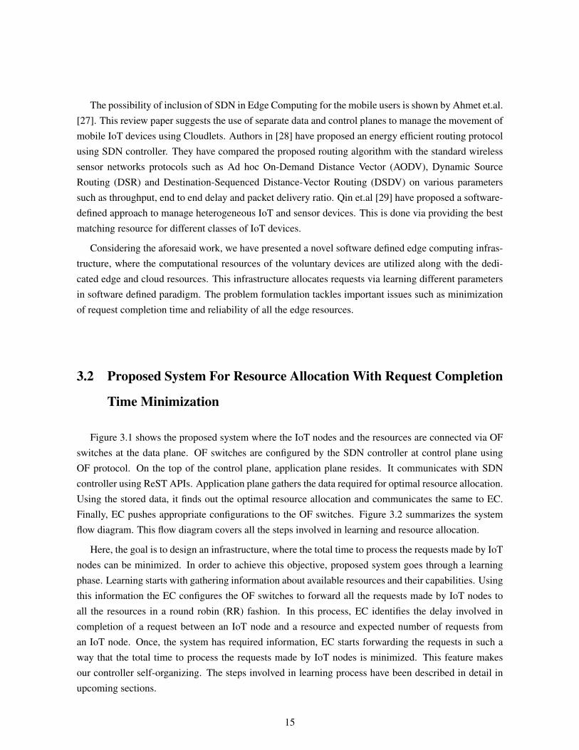
Figure 3.1 shows the proposed system where the IoT nodes and the resources are connected via OFswitches at the data plane. OF switches are configured by the SDN controller at control plane usingOF protocol. On the top of the control plane, application plane resides. It communicates with SDNcontroller using ReST APIs. Application plane gathers the data required for optimal resource allocation.Using the stored data, it finds out the optimal resource allocation and communicates the same to EC.Finally, EC pushes appropriate configurations to the OF switches. Figure 3.2 summarizes the systemflow diagram. This flow diagram covers all the steps involved in learning and resource allocation.

Here, the goal is to design an infrastructure, where the total time to process the requests made by IoTnodes can be minimized. In order to achieve this objective, proposed system goes through a learningphase. Learning starts with gathering information about available resources and their capabilities. Usingthis information the EC configures the OF switches to forward all the requests made by IoT nodes toall the resources in a round robin (RR) fashion. In this process, EC identifies the delay involved incompletion of a request between an IoT node and a resource and expected number of requests froman IoT node. Once, the system has required information, EC starts forwarding the requests in such away that the total time to process the requests made by IoT nodes is minimized. This feature makesour controller self-organizing. The steps involved in learning process have been described in detail inupcoming sections.

15

Figure 3.2 System flow summary.

3.2.1 Finding available resources

The first step towards making the system self-organized is to gather complete information about theavailable resources in the system. Before scheduling the requests, the EC must be aware of the availableresources for computation. In diverse IoT environment, different nodes may use different mechanismsand protocols for service advertisement and discovery. Nodes may use centralized or distributed ap-proaches for resource discovery. In a Constrained ReSTful Environment (CoRE) [30] the devices useCoRE link format 1 for resource discovery. Nodes can also use Resource Discovery Protocol (RDP)[31]. Both the protocols support server/client model for resource discovery. In such centralized ar-chitecture, the RDP clients (or resources) send the resource information as a well constructed queryto the RDP server and the server stores this information in a resource directory. The nodes lookingfor resources send query to RDP server and the server responds accordingly. Variety of other servicediscovery protocols in IoT setting can found in [32, 33]. It is assumed that RDP query will containmaximum capability of the resource.

The information about service mechanisms and resource databases is provided as a configurationto the proposed system. At start-up, it parses the configuration file and configures the OF based SDN

1https://tools.ietf.org/html/draft-ietf-core-resource-directory-09

16

Figure 3.3 Learning resource availability and capability.

switches in the infrastructure to capture these resource information packets about the available resources.For example, say the devices announce their capability via RDP and this information is mentionedin the configuration. The switch flow tables are configured by the edge controller to receive RDPannouncement flows on mentioned protocol and port. The edge controller parses these flows and updatesits knowledge base about available resources. If there is a RDP server in the system, EC sends the RDPquery to receive information about available resources via packet-out mechanism. It is assumed that theentire system is also connected with cloud resources and the EC has this information. Figure 3.3 depictsthe same idea.

3.2.2 Mapping resources to IoT nodes

Once EC has the list of available resources and the maximum requests they can handle, it startsforwarding requests coming from IoT nodes to available resources in a RR manner. Before doing this,EC configures the SDN switches to announce the default resource address for all the available services.IoT nodes looking for resources, receive theses notifications and start sending requests to announceddefault gateway. The EC configures the SDN switches in such a way that the requests go to all theavailable service providers one by one. For redirecting the requests to other resources, switches changethe destination address of a request from default gateway to a selected resource.

For example, a camera-equipped IoT node wants the captured images to be classified. It receives thedefault resource information and starts sending requests to the mentioned address. Due to the switchconfiguration, the destination of the request changes and the first request is forwarded to first availableimage classification service provider. The second request is forwarded to another service provider. Thisprocess goes on for subsequent requests in a RR way. With the analysis of requests and responses ECmaps the IoT nodes to the resources with various metrics such as processing delay and the number ofexpected requests from an IoT node.

17

Figure 3.4 Learning request completion time (MTTC) from IoT node to the resources.

3.2.2.1 Learning request completion time

We have already discussed that IoT environment is heterogeneous. Service providing node can beconnected via different media access protocols. They can have different processing capabilities. Theycan be static or mobile. All these situations change the time for processing a request. Via forwardingrequests to all the resources in a RR manner, our controller learns about the expected time taken for com-pleting a request. Figure 3.4 explains the idea pictorially. In order to find the lapsed time in processing arequest, EC configures the switch to send notification packets to itself as soon as a request is forwardedto a resource and resource sends the response back. Looking into the time difference, EC identifies thedelay involved. This delay is also termed as Mean Time to Complete (MTTC). This process is repeatedfor every pair of IoT node and resource.

Figure 3.5 Predicting number of expected requests from IoT nodes.

18

Figure 3.6 The resource allocation problem and the system with acquired knowledge.

3.2.2.2 Predicting number of expected requests

In the process of forwarding requests to all the available resources, the EC also determines the num-ber of expected requests from an IoT nodes in a duration. While forwarding requests in a RR manner,the EC receives the request notification (as EC configured the switches for learning MTTC, mentionedin previous subsection 3.2.2.1). The EC saves these records with a time stamp. When sufficient datais collected, application plane analyzes the data and forecasts the expected number of requests in fu-ture. Neural networks or deep learning based time series analysis techniques can be employed by theapplication plane to predict the expected number of requests in the future. Figure 3.5 explains the same.

3.2.3 Resource allocation as an optimization problem

After going through the learning phase, the system acquires the information about maximum ca-pacity of m service providing nodes represented as vector [a1, a2, . . . , am]. It also gains knowledgeabout number of expected requests from n IoT nodes, depicted as [b1, b2, . . . , bn]. It maintains a matrix[tij ] ∀ i = 1, 2, . . . ,m & j = 1, 2, . . . , n representing average time taken for completing requests of IoTnodes to service proving nodes (refer figure 3.6). xij is the number of requests forwarded to a resourcei from an IoT node j. As resource scheduling techniques based on mean time to complete are moreeffective than RR or random selection techniques [34], EC switches the allocation method from RR toMTTC (or request completion time minimization) technique via following formulation

minimizen∑

j=1

tijxij ∀ 1 ≤ i ≤ m (3.1)

subject to constraintsn∑

j=1

xij ≤ ai ∀ i = 1, 2, . . . ,m (3.2)

m∑i=1

xij = bi ∀ j = 1, 2, . . . , n (3.3)

19

xij ≥ 0 ∀ i = 1, 2, . . . ,m & j = 1, 2, . . . , n (3.4)

Equation (3.1) is the objective function. It tries to minimize the total time taken for processing therequests for all the available IoT nodes. (3.2) ensures that the requests to a service providing nodeis not more than its maximum capacity. Similarly, (3.3) divides the load from an IoT node to serviceproving nodes. (3.4) puts a lower bound on the allocations. Clearly, to have a feasible solution followingcondition must be satisfied

m∑i=1

ai >=n∑

j=1

bj (3.5)

If the above condition is not satisfied, more service providing nodes are required. The EC can requestneighbouring edge servers for more serving units or it can reserve the cloud resources to accommodaterequests. This shows the proactive behaviour of the proposed system. Solution to the above optimizationproblem provides flow allocation from IoT nodes to resources. This allocation scheme runs at user-defined intervals and application plane pushes new allocations to EC. EC changes switch configurationsaccordingly.

3.2.4 Results

The analysis of the proposed system has been done in MATLAB and mininet [35]. First, the for-mulated linear programming problem has been solved in MATLAB. Results are verified for requestcompletion time minimization and fairness. Later, a scenario is created in mininet and request comple-tion time minimization criterion is tested.

3.2.4.1 MATLAB results and analysis

The assignment problem has been solved using MATLAB function intlinprog() [36] with differentvalues of requests and processing delay (or MTTC values). The function uses dual-simplex algorithm[37] for solving the problem.

Table 3.1 MATLAB simulation parameters.Case Requests from IoT nodes Max Capacity of Resources MTTC(ms)

a 200-300 1000-2000 7-9b 200-300 1000-2000 7-17c 1000-2000 2000-4000 7-9d 1000-2000 2000-4000 7-17e 10-300 1000-2000 7-9f 280-300 1000-2000 7-9

The information about number of expected requests from IoT nodes, resource capabilities and MTTCvalues is randomly generated as per table 3.1. The table has six test cases. These cases verify the systembehaviour in different conditions such as low and high expected requests from IoT nodes, low and

20

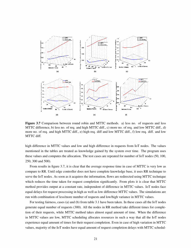
(a) (b) (c)

(d) (e) (f)

Figure 3.7 Comparison between round robin and MTTC methods. a) less no. of requests and lessMTTC difference, b) less no. of req. and high MTTC diff., c) more no. of req. and low MTTC diff., d)more no. of req. and high MTTC diff., e) high req. diff and low MTTC diff., f) low req. diff. and lowMTTC diff.

high difference in MTTC values and low and high difference in requests from IoT nodes. The valuesmentioned in the tables are treated as knowledge gained by the system over time. The program usesthese values and computes the allocation. The test cases are repeated for number of IoT nodes (50, 100,250, 300 and 500).

From results in figure 3.7, it is clear that the average response time in case of MTTC is very low ascompare to RR. Until edge controller does not have complete knowledge base, it uses RR technique toserve the IoT nodes. As soon as it acquires the information, flows are redirected using MTTC techniquewhich reduces the time taken for request completion significantly. From plots it is clear that MTTCmethod provides output at a constant rate, independent of difference in MTTC values. IoT nodes faceequal delays for request processing in high as well as low difference MTTC values. The simulations arerun with combination of less/more number of requests and low/high variance in MTTC values.

For testing fairness, cases (a) and (b) from table 3.1 have been taken. In these cases all the IoT nodesgenerate equal number of requests (300). All the nodes in RR method take different times for comple-tion of their requests, while MTTC method takes almost equal amount of time. When the differencein MTTC values are low, MTTC scheduling allocates resources in such a way that all the IoT nodesexperience equal amount of times for their request completion. Even in case of high variation in MTTCvalues, majority of the IoT nodes have equal amount of request completion delays with MTTC schedul-

21

0 20 40 60 80 100

Node Number

2100

2150

2200

2250

2300

2350

2400

2450

2500

2550

2600

To

tal T

ime S

pen

t in

th

e s

yste

m (

ms)

RR

MTTC

0 20 40 60 80 100

Node Number

2000

2500

3000

3500

4000

4500

To

tal T

ime S

pen

t in

th

e s

yste

m (

ms)

RR

MTTC

Figure 3.8 The fairness comparison. MTTC values in the left figure varies in range(7 – 9) and in range(7 – 17) in right figure.

ing. In RR allocation, the IoT nodes have different delays for both the cases. Figure 3.8 confirms thisbehaviour.

3.2.4.2 Mininet analysis

Figure 3.9 Mininet configuration. Hosts are generating requests and resources are responding.

Mininet is a network emulator in which a network can be created with virtual hosts, switches, con-trollers and links. The switches in mininet support OpenFlow. For our scenario, mininet is configuredwith four IoT nodes (h1-h4), three resources (r1-r3) and one SDN controller as per figure 3.9. The linkdelays for resources are configured to have different values. In our setup, r1, r2 and r3 are configured tohave 50ms, 200ms and 500ms of link delays respectively. It helps creating different response times fordifferent resources. A concurrent hypertext transfer protocol (HTTP) server is run on all the available

22

Table 3.2 Mininet simulation parameters.Node Link Delay(ms) Request or Response(/scenario)

h1 100 14,15,30h2 100 12,15,2h3 100 20,15,8h4 100 10,15,15r1 50 20,20,20r2 200 20,20,20r3 500 20,20,20

resources. IoT nodes run a HTTP client, which periodically sends requests to the resources as per table3.2.

First, the system looks for available resources. It captures the resource advertisement packets andknows about the maximum capacity of available resources. With this information, the SDN controllerconfigures the switch with RR mechanism and learns other required parameters. For every forwardedrequest it waits for the response and measures the MTTC values. In the simulation IoT nodes haveconfigured to send requests in a fixed interval. For simplicity, this information is communicated toEC. Table 3.2 shows all the simulation parameters. Request or Response per scenario column tells thenumber of requests sent by an IoT node (h1-h4) and maximum requests resources (r1-r3) can entertainin three scenarios. Other columns are self explanatory.

1 2 3

Scenario Numbers

0

0.002

0.004

0.006

0.008

0.01

0.012

Tota

l T

ime taken (

ms)

for

com

ple

tion

MTTC

Round Robin

Figure 3.10 Time saving in three different scenarios.

Once it has all the values, the data is fed to MATLAB to obtain allocations as per MTTC method.The allocations received from the MATLAB are given to the controller and the controller configures theswitches to allocate resources accordingly. Figure 3.10 shows that the time taken for request completion

23

by MTTC method is very less than RR method. It clearly shows that the proposed system minimizesthe delay.

Figure 3.11 Predicting resource reliability.

3.3 Proposed System For Resource Allocation With Reliability

In the previous section, the resources were allocated in such a way that the allocation is fair and totaldelay involved in processing is minimized. However, the formulation does not consider the reliabilityof the edge resources. Majority of the resources at the network edge, which are provided voluntarily,are unreliable. Highly mobile resources are prone to drop connection. These resources may refuse toentertain requests due to scheduling of high priority local tasks, connection unavailability or low batteryconditions. Hence, there is a need to update the system to incorporate resource reliability information.In this section, previously mentioned system is updated to forward the requests in such a way that totaldelay involved is minimized along with the minimization of allocated requests to the resources withhigh probability of failure.

3.3.1 Knowing resource reliability

Multiple factors can decide the reliability of a resource. Mobility, power (battery), workload, securityetc. are few such parameters. The reliability of a resource goes down in case of low battery condition.Similarly, if it is switching across access points or a user is running computational extensive applicationat the moment, it is risky to forward a request to that resource. In our study, the reliability of a resourceis termed as the number of responses sent in a timely manner for each request. As mentioned in abovesection, the EC configures the switch to find out the processing delay involved in forwarding a requestfrom IoT node to a resource. EC uses this timing in realizing reliability of a resource. If the timedifference between a request and response is more than a threshold, it is very unlikely to meet theapplication requirements. Hence, the EC reduces the reliability of such a resource or in other words it

24

Figure 3.12 Resource allocation problem and system with acquired knowledge with reliability informa-tion.

increases the probability of failure of that particular resource. Actual reliability value is calculated asthe ratio of timely sent responses (nres) to the total sent requests (nreq) i.e. nres/nreq (refer algorithm1). The same idea is depicted in figure 3.11.

Algorithm 1: Pseudo-code for calculation of resource reliability.

for each IoT request do1

Request Count = nreq + + ;2

Timestamp of incoming request = t1;3

Timestamp of outgoing request = t2;4

Processing Delay = t2 − t1;5

if Processing Delay <= Min Threshold then6

Response Count = nres + + ;7

else8/*No change in Response Count */

Reliability = nres/nreq;9

3.3.2 Resource allocation as multi-objective optimization problem

The application plane formulates a dual objective resource allocation optimization problem as perfigure 3.12. Form nodes it has probability of failure represented as [f1, f2, . . . , fm]. If xij be the numberof allocated requests to a service proving node i from an IoT node j, multi-objective optimizationproblem is formulated as following

25

minimizen∑

j=1

tijxij ∀ 1 ≤ i ≤ m

and

minimize Πmi=1f

∑nj=1 xij

i

(3.6)

subject to constraintsn∑

j=1

xij ≤ ai ∀ i = 1, 2, . . . ,m (3.7)

m∑i=1

xij = bi ∀ j = 1, 2, . . . , n (3.8)

xij ≥ 0 ∀ i = 1, 2, . . . ,m & j = 1, 2, . . . , n (3.9)

Figure 3.13 System flow summary after resource reliability information.

(3.6) is the objective function. It tries to simultaneously minimize the total time taken for processingthe requests for all the nodes and the failure probability associated with that node. Constraints are sameas before. With inclusion of resource reliability in learning steps, the updated system flow diagram lookslike figure 3.13.

26

109.996 109.998 110 110.002 110.004 110.006 110.008 110.01

Delay(f1)

9.88

9.9

9.92

9.94

9.96

9.98

10

10.02

10.04

10.06

10.08

Pro

b. o

f F

ailu

re(f

2)

×10 -201 Pareto front

Figure 3.14 Pareto front of a case.

3.3.3 Results

For solving optimization problem formulated in section 3.2.3, Genetic Algorithm [38] has been used.The problem has been coded and solved in MATLAB using function gamultiobj() [39]. The initialconfiguration parameters can be found in table 3.3. The solution of the above optimization problemgives multiple Pareto optimal solutions in terms of delay and probability of failure. The Pareto frontcan be observed in figure 3.14. To narrow down our search to achieve the appropriate optimal valuesof allocation, k-means clustering has been utilized. In this approach, the solutions are kept in threeclusters. The First cluster has values with low delay and high probability of failure. Contrary to that,the third cluster has values with high delay and low probability of failure. Unlike first and third clusters,the solutions in the second cluster are not extreme. Hence, a solution from cluster-2 is picked randomlyand the requests from IoT node to the resources are allocated accordingly.

To verify the proposed allocation strategy, the scenario as per figure 3.15, has been kept under study.N1, N2 and N3 are three data generating IoT nodes. Processing is required on the generated data.For entertaining the requests coming from IoT nodes, resources R1, R2 and R3 are available in theinfrastructure. R1 is a dedicated edge resource and it can respond to 100 requests per unit time. It isimmobile and has connectivity via Ethernet. It has redundant power and storage. Hence, the probabilityof failure is very low (.01). R3 is a cloud-connected resource. It is highly scalable and can process 500requests per unit time. The probability of R3’s failure is also very low (.01). Resource R2 is a mobilenode. It is battery powered, connected via WLAN or 4G link. When R2 is mobile, it switches acrossaccess multiple points. Hence, the reliability of R3 is lesser than R1 and R3. The probability of failurefor R2 is 0.1 and it can process 20 requests per unit time. R1 is installed close to N1 and N2. Therefore,N1 and N2 receive quick responses for the requests sent to R1. If the requests are sent to R2 or R3, the

27

Table 3.3 Initial parameters used in GA for multi-objective optimization problem.Parameter Value Details

CreationFcn @gacreationuniformInitial population is chosen with uni-form distribution.

CrossoverFcn @crossoverintermediateChildren are created using weightedaverage of parents.

CrossoverFraction 0.8 Next generation population fraction.

DistanceMeasureFcn @distancecrowding,’phenotype’Measure distance of individuals infunction space.

FunctionTolerance 10−4If relative change is less than thisvalue, the algorithm stops.

MaxGenerations 1800 Maximum iterations.

MutationFcn @mutationadaptfeasibleRandom changes in individu-als depend upon last success-ful/unsuccessful generation.

PopulationSize 200 Initial population size.

SelectionFcn @selectiontournamentParents for next generation are chosenby tournament of size 4.

time to receive the response increases. Similarly, N3 is closer to R2, so the delay involved in receivingthe responses for R1 & R3 is higher as compared to R2.

The system starts usually by collecting the available resource information. With available resourceinformation in hand, the EC configures the switches to forward the requests in a RR manner. In thelearning process the system not only learns about the mean time to complete requests and the expectednumber of requests from each IoT node but also, it keeps track of the probability of failure of a resourceusing the algorithm 1. With this information, the application plane solves the multi-objective optimiza-tion problem using GA and forwards the allocation to the EC. The EC receives the optimal allocationsfrom the application plane and configures the OF switches accordingly. For testing the formulationfollowing two conditions have been considered.

3.3.3.1 Varying probability of failure

In this case, the allocations are observed with varying probability of failure of resource R2. Asdiscussed previously, R2 is a mobile resource and it may not be able to process allocated requests ina timely manner due to conditions such as battery outage, change of access point etc. Hence, it isnecessary to understand the resource allocation changes with varying probability of failure of resourceR2. The number of expected requests from N1, N2 and N3 are 50, 100, 30 respectively. The R2’sprobability of failure is varied from 0.1 to 0.9. Figure 3.17 shows the various allocations with increasingprobability of failure of R2.

Intuitively, with the rise in probability of failure of R2, the EC should forward less number of requeststo R2. Results in figure 3.17 confirm this behaviour. With the rise in probability of failure, EC transfers

28

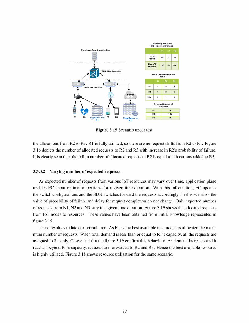
Figure 3.15 Scenario under test.

the allocations from R2 to R3. R1 is fully utilized, so there are no request shifts from R2 to R1. Figure3.16 depicts the number of allocated requests to R2 and R3 with increase in R2’s probability of failure.It is clearly seen than the fall in number of allocated requests to R2 is equal to allocations added to R3.

3.3.3.2 Varying number of expected requests

As expected number of requests from various IoT resources may vary over time, application planeupdates EC about optimal allocations for a given time duration. With this information, EC updatesthe switch configurations and the SDN switches forward the requests accordingly. In this scenario, thevalue of probability of failure and delay for request completion do not change. Only expected numberof requests from N1, N2 and N3 vary in a given time duration. Figure 3.19 shows the allocated requestsfrom IoT nodes to resources. These values have been obtained from initial knowledge represented infigure 3.15.

These results validate our formulation. As R1 is the best available resource, it is allocated the maxi-mum number of requests. When total demand is less than or equal to R1’s capacity, all the requests areassigned to R1 only. Case c and f in the figure 3.19 confirm this behaviour. As demand increases and itreaches beyond R1’s capacity, requests are forwarded to R2 and R3. Hence the best available resourceis highly utilized. Figure 3.18 shows resource utilization for the same scenario.

29

0 0.2 0.4 0.6 0.8 1

Prob. of Failure of R2

0

10

20

30

40

50

60

70

80

No

. o

f re

qu

es

ts

Resource R3

Resource R2

Figure 3.16 Probability of failure of R2 and number of allocated requests.

Figure 3.17 Number of requests allocated to an IoT node to resource with the varying reliability of R2.The probability of failure for resources R1, R2 & R3 are (a) [.01 .1 .01] (b) [.01 .3 .01] (c) [.01 .5 .01](d) [.01 .7 .01] (e) [.01 .8 .01] (f) [.01 .9 .01]

30

R1 R2 R3

Resources

0

0.2

0.4

0.6

0.8

1

% U

tilizati

on

Figure 3.18 Overall resource utilization in case of variation in number of expected requests.

Figure 3.19 Number of requests allocated to an IoT node to resource for varying expected number ofrequests. The requests made from N1, N2 & N3 for respective cases are (a) [50 100 30] (b) [20 80 40](c) [10 80 10] (d) [100 100 100] (e) [200 200 200] (f) [0 0 100]

31

Chapter 4

Economic Access Network Deployment For IoT

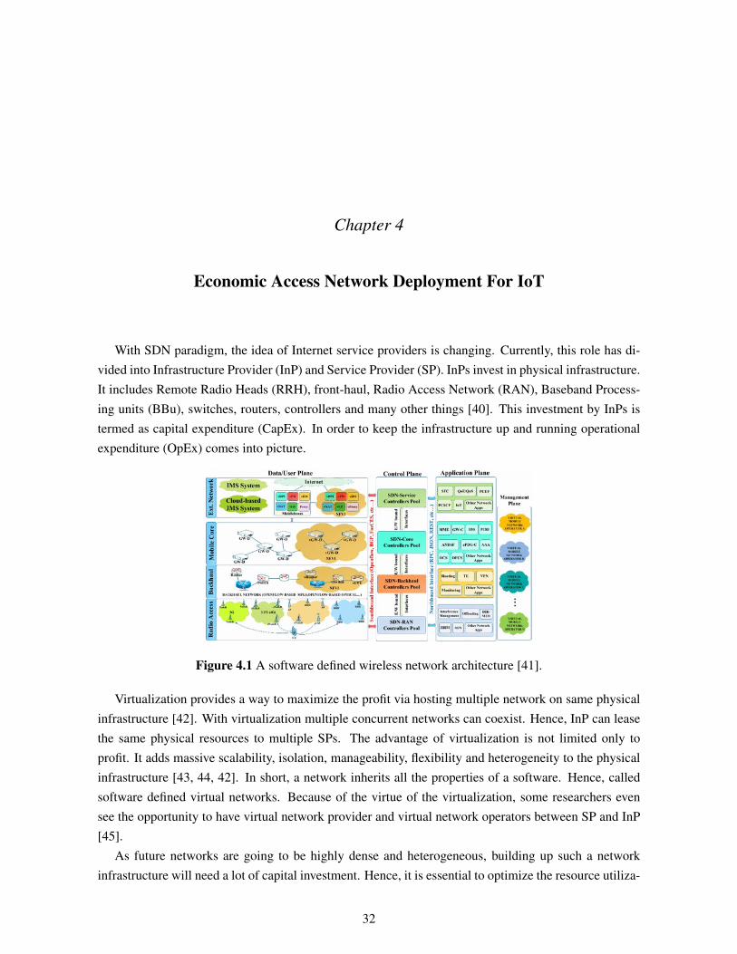
With SDN paradigm, the idea of Internet service providers is changing. Currently, this role has di-vided into Infrastructure Provider (InP) and Service Provider (SP). InPs invest in physical infrastructure.It includes Remote Radio Heads (RRH), front-haul, Radio Access Network (RAN), Baseband Process-ing units (BBu), switches, routers, controllers and many other things [40]. This investment by InPs istermed as capital expenditure (CapEx). In order to keep the infrastructure up and running operationalexpenditure (OpEx) comes into picture.

Figure 4.1 A software defined wireless network architecture [41].

Virtualization provides a way to maximize the profit via hosting multiple network on same physicalinfrastructure [42]. With virtualization multiple concurrent networks can coexist. Hence, InP can leasethe same physical resources to multiple SPs. The advantage of virtualization is not limited only toprofit. It adds massive scalability, isolation, manageability, flexibility and heterogeneity to the physicalinfrastructure [43, 44, 42]. In short, a network inherits all the properties of a software. Hence, calledsoftware defined virtual networks. Because of the virtue of the virtualization, some researchers evensee the opportunity to have virtual network provider and virtual network operators between SP and InP[45].

As future networks are going to be highly dense and heterogeneous, building up such a networkinfrastructure will need a lot of capital investment. Hence, it is essential to optimize the resource utiliza-

32

tion, maximize the network availability and minimize the operational cost with acceptable QoS param-eters. In this chapter, we formulate a node allocation problem in a SDWN using linear programmingbased on traffic forecast (refer figure 4.1). This method can be used as a service in a SDWN.

4.1 Related Work

The cost analysis for SDN based wireless infrastructure deployment is under study. Authors in [40]have presented a detailed cost modeling for setting up infrastructure in SDN/NFV based 5G networks.[46] presented the cost efficiency case study done at Finland on SDN based long term evolution(LTE)networks. Authors in [47] have modeled the cost efficiency of service function chaining (SFC) in SDNbased LTE networks. How to find a suitable service via resource discovery and allocate resources ispresented in a survey by [45]. [48] presented a model for LTE networks coupled with CapEx and OpExfor real and virtual network elements. Work by [49] showed the impact of relaying in LTE network.Authors have presented a cost model for network operator’s cost saving using relays in LTE advancednetworks. All these studies focus mostly InPs point of view. In our work, cost effective deployment ofaccess networks is presented which provides SPs perspective of cost minimization.

4.2 Proposed System Model

Our model takes inspiration from Long Term Evolution (LTE) network components. LTE networks,as shown in figure4.2, have made significant changes in conventional cellular network. In LTE, access touser equipment(UE) is provided by an enhanced NodeB (eNodeB). It is a RRH with on-site BBu or RRHconnected to a remote BBu via a front-haul. BBu can be virtualized and kept in a edge/fog computingunit. BBu connects to core network(CN) via S1 interface. CN contains other important components suchas mobility management entity (MME), home subscriber server (HSS), serving gateway (SGW) andpacket gateway (PGW). PGW connects a user to rest of the internet world via IP multimedia subsystem(IMS). The CN entities can be vitrualized and kept in cloud/fog computing unit.

In SDWN, evolved universal terrestrial radio access network (EUTRAN) and evolved packet core(EPC) units can be configured dynamically. In one time unit these can be configured to act a basestation (BS) and other time it can act as a relay of your choice (Type-1/2) [50]. If the resources requiredfor BS and relay configurations are very different. A BS need EUTRAN and EPC but a relay needsonly EUTRAN and can forward its packets to nearest BS. As all these units are configured dynamicallyin edge/fog/cloud computing units as virtualized services, the pricing also changes dynamically. FromSP’s point of view, a BS configuration is costly and a relay configuration is relatively cheap.

From above discussion it is clear that future networks would support more and more software definedcomponents and SP can take advantage of this for maximizing its profit without compromising theservice quality. In our proposed model, following steps are involved.

33

Figure 4.2 LTE network components. Shaded units can be virtualized.

1. The historical information plays important role in wireless communication. It improves overallresource utilization [51]. With this information, SP can plan the resource allocation activity inadvance and update it’s forecasting model in case of previous errors. For this reason, SP does sitesurveying and collect spatio-temporal records of the BS utilization. It collects various parametersof a BS such as peak time, off-peak time, average load etc. over a period of time. With this data itknows about the traffic behaviour at a location at a given time. Using data analysis and predictiontechniques such as time series and neural networks it can forecast the traffic at a specific BS at atime.

2. After getting expected load information, the idea is to assign high performance and costly BSto locations with heavy traffic. Locations with lower traffic with configured as relays. The highperforming BS would provide minimum processing delay and ensures certain level of QoS. Morenumber of virtualized processing units can be added on demand. This feature makes BS costly.Relays, on the other hand, forward the traffic to nearby BS for processing with less resourcerequirements. For relay there are multiple options available. SP can configure a relay as type-1/type-2, inband/outband as per the requirement.

3. Run the forecast at defined intervals and configure the nodes dynamically as per step-2.

Fig.4.3 shows its corresponding SDN architecture. Management plane (or application plane) keepstraffic statistics and runs predictive traffic analysis modules. At user defined intervals (every hour, half-hour or every few minutes), the data analysis module generate normalized expected traffic at nodes.The node allocation program takes it as input along with minimum required traffic served by BS θ

and maximum allowed distance δ. With this information it generates the allocation. Later, it maybe fed to a load balancer for BS and relay associations. Via northbound interface these allocationsare communicated to update control module. Update control module configures CN and BBu at dataplane accordingly using southbound interfaces. Monitor process at control plane monitors the status ofnetwork and provides update to management plane applications for traffic statistics.

34

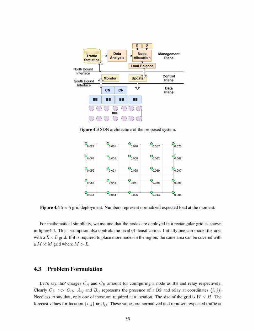
Figure 4.3 SDN architecture of the proposed system.

0.041

0.057

0.055

0.061

0.022

0.054

0.043

0.031

0.005

0.061

0.026

0.047

0.058

0.008

0.010

0.043

0.038

0.069

0.062

0.057

0.004

0.006

0.007

0.062

0.073

Figure 4.4 5× 5 grid deployment. Numbers represent normalized expected load at the moment.

For mathematical simplicity, we assume that the nodes are deployed in a rectangular grid as shownin figure4.4. This assumption also controls the level of densification. Initially one can model the areawith a L×L grid. If it is required to place more nodes in the region, the same area can be covered witha M ×M grid where M > L.

4.3 Problem Formulation

Let’s say, InP charges CA and CB amount for configuring a node as BS and relay respectively.Clearly CA >> CB . Aij and Bij represents the presence of a BS and relay at coordinates {i, j}.Needless to say that, only one of those are required at a location. The size of the grid is W ×H . Theforecast values for location {i, j} are lij . These values are normalized and represent expected traffic at

35

various nodes in the grid. Our goal is to

minimizeW∑i=1

H∑j=1

(AijCA +BijCB) (4.1)

with respect to constraints

Aij +Bij = 1 ∀ sets of {i, j} (4.2)

W∑i=1

H∑j=1

(Aijlij) ≥ θ (4.3)

0 ≤ Aij ≤ 1 ∀ sets of {i, j} (4.4)

0 ≤ Bij ≤ 1 ∀ sets of {i, j} (4.5)

Equation (4.1) is the objective function, we want to minimize. It represents the total cost incurred forplacing relay and BS at all the grid points. (4.2) places the constraint that at-least one kind of resource,either BS or relay, must be placed at the location {i, j}. This constraint maximizes the network coverage.(4.3) puts the constraint for the values obtained from forecasting. It says at-least θ population shouldbe served by BS. For example if θ is .5, then BS will be allocated in such a way that 50% of the entiretraffic is served directly by them. This constraint automatically allocates BS to nodes with higher trafficin order to minimize the cost. This happens because, for a given θ, nodes with higher traffic will be inless number.

Above mentioned constraints allocate costly BS to highly loaded nodes. Remaining nodes are con-figured as relays. A relay may forward the packet to BS via multiple hops. If there are too many hops,the delay in the system (transmission delay, queuing delay and processing delay) increases and overallQoS will degrade. Hence, there is a need to put a constraint which fixes maximum allowed hops from arelay to BS. It will ensure that in the system the nodes are allocated in such a way that relays are at-mostδ hops from BS.

W∑i=1

H∑j=1

distance (Bij −W∑i=1

H∑j=1

Aij) ≤ δ (4.6)

If constraint (4.3) is removed and constraint (4.6) is used, then there is a fixed allocation of nodes. Itdoes not vary with traffic loads.

The QoS is considered passively in the formulation. With constraint (4.6) and (4.3), minimum delayguarantees are done. Highly populated nodes are configured as BS, so there is direct communicationbetween UE and BS. Here basic processing, queuing and transmission delays are involved. When UEconnects via relay, delays associated with intermediate nodes add up. Parameter δ keeps this delayupto an acceptable level. Highly populated nodes, upto a level θ, are processed by BS. By virtue ofvirtualization and software defined features, BS maintains good QoS parameters and binding at least θpopulation efforts towards maintaining a balance with cost and acceptable QoS values.

36

θ=0.30 δ=2

0.030

0.017

0.021

0.052

0.040

0.030

0.071

0.050

0.047

0.078

0.024

0.064

0.064

0.032

0.048

0.006

0.005

0.045

0.066

0.079

0.011

0.048

0.040

0.001

0.029

θ=0.30 δ=3

0.030

0.017

0.021

0.052

0.040

0.030

0.071

0.050

0.047

0.078

0.024

0.064

0.064

0.032

0.048

0.006

0.005

0.045

0.066

0.079

0.011

0.048

0.040

0.001

0.029

θ=0.30 δ=4

0.030

0.017

0.021

0.052

0.040

0.030

0.071

0.050

0.047

0.078

0.024

0.064

0.064

0.032

0.048

0.006

0.005

0.045

0.066

0.079

0.011

0.048

0.040

0.001

0.029

θ=0.30

0.030

0.017

0.021

0.052

0.040

0.030

0.071

0.050

0.047

0.078

0.024

0.064

0.064

0.032

0.048

0.006

0.005

0.045

0.066

0.079

0.011

0.048

0.040

0.001

0.029

Figure 4.5 Node allocation with θ = 0.3 and δ = 2, 3, 4, 0 in 5 × 5 grid. Red nodes are BS and greennodes are relays.

4.4 Simulation & Results

The formulated problem is solved using intlinprog() function in MATLAB with dual-simplex algo-rithm. The allocation is tested on 5× 5 grid with various combinations of θ and δ.

If SP wants to provide the best service without considering cost, then it may allocate BS to all thenodes. In this condition, the resources in the infrastructure will not be utilized fully. This solution willalso be very expensive. In figure 4.9 this cost is shown as normal.

In figures 4.5, 4.6, 4.7 and 4.8, when only θ has taken as constraint, it is clearly visible that the BS areallocated to highly populated nodes in such a way the expected load reaches at least θ. It does not takecare of distance from the relays. Here, if a distant relay forwards the packets to BS, the delay becauseof multiple intermediate nodes would increase and overall performance of the system would degrade.To mitigate this issue δ is introduced. With usage of δ allocations change in such a way that, all the BSare at most δ distance from a relay. The simulation results in all the allocations verify this statement.

It is also seen that, when θ is kept low, less number of BS and more number of relays are deployed inthe grid. This can also be varified from the cost comparison done in figure 4.9. There is a clear trend ofincreased cost with increased θ. With minimum δ and θ the deployment cost is a little more than only θdeployments and with increased values of δ and θ the cost difference diminishes. These results suggestto use high θ and low δ parameters at peak times. At low traffic times low θ and medium δ values canbe used.

With initial observations of these results, it seems that solution automatically leads to load balancedsystem. Although detailed study is required but it seems to work with following allocations for figure4.5, where θ = 0.3 and δ = 2. There are six base stations in the grid, hence 16 to 17% traffic should beallocated to a BS. Table 4.1 shows association of relays with BS and total traffic bear by that particular

37

θ=0.50 δ=2

0.030

0.017

0.021

0.052

0.040

0.030

0.071

0.050

0.047

0.078

0.024

0.064

0.064

0.032

0.048

0.006

0.005

0.045

0.066

0.079

0.011

0.048

0.040

0.001

0.029

θ=0.50 δ=3

0.030

0.017

0.021

0.052

0.040

0.030

0.071

0.050

0.047

0.078

0.024

0.064

0.064

0.032

0.048

0.006

0.005

0.045

0.066

0.079

0.011

0.048

0.040

0.001

0.029

θ=0.50 δ=4

0.030

0.017

0.021

0.052

0.040

0.030

0.071

0.050

0.047

0.078

0.024

0.064

0.064

0.032

0.048

0.006

0.005

0.045

0.066

0.079

0.011

0.048

0.040

0.001

0.029

θ=0.50

0.030

0.017

0.021

0.052

0.040

0.030

0.071

0.050

0.047

0.078

0.024

0.064

0.064

0.032

0.048

0.006

0.005

0.045

0.066

0.079

0.011

0.048

0.040

0.001

0.029


θ=0.70 δ=2

0.030

0.017

0.021

0.052

0.040

0.030

0.071

0.050

0.047

0.078

0.024

0.064

0.064

0.032

0.048

0.006

0.005

0.045

0.066

0.079

0.011

0.048

0.040

0.001

0.029

θ=0.70 δ=3

0.030

0.017

0.021

0.052

0.040

0.030

0.071

0.050

0.047

0.078

0.024

0.064

0.064

0.032

0.048

0.006

0.005

0.045

0.066

0.079

0.011

0.048

0.040

0.001

0.029

θ=0.70 δ=4

0.030

0.017

0.021

0.052

0.040

0.030

0.071

0.050

0.047

0.078

0.024

0.064

0.064

0.032

0.048

0.006

0.005

0.045

0.066

0.079

0.011

0.048

0.040

0.001

0.029

θ=0.70

0.030

0.017

0.021

0.052

0.040

0.030

0.071

0.050

0.047

0.078

0.024

0.064

0.064

0.032

0.048

0.006

0.005

0.045

0.066

0.079

0.011

0.048

0.040

0.001

0.029


38

θ=0.90 δ=2

0.030

0.017

0.021

0.052

0.040

0.030

0.071

0.050

0.047

0.078

0.024

0.064

0.064

0.032

0.048

0.006

0.005

0.045

0.066

0.079

0.011

0.048

0.040

0.001

0.029

θ=0.90 δ=3

0.030

0.017

0.021

0.052

0.040

0.030

0.071

0.050

0.047

0.078

0.024

0.064

0.064

0.032

0.048

0.006

0.005

0.045

0.066

0.079

0.011

0.048

0.040

0.001

0.029

θ=0.90 δ=4

0.030

0.017

0.021

0.052

0.040

0.030

0.071

0.050

0.047

0.078

0.024

0.064

0.064

0.032

0.048

0.006

0.005

0.045

0.066

0.079

0.011

0.048

0.040

0.001

0.029

θ=0.90

0.030

0.017

0.021

0.052

0.040

0.030

0.071

0.050

0.047

0.078

0.024

0.064

0.064

0.032

0.048

0.006

0.005

0.045

0.066

0.079

0.011

0.048

0.040

0.001

0.029


0

50

100

150

200

Various installation conditions

To

tal C

ost

θ=

0.3

δ=

2

θ=

0.3

δ=

3

θ=

0.3

δ=

4

θ=

0.5

δ=

2

θ=

0.5

δ=

3

θ=

0.5

δ=

4

θ=

0.7

δ=

2

θ=

0.7

δ=

3

θ=

0.7

δ=

4

θ=

0.9

δ=

2

θ=

0.9

δ=

3

θ=

0.9

δ=

4

With θ+ δ

Only θ

Normal

Figure 4.9 Cost comparison of normal, threshold θ and θ + δ constraints in 5× 5 grid.

39

BS. It is clear that all the BS are loaded close to expected value. The BS selection was done usingnearest neighbour available.

Table 4.1 BS load balanced association with relays in 5× 5 grid case.BS 7 8 9 22 23 24

Relay 1,2,11 3,6,12 4,5,10,14,15 46,17 18,13,21 19,20,25Load% 15.2 15.5 15.5 17.7 18.4 17.5

40

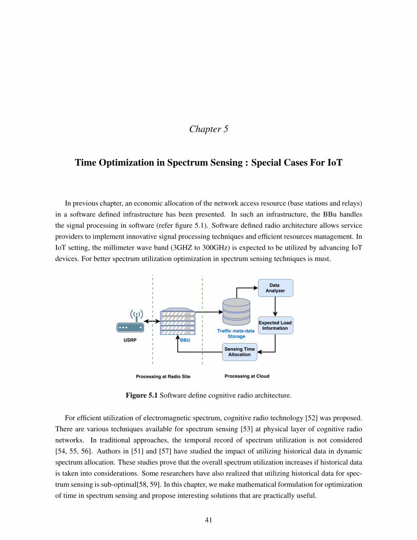
Chapter 5

Time Optimization in Spectrum Sensing : Special Cases For IoT

In previous chapter, an economic allocation of the network access resource (base stations and relays)in a software defined infrastructure has been presented. In such an infrastructure, the BBu handlesthe signal processing in software (refer figure 5.1). Software defined radio architecture allows serviceproviders to implement innovative signal processing techniques and efficient resources management. InIoT setting, the millimeter wave band (3GHZ to 300GHz) is expected to be utilized by advancing IoTdevices. For better spectrum utilization optimization in spectrum sensing techniques is must.

Figure 5.1 Software define cognitive radio architecture.

For efficient utilization of electromagnetic spectrum, cognitive radio technology [52] was proposed.There are various techniques available for spectrum sensing [53] at physical layer of cognitive radionetworks. In traditional approaches, the temporal record of spectrum utilization is not considered[54, 55, 56]. Authors in [51] and [57] have studied the impact of utilizing historical data in dynamicspectrum allocation. These studies prove that the overall spectrum utilization increases if historical datais taken into considerations. Some researchers have also realized that utilizing historical data for spec-trum sensing is sub-optimal[58, 59]. In this chapter, we make mathematical formulation for optimizationof time in spectrum sensing and propose interesting solutions that are practically useful.

41

5.1 Related Work

Authors in [55] have formulated an optimization problem in which the sensing time is optimized inorder to maximize the energy efficiency. Their main objective is to show that by optimizing the sensingtime, the energy efficiency in the spectrum sensing is improved. For wide band spectrum sensing sce-narios, authors in [56] have presented optimal sensing time and power allocation strategies under twodifferent constraints named as instantaneous and average power constraints. The authors presented away to find out such values of sensing times and power which maximizes the average throughput withconstraints of probability of detection and total transmit power. A trade-off problem on collision andthroughput have been presented in [60]. The optimization problem finds the optimal frame duration forsensing, which in turn maximizes the throughput of cognitive radio networks with an acceptable level ofcollision probability of primary user. Authors in [61] have presented a model, which utilizes the histori-cal measurements to find out the parameters such as sensing time, probability of false alarm and thresh-old for energy detection of the channel. The latest contribution in this direction is made by [54]. Theauthors have formulated a non-convex optimization problem which provides energy efficient sensingtime and power control. The authors have solved the problem keeping cross tier interference, imperfecthybrid spectrum sensing, minimum data rate requirements and energy efficiency as constraints.

Contrary to previous efforts, our work provides mathematical lemmas, proofs and examples forinteresting cases which arise in various spectrum sensing scenarios. The problem formulation is doneusing various programming techniques with justified conclusions.

5.2 Problem Formulation Using Integer Linear programming

Figure 5.2 Traditional spectrum sensing.

Consider an electromagnetic spectrum under observation has M channels labeled as 1, 2, . . . ,M .Traditional spectrum sensing methods do not take historical data into account for sensing time allocation.As depicted in fig.5.2, equal amount of time is allocated to scan all the channels. Intuitively, the channelswhich have historically large amount of data are expected to be more occupied than the channels withless amount of data. Hence, less sensing time can be allocated to highly occupied channels and moretime can be given for sensing to channels with lesser traffic.

42

5.2.1 Joint Detection-Estimation Approach to Spectrum Sensing:

Now, based on historical data, the problem of packet traffic prediction is formulated as a Linear MeanSquare Estimation (LMSE) problem. For this, the historical traffic data in different channels is takeninto account. The historical traffic data is modeled as an Auto Regressive(AR) process. In time, the unitat which the data is collected, could be an hour, day, month etc. Specifically, a pth order AR process isfit to the traffic data, i.e.

x(n+ p) = a1x(n) + a2x(n+ 1) + . . .+ apx(n+ p− 1) + w(n+ p) (5.1)

where using LMSE (i.e. Solving Yule-Walker equations) method, the coefficients are estimated and thetraffic data is predicted(on certain time unit).

Remark 1. After analyzing the gathered data, the prediction model can be chosen to be moresophisticated such as Deep neural networks.

From data analysis the predicted traffic inM channels are represented by n1, n2, . . . , nM . The trafficis normalized in following manner

qi =ni∑Mj=1 nj

∀ 1 ≤ i ≤M (5.2)

Here {q1, q2, . . . , qM} are probability mass function (PMF) values, related with traffic data of variouschannels in some time units.

Now, with expected traffic information in hand, the time optimization problem in spectrum sensingis formulated. The objective is to allocate the total time for sensing the entire band (L seconds) intotimes for sensing M channels in such a way that the average sensing time is minimized. i.e.

minimizeM∑i=1

Tiqi (5.3)

with constraintM∑i=1

Ti = L (5.4)

Remark 2. The problem formulation does not depend on the spectrum sensing approach. It can beapplied to any suitable methods such as energy detection, matched filter, cyclostationary detection etc.

Now, if no other constraints are imposed on {Ti}, then it leads to a trivial problem.

1. In this case order {qi} from smallest value to largest value, i.e. label them as {q1, q2, . . . , ˆqM} SetT1 = L, T2 = 0, . . . , TM = 0. With such a trivial allocation, T is minimized.

2. Minimum sensing time in any of the bands is lower bounded by T1(i.e smallest sensing time is at-least T1). Allocation can be as following: T1, T1, . . . , T1, (L−(M−1)T1) with (L−MT1+T1) ≥T1

43

3. Smallest sensing time is at-least T1 and other sensing times differ by at-least d time units. Allo-cation can be as following: T1, T1 + d, T1 + 2d, . . . , T1 + (M − 1)d, (L−S) with (L−S) ≥ T1,where S=(T1) + (T1 + d) + (T1 + 2d) + . . . , (T1 + (M − 1)d).

Thus realistic (practical) constraints are applied on the integer valued Ti’s.

5.2.1.1 Case A: Ti’s are in arithmetic progression (A.P.)

T1, T1 + d, . . . , T1 + (M − 1)d, must add up to total sensing time, L. Thus,

2MT1 + dM(M − 1) = 2L (5.5)

Remark 3. In above equation number of channels M and total sensing time L are known and{T1, d} are unknown variables. Since {T1, d} are always constrained to be integers, a linear Diophantineequation of form aT1 + bd = 2L appears, where a = 2M & b = M(M − 1). There are standardtechniques for solving such algebraic equations [62].

Figure 5.3 Time allocations for a)AP, b)GP case.

5.2.1.2 Case B: Ti’s are in Geometric progression (G.P.)

T1, (T1)(d), (T1)(d2), . . . , (T1)(d

M−1), must add up to total sensing time L.

T1(dM − 1)

d− 1= L (5.6)

AgainM and L are known and {T1, d} are unknowns. Hence, the following algebraic equation is solvedin integer solutions

T1dM − Ld− (T1 − L) = 0 (5.7)

To solve the above algebraic equation for {T1, d}, it is assumed that d = 2. It is required to find outT1 for T1(2M −1)−L = 0. Thus, for a givenM , T1, (2M −1) must be divisors of L. If not, no solutionexists. Suppose M is such that 2M − 1 is a prime i.e. a Mersenne prime. If L happens to be a prime

44

number, no solution exists. (It should be noted that M must necessarily be a prime for 2M − 1 to be aMersenne prime). Thus in this case for a solution to exist L must be such that its prime factorizationcontains the Mersenne prime 2M − 1. For a given M if L is divisible by 2M − 1

T1 =L

(2M − 1)(5.8)

This solution is significant in cases where energy detection is facilitated by the use of FFT of certainlength/size. Typically the FFT sizes are power of 2. Thus, d can be chosen to be a power of 2, leadingto explicit solution for T1, i.e.

T1 = Ld− 1

(dM − 1)(5.9)

Factoring L gives all the possibilities for T1. A short computation will give the desired solutions, if any.

As the probabilities decrease, the increase in sensing times assume values in an AP i.e. the rate ofincrease of sensing times is linear, or Sensing times increase geometrically (implemented by an FFT ofsuitable frequency resolution.) e.g. a, 2a, 4a, 8a, 16a, . . ..

5.2.1.3 Case C: Ti’s are in arithmetico-geometric progression (A.G.P.)

For generality, consider sensing times are in A.G.P. T1, (T1 + d)(r), (T1 + 2d)(r2), . . . , [T1 + (M −1)d](rM−1). They must add up to total sensing time L.

T1 + (T1 + d)(r) + (T1 + 2d)(r2) + . . .+ (T1 + (M − 1)d)(rM−1) = L

T1[1 + r + r2 + . . .+ rM−1] + dr[1 + 2r + 3r2 + . . .+ (M − 1)rM−2] = L

T1(1− rM )

(1− r)+ dr[

(1−MrM−1)

(1− r)+

(r − rM )

(1− r)2] = L

(5.10)

If common difference is equal to common ratio i.e d = r

T1(1− dM )

(1− d)+ d2[

(1−MdM−1)

(1− d)+

(d− dM )

(1− d)2] = L (5.11)

Thus, the Diophantine equation whose solutions are of interest are given by above equations. Solutionsmust be feasible/Non-negative integer values of {T1, d}. It can easily be reasoned that if d = 0, theabove equation reduces to (5.5) and if r = 1, (using L’Hospital’s rule) the equation reduces to (5.9).

5.3 Numerical Experiments

5.3.1 Sensing times are in A.P.

Now, let’s take a look at case A in section 5.2. For solving linear Diophantine equation 5.5, thefollowing theorem is invoked

45

Theorem 1. A solution for linear Diophantine equation ax+ by = c exists if and only if d dividesc or d|c. Here d is the greatest common divisor (G.C.D) of a & b. Also, if (x0, y0) is a solutionfor this equation, then the set of solutions of the equations consist of all integer pairs (x, y), wherex = x0 + t(b/d) and y = y0 − t(a/d) ,where t = . . . ,−2,−1, 0, 1, 2, . . .

Now the above theorem is applied and the analysis is presented via following cases:

5.3.1.1 Case 1: Only one possible solution

Suppose there are 10 channels and total sensing time is 100 ms. Hence M = 10 and L = 100 ms.Traditional approach allocates 10 ms to each channel. In our approach we place values in aT1+bd = 2L,where a = 2M, b = M(M − 1)

20T1 + 90d = 200

GCD (20, 90) = 10. (200 is divisible by 10.)

T1 = 1 + t(90/10)

d = 2− t(20/10)

(5.12)

For t = . . . .− 2,−1, 0, 1, 2, . . . there are multiple solutions but there is only one interesting solution iswith t = 0, T1 = 1 and d = 2. Therefore, our time allocation is as following (refer table 5.1)

Table 5.1 Allocation from linear diophantine equation in A.P. case.Band i ii iii iv v vi vii viii ix x

Time(ms) 1 3 5 7 9 11 13 15 17 19

Remark 4. {T1, d} must be non-negative integers.

5.3.1.2 Case 2: Multiple possible solutions

Above case only has one interesting solution for {T1, d}. What if there are multiple solutions existfor {T1, d}? Multiple solutions are possible if GCD(a, b) in aT1 + bd = 2L is a. For example if totalsensing time L is 180 ms and total no. of bands M are 9. Again in conventional solution the allocationwill be to allocate 20 ms to each band.

18T1 + 72d = 360

GCD (18, 72) = 18. (360 is divisible by 18.)

T1 + 4d = 20

One solution can be d = 5 and T1 = 0

(5.13)

T1 = 0 + t(72/18)

d = 5− t(18/18)(5.14)

46

Only for t = 1, 2, 3, 4 there are values with {T1, d} > 0. So there are multiple solutions. Sensing timescan be allocated as per table 5.2

Table 5.2 Multiple allocations from linear diophantine equation in A.P. case.Band {T1, d}↓ i ii iii iv v vi vii viii ixTime(ms) {4,4} 4 8 12 16 20 24 28 32 36Time(ms) {8,3} 8 11 14 17 20 23 26 29 32Time(ms) {12,2} 12 14 16 18 20 22 24 26 28Time(ms) {16,1} 16 17 18 19 20 21 22 23 24

5.3.2 Sensing times are in G.P.

Now consider case B in section 5.2. Suppose for scanning M = 10 bands, allocated sensing time Lis 1023 ms. With our approach, if minimum required time for sensing is T1 = 1 ms and common ratiois d = 2. After placing values in equation (5.9), allocation for each channel is as per table 5.3

Table 5.3 Single allocation in G.P. case.Band i ii iii iv v vi vii viii ix x

Time(ms) 1 2 4 8 16 32 64 128 256 512

Thus, FFT bins can be allocated for energy detection based sensing, as per above allocated time.

Now we investigate if multiple allocations for {T1, d} are possible. If total sensing time L is 21 msand number of bands M are 3, two allocations are possible (refer table 5.4). Similarly if total sensingtime L = 341 ms and number of bands M = 5, the possible allocations are as per table 5.5.

Table 5.4 Multiple allocations in G.P. case.Band {T1, d}↓ i ii iiiTime(ms) {1,4} 1 4 16Time(ms) {3,2} 3 6 12

Hence, it is clear that for some cases multiple allocations for {T1, d} are possible if the sensing timesare in G.P.

5.3.3 Sensing times are in A.G.P.

Now consider case C in section 5.2, where common difference is equal to common ratio. Supposethere are M = 3 bands, total sensing time is L = 76ms. With our approach, following times can beallocated to each channel (refer table 5.6)

It is clear that, even in A.G.P case multiple {T1, d} allocations are possible.

47

Table 5.5 Another example of multiple allocations in G.P. case.Band {T1, d}↓ i ii iii iv vTime(ms) {1,4} 1 4 16 64 256Time(ms) {11,2} 11 22 44 88 176

Table 5.6 Multiple allocations in A.G.P. case.Band {T1, d}↓ i ii iiiTime(ms) {1,3} 1 12 63Time(ms) {8,2} 8 20 48

Remark 5. The solution for {T1, d} in above cases is always a matching pair. It should also be notedthat in above cases, the real, positive solutions of diophantine equation are such that as T1 increases, ddecreases.

From above examples it is clear that, the number of solutions i.e. {T1, d} can be strictly more thanone. It is not clear which value should be picked. The appropriate solutions would be the one thatminimizes both mean and variance of sensing time random variable (defined in section 5.4).

5.4 Finding Unique Solution Using Stochastic Optimization

The software defined radios in the network gather the packet data over time for each channel andfind out the probabilities as per equation 5.2. {q1, q2, q3, . . . , qM} are such unsorted probabilities.{p1, p2, p3, . . . , pM} are sorted decreasing probabilities. In other words, the bands are ordered in se-quence from highly occupied to less occupied. If Z is spectrum sensing time random variable and Tj’sare sorted sensing time values, the mean and variance can be

Mean = E[Z] =

M∑i=1

Tiqi =∑j∈R

Tjpj (5.15)

Variance = var[Z] = E[Z2]− (E[Z])2 (5.16)

where R is a suitable index set and E[Z2] =∑

j∈R Tj2pj .

Equation 5.16 clearly shows that minimization of mean maximizes variance. We would like tominimize both mean and variance as joint optimization problem. Our aim is to arrive at a Pareto optimalsolution. Suppose qi’s are all equal. Then,

Ti = T1 , for 1 ≤ i ≤M

E[Z] =M∑j=1

Tjpj = T1(5.17)

48

5.4.1 Ti’s are in Arithmetic Progression

E[Z] =

M∑j=1

[T1 + (j − 1)d]pj

= T1(1) +M∑j=1

(j − 1)pjd

E[Z] = T1 + (µ)(d)

where µ =

M∑j=1

(j − 1)pj

(5.18)

E[Z2] =M∑j=1

(Tj)2pj

=M∑j=1

[T1 + (j − 1)d]2pj

=

M∑j=1

[T12

+ (j − 1)2d2 + 2(j − 1)T1d]pj

= T12

+ d2M∑j=1

(j − 1)2pj + 2T1dM∑j=1

(j − 1)pj

= T12

+ (α)d2 + (2T1d)(µ)

where α =M∑j=1

(j − 1)2pj

(5.19)

var[Z] = T12

+ (α)d2 + (2T1d)µ− (T12

+ µ2d2 + 2µT1d)

= (α)(d2)− µ2d2

= (α− µ2)d2(5.20)

Optimal choices of {T1, d} are coupled. Thus, issue comes down to minimize E[Z] as well as var[Z].Again, we need to select T1 and d from possibly non-unique solutions for {T1, d} determined by Dio-phantine equation. T1 only affects E[Z]. It does not effect var[Z]. So T1 should be chosen as small aspossible.

5.4.1.1 Mean Sensing Time Minimization Only

First, let’s take the case where only mean sensing time minimization is required. As per section5.3.1.2, we get multiple choices for {T1, d}. {(a1, d1), . . . , (al, dl), . . . , (aK , dK)}, are such solutions

49

and the values are positive and real integers. If a1 < · · · < al < · · · < aK , then d1 > · · · > dl > · · · >dK .

Lemma 1. (a1, d1) is the best solution which minimizes the expected value E[Z]

Proof 1. For proving (a1, d1) gives minimum E[Z], we prove that

al + µdl ≥ a1 + µd1 for l = 2, 3, . . . ,K (5.21)

i.e. al − a1 ≥ µ(d1 − dl) for l = 2, 3, . . . ,K

i.e.al − a1d1 − dl

≥ µ for l = 2, 3, . . . ,K (5.22)

Now, (a1, d1) and (al, dl) both satisfy the Linear Diophantine equation (5.5). Therefore, we can

write

M × a1 +(M − 1)M

2× d1 = L (5.23)

M × a1 = L− (M − 1)M

2× d1

M × al +(M − 1)M

2× dl = L (5.24)

M × al = L− (M − 1)M

2× dl

Multiplying (5.22) by M on both sides, we get

M × al − a1d1 − dl

≥M × µ (5.25)

M × al −M × a1d1 − dl

≥M × µ (5.26)[L− (M−1)M

2 × dl]−[L− (M−1)M

2 × d1]

(d1 − dl)≥M × µ (5.27)

(M−1)M2 × (d1 − dl)

(d1 − dl)≥M × µ (5.28)

(M − 1)

2≥ µ (5.29)

Substituting the value of µ, we get

(M − 1)

2≥

M∑j=1

(j − 1)pj (5.30)

If above expression is proved, then (a1, d1) is the best solution, which minimizes E[Z]. The detailedproof is in the appendix A Q.E.D.

50

5.4.1.2 Simultaneous Mean and Variance Minimization

For minimizing E[Z] and var[Z] simultaneously with respect to d (treating T1 as constant.)

E[Z] = f(d) = T1 + (µ)(d)

var[Z] = (α− µ2)d2

hence(α− µ2) ≥ 0

(5.31)

Lemma 2. At E[Z] = var[Z] unique optimal solution for d exists.

Proof: For an optimal solution

E[Z] = var[Z]

T1 + (µ)(d) = (α− µ2)d2

(α− µ2)d2 − µd− T1 = 0

ad2 + bd+ c = 0

where a = (α− µ2), b = −µ, c = −T1

(5.32)

b2 − 4ac > 0 for d to be real.

µ2 − 4(α− µ2)(−T1) > 0

µ2 + 4(α− µ2)T1 > 0 since (α− µ2) > 0

(5.33)

The zeros are distinct, thus we are interested in the value of d in the first quadrant. Hence, a uniqueoptimal solution for d is achieved. Q.E.D. Note that for optimal solution closest integer value of d isutilized.

Remark 6. We expect that the similar kind of optimization problem formulated in the time optimalspectrum sensing to arise in other applications. The above lemma provides solution.

51

5.4.2 Ti’s are in Geometric Progression

E[Z] =M∑j=1

Tjpj

E[Z] =

M∑j=1

(T1dj−1)pj

= T1(M∑j=1

dj−1pj)

E[Z2] =M∑j=1

(Tj)2pj

=M∑j=1

(T12d2(j−1))pj

var[Z] = E[Z2]− (E[Z])2

= T12[M∑j=1

d2j−2pj ]− T12[M∑j=1

djpj ]2

= T12[(

M∑j=1

d2j−2pj)− (

M∑j=1

djpj)2]

(5.34)

Let’s

E[Z] = T1f(d)

var[z] = T12R(d)

(5.35)

where f(d) =M∑j=1

dj−1pj and

R(d) = (

M∑j=1

d2j−2pj)− (

M∑j=1

djpj)2

= f(d2)− [f(d)]2

5.4.2.1 Mean Sensing time minimization only

First consider the case when only mean sensing time minimization is required. After solving GPcase in section 5.3, we get multiple solutions as {(a1, d1) . . . (al, dl) . . . (aK , dK)}, which are positiveand real integers. If a1 < · · · < al < · · · < aK , then d1 > · · · > dl > · · · > dK .

Lemma 3. (a1, d1) is the best solution which minimizes the expected value E[Z].

52

Proof 2.

al

M∑j=1

dj−1l pj ≥ a1M∑j=1

dj−11 pj for l = 2, 3, . . . ,K (5.36)

al(p1 + dlp2 + d2l p3 + . . .+ dM−1l pM ) ≥ a1(p1 + d1p2 + . . .+ dM−11 pM )

Moving terms related to pM to RHS

p1(al − a1) + p2(aldl − a1d1) + p3(ald2l − a1d21) + . . . ≥ pM (ald

M−1l − a1dM−11 ) (5.37)

Now, we know that sum of series generated by both (a1, d1) and (al, dl) for l = 2, 3, . . . ,K is equal.

al + aldl + ald2l + . . .+ ald

M−1l = a1 + a1d1 + . . .+ a1d

M−11 (5.38)

Rearranging terms

(al − a1) + (aldl − a1d1) + (ald2l − a1d21) + . . . = (a1d

M−11 − aldM−1l )

Comparing the above result with (5.37), it is clear that if p1 = p2 = . . . = pM , LHS is equal to

RHS. Again the probability values are decreasing p1 > p2 > . . . > pM , so (5.37) reduces to proof if

c1 + c2 + c3 + . . .+ cM−1 = cM where ci’s are positive constants, then

p1c1 + p2c2 + p3c3 + . . .+ pM−1cM−1 > pMcM (5.39)

Replacing cM = c1 + c2 + c3 + . . .+ cM−1

p1c1 + p2c2 + p3c3 + . . .+ pM−1cM−1 > pM (c1 + c2 + c3 + . . .+ cM−1)

c1(p1 − pM ) + c2(p2 − pM ) + c3(p3 − pM ) + . . .+ cM−1(pM−1 − pM ) > 0

As ci’s are positive and p1 > p2 > . . . > pM LHS is a positive quantity. Hence (5.39) holds true and(5.36) holds true as well. Q.E.D.

5.4.2.2 Simultaneous Mean and Variance Minimization

The optimal choice of minimal T1 will be optimal for both E[Z] and var[Z]. But as we discussedearlier, minimization of E[Z] with respect to d will maximize var[z]. Thus we are interested in Paretooptimal solution. It provides jointly optimal choices for d with minimized E[Z] and var[z]. We nowprove that if f(d) is minimized, R(d) is maximized. If f(t) is minimized, then f(t2) is maximized.

53

Suppose we consider the unconstrained optimization/minimization of f(t) then

Let K(t) = t2 ⇒ f(t2) = f(K(t))

df(K(t))

dt=df

dk

dk

dt= (

df

dt)(2t)

d2f(K(t))

dt2=d2f

dt2(2t) + (

df

dt)(2)

df(K(t))

dt= 0 if and only if

df

dt= 0

(5.40)

Further, the minima of f(.) are in the left half plane. Suppose they are real valued, e.g. to

d2f

dt2|t=t0 > 0 with t0 < 0

d2f(K(t))

dt2|t=t0 =

d2f

dt2(2t)|t=t0 + 0

Since t < t0

d2f(K(t))

dt2|t=t0 < 0

(5.41)

f(t2) is maximized, when f(t) is minimized. Thus, we look for Pareto optimal solution for d i.e.denoted t here. So use closest solution of (5.6) pair of T1, d to Pareto optimal solution.

Pareto Optimal Solution: (Fixed Point Equation)

E[Z] = T1f(d)

E[Z2] = T12g(d)

E[Z] = var[Z]

note that g(d) = f(d2)

T1f(d) = T12g(d)− T1

2(f(d))2

T1f(d2)− T1(f(d))2 − f(d) = 0

(5.42)

Since f(d) is a polynomial in d, we have a polynomial equation which has multiple zeros. To determineoptimal d, choose smallest real d that is feasible. Let M=3,

f(d) =3∑

j=1

d(j−1)pj = p1 + dp2 + d2p3

g(d) = f(d2) =

3∑j=1

d2j−2pj = p1 + d2p2 + d4p3

(5.43)

Replace values in equationT1f(d2)− T1(f(d))2 − f(d) = 0 (5.44)

Let T1 = 1, p1 = .5, p2 = .3, p3 = .2

(p1 + d2p2 + d4p3)− (p1 + dp2 + d2p3)2 − (p1 + dp2 + d2p3) = 0

54

50 100 150 200 250

Total Sensing Time

0

5

10

15

20

25

30

35

40

Mea

n s

ensi

ng

tim

e in

to

sca

n a

ch

ann

el (

ms)

Our Approach

Traditional Approach

0 5 10 15 20 25

Number of Channels to scan

0

2

4

6

8

10

12

14

16

18

20

Mea

n s

ensi

ng

tim

e in

to

sca

n a

ch

ann

el (

ms)

Our Approach

Traditional Approach

Figure 5.4 Comparison of mean sensing times. Left figure is run with fixed number of channel (M =5) and varying total scanning times (L = [100, 150, 200] ms). Figure in right is run with fixed totalscanning time (L = 100ms) and varying number of channels (M = [5, 10, 20]).

After solving equations values for d = 2.43, -1.26, -0.20±0.68i

In the above example, the solution contains only one positive real value that is of our interest. Restof the values are not useful. Take the closest integer value of d which is real positive optimal solution.

Summary: We now have a summary of approaches to find optimal sensing times in various channels.

1. Based on data, predict the Probabilities related to spectrum band occupancy.

2. Allocate Sensing Times in the order of probability values i.e. if a band is highly occupied (prob-abilistic), allocate smaller sensing time and vice-versa.

3. Assume that the sensing times are in A.P./G.P. Compute solution to the integer programmingproblem (or the Diophantine equation.) If there is more than one solution, we need to decide thesolution that must be chosen.

4. Find solution/solutions which minimize the mean, variance (assuming that the sensing time valuesare in A.P./G.P.) and find unique/multiple solutions.

5.5 Results

Now, we validate the lemmas with numerical examples.

5.5.1 Sensing times are in A.P.

First, the total sensing time for a band is fixed and number of channels are varied. In second case,number of channels are fixed and total sensing time for channels is varied. Then, mean sensing timeusing our optimization technique is compared with traditional spectrum sensing. Figure 5.5.1 shows thecomparison for both the cases.

55

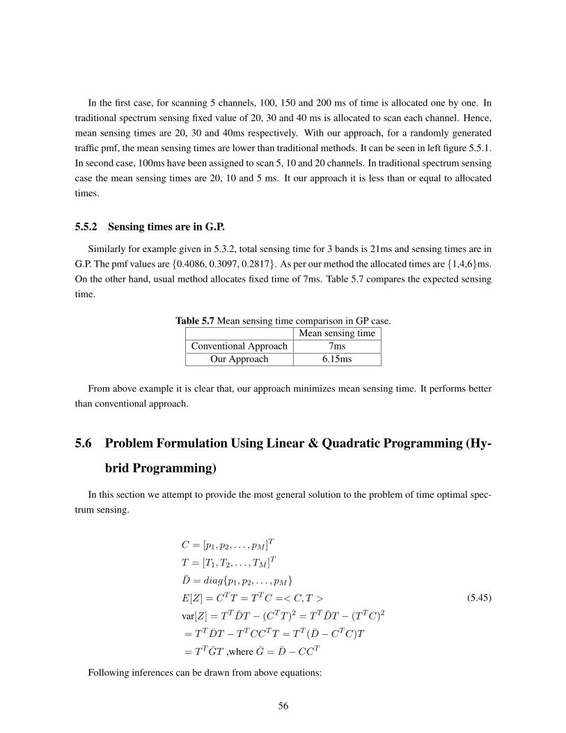
In the first case, for scanning 5 channels, 100, 150 and 200 ms of time is allocated one by one. Intraditional spectrum sensing fixed value of 20, 30 and 40 ms is allocated to scan each channel. Hence,mean sensing times are 20, 30 and 40ms respectively. With our approach, for a randomly generatedtraffic pmf, the mean sensing times are lower than traditional methods. It can be seen in left figure 5.5.1.In second case, 100ms have been assigned to scan 5, 10 and 20 channels. In traditional spectrum sensingcase the mean sensing times are 20, 10 and 5 ms. It our approach it is less than or equal to allocatedtimes.

5.5.2 Sensing times are in G.P.

Similarly for example given in 5.3.2, total sensing time for 3 bands is 21ms and sensing times are inG.P. The pmf values are {0.4086, 0.3097, 0.2817}. As per our method the allocated times are {1,4,6}ms.On the other hand, usual method allocates fixed time of 7ms. Table 5.7 compares the expected sensingtime.

Table 5.7 Mean sensing time comparison in GP case.Mean sensing time

Conventional Approach 7msOur Approach 6.15ms

From above example it is clear that, our approach minimizes mean sensing time. It performs betterthan conventional approach.

5.6 Problem Formulation Using Linear & Quadratic Programming (Hy-

brid Programming)

In this section we attempt to provide the most general solution to the problem of time optimal spec-trum sensing.

C = [p1, p2, . . . , pM ]T

T = [T1, T2, . . . , TM ]T

D = diag{p1, p2, . . . , pM}

E[Z] = CTT = T TC =< C, T >

var[Z] = T T DT − (CTT )2 = T T DT − (T TC)2

= T T DT − T TCCTT = T T (D − CTC)T

= T T GT ,where G = D − CCT

(5.45)

Following inferences can be drawn from above equations:

56

• G is a laplacian like matrix in the sense that the diagonal elements are positive and off diagonalelements are negative. Further, the sum of rows is zero just like laplacian matrix in graph theory.It is positive semi-definite.

• -G is a symmetric generator matrix.

Example:

G = D − CCT

G =

p1 0 0

0 p2 0

0 0 p3

− p1

2 p1p2 p1p3

p1p2 p22 p2p3

p1p3 p2p3 p32

=

p1(1− p1) −p1p2 −p1p3−p1p2 p2(1− p2) −p2p3−p1p3 −p2p3 p3(1− p3)

(5.46)

Our goal is to arrive at non-trivial T vector which minimizes the variance of random variable Z.Function of interest for arriving at solutions where E[Z] = var[Z]:

J(T ) = var[Z]− E[Z]

= T T GT − T TC

=[T T 1

] [ G 0

−CT 0

][T

1

] (5.47)

We investigate the structure of matrix G before providing a solution to the problems proposed above.

Remark 7. Ge = 0 where e =[1 1 . . . 1

]TG = GT

We use Laplacian and Laplacian like matrix interchangeably.

5.6.1 Most General Problem Solution

We now consider the problem of minimization of E[Z] as well as var[Z] of the random variable Z.In most general case Ti’s constitutes the integer components of a partition of the total sensing time, Li.e.

M∑i=1

Ti = L (5.48)

This constitutes the most general constraint without imposing any other constraint on Ti’s.

57

We now reason that the quadratic programming associated with minimization of var[z] can be re-duced to M linear programming problems.From above discussion

var[Z] = T T GT

By cholesky decomposition

G = NNT

T T GT = T T NNTT

= (T T N)(NT T )

= Y T Y , where Y = NT T

=M∑i=1

yi2

(5.49)

Minimizing var[z], reduces to minimizing yi for 1 ≤ i ≤ M . But Y is a linear objective function in T .Thus, minimization of var[Z] amounts to solving M linear programming problems.

In nutshell, our optimization problem reduces to solving M + 1 integer linear programming problem(including minimization of mean) i.e. E[Z] = T T C subject to the constraint in (5.48).

Remark 8. Without imposing any other constraint on Ti’s, we are led to trivial solution(as discussedearlier) in optimizing mean and variance of sensing time random variable. Thus, realistic constraint areimposed in the multi-linear objective optimization problem to get interesting solutions.

5.6.2 Properties of laplacian type matrix arising in variance expression of a Discrete

Random Variable Z:

Can (linear algebraic) properties of matrix G be capitalized to derive new results on variance mini-mization? To study properties of laplacian like matrix G = D−CCT where D = diag{p1, p2, . . . , pM},C = [p1, p2, . . . , pM ]T , G = GT

1. Eigen values are all real.

2. G is positive semidefinite, with an eigen value at zero (e . . . all ones vector). e is in the null spaceof G.

3. 0 is the smallest eigen value and all other eigen values lie on real axis.

4. Bounds on spectral radius of G

n∑j=1

Gij =

n∑j=1

Dij − pj∑

(p1 + . . .+ pj−1 + pj + . . .+ pM )

= pj − pj = 0 (5.50)

58

n∑j=1

|Gij | = pj(1− pj) + |pj(p1 + . . .+ pj−1 + pj+1 + . . .+ pM )|

= pj(1− pj) + |pj(1− pj)|

= 2pj(1− pj)(5.51)

From linear algebra, we have that

minj{2pj(1− pj)} ≤ Spectral radius(G) ≤ max

j{2pj(1− pj)}

All eigen values of G lie in the interval [0,1).

59

Chapter 6

Conclusions

Three areas of resource allocation and optimization in a software defined IoT infrastructure have beenpresented in this thesis work. In first part, optimization of computation resources at the network accesslayer has been presented. This section focuses on forwarding the requests originated from various IoTnodes to resources for processing in such a way that the total time to complete the requests is minimizedwith certain level of reliability. To achieve this objective, first the system learns the required parametersand then applies it for optimal allocation. The simulation results confirm that the system forwardsthe IoT requests to available resources with objectives of minimization of delay involved in requestcompletion and improved reliability.

In second part covered dynamic configuration of devices at the network access layer. In this effortthe devices have been configured dynamically, as per expected traffic load. In an IoT infrastructure,this method can help network service providers to minimize their operational cost with certain level ofquality of service guarantees.

Third part focused on optimization of spectrum sensing time in IoT environment. In this part, thetime to scan various channels is obtained using historical traffic on that channel. Optimization problemhas been formulated considering the allocations are in arithmetic, geometric and arithmetic-geometricprogression. In these special cases multiple solutions are possible. The exact solution was chosen usingstochastic programming model.

Our system learns various parameters by forwarding information over southbound interfaces usingOF. Hence, study on control flow overhead is required. The sensing model is expected to be embedwith detection theory, where results in terms of probability of missed detection and false alarm can bepresented. The proposed methods can be used as a software as a service in SDN environment. A serviceprovider can utilize these services by following the design considerations mentioned in the proposedsystem. This work opens new ways to encourage monetization in the edge system. Economic models toreward voluntary devices can be created.

60

Appendix A

Consider a discrete lattice random variable Z, assuming values {1, 2, . . . ,M} with probabilities{p1, p2, . . . , pM}. Here p1 + p2 + . . .+ pM = 1 and p1 > p2 > . . . > pM . We prove that

(M − 1)

2

=∑M

j=1 (j − 1)pj iff p1 = p2 = . . . = pM

>∑M

j=1 (j − 1)pj if p1 > p2 > . . . > pM(A.1)

Proof 3. We prove the result by mathematical induction. Let M = 2. Let p1 = 12 + ε, p2 = 1

2 − ε,

where ε > 0. Solving RHS2∑

j=1

(j − 1)pj = p2 =1

2− ε

Above equation is equal to LHS if and only if ε = 0 for other values of ε LHS > RHS.

Now let M = 3. Let p1 = 13 + ε1, p2 = 1

3 + ε2 and p3 = 13 + ε3, where ε1 + ε2 + ε3 = 0 and

ε1 > ε2 > ε3. Solving RHS3∑

j=1

(j − 1)pj = p2 + 2p3

= (1

3+ ε2) + 2(

1

3+ ε3)

= 1 + ε2 + 2ε3 = 1− 2ε1 − ε2

Above equation is equal to LHS if and only if −2ε1− ε2 = 0 for other values of ε1 and ε2 LHS > RHS.

Claim is true for M = k.Now let M = k + 1 and pk+1 = 1k+1 − ε where ε > 0. Solving RHS

k+1∑j=1

(j − 1)pj = p2 + 2p3 + . . .+ kpk+1

= (

k∑i=1

pi)(p2∑ki=1 pi

+ 2p3∑ki=1 pi

+ . . .+ (k − 1)pk∑ki=1 pi

) + kpk+1 (A.2)

61

As p1 + p2 + . . . + pk+1 = 1. Therefore∑k

i=1 pi = 1 − pk+1 and for M = k, p2∑ki=1 pi

+ 2 p3∑ki=1 pi

+

. . .+ (k − 1) pk∑ki=1 pi

= (k−1)2 . Keeping values in equation (A.2)

= (1− pk+1)((k − 1)

2) + kpk+1

= (1− 1

k + 1+ ε)(

(k − 1)

2) + k

1

k + 1− kε

=k

2− ε(k + 1)

2(A.3)

Above equation is equal to LHS if and only if ε = 0 for other values of ε LHS > RHS. Hence (A.1)holds true. Q.E.D.

62

Related Publications

1. Rhishi Pratap Singh, Jitender Grover and Rama Murthy Garimella, “Self Organizing SoftwareDefined Edge Controller in IoT Infrastructure,” 1st International Conference on Internet of Thingsand Machine Learning (IML), UK, October 2017.

2. Rama Murthy Garimella and Rhishi Pratap Singh, “Time Optimization in Spectrum Sensing:Interesting Cases,” 6th IEEE International Conference on Reliability, Infocom Technologies andOptimization (ICRITO), India, September 2017.

3. Rhishi Pratap Singh and Rama Murthy Garimella, “Economic Node Allocation in Software De-fined Wireless Networks with Forecasted Traffic and Distance Constraints,” 8th IEEE Interna-tional Conference on Computing Communication and Networking Technologies (ICCCNT), In-dia, July 2017.

63

Bibliography

[1] “Cisco visual networking index: Forecast and methodology, 2016–2021,” White Paper, Cisco, Feb.2016.

[2] “The zettabyte era: Trends and analysis,” White Paper, Cisco, June 2016.

[3] “Cisco visual networking index: Global mobile data traffic forecast update, 2016–2021,” WhitePaper, Cisco, Feb. 2016.

[4] A. Saeed, M. Ammar, K. A. Harras, and E. Zegura, “Vision: The Case for Symbiosis inthe Internet of Things,” in Proceedings of the 6th International Workshop on Mobile CloudComputing and Services, ser. MCS ’15. New York, NY, USA: ACM, 2015, pp. 23–27. [Online].Available: http://doi.acm.org/10.1145/2802130.2802133

[5] B. Yin, W. Shen, L. X. Cai, and Y. Cheng, “A Mobile Cloud Computing Middleware forLow Latency Offloading of Big Data,” in Proceedings of the 2015 Workshop on Mobile BigData, ser. Mobidata ’15. New York, NY, USA: ACM, 2015, pp. 31–35. [Online]. Available:http://doi.acm.org/10.1145/2757384.2757390

[6] A. V. Dastjerdi and R. Buyya, “Fog computing: Helping the Internet of Things realize its poten-tial,” Computer, vol. 49, no. 8, pp. 112–116, 2016.

[7] M. Satyanarayanan, P. Simoens, Y. Xiao, P. Pillai, Z. Chen, K. Ha, W. Hu, and B. Amos, “Edgeanalytics in the internet of things,” IEEE Pervasive Computing, vol. 14, no. 2, pp. 24–31, 2015.

[8] I. Foster, Y. Zhao, I. Raicu, and S. Lu, “Cloud computing and grid computing 360-degree com-pared,” in Grid Computing Environments Workshop, 2008. GCE’08. Ieee, 2008, pp. 1–10.

[9] “Software-Defined Networking (SDN) Definition - Open Networking Foundation,” jun 2017.

[10] Sdx Central, “What is NFV Network Functions Virtualization Definition?”https://www.sdxcentral.com/nfv/definitions/whats-network-functions-virtualization-nfv/.

[11] B. Han, V. Gopalakrishnan, L. Ji, and S. Lee, “Network function virtualization: Challenges andopportunities for innovations,” IEEE Communications Magazine, vol. 53, no. 2, pp. 90–97, 2015.

64

[12] W. John, K. Pentikousis, G. Agapiou, E. Jacob, M. Kind, A. Manzalini, F. Risso, D. Staessens,R. Steinert, and C. Meirosu, “Research directions in network service chaining,” in Future Networksand Services (SDN4FNS), 2013 IEEE SDN for. IEEE, 2013, pp. 1–7.

[13] J. Ordonez-Lucena, P. Ameigeiras, D. Lopez, J. J. Ramos-Munoz, J. Lorca, and J. Folgueira,“Network Slicing for 5G with SDN/NFV: Concepts, Architectures, and Challenges,” IEEE Com-munications Magazine, vol. 55, no. 5, pp. 80–87, 2017.

[14] W. Stallings, Foundations of modern networking: SDN, NFV, QoE, IoT, and Cloud. Addison-Wesley Professional, 2015.

[15] The Open Networking Foundation, “OpenFlow Switch Specification,” Jun. 2012.

[16] N. McKeown, T. Anderson, H. Balakrishnan, G. Parulkar, L. Peterson, J. Rexford,S. Shenker, and J. Turner, “OpenFlow: Enabling Innovation in Campus Networks,” SIGCOMMComput. Commun. Rev., vol. 38, no. 2, pp. 69–74, Mar. 2008. [Online]. Available:http://doi.acm.org/10.1145/1355734.1355746

[17] E. Haleplidis, K. Pentikousis, J. DENAZIS, et al., “SDN: Layers and Architecture Terminology,”Internet Requests for Comments, RFC Editor, RFC 7426, January 2015. [Online]. Available:https://tools.ietf.org/rfc/rfc6690.txt

[18] W. Shi, J. Cao, Q. Zhang, Y. Li, and L. Xu, “Edge computing: Vision and challenges,” IEEEInternet of Things Journal, vol. 3, no. 5, pp. 637–646, 2016.

[19] M. M. Gaber, J. B. Gomes, and F. Stahl, “Pocket data mining,” Big Data on Small Devices. Series:Studies in Big Data, 2014.

[20] Y. Ai, M. Peng, and K. Zhang, “Edge cloud computing technologies for internet of things: Aprimer,” Digital Communications and Networks, 2017.

[21] P. Patil, A. Hakiri, and A. Gokhale, “Cyber foraging and offloading framework for internet ofthings,” in Computer Software and Applications Conference (COMPSAC), 2016 IEEE 40th An-nual, vol. 1. IEEE, 2016, pp. 359–368.

[22] A. Bhattcharya and P. De, “Computation offloading from mobile devices: Can edge devices per-form better than the cloud?” in Proceedings of the Third International Workshop on AdaptiveResource Management and Scheduling for Cloud Computing. ACM, 2016, pp. 1–6.

[23] F. Samie, V. Tsoutsouras, L. Bauer, S. Xydis, D. Soudris, and J. Henkel, “Computation offloadingand resource allocation for low-power IoT edge devices,” in Internet of Things (WF-IoT), 2016IEEE 3rd World Forum on. IEEE, 2016, pp. 7–12.

[24] M. Satyanarayanan, “The emergence of edge computing,” Computer, vol. 50, no. 1, pp. 30–39,2017.

65

[25] A. M. Khan and F. Freitag, “On Participatory Service Provision at the Network Edge with Com-munity Home Gateways,” Procedia Computer Science, vol. 109, pp. 311–318, 2017.

[26] T. X. Tran and D. Pompili, “Joint Task Offloading and Resource Allocation for Multi-ServerMobile-Edge Computing Networks,” arXiv preprint arXiv:1705.00704, 2017.

[27] A. C. Baktir, A. Ozgovde, and C. Ersoy, “How Can Edge Computing Benefit from Software-Defined Networking: A Survey, Use Cases & Future Directions,” IEEE Communications Surveys& Tutorials, 2017.

[28] C. Kharkongor, T. Chithralekha, and R. Varghese, “A SDN Controller with Energy Efficient Rout-ing in the Internet of Things (IoT),” Procedia Computer Science, vol. 89, pp. 218–227, 2016.

[29] Z. Qin, G. Denker, C. Giannelli, P. Bellavista, and N. Venkatasubramanian, “A software definednetworking architecture for the internet-of-things,” in Network Operations and Management Sym-posium (NOMS), 2014 IEEE. IEEE, 2014, pp. 1–9.

[30] Zach Shelby, “Constrained RESTful Environments (CoRE) Link Format,” Internet Re-quests for Comments, RFC Editor, RFC 6690, August 2012. [Online]. Available:https://tools.ietf.org/rfc/rfc6690.txt

[31] C. Perkins and H. Harjono, Resource Discovery Protocol for Mobile Computing. Boston, MA:Springer US, 1996, pp. 219–236. [Online]. Available: https://doi.org/10.1007/978-0-387-34980-022

[32] C. Cabrera, A. Palade, and S. Clarke, “An evaluation of service discovery protocols in the internet ofthings,” in Proceedings of the Symposium on Applied Computing. ACM, 2017, pp. 469–476.

[33] J. Quevedo, C. Guimaraes, R. Ferreira, D. Corujo, and R. L. Aguiar, “ICN as Network Infrastructure forMulti-Sensory Devices: Local Domain Service Discovery for ICN-based IoT Environments,” WirelessPersonal Communications, pp. 1–20, 2017.

[34] H. Bryhni, E. Klovning, and O. Kure, “A comparison of load balancing techniques for scalable webservers,” IEEE network, vol. 14, no. 4, pp. 58–64, 2000.

[35] B. Lantz, B. Heller, and N. McKeown, “A Network in a Laptop: Rapid Prototyping forSoftware-defined Networks,” in Proceedings of the 9th ACM SIGCOMM Workshop on Hot Topics inNetworks, ser. Hotnets-IX. New York, NY, USA: ACM, 2010, pp. 19:1–19:6. [Online]. Available:http://doi.acm.org/10.1145/1868447.1868466

[36] Mathworks, “intlinprog,” https://in.mathworks.com/help/optim/ug/intlinprog.html.

[37] A. Schrijver, Theory of linear and integer programming. John Wiley & Sons, 1998.

66

[38] A. Konak, D. W. Coit, and A. E. Smith, “Multi-objective optimization using genetic algorithms: Atutorial,” Reliability Engineering & System Safety, vol. 91, no. 9, pp. 992–1007, 2006.

[39] Mathworks, “gamultiobj,” http://in.mathworks.com/help/gads/gamultiobj.html.

[40] C. Bouras, P. Ntarzanos, and A. Papazois, “Cost modeling for SDN/NFV based mobile 5G networks,”pp. 56–61, 2016.

[41] V.-G. Nguyen, T.-X. Do, and Y. Kim, “SDN and Virtualization-Based LTE Mobile NetworkArchitectures: A Comprehensive Survey,” Wireless Personal Communications, vol. 86, no. 3, pp.1401–1438, Feb 2016. [Online]. Available: https://doi.org/10.1007/s11277-015-2997-7

[42] F. Granelli, A. A. Gebremariam, M. Usman, F. Cugini, V. Stamati, M. Alitska, and P. Chatzimisios,“Software defined and virtualized wireless access in future wireless networks: scenarios and standards,”IEEE Communications Magazine, vol. 53, no. 6, pp. 26–34, 2015.

[43] M. Yang, Y. Li, D. Jin, L. Zeng, X. Wu, and A. V. Vasilakos, “Software-defined and virtualized futuremobile and wireless networks: A survey,” Mobile Networks and Applications, vol. 20, no. 1, pp. 4–18,2015.

[44] I. T. Haque and N. Abu-Ghazaleh, “Wireless Software Defined Networking: a Survey and Taxonomy.”

[45] A. Belbekkouche, M. M. Hasan, and A. Karmouch, “Resource discovery and allocation in networkvirtualization,” IEEE Communications Surveys & Tutorials, vol. 14, no. 4, pp. 1114–1128, 2012.

[46] N. Zhang and H. Hammainen, “Cost efficiency of SDN in LTE-based mobile networks: Case Finland,”in Networked Systems (NetSys), 2015 International Conference and Workshops on. IEEE, 2015, pp.1–5.

[47] N. Zhang, N. Zhang, H. Hammainen, H. Hammainen, H. Flinck, and H. Flinck, “Cost efficiency ofSDN-enabled service function chaining,” info, vol. 18, no. 5, pp. 45–55, 2016.

[48] T. M. Knoll, “Life-cycle cost modelling for NFV/SDN based mobile networks,” in Telecommunication,Media and Internet Techno-Economics (CTTE), 2015 Conference of. IEEE, 2015, pp. 1–8.

[49] E. Lang, S. Redana, and B. Raaf, “Business impact of relay deployment for coverage extension in3GPP LTE-Advanced,” in Communications Workshops, 2009. ICC Workshops 2009. IEEE InternationalConference on. IEEE, 2009, pp. 1–5.

[50] M. Iwamura, H. Takahashi, and S. Nagata, “Relay technology in LTE-Advanced,” NTT Docomo Tech-nical Journal, vol. 12, no. 2, pp. 29–36, 2010.

[51] M. Wellens, A. de Baynast, and P. Mahonen, “Exploiting historical spectrum occupancy informationfor adaptive spectrum sensing,” in 2008 IEEE Wireless Communications and Networking Conference.IEEE, 2008, pp. 717–722.

67

[52] J. Mitola and G. Q. Maguire, “Cognitive radio: making software radios more personal,” IEEE personalcommunications, vol. 6, no. 4, pp. 13–18, 1999.

[53] T. Yucek and H. Arslan, “A survey of spectrum sensing algorithms for cognitive radio applications,”IEEE communications surveys & tutorials, vol. 11, no. 1, pp. 116–130, 2009.

[54] H. Zhang, Y. Nie, J. Cheng, V. C. Leung, and A. Nallanathan, “Sensing time optimization and powercontrol for energy efficient cognitive small cell with imperfect hybrid spectrum sensing,” IEEE Trans-actions on Wireless Communications, vol. 16, no. 2, pp. 730–743, 2017.

[55] X. Li, J. Cao, Q. Ji, and Y. Hei, “Energy efficient techniques with sensing time optimization in cognitiveradio networks,” in Wireless Communications and Networking Conference (WCNC), 2013 IEEE. IEEE,2013, pp. 25–28.

[56] Y. Pei, Y.-C. Liang, K. C. Teh, and K. H. Li, “How much time is needed for wideband spectrum sens-ing?” IEEE Transactions on Wireless Communications, vol. 8, no. 11, 2009.

[57] M. Wellens, A. De Baynast, and P. Mahonen, “Performance of dynamic spectrum access based onspectrum occupancy statistics,” IET communications, vol. 2, no. 6, pp. 772–782, 2008.

[58] S. Kumar, D. Singhal, and G. R. Murthy, “Doubly Cognitive Architecture Based Cognitive WirelessSensor Networks,” Tech. Rep., 2011.

[59] S. Kumar, “Efficient Spectrum Sensing and Testbed Development for Cognitive Radio Based WirelessSensor Networks,” Master’s thesis, International Institute of Information Technology Hyderabad, 2014.

[60] Y. Pei, A. T. Hoang, and Y.-C. Liang, “Sensing-throughput tradeoff in cognitive radio networks: Howfrequently should spectrum sensing be carried out?” in Personal, Indoor and Mobile Radio Communi-cations, 2007. PIMRC 2007. IEEE 18th International Symposium on. IEEE, 2007, pp. 1–5.

[61] R. Saifan, A. E. Kamal, and Y. Guan, “Efficient spectrum searching and monitoring in cognitive radionetwork,” in Mobile Adhoc and Sensor Systems (MASS), 2011 IEEE 8th International Conference on.IEEE, 2011, pp. 520–529.

[62] G. E. Andrews, Number theory. Courier Corporation, 1994.

68

Resource Allocation in Software Deﬁned Internet of...

Documents

Transcript of Resource Allocation in Software Deﬁned Internet of...